Relationship of single stock futures with the spot price ...

Business Review Business Review

Volume 8 Issue 1 January-June 2013 Article 5

1-1-2013

Relationship of single stock futures with the spot price: Evidence Relationship of single stock futures with the spot price: Evidence

from Karachi Stock Exchange from Karachi Stock Exchange

Nasir Jamal Muhammad Ali Jinnah University, Islamabad

Ahmad Fraz Muhammad Ali Jinnah University, Islamabad

Follow this and additional works at: https://ir.iba.edu.pk/businessreview

Part of the Finance and Financial Management Commons

This work is licensed under a Creative Commons Attribution 4.0 International License.

iRepository Citation iRepository Citation Jamal, N., & Fraz, A. (2013). Relationship of single stock futures with the spot price: Evidence from Karachi Stock Exchange. Business Review, 8(1), 52-76. Retrieved from https://ir.iba.edu.pk/businessreview/vol8/iss1/5

This article is brought to you by iRepository for open access under the Creative Commons Attribution 4.0 License. For more information, please contact [email protected].

https://iba.edu.pk/

https://iba.edu.pk/

https://ir.iba.edu.pk/businessreview

https://ir.iba.edu.pk/businessreview/vol8

https://ir.iba.edu.pk/businessreview/vol8/iss1

https://ir.iba.edu.pk/businessreview/vol8/iss1/5

https://ir.iba.edu.pk/businessreview?utm_source=ir.iba.edu.pk%2Fbusinessreview%2Fvol8%2Fiss1%2F5&utm_medium=PDF&utm_campaign=PDFCoverPages

http://network.bepress.com/hgg/discipline/631?utm_source=ir.iba.edu.pk%2Fbusinessreview%2Fvol8%2Fiss1%2F5&utm_medium=PDF&utm_campaign=PDFCoverPages

https://creativecommons.org/licenses/by/4.0/



https://ir.iba.edu.pk/businessreview/vol8/iss1/5?utm_source=ir.iba.edu.pk%2Fbusinessreview%2Fvol8%2Fiss1%2F5&utm_medium=PDF&utm_campaign=PDFCoverPages

https://ir.iba.edu.pk/businessreview/vol8/iss1/5?utm_source=ir.iba.edu.pk%2Fbusinessreview%2Fvol8%2Fiss1%2F5&utm_medium=PDF&utm_campaign=PDFCoverPages

https://ir.iba.edu.pk/


mailto:[email protected]

Business Review – Volume 8 Number 1 January – June 2013

52

ARTICLE

Relationship of Single Stock Futures with the Spot Price: Evidence from Karachi Stock Exchange

Nasir Jamal

Muhammad Ali Jinnah University, Islamabad

Ahmad Fraz Muhammad Ali Jinnah University, Islamabad

Abstract

The study is conducted to investigate the relationship of single stock futures with the spot price in Karachi Stock Exchange. Monthly data of twelve companies which are trading single stock futures have been examined for the period 1 January, 2005 to 31 December, 2010 with total of 72 observations for each company. Descriptive statistics, Unit Root test, Co-integration test, Granger Causality test, Vector Error Correction Model based on ARDL approach, Impulse Response and Variance Decomposition tests are used. The existence of long run relationship was found between the futures and spot prices of all the companies. The Granger Causality test reported that the spot prices of FFBL and LUCK assist in forecasting their respective futures prices. The futures prices of HUBC and POL forecast their respective spot prices and play its important role of price discovery. The impulse response analysis revealed that most of the shocks in the futures markets of all the selected companies are explained by their own innovations and their respective spot markets have less influence on them. Variance decomposition test reported that futures market is an exogenous market as majority of its stocks are explained by its own innovation. The results of VECM shows that in case of disequilibrium the adjustment process is quite fast for all the companies.

Key words: KSE, VECM, ARDL. 1.0 Introduction

The impact of derivatives trading on the underlying assets has long been studied but still debatable. Derivatives play an important role in risk management and also facilitating capital flow into the market. As a hedging tool, financial futures provide financial institution the ability to eliminate certain risk of holding the underlying commodity (Stoll and Whaley, 1988). They can also cause excessive leverage on the part of market participant. The derivative markets has grown rapidly in the emerging economies especially in those countries which introduces liberalization in their markets removing capital control and have well developed underlying securities market. The derivatives trading also have some negative aspects and their contribution in financial crises, capital outflow, and volatility spill over in the market, manipulating accounting rules decreases


Published by iRepository, March 2021


53

their credentials in the financial markets. Almost since futures trading began at the Chicago Board of Trade in 1865 there has been concern about the impact of futures on the underlying spot market (Antoniou and Holmes, 1995). However, weak prudential regulations and immature local derivatives markets have also been held responsible for the negative impacts of derivatives trading.

The transaction cost of trading derivative is considerably lower than trading the underlying asset. The lower transaction cost attracts more investors to hold the underlying asset in a derivative contract. The derivatives price discovery role is of great importance to investors. There is uncertainty about the expected futures cash market prices. The derivatives prices reflect the perception of the market participant and converge to the perceived prices of the underlying asset on the expiration day. Thus the derivatives provide information about futures prices of the underlying asset. The study conducted by Jiang et al (2011) reported that there is a stable and unique unidirectional lead-lag effect which confirms that futures prices tend to discover new information rather than spot prices.

Single stock futures were introduced by “London International Financial Futures Exchange” (LIFFE) on January 29, 2001 and subsequently in the US in late 2002. Futures contracts were introduced in Karachi Stock Exchange on July 1, 2001. The maturity period for a future contract is thirty days and the last Friday of the month is considered to be the last trading day for a futures contract that has reached maturity.

This study focuses on to find out the relationship between single stock futures and the underlying stock on which future is traded and will provide insight into the Futures market in Pakistan. The investors will get information about possible risk diversification benefit by using single stock futures. 2.0 Theoretical background

Single stock futures contact is a binding agreement between the buyer and seller to buy or sell the share of a particular listed company with exchange acting as a third party or intermediary to enforce the contract.

The cost-of-carry model explains the link between the spot market and futures market. Strong (2005) define the cost of carry as the net cost of carrying the asset i.e. the carry charges (interest) and carry returns (dividends). The fair value for a future contract is therefore the price of the underlying asset and the carrying charges.

The rationale for existence of futures markets has been demonstrated by many researchers. The theory of Keynes (1923) and Hicks (1946) demonstrate that the producers are uncertain about the expected futures spot prices and are willing to offer premium. The speculators share the risk in the market and take the premium. Thus the price variability is considered the main reason behind the existence of futures trading. Telser (1981) emphasized that low transaction cost and standardized commodity are the important factors behind the existence of futures market.




54

Garbade and Silber (1983) are considered the first investigators who analyses whether the spot or futures prices first reflects the new information for storable products. The lead lag relationship between spot and futures is based on Granger (1969) and Sims (1972) causality methodology. The Stoll and Whaly (1990) methodology for lead lag relationship is different from Engle and Granger (1987) causality as the former uses price data while the later uses the stock index and stock index futures returns data. Although most of the studies reported that futures lead the spot market, yet some others studies like Stoll and Whaly (1990) and Flemming et al (1996) reported the greater integration between the spot and futures market and has weakened the lead of the futures.

The theoretical investigation into the effects of futures trading on the underlying spot market volatility reports inconclusive results. Subrahmanyam (1991) propose theoretical model to investigate the effect of index futures on the underlying spot market volatility and comes with ambiguous results. Chari and Jagnnahthan (1990) concluded that it is not possible to solve the issue of futures trading effect on underlying spot market volatility with theoretical models.

Sameulson (1965) argued that futures prices follow no time trend and the change in future prices will be zero on the expiration date. As the time to expiration date come closer, the volatility of the futures prices should increase called Sameulson hypothesis. He argued that the competitive forces keep the futures prices equal to the expected futures spot prices. As the contract reaches near maturit, the rate of information transmission increases which increases the volatility of the futures prices. Hemler and Longstaff (1991) by using a general equilibrium model reported that the futures returns varies with the underlying market volatility which means the required returns changes with the increase in the level of risk. 3.0 Literature review 3.1 Futures and price discovery

Futures role in providing information about expected spot prices in the future have great importance for the investors. The price discovery process has been shown to be dominated by the futures market in that at least ninety-five percent of the price discovery is achieved in the futures market (Alphonse, 2000). Yang et al (2001) examined the price discovery role of the futures market for storable and non storable commodities. Commodities futures prices were collected from Chicago Board of Trade for the period January 1, 1992 to June 30 1998. It is concluded that futures prices provide useful information about storable commodities which are needed by the traders but cannot perform the price discovery function for non storable commodities. Similary results were reported by Covey and Bessler (1995). Coverig , Ding and Low (2004) invesitgated the price discovery of the Nikkei 225 spot market, the foreign futures market and domestic futures market. These studies concluded that the spot market contributed 21% to price dicovery while for domestic and foreign futures market the figure was 46% and 33% respectively. Several other studies such as Khan (2006), Ahmad, Shah and Shah ( 2010) and Chatrath et al., (1998) have investigated the role of future in price discovery.

The emprical results in the literature are vaned with most of the studies with the consensus that futures play important role in price discovery.




55

3.2 Lead lag relationship

Pizzi et al (1998) investigating S&P 500 for one minute returns reported bidirectional causality between the futures and the spot market. The futures lead the spot by 20 minutes and the spot leading the futures by 3 to 4 minutes. Kuo et al (2008) explored Taiwan futures market and observed that futures lead the spot market. Schwarz and Laatsch (1991) used minute to minute data to explore the spot and futures market of MMI. They reported that the relationship between the spot and futures are changing over time. The spot was dominated initially but at the end the futures market lead the spot market.

The literature about the lead lag relationship is also providing mix result with most of the studies converging to the lead of futures market over spot market. 3.3 Futures and financial crisis

Almost since futures trading began at the Chicago Board of Trade in 1865, there has been concern about the impact of futures on the underlying spot market (Antoniou and Holmes, 1995).The stock market crash of 1987, the mini crash of 1989, and some more recent highly publicized financial debacles have created the impression that derivatives threaten the stability of the international financial system (Antoniou , Koutmos and Pericli, 2005). Investigating FTSE 100 stock index futures contract on the 19th and 20th October 1987, the evidence seems to suggest that whilst the futures market exacerbated the decline, the cause of the breakdown lies with the stock market (Antoniou and Garrett, 1993).

The literature about futures role in financial crisis are not conclusive and despite its probable role in financial crisis, its benefits seems to outweight the cost and it is still traded on most of world stock exchanges. 3.4 Do futures need regulation?

Becketti and Roberts (1990) found no relationship between stock market volatlility and stock index future activity and assume that increasing regulation to decrease futures activity will not solve the problem.Illueca and Lafuente (2003) suggests that regulatory initiatives to limit futures trading premised on the assumption that futures trading tends to destabilize spot market prices are not justified, at least in the Spanish stock index futures market.

We can conclude from the above literature that increasing regulation to decrease futures trading cannot be a viable option. Morris (1990) argued that increasing regulation such is circuit breakers may shift invesitors from Futures trading to stock market trading and will make it more volatile.

4.0 Data description and methodology

The study includes monthly end futures and spot prices of twelve companies namely BOP (Bank of Punjab limited), DGKC ( D.G. Khan Cement Co), ENGRO (ENGRO Corporation




56

Limited), FFBL( Fauji Fertilizer Bin Qasim), FFC( Fauji Fertilizer Co. limited), HUBC( Hub Power Company Limited), LUCK( Lucky Cement Limited), NML( Nishat Mills Limited), OGDC( Oil and Gas Development Corporation), POL( Pakistan Oil Fields Limited), PSO (Pakistan State Oil Co. Limited) and PTC( Pakistan Telecommunication). Futures trading on the underlying stock of these companies and their spot prices have been recorded from January 1, 2005 to December 31, 2010. Total of 72 observations have been recorded for each company. Log returns were calculated for both futures and spot prices by taking first difference of log of two consecutive months by the following formula.

/ ………………… (1.1)

Where ‘ ’ is return for the given period t, is natural log, is price at the month end, and is price at the end of last month. The data is analyzed by using the following statistical techniques.

I Descriptive Statistics II Unit Root Test III Vector Auto Regression (VAR Technique) IV Johansen and Juselius Co-integration Test V Granger Causality Test VI Impulse Response Test VII Variance Decomposition Test VIII Vector Error Correction Model

4.1 Descriptive statistics

Descriptive statistics are applied to explain the behavior of data. The techniques used are mean, median, maximum, minimum, standard deviation, skewness, kurtosis, variance and Jarque-Bera values. It summarizes the characteristics of time series data under study. 4.2 Unit root test

Co-integration requires that times series should be stationary and should be integrated of same order. Stationary series in the data can be confirmed by using different unit root test. For this purpose ADF test (Augmented Dickey Fuller Test) along with PP test (Phillip-Perron Test) will be used. Augmented Dickey Fuller Test assumes that all the error terms are independently distributed and have a constant variance. Augmented Dickey Fuller Test is assumed a strict parameter due to its strict assumptions. A simple ADF test can be written as An AR(1) Model= …..(1.2) In equation (3.2), = Variable under study for the time period‘t’ , π = Coefficient et = Error term The regression model is explained by the following equation: ∆ … (1.3) ∆ = First difference operator for the underlying variable




57

π = Coefficient et = Error term

The first Deference of the time series has been taken to make it stationery. Augmented Dickey Fuller test is considered a strict parameter therefore another test can also be applied called Phillip Peron test which is relatively less strict parameter to check for the unit root. Phillip Peron test is explained by using the following equation:

………..……… (1.4)

Johnson and Julius’s Approach is applied further to check for the existence of any long term relationship between the time series data. 4.3 Vector auto regression (var technique)

Akaike information criterion (AIC) and Schwarz information criterion (SIC) are applied to select proper lag length for Vector Auto regressive process. Selection of lag length is pre-requisite before exploring long term relationship through Co-integration test. 4.4 Johansen and Juselius co-integration test

The time series data should be integrated of same order to test for the Co-integration. The assumption of Co-integration is that if two time series are individually non-stationary, their linear combination might be stationery. Co-integration is applied to explore any long term relationship between two or more variables. Although Co-integration does not explain the cause and effect relationship between two variables, it does explore the co-movement between two time series. The test is based on empirical evidence. The relationship between time series might have an economic reasoning behind them and it might not be explained through an economic reason. Two different approaches exist to apply the Co-integration which are:

• J.J Approach ( Johnson and Juselius Approach) • ARDL ( Auto Regressive Distribution Lag Approach)

The J.J approach of Co-integration is applied on time series which are integrated of the

same order, otherwise the ARDL (Auto Regressive Distribution Lag Approach) is used to the test for the Co-integration. ∑ ∑ ..(1.5) ∑ ∑ ………(1.6)

Stationery series (for which co-integration to be tested) Stationery series (for which co-integration to be tested




58

In the above equations, and represents the constants, , , and are coefficients whereas m and i represents positive integers and number of values respectively. The error term is represented by . 4.4 Granger causality test

Granger Theorem is based on the principal that if two variables are co-integrated, there must be a causal relationship between them at least in one direction. Co-integration investigates the existence of long run relationship but does not explain the lead lag relationship which is important in price discovery. Granger Causality is used to determine the lead lag relationship. If the leading series is determined, the other lag series can be predicted. Causality in one direction is known as unidirectional causality which means the flow of information from one market to another market.

If the existence of lead lag relationship is reported in both directions, it means the flow of information occurs from both sides and both the markets are exerting pressure on each other. This is called bi-directional causality. 4.5 Impulse response function

The change in Standard Deviation of one series due to one Standard Deviation change in another series is explained by the impulse response function. The impulse response function is also a good parameter which closely observes the random shocks on the market. It further explains the market response to its own shocks and the shocks due to other market innovations. It also explains the speed of adjustment. 4.6 Variance decomposition test

The variance decomposition test explains the proportion of the movements in one variable (dependent variable) that are due to its own shocks versus shocks due to the other variables (independent variable). The variance decomposition is considered a better tool for the cumulative effect of shocks. 4.7 Vector error correction model

After analyzing the variables for any long term relationship, Error Correction Model is applied to investigate the short term relationship. The equations (1.5) and (1.6) are rearranged for Error Correction Model in the following way: ∆ ∑ ∑ ………….. (1.7) ∆ ∑ ∑ …......……….(1.8) ∆ Stationery series with deference operator ∆ Stationery series with deference operator




59

Further in the equations (1,7) and (1.8) the new terms and represents coefficients of error correction term and ECT represents error correction term.

5.0 Results and Discussion

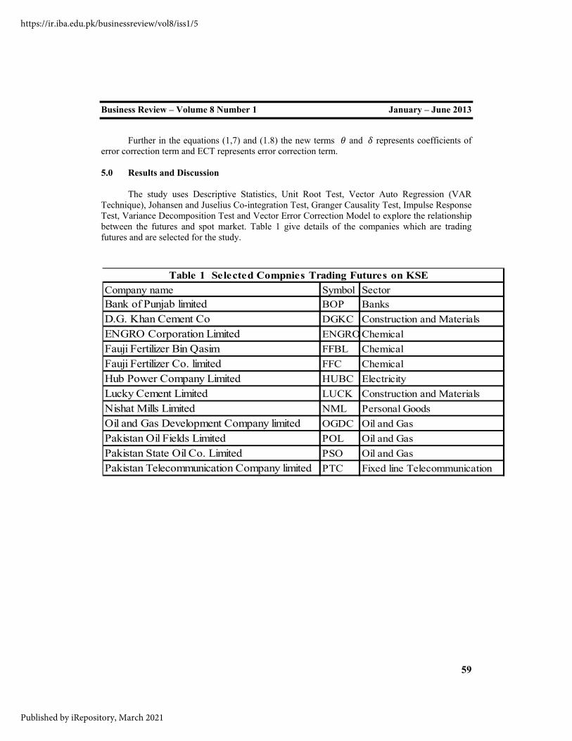
The study uses Descriptive Statistics, Unit Root Test, Vector Auto Regression (VAR Technique), Johansen and Juselius Co-integration Test, Granger Causality Test, Impulse Response Test, Variance Decomposition Test and Vector Error Correction Model to explore the relationship between the futures and spot market. Table 1 give details of the companies which are trading futures and are selected for the study.

Table 1 Selected Compnies Trading Futures on KSECompany name Symbol SectorBank of Punjab limited BOP BanksD.G. Khan Cement Co DGKC Construction and MaterialsENGRO Corporation Limited ENGRO ChemicalFauji Fertilizer Bin Qasim FFBL ChemicalFauji Fertilizer Co. limited FFC ChemicalHub Power Company Limited HUBC ElectricityLucky Cement Limited LUCK Construction and MaterialsNishat Mills Limited NML Personal GoodsOil and Gas Development Company limited OGDC Oil and GasPakistan Oil Fields Limited POL Oil and GasPakistan State Oil Co. Limited PSO Oil and GasPakistan Telecommunication Company limited PTC Fixed line Telecommunication




60

Note: FR denote (Futures Returns) and SR denotes (Spot Returns)

Descriptive statistics is applied on both the spot and futures returns of twelve companies for the period 2005 to 2010. The results in the table 2 reveal that OGDC spot producing the highest average monthly returns of 1.19% at 12.29% risk level. The OGDC futures average monthly returns is 1.13% and risk level of 12.64% which shows the futures are more risky and less productive than its spot returns. ENGRO’s spot average monthly returns hold the second position in the list with 0.89% and risk surface of 12.30%. The futures returns of ENGRO is 0.77% with risk level of 12.03% which shows the single stock futures of ENGRO is less productive than its underlying spot returns with almost the same level of risk. LUCK hold the third position with spot providing average monthly returns of 0.87% comparative to future return 0.86% . The risk level of spot is 15% and futures 20% showing that the futures trading on the stocks of LUCK is more risky than its underlying stock. The average monthly returns for spot and futures of four companies FFBL, HUBC, POL and PSO remain lower but positive with lower values of risk comparative to

Table 2 Results of Descriptive StatisticsCompanies Mean Median Maximum Minimum S.D Skewness Kurtosis Jarque Bera Prob Observation

BOP FR -0.0264 0.0000 0.4564 -0.8682 0.1822 -1.4696 8.8278 127.8040 0.0000 72

BOP SR -0.0265 0.0000 0.4562 -0.8739 0.1934 -1.2481 7.3131 74.5002 0.0000 72

DGKC FR -0.0083 -0.0036 0.5028 -0.6054 0.1676 -0.5505 5.1891 18.0136 0.0001 72

DGKC SR -0.0083 0.0000 0.5108 -0.6134 0.1702 -0.5881 5.1595 18.1411 0.0001 72

ENGRO FR

0.0077 0.0089 0.2888 -0.6169 0.1203 -1.8756 12.0217 286.3854 0.0000 72

ENGRO SR

0.0089 0.0092 0.2885 -0.6263 0.1230 -1.8255 11.6664 265.3113 0.0000 72

FFBL FR 0.0022 0.0131 0.1892 -0.3533 0.1043 -0.9477 4.1711 14.8918 0.0006 72

FFBL SR 0.0022 0.0111 0.1973 -0.3577 0.1024 -0.9627 4.4845 17.7316 0.0001 72

FFC FR -0.0015 0.0074 0.1728 -0.2304 0.0778 -0.7751 3.7856 9.0607 0.0108 72

FFC SR -0.0014 0.0026 0.1723 -0.2001 0.0723 -0.5627 3.5573 4.7311 0.0939 72

HUBC FR 0.0028 0.0041 0.2478 -0.2480 0.0859 -0.3779 4.3318 7.0353 0.0297 72

HUBC SR 0.0027 0.0030 0.2471 -0.2920 0.0909 -0.5260 4.5356 10.3941 0.0055 72

LUCK FR 0.0086 0.0060 0.9679 -0.6896 0.2061 0.4444 10.3181 163.0350 0.0000 72

LUCK SR 0.0087 0.0226 0.3008 -0.6138 0.1500 -1.0616 5.9840 40.2355 0.0000 72

NML FR -0.0027 0.0172 0.4058 -0.7265 0.1751 -1.1933 6.1104 46.1132 0.0000 72

NML SR -0.0039 0.0138 1.0295 -0.8662 0.2332 0.0203 10.0740 150.1292 0.0000 72

OGDC FR 0.0113 0.0197 0.3812 -0.6360 0.1264 -1.5919 11.7847 261.9235 0.0000 72

OGDC SR 0.0119 0.0137 0.3724 -0.6360 0.1229 -1.6711 12.9821 332.4352 0.0000 72

POL FR 0.0025 0.0140 0.3028 -0.8554 0.1548 -2.3969 14.9447 496.9707 0.0000 72

POL SR 0.0025 0.0170 0.3498 -0.8654 0.1659 -2.5267 14.2937 459.2562 0.0000 72

PSO FR 0.0003 0.0099 0.3268 -0.6601 0.1310 -1.6732 10.9242 221.9750 0.0000 72

PSO SR 0.0004 0.0083 0.3264 -0.6609 0.1284 -1.7135 11.8584 270.6432 0.0000 72

PTC FR -0.0119 0.0000 0.3265 -0.6166 0.1232 -1.4233 10.2439 181.7316 0.0000 72

PTC SR -0.0129 0.0000 0.3189 -0.6233 0.1198 -1.4416 11.4251 237.8870 0.0000 72




61

top three companies. Five companies namely BOP, DKCG, FFC, NML and PTC provide negative average monthly returns of both spot and futures with varying risk surface.

The statistics in the table 2 shows that the returns for all the companies are negatively skewed (except futures returns of LUCK and spot returns of NML which is positively skewed) which mean that the distribution has a long left tail with a higher probability of negative returns. When the Kurtosis is 3, the returns are Mesokurtic, when Kurtosis is >3 called Leptokrurtic and lastly when Kurtosis is <3 called Platykurtic. The Kurtosis of the future and spot returns for all the returns are greater than 3 showing that the distribution is peaked (Leptokurtic). It reflects that compared to normal distribution, the distribution of returns have a fat tails and consequently the Jorque-Bera test rejects the null hypothesis of normal distribution for all the companies. 1.1 Line graphs of spot and futures returns




62

5.2 Results of adf and phillip peron test

The statistics provided by the ADF and PP test reported in the table 3 rejects the null hypothesis of unit root. The statistics of both the tests complement each other revealing that the spot and futures monthly data series remains non-stationery at level, but become stationery at difference of 1. The t values of futures and spot prices of all the companies are smaller than the critical values (-3.527045, -2.903566 and -2.589227 at 1%, 5% and 10% significant level, respectively) show the rejection of null hypothesis of unit root at 1%, 5% and 10% significant level. The spot and futures series are integrated of I(1).

5.3 Vector auto regression (VAR technique)

The estimation of Johansen and Juselius Co-integration technique required appropriate lag selection. To find out the number of lags, Akaike Information Criterion and Shwarz Bayesian Criterion are the most commonly used methods in financial econometrics. The Values of AIC and SC were found minimum at lag 1 for the eleven companies namely BOP, DGKC, ENGRO, FFBL, HUBC, LUCK, NML, OGDC, POL, PSO and PTC. For FFC lag 3 have been selected for which the values of AIC and SC were at minimum. The statistics are provided in the table 4.

Table 3 Result of Unit root TestCompanies ADF Test ADF Test Phillip-Perron Test Phillip-Perron Test

at Level at 1st Difference at Level at 1st DifferenceBOP (Future Prices) -0.206 -8.0003 -0.2447 -8.0003

BOP (Spot Prices) -0.2836 -8.1185 -0.3115 -8.1185

DGKC(Future Prices) -1.3018 -6.665 -0.9294 -6.6427

DGKC(Spot Prices) -1.3018 -6.6181 -1.0878 -6.5745

ENGRO(Future Prices) -2.1127 -9.5114 -2.0449 -9.4983

ENGRO(Spot Prices) -2.1306 -9.5148 -2.1457 -9.5011

FFBL(Future Prices) -1.5972 -8.3235 -1.7941 -8.3568

FFBL(Spot Prices) -1.5552 -7.8266 -1.8554 -7.861

FFC(Future Prices) -2.7614 -7.6324 -2.0364 -9.1328

FFC(Spot Prices) -2.5344 -7.5982 -2.4489 -8.5016

HUBC(Future Prices) -1.736 -7.6778 -1.736 -7.6635

HUBC(Spot Prices) -1.8938 -8.0457 -1.9802 -8.0401

LUCK(Future Prices) -2.5842 -9.2222 -2.5842 -9.2883

LUCK(Spot Prices) -2.349 -6.4749 -2.2687 -6.4692

NML(Future Prices) -1.647 -9.2132 -1.6728 -9.1643

NML(Spot Prices) -2.1058 -10.827 -2.1058 -10.8103

OGDC(Future Prices) -2.0961 -7.171 -2.1717 -8.3509

OGDC(Spot Prices) -2.0843 -7.2465 -2.135 -8.0775

POL(Future Prices) -1.8793 -7.8628 -2.0181 -8.0393

POL(Spot Prices) -1.9725 -8.3984 -2.0114 -8.5349

PSO(Future Prices) -2.0056 -7.2614 -2.1402 -7.2744

PSO(Spot Prices) -2.4939 -7.1494 -2.1091 -7.1751

PTC(Future Prices) -0.9107 -8.225 -0.8599 -8.2507

PTC(Spot Prices) -0.8758 -8.1487 -0.8702 -8.159




63

5.4 Results of Johansen’s co-integration test

For the next step, the study applied Johansen and Juselius bivariate co-integration technique. Table 5 provides results for bivariate co-integration with maximum Eigen value statistics and table 6 provide results of bivariate co-integration with trace statistics for the spot and futures prices of mentioned twelve companies respectively.

Table 4 Statistics for selecting lag lenghtCompanies LAG 1 LAG 3 LAG4 LAG 5 LAG 6

AIC SBC AIC SBC AIC SBC AIC SBC AIC SBC AIC SBCBOP -2.9080 -2.7089 -2.8138 -2.4821 -2.7172 -2.2527 -2.6553 -2.0581 -2.6020 -1.8722 -2.6868 -1.8242

DKCG -5.2957 -5.0966 -5.2877 -4.9559 -5.2210 -4.7565 -5.1233 -4.5261 -5.0660 -4.3361 -5.1268 -4.2642

ENGRO -6.5882 -6.3892 -6.5150 -6.1832 -6.4431 -5.9786 -6.3697 -5.7725 -6.3941 -5.6642 -6.4143 -5.5517

FFBL -5.7087 -5.5096 -5.6484 -5.3166 -5.6058 -5.1413 -5.6360 -5.0388 -5.6524 -4.9225 -5.5687 -4.7061FFC -6.9318 -6.7327 -6.8789 -6.5471 -7.6641 -7.1996 -7.6338 -7.0366 -7.5411 -6.8112 -7.7789 -6.9163

HUBC -6.8585 -6.6595 -6.7577 -6.4259 -6.6754 -6.2109 -6.6233 -6.0261 -6.5856 -5.8557 -6.6361 -5.7735

LUCK -2.5753 -2.3762 -2.5802 -2.2485 -2.4714 -2.0069 -2.4012 -1.8041 -2.3232 -1.5933 -2.2114 -1.3488NML -1.8351 -1.6361 -1.7178 -1.3860 -1.6351 -1.1706 -1.5312 -0.9341 -1.4641 -0.7342 -1.3617 -0.4991

OGDC -5.6811 -5.4821 -5.6110 -5.2793 -5.5396 -5.0752 -5.4853 -4.8882 -5.4201 -4.6902 -5.3737 -4.5111

POL -4.1316 -3.9326 -4.0370 -3.7052 -3.9590 -3.4945 -3.9008 -3.3036 -3.8467 -3.1168 -3.7772 -2.9146PSO -7.2471 -7.0480 -7.2580 -6.9262 -7.3385 -6.8741 -7.2249 -6.6277 -7.2499 -6.5200 -7.1695 -6.3069

PTC -6.7169 -6.5178 -6.6118 -6.2800 -6.5120 -6.0476 -6.4614 -5.8642 -6.3573 -5.6274 -6.2737 -5.4111

LAG 2




64

The maximum eigenvalue statistics in table 5 reports one co-integration equation between the spot and futures prices of BOP, DGKC, FFBL, FFC, NML and PTC while two co-integration equation has been found between the spot and futures prices of ENGRO, HUBC, LUCK, OGDC, POL and PSO at 5% critical value.

Table 5 Results of Eigenvalue StatisticsCompanies Hypothesis Eigenvalue Max-Eigen Critical Value at 0.05 level RemarksBOP None * 0.2632 21.3814 14.2646 Existence of 1

At most 1 0.2632 21.3814 3.8415 Cointegration equationDGKC None * 0.2632 21.3814 ‐6.5817 Existence of 1

At most 1 0.2632 21.3814 ‐17.0048 Cointegration equationENGRO None * 0.2632 21.3814 ‐27.4279 Existence of 2

At most 1 * 0.2632 21.3814 ‐37.8511 Co‐integration equationsFFBL None * 0.2632 21.3814 ‐48.2742 Existence of 1

At most 1 0.2632 21.3814 ‐58.6973 Cointegration equationFFC None * 0.2632 21.3814 ‐69.1205 Existence of 1

At most 1 0.2632 21.3814 ‐79.5436 Cointegration equationHUBC None * 0.2632 21.3814 ‐89.9667 Existence of 2

At most 1 * 0.2632 21.3814 ‐100.3899 Co‐integration equationsLUCK None * 0.2632 21.3814 ‐110.8130 Existence of 2

At most 1 * 0.2632 21.3814 ‐121.2361 Co‐integration equationsNML None * 0.2632 21.3814 ‐131.6593 Existence of 1

At most 1 0.2632 21.3814 ‐142.0824 Cointegration equationOGDC None * 0.2632 21.3814 ‐152.5055 Existence of 2

At most 1 * 0.2632 21.3814 ‐162.9287 Co‐integration equationsPOL None * 0.2632 21.3814 ‐173.3518 Existence of 2

At most 1 * 0.2632 21.3814 ‐183.7749 Co‐integration equationsPSO None * 0.2632 21.3814 ‐194.1981 Existence of 2

At most 1 * 0.2632 21.3814 ‐204.6212 Co‐integration equationsPTC None * 0.2632 21.3814 ‐215.0443 Existence of 1

At most 1 0.2632 21.3814 ‐225.4675 Cointegration equation




65

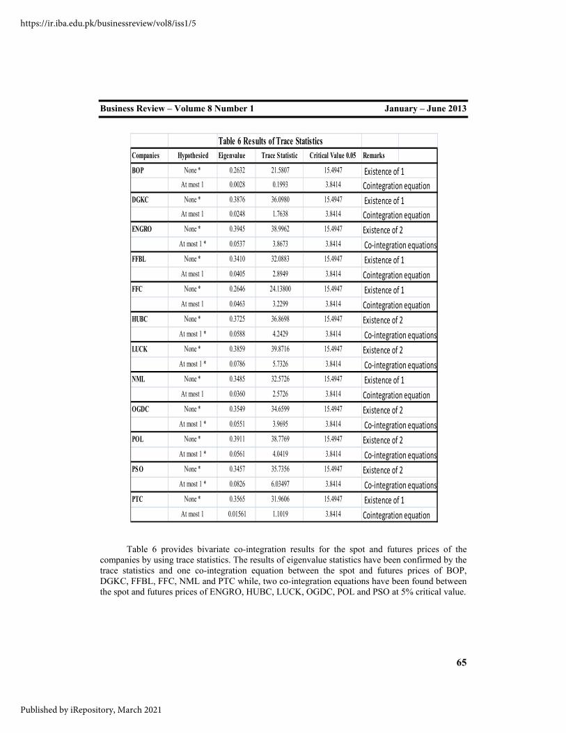
Table 6 provides bivariate co-integration results for the spot and futures prices of the companies by using trace statistics. The results of eigenvalue statistics have been confirmed by the trace statistics and one co-integration equation between the spot and futures prices of BOP, DGKC, FFBL, FFC, NML and PTC while, two co-integration equations have been found between the spot and futures prices of ENGRO, HUBC, LUCK, OGDC, POL and PSO at 5% critical value.

Table 6 Results of Trace StatisticsCompanies Hypothesied Eigenvalue Trace Statistic Critical Value 0.05 Remarks

BOP None * 0.2632 21.5807 15.4947 Existence of 1At most 1 0.0028 0.1993 3.8414 Cointegration equation

DGKC None * 0.3876 36.0980 15.4947 Existence of 1At most 1 0.0248 1.7638 3.8414 Cointegration equation

ENGRO None * 0.3945 38.9962 15.4947 Existence of 2At most 1 * 0.0537 3.8673 3.8414 Co‐integration equations

FFBL None * 0.3410 32.0883 15.4947 Existence of 1At most 1 0.0405 2.8949 3.8414 Cointegration equation

FFC None * 0.2646 24.13800 15.4947 Existence of 1At most 1 0.0463 3.2299 3.8414 Cointegration equation

HUBC None * 0.3725 36.8698 15.4947 Existence of 2At most 1 * 0.0588 4.2429 3.8414 Co‐integration equations

LUCK None * 0.3859 39.8716 15.4947 Existence of 2At most 1 * 0.0786 5.7326 3.8414 Co‐integration equations

NML None * 0.3485 32.5726 15.4947 Existence of 1At most 1 0.0360 2.5726 3.8414 Cointegration equation

OGDC None * 0.3549 34.6599 15.4947 Existence of 2At most 1 * 0.0551 3.9695 3.8414 Co‐integration equations

POL None * 0.3911 38.7769 15.4947 Existence of 2At most 1 * 0.0561 4.0419 3.8414 Co‐integration equations

PSO None * 0.3457 35.7356 15.4947 Existence of 2At most 1 * 0.0826 6.03497 3.8414 Co‐integration equations

PTC None * 0.3565 31.9606 15.4947 Existence of 1At most 1 0.01561 1.1019 3.8414 Cointegration equation




66

The above results suggest the existence of long run relationship between the spot and futures prices of these companies. 5.5 Results of Granger Causality

Granger Causality test shows that the spot returns of FFBL granger causes FFBL’s futures returns (P-value of 0.0133), Futures returns of HUBC granger causes HUBC’s spot returns (P-value of 0.0281), spot returns of LUCK granger causes futures returns of LUCK (P-value 0.0010) and futures returns of POL granger causes POL’s spot returns (P-value of 0.0052). The Granger Causality test for the remaining eight companies (BOP, DGKC, ENGRO, FFC, NML, OGDC, PSO, and PTC) does not predict any causal relationship between their spot and futures returns. The futures can help to forecast the spot in case of HUBC and POL and play its important role of price discovery. The spot can forecast the futures in case of FFBL and LUCK and the result is line with Khan (2006) paper for the Futures trading and Price Discovery in Pakistan. The Ganger Causality has a mix results and both the spot and futures play important role in forecasting their respective futures and spot prices. The results of Granger Causality Test are provided in the table 7.

Table 7 Result of Granger Causality TestCompanies Null hypothesis F statistics Probability BOP BSR does not Granger Cause BFR 0.1244 0.7254

BFR does not Granger Cause BSR 0.9153 0.3421

DGKC DGSR does not Granger Cause DGFR 0.4882 0.4871 DGFR does not Granger Cause DGSR 0.2456 0.6217

ENGRO ENGR_SR does not Granger Cause ENGR_FR 0.0522 0.8199 ENGR_FR does not Granger Cause ENGR_SR 0.0785 0.7801

FFBL FFBL_SR does not Granger Cause FFBL_FR 6.4650 0.0133 FFBL_FR does not Granger Cause FFBL_SR 0.3498 0.5562

FFC FFC_SR does not Granger Cause FFC_FR 2.1138 0.1075 FFC_FR does not Granger Cause FFC_SR 2.3010 0.0859

HUBC HUBC_SR does not Granger Cause HUBC_FR 0.6114 0.4370 HUBC_FR does not Granger Cause HUBC_SR 5.0377 0.0281

LUCK LUCK_SR does not Granger Cause LUCK_FR 11.8867 0.0010 LUCK_FR does not Granger Cause LUCK_SR 0.0015 0.9686

NML NML_SR does not Granger Cause NML_FR 0.7142 0.4010 NML_FR does not Granger Cause NML_SR 2.0271 0.1591

OGDC OGDC_SR does not Granger Cause OGDC_FR 2.3520 0.1298 OGDC_FR does not Granger Cause OGDC_SR 0.0001 0.9892

POL POL_SR does not Granger Cause POL_FR 0.9315 0.3379 POL_FR does not Granger Cause POL_SR 8.3461 0.0052

PSO PSO_SR does not Granger Cause PSO_FR 0.2529 0.6166 PSO_FR does not Granger Cause PSO_SR 0.0575 0.8112

PTC PTC_SR does not Granger Cause PTC_FR 0.0010 0.9747 PTC_FR does not Granger Cause PTC_SR 0.7951 0.3757




67

5.6 Results of impulse response




68

The above Figure provides results of impulse response test for the twelve companies. The impulse response analysis represents that the shocks in the futures markets of all the selected companies are explained by their own innovations and their respective spot markets have less influence on them.

5.7 Results of variance decomposition test

Table 8 provides results for Variance Decomposition test. The results shows that any variation in futures returns is explained more by its own lag returns (100%) than by the lag retunes of spot. From the results of variance decomposition test, we can conclude that futures market of all the companies is an exogenous market as majority of its stocks are explained by its own innovations.

5.8 Results of Vector Error Correction Model

Lein (1996) argued that when two series are found to be co-integrated, a VAR technique along with error correction term should be estimated. The error correction model based on ARDL

Table 8 Result of Variance Decomposition TestPeriod 1 2 3 4 5 6 7 8 9 10S.E 0.1854 0.1859 0.1859 0.1859 0.1859 0.1859 0.1859 0.1859 0.1859 0.1859

FRBOP 100.0000 99.8346 99.8261 99.8252 99.8251 99.8251 99.8251 99.8251 99.8251 99.8251SRBOP 0.0000 0.1654 0.1739 0.1748 0.1749 0.1749 0.1749 0.1749 0.1749 0.1749S.E 0.1664 0.1709 0.1711 0.1712 0.1712 0.1712 0.1712 0.1712 0.1712 0.1712

FRBOP 100.0000 99.4940 99.4567 99.4378 99.4341 99.4330 99.4328 99.4327 99.4327 99.4327SRBOP 0.0000 0.5060 0.5433 0.5622 0.5659 0.5670 0.5672 0.5673 0.5673 0.5673S.E 0.1211 0.1223 0.1223 0.1223 0.1223 0.1223 0.1223 0.1223 0.1223 0.1223

FRBOP 100.0000 99.9470 99.9303 99.9268 99.9261 99.9260 99.9260 99.9260 99.9260 99.9260SRBOP 0.0000 0.0530 0.0697 0.0732 0.0739 0.0740 0.0740 0.0740 0.0740 0.0740S.E 0.1015 0.1050 0.1057 0.1059 0.1060 0.1060 0.1060 0.1060 0.1060 0.1060

FRBOP 100.0000 93.5587 92.3168 91.9509 91.8477 91.8182 91.8098 91.8074 91.8067 91.8065SRBOP 0.0000 6.4413 7.6832 8.0491 8.1523 8.1818 8.1902 8.1926 8.1933 8.1935S.E 0.0755 0.0757 0.0778 0.0795 0.0799 0.0803 0.0812 0.0814 0.0815 0.0819

FRBOP 100.0000 99.9144 99.5282 95.4079 94.4645 93.6017 92.0257 91.9774 91.5846 91.1090SRBOP 0.0000 0.0856 0.4718 4.5921 5.5355 6.3983 7.9743 8.0226 8.4155 8.8910S.E 0.0869 0.0875 0.0876 0.0876 0.0876 0.0876 0.0876 0.0876 0.0876 0.0876

FRBOP 100.0000 99.3139 99.2182 99.1994 99.1959 99.1953 99.1951 99.1951 99.1951 99.1951SRBOP 0.0000 0.6861 0.7818 0.8006 0.8041 0.8047 0.8049 0.8049 0.8049 0.8049S.E 0.1932 0.2073 0.2098 0.2104 0.2106 0.2106 0.2106 0.2106 0.2106 0.2106

FRBOP 100.0000 87.1794 86.7057 86.3666 86.3140 86.2978 86.2943 86.2934 86.2932 86.2931SRBOP 0.0000 12.8206 13.2943 13.6334 13.6860 13.7022 13.7057 13.7066 13.7068 13.7069S.E 0.1756 0.1768 0.1771 0.1771 0.1771 0.1771 0.1771 0.1771 0.1771 0.1771

FRBOP 100.0000 99.2136 98.9602 98.8965 98.8811 98.8774 98.8765 98.8762 98.8762 98.8762SRBOP 0.0000 0.7864 1.0398 1.1035 1.1189 1.1227 1.1235 1.1238 1.1238 1.1238S.E 0.1261 0.1284 0.1287 0.1288 0.1288 0.1288 0.1288 0.1288 0.1288 0.1288

FRBOP 100.0000 97.4195 97.0688 96.9731 96.9511 96.9458 96.9445 96.9442 96.9441 96.9441SRBOP 0.0000 2.5805 2.9312 3.0269 3.0489 3.0542 3.0555 3.0558 3.0559 3.0559S.E 0.1567 0.1579 0.1581 0.1581 0.1581 0.1581 0.1581 0.1581 0.1581 0.1581

FRBOP 100.0000 99.0183 98.8496 98.8153 98.8084 98.8070 98.8067 98.8066 98.8066 98.8066SRBOP 0.0000 0.9817 1.1504 1.1847 1.1916 1.1930 1.1933 1.1934 1.1934 1.1934S.E 0.1310 0.1333 0.1334 0.1334 0.1334 0.1334 0.1334 0.1334 0.1334 0.1334

FRBOP 100.0000 99.7422 99.7169 99.7066 99.7043 99.7036 99.7035 99.7034 99.7034 99.7034SRBOP 0.0000 0.2578 0.2831 0.2934 0.2957 0.2964 0.2965 0.2966 0.2966 0.2966S.E 0.1186 0.1189 0.1189 0.1189 0.1189 0.1189 0.1189 0.1189 0.1189 0.1189

FRBOP 100.0000 99.9988 99.9987 99.9987 99.9987 99.9987 99.9987 99.9987 99.9987 99.9987SRBOP 0.0000 0.0012 0.0013 0.0013 0.0013 0.0013 0.0013 0.0013 0.0013 0.0013

HUBC

LUCK

NML

OGDC

POL

PSO

PTC

BOP

DGKC

ENGRO

FFBL

FFC




69

approach has been applied to test for the short term relationship between the spot and futures returns of the mentioned companies. The coefficient ECM (-1) shows how much of the short run disequilibrium will be eliminated in the long run. The error correction variable ECM for all the companies has been reported negative and also statistically significant. Futures returns have been considered as dependent variable while spot return as independent variable.

From the result of Vector Error Correction Model in table 9, it is clear that 100% of the previous month’s disequilibrium in the futures returns will be corrected in the current month for the BOP, while this figure for DGKC, ENGRO, FFBL, FFC, HUBC, LUCK, NML, OGDC, POL, PSO and PTC is quite high with value of 150%, 143%, 151%, 252%, 143%, 149%, 133%, 148%, 146%, 151% and 142%. We can conclude that the adjustment process in case of disequilibrium is quite fast for all the companies. 6.0 Conclusion

The study was conducted to analyze the relationship of single stock futures with the underlying stock on which future is traded. Twelve companies from different sectors which are

Table 9 Results of Variance Decomposition TestCompany Regressor Coefficient Standard Error T-Ratio Probability

BOP SRBOP 0.8563 0.0473 18.0929 [.000]

ecm(-1) -1.0000 0.0000 *NONE* [.000]

DGKC SRDGKC 0.9703 0.0202 48.0280 [.000]

ecm(-1) -1.5044 0.1047 -14.3736 [.000]

ENGRO SRENGRO 0.97089 0.020987 46.2611 [.000]

ecm(-1) -1.4302 0.10268 -13.9284 [.000]

FFBL SRFFBL 0.8395 0.0600 13.9916 [.000]

ecm(-1) -1.5120 0.0993 -15.2311 [.000]

SR1FFC 0.71645 0.085866 8.3438 [.000]

FFC SRFFC 1.0108 0.050306 20.0938 [.000]

SR1FFC -0.76821 0.0877 -8.7595 [.000]

ecm(-1) -2.5244 0.14622 -17.2648 [.000]

HUBC SRHUBC 0.9264 0.0353 26.2105 [.000]

ecm(-1) -1.4319 0.1135 -12.6127 [.000]

LUCK SRLUCK 0.1045 0.0353 9.3162 [.000]

ecm(-1) -1.4931 0.1054 -14.1607 [.000]

NML SRNML 0.56497 0.064821 8.7158 [.000]

ecm(-1) -1.3368 0.11115 -12.0272 [.000]

OGDC SROGDC 0.9765 0.0325 30.0375 [.000]

ecm(-1) -1.4883 0.1052 -14.1539 [.000]

POL SRPOL 0.9120 0.0433 21.0436 [.000]

ecm(-1) -1.4681 0.1151 -12.7514 [.000]

PSO SRPSO 1.0163 0.0135 75.1676 [.000]

ecm(-1) -1.5174 0.1030 -14.7385 [.000]

PTC SRPTC 1.0177 0.0230 44.2509 [.000]

ecm(-1) -1.4227 0.1101 -12.9275 [.000]




70

trading single stock futures on their stocks were considered for a period of six years from 1 January, 2005 to 31 December, 2010 for this study. The result of unit root indicates that the series of futures and spot are non-stationery at level, but become stationery at first difference. To check for any long run relationship, Johansen’s co-integration technique was used. The maximum eigenvalue statistics and trace statistics reports one co-integration equation between the spot and futures prices of BOP, DGKC, FFBL, FFC, NML and PTC while two co-integration equations has been found between the spot and futures prices of ENGRO, HUBC, LUCK, OGDC, POL and PSO at 5% critical value. The results confirm the existence of long run relationship between the futures and spot prices of all the companies. To explore the causal effect, Granger Causality test has been applied. The result of Granger Causality test predicts that the spot prices of FFBL and LUCK assist in forecasting their respective futures prices which is in line with the results reported by Khan (2006). The futures prices of HUBC and POL forecast their respective spot prices. Thus the lead lags relationship between spot and futures are mix. The Futures for HUBC and POL can predict the expected spot prices in the future and play its important role of price discovery. No causal relationship has been found between the spot and futures returns of the remaining eight companies.

Vector error correction model based on ARDL approach captures the short-run dynamics of relationship between the spot and futures returns. The results of VECM establish that the error correction variable ECM (-1) for all the companies has been found negative and also statically significant. The results of VECM reported that 100% of the previous month’s disequilibrium in the futures returns will be corrected in the current month for the BOP, while this figure for DGKC, ENGRO, FFBL, FFC, HUBC, LUCK, NML, OGDC, POL, PSO and PTC is quite high with value of 150%, 143%, 151%, 252%, 143%, 149%, 133%, 148%, 146%, 151% and 142%. The results of VECM shows that in case of disequilibrium the adjustment process is quite fast for all the companies.

To investigate the dynamic response between spot market and futures market, impulse response and variance decomposition tests are applied. The impulse response analysis represents most of the shocks in the futures markets of all the selected companies are explained by their own innovations and their respective spot markets have less influence on them. From the results of variance decomposition test we can conclude that futures market is an exogenous market as majority of its stocks are explained by its own innovations.

The empirical results of the study suggest the existence of long run relationship between the spot and futures market. The existence of long run relationship can provide benefits to investors by using futures and spot market in their hedging strategy. Ederington (1979) presumes that strong co movement between two markets is necessary for efficient hedging. The result of impulse response shows that the futures of all companies have a small response to the shock in the underlying spot market and the impulse response gradually dies out predicting co-integration between the spot and futures market which confirm Johansen’s co-integration results.

The probability of negative returns is high than positive returns in both the spot and futures returns of the companies which mean downside risk is more compare to upside risk. The returns are more volatile between 2008 and 2009 which can be attributed to both financial crisis and political instability in the country.




71

6.1 Practical implication

The study provides important information for investors about the futures market in Pakistan. The existence of long run relationship and the role of futures market in price discovery show that investors can use the futures market for risk management and efficient hedging.

6.2 Futures research direction

Futures research can explore the sources of instabality in the spot and futures market and and further considering the volatlity effect in the spot and futues market. References A.Sims, C., 1972. Money,Income and Causality. The American Economic Review, 62(4), pp.540-52. Abdulah, M. et al., 2001. "The Temporal Price Relationship between the Stock Index Futures and the Underlying Stock Index: Evidence from Malaysia". Journal of Social Sciences and Humanities , pp.73-84. Ahmad, H., Shah, S.Z.A. & Shah, I.A., 2010. "Impact of Futures Trading on Spot Price Volatility:Evidence from Pakistan". International Research Journal of Finance and Economics, (59), pp.145-65. Alexakis, P., 2007. On the Effect of Index Futures Trading on Stock Market. International Research Journal of Finance and Economics, (11), pp.7-20. Alphonse, P., 2000. Efficient Price Discovery in Stock Index Cash and Futures Markets. Annals of Economics and Statistics, pp.177-88. Antoniou a, A. & Holmes, P., 1995. "Futures trading, information and spot price volatility: evidence for the FTSE-100 Stock Index Futures contract using GARCH". Journal of Banking & Finance, 19, pp.117-29. Antoniou b, A. & Garrett, I., 1993. "To What Extent did Stock Index Futures Contribute to the October 1987 Stock Market Crash?" The Economic Journal, 103, pp.1444-61. Antoniou c, A., Koutmos, G. & Pericli, A., 2005. "Index futures and positive feedback trading:evidence from major stock exchanges". Journal of Empirical Finance, 12, pp.219-38. Bae, S.C., Kwon, T.H. & Park, J.W., 2004. Futures trading, Spot market volatility, and market Efficiency: The case of the Korean Index Futures markets. The Journal of Futures Markets, 24, p.1195–1228. Becketti, S. & J.Roberts, D., 1990. "Will increased Regualtion of Stock indes Futures reduce Stock Market Volatility?" Economic review, pp.33-46.




72

Bessembinder, H. & Seguin, P.J., 1992. "Futures-Trading Activity and Stock Price Volatility". The Journal of Finance, 47, pp.2015-34. Bhar, R., 2001. "Return and Volatility Dynamics in the Spot and Futures Markets in Australia: An Intervention Analysis in a Bivariate EGARCH-X Framework". Journal of Futures Markets, 21, pp.833-50. Bohl, M.T., Salm, C.A. & wilfling, B., 2011. "Do individual index futures investors destabilize the Underlying spot market?" The Journal of Futures Markets, 31, pp.81-101. Bollerslev, T., 1986. "Generalized Autoregressive Conditional Heteroskedasticity". Journal of Econometrics, 31, pp.307-27. Bologna, P. & Cavallo, L., 2002. "Does the introduction of stock index futures effectively reduce stock market volatility? Is the 'futures effect' immediate? Evidence from the Italian stock exchange using GARCH". Applied Financial Economics, 12, pp.183-92. Bose, S., 2007. "Understanding the Volatility Characteristics and Transmission Effects in the Indian Stock Index and Index Future market". ICRA Bulletin, Money & Finance, pp.139-62. Brooks, C., Rew, A.G. & Ritson, S., 2001. "A trading strategy based on the lead–lag relationship between the spot index and futures contract for the FTSE 100". International Journal of Forecasting, pp.31-44. Chang, E.C., Cheng, J.W. & Pinegar, J.M., 1999. "Does futures trading increase stock market volatility? The case of the Nikkei stock index futures markets". Journal of Banking & Finance, 23, pp.727-53. Chatrath a, A. & Song, F., 1998. "Information and Volatility in Futures and Spot Markets: The Case of the Japanese Yen". The Journal of Futures Markets, 18, p.201–223. Chatrath b, A., Ramchander, S. & Song, F., 1998. Speculative Activity and Stock Market Volatility. Journal of Economics and Business 1998; 50:, 50, p.323–337. Chiang, M.-H. & Wang, C.-Y., 2002. "The impact of futures trading on spot index volatility: evidence for Taiwan index futures". Applied Economics Letters, 9, pp.381-85. Chuang, C.-C., 2003. "International Information Transmissions between Stock Index Futures and Spot Markets: The Case of Futures Contracts Related to Taiwan. Journal of Management Sciences, 19, pp.51-78. Covey, T. & Bessler, A.D., 1992. Testing for Granger's full causality. Review of Economics and Statistics , 74, pp.146-53.




73

Covrig, V. & Ding, K.D., 2004. The contribution of a Satellite market to price discovery: Evidence from the Singapore exchange. Journal of Futures Market, pp.981-1004. D.Garbade, K. & L.Silber, W., 1983. Price Movements and Price Discovery in Futures and Cash Markets. The Review of Economoics and Statistics, 65(2), pp.289-97. D.Mackenzie, M., J.Brailsford, T. & W.Faff, R., 2000. “New insight into the impact of the introduction of futures trading on stock price volatility”. Working paper series in finance. Darrat, A.F., Rahman, S. & Zhong, M., 2002. "On The role of Futures Trading in Spot market fluctuations: Perpetrator of Volatility or victim of regret?" The Journal of Financial Research, 3, p.431–444. Debasish, S.S., 2009. "Effect of futures trading on spot-price volatility: evidence for NSE Nifty using GARCH". The Journal of Risk Finance, 10, pp.67-77. Dennis, S.A. & Sim, A.B., 1999. "Share price volatility with the introduction of individual share futures on the Sydney Futures Exchange". International Review of Financial Analysis, 8, pp.153-63. Drimbetas, E., Sariannidis, N. & Porfiris, N., 2007. "The effect of derivatives trading on volatility of the underlying asset: evidence from the Greek stock market". Applied Financial Economics, 17, pp.139-48. Ederington, L.H., 1979. The Hedging Performance of the New Futures Markets. The Journal of Finance, 34(1), pp.157-70. Edwards, F.R., 1988. "Does Futures Trading Increase Stock Market Volatility?" Financial Analysts Journal, 44, pp.63-69. England, B.O., 1988. "The Equity market crash Bank of England Quarterly Bulletin". Engle, R.F. & Ng, V.K., 1993. "Measuring and testing the impact of news on volatility". Journal of Finance, 48, p.1749–1778. F.Engle, R. & Granger, C.W.J., 1987. Co-integration and Error Correction: Representation, Estimatin and Testing. Econometrica, 55(2), pp.251-76. Faff, R.W. & McKenzie, M.D., 2002. "The Impact of Stock Index Futures Trading on Daily Returns Seasonality: A Multicountry Study". Journal of Business, 75, pp.95-125. Filis, G., Floros, C. & Eeckels, B., 2011. "Option listing, returns and volatility: evidence from Greece". Applied Financial Economics, 21, pp.1423-35. Flemming, J., Ostdiek, B. & E.Whaley, R., 1996. Trading Cost and the Relative Rates of Price Discovery in Stock,Futures and Option Markets. Jounrnal of Futures Markets, 16(4).




74

Floros, C., 2009. Price Discovery in the South African Stock Index Futures Market. International Research Journal of Finance and Economics, pp.148-59. Gahlot, R. & Datta, S.K., 2011. "Impact of Future Trading on Efficiency and Volatility of the Indian Stock Market:A Case of CNX 100". Journal of Transnational Management, 16, pp.43-57. Galloway, T.M. & Miller, J.M., 1997. "Index Futures Trading and Stock Return Volatility: Evidence from the Introduction of MidCap 400 Index Futures". The Financial review, 32, pp.845-66. Granger, C.W.J., 1969. Investigating Causal Relation by Econometric Models and Cross-spectral Methods. Econometrica, 37(3), pp.424-38. Grossman a, S.J., 1988. "An Analysis of the Implications for Stock and Futures Price Volatility of Program Trading and Dynamic Hedging Strategies". The Journal of Business, 61, pp.275-98. Grossman b, S.J., 1988. "Program Trading and Market Volatility: A Report on Interday Relationships". Financial Analysts Journal, 44, pp.18-28. Harris, L., 1989. "S&P 500 Cash Stock Price Volatilities". The Journal of Finance, 44, pp.1155-75. Hernandez-Trillo, F., 1999. "Financial derivatives introduction and stock return volatility in an emerging market without clearinghouse: The Mexican experience". Journal of Empirical Finance, 6, p.153–176. Hicks, J.R., 1946. Value and Capital. Oxford: Clarendon. Ibrahim, A.J., Othman, K. & Bacha, O.I., 1999. "Issues In Stock Index Futures Introduction And Trading. Evidence From The Malaysian Index Futures Market". Capital Markets Review, 7, pp.1-46. Jegadeesh, N. & Subrahmanyam, A., 1993. "Liquidity Effects of the Introduction of the S&P 500 Index Futures Contract on the Underlying Stocks". The Journal of Business, 66, pp.171-87. Jiang, S.-j., Chang, M.C. & Chiang, I.-c., 2011. Price discovery in stock index: an ARDL-ECM approach in Taiwan case. QUALITY & QUANTITY. Kan, A.C.N., 1997. "The effect of index futures trading on volatility of HSI constituent stocks: A note". Pacific-Basin Finance Journal, 5, pp.105-14. Kasman, A. & Kasman, S., 2008. "The impact of futures trading on volatility of the underlying asset in the Turkish stock market". Physica A, 387, p.2837–2845. Katzenbach, 1987. "An Overview of Program Trading and Its Impact on Current Market Practices".




75

Keynes, J.M., 1923. Some aspects of commodity markets. Manchester: Guardian Commercial. Khan, S., 2006. "Role of the Futures Market on Volatility and Price Discovery of the Spot Market: Evidence from Pakistan’s Stock Market". The Lahore journal of Economics, 11, pp.107-21. Kumar, K.K., 2007. "Impact of Futures Introduction on Underlying Index Volatility: Evidence from India". Journal of Management Science, 1, pp.26-42. Kuo, H.W., Hsu, H. & Chiang, H.M., 2008. Foreign investment, regulation, volatility spillovers between the futures and spot markets: evidence from Taiwan. Applied Financial Economics, 18, pp.421-30. L.Hemler, M. & Longstaff, F.A., 1991. General Equilibrium Stock Index Futures Prices: Theory and Empirical Evidence. Journal of Finance and Quantitative Analysis, 26(3), pp.287-308. Lee, S.B. & Ohk, K.Y., 1992. "Stock index futures listing and structural change in time-varying volatility". The Journal of Futures Markets, 12, p.493–509. Lee, C.I. & Tong, H.C., 1998. "Stock futures: the effects of their trading on the underlying stocks in Australia". Journal of Multinational Financial Management, 8, pp.285-301. Lein, D.D., 1996. The effect of the Co-integration Relationship on Futures hedging: a note. Journal of Futures Markets , 16, pp.733-89. M.Illueca & J.A.Lafuente, 2003. "The Effect of Spot and Futures trading on Stock Index Market Volatility: A Nonparametric Approach". The Journal of Future Markets, 23, pp.841-58. Mckenzie, D.M., Brailsford, J.T. & Faff, R.W., 2000. New insight into the impact of the introduction of futures trading on stock price volatility. Working paper series in finance. Min, J.H., 2002. "Program Trading and Intraday Volatility in the Stock Index Futures Market and Spot Market: The Case of Korea". Journal of Asia-Pacific Business, 4, pp.53-68. Morris, C.S., 1989. Managing Stock Market Risk with stock Index Futures. Economic Review. Nelson, D.B., 1991. "Conditional heteroskedasticity in asset returns: a new approach". Econometrica, 59, pp.347-70. Pericli, A. & Koutmos, G., 1997. "Index Futures and Options and Stock market volatility". The Journal of Futures Markets, 17, p.957–974. Pizzi, M.A., Economopoulos, A.J. & O'Neill, H.M., 1998. An examination of the relationship between stock index cash and futures markets: A cointegration approach. Journal of Futures Markets, 18(3), pp.297-305.




76

Pok, W.C. & Poshakwale, S., 2004. "The impact of the introduction of futures contracts on the spot market volatility: the case of Kuala Lumpur Stock Exchange". Applied Financial Economics, 14, pp.143-54. Powers, M.J., 1970. "Does Futures Trading Reduce Price Fluctuations in the Cash Markets?" The American Economic Review, 60, pp.460-64. R.Stoll, H. & E.Whaley, R., 1988. "The Dynamics of Stock Index and Stock Index Futures returns". Journal of Financial and Quantitatve Analysis, 25, pp.441-68. Ryoo, H.-J. & Smith, G., 2004. "The impact of stock index futures on the Korean stock market". Applied Financial Economics, 14, pp.243-51. S.Morris, C., 1990. Coordinating circuit breakers in stock and futures markets. Economic Review. Samuelson, P.A., 1965. Proof that properly Anticipated Prices Fluctuate Randomly. Management Review, 6(2). Schwarz, T.V. & Laatsch, F.E., 1991. Dynamic Efficiency and Price Leadership in Stock Index Cash and Futures Markets. The Journal of Futures Markets, 11, pp.669-83. Spyrou, S.I., 2005. "Index Futures Trading and Spot Price Volatility:Evidence from an Emerging Market". Journal of Emerging Market Finance, 4, pp.151-67. Strong, R.A., 2005. Derivatives: an introduction. 2nd ed. Mason Ohio: Thomson South Western. Subrahmanyam, A., 1991. A theory of Trading in Stock index Futures. The Review of Financial Studies, 4(1), pp.17-51. Telser, L.G., 1981. Margins and futures contracts. Journal of Futures Markets, 1(2), pp.255-53. V.v.Chari, R.J. & Jones, L., 1990. Price Stability and Futures Trading in commodities. Journal of Economics, 105(2), pp.527-34. Yang, J., Balyeat, R.B. & J.Leatham, D., 2005. "Futures Trading Activity and Commodity Cash Price Volatility". Journal of Business Finance & Accounting, 32(1-2), pp.297-323. YanG, J., Bessler, D.A. & Leatham, D.J., 2001. "Asset Storability and Price Discovery in Commodity Futures Market". The Journal of Futures Markets, 21, No. 3, p.279–300. Yu, S.W., 2001. "Index futures trading and spot price volatility". Applied Economics Letters, 8, pp.183-86.



Date post:	23-Oct-2021
Category:	Documents
Upload:	others
View:	3 times
Download:	0 times

Relationship of single stock futures with the spot price ...

Documents