Relationships between water attenuation coefficientsderived from active and passive remote sensing:
a case study from two coastal environments
Martin A. Montes,1,* James Churnside,3 Zhongping Lee,1 Richard Gould,2
Robert Arnone,2 and Alan Weidemann2
1Geosystems Research Institute, Mississippi State University, Mississippi 39529, USA2Naval Research Laboratory, Stennis Space Center, NASA, Mississippi 39529, USA
3Earth System Research Laboratory, National Oceanic and Atmospheric Administration,Boulder, Colorado 80305, USA
The diffuse attenuation coefficient of downwellingirradiance (Kd) is a key optical property linked to thevariability of underwater light fields in aquatic en-vironments [1]. For this reason, Kd has often beenused by modelers to estimate the depth of the eupho-tic zone (i.e., the depth at which irradiance is 1% ofsurface value) [2]. Also, Kd has been commonly usedto calculate solar heat budgets [3], determine lightthresholds for prey–predator relationships [4],estimate coral reef mortality due to thermal stress[5], and indicate water quality status in coastalstudies [6].
The magnitude and vertical distribution of Kdare determined by the sunlight geometry and the
inherent optical properties of the water [7]. In simpleterms, Kd is directly related to the total (waterþparticulates) scattering (b) and absorption coefficient(a), and inversely related to the average cosine ofthe zenith angle of refracted solar photons (directbeam) just beneath the sea surface (μ0) (Table 1).Far from the sea surface, the Kd distribution ismainly driven by variations on the absorption co-efficient [8]. Attenuation of the lidar volume back-scattering with depth (α) is fully or partially linkedto Kd, depending on the lidar spot size at the seasurface (R ¼ Hθreceiver, where H is the lidar carrieraltitude above the sea surface and θreceiver is thereceiver’s field of view) and the beam attenuationcoefficient (c ¼ aþ b) [8]. Assuming a verticallyhomogeneous distribution of inherent optical proper-ties, when cR ≪ 1, the exponential decrease of lidarvolume backscattering (S) with depth is principallyexplained by single scattering and α → c [9]:
where ζ is the lidar range, Q is the pulse energy, Arcvis the area of the receiver, Tatm and Taw are the trans-mission of the atmosphere and the air/water inter-face, respectively, βðπÞ is the volume backscatteringevaluated at a scattering angle of 180°, v is the speedof light in vacuum, and m is the refractive index ofseawater. Conversely, when cR ≫ 1, multiple scatter-ing dominates the received signal, and Eq. (1) is nolonger a good approximation due to the effects of vo-lume scattering function shape (i.e., forward versusbackward directions) and variations associated withthe transmitter beam width. In this case, α → Kd,and the lidar volume backscattering can be modeledaccording to the following expression [9]:
where μ and σ2 are the mean and variance of theGamma probability density function of photons asa function of lidar range and time. The cR valuecorresponding to the transition between the “single-backscattering” and “multiple-forward- scattering”regimes is still in debate due to differences between
lidar models [8,9]. One way to study the cR thresholdfor a specific lidar system is to compare simultaneousα values with field measurements of inherent opticalproperties [10]. This method works when lidar andoptical passive observations are concurrent, andhave associated a minimum measurement error dueto instrument self-shading effects.
Unlike Kd, optical properties influenced by for-ward scattering of photons (e.g., c, volume scatteringfunction, and backscattering efficiency [i.e., ~bb ¼bb=b, where bb is the total (waterþ particulates)backscattering coefficient] are difficult or impossibleto study based on remote sensing reflectance (Rrs)signatures [11]. For this reason, most of studies re-porting b, ~bb, and c distributions in surface oceanicand coastal waters rely on more accurate methodsbased on in-water determinations [12,13]. Althoughrelatively accurate (∼15%) [14,15], retrievals of Kd,a, and bb based on spaceborne or airborne passivesensors are not vertically resolved, thus they re-present integrated values within the first opticaldepth. This depth restriction is alleviated when ac-tive optical systems, such as lidars, are used instead.However, Kd values computed from lidar volumebackscattering profiles are commonly quantifiedwith fewer wavelengths with respect to those Kd va-lues derived from Rrs measurements obtained withpassive optical systems. Another difference to em-phasize is that α is not necessarily equivalent toKd due to the variable contribution of forward scat-tering at the lidar receiver. Therefore, for a specificlight wavelength, α provides additional information
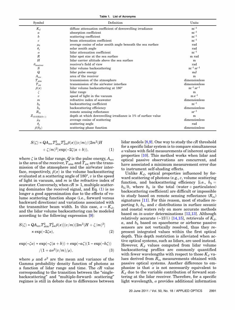
Table 1. List of Acronyms
Symbol Definition Units
Kd diffuse attenuation coefficient of downwelling irradiance m−1
a absorption coefficient m−1
b scattering coefficient m−1
c beam attenuation coefficient m−1
μ0 average cosine of solar zenith angle beneath the sea surface radθz solar zenith angle radα lidar attenuation coefficient m−1
R lidar spot size at the sea surface m radH lidar carrier altitude above the sea surface m
θreceiver receiver’s field of view radS lidar volume backscattering m−1 sr−1
Q lidar pulse energy mJArcv area of the receiver mTatm transmission of the atmosphere dimensionlessTaw transmission of the air/water interface dimensionlessβðπÞ lidar volume backscattering at 180° m−1 sr−1
ζ lidar range mv speed of light in the vacuum ms−1
m refractive index of seawater dimensionlessbb backscattering coefficient m−1
relative to Kd that can be exploited in combinationwith passive measurements to extract c, b,and ~bb.
The aim of this study is to investigate how α valuesderived from an airborne backscattering-based lidar(i.e., the National Oceanic and Atmospheric Admin-istration’s Fish Lidar Oceanic Experimental system)relate to Kd values computed from spaceborne Rrsmeasurements having a moderate spatial resolution(∼1:1km) (Objective 1), and to apply these measure-ments to estimate b, ~bb, and c within the first opticaldepth of two coastal areas (Oregon/Washingtonand the Afgonak/Kodiak Shelves) characterized bywaters having different optical composition (Objec-tive 2). Because of the field of view of our lidar recei-ver and the relatively high turbidity of the watersunder investigation, we hypothesize a substantialcorrelation between satellite-derived Kd and lidar-based measurements of α.2. Experiments
A. Study Areas and Sampling Design
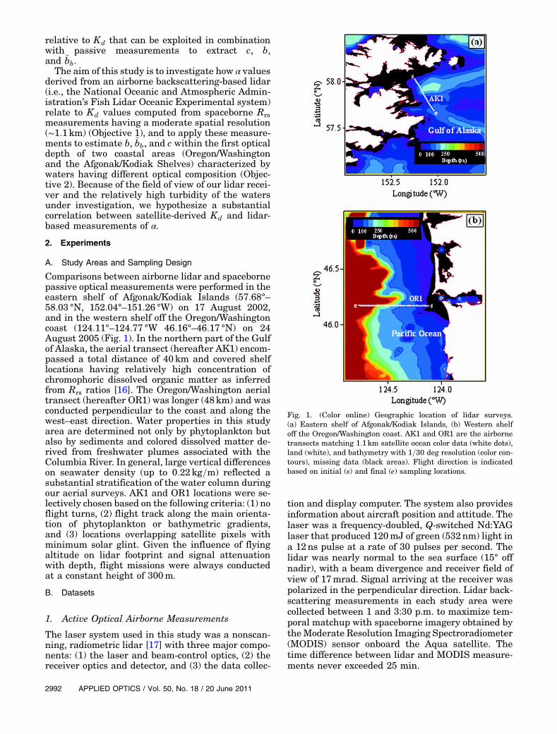
Comparisons between airborne lidar and spacebornepassive optical measurements were performed in theeastern shelf of Afgonak/Kodiak Islands (57:68°–58:03 °N, 152:04°–151:26 °W) on 17 August 2002,and in the western shelf off the Oregon/Washingtoncoast (124:11°–124:77 °W 46:16°–46:17 °N) on 24August 2005 (Fig. 1). In the northern part of the Gulfof Alaska, the aerial transect (hereafter AK1) encom-passed a total distance of 40km and covered shelflocations having relatively high concentration ofchromophoric dissolved organic matter as inferredfrom Rrs ratios [16]. The Oregon/Washington aerialtransect (hereafter OR1) was longer (48km) and wasconducted perpendicular to the coast and along thewest–east direction. Water properties in this studyarea are determined not only by phytoplankton butalso by sediments and colored dissolved matter de-rived from freshwater plumes associated with theColumbia River. In general, large vertical differenceson seawater density (up to 0:22kg=m) reflected asubstantial stratification of the water column duringour aerial surveys. AK1 and OR1 locations were se-lectively chosen based on the following criteria: (1) noflight turns, (2) flight track along the main orienta-tion of phytoplankton or bathymetric gradients,and (3) locations overlapping satellite pixels withminimum solar glint. Given the influence of flyingaltitude on lidar footprint and signal attenuationwith depth, flight missions were always conductedat a constant height of 300m.
B. Datasets
1. Active Optical Airborne Measurements
The laser system used in this study was a nonscan-ning, radiometric lidar [17] with three major compo-nents: (1) the laser and beam-control optics, (2) thereceiver optics and detector, and (3) the data collec-
tion and display computer. The system also providesinformation about aircraft position and attitude. Thelaser was a frequency-doubled, Q-switched Nd:YAGlaser that produced 120mJ of green (532nm) light ina 12ns pulse at a rate of 30 pulses per second. Thelidar was nearly normal to the sea surface (15° offnadir), with a beam divergence and receiver field ofview of 17mrad. Signal arriving at the receiver waspolarized in the perpendicular direction. Lidar back-scattering measurements in each study area werecollected between 1 and 3:30 p.m. to maximize tem-poral matchup with spaceborne imagery obtained bytheModerate Resolution Imaging Spectroradiometer(MODIS) sensor onboard the Aqua satellite. Thetime difference between lidar and MODIS measure-ments never exceeded 25 min.
Fig. 1. (Color online) Geographic location of lidar surveys.(a) Eastern shelf of Afgonak/Kodiak Islands, (b) Western shelfoff the Oregon/Washington coast. AK1 and OR1 are the airbornetransects matching 1:1km satellite ocean color data (white dots),land (white), and bathymetry with 1=30 deg resolution (color con-tours), missing data (black areas). Flight direction is indicatedbased on initial (s) and final (e) sampling locations.
MODIS–Aqua images (local area coverage, Level 2OC, 1:1km footprint) were obtained from NASA(http://oceancolor.gsfc.nasa.gov/). Geo-located, cali-brated, and atmospheric corrected Rrs values wereobtained for spectral bands 9 (438–448nm), 10(483–493nm), 11 (526–536nm), 12 (546–556nm),and 13 (662–672nm), and used to derive inherent op-tical properties (see Subsection 2.C.1). Unlike otherocean color sensors with intermediate spatial resolu-tion (e.g., SeaWiFS), MODIS has a radiometricchannel dedicated to ocean applications centeredat 531nm (i.e., band 11) and spectrally close to thelaser wavelength used in this study. Also, detectionlimits of MODIS are relatively low (e.g., signal/noiseat 490nm∼ twofold) with respect to other sensors.
3. Ancillary Information
Wind speed and direction during the AK1 and OR1surveys were obtained from meteorological stationslocated at the Kodiak Island and Aberdeen airports,respectively (http://www.wunderground.com/). Recei-ver`s radiance contributions due to foam, glint, andbubbles are highly dependent on wind field charac-teristics [18] Therefore, wind information is criticalto quantify these nonwater radiance contributionsand obtain accurate estimates of remotely sensedoptical properties.
C. Processing of Remote Sensing Data
1. Satellite Remote Sensing Reflectance
The operational atmospheric correction for oceancolor products suggested by NASA is based on theGordon and Wang algorithm [19]. The performanceof this model may be compromised in coastal waterslike those investigated here. This issue was exam-ined in our study areas by using the L2 OC flag 12or “TURBIDW.” MODIS-derived total absorptionand backscattering coefficients at 532nm were com-puted based onRrs values at five wavelengths using anew version of the quasi-analytical inversion modelof Lee et al. [20]. Seawater backscattering and ab-sorption coefficients were obtained from Smith andBaker tables [21]. The uncertainty of að532Þ andbbð532Þ estimates using this quasi-analytical para-meterization is about �10% [15]. Kdð532Þ valueswere computed by two methods.
Method I [22]:
Kdð532Þ ≅ ½að532Þ þ bbð532Þ�=μ0; ð4ÞMethod II [14]:
where m0, m1, m2, and m3 are parameters that varywith solar zenith angle and depth interval used toestimate Kd. Unlike Eq. (4), Kd estimates with Meth-od II are calculated with a semiempirical parameter-ization derived from radiative transfer theory [14].
2. Airborne Lidar Backscattering
Raw lidar data in volts were converted to photo-cathode current values based on the specific gainof the photomultiplier. Afterward, the depth of eachlidar sample was found using the surface return as areference, and the return wasmultiplied by a calibra-tion factor to convert photocathode current to lidarvolume backscattering measurements in m−1 sr−1.The calibration factor involves several parametersrelated to geometry (e.g., sampling altitude) and li-dar system characteristics (e.g., pulse energy, areaof receiver).
Calculation of α was performed for each lidar shot,followed by screening and removal of shots contain-ing subsurface scattering layers [23]. The last stepwas necessary to remove the influence of verticalstructure on Kd and α comparisons. For each lidarwaveform, α was computed by linear regression asthe slope between water depth (independent vari-able) and lnðSÞ (dependent variable). This analysiswas performed using full resolution profiles (i.e.,every 0:1m, accuracy ¼ 0:001m) over different depthranges (0–1, 0–5, 0–10, 0–15, 0–20, 2–5, 2–10, 2–15,and 2–20m) to evaluate the influence of surface ef-fects (e.g., bubbles, waves) on Kd − α correlationsand find the optimum vertical interval to matchthe penetration depth of passive sensors (i.e., 1=Kd).Lidar probing depth was estimated as the depth atwhich lidar volume backscattering first fell belowthe level of the background light plus 10 standard de-viations of the noise [23]. Last, we related differencesbetween Kdð532Þ derived from MODIS at 1:1km re-solution with the median, and different averages (ar-ithmetic, geometric, and harmonic) of α value withinthe satellite footprint. This numerical exercise wasintended to examine potential changes of averagedα at 1:1km due to statistical distribution changes.
3. Modeling of b, bb=b, and c
In marine waters with bb=a up to ∼0:25, the diffuseattenuation coefficient of downward irradiance canbe accurately (i.e., ∼5% relative error) approximatedusing a, b, and the solar altitude [7]:
Kd ≅ μ−10 ða2 þGðμ0ÞabÞ0:5; ð6Þ
Gðμ0Þ ¼ 0:425μ0−0:19 for 0 ≤ z ≤ zð0:01Edð0þÞÞ; ð7Þ
where G is a coefficient determining the relativecontribution of scattering to vertical diffuse attenua-tion of irradiance and is defined for a water depth (z)interval coinciding with the euphotic zone, i.e., z atwhich surface downwelling irradiance [Edð0þÞ] is
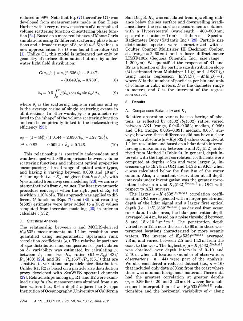
reduced in 99%. Note that Eq. (7) (hereafter G1) wasdeveloped from measurements made in San DiegoHarbor with a very narrow spectrum of b-normalizedvolume scattering function or scattering phase func-tion [24]. Based on amore realistic set of Monte Carlosimulations using 12 different scattering phase func-tions and a broader range of bb=a (0.4–2.6) values, anew approximation for G was found (hereafter G2)[1]. Unlike G1, this model is influenced not only bygeometry of surface illumination but also by under-water light field distribution:
where θs is the scattering angle in radians and ~μSis the average cosine of single scattering events inall directions. In other words, ~μS is a parameter re-lated to the “shape” of the volume scattering functionand can be empirically linked to the backscatteringefficiency [25]:
This relationship is spectrally independent andwas developedwith 869 comparisons between volumescattering functions and inherent optical propertiesencompassing a broad range of optical water types,and having b varying between 0.008 and 10m−1.Assuming that a ≅ Kd and given that b ¼ bb=~bb withbb estimated from inversionmodeling [20],we can cre-ate syntheticb’s from ~bb values. The iterative numericprocedure converges when the right part of Eq. (6)is within�10% of α. This approach was applied to dif-ferent G functions [Eqs. (7) and (8)], and resultingbð532Þ estimates were later added to að532Þ valuescomputed from inversion modeling [20] in order tocalculate cð532Þ.D. Statistical Analysis
The relationship between α and MODIS-derivedKdð532Þ measurements at 1:1km resolution wasquantified using nonparametric Spearman rankcorrelation coefficients (ρs). The relative importanceof size distribution and composition of particulateson ~bb variability was estimated by calculating ρsbetween ~bb and two Rrs ratios (R1 ¼ Rrsð443Þ=Rrsð488Þ [26], and R2 ¼ Rrsð667Þ=Rrsð551Þ) that aresensitive to variations on particle size distribution.Unlike R1, R2 is based on a particle size distributionproxy developed with SeaWiFS spectral channels[27]. Relationships among ~bb, R1, and R2 were exam-ined using in situ measurements obtained from sur-face waters (i.e., 0:6m depth) adjacent to ScrippsInstitution of Oceanography (University of California
San Diego). Rrs was calculated from upwelling radi-ance below the sea surface and downwelling irradi-ance above the sea surface measurements obtainedwith a Hyperspectral (wavelength ¼ 400–800nm,spectral resolution ¼ 1nm) Tethered SpectralRadiometer Buoy (Satlantic Inc.) [28]. Particle sizedistribution spectra were characterized with aCoulter Counter Multisizer III (Beckman Coulter,size range ¼ 2–60 μm) and a laser diffractometerLISST-100x (Sequoia Scientific Inc., size range ¼1–200 μm). We quantified the response of R1 andR2 as a function of the particle size distribution slope(M) estimated from Multisizer III (γ) and LISST (χ)using linear regression [lnðNðDÞÞ ¼ M lnðDÞ þ I,where N is the number of particles per bin and unitof volume in cubic meters, D is the diameter rangein meters, and I is the intercept of the regres-sion curve].
3. Results
A. Comparisons Between α and Kd
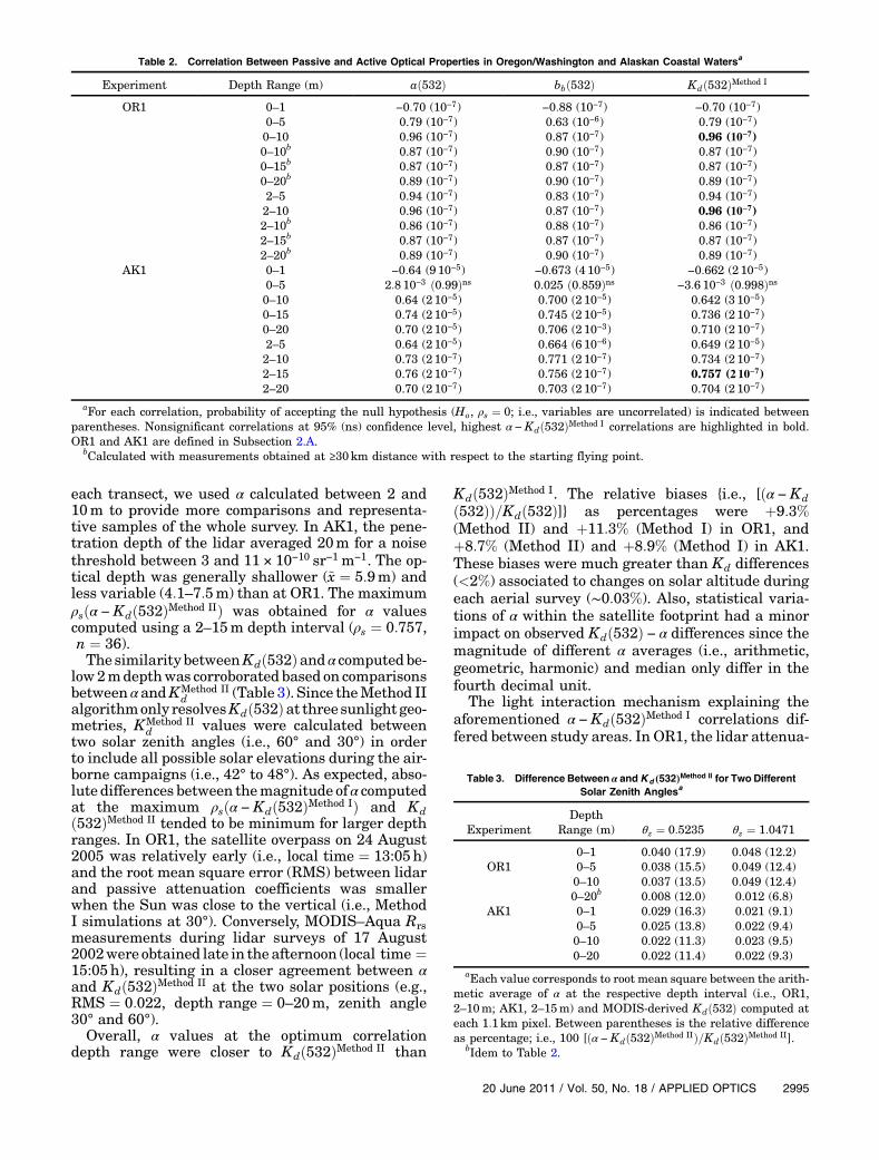
Relative absorption versus backscattering of pho-tons, as reflected by αð532Þ=bbð532Þ ratios, variedbetween AK1 (range, 0.040–0.052; median, 0.046)and OR1 (range, 0.035–0.091; median, 0.057) sur-veys; however, these differences did not have a clearimpact on absolute jα − Kdð532Þj values computed at1:1km resolution and based on a lidar depth intervalhaving a maximum ρs between α and Kdð532Þ as de-rived from Method I (Table 2). In general, depth in-tervals with the highest correlation coefficients werecomputed at depths <5m and were larger (ρs in-creases up to 19.7% in OR1 and 14.3% in AK1) whenα was calculated below the first 2m of the watercolumn. Also, a consistent observation at all depthintervals under investigation was the greater corre-lation between α and Kdð532ÞMethod I in OR1 withrespect to AK1 surveys.
The larger α − Kdð532ÞMethod I correlation coeffi-cient in OR1 corresponded with a larger penetrationdepth of the lidar signal and a larger first opticaldepth (i.e., 1=Kdð532ÞMethod I) as derived from oceancolor data. In this area, the lidar penetration depthaveraged 34:4m, based on a noise threshold between5 and 15 × 10−8 sr−1 m−1. The penetration depthvaried from 12m near the coast to 60m in those wes-ternmost locations characterized by more oceanicwaters. The inverse of Kdð532ÞMethod I averaged7:3m, and varied between 2.5 and 14:3m from thecoast to the west. The highest ρsðα − Kdð532ÞMethod IÞwas obtained over depth intervals of 0–10 and2–10m when all locations (number of observationsobservations ¼ n ¼ 44) were part of the analysis.We also considered a reduced dataset (i.e., n ¼ 16)that included only data ≥30km from the coast wherethere was minimal terrigenous material. These datahad the greatest correlation at greater depths(ρs ¼ 0:89 for 0–20 and 2–20m). However, for a sub-sequent interpretation of α − Kdð532ÞMethod II rela-tionships and the horizontal variability of α along
each transect, we used α calculated between 2 and10m to provide more comparisons and representa-tive samples of the whole survey. In AK1, the pene-tration depth of the lidar averaged 20m for a noisethreshold between 3 and 11 × 10−10 sr−1 m−1. The op-tical depth was generally shallower (~x ¼ 5:9m) andless variable (4:1–7:5m) than at OR1. The maximumρsðα − Kdð532ÞMethod IIÞ was obtained for α valuescomputed using a 2–15m depth interval (ρs ¼ 0:757,n ¼ 36).The similarity betweenKdð532Þandα computedbe-
low2mdepthwas corroborated based on comparisonsbetween α andKMethod II
d (Table 3). Since theMethod IIalgorithmonly resolvesKdð532Þat three sunlight geo-metries, KMethod II
d values were calculated betweentwo solar zenith angles (i.e., 60° and 30°) in orderto include all possible solar elevations during the air-borne campaigns (i.e., 42° to 48°). As expected, abso-lute differences between themagnitude of α computedat the maximum ρsðα − Kdð532ÞMethod IÞ and Kdð532ÞMethod II tended to be minimum for larger depthranges. In OR1, the satellite overpass on 24 August2005 was relatively early (i.e., local time ¼ 13:05h)and the root mean square error (RMS) between lidarand passive attenuation coefficients was smallerwhen the Sun was close to the vertical (i.e., MethodI simulations at 30°). Conversely, MODIS–Aqua Rrsmeasurements during lidar surveys of 17 August2002were obtained late in the afternoon (local time ¼15:05h), resulting in a closer agreement between αand Kdð532ÞMethod II at the two solar positions (e.g.,RMS ¼ 0:022, depth range ¼ 0–20m, zenith angle30° and 60°).
Overall, α values at the optimum correlationdepth range were closer to Kdð532ÞMethod II than
Kdð532ÞMethod I. The relative biases {i.e., [ðα − Kdð532ÞÞ=Kdð532Þ]} as percentages were þ9:3%(Method II) and þ11:3% (Method I) in OR1, andþ8:7% (Method II) and þ8:9% (Method I) in AK1.These biases were much greater than Kd differences(<2%) associated to changes on solar altitude duringeach aerial survey (∼0:03%). Also, statistical varia-tions of α within the satellite footprint had a minorimpact on observed Kdð532Þ − α differences since themagnitude of different α averages (i.e., arithmetic,geometric, harmonic) and median only differ in thefourth decimal unit.
The light interaction mechanism explaining theaforementioned α −Kdð532ÞMethod I correlations dif-fered between study areas. In OR1, the lidar attenua-
Table 2. Correlation Between Passive and Active Optical Properties in Oregon/Washington and Alaskan Coastal Watersa
Experiment Depth Range (m) að532Þ bbð532Þ Kdð532ÞMethod I
aFor each correlation, probability of accepting the null hypothesis (Ho, ρs ¼ 0; i.e., variables are uncorrelated) is indicated betweenparentheses. Nonsignificant correlations at 95% (ns) confidence level, highest α −Kdð532ÞMethod I correlations are highlighted in bold.OR1 and AK1 are defined in Subsection 2.A.
bCalculated with measurements obtained at ≥30km distance with respect to the starting flying point.
Table 3. Difference Between α andKd �532�Method II for Two DifferentSolar Zenith Anglesa
aEach value corresponds to root mean square between the arith-metic average of α at the respective depth interval (i.e., OR1,2–10m; AK1, 2–15m) and MODIS-derived Kdð532Þ computed ateach 1:1km pixel. Between parentheses is the relative differenceas percentage; i.e., 100 [ðα − Kdð532ÞMethod IIÞ=Kdð532ÞMethod II].
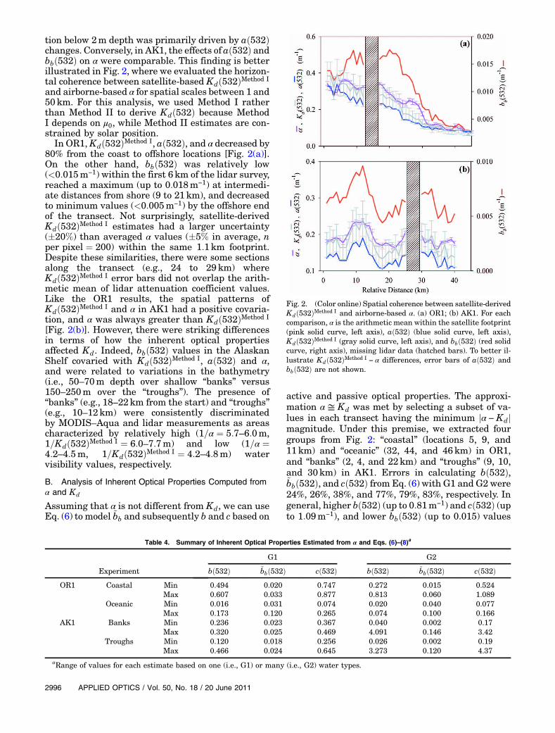
tion below 2m depth was primarily driven by að532Þchanges. Conversely, in AK1, the effects of að532Þ andbbð532Þ on α were comparable. This finding is betterillustrated in Fig. 2, where we evaluated the horizon-tal coherence between satellite-based Kdð532ÞMethod I
and airborne-based α for spatial scales between 1 and50km. For this analysis, we used Method I ratherthan Method II to derive Kdð532Þ because MethodI depends on μ0, while Method II estimates are con-strained by solar position.
In OR1,Kdð532ÞMethod I, að532Þ, and α decreased by80% from the coast to offshore locations [Fig. 2(a)].On the other hand, bbð532Þ was relatively low(<0:015m−1) within the first 6km of the lidar survey,reached a maximum (up to 0:018m−1) at intermedi-ate distances from shore (9 to 21km), and decreasedto minimum values (<0:005m−1) by the offshore endof the transect. Not surprisingly, satellite-derivedKdð532ÞMethod I estimates had a larger uncertainty(�20%) than averaged α values (�5% in average, nper pixel ¼ 200) within the same 1:1km footprint.Despite these similarities, there were some sectionsalong the transect (e.g., 24 to 29km) whereKdð532ÞMethod I error bars did not overlap the arith-metic mean of lidar attenuation coefficient values.Like the OR1 results, the spatial patterns ofKdð532ÞMethod I and α in AK1 had a positive covaria-tion, and α was always greater than Kdð532ÞMethod I
[Fig. 2(b)]. However, there were striking differencesin terms of how the inherent optical propertiesaffected Kd. Indeed, bbð532Þ values in the AlaskanShelf covaried with Kdð532ÞMethod I, að532Þ and α,and were related to variations in the bathymetry(i.e., 50–70m depth over shallow “banks” versus150–250m over the “troughs”). The presence of“banks” (e.g., 18–22km from the start) and “troughs”(e.g., 10–12km) were consistently discriminatedby MODIS–Aqua and lidar measurements as areascharacterized by relatively high (1=α ¼ 5:7–6:0m,1=Kdð532ÞMethod I ¼ 6:0–7:7m) and low (1=α ¼4:2–4:5m, 1=Kdð532ÞMethod I ¼ 4:2–4:8m) watervisibility values, respectively.
B. Analysis of Inherent Optical Properties Computed fromα and Kd
Assuming that α is not different from Kd, we can useEq. (6) to model ~bb and subsequently b and c based on
active and passive optical properties. The approxi-mation α ≅ Kd was met by selecting a subset of va-lues in each transect having the minimum jα − Kdjmagnitude. Under this premise, we extracted fourgroups from Fig. 2: “coastal” (locations 5, 9, and11km) and “oceanic” (32, 44, and 46km) in OR1,and “banks” (2, 4, and 22km) and “troughs” (9, 10,and 30km) in AK1. Errors in calculating bð532Þ,~bbð532Þ, and cð532Þ from Eq. (6) with G1 and G2 were24%, 26%, 38%, and 77%, 79%, 83%, respectively. Ingeneral, higher bð532Þ (up to 0:81m−1) and cð532Þ (upto 1:09m−1), and lower ~bbð532Þ (up to 0.015) values
Fig. 2. (Color online) Spatial coherence between satellite-derivedKdð532ÞMethod I and airborne-based α. (a) OR1; (b) AK1. For eachcomparison, α is the arithmetic mean within the satellite footprint(pink solid curve, left axis), að532Þ (blue solid curve, left axis),Kdð532ÞMethod I (gray solid curve, left axis), and bbð532Þ (red solidcurve, right axis), missing lidar data (hatched bars). To better il-lustrate Kdð532ÞMethod I
− α differences, error bars of að532Þ andbbð532Þ are not shown.
Table 4. Summary of Inherent Optical Properties Estimated from α and Eqs. (6)–(8)a
were estimated in OR1 than in AK1 (Table 4). InOR1, the “coastal” group was characterized by higherbð532Þ (up to tenfold) and cð532Þ (up to sevenfold)and lower ~bbð532Þ (up to 0.4-fold) values than thosefor the “oceanic” group. Shallower waters of AK1 as-sociated with submarine banks had typically lowerbð532Þ (up to 0:24m−1) and cð532Þ (up to 0:37m−1)and higher ~bbð532Þ (up to 0.025) values than thoseover deep canyons (i.e., “troughs”).
The concurrent use of active and optical passivemeasurements in this study was also applied toestimate second-order optical attributes affecting
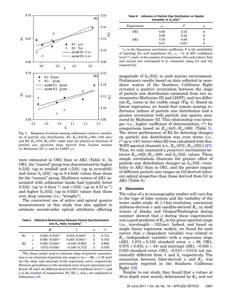
magnitude of ~bbð532Þ in each marine environment.Preliminary results based on data collected in near-shore waters of the Southern California Bightrevealed a positive covariation between the slopeof particle size distribution estimated from two in-struments (Multisizer III and LISST), and two differ-ent Rrs ratios in the visible range (Fig. 3). Based onlinear regression, we found that remote sensing re-flectance indices of particle size distribution had agreater covariation with particle size spectra mea-sured by Multisizer III. This relationship was stron-ger (i.e., higher coefficient of determination, r2) forcomparisons based on Rrsð443Þ=Rrsð488Þ (Table 5).The lower performance of R2 for detecting changeson particle size distribution was even worse (i.e.,r2 up to 14% lower) when R2was calculated with Sea-WiFS spectral channels [i.e., Rrsð670Þ=Rrsð555Þ] [27].Thus, we only examined a posteriori correlations be-tween Rrsð443Þ=Rrsð488Þ and ~bbð532Þ values. Thesesimple correlations illustrate the greater effect ofparticle size distribution changes on ~bbð532Þ varia-bility in AK1 than in OR1, and the greater impactof different particle size ranges on G2-derived inher-ent optical properties than those derived from G1 inAK1 (Table 6).
4. Discussion
The value of α in oceanographic studies will vary dueto the type of lidar system and the turbidity of thewater under study. At 1:1km resolution, concurrentairborne-derived α and satellite-derived Kd in shelfwaters of Alaska and Oregon/Washington duringsummer showed that α during these experimentswas a good predictor ofKd in the green spectral range(i.e., wavelength ¼ 532nm). Indeed, and based onsingle linear regression models, we found for eachsurvey that α (dependent variable) was related toKd (independent variable) with a regression slope(AK1, 1:074� 0:132 standard error, n ¼ 36; OR1,0:975� 0:053, n ¼ 44) and intercept (AK1, −0:030�0:025 standard error; OR1, −0:013� 0:013) not sta-tistically different from 1 and 0, respectively. Theconnection between lidar-derived α and Kd waspreviously reported in the Southern CaliforniaBight [10].
Similar to our study, they found that α values at20m depth were mainly determined by Kd and not
Table 6. Influence of Particle Size Distribution on SpatialVariability of ~bb �532�a
Experiment ρs P n
OR1 0.60 0.24 60.60 0.24 6
AK1 0.78 0.06 60.87 0.03* 6
aρs is the Spearman correlation coefficient, P is the probabilityof rejecting the null hypothesis (Ho, ρs ¼ 0) at 95% confidencelevel (*), and n is the number of comparisons. For each subset, firstand second row correspond to ~bb estimates using G1 and G2,respectively.
Table 5. Statistical Relationships Between Particle Size Distributionand Rrs Ratio Variabilitya
aThe linear model used to estimate slope of particle concentra-tion (y) as a function of particle size range (x) is y ¼ Mxþ I;M and Iare the slope and intercept of the regression curve, respectively.Between parentheses is the standard error of each regression coef-ficient,M and I are different from 0 at 95% confidence level (*), andn is the number of comparisons. R1, R2, γ, and χ are explained inSubsection 2.D.
Fig. 3. Response of remote sensing reflectance ratios to variabil-ity of particle size distribution. R1, Rrsð443ÞRrsð488Þ (left axis)and R2, Rrsð670Þ=Rrsð555Þ (right axis) are plotted as functions ofparticle size spectrum slope derived from Coulter counter(a) Multisizer III (γ) and (b) LISST (χ).
c (see linear regression slope of Eqs. 5 and 6 in [10]).However, in contrast with our findings, their α − Kdregression slope was below unity. We attribute thisapparent discrepancy to differences in cR. In theSouthern California Bight study [10], the laser beamdivergence angle (43mrad) and receiver field of view(26mrad) were larger with respect to our study, andlidar measurements were obtained from the shipdeck (i.e., distance between lidar source/detector andsea surface was 10:3m). Given this geometry, their R(∼0:08m) and cR (∼0:01) values were relatively smallcompared with our values (R ∼ 2:5m, cR ∼ 1). There-fore, as cR becomes smaller than 1 (i.e., Churnsideet al.’s study [10]), c is expected to explain a largerfraction of Kd [29]. Another variable decreasing cRin contribution [10] was their lower cð532Þ values(mean ¼ 0:098m−1) with respect to our study (AK1,0:173m−1; OR1, 0:193m−1). Note that Kd and c deter-minations by [10] weremore accurate than ours sincethey were derived from in-water measurements.Finally, it is worth emphasizing that our lidar resultsare based on cross-polarized lidar returns, while thestudy in [10] describes values for the copolarized re-turns. Multiple forward scattering can produce a re-duced attenuation of the cross-polarized returnsunder some conditions [30].
Despite the overall agreement between magnitudeof α and MODIS-derived Kdð532Þ measurementsduring the AK1 and OR1 surveys, we detected sub-stantial changes (up to þ0:088 in OR1 and þ0:049 inAK1) between these two properties at specific loca-tions along the transects (e.g., 26–28km in OR1,18km in AK1). Since α values lie between c andKd [8–10] and c is always larger than Kd, it is sug-gested that the observed increase of α with respectto the Kdð532Þmagnitude was associated in these lo-cations with a larger relative contribution of cð532Þto α, and, consequently, a greater proportion of for-ward scattering defining the underwater light field.We attribute these spatial changes (i.e., within andbetween transects) to the presence of different opti-cal water types.
Although averaged hourly wind speed was higherduring the OR1 survey (4:44ms−1) than during theAK1 survey (3:33ms−1), its influence on α − Kdð532Þdifferences was secondary due to three main reasons.First, and based on other studies [31], the greaterwind intensity and associated production of subsur-face bubbles in Oregon/Washington is expected tohave a minor impact on lidar volume backscattering(∼25%) compared to observed relative changesbetween α and Kdð532Þ (up to 60%). Second, our α −
Kdð532Þ comparisons were based on α calculated be-low 2m depth, thus eliminating major interferencedue to “surface” effects. This interference was morepronounced when Kdð532Þ was estimated withMethod I since the Method II approach was devel-oped using constant and relatively weak winds(i.e., 5ms−1). Last, the influence of wind-mediatedchanges on sea surface slopes (cross and up/down)and subsequent contribution of Sun glint to Rrs
was ruled out as a possible major bias of Kdð532Þestimates since the specific radiance threshold at865nm proposed for MODIS–Aqua (i.e., flagMODGLINT or moderate Sun glint contamination)was never exceeded during the analysis of oceancolor data.
For a specific range of oceanographic conditionsand lidar system parameters, active and passive op-tical measurements were combined in this study tocalculate inherent optical properties related to mag-nitude and angular distribution of light scattering.Values of bð532Þ, cð532Þ, and ~bbð532Þ can also be es-timated by making equal Eqs. (5) and (6) and solvingfor b. However, this mathematical procedure hassome drawbacks. First, the use of two models is add-ing more error (∼12%) to the final estimates. Second,Kd models based on passive optical measurementsare based on bb=a changes, thus forward scatteringcontributions are not quantified. The median ofbð532Þ (n ¼ 3) in OR1 (G1, 0:49m−1) and AK1 (G1,0:36m−1) as estimated from G1 was within the rangeof oceanic (0:275m−1) and coastal (1.21 to 1:82m−1)values reported at the same wavelength in SouthernCalifornia waters [24]. Our G1-based cð532Þ esti-mates (median in OR1, 0:55m−1; AK1. 0:48m−1) werealso intermediate between oligotrophic (e.g., 0:2m−1)and eutrophic (e.g., up to 10m−1) marine environ-ments [32]. Unlike bð532Þ and cð532Þ, our estimatesof backscattering probability at 532nm were some-times beyond (e.g., oceanic in OR1, G2-based inAK1) the maximum ~bb values measured in the Paci-fic Central Gyre (0.04–0.06) [13] and the BahamasShelf during a “whiting event” (∼0:05) [12]. Giventhe relative low signal in our oceanic locations andthe high uncertainty (relative error up to 79%) of~bbð532Þ estimates using more realistic volume scat-tering functions (i.e., G2), we suggest that observedvariations of ~bbð532Þwith respect to literature valueswere apparent. The use of multiple and different op-tical signals in this research allowed us not only toquantify a budget of inherent optical propertiesbut also to investigate additional physical aspects re-lated to ~bb behavior due to variations on particle sizedistribution. In that regard, the substantial and ex-clusive correlation found between G2-based ~bb andRrsð443Þ=Rrsð488Þ in AK1 is indirectly suggestingtwo important facts: the more heterogeneous natureof the volume scattering function in AK1with respectto OR1, and the greater importance of other factors(e.g., changes on particle composition due to riversediments) affecting backscattering efficiency duringOR1 surveys.
This work was supported by the Naval ResearchLaboratory (NRL) internal project “3D RemoteSensing with a Multiple-Band Active and PassiveSystem: Theoretical Basis,” PBE0601153N.
References1. J. T. O. Kirk, “Volume scattering function, average cosines, and
the underwater light field,” Limnol. Oceanogr. 36, 455–467(1991).
2. Z. Lee, A. Weidemann, J. Kindle, R. Arnone, K. Carder, andC. Davis, “Euphotic zone depth: its derivation and implicationto ocean-color remote sensing,” J. Geophys. Res. 112, C03009(2007).
3. M. R. Lewis, M. E. Carr, G. C. Feldman, E. Wayne, andC. McClain, “Influence of penetrating solar radiation on theheat budget of the equatorial Pacific Ocean,” Nature 347,543–545 (1990).
4. Ø. Varpe and Ø. Fiksen, “Seasonal plankton-fish interactions:light regime, prey phenology, and herring foraging,” Ecology91, 311–318 (2010).
5. R. P. Dunne and B. E. Brown, “Penetration of solar UVB ra-diation in shallow tropical waters and its potential biologicaleffects on coral reefs; results from the central Indian Oceanand Andaman Sea,”Mar. Ecol. Prog. Ser. 144, 109–118 (1996).
6. M. A. Montes-Hugo, S. Alvarez-Borego, and A. Giles-Guzmán,“Horizontal sighting range and Sechii depth as estimators ofunderwater PAR attenuation in a coastal lagoon,” Estuaries26, 1302–1309 (2003).
7. J. T. O. Kirk, “Dependence of relationship between inherentand apparent optical properties of water and solar altitude,”Limnol. Oceanogr. 29, 350–356 (1984).
8. H. R. Gordon, “Interpretation of airborne oceanic lidar: effectsof multiple scattering,” Appl. Opt. 21, 2996–3001 (1982).
9. R. E. Walker and J. W. McLean, “Lidar equations for turbidmedia with pulse stretching,” Appl. Opt. 38, 2384–2397(1999).
10. J. H. Churnside, V. T. Viatcheslav, and J. J. Wilson, “Oceano-graphic lidar attenuation coefficients and signal fluctuationsmeasured from a ship in the Southern California Bight,” Appl.Opt. 37, 3105–3111 (1998).
11. H. R. Gordon, “Sensitivity of radiative transfer to small-anglescattering in the ocean: quantitative assessment,” Appl. Opt.32, 7505–7511 (1993).
12. H. M. Dierssen, R. C. Zimmerman, and D. J. Burdige, “Opticsand remote sensing of Bahamian carbonate sediment whitingand potential relationship to wind-driven Langmuir circula-tion,” Biogeosciences 6, 487–500 (2009).
13. M. S. Twardowski, H. Claustre, S. A. Freeman, D. Stramski,and Y. Huot, “Optical backscattering properties of the ‘clear-est’ natural waters,”Biogeosciences Disc. 4, 2441–2491 (2007).
14. Z. Lee, K. P. Du, and R. Arnone, “A model for the diffuse at-tenuation coefficient of downwelling irradiance,” J. Geophys.Res. 110, C02016 (2005).
15. Z. Lee, R. Arnone, C. Hu, J. Werdell, and B. Lubac, “Uncertain-ties of optical parameters and their propagations in an analy-tical ocean color inversion algorithm,” Appl. Opt. 49, 369–381(2010).
16. M. A. Montes-Hugo, K. Carder, R. J. Foy, J. Canizzaro,E. Brown, and S. Pegau, “Estimating phytoplankton biomassin coastal waters of Alaska using airborne remote sensing,”Remote Sens. Environ. 98, 481–493 (2005).
17. J. H. Churnside, J. J. Wilson, and V. V. Tatarski, “Airbornelidar for fisheries application,” Opt. Eng. 40, 406–414 (2001).
18. J. H. Churnside and J. J. Wilson, “Ocean color inferred fromradiometers on low-flying aircraft,” Sensors 8, 860–876 (2008).
19. H. R. Gordon and M. Wang, “Retrieval of water-leavingradianceandaerosolopticalthicknessovertheoceanswithSea-WiFS: apreliminaryalgorithm,”Appl.Opt.33, 443–552 (1994).
20. Z. Lee, B. Lubac, J. Werdell, and R. Arnone, “An update of thequasi-analytical algorithm (QAA_v5),” in International OceanColor Group Software Report (2009), www.ioccg.org/groups/Software_OCA.
21. R. C. Smith and K. S. Baker, “Optical properties of the clearestnatural waters (200–800nm),” Appl. Opt. 20, 177–181 (1981).
22. S. Sathyendranath and T. Platt, “The spectral irradiance fieldat the surface and in the interior of the ocean: a model forapplications in oceanography and remote sensing,” J.Geophys. Res. 93, 9270–9280 (1988).
23. M. A. Montes-Hugo, J. H. Churnside, R. W. Gould, R. A.Arnone, and R. Foy, “Spatial coherence between remotelysensed ocean color data and vertical distribution of lidar back-scattering in coastal stratified waters,” Remote Sens. Environ.114, 2584–2593 (2010).
24. T. J. Petzold, “Volume scattering functions for selected oceanwaters,” SIO ref. 72–78, Scripps Institution of Oceanography,La Jolla, California, 1972.
25. V. I. Haltrin, M. E. Lee, V. I. Mankovsky, E. B. Shybanov, andA. D. Weidemann, “Integral properties of angular light scat-tering coefficient measured in various natural waters,” in Pro-ceedings of the II International Conference Current Problemsin Optics of Natural Waters, I. Levin and G. Gilbert, eds.(2003), pp. 252–257.
26. K. L. Carder, F. R. Chen, Z. P. Lee, and S. K. Hawes, “Semi-analytical Moderate-Resolution Imaging Spectrometer algo-rithms for chlorophyll a and absorption with bio-opticaldomains based on nitrate-depletion temperatures,” J.Geophys. Res. 104, 5403–5421 (1999).
27. E. J. D’Sa and D. S. Ko, “Short-term influences on suspendedparticulatematter distribution in the northernGulf of Mexico:satellite and model observations,” Sensors 8, 4249–4264(2008).
28. P. Wang, E. S. Boss, and C. Roesler, “Uncertainties of inherentoptical properties obtained from semianalytical inversions ofocean color,” Appl. Opt. 44, 4074–4085 (2005).
29. Y. I. Kopelevich and A. G. Surkov, “Mathematical modeling ofthe input signals of oceanographic lidars,” J. Opt. Technol. 75,321–326 (2008).
30. J. H. Churnside, “Polarization effects on oceanographic lidar,”Opt. Express 16, 1196–1207 (2008).
31. J. H. Churnside, “Lidar signature from bubbles in the sea,”Opt. Express 18, 8294–8299 (2010).
32. J. R. Zanaveld and S. Pegau, “Robust underwater visibilityparameter,” Opt. Express 11, 2997–3009 (2003).