Relativistic light-matter interaction Tor Kjellsson Abstract: In this licentiate thesis light-matter interaction between hydrogen and superintense attosecond pulses is studied. The specific aim here is to identify for what intensities the non-relativistic calculations, given by solving the time dependent Schrödinger equation, no longer are valid. In order to do this the time dependent Dirac equation has been numerically solved for interaction beyond the so called dipole approximation, where spatial dependence of the pulse is neglected. The spatial part of the pulse is taken into account by a power series expansion truncated at a certain order. It is shown that the relativistic description demands more terms in this expansion compared to the non-relativistic description. As spatial dependence is computationally heavy to take into account, several optimizations have been made. As relativistic effects are expected when the classical quiver velocity of the electron reaches a substantial fraction of the speed of light, this thesis considers cases up to v ≈ 0.23 c Akademisk avhandling för avläggande av licentiatexamen vid Stockholms universitet, Fysikum Licentiatseminariet äger rum 28 september kl.10 i sal FB55, Fysikum, Albanova universitetscentrum, Roslagstullsbacken 21, Stockholm.
Transcript
Relativistic light-matter interaction
Tor Kjellsson
Abstract:
In this licentiate thesis light-matter interaction between hydrogen and superintense attosecond pulses is studied. The specific aim here is to identify for what intensities the non-relativistic calculations, given by solving the time dependent Schrödinger equation, no longer are valid. In order to do this the time dependent Dirac equation has been numerically solved for interaction beyond the so called dipole approximation, where spatial dependence of the pulse is neglected.
The spatial part of the pulse is taken into account by a power series expansion truncated at a certain order. It is shown that the relativistic description demands more terms in this expansion compared to the non-relativistic description. As spatial dependence is computationally heavy to take into account, several optimizations have been made.
As relativistic effects are expected when the classical quiver velocity of the electron reaches a substantial fraction of the speed of light, this thesis considers cases up to v≈0.23c
Akademisk avhandling för avläggande av licentiatexamen vid Stockholms universitet, Fysikum
Licentiatseminariet äger rum 28 september kl.10 i sal FB55, Fysikum, Albanova universitetscentrum, Roslagstullsbacken 21, Stockholm.
1
Relativistic light-matter interaction
Tor Kjellsson
Akademisk avhandling for avläggande av licentiatexamen i teoretisk fysikvid Stockholms Universitet, september 2015
In this licentiate thesis light-matter interaction between hydrogen and superintense attosecondpulses is studied. The specific aim here is to identify for what intensities the non-relativisticcalculations, given by solving the time dependent Schrödinger equation, no longer are valid. Inorder to do this the time dependent Dirac equation has been numerically solved for interactionbeyond the so called dipole approximation, where spatial dependence of the pulse is neglected.
The spatial part of the pulse is taken into account by a power series expansion truncated at acertain order. It is shown that the relativistic description demands more terms in this expansioncompared to the non-relativistic description. As spatial dependence is computationally heavy totake into account, several optimizations have been made.
As relativistic effects are expected when the classical quiver velocity of the electron, vquiv,reaches a substantial fraction of the speed of light, this thesis considers cases up to vquiv ≈ 0.23c.
PAPER I: Relativistic ionization dynamics for a hydrogen atom exposed to super-intenseXUV laser pulsesTor Kjellsson, Sølve Selstø, Eva LindrothIn manuscript
2.1 Energy spectrum for κ = −1. In this case, there are 183 values in total, onefor each basis element in the model space. The model spectrum splits into twosubsets and towards the extreme values the discrete nature of the model spectrumis seen. . . . . . . . . . . . . . . . . . . . . . . . . . . . . . . . . . . . . . . . . . . 24
2.2 The first few eigenvalues of the positive energy spectrum for κ = −1. . . . . . . . 25
2.3 Probability distribution for the two radial components of the ground state. TheQ-component has been multiplied by a factor of 100. . . . . . . . . . . . . . . . 26
3.1 Comparison of mathematical model (blue) with experimentally produced pulse(red). The bottom figure is adapted from [1]. . . . . . . . . . . . . . . . . . . . . 32
4.1 Radial probability of an electron initially in the ground state. The pulse it inter-acts with is a sine-square pulse with ω = 3.5 a.u and E0 = 10 a.u. The times aregiven in percentage of the pulse length with zero field strength after 100%. . . . 45
4.2 Radial probability of an electron initially in the ground state. Here E0 = 60 a.u.while the other pulse parameters are the same as in Fig. 4.1. . . . . . . . . . . . . 46
4.3 Radial probability of an electron initially in the ground state. The field strengthhere is E0 =10 a.u. In the left figure uniform scaling has been employed while theright figure presents dynamics with exterior complex scaling, both with θ = 10degrees. The black dashed line indicates where the rotation starts. . . . . . . . . 47
4.4 Relativistiv couplings matrices. Each coloured block denotes a coupling of thecorrsponding operator between two states. In general, the operator contains a lofof zero entries and as such is said to be sparse. . . . . . . . . . . . . . . . . . . . 49
4.5 A comparison between the full BYD3 angular couplings with the reduced matrixelements not duplicated. The left figure can be reproduced from the right by justmultiplication of the correct angular factor. . . . . . . . . . . . . . . . . . . . . . 50
4.6 Probability to find the electron in the ground state as a function of time. Thepulse here has a total time of T = 30π a.u, E0 = 40.0 a.u and ω = 3.5 a.u. Thedots are the results from dynamics with full coupling matrices while the red solidline is an optimized Krylov implementation. . . . . . . . . . . . . . . . . . . . . . 51
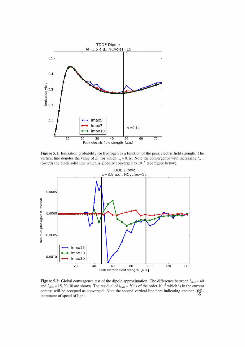
5.1 Ionization probability for hydrogen as a function of the peak electric field strength.The vertical line denotes the value of E0 for which vq ≈ 0.1c. Note the conver-gence with increasing lmax towards the black solid line which is globally con-verged to 10−5 (see figure below). . . . . . . . . . . . . . . . . . . . . . . . . . . . 55
5.2 Global convergence test of the dipole approximation. The difference betweenlmax = 40 and lmax = 15,20,30 are shown. The residual of lmax = 30 is of the order10−5 which is in the current context will be accepted as converged. Note thesecond vertical line here indicating another 10%-increment of speed of light. . . 55
5.3 Comparison of TDSE and TDDE calculation (lmax = 40) within the dipole ap-proximation. At vq ≈ 0.15c, the non-relativistic Pion starts to increase comparedto the relativistic Pion. . . . . . . . . . . . . . . . . . . . . . . . . . . . . . . . . . 56
5.4 Pion predicted by TDSE within (dashed line) and beyond (solid line) dipole ap-proximation. The acronym BYD1 stands for first order beyond dipole approxi-mation. . . . . . . . . . . . . . . . . . . . . . . . . . . . . . . . . . . . . . . . . . . 57
5.5 Comparison of TDDE and TDSE in the non-relativistic regime. The numberstrailing the acronym "BYD" are the numerical value of N in eq. 5.2. For allcases lmax = 15 has been used which in this region is enough for convergence. . . 58
5.6 The radial probability distributions of the electron initially in the ground state.The percentage refers to elapsed interaction time. While BYD2 and BYD3 areoverlapping after the pulse the wavefunction following the BYD1 Hamiltonianis visibly different. The peak electric field strength is here E0 = 40.0 a.u. . . . . . 59
5.7 A comparison of Pion computed with and without the time independent negativeenergy states in the basis. . . . . . . . . . . . . . . . . . . . . . . . . . . . . . . . 60
5.8 Pion for TDDE BYD3. For E0 > 80 a.u. lmax > 15 is requred while for E0 > 100a.u. lmax > 20 is required for convergence. . . . . . . . . . . . . . . . . . . . . . . 61
6.1 B-splines of orders k = 2,3,4,7 on the sequence 0,1,2,3,4. Note that orderk implies piecewise polynomials of order k−1, clearly visible k = 1,2. At eachvalue r the B-splines sum up to unity, reflecting their completeness. . . . . . . . lxvi
List of Tables
2.1 The set of quantum numbers (omitting m j) that are related to each other for therelativistic eigenfunctions. . . . . . . . . . . . . . . . . . . . . . . . . . . . . . . . 26
2.2 The four lowest eigenvalues belonging to the positive energy spectrum for thestate lP = 1, j = 1/2. When using k1 = k2 the lowest eigenvalue in the positive setis identical to the ground state for which lP = 0. . . . . . . . . . . . . . . . . . . . 27
4.1 Comparing figures for full and Krylov implementation. The model space hereconsists of 2 × 20 B-splines per angular symmetry, with 128 such included.(lmax = 7). . . . . . . . . . . . . . . . . . . . . . . . . . . . . . . . . . . . . . . . . 51
5.1 Grid parameters for model box. The same equidistant knot sequence is used forTDSE and TDDE computation. Note that the relativistic computations requiretwice as many radial states due to having two components. Since the angularbasis is twice as large due to spin, the relativistic basis is four times larger thanthe non-relativistic basis for the same box and lmax. . . . . . . . . . . . . . . . . . 54
6.1 Conversion table for physical quantities. α is the fine structure constant, as it isdimensionless it has the same value in atomic units as in SI-units. . . . . . . . . lxv
1. Introduction
Prediction is very difficult, especially about the future - Niels Bohr
There seem to be rules by which nature abides when the current state of «everything»evolves. The scientific community is not only trying to find these rules but also comprehendthem, ultimately to a level where they perhaps can be applied to benefit society. The past centurypresented a series of triumphs of this kind, with applications for instance of special and generalrelativity to calibrate GPS-systems and the use of quantum mechanics for medical imaging.
One widely used method to obtain information about a system is to study its interactionwith light. It may be applied on the very largest of systems such as stars, galaxies and even theuniverse itself, as well as on the tiny systems of microcosm: the world of molecular and atomicsystems.
On the microscopic scales the rules are given by quantum mechanics. In this theory a systemtypically evolves on the time scale Tsc given by:
e−i ∆E⋅th → Tsc ∼
h∆E
(1.1)
where ∆E = E f in −Ein is the energy difference between an initial and final state. For an atomicsystem ∆E ≈ eV giving a time scale of:
Tatom ∼ 10−16s. (1.2)
Recent advances in laser technology have now progressed the field to a point where subfemtosec-ond laser pulses, also called attosecond pulses can be generated. These have a time resolutionon the scale of 10−18s, thus enabling the study of electronic motion in atoms on its natural timescale [2]. With this experimental opportunity, theoretical predictions for dynamics on this scalemay be tested.
The development has not just made pulses short enough to monitor dynamics but alsostrong enough to influence it. While the intensity of the Z = 1 Coulomb field at one bohr ra-dius is Ic ∼ 1016W/cm2, pulses with peak intensities as high as I ∼ 1022W/cm2 have beenreported [3]. Although pulses with this intensity have not yet been used in experiments, theo-retical efforts have been made to study light-matter interaction in the relativistic regime whereIrel > 1018W/cm2 [4] and even beyond that [5]. However, due to the extremely challenging na-ture of phenomena occurying in these regimes most studies are carried out in simplified models.
In this thesis light-matter interaction is studied within the fully relativistic description given bythe time dependent Dirac equation (TDDE). Although there exist some work in this field [6–9]
13
there is to our knowledge no work that, in a full-dimensional calculation, incorporates more thanthe lowest order relativistic interaction for a realistic pulse type and problem size. In order to dothis here, the focus is put on the interaction itself by studying one electron systems interactingwith external electromagnetic fields.
14
2. The hydrogen atom
The purpose of computing is insight, not numbers - Richard Hamming
One electron systems are of fundamental importance since they are the only atomic system forwhich the electronic structure can be solved exactly. In quantum mechanics a system is char-acterized by its state ∣Ψ(t)⟩ and in coordinate space, information about the system is availablein the wave function Ψ(r,t) = ⟨r∣Ψ(t)⟩. The evolution of the wave function is governed by theequation of motion:
ih∂Ψ(r,t)
∂ t= H(t)Ψ(r,t) (2.1)
where the Hamiltonian H(t) contains all operators associated with energy within the chosenframework. In subsequent chapters eq. 2.1 is solved for a non-relativistic and relativistic Hamil-tonian to compare when the relativistic effects starts influencing the dynamics.
At any point in time the set of eigenfunctions Φ(r,t) of H(t) span the Hilbert space of Ψ(r,t)and can thus be used as a basis to work in. In this work the time dependent wave function Ψ(r,t)will be spectrally decomposed in the set of eigenfunctions Φ(r) of the Hamiltonian prior toany interaction: H(t = 0) = H0.
The next sections cover the basics of finding this basis and how to represent it in a practicalcalculation. Once the basis is computed eq. 2.1 can be addressed for an external field.
2.1 Non-relativistic spectrum
For hydrogen, assuming a non-relativistic description with a point-like nucleus of infinite massthe Hamiltonian is [10];
H0 =p ⋅p2m
− e2
4πε0r(2.2)
where p is the canonical momentum, e the electric charge, m the electron mass, ε0 the permittiv-ity of free space and r the distance to the nucleus. To see that this Hamiltonian consists of termsassociated with energy, note that the last term in eq 2.2 is the Coulomb potential while the firstterm represents the classical kinetic energy:
Ekin =mv2
2= p2
2m(2.3)
15
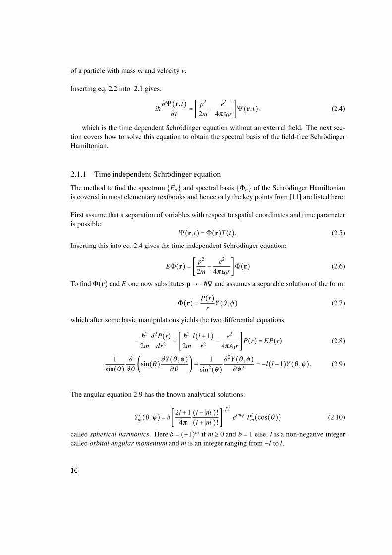
of a particle with mass m and velocity v.
Inserting eq. 2.2 into 2.1 gives:
ih∂Ψ(r,t)
∂ t= [ p2
2m− e2
4πε0r]Ψ(r,t) . (2.4)
which is the time dependent Schrödinger equation without an external field. The next sec-tion covers how to solve this equation to obtain the spectral basis of the field-free SchrödingerHamiltonian.
2.1.1 Time independent Schrödinger equation
The method to find the spectrum En and spectral basis Φn of the Schrödinger Hamiltonianis covered in most elementary textbooks and hence only the key points from [11] are listed here:
First assume that a separation of variables with respect to spatial coordinates and time parameteris possible:
Ψ(r,t) =Φ(r)T(t). (2.5)
Inserting this into eq. 2.4 gives the time independent Schrödinger equation:
EΦ(r) = [ p2
2m− e2
4πε0r]Φ(r) (2.6)
To find Φ(r) and E one now substitutes p→ −h∇∇∇ and assumes a separable solution of the form:
Φ(r) = P(r)r
Y(θ ,φ) (2.7)
which after some basic manipulations yields the two differential equations
− h2
2md2P(r)
dr2 +[ h2
2ml(l+1)
r2 − e2
4πε0r]P(r) = EP(r) (2.8)
1sin(θ)
∂
∂θ(sin(θ)∂Y(θ ,φ)
∂θ)+ 1
sin2(θ)∂
2Y(θ ,φ)∂φ 2 = −l(l+1)Y(θ ,φ). (2.9)
The angular equation 2.9 has the known analytical solutions:
Y lm(θ ,φ) = b[2l+1
4π
(l− ∣m∣)!(l+ ∣m∣)!
]1/2
eimφ Plm(cos(θ)) (2.10)
called spherical harmonics. Here b = (−1)m if m ≥ 0 and b = 1 else, l is a non-negative integercalled orbital angular momentum and m is an integer ranging from −l to l.
16
Solving the radial equation 2.8 provides both the allowed eigenvalues and radial eigenfunctions.The eigenvalues can be divided into two sets, one discrete set with only negative values E < 0and one continuous set of positives values E ≥ 0.
For E < 0, corresponding to bound states, a discrete set of solutions exist:
En = −⎡⎢⎢⎢⎢⎣
m2h2 ( e2
4πε0)
2⎤⎥⎥⎥⎥⎦
1n2 , n = 1,2,3, . . . (2.11)
Pnl(r) = [( 2na
)3 (n− l−1)!
2n((n+1)!)3 ]1/2
e−r/na( 2rna
)lL2l+1
n−l−1(2r/na) (2.12)
where l is the previously encountered orbital angular momentum, a = 4πε0h2
me2 and the last termin eq. 2.12 is an associated Laguerre polynomial.
In the case of positive values E > 0, corresponding to unbound states, eq. 2.8 admits a continuousset of values. For a derivation of the unbound eigenfunctions the reader is referred to section1.3.2 in [12]
Although eq. 2.8 has analytical solutions the standard procedure in practice is to use numericalmethods to represent the spectral basis. Unlike the analytical basis, which is infinite, the numer-ical basis is finite and complete (within a model space). If the model space approximates realitywell enough for the scenario of interest this approach provides a good description of the relevantphysics. To ensure that this is the case, convergence with respect to the model space size mustbe checked. Since any sophisticated problem quickly grows out of hands it is crucial that anefficient numerical approach is employed to keep this size as small as possible.
2.1.2 Numerical implementation
The key point in minimizing the model space without compromising the physics is to correctlyidentify what may be neglected. For instance, even though the formal boundary conditions onthe wave function are:
Ψ(∣r∣ = 0) = 0 and Ψ(∣r∣→∞)→ 0 (2.13)
the interaction of an initially localized electron with a finite pulse should not extend to infinity.In other words, there should exist a value r = Rmax such that:
Ψ(∣r∣→ Rmax) ≈ 0 (2.14)
to a desired accuracy. Employing this boundary condition is referred to as making calculationsinside a box.
17
A similar argument regarding the angular part of the model space can be made. If the electron isinitially prepared in a specified state, say the ground state, there should be a limit to how manyangular states the wave function may transit to with a non-negligible probability. That is, theangular resolution of the wave function should be sufficiently described by a linear combinationof a limited number of spherical harmonics. Convergence checks with respect to the number ofangular states is discussed at a later point in the chapter on dynamics.
Recall that the time dependent wave function will be spectrally decomposed in eigenfunctionsof H0:
Ψ(r,θ ,φ ,t) = ∑n,l,m
cn,l,m(t)Pnl(r)r
Y lm(θ ,φ) (2.15)
with a finite number of spherical harmonics, given by eq 2.10, covering the angular distribu-tion. What remains to complete the model space is to find the numerical radial eigenfunctionsPnl(r)
r inside the box.
There exist different ways to numerically solve eq. 2.8. One efficient method that is popular inthe field of atomic and molecular physics [13] is to expand the eigenfunction in B-splines [14] :
Pnl(r) =∑i
ciBki (r). (2.16)
A major advantage with this method is the flexibility it provides in distributing the resourcesfreely to specifically tailor the basis to the problem at hand. The reader interested in detailsabout B-splines is referred to appendix.
To find Pnl(r), expansion 2.16 is inserted into. 2.8. Omitting constants and radial arguments forbrevity one obtains:
[− d2
dr2 +l(l+1)
r2 − 1r]∑
iciBk
i (r) = E∑i
ciBki (r) (2.17)
Multiplication by Bkj and integration give:
∑i
ci∫ [−Bkjd2Bk
i
dr2 +( l(l+1)r2 − 1
r)Bk
jBki ]dr = E∑
ici∫ Bk
jBki dr (2.18)
Denoting the integral on the left as H ji and right as B ji this equation is now on the form:
∑i
ciH ji = E∑i
ciB ji (2.19)
Note that each side of this equation can be expressed as the dot product of two vectors:
HTj ⋅ c = EBT
j ⋅ c (2.20)
where HTj , B
Tj are row vectors and c is a column vector. Since there is one equation of this sort
for each index j the collection of these can be summarized in a matrix equation:
18
H ⋅ c = EB ⋅ c (2.21)
with matrix elements:
H ji = ∫ [−Bkjd2Bk
i
dr2 +( l(l+1)r2 − 1
r)Bk
jBki ]dr (2.22)
B ji = ∫ BkjB
ki dr. (2.23)
Since B-splines are polynomials the integrals can be computed exactly to machine accuracyusing Gauss-Legendre quadrature [15]. What remains now is to solve the (generalized) ma-trix eigenvalue problem 2.21 which is efficiently done with diagonlization routines from LA-PACK [16]. Comparison of the numerical basis with analytical values is shown in subsequentsections where the relativistic implementation is discussed.
2.2 Spin
Before discussing the relativistic Dirac Hamiltonian it is instructive to discuss spin. The famousStern-Gerlach experiment (covered in for instance [17]), showed that atoms with zero orbitalangular momentum (l = 0) carries a magnetic moment. This turns out to originate from the elec-tronic spin which is an angular momentum not associated with spatial motion.
The spin magnetic moment is approximately [11]:
µµµ = − eh2m
σσσ (2.24)
where σσσ = (σx,σy,σz) is a vector containing the Pauli matrices. Taking this magnetic momentinto account the Hamiltonian for an electron in an external field A is1:
HPauli =(p+eA)2
2m−µµµ ⋅B− e2
4πε0r(2.25)
which is also known as the Pauli Hamiltonian. Since the Hamiltonian now contains spin matricesthe state must also have components expressed in the eigenvectors of these:
Ψ(r,s) =ψ(r)⊗(ab) . (2.26)
where the column vector has two components, as is known from introductory courses on quan-tum mechanics, because electron carries a spin of s = 1
2 with two projection values ms = ± 12 .
1The next chapter recapitulates the basics of electromagnetic fields and their description throughpotentials.
19
Apparently the non-relativistic Hamiltonian is missing operators that must be added "by hand"in order to describe observations made in different scenarios. The next section gives a shortderivation of the Dirac Hamiltonian that inherently contains spin.
2.3 Relativistic spectrum
Recall that the Schrödringer equation (using p2 = −h2∇2 and without a potential for brevity):
ih∂Ψ(r,t)
∂ t= − h2
2m∇2
Ψ(r,t) (2.27)
is a differential equation of first order in time but second order in the spatial coordinates. It isthus not compatible with the theory of special relativity since it is not Lorentz covariant. (Thisdoes of course also apply to the Pauli operator in the previous section). The following para-graphs, inspired by [18], are dedicated to the derivation of the Dirac equation.
In the theory of special relativity the energy of a free particle is given by:
Erel =√
c2 p2+m2c4 (2.28)
which turned into operator form gives:
∂Ψ(r,t)∂ t
=√−c2h2∇2+m2c4Ψ(r,t) . (2.29)
Eq. 2.29 is called the square-root Klein Gordon equation. There are several reasons why thisequation is not an acceptable description of nature; it gives for instance purely scalar wave func-tions (which in the last section was shown to not be compatible with spin) and is non-local inthe sense that a local change immediately affects the wave function everywhere. However, eventhough the equation itself carries serious flaws it is conceptually important since a slightly dif-ferent route leads to the accepted Dirac equation.
For simplicity, consider first one spatial dimension. Dirac made the ansatz that the relativisticenergy eq. 2.28 could be written on a linear form:
Ematrix =αααcp+βββmc2 (2.30)
if ααα,βββ are assumed to be square matrices with constant matrix elements. If so:
E2matrix = E2
rel III2 (2.31)
(αααcp+βββmc2)2 = (c2 p2+m2c4) III2 (2.32)
ααα2c2 p2+αααβββmc3 p+βββαααmc3 p+βββ
2m2c4 = (c2 p2+m2c4) III2. (2.33)
20
where III2 denotes the unit matrix for 2×2-matrices. Eq. 2.33 gives the conditions:
ααα2 =βββ
2 = III2 (2.34)
αααβββ = −βββααα. (2.35)
Finally, to create a Hamiltonian based on eq. 2.30 the condition of hermiticity must be put onααα,βββ .
It does not take long to realize that the Pauli matrices themselves satisfy all the above conditions,meaning that the Dirac Hamiltonian in one dimension, say the x-dimension, could be written as:
HD(x) = σxcp+σzmc2 = (mc2 cpcp −mc2) . (2.36)
in the basis where σz is diagonal.
Expanding the derivation to higher dimension requires some attention since one ααα-matrix perspatial dimension will be needed. Thus, for three dimensional space one needs four matricesfulfilling the conditions above but it is impossible to find four (2×2)-matrices of this kind. Itturns out that (4×4)-matrices are needed1 and one (of many) possibility is:
ααα i = (02 σi
σi 02) , i = x,y,z βββ = (I2 02
02 −I2) (2.37)
The three dimensional Dirac Hamiltonian can thus be cast on the form:
HD = cααα ⋅p− e2
4πε0r+mc2
βββ (2.38)
with the matrix definitions in eq. 2.37. Note that the matrix βββ has the eigenvalues ±1, leadingto eigenvalues of HD that are unbounded from both above (as the non-relativistic case) and be-low. The states that are unbounded from below are closely connected to what is perceived aspositrons. The role of these negative energy states is a key feature in this thesis and will bediscussed in subsequent sections.
Since HD consists of (4× 4)-matrices the eigenfunctions must have four components. Thesehave the form (section 3.8 of ref [20]):
ψn,κ, j,m(r) = 1r( Pnκ(r)Xκ, j,m
iQnκ(r)X−κ, j,m)
where Pnκ(r),Qnκ(r) are purely radial functions while Xκ, j,m contains the spin-angular depen-dency.
1The dimension must be even, see for instance p.120 of [19].
where Y lml(θ ,φ) is a spherical harmonic (encountered in section 2.3.1) and ⟨l,ml;s,ms∣ j,m⟩ is a
Clebsch-Gordan coefficient. The spinor is given in the basis where σz is diagonal and thus:
χ1/2 = (10) χ-1/2 = (0
1) (2.42)
The radial functions are coupled through the two differential equations [20] (section 3.8):
− hc( ddr− κ
r)Q = (E − e2
4πε0r−mc2)P (2.43)
hc( ddr+ κ
r)P = (E − e2
4πε0r+mc2)Q. (2.44)
which must be solved to find the allowed eigenvalues E and eigenfunctions of HD. Just as insection 2.3.2, a numerical method is for practical purposes desirable but this time caution is re-quired. Unlike eq. 2.8, the two equations above carry a potential "trap" when numerically solved.
Already explained in 1981 by Drake and Goldman [21] incorrect states may appear when solv-ing a discretized version of the Dirac equation. The reason for their appearance, explained in anice and concise way in ref [22], is attributed to variational collapse and is due to the discretiza-tion process itself. Fortunately there exist ways to avoid these incorrect states, also known asspurious states, if proper measures are taken. In the discussion on the adopted method below anexample of a contaminated spectrum is shown.
Froese-Fischer and Zatsarinny have developed a stable B-spline approach for the Dirac equa-tion [23]. It builds on two separate B-spline expansions:
P(r) =∑i
aiBk1i (r) Q(r) =∑
jb jB
k2j (r). (2.45)
where k1 and k2 denote the order of the B-splines. Whereas the combination k1 = k2 gives spuri-ous states they found that the combination k1 = k2±1 is free of them. Due to the flexibility thatB-splines provide this method is employed in this work to produce the relativistic model space
22
basis.
Just as in section 2.3.2 each B-spline expansion 2.45 is inserted into eq. 2.43 and eq.2.44. Fol-lowing similar steps as in the derivation of eq. 2.18 the following matrix equation is obtained:
All matrix elements are evaluated with Gauss-Legendre quadrature. Eq. 2.46 is then solved us-ing diagonlization routines from LAPACK [16] to obtain the coefficients in d and eigenvalues E.
2.3.1 Numerical spectrum and spurious states
The analytical spectrum of the Dirac Hamiltonian is divided into two sets:
E ∈ (−∞,−mc2+Eg]∪ [mc2+Eg,∞) (2.53)
where Eg is the ground state energy. In order to compare it with non-relativistic spectrum:
Enrel ∈ [Egnrel,∞) (2.54)
it is useful to shift the relativistic energies by mc2. In practice this is done by subtracting mc2 onthe main diagonal of left hand side of eq. 2.46 which in no way perturbs the solutions themselves.
The eigenvalues obtained by solving eq. 2.46 for a specific value of κ , say κ = −1 are show infig. 2.1:
23
Figure 2.1: Energy spectrum for κ =−1. In this case, there are 183 values in total, one for each basiselement in the model space. The model spectrum splits into two subsets and towards the extremevalues the discrete nature of the model spectrum is seen.
In Fig. 2.1 the blue lines represent the obtained eigenvalues from solving eq. 2.46 with κ = −1shifted downwards by mc2 ≈ 18769 a.u. This value is given in atomic units, listed in appendix,and for the rest of this thesis these units will be used if nothing else is stated. The subset contain-ing positive elements will be referred to as the positive energy spectrum while the other subsetwill be called negative energy spectrum.
In Fig. 2.2 the first few eigenvalues of the positive energy spectrum κ = −1 are shown.
24
Figure 2.2: The first few eigenvalues of the positive energy spectrum for κ = −1.
Turning now to the eigenfunctions, the relativistic ones:
ψn,κ, j,m j(r) = 1r( Pnκ(r)Xκ, j,m j
iQnκ(r)X−κ, j,m j
)
and non-relativistic ones:φn,l,ml(r) = 1
rPnl(r)Y l
ml(θ ,φ)
are seen to be described by slightly different sets of quantum numbers. The quantum numbersof the ground states are:
∣nrel⟩ = ∣n = 1, l = 0,ml = 0⟩ (2.55)
∣rel⟩ = ∣n = 1,κ = −1, j = 12 ,m j = - 1
2⟩ (2.56)
where only the principal quantum number n has the same meaning. Using eq. 2.40 one cantransform the value of κ to a combination of l and j, so that at least the orbital angular momentumcan be compared. The problem is however that l is not the same for both radial components:
Table 2.1: The set of quantum numbers (omitting m j) that are related to each other for the relativisticeigenfunctions.
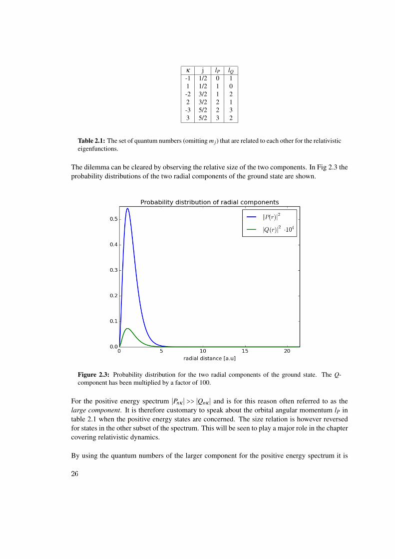
The dilemma can be cleared by observing the relative size of the two components. In Fig 2.3 theprobability distributions of the two radial components of the ground state are shown.
Figure 2.3: Probability distribution for the two radial components of the ground state. The Q-component has been multiplied by a factor of 100.
For the positive energy spectrum ∣Pnκ ∣ >> ∣Qnκ ∣ and is for this reason often referred to as thelarge component. It is therefore customary to speak about the orbital angular momentum lP intable 2.1 when the positive energy states are concerned. The size relation is however reversedfor states in the other subset of the spectrum. This will be seen to play a major role in the chaptercovering relativistic dynamics.
By using the quantum numbers of the larger component for the positive energy spectrum it is
26
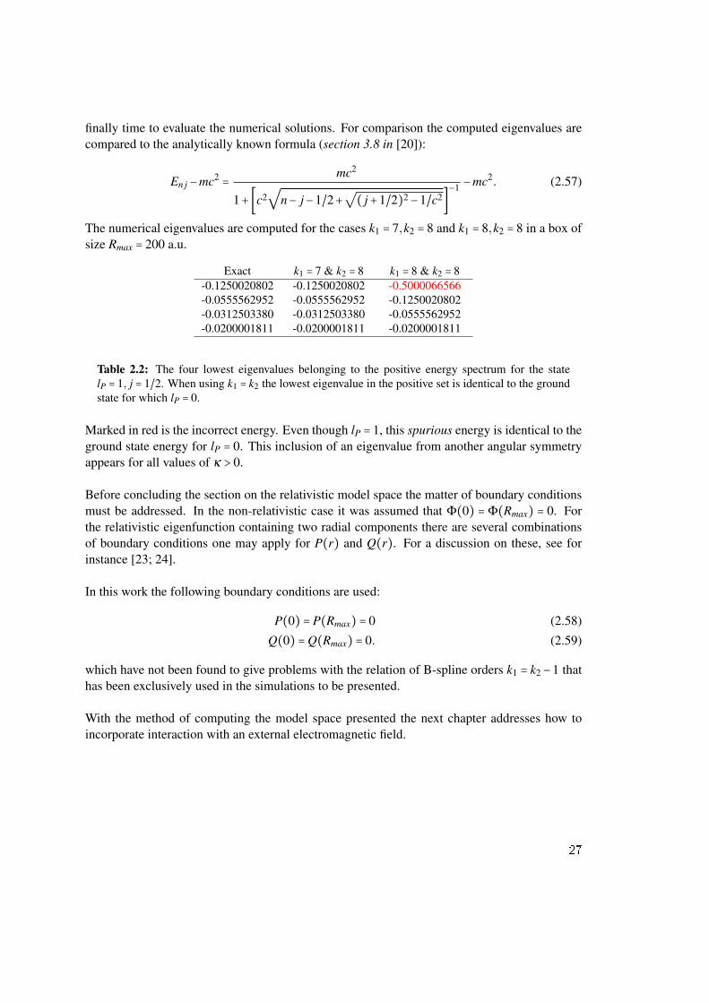
finally time to evaluate the numerical solutions. For comparison the computed eigenvalues arecompared to the analytically known formula (section 3.8 in [20]):
En j −mc2 = mc2
1+[c2√
n− j−1/2+√
( j+1/2)2−1/c2]−1 −mc2. (2.57)
The numerical eigenvalues are computed for the cases k1 = 7,k2 = 8 and k1 = 8,k2 = 8 in a box ofsize Rmax = 200 a.u.
Table 2.2: The four lowest eigenvalues belonging to the positive energy spectrum for the statelP = 1, j = 1/2. When using k1 = k2 the lowest eigenvalue in the positive set is identical to the groundstate for which lP = 0.
Marked in red is the incorrect energy. Even though lP = 1, this spurious energy is identical to theground state energy for lP = 0. This inclusion of an eigenvalue from another angular symmetryappears for all values of κ > 0.
Before concluding the section on the relativistic model space the matter of boundary conditionsmust be addressed. In the non-relativistic case it was assumed that Φ(0) = Φ(Rmax) = 0. Forthe relativistic eigenfunction containing two radial components there are several combinationsof boundary conditions one may apply for P(r) and Q(r). For a discussion on these, see forinstance [23; 24].
In this work the following boundary conditions are used:
P(0) = P(Rmax) = 0 (2.58)
Q(0) =Q(Rmax) = 0. (2.59)
which have not been found to give problems with the relation of B-spline orders k1 = k2−1 thathas been exclusively used in the simulations to be presented.
With the method of computing the model space presented the next chapter addresses how toincorporate interaction with an external electromagnetic field.
27
28
3. Interaction with an external field
I am no poet, but if you think for yourselves, as I proceed, the facts will form a poem in yourminds - Michael Faraday
The external electromagnetic field will be strong enough to be described by classical electro-magnetism. Therefore, this chapter is initiated with a recapitulation of Maxwell’s equations andthen followed by the computation of light-matter interaction.
3.1 Maxwell’s equations
The Maxwell equations describe any phenoma in classical electromagnetism. In free space theyread [25]:
∇∇∇⋅E = ρ
ε0(3.1)
∇∇∇×B = µ0J+ 1c2
∂E∂ t
(3.2)
∇∇∇⋅B = 0 (3.3)
∇∇∇×E = −∂B∂ t
(3.4)
where B and E are the magnetic and electric field, ρ and J the total charge and current density,ε0 and c the permittivity and speed of light in free space.
The set of four equations may be summarized in two equations coupled by a vector potential Aand a scalar field Φ. From eq. 3.3 one obtains:
∇∇∇⋅B = 0 → B =∇∇∇×A (3.5)
while eq. 3.5 inserted into eq. 3.4 gives:
∇∇∇×[E+ ∂A∂ t
] = 0 → E+ ∂A∂ t
= −∇Φ (3.6)
Similar substitutions and some more algebra give:
29
∇∇∇2Φ+ ∂
∂ t(∇∇∇⋅A) = − ρ
ε0(3.7)
∇2A− 1c2
∂2A
∂ t2 −∇∇∇(∇∇∇⋅A+ 1c2
∂Φ
∂ t) = −µ0J. (3.8)
There is a freedom in choosing the form of A and Φ as long as B and E, the objects of interest,remain unchanged. From eq. 3.5 and eq. 3.6 the conditions are:
A→A+∇∇∇χ (3.9)
Φ→Φ− ∂
∂ tχ (3.10)
for a scalar function χ. The freedom in scaling the fields A and Φ provides the means to trans-form them into a suitable form for a specific scenario. This type of transformation goes underthe name gauge transformation.
For the cases in this thesis there will be no sources present, i.e ρ = 0 and J = 0. In such a casethere exists a particularly useful gauge called the Coulomb gauge where ∇∇∇ ⋅A = 0. With nosources present the electric and magnetic fields in this gauge have the form:
E = −∂A∂ t
(3.11)
B =∇∇∇×A (3.12)
3.2 Interaction in general
The mathematical formulation of interaction is given by all operators1 in the Hamiltonian thatdepend on the field A (omitting arguments (r,t) for brevity). Incorporating the external field isdone by substituting p→ p+eA [17]:
note that eq. 3.13 assumes p ⋅A = A ⋅p which indeed is valid in Coulomb gauge. The inter-action within the model space is then evaluated by computing the matrix with elements:
HIHIHIab = ⟨Φa∣HI(t)∣Φb⟩ (3.15)
which may be done once the form of the pulse is known.
1In what follows, if it is clear from the context that an object is an operator the hat is left out.
30
3.3 Choosing a pulse
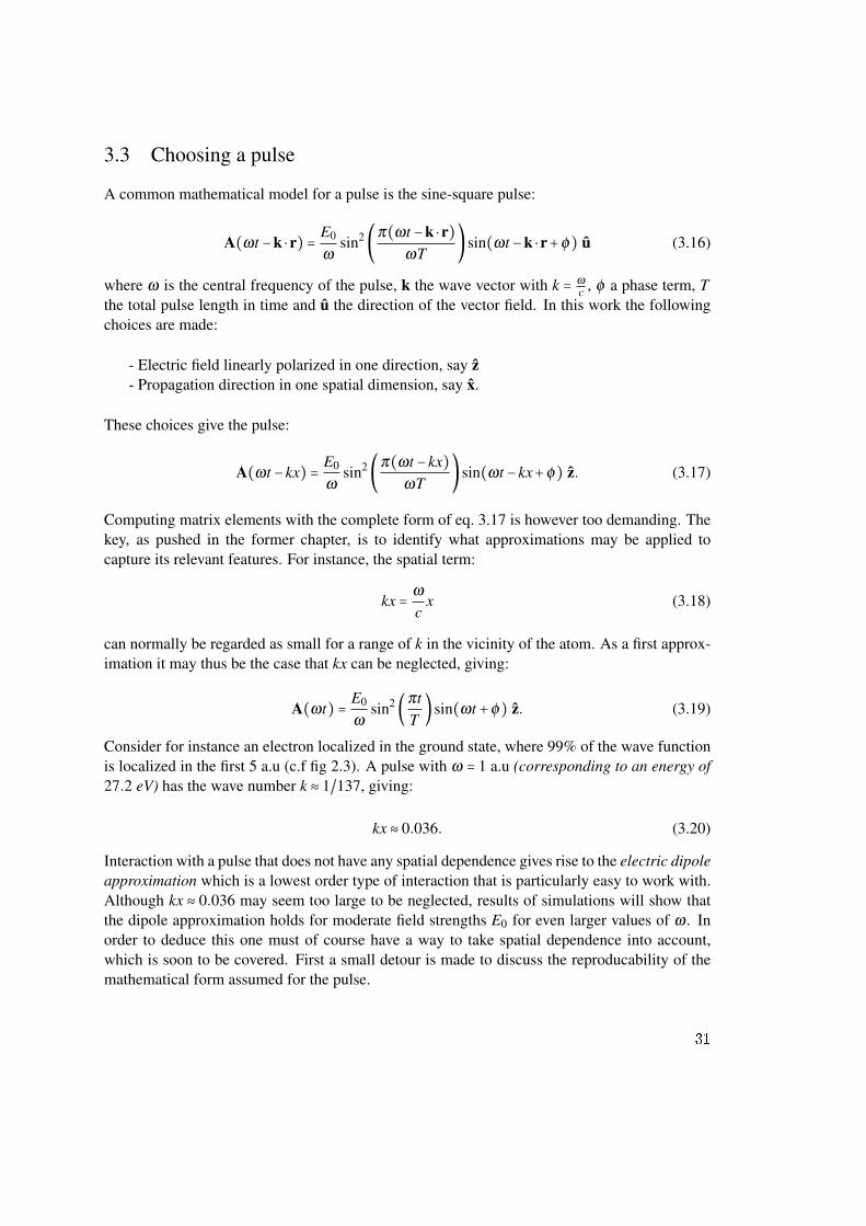
A common mathematical model for a pulse is the sine-square pulse:
A(ωt −k ⋅r) = E0
ωsin2(π(ωt −k ⋅r)
ωT)sin(ωt −k ⋅r+φ) u (3.16)
where ω is the central frequency of the pulse, k the wave vector with k = ω
c , φ a phase term, Tthe total pulse length in time and u the direction of the vector field. In this work the followingchoices are made:
- Electric field linearly polarized in one direction, say z- Propagation direction in one spatial dimension, say x.
These choices give the pulse:
A(ωt −kx) = E0
ωsin2(π(ωt −kx)
ωT)sin(ωt −kx+φ) z. (3.17)
Computing matrix elements with the complete form of eq. 3.17 is however too demanding. Thekey, as pushed in the former chapter, is to identify what approximations may be applied tocapture its relevant features. For instance, the spatial term:
kx = ω
cx (3.18)
can normally be regarded as small for a range of k in the vicinity of the atom. As a first approx-imation it may thus be the case that kx can be neglected, giving:
A(ωt) = E0
ωsin2(πt
T)sin(ωt +φ) z. (3.19)
Consider for instance an electron localized in the ground state, where 99% of the wave functionis localized in the first 5 a.u (c.f fig 2.3). A pulse with ω = 1 a.u (corresponding to an energy of27.2 eV) has the wave number k ≈ 1/137, giving:
kx ≈ 0.036. (3.20)
Interaction with a pulse that does not have any spatial dependence gives rise to the electric dipoleapproximation which is a lowest order type of interaction that is particularly easy to work with.Although kx ≈ 0.036 may seem too large to be neglected, results of simulations will show thatthe dipole approximation holds for moderate field strengths E0 for even larger values of ω . Inorder to deduce this one must of course have a way to take spatial dependence into account,which is soon to be covered. First a small detour is made to discuss the reproducability of themathematical form assumed for the pulse.
31
Pulse in the lab
Before doing anything more a pressing question should be addressed - how well can the pulseassumed be produced in the lab? In the figure below eq. 6 is plotted, for parameters given in thefigure, together with an experimentally produced pulse by ref [1]. The purpose of this figure isto show that the mathematical model given in the previous section is not too much of an ideal-ization.
Figure 3.1: Comparison of mathematical model (blue) with experimentally produced pulse (red).The bottom figure is adapted from [1].
32
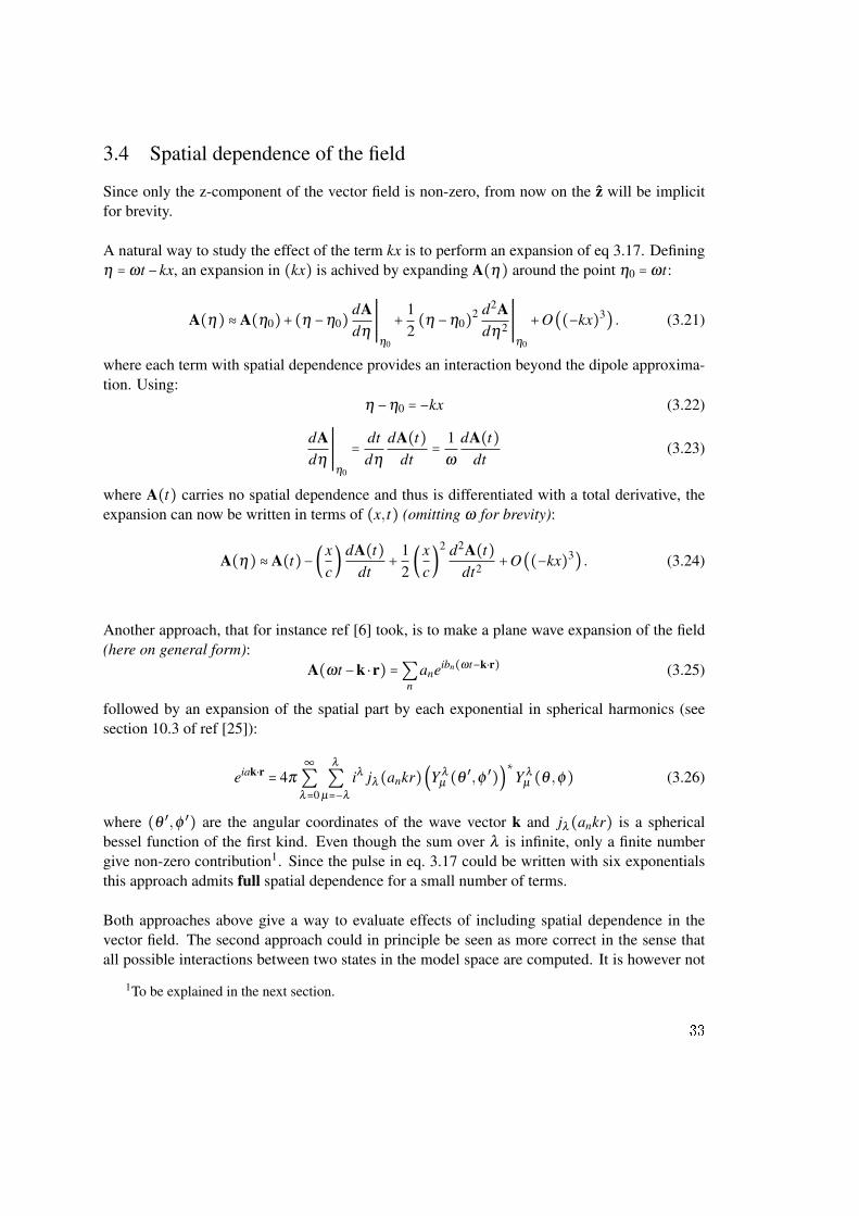
3.4 Spatial dependence of the field
Since only the z-component of the vector field is non-zero, from now on the z will be implicitfor brevity.
A natural way to study the effect of the term kx is to perform an expansion of eq 3.17. Definingη =ωt −kx, an expansion in (kx) is achived by expanding A(η) around the point η0 =ωt:
A(η) ≈A(η0)+(η −η0)dAdη
RRRRRRRRRRRη0
+ 12(η −η0)2 d2A
dη2
RRRRRRRRRRRη0
+O((−kx)3) . (3.21)
where each term with spatial dependence provides an interaction beyond the dipole approxima-tion. Using:
η −η0 = −kx (3.22)
dAdη
RRRRRRRRRRRη0
= dtdη
dA(t)dt
= 1ω
dA(t)dt
(3.23)
where A(t) carries no spatial dependence and thus is differentiated with a total derivative, theexpansion can now be written in terms of (x,t) (omitting ω for brevity):
A(η) ≈A(t)−(xc) dA(t)
dt+ 1
2(x
c)
2 d2A(t)dt2 +O((−kx)3) . (3.24)
Another approach, that for instance ref [6] took, is to make a plane wave expansion of the field(here on general form):
A(ωt −k ⋅r) =∑n
aneibn(ωt−k⋅r) (3.25)
followed by an expansion of the spatial part by each exponential in spherical harmonics (seesection 10.3 of ref [25]):
eiak⋅r = 4π
∞∑λ=0
λ
∑µ=−λ
iλ jλ (ankr)(Y λ
µ (θ′,φ ′))
∗Y λ
µ (θ ,φ) (3.26)
where (θ′,φ ′) are the angular coordinates of the wave vector k and jλ (ankr) is a spherical
bessel function of the first kind. Even though the sum over λ is infinite, only a finite numbergive non-zero contribution1. Since the pulse in eq. 3.17 could be written with six exponentialsthis approach admits full spatial dependence for a small number of terms.
Both approaches above give a way to evaluate effects of including spatial dependence in thevector field. The second approach could in principle be seen as more correct in the sense thatall possible interactions between two states in the model space are computed. It is however not
1To be explained in the next section.
33
practical1 and cannot be used to distinguish the importance of different types of higher orderinteractions. The reason for this is that all possible interactions between each individual pair ofstates are included.
This thesis is mainly based on the first method, in which a peculiar observation has been made:
TDDE does not seem to be stable for expansion 3.24 to first order in x.
Since there exist work published on first order corrections beyond the dipole approximation forTDSE, i.e [26], this observation was at first believed to be an artifact of incorrect source code.As it turns out, continuing the expansion leads to stability and agreement with the plane wavemethod. It also agrees with predictions by TDSE in a non-relativistic regime. These observa-tions give strong reasons to believe that this instability is not an artifact.
Now that the final forms of the vector field have been chosen the matrix elements can be com-puted. There are different ways to do this, for instance by using powerful tools from angularmomentum theory.
3.5 Spherical tensor operators and Wigner-Eckart theorem
When working in the spectral basis of an atomic system it is convenient to define a set of ba-sis operators which have known properties when acting upon angular momentum states. Byexpressing the interaction operator in this operator basis, complicated matrix elements may becomputed. The elements of this basis are called spherical tensor operators.
Let j = ( jx, jy, jz) be a general angular momentum vector and define j± = jx ± i jy. Consider anoperator with components of the form tk
q where q ∈ −k,−k+1, . . . ,k. If this operator satisfy:
[ jz,tkq] = qtk
q (3.27)
[ j±,tkq] = [k(k+1)−q(q±1)]1/2 tk
q±1 (3.28)
it is called a spherical tensor operator of rank k [27]. For such an operator the following powerfultheorem holds for matrix elements involving angular momentum (of any kind):
⟨nalama∣tkq ∣nblbmb⟩ = (-1)la−ma ( la k lb
-ma q mb)⟨nala∣∣tk∣∣nblb⟩ (3.29)
which is known as the Wigner-Eckart theorem. Note that the states are here characterized bytheir quantum numbers, which from now on is the default notation if not stated otherwise.
1Ref [6] discusses an additional physical argument that enforces even more computational load.
34
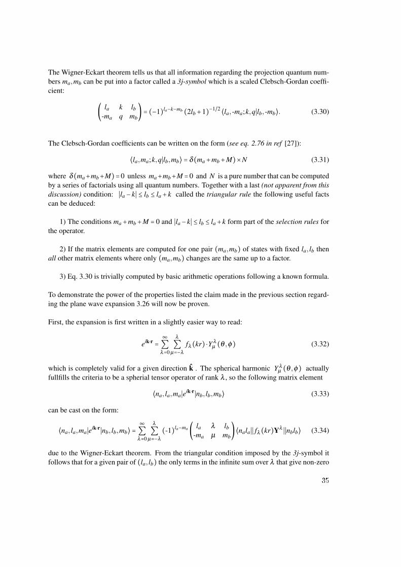
The Wigner-Eckart theorem tells us that all information regarding the projection quantum num-bers ma,mb can be put into a factor called a 3j-symbol which is a scaled Clebsch-Gordan coeffi-cient:
The Clebsch-Gordan coefficients can be written on the form (see eq. 2.76 in ref [27]):
⟨la,ma;k,q∣lb,mb⟩ = δ(ma+mb+M)×N (3.31)
where δ(ma+mb+M)= 0 unless ma+mb+M = 0 and N is a pure number that can be computedby a series of factorials using all quantum numbers. Together with a last (not apparent from thisdiscussion) condition: ∣la − k∣ ≤ lb ≤ la + k called the triangular rule the following useful factscan be deduced:
1) The conditions ma+mb+M = 0 and ∣la−k∣ ≤ lb ≤ la+k form part of the selection rules forthe operator.
2) If the matrix elements are computed for one pair (ma,mb) of states with fixed la, lb thenall other matrix elements where only (ma,mb) changes are the same up to a factor.
3) Eq. 3.30 is trivially computed by basic arithmetic operations following a known formula.
To demonstrate the power of the properties listed the claim made in the previous section regard-ing the plane wave expansion 3.26 will now be proven.
First, the expansion is first written in a slightly easier way to read:
eik⋅r =∞∑λ=0
λ
∑µ=−λ
fλ (kr) ⋅Y λ
µ (θ ,φ) (3.32)
which is completely valid for a given direction k . The spherical harmonic Y λµ (θ ,φ) actually
fullfills the criteria to be a spherial tensor operator of rank λ , so the following matrix element
⟨na, la,ma∣eik⋅r∣nb, lb,mb⟩ (3.33)
can be cast on the form:
⟨na, la,ma∣eik⋅r∣nb, lb,mb⟩ =∞∑λ=0
λ
∑µ=−λ
(-1)la−ma ( la λ lb-ma µ mb
)⟨nala∣∣ fλ (kr)Yλ ∣∣nblb⟩ (3.34)
due to the Wigner-Eckart theorem. From the triangular condition imposed by the 3j-symbol itfollows that for a given pair of (la, lb) the only terms in the infinite sum over λ that give non-zero
35
contributions are ∣la− lb∣ ≤ λ ≤ la+ lb.
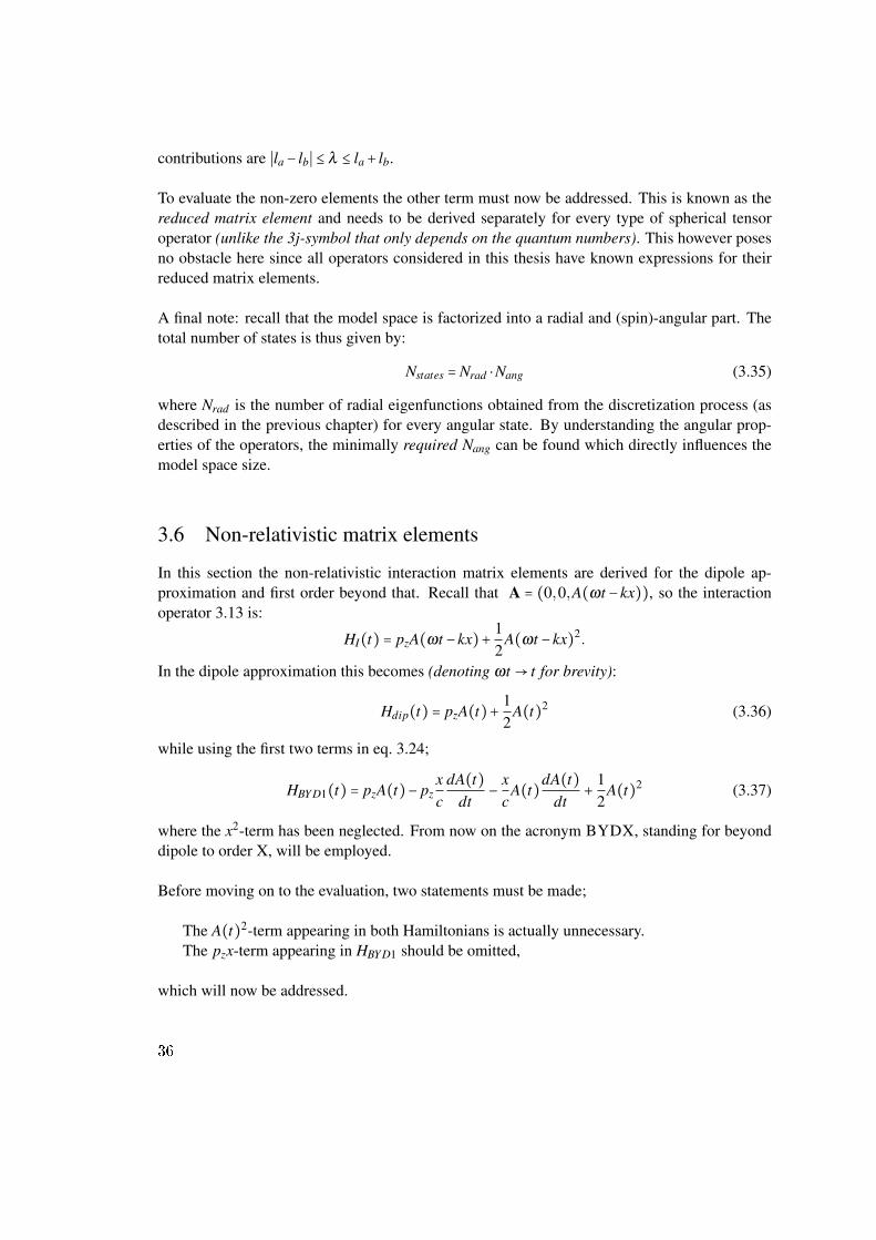
To evaluate the non-zero elements the other term must now be addressed. This is known as thereduced matrix element and needs to be derived separately for every type of spherical tensoroperator (unlike the 3j-symbol that only depends on the quantum numbers). This however posesno obstacle here since all operators considered in this thesis have known expressions for theirreduced matrix elements.
A final note: recall that the model space is factorized into a radial and (spin)-angular part. Thetotal number of states is thus given by:
Nstates =Nrad ⋅Nang (3.35)
where Nrad is the number of radial eigenfunctions obtained from the discretization process (asdescribed in the previous chapter) for every angular state. By understanding the angular prop-erties of the operators, the minimally required Nang can be found which directly influences themodel space size.
3.6 Non-relativistic matrix elements
In this section the non-relativistic interaction matrix elements are derived for the dipole ap-proximation and first order beyond that. Recall that A = (0,0,A(ωt −kx)), so the interactionoperator 3.13 is:
HI(t) = pzA(ωt −kx)+ 12
A(ωt −kx)2.
In the dipole approximation this becomes (denoting ωt → t for brevity):
Hdip(t) = pzA(t)+ 12
A(t)2 (3.36)
while using the first two terms in eq. 3.24;
HBY D1(t) = pzA(t)− pzxc
dA(t)dt
− xc
A(t)dA(t)dt
+ 12
A(t)2 (3.37)
where the x2-term has been neglected. From now on the acronym BYDX, standing for beyonddipole to order X, will be employed.
Before moving on to the evaluation, two statements must be made;
The A(t)2-term appearing in both Hamiltonians is actually unnecessary.The pzx-term appearing in HBY D1 should be omitted,
which will now be addressed.
36
The A(t)2 is unnecessary due to at least two reasons. One argument, perhaps not pointed out sooften, is that a purely time dependent operator is diagonal in a spatial basis. Hence it only shiftseigenvalues - it does not change the eigensolutions.
Another (often employed) argument is that A(t)2 can be removed by performing a gaugetransformation on the wave function itself, see e.g ref [28]. Although not of more relevance inthe present work, gauge transformations in light-matter interaction is a very important subjectthat deserves more than just a reference in passing. The interested reader is therefore referred toappendix for a short discussion on this subject.
The second statement is only motivated but not proven in detail here. In ref [28] the argument forremoving pzx from HBY D1 is based on a discussion of its physical significance. The authorspresent compelling reasons why the operator should be regarded as a second order correctionwhich therefore the current work also adopts.
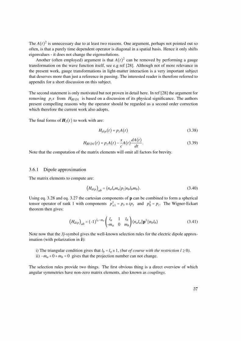
The final forms of HHHI(t) to work with are:
Hdip(t) = pzA(t) (3.38)
HBY D1(t) = pzA(t)− xc
A(t)dA(t)dt
. (3.39)
Note that the computation of the matrix elements will omit all factors for brevity.
3.6.1 Dipole approximation
The matrix elements to compute are:
(Hdip)ab = ⟨nalama∣pz∣nblbmb⟩. (3.40)
Using eq. 3.28 and eq. 3.27 the cartesian components of p can be combined to form a sphericaltensor operator of rank 1 with components p1
±1 = px ± ipy and p10 = pz. The Wigner-Eckart
theorem then gives:
(Hdip)ab = (-1)la−ma ( la 1 lb-ma 0 mb
)⟨nala∣∣p1∣∣nblb⟩ (3.41)
Note now that the 3j-symbol gives the well-known selection rules for the electric dipole approx-imation (with polarization in z):
i) The triangular condition gives that lb = la±1, (but of course with the restriction l ≥ 0).ii) −ma+0+mb = 0 gives that the projection number can not change.
The selection rules provide two things. The first obvious thing is a direct overview of whichangular symmetries have non-zero matrix elements, also known as couplings.
37
The second thing is the required Nang for a given maximum angular momentum lmax considered.While there are 2l+1 different values of ml for every value of l, the pz-operator can only connectstates with the same ml . If the initial state prior to interaction has a fixed value of ml , i.e ml = 0,the required angular model space has:
Nang = lmax+1 (3.42)
number of states. It is of course not incorrect to include states with different values of ml as wellbut it is in this case just dead weight.
What remains now is to complete the matrix element is to compute the reduced matrix element.The explicit form of this for p1 can be found in ref [29]. As there is no aspect from its appear-ance that is needed to follow the development of this thesis, it is not addressed further here.
3.6.2 Beyond the dipole approximation
The matrix elements to compute here are:
⟨nalama∣pz∣nblbmb⟩ (3.43)
⟨nalama∣x∣nblbmb⟩. (3.44)
The x-operator can be rewritten in spherical harmonics of rank 1:
x = r ⋅√
2π
3(Y 1
-1−Y 11 ) (3.45)
and applying the Wigner-Eckart theorem to this gives:
⟨nalama∣x∣nblbmb⟩ =√
2π
3⋅(-1)la−ma (( la 1 lb
-ma -1 mb)−( la 1 lb
-ma 1 mb))⟨nala∣∣rY1∣∣nblb⟩. (3.46)
The conditions from the 3j-symbol give:i) The triangular condition gives lb = la±1.ii) −ma±1+mb = 0 gives that the projection number changes; mb =ma±1.
This operator connects states with different values of ml and thus forces the model space to grow.Given a specific initial state, say the (angular) ground state ∣l = 0,ml = 0⟩ the following states (upto l=2) can be reached:
∣l = 1,ml = ±1⟩, ∣l = 2,ml = ±2⟩, ∣l = 2,ml = 0⟩.
If the interaction was only given by the x-operator some states could be omitted; for instance∣l = 1,ml = 0⟩, ∣l = 2,ml =±1⟩. The interaction however also includes the pz-operator that connects
38
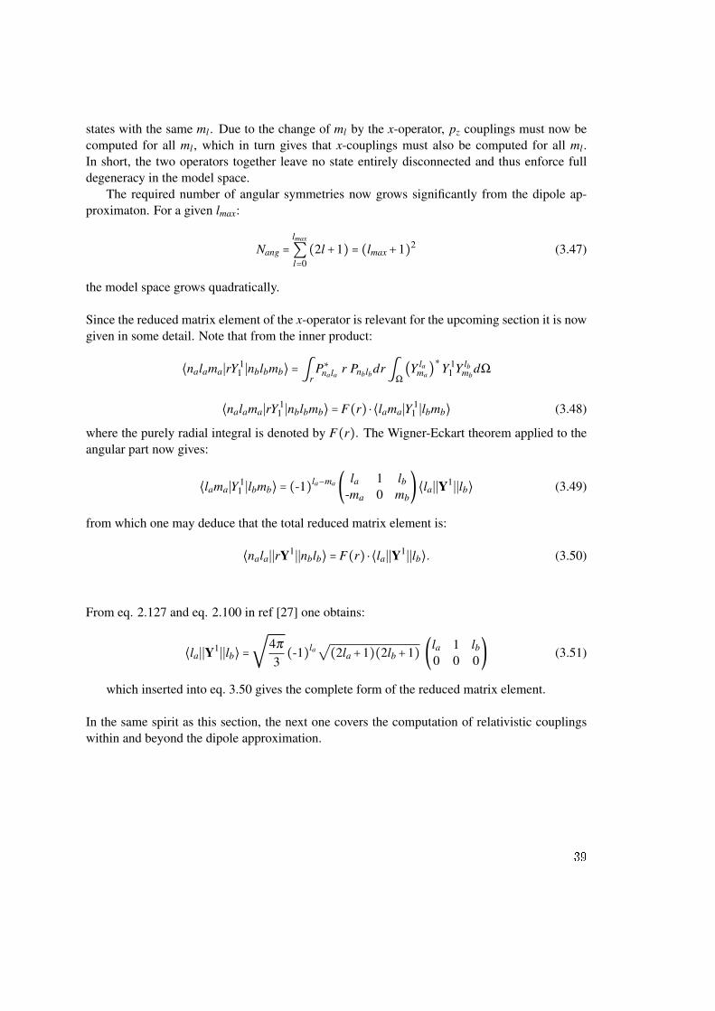
states with the same ml . Due to the change of ml by the x-operator, pz couplings must now becomputed for all ml , which in turn gives that x-couplings must also be computed for all ml .In short, the two operators together leave no state entirely disconnected and thus enforce fulldegeneracy in the model space.
The required number of angular symmetries now grows significantly from the dipole ap-proximaton. For a given lmax:
Nang =lmax
∑l=0
(2l+1) = (lmax+1)2 (3.47)
the model space grows quadratically.
Since the reduced matrix element of the x-operator is relevant for the upcoming section it is nowgiven in some detail. Note that from the inner product:
⟨nalama∣rY 11 ∣nblbmb⟩ = ∫
rP∗nala r Pnblbdr∫
Ω
(Y lama
)∗Y 11 Y lb
mbdΩ
⟨nalama∣rY 11 ∣nblbmb⟩ = F(r) ⋅ ⟨lama∣Y 1
1 ∣lbmb⟩ (3.48)
where the purely radial integral is denoted by F(r). The Wigner-Eckart theorem applied to theangular part now gives:
⟨lama∣Y 11 ∣lbmb⟩ = (-1)la−ma ( la 1 lb
-ma 0 mb)⟨la∣∣Y1∣∣lb⟩ (3.49)
from which one may deduce that the total reduced matrix element is:
⟨nala∣∣rY1∣∣nblb⟩ = F(r) ⋅ ⟨la∣∣Y1∣∣lb⟩. (3.50)
From eq. 2.127 and eq. 2.100 in ref [27] one obtains:
⟨la∣∣Y1∣∣lb⟩ =√
4π
3(-1)la
√(2la+1)(2lb+1) (la 1 lb
0 0 0) (3.51)
which inserted into eq. 3.50 gives the complete form of the reduced matrix element.
In the same spirit as this section, the next one covers the computation of relativistic couplingswithin and beyond the dipole approximation.
39
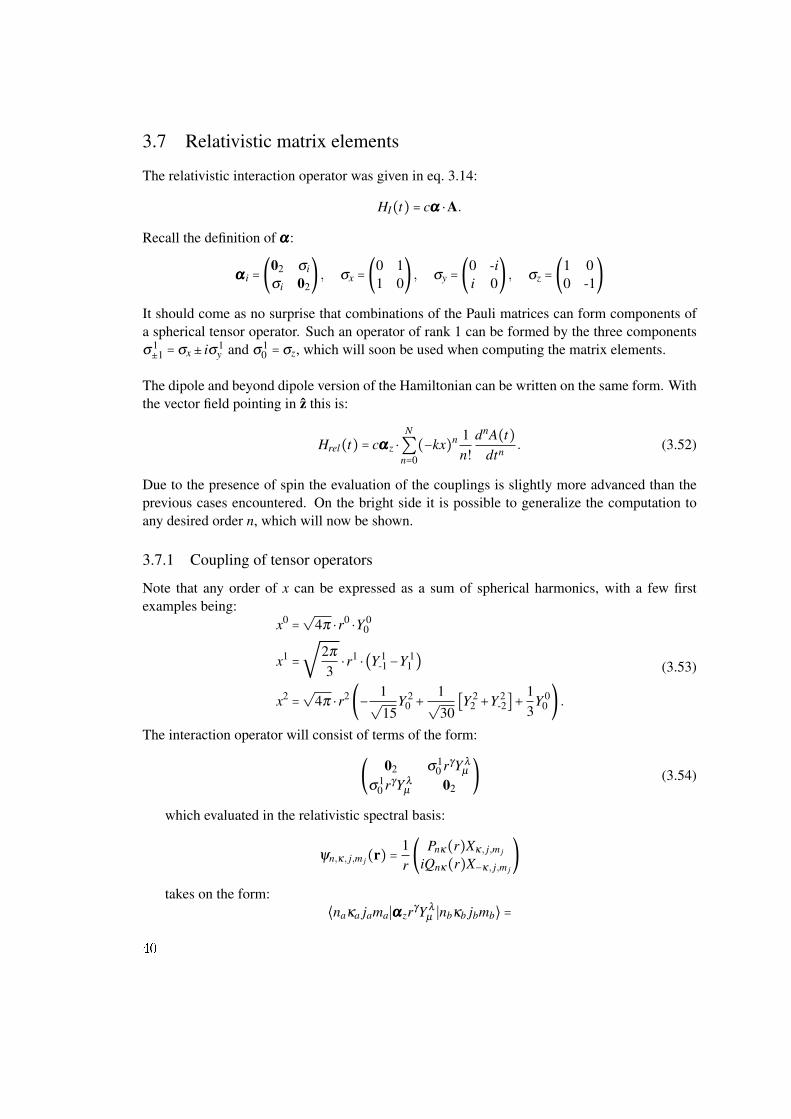
3.7 Relativistic matrix elements
The relativistic interaction operator was given in eq. 3.14:
HI(t) = cααα ⋅A.
Recall the definition of ααα:
ααα i = (02 σi
σi 02) , σx = (0 1
1 0) , σy = (0 -i
i 0) , σz = (1 0
0 -1)
It should come as no surprise that combinations of the Pauli matrices can form components ofa spherical tensor operator. Such an operator of rank 1 can be formed by the three componentsσ
1±1 = σx± iσ1
y and σ10 = σz, which will soon be used when computing the matrix elements.
The dipole and beyond dipole version of the Hamiltonian can be written on the same form. Withthe vector field pointing in z this is:
Hrel(t) = cαααz ⋅N
∑n=0
(−kx)n 1n!
dnA(t)dtn . (3.52)
Due to the presence of spin the evaluation of the couplings is slightly more advanced than theprevious cases encountered. On the bright side it is possible to generalize the computation toany desired order n, which will now be shown.
3.7.1 Coupling of tensor operators
Note that any order of x can be expressed as a sum of spherical harmonics, with a few firstexamples being:
x0 =√
4π ⋅ r0 ⋅Y 00
x1 =√
2π
3⋅ r1 ⋅(Y 1
-1−Y 11 )
x2 =√
4π ⋅ r2(− 1√15
Y 20 +
1√30
[Y 22 +Y 2
-2]+13
Y 00 ) .
(3.53)
The interaction operator will consist of terms of the form:
( 02 σ10 rγY λ
µ
σ10 rγY λ
µ 02) (3.54)
which evaluated in the relativistic spectral basis:
ψn,κ, j,m j(r) = 1r( Pnκ(r)Xκ, j,m j
iQnκ(r)X−κ, j,m j
)
takes on the form:⟨naκa jama∣αααzrγY λ
µ ∣nbκb jbmb⟩ =
40
i∫r[P∗naκa
(r)rγQnbκb(r)⟨κa jama∣σ10Y λ
µ ∣-κb jbmb⟩− (3.55)
Q∗naκa
(r)rγPnbκb(r)⟨-κa jama∣σ10Y λ
µ ∣κb jbmb⟩dr].
While the radial integrals are of the same form as before, the spin-angular part is different.This time the interaction operator is a tensor product with one tensor (σ1
0 ) acting in spin-spacewhile the other term acts in the orbital angular momentum space. While such a point of view isperfectly valid another useful approach exists: to couple the operators together to form a singleoperator acting in the combined spin-angular Hilbert space1:
σ10Y λ
µ =λ+1
∑K=∣λ−1∣
⟨10;λ µ ∣KQ⟩σσσ1Yλ
K
Q, Q = −µ
With this choice the spin-angular part may be computed as2:
⟨κ jm∣σ10Y λ
µ ∣κ jm⟩ = ⟨κ jm∣λ+1
∑K=∣λ−1∣
⟨10;λ µ ∣KQ⟩σσσ1Yλ
K
Q∣κ jm⟩
⟨κ jm∣σ10Y λ
µ ∣κ jm⟩ =λ+1
∑K=∣λ−1∣
⟨10;λ µ ∣KQ⟩⟨κ jm∣σσσ1Yλ
K
Q∣κ jm⟩
using eq. 3.30:
⟨κ jm∣σ10Y λ
µ ∣κ jm⟩ =λ+1
∑K=∣λ−1∣
(-1)λ−1−Q√2K+1(1 λ K
0 µ −µ)⟨κ jm∣σσσ
1YλK
Q∣κ jm⟩ (3.56)
The Wigner-Eckart theorem can be applied to the matrix element of the combined operatorσσσ
1YλKQ:
⟨κ jm∣σσσ1Yλ
K
Q∣κ jm⟩ = (-1) j−m( j K j
−m Q m)⟨ j∣∣σσσ
1YλK∣∣ j⟩ (3.57)
Lastly, the reduced matrix element of the combined operator is (see eq. 4.21 in ref [27]):
⟨ j∣∣σσσ1Yλ
K∣∣ j⟩ =
√(2 j+1)(2K+1)(2 j+1)⟨s∣∣σσσ1∣∣s⟩⟨l∣∣Yλ ∣∣l⟩
⎧⎪⎪⎪⎨⎪⎪⎪⎩
l l 1s s λ
j J K
⎫⎪⎪⎪⎬⎪⎪⎪⎭(3.58)
where the last expression is a 9 j-symbol, which can be written as the product of 3 j-symbols (seeeq. 3.71 in ref [27]). The term 3.55 can now be computed by starting with eq. 3.58 and traceback through the numbered equations.
1See for instance eq. 2.95 in ref [27] which is the inverted relation.2To tidy up, the indices are temporarily replaced.
41
It is perhaps not trivial to digest what just happened. However, the overwhelming power of theapproach should be clear: these steps are programmed just once. Incorportating couplings toany spatial order, say n, only requires the extra work of expressing xn in spherical harmonics -no additional source code need to be developed.
On a final note, due to the presence of spin, the number of angular states in the relativistic frame-work is twice the size of the non-relativistic angular basis. Together with the two radial com-ponents the relativistic model space is four times larger than the correspnding non-relativisticspace.
42
4. Dynamics
Premature optimization is the root of all evil - Donald Knuth
This chapter lays the foundation for computing the dynamics using the couplings from the pre-vious chapter. One final numerical technique to alter the model space called complex scaling isintroduced. In order to prepare for higher order dynamics with model spaces containing up to106 states, several successful (and some unsuccessful) steps of optimization have been made.
4.1 Time evolution operator
The equations of motion may be put on another form than have been seen thus far:
∣Ψ(t1)⟩ = U(t0,t1)∣Ψ(t0)⟩ (4.1)
where U(t0,t1) is known as the time evolution operator. For a time dependent Hamiltonian thatcommutes with itself at different times it is:
U(t0,t1) = e−i∫t1
t0H(t′)dt′
which can be found in for instance ref [17]. Given a small enough time separation ∆t = t1−t0→ 0this may be approximated as:
U(t0,t1) ≈ e−iH(t0+∆t/2)⋅∆t (4.2)
For the attentive, this approximation is just the mean-value theorem. Propagation now amountsto understanding how to compute the action of the matrix exponential on the state ∣Ψ(t0)⟩.
4.2 Expansion in field dressed eigenstates
Recall that the spectral basis Φ(t) of the Hamiltonian, at any time, is complete. It is thereforepossible to express the unity operator as:
1 =∑n∣Φn(t)⟩⟨Φn(t)∣. (4.3)
Inserting the last two equations into eq. 4.1 one obtains:
∣Ψ(t0+∆t)⟩ ≈ e−iH(t0+∆t/2)⋅∆t 1∣Ψ(t0)⟩
43
∣Ψ(t0+∆t)⟩ ≈∑n
e−iEn(t0+∆t/2)⋅∆t ∣Φn(t +∆t/2)⟩⟨Φn(t)∣Ψ(t0+∆t/2)⟩
where the exponential operator acted on the eigenstates of H(t0+∆t/2). The way to achievethis in a numerical basis is to compute the time dependent Hamiltonian:
H(t) =H0+HI(t) (4.4)
where the interaction matrix elements are computed by multiplying each operator with thecorresponding time factor, i.e:
(HI(t))ab = A(t) ⋅ ⟨Φa∣σz∣Φb⟩−ω
cdAdt
⋅ ⟨Φa∣σzx∣Φb⟩ (4.5)
for the first order relativistic BYD Hamiltonian. Once the Hamiltonian is built the eigenvaluesand eigenvectors of this matrix are obtained from diagonalizing the matrix.
Now an extremely important question arises - what about the negative energy states?
4.2.1 Negative energy states
Recall that the relativistic spectrum contains negative energy states. Dirac’s interpretation ofthese states were to regard them as naturally occupied. If they were reachable, then any positiveenergy eigenstate would decay into the negative spectrum. Now the question arises: unless thereis real pair-production, can these states be left out of the basis set? That is; from the spectralbasis of the time independent Dirac Hamiltonian, is it valid to remove all eigenstates belongingto the negative energy spectrum? In general, the answer is no (see ref [6; 7]), which at first seemsto contradict Dirac’s original hypothesis.
However, the conclusion reached in ref [6] is that the hypothesis applies to the time depen-dent basis, since what constitutes a negative energy state changes with the field. The omissionof the "true" states is then achieved by only projecting the state ∣Ψ(t0)⟩ onto the time dependentpositive energy states P:
∣Ψ(t0+∆t)⟩ ≈∑n∈P
e−iEn(t0+∆t/2)⋅∆t ∣Φn(t +∆t/2)⟩⟨Φn(t)∣Ψ(t0+∆t/2)⟩
.The conclusion above works nicely with the technique employed to compute a small and effi-cient radial model space: complex scaling.
4.3 Limiting the box size with complex scaling
One condition to put on a model space is that it should not introduce artificial effects. If themodel space is not big enough unreliable results are to be expected:
44
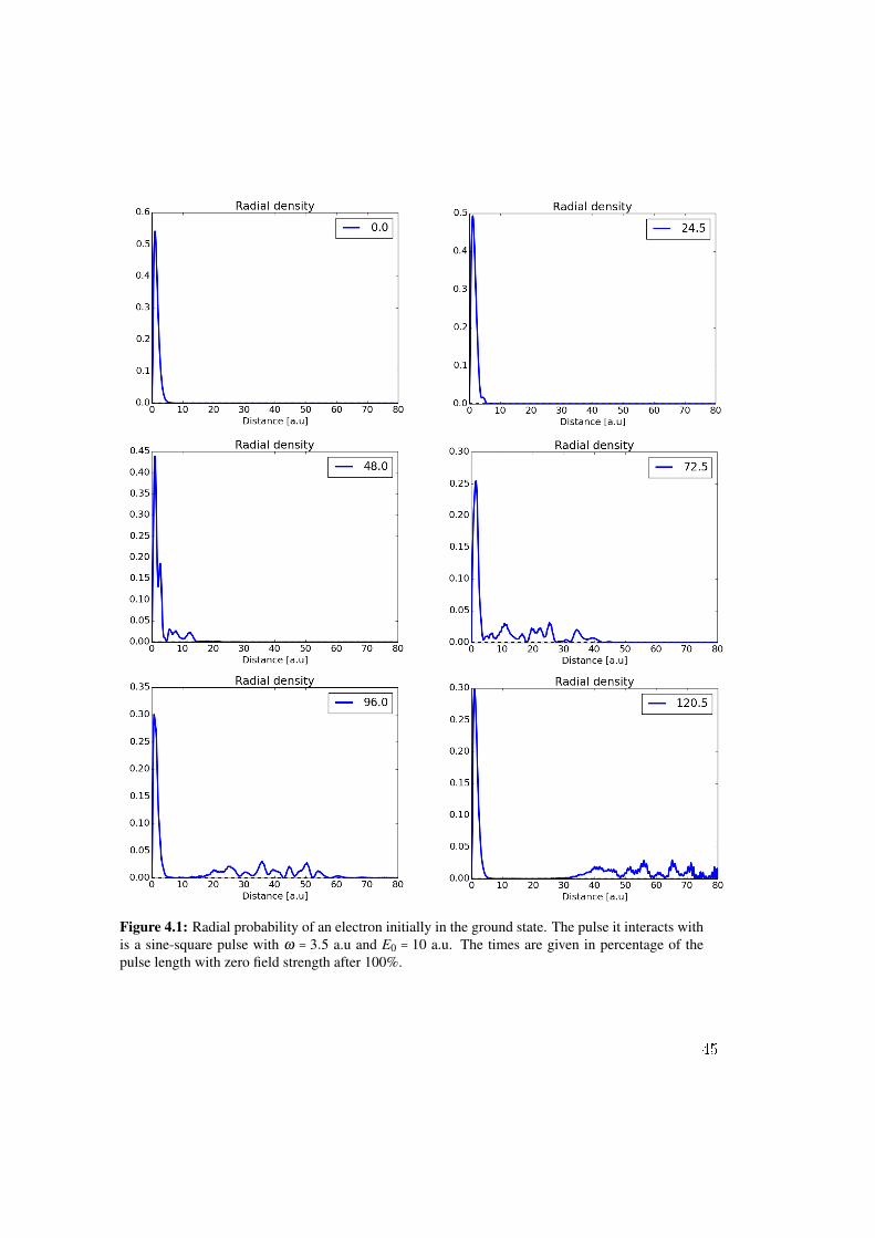
Figure 4.1: Radial probability of an electron initially in the ground state. The pulse it interacts withis a sine-square pulse with ω = 3.5 a.u and E0 = 10 a.u. The times are given in percentage of thepulse length with zero field strength after 100%.
45
In fig. 4.1 it is seen that as the wave function moves outwards it hits the box end and reflectsback. At the field strengths to be considered (E0 ∼ 130 a.u) it is not feasible to just make the boxlarger, which is seen in Fig. 4.2 below. Here the box is increased to Rmax = 300 a.u while the fieldstrength is E0 = 60 a.u. While the majority of the wave function is localized within 50 a.u fromthe nucleus small ripples of probability continuously shoot out towards the box end. Eventuallythat miniscule part hits the box end and propagates back to interfere with the rest of the wavefunction.
Figure 4.2: Radial probability of an electron initially in the ground state. Here E0 = 60 a.u. whilethe other pulse parameters are the same as in Fig. 4.1.
One way to overcome this obstacle is to use complex scaling. In this method the radial coordinateis rotated with an angle θ into the complex plane; either from r = 0, called uniform complexscaling:
r→ eiθ r (4.6)
46
or starting from some value r0:
r→ r0+(r− r0)eiθ r, r > r0 (4.7)
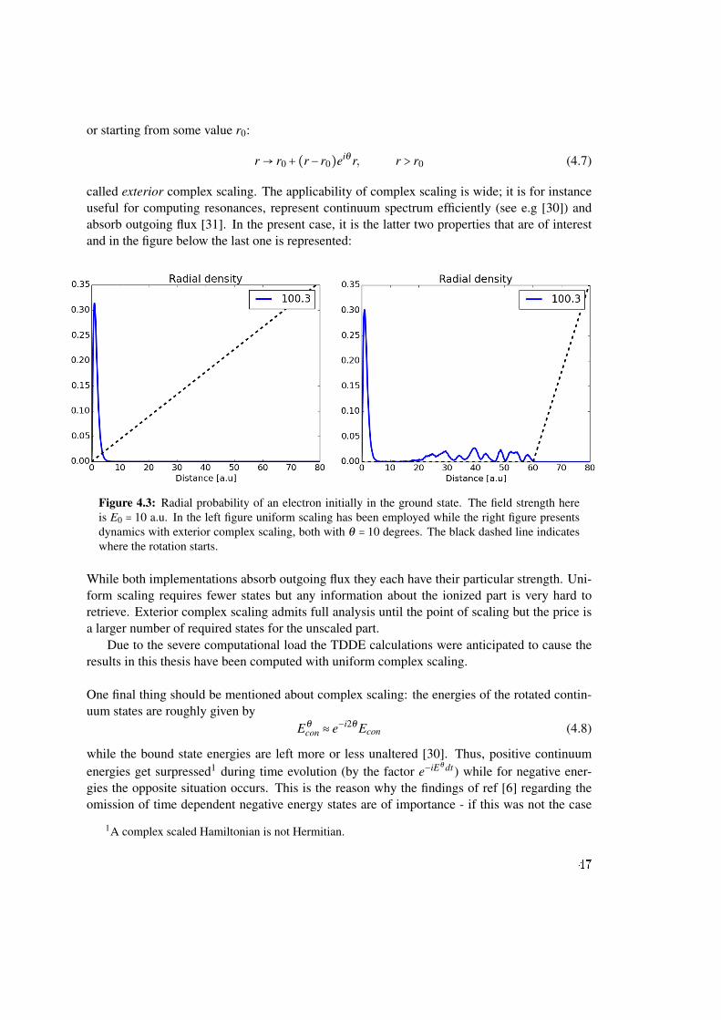
called exterior complex scaling. The applicability of complex scaling is wide; it is for instanceuseful for computing resonances, represent continuum spectrum efficiently (see e.g [30]) andabsorb outgoing flux [31]. In the present case, it is the latter two properties that are of interestand in the figure below the last one is represented:
Figure 4.3: Radial probability of an electron initially in the ground state. The field strength hereis E0 = 10 a.u. In the left figure uniform scaling has been employed while the right figure presentsdynamics with exterior complex scaling, both with θ = 10 degrees. The black dashed line indicateswhere the rotation starts.
While both implementations absorb outgoing flux they each have their particular strength. Uni-form scaling requires fewer states but any information about the ionized part is very hard toretrieve. Exterior complex scaling admits full analysis until the point of scaling but the price isa larger number of required states for the unscaled part.
Due to the severe computational load the TDDE calculations were anticipated to cause theresults in this thesis have been computed with uniform complex scaling.
One final thing should be mentioned about complex scaling: the energies of the rotated contin-uum states are roughly given by
Eθ
con ≈ e−i2θ Econ (4.8)
while the bound state energies are left more or less unaltered [30]. Thus, positive continuumenergies get surpressed1 during time evolution (by the factor e−iEθ dt) while for negative ener-gies the opposite situation occurs. This is the reason why the findings of ref [6] regarding theomission of time dependent negative energy states are of importance - if this was not the case
1A complex scaled Hamiltonian is not Hermitian.
47
complex scaling would probably only cause problems when applied to TDDE.
4.4 Krylov subspace method
With uniform complex scaling, the radial basis size can be kept small. Despite this, a full diag-onalization is for practical purposes not feasible as the number of angular symmetries requriedwill be very large. In such a case a Krylov subspace technique might be useful.
The idea, made readily accessible in ref [32] together with ref [33], is to approximate the actionof the time evolution operator:
eH x ≈ pm−1(H)x (4.9)
where H = −iH(t +∆t/2)∆t and pm−1(H) is a polynomial in H of order m−1. This polynomialbelongs to the space spanned by:
Km = x,Hx, . . . ,Hm−1x (4.10)
where Km is called a Krylov space of order m. Note that most of the symbols and indices arekept similar to the notation in [32; 33] for the benefit of the reader.
Following the Arnoldi algorithm outlined in sec.2.1 of ref [32], an orthonormal basis Vm ofthe Krylov space can be constructed. In [33] the following approximation is made:
eH ≈VmeUmV Tm (4.11)
where Um =V Tm HVm. The geometrical interpretation of this is that the matrix exponential in the
Hilbert space, eH , is projected onto the Krylov subspace spanned by the basis Vm. Given a shortenough time step ∆t, the dimension of this space m can be made very small. For the strongestfields considered in this thesis some typical values are ∆t ≈ 0.02 ∼ 0.04 with Krylov subspacesof order m ∼ 15. The convergence with respect to m can be monitored by computing one of theerror estimates given in ref [32].
Note that the matrix exponential in Krylov space can be evaluated in complete analogy asthe full diagonalization:
eH ≈VmeUm 1mV Tm =Vm [
m
∑n=1
eEn ∣φn⟩⟨φn∣]V Tm (4.12)
with the exception that this time the diagonalization is made in the 15×15 space which isdone in an instance. Now the time consuming part is dominated by matrix-vector products.These can however be siginificantly optimized which is the subject up next.
4.4.1 Optimization
Consider the basis of the relativistic model space ordered in increasing (l, j,m j) (for the largecomponent), i.e ∣0, 1
2 ,-12⟩, ∣0, 1
2 ,12⟩, ∣1, 1
2 ,-12⟩, ∣1,
12 ,
12⟩, ∣1, 3
2 ,-32⟩, ∣1, 3
2 ,-12⟩ and so on up to l = 6.
The four first spatial operators then take on the following appearance:
48
Figure 4.4: Relativistiv couplings matrices. Each coloured block denotes a coupling of thecorrsponding operator between two states. In general, the operator contains a lof of zero entriesand as such is said to be sparse.
Each block is an (Nrad ×Nrad) submatrix, typically with Nrad ∼ 100. While the coloured blocksrepresent interaction the rest are just zeros that fill up system memory - but the tragedy does notnecessarily stop there. In case these matrices are multiplied with vectors using normal routines(non-sparse) a lot of zero-multiplication take place.
By only using the non-zero elements significant memory and computational time is freedup. It is also easily parallelized both on shared memory machines as well as distributed systemswhich can give a new level of performance to the program. The optimization does however notstop just quite yet.
Recall the essence of the Wigner-Eckart theorem: all information regarding projection numberscan be factored out of the matrix element. This means that a lot of the blocks in the previousfigure should only differ by a scalar.
49
Figure 4.5: A comparison between the full BYD3 angular couplings with the reduced matrix ele-ments not duplicated. The left figure can be reproduced from the right by just multiplication of thecorrect angular factor.
The final form of the propagation builds a Krylov subspace for many small time steps. At eachstep, products of the form H(t)∣Ψ⟩ are computed by applying the angular and radial factorsseparately to ∣Ψ⟩ to minimize the total number of operations. As a comparison, consider theFig. 4.6
50
Figure 4.6: Probability to find the electron in the ground state as a function of time. The pulse herehas a total time of T = 30π a.u, E0 = 40.0 a.u and ω = 3.5 a.u. The dots are the results from dynamicswith full coupling matrices while the red solid line is an optimized Krylov implementation.
To demonstrate the increased performance a table showing the memory and time consumptionof the two approaches is given below.
Time [s] Time step [a.u] MemoryFull 3 ⋅106 0.25 2.0 GB
Optimized Krylov 3 ⋅102 0.02 40 kB
Table 4.1: Comparing figures for full and Krylov implementation. The model space here consistsof 2×20 B-splines per angular symmetry, with 128 such included. (lmax = 7).
The same Krylov implementation is adopted for the non-relativistic simulations. In the nextchapter results of simulations are shown.
51
52
5. Results
Everything uptil now has been in preparation to solve the equations of motion. By doing so oneshould in principle be able to obtain any desired information about the system. However, due tothe use of uniform complex scaling some observables are for practical purposes out of reach -for instance the angular distribution of the electron.
One observable that still is computable is the total photoionization yield, Pion, which is theprobability that the electron due to the interaction leaves the system.
Relativistic effects are expected when the classical quiver velocity of the electron vq ∼ E0ω
, reachesa substantial fraction of the speed of light [28] [2]1. In this chapter results are presented for dy-namics up to vq ≈ 0.23c (E0 = 110 a.u) to explicitly compare the predictions by TDSE and TDDE.
5.1 Model space and pulse parameters
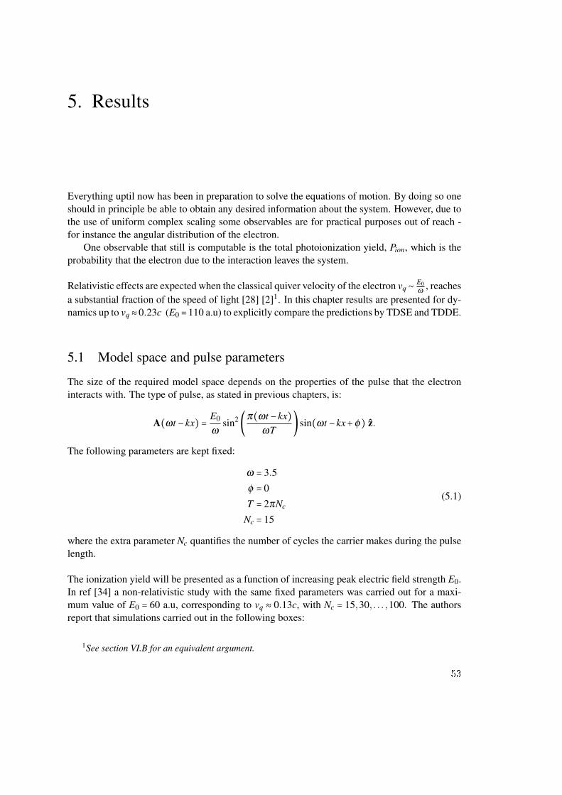
The size of the required model space depends on the properties of the pulse that the electroninteracts with. The type of pulse, as stated in previous chapters, is:
A(ωt −kx) = E0
ωsin2(π(ωt −kx)
ωT)sin(ωt −kx+φ) z.
The following parameters are kept fixed:
ω = 3.5
φ = 0
T = 2πNc
Nc = 15
(5.1)
where the extra parameter Nc quantifies the number of cycles the carrier makes during the pulselength.
The ionization yield will be presented as a function of increasing peak electric field strength E0.In ref [34] a non-relativistic study with the same fixed parameters was carried out for a maxi-mum value of E0 = 60 a.u, corresponding to vq ≈ 0.13c, with Nc = 15,30, . . . ,100. The authorsreport that simulations carried out in the following boxes:
1See section VI.B for an equivalent argument.
53
i) A very large box of Rmax = 800 a.uii) A smaller box of Rmax = 40 a.u with an absorbing potential for outgoing flux
give the same values for the ionization yield. Given the much shorter propagation time usedhere (15 cycles, compared to their 100 cycles) the smaller box should be sufficient for the fieldstrengths considered here (E0 ≤ 110 a.u). Thus, computations are carried out in the followingbox:
Rmax 40.0 a.udr 0.34 a.uθ 2.5
B-spline order 7 (Pnonrel ,Prel), 8 (Qrel)Number of B-splines 121 (Pnonrel ,Prel), 122 (Qrel)
Table 5.1: Grid parameters for model box. The same equidistant knot sequence is used for TDSEand TDDE computation. Note that the relativistic computations require twice as many radial statesdue to having two components. Since the angular basis is twice as large due to spin, the relativisticbasis is four times larger than the non-relativistic basis for the same box and lmax.
A sufficient size of the angular model space is monitored by increasing the maximum orbital an-gular momentum lmax (including all states with lower l and full degeneracy) until the dynamicshave converged. Once the final model space is acquired Pion can be computed by solving TDSEand TDDE in the various spatial approximations of the pulse that were discussed in chapter 3.Pion is in this work computed as the sum of population in the bound numerical box states.
Before moving on to discuss the results of the dynamics a reminder of the time dependent Hamil-tonians is in order:
Hnrel(t) =H0+ pzA(t)− xc
A(t)dA(t)dt
.
Hrel(t) =HD0 +cαz ⋅A(t)+cαz ⋅N
∑n=1
(−kx)n 1n!
dnA(t)dtn .
(5.2)
where the value of N will be discussed in subsequent sections. Before that, the next sectionpresents Pion predicted by the dipole approximation, where any dependence on x is neglected.
5.2 Dipole interaction
Consider first the interaction without a spatial dependence of the pulse. Fig. 5.1 shows Pion for athe box described in tab. 5.1 with increasing values of lmax.
54
Figure 5.1: Ionization probability for hydrogen as a function of the peak electric field strength. Thevertical line denotes the value of E0 for which vq ≈ 0.1c. Note the convergence with increasing lmaxtowards the black solid line which is globally converged to 10−5 (see figure below).
Figure 5.2: Global convergence test of the dipole approximation. The difference between lmax = 40and lmax = 15,20,30 are shown. The residual of lmax = 30 is of the order 10−5 which is in the currentcontext will be accepted as converged. Note the second vertical line here indicating another 10%-increment of speed of light. 55
The discontinuous jumps of Pion(E0) for lower values of lmax in fig. 5.1 are typical for an incom-plete basis, that is, a basis that does not provide enough channels for the dynamics. This is alsothe reason why the jumps disappear when more channels (larger lmax) are included.
Before leaving the section on dipole approximation, converged calculations for TDSE andTDDE are compared:
Figure 5.3: Comparison of TDSE and TDDE calculation (lmax = 40) within the dipole approxima-tion. At vq ≈ 0.15c, the non-relativistic Pion starts to increase compared to the relativistic Pion.
Note the somewhat unintuitive behaviour of the ionization yield: at first it increases with increas-ing electric field strength, dP
dE0> 0, which seems natural - stronger field gives more ionization.
At E0 ≈ 12 a.u this however changes - suddenly the ionization becomes less probable with in-creasing field strength. This phenomenon is known as stabilization and has been studied quiteextensively, see e.g ref [35].
Lastly, note that from fig. 5.3 one could be tempted to interpret the relativistic effects on Pion
as surpressive for E0 > 70 a.u. However, this only bears meaning if the dipole approximation isvalid in this region.
56
5.3 Beyond dipole interaction
Consider first the non-relativistic interaction beyond the dipole approximation:
Figure 5.4: Pion predicted by TDSE within (dashed line) and beyond (solid line) dipole approxima-tion. The acronym BYD1 stands for first order beyond dipole approximation.
In fig. 5.4 it is seen that the dipole approximation breaks down for E0 ≥ 30 a.u. In light of thediscussion in section 3.3 the dipole approximation should be regarded as valid for quite a largeE0.
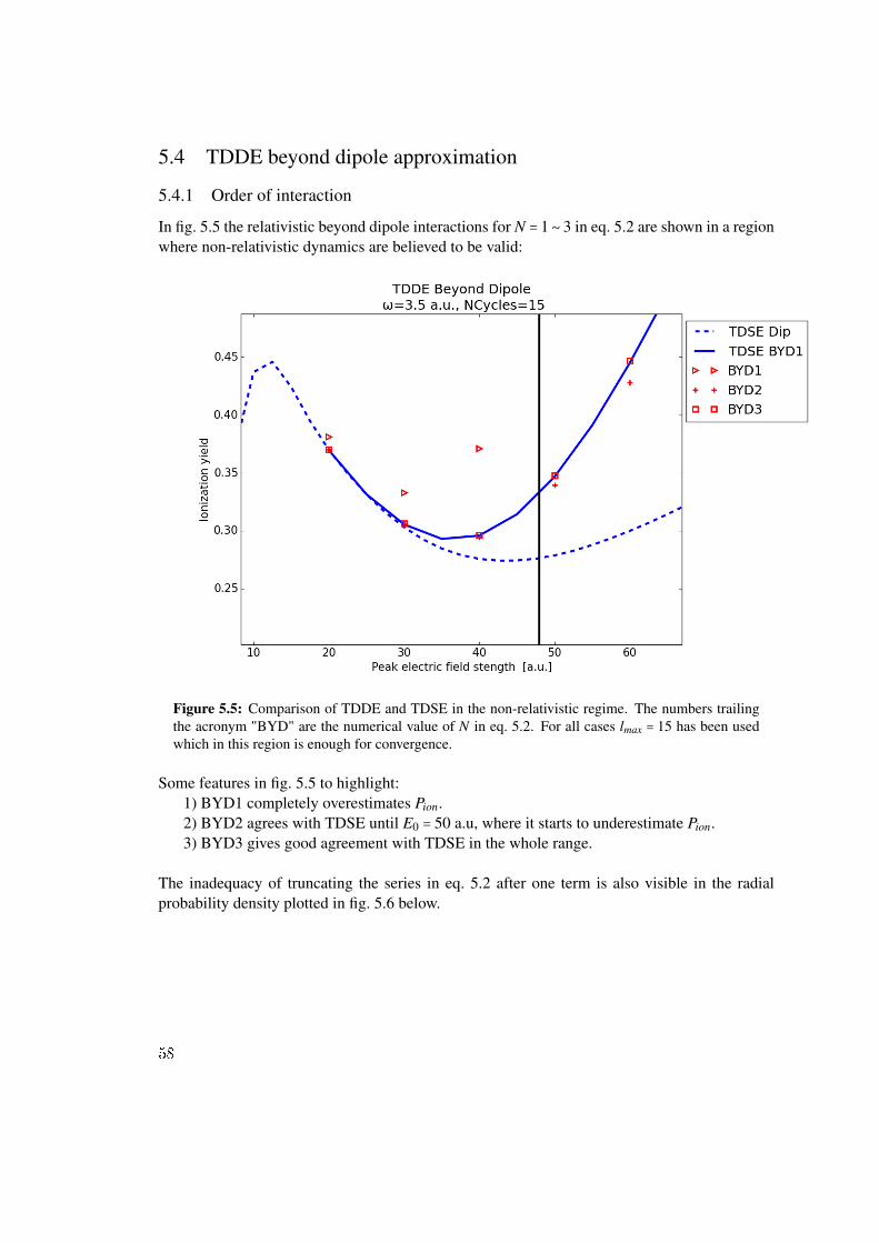
In the next section the ionization yield predicted by the relativistic Hamiltonian beyond dipoleapproximation is presented.
57
5.4 TDDE beyond dipole approximation
5.4.1 Order of interaction
In fig. 5.5 the relativistic beyond dipole interactions for N = 1 ∼ 3 in eq. 5.2 are shown in a regionwhere non-relativistic dynamics are believed to be valid:
Figure 5.5: Comparison of TDDE and TDSE in the non-relativistic regime. The numbers trailingthe acronym "BYD" are the numerical value of N in eq. 5.2. For all cases lmax = 15 has been usedwhich in this region is enough for convergence.
Some features in fig. 5.5 to highlight:1) BYD1 completely overestimates Pion.2) BYD2 agrees with TDSE until E0 = 50 a.u, where it starts to underestimate Pion.3) BYD3 gives good agreement with TDSE in the whole range.
The inadequacy of truncating the series in eq. 5.2 after one term is also visible in the radialprobability density plotted in fig. 5.6 below.
58
Figure 5.6: The radial probability distributions of the electron initially in the ground state. Thepercentage refers to elapsed interaction time. While BYD2 and BYD3 are overlapping after thepulse the wavefunction following the BYD1 Hamiltonian is visibly different. The peak electric fieldstrength is here E0 = 40.0 a.u.
Recall that complex scaling was employed to absorb outgoing flux, which in fig. 5.6 can behinted by the lack of probability towards the box end. In regards of this, the BYD1 wavefunctionis seen to be less easily killed off than BYD2 and BYD3. This is a reflection of its instability -for E0 ≥ 50 a.u. the ionization yield predicted by BYD1 even diverges, which is a consequenceof the non-Hermitian Hamiltonian that results from complex scaling.
Although not shown here, for E0 ≥ 70 a.u. BYD2 gives diverging ionization yields as well.For all values of E0 to be considered BYD3 remains non-diverging and thus showing good signsof stability for the current box.1
Before increasing the field strength further one small stop should be made.
1Note that also BYD3 would diverge at modest electric field strengths if too large values of the scalingangle or box size would be used.
59
5.4.2 Negative energy states to HD0
Throughout this thesis the importance of the negative energy states have been mentioned. Infig. 5.7 the same observation as ref [6] made can be seen:
Figure 5.7: A comparison of Pion computed with and without the time independent negative energystates in the basis.
while Pion remains (almost) the same within the dipole approximation, the BYD effects com-pletely vanish. This is not so hard to understand since the matrix elements are computed usingeq. 3.55 which connects the P(r)-component of one state with the Q(r)-component of another.Recall now the discussion following fig. 2.3: for positive energy states ∣P(r)∣ >> ∣Q(r)∣ but fornegative energy states the relation is reversed. It thus follows that the largest matrix elementsare computed between positive and negative energy states.
It should also be mentioned that for relativistic calculations in the so called length gauge, pre-dictions made within the dipole approximation are altered, see e.g ref [7].
60
5.4.3 Towards relativistic effects
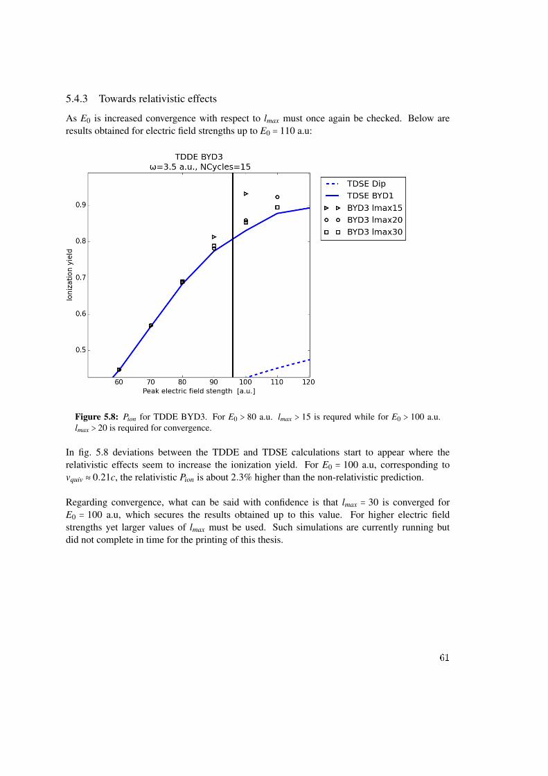
As E0 is increased convergence with respect to lmax must once again be checked. Below areresults obtained for electric field strengths up to E0 = 110 a.u:
Figure 5.8: Pion for TDDE BYD3. For E0 > 80 a.u. lmax > 15 is requred while for E0 > 100 a.u.lmax > 20 is required for convergence.
In fig. 5.8 deviations between the TDDE and TDSE calculations start to appear where therelativistic effects seem to increase the ionization yield. For E0 = 100 a.u, corresponding tovquiv ≈ 0.21c, the relativistic Pion is about 2.3% higher than the non-relativistic prediction.
Regarding convergence, what can be said with confidence is that lmax = 30 is converged forE0 = 100 a.u, which secures the results obtained up to this value. For higher electric fieldstrengths yet larger values of lmax must be used. Such simulations are currently running butdid not complete in time for the printing of this thesis.
61
62
6. Summary and Outlook
To search for relativisic effects in the dynamics induced by an attosecond pulse TDDE has beensolved for light-matter interaction beyond the dipole approximation. It has been demonstratedfrom an expansion of the vector field in the spatial coordinate
A(η) ≈A(t)+N
∑n=1
(-xc)
n 1n!
d(n)
dtn A(t)
that at least N = 3 must be used for full stability if spatial dependence of the field is to be incor-porated at all. This is in contrast to the non-relativistic TDSE for which N = 1 suffices to givethe lowest order spatial effects.
The following pulse:
A(η) = E0
ωsin2( πη
ωT)sin(η +φ) z
with ω = 3.5, T = 30π and φ = 0 was used to find at which E0 the ionization yield (Pion) given byTDDE would differ from the prediction by TDSE which then would define the threshold of therelativistic regime.
For the pulse considered in this thesis the relativistic effects start to increase Pion aroundE0 = 80 a.u, corresponding to a classical quiver velocity of the electron vquiv ≈ 0.17c. At E0 = 100a.u., corresponding to vquiv ≈ 0.21c, a difference of 2.3% is observed. For yet higher electric fieldstrengths further simulations with larger basis sets must be conducted to ensure convergence.
Once full saturation of the ionization yield is observed for the case tested in this thesis, the nextstep is naturally to repeat the process for other values of the fixed parameters. However, thereare many further applications of the program that have not yet been presented. Dynamics forhighly charged hydrogenlike systems, spin-flip studies and angular distribution of the electroncan already be computed as it is. An exciting application that requires very little extra devel-opment is the dynamics induced by multiple pulses. For instance, ref [36] considered two keVpulses with a small energy separation interacting with hydrogen. Although the electron energydistribution was dominated by two single peaks centered about each pulse energy, a small peakcentered at the energy difference of the two pulses was observed and identified to be causedby stimulated Compton scattering. The pulse parameters in their specific study were chosen tojustify non-relativistic calculations, but for yet higher energies a solution of the time dependentDirac equation is called for.
63
64
Appendix
Atomic units
Physical quantity Constant’s name SI-units Atomic unitsCharge Electron charge 1.60 ⋅10−19 C 1Mass Electron mass 9.11 ⋅1031 Kg 1
Velocity Speed of light 3.00 ⋅108 m/s 1/α ≈ 137.06
Table 6.1: Conversion table for physical quantities. α is the fine structure constant, as it is dimen-sionless it has the same value in atomic units as in SI-units.
B-splines
B-splines are piecewise polynomials of order k−1, locally confined between points defined onthe radial axis. For an non-decreasing sequence of points r0 ≤ r1 ≤ r2 ≤ . . . ,rN from r = 0 up tor = Rmax, the B-splines are generated between each point according to the recursion formula:
B1j = 1 if r j ≤ r ≤ r j+1, else B1
j = 0 (6.1)
Bkj =
r− r j
r j+k−1− r jBk−1
j (r)+r j+k − r
r j+k − r j+1Bk−1
j+1(r) (6.2)
for the j:th interval. Some properties that are worth highlighting are:
- The points can be distributed in any fashion as long as r j+1 ≥ r j.
- A B-spline of order k is confined between k+1 points. Hence the total number of B-splinesNB is of the form NB =Nint +k where Nint is the number of intervals.
- They form a complete set on the sequence.
- When evaluating integral products, such as inner products between wave functions, theirpolynomial behaviour allows for exact integration to machine accuracy using Gauss-Legendre
quadrature.
The properties listed above give quite some power to this technique. Since the points can bedistributed freely it is possible to specifically tailor the sequence to the problem at hand. Byputting densely spaced points in regions where the functions are changing rapidly and sparselyspaced points where their behaviour is more calm the dimension of the complete set NB canbe minimized without compromizing the quality of the projected function.
Figure 6.1: B-splines of orders k = 2,3,4,7 on the sequence 0,1,2,3,4. Note that order k impliespiecewise polynomials of order k−1, clearly visible k = 1,2. At each value r the B-splines sum upto unity, reflecting their completeness.
Gauge transformations in light-matter interaction
A gauge transformation in light-matter interaction is similar in spirit to the gauge transformationof the vector field encountered in chapter 3 (i.e Coulomb gauge) but in this case it is a wavefunction that is transformed. By using a suitable unitary transformation the equations of motioncan be cast on a form that is suitable for the computations to be made.
As an example, consider the following transformation that removes the A(t)2-term in ch. 3.6:
Ψ(r,t) = ei∫t
012 A(ωt′)2dt′
Ψ(r,t). (6.3)
The equation of motion 2.1 in dipole approximation is:
i∂Ψ
∂ t= [ p2
2+p ⋅A(t)+ 1
2A(t)2]Ψ
in which the wave function is replaced through 6.3:
i∂
∂ t[e−i∫
t0
12 A(t′)2dt′
Ψ(r,t)] = [ p2
2+p ⋅A(t)+ 1
2A(t)2]e−i∫
t0
12 A(t′)2dt′
Ψ(r,t) (6.4)
Carrying out the differentiation on the left hand side;
12
A(t′)2e−i∫t
012 A(t′)2dt′
Ψ(r,t)+e−i∫t
012 A(t′)2dt′ ∂ Ψ(r,t)
∂ t(6.5)
and reinserting this gives:
e−i∫t
012 A(t′)2dt′ ∂ Ψ(r,t)
∂ t= [ p2
2+p ⋅A(t)]e−i∫
t0
12 A(t′)2dt′
Ψ(r,t). (6.6)
Finding the Hermitian conjugate of U;
U = e−i∫t
012 A(t′)2dt′ →U† = ei∫
t0
12 A(t′)2dt′ (6.7)
and applying it on both sides from the left gives:
∂ Ψ(r,t)∂ t
= [ p2
2+p ⋅A(t)]Ψ(r,t). (6.8)
The last step is valid because the terms in the square brackets commute with this particular U†.This equation is equivalent to the original one and the physics described by Ψ is the same as Ψ,at least in theory. The Hamiltonian in eq. 6.8 is said to be in velocity gauge. Other gauges thatare popular are length gauge and acceleration gauge, also known as the Kramers-Hennerbergerframe [10].
If a model space is sufficiently large the numerical predictions give the correct results. Therefore,converged results computed in different gauges should agree, giving the means to test the nu-merical implementations adopted. Note also that this implies that convergence may be achievedfaster in a specific gauge, which of course is of major interest. Velocity gauge is adapted through-out this work but see [7] for a discussion on convergence behaviour in different gauges withinthe dipole approximation.
References
[1] E. GOULIELMAKIS, M. SCHULTZE, M. HOFSTETTER, V. S. YAKOVLEV, J. GAGNON, M. UIBERACKER, A. L. AQUILA,E. M. GULLIKSON, D. T. ATTWOOD, R. KIENBERGER, F. KRAUSZ, AND U. KLEINEBERG. Single-Cycle NonlinearOptics. Science, 320(5883):1614–1617, 2008. ix, 32
[2] FERENC KRAUSZ AND MISHA IVANOV. Attosecond physics. Rev. Mod. Phys., 81:163–234, Feb 2009. 13, 53
[3] V. YANOVSKY ET AL. Ultra-high intensity-300-TW laser at 0.1 Hz repetition rate. Optics Express, 16(2109), 2008. 13
[4] YOUSEF I. SALAMIN, S.X. HU, KAREN Z. HATSAGORTSYAN, AND CHRISTOPH H. KEITEL. Relativistic high-powerlaser-matter interactions. Phys. Rep., 427(2-3):41–155, 2006. 13
[5] K.Z HATSAGORTSYAN C.H.KEITEL A. DI PIAZZA, C. MÃIJLLER. Extremely high-intensity laser interactions withfundamental quantum systems. Rev. Mod. Phys., 84:1177–1226, July-Sept 2012. 13
[6] SØLVE SELSTØ, EVA LINDROTH, AND JAKOB BENGTSSON. Solution of the Dirac equation for hydrogenlike systemsexposed to intense electromagnetic pulses. Phys. Rev. A, 79(4):043418, 2009. 13, 33, 34, 44, 47, 60
[7] YULIAN V. VANNE AND ALEJANDRO SAENZ. Solution of the time-dependent Dirac equation for multiphoton ionizationof highly charged hydrogenlike ions. Phys. Rev. A, 85:033411, 2012. 44, 60, lxvii
[8] M. S. PINDZOLA AND J. A. LUDLOW. Photoionization of highly charged atomic ions. Phys. Rev. A, 81:063431, 2010.
[9] SH. A. ABDEL-NABY M. S. PINDZOLA AND F.ROBICHEAUX. Single photoionization of highly charged atomic ionsincluding the full ectromagnetic-field potential. Phys. Rev. A, 85:032701, 2012. 13
[10] B.H BRANSDEN AND 2ND EDITION C.J. JOACHAIN. Physics of Atomcs and Molecules. Prentice Hall, 2003. 15, lxvii
[11] DAVID J. GRIFFITHS. Introduction to quantum mechanics, 2nd edition. Pearson Educational International, 2005. 16, 19
[12] HARALD FRIEDRICH. Theoretical atomic physics. Springer, 2006. 17
[13] H. BACHAU, E. CORMIER, P. DECLEVA, J. E. HANSEN, AND F. MARTIN. Rep. Prog. Phys., 64:1815, 2001. 18
[14] CARL DEBOOR. A Practical Guide to Splines. Springer-Verlag, New York, 1978. 18
[15] WILLAIM T. VEETERLIN BRIAN P. FLANNERY WILLIAM H PRESS, SAUL A. TEUKOLSKY. Numerical Recipes: The Artof Scientific Computing Third Edition. Cambridge University Press, 2007. 19
[16] E. ANDERSON, Z. BAI, C. BISCHOF, S. BLACKFORD, J. DEMMEL, J. DONGARRA, J. DU CROZ, A. GREENBAUM,S. HAMMARLING, A. MCKENNEY, AND D. SORENSEN. LAPACK Users’ Guide. Society for Industrial and AppliedMathematics, Philadelphia, PA, third edition, 1999. 19, 23
[17] J. J. SAKURAI. Modern Quantum Mechanics. The Benjamin/Cummings Publishing Company, Inc., 1985. 19, 30, 43
[21] S.P GOLDMAN G.W.F DRAKE. Application of discrete-basis-set methods to the Dirac equation. Phys. Rev. A, 23, 1981.22
[22] A. D. BANDRAUK F. FILLION-GORDEAU, E. LORIN. Numerical solutions of the time-independent Dirac equation fordiatomic molecules: B splines without spurious states. Phys. Rev. A, 85:022506, 2012. 22
[23] C. FROESE-FISCHER AND O.ZATSARINNY. A B-spline Galerkin method for the Dirac equation. Computer PhysicsCommunications, 2008. 22, 27
[24] I P GRANT. B-spline methods for radial Dirac equations. Journal of Physics B, 2009. 27
[25] JOHN DAVID JACKSON. Classical electrodynamics, third edition. Wiley, 1999. 29, 33
[26] ROBIN SHAKESHAFT ALEJANDRO BUGACOV, MARCEL PONT. Possibility of breakdown of atomic stabilization in anintense high-frequency field. Phys. Rev. A Rapid communication, 48, 1993. 34
[27] I. LINDGREN AND J. MORRISON. Atomic Many-Body Theory. Series on Atoms and Plasmas. Springer-Verlag, New YorkBerlin Heidelberg, second edition, 1986. 34, 35, 39, 41
[28] MORTEN FØRRE AND ALEKSANDER SKJERLIE SIMONSEN. Nondipole ionization dynamics in atoms induced by intensexuv laser fields. Phys. Rev. A, 90:053411, 2014. 37, 53
[29] STEN SALOMONSSON ANN-MARIE MÃERTENSSON. Specific mass shift in Li and K calculated using many-body per-turbation theory. J. Phys. B, 15:2115–2130, 1982. 38
[30] JAKOB BENGTSSON, EVA LINDROTH, AND SØLVE SELSTØ. Solution of the time-dependent Schrödinger equation usinguniform complex scaling. Physical Review A, 78(3):032502, 2008. 47
[31] ARMIN SCRINZI. Infinite-range exterior complex scaling as a perfect absorber in time-dependent problems. Phys. Rev.A, 81(5):053845, May 2010. 47
[32] Y. SAAD. Analysis of some Krylov subspace approximations to the matrix exponential operator. SIAM J. Numer. Anal,29:209–228, 1992. 48
[33] E. GALLOPOULOS AND Y. SAAD. Parallel solution of parabolic equations using polynomial approximations to theexopnential. SIAM J. Numer. Anal, 13:1236–1264, 1992. 48
[34] ALEKSANDER SKJERLIE SIMONSEN AND MORTEN FØRRE. Magnetic-field-induced enhancement of atomic stabiliza-tion in intense high-frequency laser fields. Phys. Rev. A, 92:013405, 2015. 53
[35] M.GAVRILA. Atomic Stabilization in superintense laser fields. J. Phys. B, 35:R147, 2002. 56
[36] M. DONDERA H. BACHAU AND V. FLORESCU. Stimulated Compton Scattering in Two-Color Ionization of Hydrogenwith keV Electromagnetic Fields. Phys. Rev. Lett., 112:073001, 2014. 63
1
Relativistic ionization dynamics for a hydrogen atom exposed to super-intense XUV laser pulses
Tor Kjellsson,1 Sølve Selstø,2 and Eva Lindroth1
1Department of Physics, Stockholm University, AlbaNova University Center, SE-106 91 Stockholm, Sweden2Centre of Mathematics for Applications, University of Oslo, N-0316 Oslo, Norway
We study the ionization dynamics of a hydrogen atom exposed to attosecond laser pulses in the extremeultra violet region at very high intensities. The pulses are such that the electron is expected to reach relativisticvelocities, thus necessitating a full relativistic treatment. We solve the time dependent Dirac equation andcompare its predictions with those of the corresponding non-relativistic Schrodinger equation. Our findingsindicate surprisingly small relativistic corrections for cases in which free electrons are expected to be acceleratedtowards the speed of light.
PACS numbers:
I. INTRODUCTION
For lasers operating in the high intensity regime, ioniza-tion processes in which magnetic interactions play a crucialrole are seen, see, e.g., Refs. [1, 2]. At laser facilities suchas FLASH in Hamburg, such effects should also be seen forphotoionization in the ultra violet regime and beyond. Witheven stronger free electron lasers, now operating or on theirway, such at the XFEL in Germany, the SACLA in Japan andthe LCLS, USA, or the coming pan-European extreme lightinfrastructure (ELI), we expect so see experiments in whichelectrons are accelerated towards relativistic velocities in thenear future. In order to describe such processes, it is not suffi-cient for theoretical studies to just go beyond the much applieddipole approximation; a relativistic treatment based on the fullsolution of the Dirac equation is called for [3, 4].
In Ref. [5] the Dirac equation for hydrogen-like systemsexposed to strong attosecond laser pulses was solved numeri-cally. Unfortunately, for the case of hydrogen, computationalconstraints did not allow for calculations penetrating into therelativistic regime It was found, however, that even belowrelativistic velocities, the negative energy part of the energyspectrum is crucial in order to account for dynamics beyondthe dipole approximation, in which the spatial dependence ofthe external laser field is neglected all together. Moreover,in Ref. [6] it was shown that even within the dipole approxi-mation, negative energy states are crucial for ionization pro-cesses involving more than one photon. While the solutionto technical challenges regarding the Dirac equation is a goalof its own, eventually we would like to explore relativistic ef-fects. More specifically, here we investigate to what extentthe ionization probabilities predicted by the Dirac equation,differ from those of its non-relativistic counterpart, i.e., theSchrodinger equation, in a regime where relativistic correc-tions are to be expected.
Of course, relativistic effects arise when the electron isaccelerated to velocities comparable to the speed of light.This may come about in two ways; for highly charged nucleihigh velocities may be induced by the the Coulomb potentialalone, or the electron may be driven to relativistic speeds bysome external field. In the former case, relativistic correc-tions to the energy structure do of course influence the ion-ization dynamics, e.g., by modifying the ionization potential
[6–8]. However, in the present work we will restrict ourselvesto hydrogen and investigate cases in which the external fieldalone is strong enough to potentially induce relativistic dy-namics. As a measure we may take the maximum quivervelocity of a classical free electron exposed to a homoge-nous electric field of strength E0 oscillating with frequencyω: vquiv = eE0/(mω); as vquiv becomes comparable to thespeed of light c, relativistic effects are to be expected. In orderto actually see such effects in the ionization probability, thelaser specifications must, of course, be such that saturation isavoided even in this limit.
Various techniques have been applied in order to solve theDirac equation numerically, e.g., split operator methods, com-bined with Fourier transforms [8, 9] or the method of char-acteristics [10, 11], the close coupling method [7, 12] andKrylov methods [13]. In the present work the Dirac equa-tion is solved by expanding the state in a set of eigenstates ofthe light-field free Hamiltonian, as in Ref. [5, 6], and prop-agated by a low order Magnus expansion [14]. The actualmatrix exponentiation is approximated by a Krylov sub-spaceapproach as in Ref. [13]. We aim to identify relativistic ef-fects by comparing the predicted ionization probabilities withthe corresponding non-relativistic ones, which are obtained inan analogous manner.
Atomic units are used throughout unless stated otherwise.
II. THEORY
Our starting point is the time-dependent Dirac equation(TDDE):
For the representation of α, the Pauli matrices are used,
α =
(0 σσ 0
), (3)
2
and
β =
(12 00 −12
). (4)
The potential V (r) is simply the Coulomb potential froma point nucleus, i.e., we neglect retardation effects in theelectron-nucleus interaction and take the nuclear mass to beinfinite, thus allowing for separation between the electronicand the nuclear degrees of freedom. We choose to work inCoulomb gauge,∇·A = 0, with the external vector potentialA linearly polarized along the z-axis and propagating alongthe x-axis;
A(η) = A0f(η) sin(ωη + ϕ) z , (5)
where η = t−x/c. The widely applied dipole approximation,which is generally not applicable for the cases of interest here,see, e.g., the discussion by Reiss [3], consists in substituting ηwith the time t, i.e., neglecting the spatial dependence of thelaser pulse completely. The envelope function is chosen to besine-squared;
f(η) =
sin2
(πηT
), 0 < η < T
0, otherwise . (6)
To obtain the non-relativistic dynamics, the time-dependentSchrodinger equation (TDSE) must be solved:
i~d
dtΨ =
[p2
2m+ V (r) +
e
mp ·A +
e2A2
2m
]Ψ (7)
for the same vector potential.
A. Propagation and projection
The state Ψ(t) is propagated by means of a second orderMagnus propagator,
Ψ(t+ τ) = exp[−iτH(t+ τ/2)]Ψ(t) +O(τ3) . (8)
One of the major advantages of a Magnus-type propagatorfor the Schrodinger equation is stated clearly in Ref. [15]:“In contrast to standard integrators, the error does not de-pend on higher time derivatives of the solution, which is ingeneral highly oscillatory”. Due to the stiffness inherent inthe mass energy term, i.e., the mc2β term of the Hamilto-nian in Eq. (2), this becomes even more advantageous forthe Dirac equation than for the Schrodinger equation. Infact, the accuracy of many time-propagation schemes, suchas Crank-Nicholson and Runge-Kutta, suffer greatly from the2mc2 energy splitting. In Ref. [16], e.g., it is stated that“The major drawback of the Dirac treatment is the temporalstep size ∆t . ~/E required, which has to be significantlysmaller than for Schrodinger treatments, because of the largerest mass energy mc2 that is contained in the particle’s to-tal energy E.” Indeed, several works dealing numerically withTDDE apply time-steps of the order 10−5 a.u. or smaller, see,e.g., [7, 8, 11, 17]. However, for Magnus-type propagators,
lemma 4.1 of Ref. [15] provides an error bound for Eq. (8) inwhich the time-independent mass termmc2β does not enter atall, thus circumventing the above problem. Extremely smalltime steps are, of course, always required when resolving phe-nomena which really do take place at very short time scales,such as Zitterbewegung [13].
In our implementation the propagator in Eq. (8) does nottell the whole story. We have solved the Dirac equation onthe manifold consisting of only positive energy states – of thetime-dependent Hamiltonian, H(t), that is. Intuitively, thischoice may be motivated by Dirac’s original idea of the “filledsea” of negative energy states, population of such states areprohibited. We emphasize that in a time-dependent context itis crucial to keep in mind that a time dependent Hamiltonianleads to a time-dependent distinction between positive andnegative energy states; the Dirac sea is not calm, so to speak.A more technical justification for excluding negative energystates in the propagation would be that actual population ofsuch states would correspond to (real) pair production, thusnecessitating an approach based on field theory rather than aconserved number of particles. Thus, in the present regimeit should not matter whether we include them or not. In ourimplementation, however, exclusion is actually necessary dueto the use of complex scaling, see Sec. III below. Negative en-ergy states have then positive imaginary parts, which causesthe norm of the state to blow up upon application of the prop-agator in Eq. (8). We note in passing that a correct field theorytreatment of pair-production in any case would require a dis-tinction between positive and negative energy states. For thelatter to represent positrons they have to be propagated back-wards in time [18], and thus the sign of the imaginary partof the negative energy state continuum after complex rotationwould cause absorption of the positron states when they traveloutwards from the nucleus, just as is the case for the (positiveenergy) electrons.
Following the above discussion, the propagator of Eq. (8)is modified to
Ψ(t+τ) = P(t+τ/2) exp(−iτH(t+τ/2))Ψ(t)+O(t3) ,(9)
where P(t) projects the state onto the time dependent sub-space spanned by the positive spectrum of the HamiltonianH(t). This projection does not prevent the evolution from be-ing unitary.
Before we continue to the implementation of the time-dependent Dirac equation it is appropriate to discuss its non-relativistic limit since from that some numerical complica-tions that we have encountered can be understood.
B. The non-relativitic limit of the light-matter interaction
While the time-dependent Dirac equation, Eq. (1) is linearin the vector potential A, the Schrodinger equation, Eq. (7),has both a linear and a quadratic term. We can study the non-relativistic-limit of the time-dependent Dirac equation by us-ing the form of the wave function given in Eq. (15) below and
3
write Eq. (1) as:
V F + cσ · (eA + p) G = i~∂F
∂t(10)
which can be rewritten as
cσ · (eA + p)F +(V − 2mc2
)G = i~
∂G
∂t, (11)
with F and G being the large and small component, respec-tively. For the sake of simplicity, we have omitted the in-dices. Here a Foldy-Wouthuysen [19] type transformation canbe performed: From the second line one gets (keeping only thedominating term, i.e. assuming that the potential V 2mc2,and that the time variation of the small component is modest)
G ≈ 1
2mcσ · (eA + p)F. (12)
and inserting this on the first line we get
V F +1
2m(σ · (eA + p))
2F = i~
∂F
∂t(V +
1
2m(eA + p)
2+
e~2m
σ ·B)F = i~
∂F
∂t, (13)
where again the A2-term is reappearing. We see that the A2-term is implicitly present in the Dirac equation and enters theequation for the large component of the wave function throughthe small component. Whenever we try to formulate the inter-action with the electromagnetic field through operators thatare diagonal with respect to the small and large componentit reappears. A practical consequence of this is that when thespatial dependence of A is included to a specific order througha Taylor expansion, cf. Sec. III A, the implicit A2-term willalways be included to the square of this order. As a result,higher order contributions in this expansion are needed for thesolution of the Dirac equation than previously was found forthe Schrodinger equation [20].
III. IMPLEMENTATION
We expand our wave function in eigenstates of the unper-turbed Hamiltonian H0,
Ψ(t) =∑
n,j,m,κ
cn,j,m,κψn,j,m,κ , (14)
with
ψn,j,m,κ(r) =
(Fn,j,m,κ(r)Gn,j,m,κ(r)
), (15)
where(Fn,j,m,κ(r)Gn,j,m,κ(r)
)=
1
r
(Pn,κ(r)Xκ,j,m(Ω)iQn,κ(r)X−κ,j,m(Ω)
). (16)
Here κ = l for j = l − 1/2 and κ = −(l + 1) for j =l + 1/2, and Xκ,j,m represents the spin-angular part whichhas the analytical form:
Xκ,j,m =∑ms,ml
〈lκ,ml; s,ms|j,m〉Y lκml(θ, φ)χms (17)
where Y lκml(θ, φ) is a spherical harmonic and χms is an eigen-spinor. The radial components Pn,κ(r) and Qn,κ(r) are ex-panded in B-splines [21];
Pn,κ(r) =∑i
aiBk1i (r) Qn,κ(r) =
∑j
bjBk2j (r).
(18)Ref [22] has demonstrated that specific choices of B-spline
orders k1 and k2 controls the occurrence of the so-called spu-rious states, that are known to appear in the numerical spec-trum after discretization of the Dirac Hamiltonian. Whilethe choice k1 = k2 contaminates the spectrum with spuri-ous states the choices k1 = k2 ± 1 are reported to be stablecombinations that do not produce them.
The energy index n corresponds to both bound and pseudocontinuum states, with the latter referring to both the nega-tive and the positive energy continuum. In general a ratherlarge number of continuum states are necessary in order toachieve convergent results. This number is however drasti-cally reduced by imposing complex scaling of the spatial co-ordinates,
r → r exp(iθ), with 0 ≤ θ ≤ π/4 . (19)
This renders the energies of bound states unaffected whilecontinuum energies acquire an imaginary contribution which,effectively, broadens the energy of these states. Thus, the en-tire energy range is well represented by very few states [23].The price to be paid for this advantage is that, numerically, welose information about the photo electron after ionization.
A. Interaction
With the pulse linearly polarized in z the time dependentpart of the Hamiltonian becomes HI(t) = cαzA(η). As thisterm depends on both time and space, t and x, a direct calcu-lation of such couplings would have to be performed at eachand every time step in order to represent H(t) numerically.This cumbersome feature may be removed by factorizing thevector potential in a time-dependent and a spatially dependentpart,
A(η) ≈ntrunc∑n=0
anT (t)X(x) . (20)
By determining the couplings αzX(x) the numerical repre-sentation at any time is easily constructed by the above ex-pansion. Such separations may be achieved by, e.g., a Fourierexpansion in η or a Taylor expansion in x. In Ref. [5] bothmethods were used. In the Fourier implementation, the num-ber of terms was minimized in two ways: First, by taking Ato have the pulse length T as period and, second, by neglect-ing the spatial dependence of the envelope f(η), c.f., Eq. (6).Both of these approaches have severe shortcomings.
Thus we resort to a Taylor expansion in the present work:
A(η) ≈ntrunc∑n=0
1
n!A(n)(t)
(-x
c
)n. (21)
4
Expressing xn as a sum of spherical harmonics Y λµ :
xn =∑i
cirnY λµ (22)
the interaction operator is given by terms of the form:
〈nκjm|αzrγY λµ |nκjm〉 =
i
∫r
[P ∗nκ(r)rγQnκ(r)〈κjm|σ1
0Yλµ |-κjm〉−
Q∗nκ(r)rγPnκ(r)〈-κjm|σ10Y
λµ |κjm〉
]dr. (23)
With the radial components expressed in B-splines, the in-tegrals are computed to machine accuracy using Gauss-Legendre quadrature. To obtain the spin-angular part, the op-erator product can be expressed in a coupled tensor operatorbasis:
σ10Y
λµ =
λ+1∑K=|λ−1|
〈10;λµ|KQ〉σσσ1Yλ
KQ, Q = −µ
With this choice the spin-angular part may be computed as:
〈κjm|σ10Y
λµ |κjm〉 =
λ+1∑K=|λ−1|
(-1)λ−1−Q√
2K + 1
×(
1 λ K0 µ −µ
)〈κjm|
σσσ1Yλ
KQ|κjm〉 (24)
The Wigner-Eckart theorem can be applied to the matrix ele-ment of the combined operator
σσσ1Yλ
KQ
:
〈κjm|σσσ1Yλ
KQ|κjm〉 =
(-1)j−m
(j K j−m Q m
)〈j||σσσ1Yλ
K ||j〉 (25)
with the reduced matrix element given by:
〈j||σσσ1Yλ
K ||j〉 =
√(2j + 1)(2K + 1)(2j + 1)
×〈s||σσσ1||s〉〈l||Yλ||l〉
l l 1s s λ
j J K
. (26)
With this scheme the couplings induced by αzxn, for n =0, 1, . . . , ntrunc are readily computed.
B. Non-relativistic interaction
The non-relativistic spectral basis has eigenfunctions of theform
Φ(r) =Pnl(r)
rY lm(θ, φ) (27)
where just like the relativistic case, the radial component isexpanded in B-splines while the angular part is analyticallyknown.
The time-dependent Schrodinger equation is given inEq. (7), and also here the form of the vector field in Eq. (21)will be used. Typically, the A2 term provides practically allcorrections to the dipole approximation [20, 24] so to first or-der (which Ref. [20] found sufficient) in x we have:
HNR ≈p2
2m+ V (r) +
e
mpzA(t)− e2
m
x
cA(t)A(1)(t) (28)
where the purely time dependent A(t)2 has been removed bythe gauge transformation:
Ψ(r, t) = ei~∫ t0e2
2mA(ωt′)2dt′Ψ(r, t). (29)
The pz-couplings are given by:
〈nalama|pz|nblbmb〉 =
(-1)la−ma
(la 1 lb
-ma 0 mb
)〈nala||p1||nblb〉 (30)
while the x-couplings are computed as:
〈nalama|x|nblbmb〉 =√2π
3· (-1)
la−ma((
la 1 lb-ma -1 mb
)−(la 1 lb
-ma 1 mb
))×〈nala||rY1||nblb〉.
(31)
C. Propagation
The main drawback of the propagator projected onto thepositive energy spectrum of the Hamiltonian H(t), given inEq. (9) is the need for a full diagonalization of the Hamilto-nian at each and every time step. This is not only required inorder to exponentiate the Hamiltonian but also to distinguishbetween positive and negative energy states so that the pro-jection P can be performed. To this end, Krylov subspacemethods are quite useful [13, 25]. Such methods provide ac-curate approximations to the action of an exponential of anoperator on a specific vector. Moreover, they may typically beimplemented numerically very efficiently. At each time stepthe Krylov subspace of dimension m, Km(t), is spanning theset of states obtained by iteratively multiplying the state withthe Hamiltonian,
[H(t+ τ/2)]n
Ψ(t), n = 0, ..., (m− 1) . (32)
Instead of diagonalizing the full Hamiltonian, we diagonalizeits projection into K(t) – with the dimension m considerablysmaller than the full dimension of the numerical problem. Infact, high accuracy is achieved with surprisingly low m. Byexponentiating and projecting according to Eq. (9), propaga-tion is performed within K(t), and the approximate state vec-tor at time t + τ is constructed by transforming back to theoriginal Hilbert space.
5
To decrease memory consumption H(t + τ/2) is actuallynever explicitly built even in sparse form but its action isaccounted for by directly operating with couplings and timefactors on Ψ(t). The bottleneck is then no longer the diago-nalization but the operations representing the matrix-vectorproduct in Eq. 32. To reduce the computational time theoperations are distributed to several processing units.
D. The representation of the vector field beyond the dipoleapproximation
As discussed above we have chosen to represent the vec-tor field through a Taylor expansion, see Eq. 21. Ref. [20],which considered the time-dependent Schrodinger equation,provides strong support that below the relativistic region, thefirst order term alone (i. e. ntrunc = 1) provides practicallyall corrections to the dipole prediction. At first sight there isno a priori reason why this conclusion should not apply to therelativistic situation as well. Yet, we typically have to resortto a third order expansion in our calculations. The underly-ing problem is the implicit inclusion of the A2 term in theDirac-equation, discussed in Sec.II B above. When only firstorder corrections to A are included some of the second or-der corrections in the implicit A2-term will still be included,namely the ∼ (A(1))2x2 contributions, while others, namelythe ∼ A(2)A(0)x2 contributions, require the inclusion also ofsecond order corrections to A. We note that Førre and Si-monsen [20] has shown that in the non-relativistic limit thereare important cancellations between the x2-terms. It is thusnatural to assume that these cancellations are a key-issue andthat higher-order correction terms to A are needed to achievethem when using the Dirac equation [26]. The fact that theinstability problem is drastically reduced when higher ordersof x is included in Eq. (21) supports this conclusion.
The solution of the TDSE has been done along the samelines as that of the TDDE.
IV. RESULTS AND DISCUSSION
For the relativistic basis we use B-splines of orders k1 = 7,k2 = 8 and apply the boundary conditions:
For the non-relativistic basis we choose k = 7 and
Pn,l(0) = Pn,l(rmax) = 0 . (34)
The ionization probability, Pion, of the hydrogen atom groundstate electron after interaction with a pulse having the fixedparameters:
ω = 3.5, φ = 0, T = 2πNc, Nc = 15 (35)
has been studied as a function of E0. The calculations are car-ried out in a box of rmax = 40 a.u. using 120 B-splines and a
uniform complex scaling angle θ = 2.5 to avoid artificial re-flection at the box end. This choice is motivated by the recentnon-relativistic study in Ref. [27] where a similar box wasused for pulses with the same central frequency, a maximumelectric field strengths up to 60 a.u. and number of optical cy-cles up to Nc = 100. Although the maximum electric fieldstrength considered in this work is E0 = 110 a.u., the muchshorter pulses, and thus also propagation times, should ensurethat the box is adequate to describe the ionization dynamics.
We have studied the predictions of the ionization probabil-ity, Pion, and compared the results obtained by the TDSE andTDDE. In all computations convergence with respect to themaximum orbital angular momentum included, lmax, havebeen checked.
In Fig. 1 the relativistic and non-relativistic ionization prob-ability, Pion, computed within the dipole approximation areshown. For low field strengths the ionization probability is in-creasing linearly with increasing field strength, but for aroundE0 ≈ 10 a.u. the so-called stabilization against ionization setsin [28]. For even higher field strengths the ionization startsto increase again. Although, as will be seen in Fig. 2, the
FIG. 1: Comparison of TDSE and TDDE calculations within thedipole approximation. Each vertical line corresponds to an incrementof vquiv = 0.1c. A difference is emerging at about E0 = 70 a.u.,corresponding to vq ≈ 0.15c. Both simulations have been carriedout with lmax = 40.
dipole approximation in itself is not valid for regions wherevquiv > 0.15c, it is interesting to note that the relativistic ef-fect seem to result in a tiny suppression of the ionization yield.
In Fig. 2 the results from solutions of the TDDE using theTaylor expansion of the vector field, Eq. 21, with ntrunc =1− 3 are shown on top of the non-relativistic calculations forE0 ≤ 60 a.u. Note that the dipole approximation is breakingdown for E0 ≥ 30 a.u. The effects beyond the dipole ap-proximation causes the ionization yield to increase further forhigher strengths, the physics behind this behaviour has beendiscussed in Ref. [27].
The vertical line denotes the electric field strength corre-sponding to a quiver velocity of the electron vquiv = 0.1c.
6
FIG. 2: Comparison of TDDE and TDSE in the non-relativisticregime. The numbers trailing the acronym ”BYD” are the numer-ical value of ntrunc in eq. 21. For all cases lmax = 15 have beenused. The parameters are the same as in Fig. 1
For electric field strengths below and slightly above this valuethe TDSE and TDDE should agree. However, the relativisticfirst order approximation of the spatial dependence severelyoverestimates the ionization yield. Addition of the second or-der corrections gives initial agreement but is then seen to un-derestimate the Pion predicted by TDSE. Finally, inclusion ofalso the third order term in eq. 21 gives excellent agreementwith TDSE up to E0 = 60 a.u. Thus, relativistic effects mustcome in play at yet higher field strengths.
We note that the smoother behaviour of the TDDE resultswith increasing spatial order in the vector field supports theargument made in section II B - there is clearly a complicatedimplicit inclusion of higher order terms in the TDDE whena certain order of the Taylor expansion of the vector field,Eq. (21) is employed.
A. Removing time independent negative energy states
In Ref. [5] it was shown that exclusion of the time-independent negative-energy states from the propagation ba-sis removed all effects beyond the dipole approximation buthad no effect within the dipole approximation. As a furtherdemonstration of this the TDDE calculations within the dipoleapproximation, as well as calculations including the first andthird order corrections to this approximation, was repeatedwithout the time independent negative energy states. In Fig. 3it is seen that these three different Hamiltonians now give thesame ionization probability, Pion.
B. Relativistic effects
For relativistic effects to become visible E0 must now befurther increased. As this is done convergence with respect tolmax must once again be checked. Fig. 4 shows results ob-tained for electric field strengths up to E0 = 110 a.u. For
FIG. 3: A comparison of the ionization probability, Pion, computedwith and without the time-independent negative-energy states in thebasis.
E0 = 80 a.u the three TDDE curves with lmax = 15, 20, 30converge slightly above the TDSE curve. This indicates thatthere is a small relativistic shift emerging here where vquiv ≈0.17c. When we increase the field strength even more theionization probabilities, Pion, predicted by TDDE and TDSEseparate further, suggesting that the relativistic effect is in-creasing the ionization yield, rather than decreasing it as pre-dicted within the dipole approximation.
FIG. 4: Comparison of TDSE and TDDE for higher peak-values ofthe electromagnetic field, E0. The vertical line indicates vquiv =0.2c.
V. CONCLUSION
We have solved the time-dependent Dirac equation for a hy-drogen atom exposed to extreme laser pulses. Upon compari-son with the non-relativistic counterpart, i.e., the Schrodingerequation, it was found that effects beyond the dipole approx-imation are more complicated to incorporate correctly in therelativistic framework. Whereas first order space-dependentcorrections to the vector field are sufficient for TDSE, TDDEdemands an expansion to at least third order for convergence.Regarding the ionization yield, tiny relativistic effects for thetest case start to appear for a quiver velocity of vquiv ≈ 0.17c.
7
The relativistic corrections to Pion at E0 = 110 a.u, corre-sponding to vquiv ≈ 0.23c, is about 2%.
Acknowledgments
The authors would like to thank M. Førre for fruitful discus-sions and for providing us with data for comparison. Compu-
tations were performed at the cloud computing facility “Alto”at Oslo and Akershus University College of Applied Sciences.Financial support by the Swedish Research Council (VR) isgratefully acknowledged.
[1] C. I. Moore, A. Ting, S. J. McNaught, J. Qiu, H. R. Burris, andP. Sprangle, Phys. Rev. Lett. 82, 1688 (1999).
[2] C. T. L. Smeenk, L. Arissian, B. Zhou, A. Mysyrowicz, D. M.Villeneuve, A. Staudte, and P. B. Corkum, Phys. Rev. Lett. 106,193002 (2011).
[3] H. R. Reiss, Phys. Rev. A 63, 013409 (2000).[4] A. Di Piazza, C. Muller, K. Z. Hatsagortsyan, and C. H. Keitel,
Rev. Mod. Phys. 84, 1177 (2012).[5] S. Selstø, E. Lindroth, and J. Bengtsson, Phys. Rev. A 79,
043418 (2009).[6] Y. V. Vanne and A. Saenz, Phys. Rev. A 85, 033411 (2012).[7] M. S. Pindzola, J. A. Ludlow, and J. Colgan, Phys. Rev. A 81,
063431 (2010).[8] H. Bauke, H. G. Hetzheim, G. R. Mocken, M. Ruf, and C. H.
Keitel, Phys. Rev. A 83, 063414 (2011).[9] G. R. Mocken and C. H. Keitel, Comput. Phys. Comm. 178,
868 (2008).[10] F. Fillion-Gourdeau, E. Lorin, and A. D. Bandrauk, Comput.
Phys. Comm. 183, 1403 (2012).[11] F. Fillion-Gourdeau, E. Lorin, and A. D. Bandrauk, J. Comp.
Phys. 272, 559 (2014).[12] M. S. Pindzola, S. A. Abdel-Naby, F. Robicheaux, and J. Col-
gan, Phys. Rev. A 85, 032701 (2012).[13] R. Beerwerth and H. Bauke, Comput. Phys. Comm. 188, 189
(2015).
[14] S. Blanes, F. Casas, J. Oteo, and J. Ros, Physics Reports 470,151 (2009).
[15] M. Hochbruck and C. Lubich, SIAM J. Numer. Anal. 41, 945(2003).
[16] Y. I. Salamin, S. Hu, K. Z. Hatsagortsyan, and C. H. Keitel,Phys. Rep. 427, 41 (2006).
[17] G. R. Mocken and C. H. Keitel, Phys. Rev. Lett. 91, 173202(2003).
[18] R. P. Feynman, Phys. Rev. 76, 749 (1949).[19] L. L. Foldy and S. A. Wouthuysen, Phys. Rev. 78, 29 (1950).[20] M. Førre and A. S. Simonsen, Phys. Rev. A 90, 053411 (2014).[21] C. de Boor, A Practical Guide to Splines (Springer-Verlag,
1978), revised edition 2001 ed.[22] C. F. Fischer and O. Zatsarinny, Comput. Phys. Comm. 180,
879 (2009).[23] J. Bengtsson, E. Lindroth, and S. Selstø, Phys. Rev. A 78,
032502 (2008).[24] K. J. Meharg, J. S. Parker, and K. T. Taylor, J. Phys. B 38, 237
(2005).[25] M. Hochbruck and C. Lubich, SIAM J. Numer. Anal. 34, 1911
(1997).[26] M. Førre, private communication (2015).[27] A. S. Simonsen and M. Førre, Phys. Rev. A 92, 013405 (2015).[28] M. Gavrila, J. Phys. B 35, R147 (2002).