The Astrophysical Journal, 720:205–225, 2010 September 1 doi:10.1088/0004-637X/720/1/205 C 2010. The American Astronomical Society. All rights reserved. Printed in the U.S.A. RELATIVISTIC LINES AND REFLECTION FROM THEINNER ACCRETION DISKS AROUND NEUTRON STARS Edward M. Cackett 1 ,8 , Jon M. Miller 1 , David R. Ballantyne 2 , Didier Barret 3 , Sudip Bhattacharyya 4 , Martin Boutelier 3 , M. Coleman Miller 5 , Tod E. Strohmayer 6 , and Rudy Wijnands 7 1 Department of Astronomy, University of Michigan, Ann Arbor, MI 48109, USA; [email protected]2 Center for Relativistic Astrophysics, School of Physics, Georgia Institute of Technology, Atlanta, GA 30332, USA 3 Centre d’Etude Spatiale des Rayonnements, CNRS/UPS, 9 Avenue du Colonel Roche, 31028 Toulouse Cedex04, France 4 Department of Astronomy and Astrophysics, Tata Institute of Fundamental Research, Mumbai 400005, India 5 Department of Astronomy, University of Maryland, College Park, MD 20742-2421, USA 6 Astrophysics Science Division, NASA/GSFC, Greenbelt, MD 20771, USA 7 Astronomical Institute “Anton Pannekoek,” University of Amsterdam, Science Park 904, 1098 XH, Amsterdam, The Netherlands Received 2009 August 9; accepted 2010 July 4; published 2010 August 6 ABSTRACT A number of neutron star low-mass X-ray binaries (LMXBs) have recently been discovered to show broad, asymmetric Fe K emission lines in their X-ray spectra. These lines are generally thought to be the most prominent part of a reflection spectrum, originating in the inner part of the accretion disk where strong relativistic effects can broaden emission lines. We present a comprehensive, systematic analysis of Suzaku and XMM-Newton spectra of 10 neutron star LMXBs, all of which display broad Fe K emission lines. Of the 10 sources, 4 are Z sources, 4 are atolls, and 2 are accreting millisecond X-ray pulsars (also atolls). The Fe K lines are fit well by a relativistic line model for a Schwarzschild metric, and imply a narrow range of inner disk radii (6–15 GM/c 2 ) in most cases. This implies that the accretion disk extends close to the neutron star surface over a range of luminosities. Continuum modeling shows that for the majority of observations, a blackbody component (plausibly associated with the boundary layer) dominates the X-ray emission from 8 to 20 keV. Thus it appears likely that this spectral component produces the majority of the ionizing flux that illuminates the accretion disk. Therefore, we also fit the spectra with a blurred reflection model, wherein a blackbody component illuminates the disk. This model fits well in most cases, supporting the idea that the boundary layer illuminates a geometrically thin disk. Key words: accretion, accretion disks – stars: neutron – X-rays: binaries 1. INTRODUCTION X-ray emission lines from the innermost accretion disks are well known in supermassive and stellar-mass black holes, where they are shaped by relativistic effects (for a review, see Miller 2007). The utility of such lines is two-fold: they can be used to constrain the spin of the black hole, and they can be used to constrain the nature of the innermost accretion flow, particularly the proximity of the disk to the black hole (Brenneman & Reynolds 2006; Miniutti et al. 2009; Reis et al. 2009a; Miller et al. 2006a, 2008b, 2009; Reynolds et al. 2009; Wilkinson & Uttley 2009; Schmoll et al. 2009; Fabian et al. 2009). Disk lines are produced in a fairly simple manner: a source of hard X-ray emission that is external to the disk is all that is re- quired. The specific nature of the hard X-ray emission—whether thermal or non-thermal, whether due to Compton upscattering (e.g., Gierli´ nski et al. 1999) or emission from the base of a jet (Markoff & Nowak 2004; Markoff et al. 2005), or even a hot blackbody—is less important than the simple fact of a contin- uum source with substantial ionizing flux. The most prominent line produced in this process is typically an Fe K line, due to its abundance and fluorescent yield; however, other lines can also be produced. The overall interaction is known as “disk reflection” and more subtle spectral features, including a “reflection hump” peaking between 20 and 30 keV, are also expected (see, e.g., George & Fabian 1991; Magdziarz & Zdziarski 1995; Nayak- shin & Kallman 2001; Ballantyne et al. 2001; Ross & Fabian 2007). 8 Chandra Fellow. Largely owing to a combination of improved instrumentation and concerted observational efforts within the last two years, asymmetric Fe K disk lines have been observed in eight neutron star low-mass X-ray binaries (LMXBs; Bhattacharyya & Strohmayer 2007; Cackett et al. 2008; Pandel et al. 2008; D’A` ı et al. 2009; Cackett et al. 2009a; Papitto et al. 2009; Shaposhnikov et al. 2009; Reis et al. 2009b; Di Salvo et al. 2009c; Iaria et al. 2009). In the case of neutron stars, disk lines can be used in much the same way as in black holes to determine the inner disk radius. The radius of a neutron star is critical to understanding its equation of state; disk lines set an upper limit since the stellar surface (if not also a boundary layer) truncates the disk. In the case of neutron stars harboring pulsars, disk lines can be used to trace the radial extent of the disk and to obtain a magnetic field constraint (Cackett et al. 2009a). Finally, in a number of neutron stars, hot quasi-blackbody emission (potentially from the boundary layer) provides most of the flux required to ionize iron; the fact that the disk intercepts this flux suggests that the inner disk is geometrically thin, or at least thinner than the vertical extent of the boundary layer. Disk line spectroscopy provides an independent view on the inner accretion flow in neutron star LMXBs, wherein some constraints have been derived using X-ray timing (for a review, see van der Klis 2006). The higher frequency part of so-called kHz quasi-periodic oscillation (QPO) pairings may reflect the Keplerian orbital frequency in the inner disk (e.g., Stella & Vietri 1998), for instance. Trends in the coherence of the low- frequency part of kHz QPO pairs may indicate the point at which the disk has reached an inner stable orbit (Barret et al. 2006), though see M´ endez (2006) for an opposing view. Thus, 205
RELATIVISTIC LINES AND REFLECTION FROM THE INNER ACCRETION DISKS AROUNDNEUTRON STARS
Edward M. Cackett1,8
, Jon M. Miller1, David R. Ballantyne
2, Didier Barret
3, Sudip Bhattacharyya
4,
Martin Boutelier3, M. Coleman Miller
5, Tod E. Strohmayer
6, and Rudy Wijnands
71 Department of Astronomy, University of Michigan, Ann Arbor, MI 48109, USA; [email protected]
2 Center for Relativistic Astrophysics, School of Physics, Georgia Institute of Technology, Atlanta, GA 30332, USA3 Centre d’Etude Spatiale des Rayonnements, CNRS/UPS, 9 Avenue du Colonel Roche, 31028 Toulouse Cedex04, France
4 Department of Astronomy and Astrophysics, Tata Institute of Fundamental Research, Mumbai 400005, India5 Department of Astronomy, University of Maryland, College Park, MD 20742-2421, USA
6 Astrophysics Science Division, NASA/GSFC, Greenbelt, MD 20771, USA7 Astronomical Institute “Anton Pannekoek,” University of Amsterdam, Science Park 904, 1098 XH, Amsterdam, The Netherlands
Received 2009 August 9; accepted 2010 July 4; published 2010 August 6
ABSTRACT
A number of neutron star low-mass X-ray binaries (LMXBs) have recently been discovered to show broad,asymmetric Fe K emission lines in their X-ray spectra. These lines are generally thought to be the most prominentpart of a reflection spectrum, originating in the inner part of the accretion disk where strong relativistic effects canbroaden emission lines. We present a comprehensive, systematic analysis of Suzaku and XMM-Newton spectra of10 neutron star LMXBs, all of which display broad Fe K emission lines. Of the 10 sources, 4 are Z sources, 4are atolls, and 2 are accreting millisecond X-ray pulsars (also atolls). The Fe K lines are fit well by a relativisticline model for a Schwarzschild metric, and imply a narrow range of inner disk radii (6–15 GM/c2) in mostcases. This implies that the accretion disk extends close to the neutron star surface over a range of luminosities.Continuum modeling shows that for the majority of observations, a blackbody component (plausibly associatedwith the boundary layer) dominates the X-ray emission from 8 to 20 keV. Thus it appears likely that this spectralcomponent produces the majority of the ionizing flux that illuminates the accretion disk. Therefore, we also fit thespectra with a blurred reflection model, wherein a blackbody component illuminates the disk. This model fits wellin most cases, supporting the idea that the boundary layer illuminates a geometrically thin disk.
X-ray emission lines from the innermost accretion disks arewell known in supermassive and stellar-mass black holes, wherethey are shaped by relativistic effects (for a review, see Miller2007). The utility of such lines is two-fold: they can be usedto constrain the spin of the black hole, and they can be used toconstrain the nature of the innermost accretion flow, particularlythe proximity of the disk to the black hole (Brenneman &Reynolds 2006; Miniutti et al. 2009; Reis et al. 2009a; Milleret al. 2006a, 2008b, 2009; Reynolds et al. 2009; Wilkinson &Uttley 2009; Schmoll et al. 2009; Fabian et al. 2009).
Disk lines are produced in a fairly simple manner: a source ofhard X-ray emission that is external to the disk is all that is re-quired. The specific nature of the hard X-ray emission—whetherthermal or non-thermal, whether due to Compton upscattering(e.g., Gierlinski et al. 1999) or emission from the base of a jet(Markoff & Nowak 2004; Markoff et al. 2005), or even a hotblackbody—is less important than the simple fact of a contin-uum source with substantial ionizing flux. The most prominentline produced in this process is typically an Fe K line, due to itsabundance and fluorescent yield; however, other lines can also beproduced. The overall interaction is known as “disk reflection”and more subtle spectral features, including a “reflection hump”peaking between 20 and 30 keV, are also expected (see, e.g.,George & Fabian 1991; Magdziarz & Zdziarski 1995; Nayak-shin & Kallman 2001; Ballantyne et al. 2001; Ross & Fabian2007).
8 Chandra Fellow.
Largely owing to a combination of improved instrumentationand concerted observational efforts within the last two years,asymmetric Fe K disk lines have been observed in eightneutron star low-mass X-ray binaries (LMXBs; Bhattacharyya& Strohmayer 2007; Cackett et al. 2008; Pandel et al. 2008;D’Aı et al. 2009; Cackett et al. 2009a; Papitto et al. 2009;Shaposhnikov et al. 2009; Reis et al. 2009b; Di Salvo et al.2009c; Iaria et al. 2009). In the case of neutron stars, disk linescan be used in much the same way as in black holes to determinethe inner disk radius. The radius of a neutron star is critical tounderstanding its equation of state; disk lines set an upper limitsince the stellar surface (if not also a boundary layer) truncatesthe disk. In the case of neutron stars harboring pulsars, disklines can be used to trace the radial extent of the disk and toobtain a magnetic field constraint (Cackett et al. 2009a). Finally,in a number of neutron stars, hot quasi-blackbody emission(potentially from the boundary layer) provides most of the fluxrequired to ionize iron; the fact that the disk intercepts this fluxsuggests that the inner disk is geometrically thin, or at leastthinner than the vertical extent of the boundary layer.
Disk line spectroscopy provides an independent view on theinner accretion flow in neutron star LMXBs, wherein someconstraints have been derived using X-ray timing (for a review,see van der Klis 2006). The higher frequency part of so-calledkHz quasi-periodic oscillation (QPO) pairings may reflect theKeplerian orbital frequency in the inner disk (e.g., Stella &Vietri 1998), for instance. Trends in the coherence of the low-frequency part of kHz QPO pairs may indicate the point atwhich the disk has reached an inner stable orbit (Barret et al.2006), though see Mendez (2006) for an opposing view. Thus,
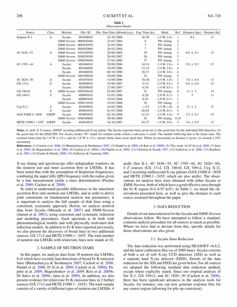
Notes. A: atoll, Z: Z source, AMXP: accreting millisecond X-ray pulsar. The Suzaku exposure times given are (1) the good time for the individual XIS detectors, (2)the good time for the HXD/PIN. For Suzaku modes “W” stands for window-mode (where a sub-array is used). The number following that is the frame time. Thenominal frame time for 1/4 W is 2.0 s, and for 1/8 W is 1.0 s, shorter frame times incur dead time. Where no uncertainty in distance is given, we assume a 25%uncertainty.References. (1) Cackett et al. 2008, (2) Bhattacharyya & Strohmayer 2007, (3) Pandel et al. 2008, (4) Reis et al. 2009b, (5) This work, (6) D’Aı et al. 2009, (7) Iariaet al. 2009, (8) Shaposhnikov et al. 2009, (9) Cackett et al. 2009a, (10) Papitto et al. 2009, (11) Christian & Swank 1997, (12) Galloway et al. 2008, (13) Kuulkerset al. 2003, (14) Fender & Hendry 2000, (15) Galloway & Cumming 2006.
X-ray timing and spectroscopy offer independent windows onthe neutron star and inner accretion flow in LMXBs. It hasbeen noted that with the assumption of Keplerian frequencies,combining the upper kHz QPO frequency with the radius givenby a line measurement yields a mass determination (Pirainoet al. 2000; Cackett et al. 2008).
In order to understand possible differences in the innermostaccretion flow onto neutron star LMXBs, and in order to derivejoint constraints on fundamental neutron star parameters, itis important to analyze the full sample of disk lines using aconsistent, systematic approach. Herein, we analyze archivaldata from Suzaku (Mitsuda et al. 2007) and XMM-Newton(Jansen et al. 2001), using consistent and systematic reductionand modeling procedures. Each spectrum is fit both withphenomenological models and with physically motivated diskreflection models. In addition to Fe K lines reported previously,we also present the discovery of broad lines in two additionalsources, GX 17+2 and HETE J1900.1−2455. The total numberof neutron star LMXBs with relativistic lines now stands at 10.
2. SAMPLE OF NEUTRON STARS
In this paper, we analyze data from 10 neutron star LMXBs,8 of which have recently had detections of broad Fe K emissionlines (Bhattacharyya & Strohmayer 2007; Cackett et al. 2008;Pandel et al. 2008; D’Aı et al. 2009; Cackett et al. 2009a; Pa-pitto et al. 2009; Shaposhnikov et al. 2009; Reis et al. 2009b;Di Salvo et al. 2009c; Iaria et al. 2009). In addition, we alsopresent evidence for relativistic Fe K emission lines in 2 furthersources (GX 17+2 and HETE J1900.1−2455). The total sampleconsists of a variety of different types of neutron star LMXBs: 4
atolls (Ser X-1, 4U 1636−53, 4U 1705−44, 4U 1820−30),4 Z sources (GX 17+2, GX 340+0, GX 349+2, Cyg X-2),and 2 accreting millisecond X-ray pulsars (SAX J1808.4−3658and HETE J1900.1−2455, which are also atolls). The obser-vations we analyze here were obtained with either Suzaku orXMM-Newton, both of which have a good effective area throughthe Fe K region (6.4–6.97 keV). In Table 1, we detail the ob-servations presented here, as well as give the distance to eachsource assumed throughout the paper.
3. DATA REDUCTION
Details of our data reduction for the Suzaku and XMM-Newtonobservations follow. We have attempted to follow a standard,common analysis procedure for all sources as much as possible.Where we have had to deviate from this, specific details forthose observations are also given.
3.1. Suzaku Data Reduction
The data reduction was performed using HEASOFT v6.6.2,and the latest calibration files (as of 2009 June). Suzaku consistsof both a set of soft X-ray CCD detectors (XIS) as well asa separate hard X-ray detector (HXD). Details of the datareduction for the XIS and HXD are given below. For all sourceswe adopted the following standard data reduction method,except where explicitly stated. Since our original analysis ofSer X-1, GX 349+2, and 4U 1820−30 (Cackett et al. 2008),there has been significant advances in the analysis tools forSuzaku, for instance, one can now generate response files forany source region (allowing for pile-up correction).
No. 1, 2010 Fe K EMISSION LINES IN NEUTRON STAR LMXBs 207
3.1.1. XIS Data Reduction
First, we reprocessed the unfiltered event files using xispi,which updates the pulse-invariant values for the latest calibra-tion. From there, we then created a cleaned, filtered event listusing the standard screening criteria provided by Suzaku. Inaddition to the standard screening we were also careful in fil-tering out any periods where the telemetry was saturated. Thisonly occurred in a very small number of cases, which are notedbelow. There are event lists for each data mode used on eachdetector. We treated all of them separately until after spectra andresponses were generated.
There are a couple of exceptions to this procedure. Whena source is bright, the script to remove flickering pixels(cleansis) sometimes produces spurious results, rejecting allthe brightest pixels in the image. This was the case for a por-tion of both the second Cyg X-2 observation and the Ser X-1observation. To overcome this, one must run cleansis withoutany iterations (as recommended in the cleansis user guide).We adopted this procedure for the few observations where thisoccurs.
From the cleaned, filtered event files we extracted spectra.Source extraction regions were chosen to be a rectangular boxof 250 × 400 pixels for 1/4 window mode observations and125 × 400 pixels for 1/8 window mode observations. For thebrightest sources where pile-up is present, we excluded a circularregion centered on the source, the radius of which depended onthe severity of pile-up (radii are given below).
After the extraction of spectra, we generated rmf and arf filesusing xisrmfen and xissimarfgen (using 200,000 simulatedphotons) for each spectrum. We combined all the spectra andresponses for the separate data modes (e.g., 2 × 2, 3 × 3) usedfor each detector using the addascaspec tool. Additionally, wethen combined the spectra from all available front-illuminateddetectors (XIS 0, 2, and 3). The spectra were then rebinned bya factor of 4 to more closely match the HWHM of the spectralresolution.
We now give observation-specific details for each source.Ser X-1. A central circular region of radius 30 pixels was
excluded from the extraction region. There is also a smallamount of telemetry saturation. We exclude times when thisoccurs, which corresponds to removing 3% of XIS 0, 2, and 3events, and 0.1% of XIS 1 events.
4U 1705−44. In the first and third Suzaku observationsno pile-up correction was needed. However, in the secondobservation, when the source was significantly brighter, a centralcircular region of radius 20 pixels was excluded. In the firstobservation, two type-I X-ray bursts were seen in the light curve,which we filtered out. No bursts were detected in the other twoobservations.
4U 1820−30. A central circular region of radius 40 pixelswas excluded from the extraction region. There is also sometelemetry saturation, and we exclude times when this occurs.This removes approximately 16% of events on all XIS detectors.
GX 17+2. A central circular region of radius 30 pixels wasexcluded from the extraction region for both observations of thissource. Only XIS 0 and XIS 3 data are analyzed—XIS 2 was notin operation, and XIS 1 was not operated in window mode. Wedetected two X-ray bursts (one during each observation), whichwere excluded.
GX 349+2. A central circular region of radius 30 pixels wasexcluded from the extraction region for both observations ofthis source. The XIS 0, 2, and 3 detectors were operated in 1/8window mode, with a 0.3 s integration time. The XIS 1 detector,
however, was operated in 1/4 window mode, but also with a0.3 s integration time, and thus has a smaller live time fraction(15% compared to 30%).
Cyg X-2. The first observation of this source has previouslybeen published by Shaposhnikov et al. (2009). These authorsnoted that a large fraction of this observation was affected bytelemetry saturation and thus only used data from times whenhigh telemetry rates were utilized. On re-analysis, we found thateven during high telemetry rates the data still suffered telemetrysaturation. Strictly filtering the data using time where there wasno telemetry saturation leads to less than 500 s of good time foreach detector. Due to the resulting low count statistics, we donot analyze this observation further.
During the second observation, Cyg X-2 happened to beobserved in a particularly bright phase, and we thereforeexcluded a central circular region of radius 75 pixels (see thelater discussion of pile-up in Section 4.1.1). We only extractspectra from XIS 1 and XIS 3. XIS 0 was operated in “PSUM”(timing) mode. This mode is not yet calibrated; thus the spectracannot be used for analysis. There was significant telemetrysaturation during this observation, and we remove all timeswhen this occurs. This leads to the exclusion of 36% of eventsfrom XIS 1 and 9% from XIS 3.
SAX J1808.4−3658. We use the spectra from Cackett et al.(2009a), and do not reprocess the data here.
HETE J1900.1−2455. We only use sections of the data thatwere operated in 1/4 window mode. Given the low source countrate, no pile-up correction was required.
3.1.2. HXD/PIN Data Reduction
In every case we downloaded the latest “tuned” backgroundfile from the Suzaku Web site. The PIN spectrum was extractedfrom the cleaned event file using good time intervals commonto both the PIN event file and the “tuned” background file.The resulting source spectrum was then dead-time corrected.The non-X-ray background spectrum was extracted from the“tuned” background file, using the same common good timeintervals. In addition to the non-X-ray background, the cosmicX-ray background also contributes a small (∼ 5%) amount to thetotal background. We fake a cosmic X-ray background spectrumfollowing the standard Suzaku procedure, and add this to thenon-X-ray background spectrum to create the total backgroundspectrum. The response of the detector has changed over time;thus, we make sure that we used the correct response associatedwith the epoch of the observation. In the few cases where type-IX-ray bursts were detected in the XIS light curves, we alsofiltered out the same times from the HXD/PIN data.
3.2. XMM-Newton Data Reduction
We processed the observation data files (ODFs) for eachobservation using the XMM-Newton Science Analysis Software(v8). For the analysis here we only use timing mode data fromthe PN camera as it is the appropriate observing mode for thesources of interest. Calibrated event lists were created fromthe ODFs using the PN processing tool epproc. Exceptionsto this procedure are the observations of SAX J1808.4−3658and GX 340+0. We obtained the calibrated event lists forthese observations directly from the XMM-Newton ScienceOperations Center.
Before extracting spectra, we checked for periods of highbackground by extracting a light curve from an off-sourcestrip with energy >10 keV. We note where we found high
208 CACKETT ET AL. Vol. 720
background levels below. Using only times of low back-ground, we extracted spectra with the following criteria: qualityflag = 0, pattern � 4 (singles and doubles) and in the energyrange 0.3–12 keV. The source extraction regions used were 24pixels wide (in RAWX), covered all RAWY values and werecentered on the brightest RAWX column. In a few cases, wherethe source was particularly bright, we had to exclude the bright-est two RAWX columns (details noted below). The correspond-ing rmf and arf were created using the rmfgen and arfgen toolsfollowing the Scientific Analysis System (SAS) procedures.
Observation-specific details follow.Ser X-1. During the first observation, there is only a slightly
high background at the beginning, which we choose to include.There is no background flaring in the other two observations.
4U 1636−53. There were three X-ray bursts during the firstobservation, one during the second observation, and one duringthe third observation, all of which were excluded. Only duringthe second observation there was some background flaring.Removing this reduced the exposure time by 3.5 ks.
4U 1705−44. One type-I X-ray burst occurred during thisobservation, and was excluded. We find no background flaring.Note that this is not the data set presented in Di Salvo et al.(2009c), which is still proprietary at the time of writing.Other archival XMM-Newton observations of this source wereobserved in imaging mode, and so are not analyzed here.
GX 340+0. Some low-level background flaring that reducesthe exposure time by 7 ks. The source is particularly brightduring this observation (see light curve in D’Aı et al. 2009);we therefore remove the two brightest columns from the extractregion. Given that D’Aı et al. (2009) demonstrate that the FeK line properties do not vary significantly with source state,we chose not to split the observation based on source state, butinstead prefer to analyze the entire time-averaged spectrum.
GX 349+2. The source count rate is high during this ob-servation (Iaria et al. 2009). Following Iaria et al. (2009), wetherefore exclude the two brightest columns from the extrac-tion region. There is no significant background flaring. Anotherarchival observation of this source is also available, however, itwas observed in imaging mode, and thus is not analyzed here.
SAX J1808.4−3658. We use the spectra from Cackett et al.(2009a) and do not reprocess the data here.
4. SPECTRAL FITTING
4.1. Phenomenological Models
Our first step is to fit the spectra with phenomenologicalmodels (throughout the paper we use XSPEC v12; Arnaud1996). There has been debate for many years as to which isthe most appropriate continuum model to fit to neutron starLMXBs (e.g., White et al. 1988; Mitsuda et al. 1989), asit is often the case that several different models fit the dataequally well (e.g., Barret 2001). A recent investigation by Linet al. (2007) studied two atoll sources over a wide range inluminosity. They investigated the luminosity dependence ofmeasured temperatures for different continuum models, lookingto see for which model choice the measured temperaturesfollowed L ∝ T 4. Based on this, they suggested a prescriptionfor spectral fitting, using an absorbed disk blackbody (xspecmodel: diskbb; Arnaud 1996) plus single temperature blackbodyplus a (broken) power law for the soft and intermediate states,and a blackbody plus broken power law for the hardest states.We have also found this model to fit the spectra of neutronstar LMXBs well (Cackett et al. 2008, 2009a, 2009b). Here, we
adopt this same model (though we use a power law, rather than abroken power law), testing that the addition of each componentstatistically improves the fit.
We interpret the hot blackbody component as the boundarylayer between the accretion disk and neutron star surface (e.g.,Inogamov & Sunyaev 1999; Popham & Sunyaev 2001). One canalso successfully model this component with a Comptonizedmodel, such as comptt. When doing this, however, one getshigh optical depths—the Comptonized component is close toa Wien spectrum. Rather than fitting the more complicatedComptonization model, we chose the simpler blackbody model.
The millisecond X-ray pulsar, HETE J1900.1−2455, has amuch harder spectrum than the other sources we study here. Infact, we find that its broadband continuum spectrum can be wellfit by a single power law only.
We found that several of the sources have an apparentemission feature at around 1 keV, as has previously beenobserved in a number of neutron star LMXBs, with a number ofdifferent missions (e.g., Vrtilek et al. 1988; Kuulkers et al. 1997;Schulz 1999). It has suggested that this feature is a blend of anumber of emission lines from Fe and O (Vrtilek et al. 1988).Here, if the feature is present, we fit with a single Gaussianemission line.
The presence of a broad Fe K emission line in eight ofthese sources has already been established elsewhere (seereferences earlier). Of the other two sources (GX 17+2 andHETE J1900.1−2455) a Gaussian Fe K emission has previouslybeen reported in GX 17+2 (Di Salvo et al. 2000b; Farinelli et al.2005; Cackett et al. 2009b) and the fact that a broad red wing hasnot been previously observed is likely due to sensitivity (Cackettet al. 2009b). Here we show that the profile is asymmetric. InHETE J1900.1−2455, we detect a broad Fe K emission linefor the first time, though the line can be fit equally well by abroad Gaussian or a relativistic line due to the low signal-to-noise ratio. Therefore, all 10 objects studied here are seen tohave broad Fe K lines.
To fit these emission lines, we use the relativistic line modelfor a Schwarzschild metric (diskline; Fabian et al. 1989). TheSchwarzschild metric should be a good approximation forneutron stars—for neutron stars with reasonable equations ofstate and spin frequencies less than 600 Hz, the dimensionlessangular momentum parameter is expected to be less than 0.3;thus any deviations from the Schwarzschild metric are minor(see Miller et al. 1998 for further discussion of this). We notethat the diskline profile does not account for light bending, andso does not fully account for all relativistic effects. However, itstill remains the most appropriate available model here.
We include this model in addition to the continuum modeldiscussed above. The emission-line parameters are the lineenergy, disk emissivity index, inner disk radius, outer diskradius, and inclination. We constrain the line energy to be within6.4–6.97 keV, the allowed range for Fe Kα emission. The diskemissivity index and inner disk radius are left as free parametersin the fits. In most cases, the inclination is left as a free parameter(we discuss the exceptions to this later). Finally, we fix the outerdisk radius at 1000 GM/c2. Typical disk emissivities mean thatthe Fe K emission is quite centrally concentrated, and hence theouter disk radius is usually not constrained well and has littleeffect on the measured inner disk radius.
Several of the sources considered here have multiple obser-vations by the same, or different telescopes. The inclination ofthe source should not change over time; thus, we should expectto recover the same inclination from the Fe K line modeling
No. 1, 2010 Fe K EMISSION LINES IN NEUTRON STAR LMXBs 209
for each observation. In order to investigate the extent to whichthis is true, we chose to let the inclination parameter vary fromobservation to observation.
For the Suzaku spectra, we fit the XIS spectra over the energyrange 1.0–10 keV, ignoring 1.5–2.5 keV where large residualsare always seen (regardless of the count rate), presumably of aninstrumental nature. The PIN spectra are fit from 12 keV upward,with the upper energy depending on where the backgrounddominates over the source spectrum. The combined front-illuminated spectrum, XIS 1 spectrum, and HXD/PIN spectraare all fit simultaneously, with a floating constant used toaccount for any absolute flux calibration offset between them.When fitting the XMM-Newton PN spectra, we fit over the0.8–10 keV range. Source specific details including exceptionsto this standard procedure follow.
Ser X-1. Suzaku/PIN spectrum fit from 12 to 25 keV. Inthe XMM-Newton spectra, there are significant residuals around1 keV that are fit well by a Gaussian emission line.
4U 1636−53. The Fe line profile observed in this source(Pandel et al. 2008) is unlike what is seen in any of the othersources. It has a blue wing that extends to high energies,suggestive of a high inclination. Our spectral fitting does give abest fit with a high inclination (we find that all cases peg at 90◦)and Pandel et al. (2008) also reported high inclinations (greaterthan 64◦ in all cases). However, no eclipses have been detectedin this source and optical measurements are not especiallyconstraining (36◦–74◦; Casares et al. 2006).
4U 1705−44. Suzaku/PIN spectrum fit from 12 to 30 keV.The first Suzaku observation has quite low sensitivity throughthe Fe K band (see Reis et al. 2009b). We therefore fix severalof the line parameters.
When fitting the XMM-Newton data of 4U 1705−44, we fitin the range 1.2–10 keV, as a relatively high NH and low sourceflux lead to low statistics below 1.2 keV. We found that boththe diskbb + bbody and the bbody + power-law model fit thecontinuum spectra well, with the diskbb + bbody model having amarginally better χ2 value. The spectrum is of fairly low qualitythrough the Fe K region, and thus a simple Gaussian modelsthe Fe K line well. However, to allow comparison with otherobservations we still fit the line with the diskline model. Whenincluding the diskline model both choices of the continuummodel give consistent Fe K parameters, with almost identicalχ2 values: 1762.4 versus 1762.5 (dof = 1752 in both cases)for diskbb + bbody and bbody + power-law continuum choices,respectively.
An unphysically high inclination is determined from theXMM-Newton observation. This source is not known to beeclipsing or dipping. There is a different inclination determinedin the Suzaku observations (Reis et al. 2009b) than from DiSalvo et al. (2009c). We revisit this issue later when discussingsystematic uncertainties in Fe K modeling.
4U 1820−30. Suzaku/PIN spectrum fit from 12 to 25 keV.With the improved calibration, the combined front-illuminatedspectrum has a significantly higher signal-to-noise ratio than thespectra presented by Cackett et al. (2008). With this improvedspectrum, the detected emission line is found to be weaker thanbefore, but still a significant detection: with the emission linethe best fit has χ2 = 1269 for 1108 degrees of freedom (dof),whereas with no emission line the best fit has χ2 = 1362 for1113 dof.
GX 17+2. Suzaku/PIN spectrum fit from 12 to 40 keV.GX 340+0. This source is hampered by a very large column
density (NH ∼ 1023 cm−2). This means that even the neutral
(a)
(b)
(c)
Figure 1. Ratio of data to continuum model for GX 340+0. Each panel showsthe same spectrum, fit with a different model (see Table 2 for spectral fits). (a)The continuum is fit at 2.5–5 keV and 8–10 keV, ignoring the Fe K region,with an absorbed blackbody + disk blackbody model. A clear double-peakedstructure is apparent. (b) An absorption line at 6.97 keV is added to the modelalong with a relativistic Fe K emission line. The ratio shown is that of the data tothe continuum + absorption line model, thus, showing the emission line profileonly. The red, solid line shows the emission line model. (c) Here we followD’Aı et al. (2009), allowing the ISM Fe abundance to vary, changing the depthof the Fe K edge from ISM absorption. The emission line model (red, solid line)is shown.
Fe K edge at ∼7 keV is significant. Unfortunately, a large neutralFe K edge can be a big problem when fitting the Fe K emissionline. If there is any small change in ISM Fe abundance toward thesource, it will change the depth of the edge, and consequently theappearance of the emission line. Additionally, the edge is likelyto be more complicated than the simple step-like function usedin absorption models. Detailed structure has been observed forFe L, and several Ne and O edges with sensitive grating spectra(e.g., Juett et al. 2004, 2006). Thus, with a large NH, structurein the edge might affect results.
When fitting these data, D’Aı et al. (2009) chose to allowthe ISM Fe abundance to vary, effectively changing the size ofthe Fe K edge. This produces a good fit, and the resulting Fe Kemission line profile looks good. We, similarly, achieve good fitsby varying the Fe abundance. Nevertheless, there is not a uniquemodel that fits the data well (see the line profiles in Figure 1).
210 CACKETT ET AL. Vol. 720
Table 2Spectral Fitting Parameters for GX 340+0
Parameter Variable Fe Abundance Fe xxvi Absorption Line
Notes. The outer disk radius was fixed at 1000 GM/c2 in both cases. Normalization of the disk blackbody is inR2
inner cos i/(D10)2 where Rinner is the inner disk radius in km, D10 is the distance to the source in units of 10 kpc, and iis the disk inclination. Normalization of the blackbody component is L39/(D10)2, where L39 is the luminosity in unitsof 1039 erg s−1. The normalization of both the Gaussian and the diskline is the line flux in photons cm−2 s−1.
Figure 1(a) shows the resulting line profile when the continuumis fit from 2.5 to 5 keV and 8 to 10 keV, ignoring the Fe K region(and assuming standard abundances). Evidently, the resultingresiduals do not look like a typical Fe K emission line profile,with a clear dip at around 7 keV. As mentioned above, D’Aıet al. (2009) successfully correct for this by assuming that theISM Fe abundance toward this source is lower (see Figure 1(c)).With a lower Fe abundance, the absorption edge is weaker; thusthe line profile no longer shows a dip.
Here, we alternatively suggest that this can also be interpretedas an Fe xxvi absorption line at 6.97 keV superposed on a broadFe K emission line (see Figure 1(b) and Table 2). There areprecedents for such a scenario. For instance, Boirin et al. (2005)find Fe xxv and Fe xxvi absorption lines superposed on a broadFe K emission line in the dipping LMXB 4U 1323−62, andrecently similar absorption lines superposed on a broad Fe Kemission line were observed in the black hole binary GROJ1655−40 (Dıaz Trigo et al. 2007).
As is apparent in Figure 1, the two models lead to differ-ing emission-line profiles. While in the model with varying Feabundance the line profile looks asymmetric, it is not as obvi-ously asymmetric when including an absorption line. Fitting theemission line profiles with the disklinemodel we also achievedifferent measurements of Rin: 9.3±0.2GM/c2 (consistent withthe analysis of D’Aı et al. 2009) compared to 22 ± 4 GM/c2
for the alternative model with an absorption line included. Dueto the ambiguous nature of the line profile in this source we donot consider this spectrum further here, though parameters fromthe above spectral fits can be found in Table 2.
GX 349+2. We fit the two Suzaku spectra separately, eventhough the observation times are close together, in order toinvestigate any variability. The Suzaku/PIN spectrum was fitfrom 12 to 25 keV. In the XMM-Newton spectrum, there arelarge residuals at ∼ 1 keV, which are well fit by a Gaussianemission line (Iaria et al. 2009).
Cyg X-2. XIS spectra fitted from 0.8 to 10 keV, ignoring1.5–2.5 keV. The Suzaku/PIN spectrum was fit from 12 to25 keV. We find large residuals at ∼ 1 keV (in all XIS spectra),that are well fit by a single Gaussian emission line. This spectral
feature has previously been observed in this source (e.g., Vrtileket al. 1988; Piraino et al. 2002; Shaposhnikov et al. 2009), andmay be a complex of blended emission lines (Vrtilek et al. 1988;Schulz et al. 2009).
SAX J1808.4−3658. We do not re-fit the Suzaku and XMM-Newton spectra of this source here, and refer the reader toCackett et al. (2009a) regarding specifics.
HETE J1900.1−2455. The Suzaku/PIN spectrum was fitat 12–30 keV. This spectrum is quite noisy, though an Fe Kemission line is apparent. A broad (σ = 0.8 keV) Gaussian fitsthe line well (χ2 = 1148, dof = 1228), and a relativistic diskline is not statistically required. We do, however, fit the disklineto allow comparison with other data, and it gives a similarlygood fit (χ2 = 1146, dof = 1226). Also note that the continuummodel for this source only requires a power-law component andno disk blackbody or blackbody is required.
4.1.1. Investigating the Effects of Pile-up
Of all the sources observed, Cyg X-2 had the highestcount rate observed by Suzaku, leading to severe pile-up. Thecontinuum shape changes due to pile-up, becoming artificiallyharder (e.g., Davis 2001). In order to investigate the robustnessof the Fe K line profile in Cyg X-2, we extracted spectrafrom multiple different regions. In all cases, we used a boxof 250 × 400 pixels, but had a circular exclusion region ofvarying radius centered on the source. The radius of this circleranged from 0 pixels to 90 pixels. We fitted the spectra from 0.8to 10 keV, ignoring the 1.5–2.5 keV energy range, as usual. Thespectra were allowed to have completely different continuummodels, fit using an absorbed disk blackbody, plus a singletemperature blackbody. Additionally, we had to include a narrowGaussian at 1 keV. Here, we do not fit the PIN data; thus nopower-law component is required. We do not fit the PIN dataas pile-up significantly affects the shape of the XIS spectrum;hence the broadband spectrum will not fit well unless the XISspectra are corrected for pile-up.
We found that even though each spectrum had differentcontinuum shapes (due to pile-up effects), the Fe K line profile
No. 1, 2010 Fe K EMISSION LINES IN NEUTRON STAR LMXBs 211
Figure 2. Left: Fe line profile for Cyg X-2, excluding a central circular region of varying radius. Black: exclusion circle radius = 0 pixels, red: radius = 30 pixels,green: radius = 60 pixels, blue: radius = 90 pixels. The Fe K line profile remains consistent regardless of the extraction region used. Right: Fe line profile for Ser X-1from the Suzaku observation. Only data from XIS 3 are shown. Colors denote the same size extraction regions as for Cyg X-2.
Table 3Investigating Pile-up in Cyg X-2: Spectral Parameters for Different Extraction Regions
Notes. Spectral parameters from fitting the XIS 3 data. While the continuum is variable due to pile-up effects, the Fe K line parameters are remain consistent.The normalization of the disk blackbody is in R2
inner cos i/(D10)2 where Rinner is the inner disk radius in km, D10 is the distance to the source in units of 10kpc, and i is the disk inclination. The normalization of the blackbody component is L39/(D10)2, where L39 is the luminosity in units of 1039 erg s−1. Thenormalization of the diskline is the line flux in photons cm−2 s−1.
was remarkably robust. This is clearly demonstrated in Table 3and Figure 2. In Table 3, we give the continuum and Fe K lineparameters from fitting the spectra with different size exclusionregions. Figure 2 shows the resulting line profiles for eachspectrum. The Fe K line is both quantitatively and qualitativelyconsistent, regardless of the pile-up correction. Thus, while withpile-up the continuum may vary significantly from the “true”(not piled-up) continuum shape (in the most extreme cases it isobvious that the continuum model parameters are not realistic),it appears that the Fe K line shape can be robustly recovered aslong as the continuum can be fit well. To further demonstratethis, we also show the Fe K profile from the Suzaku observationof Ser X-1 (Figure 2). We again see that the line profile remainsconsistent as the radius of the circular exclusion region is variedfrom 0 pixels to 90 pixels.
4.1.2. Results from Phenomenological Fitting
The spectral parameters from this phenomenological model-ing are given in Tables 4 and 5 (the tables have been split intocontinuum and line parameters). Table 6 gives the 0.5–25 keVunabsorbed fluxes and luminosities. A summary of all the Fe Klines observed in neutron star LMXBs can be seen in Figure 3.
The distribution of measured inner disk radii is shown inFigure 4. We only use one measurement per source, choosing the
one with the smallest fractional uncertainty. The vast majorityof the measured inner disk radii fall into a relatively narrowrange of 6–15 GM/c2. Only two observations (of Ser X-1) falloutside this range, and even then the inner disk radii from thoseobservations are only a little more than 1σ away. Note that thereare a number of fits in which Rin pegs at the lower limit of themodel (6 GM/c2, the innermost stable circular orbit (ISCO) inthe Schwarzschild metric). This corresponds to about 12 km,assuming a 1.4 M� neutron star. Given that this lower limit isvery similar to predicted neutron star radii, smaller inner diskradii are not expected. The lines in the observations with Rin =6 GM/c2 are fit well by the model, and do not show largeresiduals in the red wing of the line (which would be expectedif Rin were smaller than measured).
One possibility for the large number of sources that reachthe lower limit of the model is that there is some contributionto the broadening of the line from Compton scattering. Reiset al. (2009b) found that for 4U 1705−44 the measured innerdisk radius increased when such effects were taken into accountusing reflection modeling.
We note that the differences in equivalent width (EW)between our original Suzaku analysis of Ser X-1, GX 349+2,and 4U 1820−30 and this analysis can be attributed to updatedresponses. During the original analysis the standard response
212C
AC
KE
TT
ET
AL
.V
ol.720
Table 4Phenomenological Model Parameters: Continuum
Source Mission Obs. ID NH Disk Blackbody Blackbody Power-law Gaussian
Notes. Continuum spectral fitting parameters from phenomenological modeling. All uncertainties are 1σ . Where no uncertainty is given, that parameter was fixed. The χ2 values for the fits are those in Table 5. Normalization of the disk blackbody isin R2
inner cos i/(D10)2 where Rinner is the inner disk radius in km, D10 is the distance to the source in units of 10 kpc, and i is the disk inclination. Normalization of the blackbody component is L39/(D10)2, where L39 is the luminosity in units of1039 erg s−1. Normalization of the power-law component gives the photons keV−1 cm−2 s−1 at 1 keV. Finally, the normalization of the Gaussian is the total number of photons cm−2 s−1 in the line.
No. 1, 2010 Fe K EMISSION LINES IN NEUTRON STAR LMXBs 213
Table 5Phenomenological Model Parameters: Fe K Line
Source Mission Obs. ID Diskline χ2/dof
Line Energy (keV) Emissivity Index Rin (GM/c2) Inclination (◦) Norm. (10−3) EW (eV)
Notes. Fe K line parameters from phenomenological modeling. All uncertainties are 1σ . Where no uncertainty is given, that parameter was fixed. In the disklinemodel, the emissivity of the disk follows a power-law radial dependence, R−q , where q is the emissivity index we report here. The normalization of the diskline is theline flux in photons cm−2 s−1.
Table 6Source Fluxes and Luminosities in the 0.5–25 keV Range
Source Mission Obs. ID Phenomenological Reflection
matrices had to be used, which did not fully account for thewindow mode, and therefore gave incorrect fluxes.
4.2. Reflection Models
As noted earlier, the Fe Kα emission line is only themost prominent feature expected from disk reflection wherehard ionizing flux irradiates the accretion disk leading to line
emission. In order to more self-consistently model the spectra,we fit reflection models which include line emission fromimportant astrophysical metals (the strongest line being Fe Kα),as well as effects such as Compton broadening.
As is clear from the phenomenological modeling of thespectra (and as has been noted before, e.g., Cackett et al.2008; Iaria et al. 2009), in the atoll and Z sources, theblackbody component (potentially associated with the boundary
214 CACKETT ET AL. Vol. 720
Figure 3. Summary of the Fe K emission lines in neutron star LMXBs. Plotted is the ratio of the data to the continuum model. The solid line shows the best-fittingdiskline model. Data from Suzaku are shown in black (combined front-illuminated detectors), data from XMM-Newton is shown in red (PN camera).
Figure 4. Measured inner disk radii (GM/c2) from phenomenological fits (left)and reflection fits (right). Where there are multiple observations, the one withthe smallest fractional uncertainty was chosen. The upper x-axis shows the innerdisk radius in km assuming a 1.4 M� neutron star. The horizontal dotted linesseparate the Z sources (top), atolls (middle) and accreting millisecond X-raypulsars (bottom). The vertical dashed line marks 6 GM/c2, the lower limit onthe inner disk radius allowed by the model.
layer) is often dominating between 8 and 20 keV. Thus, itis the emission that provides the vast majority of ionizingflux that illuminates the accretion disk forming the Fe K line(and reflection spectrum). In order to model the reflectioncomponent, one therefore needs to employ a reflection modelwhere a blackbody component provides the illuminating flux(Ballantyne & Strohmayer 2004; Ballantyne 2004). This differsfrom the standard reflection models used to model black holesources (e.g., Ballantyne et al. 2001; Ross & Fabian 2007),which assume illumination by a power-law spectrum. Theresulting reflection spectra are quite different (see Figure 5and Ballantyne 2004, for details), with the blackbody reflectionmodel dropping off quickly above 10 keV compared to thepower-law reflection.
Here, we use models created to study the Fe K emissionline observed in 4U 1820−30 during a superburst, where aconstant-density slab is illuminated by a blackbody9 (Ballantyne
9 The reflection models used here are to be made publicly available on theXSPEC Web site.
Figure 5. Blurred reflection models for illumination by a power law, spectralindex = 2 (black), and for illumination by a blackbody, kT = 2 keV (red), bothfor an ionization parameter of 1000 (models used are from Ballantyne et al.2001; Ballantyne 2004). The models are normalized so that they both peak at 1.The spectra are blurred using the rdblur model (a convolution with the disklinemodel), both assuming an emissivity index q = 3, inner disk radius = 10 GM/c2,outer disk radius = 1000 GM/c2, and inclination = 30◦. Both spectra are alsoabsorbed assuming a quite typical value of NH = 5 × 1021 cm−2.
& Strohmayer 2004; Ballantyne 2004). We use the modelassuming solar abundances for all sources except 4U 1820−30,where we use the model for a He system (Ballantyne &Strohmayer 2004). We note here that the density used in thesemodels is nH = 1015 cm−3. This is significantly lower thanthe density expected at the inner disk in neutron star systems.Ballantyne (2004) tested increasing the density used in themodel, and found that it did not significantly change the Fe Kemission, though changes at lower energies (< 1 keV) weremore important. While a higher density model would be moreappropriate here, there is not yet one available for use.
We use a model where the irradiating blackbody componentis included in the reflection model, in order to calculate thereflection fraction, R, which is given in Table 8 with respect tothat for a point source above a slab. The overall model is givenby a combination of the reflected spectrum and this blackbody.In the model, the ionization parameter is defined as
ξ = 4πFx
nH, (1)
No. 1, 2010 Fe K EMISSION LINES IN NEUTRON STAR LMXBs 215
011 2 5 20
0.1
1
keV
2 (P
hoto
ns c
m−
2 s−
1 ke
V−
1 )
Energy (keV)
GX 349+2
011 2 5 20
0.1
1
keV
2 (P
hoto
ns c
m−
2 s−
1 ke
V−
1 )
Energy (keV)
GX 17+2
Figure 6. Reflection model fit to the second Suzaku observation of GX 349+2 (left) and the second Suzaku observation of GX 17+2 (right). The individual modelcomponents are shown as red, disk blackbody; green, blackbody; cyan, power law; blue, reflection component.
where Fx is the irradiating flux (erg cm−2 s−1) in the0.001–100 keV range and nH is the hydrogen number density.The ionization parameter, ξ , therefore has units erg cm s−1.The normalization of the reflection model is simply a scale fac-tor that sets the overall strength of the combined blackbodyand reflection spectrum, whereas the reflection fraction setsthe relative strength of the two. The observed, unabsorbed flux(erg cm−2 s−1) of the blackbody plus reflection spectrum fromthe source in the 0.001–100 keV range is therefore given by
Fobs,unabs = Norm × Fx(1 + R), (2)
where Norm is the normalization of the model. Rearranginggives
Norm = 4πFobs,unabs
ξnH(1 + R)(3)
and the density used in the models, nH = 1015 cm−3, issubstituted.
To make these spectral fits more easily reproducible byother models we have calculated the equivalent blackbodynormalization (using the definition of the XSPEC model bbody),from the best-fitting value of the reflection model normalizationand ξ . The strength of the reflection component relative tothis is given by the reflection fraction. So that the results arereproducible using the same model as used here, we also quotethe normalization value directly from the model (as definedabove).
The strength of the Fe K line is dependent on both theionization parameter and the temperature of the irradiatingblackbody. As the blackbody temperature increases, the numberof photons above the Fe K edge increases, leading to a greaterEW. The EW peaks both at low ionization parameters, log ξ =1.0, where Fe Kα is at 6.4 keV, and then at log ξ ∼ 2.7 wherethe line is at 6.7 keV. At the peak of the higher ionizationparameter, the EW is between ∼ 100 and 300 eV for a blackbodytemperature in the range 1.5 keV–3.0 keV. This is shown clearlyin Figure 3 of Ballantyne (2004). These EWs are for a reflectionfraction of 1. Lower reflection fractions lead to smaller EWs.
We relativistically blur this reflection model by convolvingwith the rdblur model in XSPEC. rdblur is simply a convo-lution with the diskline model, allowing the entire reflectioncomponent to be blurred by the relativistic effects present at theinner accretion disk. This blurred reflection component is thenincluded in the model instead of the disklinemodel used in the
phenomenological fits. This modeling acts to self-consistentlymodel the entire reflection spectrum (multiple emission linesand continuum) rather than just treating the Fe K line alone.
We are able to achieve good fits with this reflection modeling,generally finding similar inner disk radii as with phenomeno-logical modeling (see spectral fit parameters in Tables 7 and 8).An example of our reflection fits is shown in Figure 6. It isimportant to note that because the blackbody component dropsoff over 8–20 keV, so too does the reflection component. Thetypical strong Compton hump seen in the black hole sources(both in active galactic nucleus and X-ray binaries) is thereforenot apparent because of this.
The two sources where we do not fit this blackbodyreflection model are the accreting millisecond pulsars (SAXJ1808.4−3658 and HETE J1900.1−2455). Both sources showparticularly hard spectra, where the high-energy continuum isdominated by a power law. We therefore fit these spectra withthe constant density-ionized disk reflection model (Ballantyneet al. 2001), where a power law irradiates a slab. As with theblackbody reflection model, the model normalization is depen-dent on ξ , and is given by the same definition as above. Wetherefore have calculated the equivalent power-law normaliza-tion at 1 keV so that these results are reproducible using otherreflection models. Again, we also report the best-fitting normal-ization directly from the model so that these results can be easilyreproduced using the same model. This model fits the data wellin both cases. HETE J1900.1−2455 requires only the power-lawreflection component, and no other continuum components areneeded. SAX J1808.4−3658, on the other hand, requires botha disk blackbody and a blackbody in addition to the power-lawreflection component.
All spectral parameters from this reflection fitting are givenin Tables 7 and 8, and source fluxes and luminosities are givenin Table 6. We also show the range of measured inner disk radiifrom the reflection component in Figure 4. We find that a largenumber of sources have their measured inner disk radii peggedat the model limit of 6 GM/c2, which we discuss in more detaillater.
5. SIMULTANEOUS TIMING OBSERVATIONS
Fe K emission lines have been detected simultaneouslywith kHz QPOs previously (e.g., GX 17+2; Cackett et al.2009b); however, there has not yet been the sensitivity totest whether the line and kHz QPO originate from the same
216C
AC
KE
TT
ET
AL
.V
ol.720
Table 7Reflection Model Parameters: Continuum
Source Mission Obs. ID NH Disk Blackbody Blackbody Power-law Gaussian
Notes. Continuum spectral fitting parameters from reflection modeling. All uncertainties are 1σ . The χ2 values for the fits are those in Table 8. Where no uncertainty is given, that parameter was fixed. Normalization of the disk blackbody is inR2
inner/(D10)2 cos i where Rin is the inner disk radius in km, D10 is the distance to the source in units of 10 kpc, and i is the disk inclination. The normalization of the blackbody component is defined as L39/(D10)2, where L39 is the luminosity inunits of 1039 erg s−1. Normalization of the power-law component gives the photons keV−1 cm−2 s−1 at 1 keV. Finally, the normalization of the Gaussian is the total number of photons cm−2 s−1 in the line. Note that the lower limit to the blackbodytemperature in the reflection fits using the model of Ballantyne (2004; i.e., all except SAX J1808.4−3658 and HETE J1900.1−2455) is 1.0 keV, and the upper limit is 3.15 keV.
No. 1, 2010 Fe K EMISSION LINES IN NEUTRON STAR LMXBs 217
Table 8Reflection Model Parameters
Source Mission Obs. ID Blurred Reflection Parameters χ2/dof
Emissivity Index Rin (GM/c2) Inclination (◦) log ξ Norm. (10−26) Refl. Fraction
Notes. All uncertainties are 1σ . Where no uncertainty is given, that parameter was fixed. The normalization of the reflection model (Norm.) scales the overall flux ofthis component. See Section 4.2 for further discussion.
region. While simultaneity is clearly important due to knownchanges in kHz QPO frequency with source state, comparisonsof non-simultaneous measurements of Rin from Fe K lines andkHz QPOs are promising (Cackett et al. 2008). Simultaneousobservations were performed by the RXTE Proportional CounterArray for both the Suzaku pointings of GX 17+2 and the secondCyg X-2 observations. Both sources are known kHz QPOsources. Those QPOs were previously reported by Wijnandset al. (1997) and Homan et al. (2002) for GX 17+2, and byWijnands et al. (1998) for Cyg X-2.
We have analyzed the PCA observations, considering seg-ments of continuous observation (Obs. IDs): two and five Obs.IDs worth of data were recorded for GX 17+2 and Cyg X-2,respectively. For each Obs. ID, we have computed an averagepower density spectrum (PDS) with a 1 Hz resolution, usingevents recorded between 2 and 40 keV. The PDSs are normal-ized according to Leahy et al. (1983), so that in the absence ofsignificant dead time (as is the case here for both sources), thePoisson noise level is flat and constant with a value close to2. The PDS so computed was then blindly searched for excesspower between 300 Hz and 1400 Hz using a scanning technique,as presented in Boirin et al. (2000). We failed to detect any kHzQPOs in any of the observations, for both sources. The analysiswas also performed considering photons of energy between 5and 40 keV, but no kHz QPOs were detected. Finally, we havealso produced an averaged PDS containing all observations. NoQPOs were detected either.
We have derived upper limits for QPOs of various widths, aslisted in Table 9 for each pointed observation. Using data fromcombined observations, the upper limits are 15.5% and 17.1%for GX 17+2, and 4.6% and 5.1% for Cyg X-2 for signal of100 and 150 Hz widths, respectively. These upper limits arenot constraining for GX 17+2, whose lower and upper kHzQPOs have maximum rms amplitudes of ∼ 4% and ∼ 6%,respectively (Wijnands et al. 1997; Homan et al. 2002). This is
explained by the combination of a very low source count rate anda reduced number of operating PCA units (2 or 3). For Cyg X-2,which displays larger source count rates, the rms upper limits aresignificantly lower, but unfortunately still above the maximumrms amplitude of its kHz QPO reported so far (Wijnands et al.1998).
Nevertheless for Cyg X-2, inspecting lower frequencies, fea-tures around 5 and 50 Hz are visible in the Obs. ID av-eraged PDS. These are likely normal branch and horizontalbranch QPOs (HBOs), previously known from the source. It hasbeen shown in sources such as Cyg X-2 (the prototype beingGX 17+2, Wijnands et al. 1997; Homan et al. 2002) that the up-per kHz QPO frequency correlates with the HBO frequency upto a certain frequency where the upper QPO frequency keeps in-creasing while the HBO one saturates (see, for instance, Figure 5in Psaltis et al. 1999). In Cyg X-2, the HBO frequency has beenshown to increase from about 35 Hz up to a saturating frequencyof 55 Hz. At the same time, the upper QPO frequency variedfrom ∼ 730 Hz to ∼ 1000 Hz, while the corresponding HBOfrequency ranged from 35 to 55 Hz (Wijnands et al. 1998). Ac-cording to Psaltis et al. (1999, their Figure 8), before the satura-tion, a power-law relationship exists between the HBO and upperQPO frequencies, in the form of νHBO = 13.2a1(νupper/1000)b1
Hz, with a1 ∼ 4.3 and b1 ∼ 1.4 in the case of Cyg X-2. TheHBO QPO significance is ∼ 5σ significance (single trial). Fit-ting the 1–2048 Hz PDS with two Lorentzians and a constant toaccount for the Poisson noise level, we have estimated the HBOfrequency to be 49.5+2.5
−2.4 Hz, the QPO width as 7.0+4.3−4.1 Hz for an
rms amplitude of about 3.5+0.7−1.5%. The latter two parameters are
fully consistent with previous detections (Wijnands et al. 1998).Despite its low significance, it is therefore tempting to use the∼ 50 Hz HBO reported here (which is below the saturatingfrequency) to estimate with the above formula, the frequency ofthe upper QPO, that we failed to detect. This yields a frequencyof about 910 Hz.
218 CACKETT ET AL. Vol. 720
Table 9RXTE Observations of GX 17+2, Cyg X-2, and HETE J1900.1−2455
Name Obs. ID Date Time Tobs Rate Bkg. NPCU rms50 (%) rms100 (%) rms150 (%)
Notes. Tobs is the observation duration (s) and rate and Bkg. give the source and background count rates (counts/s) respectively. The number of active PCAunits (NPCU) are listed for each Obs. ID. The upper limits on the QPO rms amplitude (%) have been computed for QPO width of 50, 100, and 150 Hz (rms50,rms100, rms150, respectively). They have been computed at the 3σ confidence level, meaning that the rms listed would enable the detection of any QPOs witha 3σ accuracy on its amplitude (this corresponds to a ∼ 6σ excess (single trial) in the PDS, see Boutelier et al. 2009 for details).
As we noted earlier, if both the upper kHz QPO and FeK emission line arise from the same region in the disk, andthe kHz QPO is associated with an orbital frequency, they canbe combined to estimate the neutron star mass (Piraino et al.2000; Cackett et al. 2008). If we tentatively use the inferred910 Hz from scaling of the HBO frequency, along with theinner disk radius from the iron line we get a mass estimatein the range 1.5–2.4 M� (depending on whether we use thephenomenological or reflection modeling results), consistentwith the optical mass measurement (Orosz & Kuulkers 1999;Elebert et al. 2009). This implies a consistent radius betweenthe Fe K emission line and the kHz QPO. But, again, we areextremely cautious about this given the large uncertainty inscaling the QPO frequency, and the possible range of inner diskradii.
Looking at the RXTE archive, two observations of HETEJ1900.1−2455 were performed contemporaneously with theSuzaku pointings of this source. Unfortunately, no kHz QPOswere detected. Upper limits are also listed in Table 9, but theyare not very constraining on the presence of kHz QPOs due tothe low source count rate and a comparatively large background.
Archival RXTE observations are also available for the threeXMM-Newton pointings of 4U 1636−53: the first observationwas analyzed in Barret et al. (2005) and the latter two are alsoconsidered in Boutelier et al. (2010). We analyze the data usingthe same method as described above. As strong kHz QPOs weredetected in many pointed observations, the QPO parameters(mainly the quality factor) were corrected for frequency driftusing the method described in Boutelier et al. (2009). A totalof 10 observations were considered. In four of these, we detecttwin kHz QPOs, in one we detect a single upper kHz QPOat ∼ 500 Hz (i.e., the lower kHz QPO which is expected atmuch lower frequencies has merged with the noise and is nolonger a QPO), and in two, a single lower kHz QPO (for anidentification of single kHz QPO, based on their quality factorand rms amplitude see Barret et al. 2006). The non-detectionof the upper kHz QPO in the latter two pointed observationsis due to a lack of sensitivity (see Boutelier et al. 2010), butthe frequency of the upper kHz QPO can be approximated bythe nearly linear function that links the two frequencies (e.g.,Belloni et al. 2005). The results of the fits are listed in Table 10.
These simultaneous XMM-Newton and RXTE observationsare discussed extensively in Altamirano et al. (2010); herewe briefly discuss the consistency of our spectral fitting withthe kHz QPO properties. As Altamirano et al. (2010) find,
when assuming a 1.4 M� neutron star, the inner disk radius(as measured by the Fe K line from phenomenological fits)disagrees with the implied inner disk radius assuming that theupper kHz QPO is a Keplerian frequency in the disk. If insteadone uses the phenomenological Rin measurements combinedwith the upper kHz QPO frequency to estimate a mass, theimplied mass would be 4.2 ± 0.5 M�, 1.7 ± 0.2 M�, and2.2 ± 0.1 M� from the three observations, respectively (weuse the kHz QPO frequencies from the RXTE observations thatoverlap with the XMM-Newton observations for the longestperiod). Clearly, the first observation estimates far too high aneutron star mass, while the other two observations give a morereasonable (though quite high) estimate. Note a high mass ispredicted for 4U 1636−53 from the drop in kHz QPO coherence(Barret et al. 2006). From reflection modeling, we find slightlydifferent Rin measurements than for the phenomenologicalfits. The corresponding mass estimates from reflection fits are2.6 ± 1.0 M�, 0.8 ± 0.4 M�, and 0.7 ± 0.2 M�. Again, theseparate measurements are not all consistent with each other,and this time two of the masses are clearly on the low side.
Looking at the trends, if the two phenomena originate inthe same part of the disk, a lower kHz QPO frequency shouldcorrespond to a larger inner disk radius (as measured by theFe K line). However, in 4U 1636−53 the opposite behavioris seen—as the kHz QPO frequency increases there is nota corresponding decrease in Rin, in fact, when using the Rinmeasurements from reflection modeling Rin is actually seen toincrease. This, however, is only based on three observations,and further, higher quality observations are needed to make anystrong conclusions.
6. DISCUSSION
We have presented a comprehensive study of Fe K emissionlines in 10 neutron star LMXBs. In all cases, the emission lineprofiles are modeled well by a relativistic disk line assuming aSchwarzschild metric. However, in one source, GX 340+0, theexact line profile is uncertain: a relativistic emission line fits thedata well but only if either the abundance of Fe is non-standardor alternatively there is an Fe xxvi absorption line superposedon the emission line. Fitting of broadband spectra makes it clearthat the hot blackbody component dominates the spectrum fromaround 7–20 keV (in the Z and atoll sources), and thus providesthe vast majority of the flux irradiating the accretion disk andleading to the Fe K emission line. We fit reflection models to thespectra, finding that in the Z and atoll sources a reflection model
No. 1, 2010 Fe K EMISSION LINES IN NEUTRON STAR LMXBs 219
Table 10RXTE Observations of 4U 1636−536 Simultaneous with the Three XMM-Newton Observations
Name Obs. ID Date Time Tobs Rate Bkg. NPCU ν FWHM rms (%) R
Notes. Tobs is the observation duration (s) and rate and Bkg. give the source and background count rates respectively. The number of active PCA units (NPCU)are listed for each Obs. ID. The frequency, full width at half-maximum, and rms amplitude (%) of each kHz QPO are reported with their 1σ error. R is the ratioof the Lorentzian amplitude to its 1σ error. An R of 3 corresponds roughly to 6σ excess power in the Fourier PDS, see Boutelier et al. (2009) for details. Whentwo QPOs are detected in one Obs. ID, the first one refers to the lower kHz QPO, whereas the second one refers to the upper kHz QPO.
where the irradiating source is a blackbody does fit the spectrawell. In the accreting millisecond pulsars, however, a power lawdominates above 10 keV, and standard reflection models usedto fit black hole spectra work well there.
6.1. Inner Disk Radii
The inner disk radii that we measure mostly fall into asmall range: 6–15 GM/c2. Also consistent with this range isa recent independent measurement of the inner disk radius in4U 1705−44 (Rin = 14±2; Di Salvo et al. 2009c). Where thereare multiple observations of a source, in most cases there is nota large change in the inner disk radius, which may suggest thatthe inner disk radius does not vary with state. While we note thisfrom observations at different epochs, similar results have beenfound previously when looking at how the line profile changeswith source state during one observation (D’Aı et al. 2009; Iariaet al. 2009).
The only source where we see variations in inner disk radiiis Ser X-1, and this is easily apparent when one compares theline profile observed by Suzaku with one of the XMM-Newtonobservations (see Figure 3). Comparing these observations,the spectrum from the Suzaku observation of Ser X-1 isharder than the XMM-Newton observations—although boththe blackbody and disk blackbody components are hotter, therelative normalization of the blackbody component relative tothe disk blackbody component is higher. The ionizing fluxduring the Suzaku observation is therefore stronger, whichwould explain the higher line flux. In all cases, though, theemitting radius inferred from the blackbody component is verysimilar. The 0.5–10 keV source flux is also highest during theSuzaku observation (10.3 × 10⁻⁹ erg cm−2 s−1 compared to6.3 × 10−9, 4.4 × 10⁻⁹, and 4.9 × 10⁻⁹ erg cm−2 s−1 forthe XMM-Newton observations). This may tentatively suggestthat the disk extends closer to the stellar surface at the highestluminosities, though this is not confirmed when looking at allsources (Figure 7).
We have also looked to see if there is any significant changein the inner disk radius with 0.5–25 keV luminosity for allsources (see Figure 7). There is no apparent systematic trendwith luminosity, and the inner disk radius is found to be closeto 6 GM/c2 for the majority of sources/observations over
Figure 7. Measured inner disk radii from phenomenological fits as a function of0.5–25 keV source luminosity. The dotted line indicates 6 GM/c2, the smallestallowed radius in the model.
almost three orders of magnitude in luminosity. Similarly, wesee no clear difference between atolls, Z sources, and accretingmillisecond pulsars, as can be seen in Figure 4.
There is typically consistency between the inner disk radiimeasured from phenomenological and reflection spectral fits.Nevertheless, in both cases many of the inner disk radiusmeasurements are pegged at the lower limit of the model (theISCO). In 4U 1705−44, Reis et al. (2009b) found that fittingwith a model for a Kerr metric (relevant for maximally spinningblack holes; Laor 1991) gave inner disk radii much smallerthan the expected neutron star radii. They suggested that as thedisks in these systems are ionized one must also take broadeningdue to Comptonization into account by using relativistic ionizedreflection models. When they did this, the inner radius measuredwas significantly higher, and no longer smaller than the expectedstellar radii. The reflection models employed here also takeCompton broadening into account, yet, we still find that theinner disk radius pegs at the ISCO in a number of sources.
This may not necessarily be a problem. As neutron starsare spinning, their angular momentum will change the radiusof the ISCO making it slightly smaller for a corotating disk(see Figure 1(a) of Miller 2007 to see how the ISCO changeswith angular momentum). Potentially, one could then measure
220 CACKETT ET AL. Vol. 720
Table 11Disk Blackbody Inner Radius
Source Mission Obs. ID Phenomenological Reflection
Rinner (km) Rin (GM/c2) Rin (GM/c2) Rinner (km) Rin (GM/c2) Rin (GM/c2)for 1.4 M� for 2 M� for 1.4 M� for 2 M�
the dimensionless angular momentum parameter, under theassumption that the inner disk is truncated at the ISCO andnot at the boundary layer or stellar surface. To test this, wefit a line profile with a variable angular momentum parameter(Brenneman & Reynolds 2006) to several of the best data sets inour sample. However, in each case we found that this parameterwas not well constrained, being consistent with zero. Better,more sensitive data may be able to constrain this further.
We can also compare the inner disk radii from the Fe linefitting with that implied from the disk blackbody fits. Thenormalization of the disk blackbody used here (diskbb) isdefined as N = R2
inner cos i/(D10)2, where Rinner is the innerdisk radius in km, D10 is the source distance in units of10 kpc, and i is the disk inclination. Therefore, from thefitted normalization and the inclination determined from theFe line fits, we can calculate the inner disk radius in kilometers.Assuming a reasonable range for the neutron star mass (here weuse 1.4–2.0 M�) we can convert to units of GM/c2 for directcomparison with the Fe line fits. The disk radii determined thisway are given in Table 11. Where only an lower/upper limit forthe inclination is found from the Fe line fits, we just use thislimit for the inclination in the calculation.
Comparing the inner disk radii from the continuum (diskbb)and Fe line fitting, we find that the continuum inner disk radiusis generally smaller than the Fe line value, though there are asmall number of cases where the values are consistent (whenassuming a mass of 1.4 M�). It is important to note that we havenot used any spectral hardness factor or a correction for theinner boundary condition for the continuum radii. These twofactors are expected to lead to a factor of 1.18–1.64 increasebetween the radius measured by diskbb and the real innerdisk radius (e.g., Kubota et al. 2001). This would bring moreof the values to be consistent, though a large number wouldstill disagree. Where there are large disagreements, it couldbe possible that the continuum model chosen is not physical.For disagreements where the continuum radius is smaller than
the Fe line radius, one can imagine that disk photons maybe scattered out of the line of sight by a corona, diminishingthe strength of the corona, and leading to a smaller measuredcontinuum radius. Additionally, the continuum method relies onknowing the absolute flux of the disk component. Therefore, ifthe absolute flux calibration of the telescope or the continuummodel (column density or other parameters) is incorrect, thenthis can lead to an incorrect inner disk radius.
6.2. Source Inclination and Disk Emissivity
We found in many cases that there are several local χ2 minimawithin the diskline parameter space. There is usually onesolution that is clearly the global minimum, with a significantlybetter χ2 value. However, we found that in one instance (GX349+2, second Suzaku observation) the difference was as smallas Δχ2 ∼ 2. This issue is due to a degeneracy where a modelwith a combination of a low-inclination, high emissivity indexand high line energy can look similar to a higher inclination,lower emissivity index and a lower line energy model. Usuallythe inner disk radius remains consistent between the solutions.This is apparent in Table 5, see particularly the GX 349+2 andSer X-1 observations. We demonstrate this issue by showing thedependence of the χ2 confidence contours on inclination andemissivity index for the second GX 349+2 Suzaku observationin Figure 8. Here, one clearly sees two minima with only asmall difference in χ2. The χ2 minimum is 1262.6 for the lowemissivity index, high inclination minimum compared to 1265.0for the high emissivity index, low inclination local minimum(both have 1106 dof). For the first Suzaku GX 349+2 we alsofind two minima. In this case, however, the global minimumhas a high emissivity index, low inclination opposite to thesecond observation (χ2 = 1268.1 for low inclination comparedto 1273.6 for higher inclination).
As discussed, comparing all observations of GX 349+2, theinclination and emissivity index from spectral fitting variessignificantly (see Table 5). This was first pointed out by Iaria
No. 1, 2010 Fe K EMISSION LINES IN NEUTRON STAR LMXBs 221
Figure 8. Dependence of the χ2 confidence contours on inclination andemissivity index for GX 349+2. The cross marks the global χ2 minimum whenthe second Suzaku observation is fit on its own, and the star marks the minimumwhen all three observations of GX 349+2 are fit jointly, with the inclination tiedbetween them. The contours are the 1σ (black), 90% (red), and 99% (green)confidence levels, with the solid lines from fitting the second observation on itsown, and the dotted lines from when all three observations are fit jointly.
et al. (2009) when comparing their XMM-Newton results withthe Cackett et al. (2008) results. As they also noted, while itis possible that the emissivity index, inner disk radius, and theline energy may vary with source state, the source inclinationobviously does not. As we have demonstrated, this differenceis not because the lines look very different. In fact, if allthree observations of GX 349+2 are fit simultaneously with theinclination tied between observations (best fit value i = 44+11
−4deg), then a good fit is achieved, and the lines look almostidentical (see Figure 9). Plainly, a priori knowledge of sourceinclination is of significant benefit. However, joint fitting ofmultiple observations of the same source potentially resolvesthis issue. As can been seen in Figure 8 when the threeobservations of GX 349+2 are fit jointly, there is no longer a localχ2 minimum with a high emissivity index and low inclination.
Such a degeneracy between the line parameters is self-evidentwhen studying how each parameter affects the line profile (seeFigure 1 of Fabian et al. 1989). The inclination shifts thepeak of the blue wing of the line profile. Therefore, a higherline energy can be offset by a lower inclination. Moreover, ahigher inclination makes the line broader and less “peaked,”and the emissivity index also has a similar effect. Thus, a higherinclination and lower emissivity index can look similar to alower inclination and higher emissivity index.
We find a similar problem with the inclination determinedfrom fitting the Cyg X-2 spectra, where we measure an incli-nation of 25◦. This inclination is not consistent with the valuemeasured from optical observations, where lower and upper in-clination limits are 49◦–73◦, with a best-fitting value of 63◦(Orosz & Kuulkers 1999; Elebert et al. 2009). If we constrainthe inclination to be within the optical values, we do not achieveas good a fit (χ2 = 1337 compared to χ2 = 1305), and find theinclination pegs at the lower bound of 49◦. With the inclinationconstrained, the line parameters we find are E = 6.40+0.01 keV,q = 2.9 ± 0.2, Rin = 25 ± 4 GM/c2, i = 49+1◦. Again, there isa pattern where a higher inclination leads to a lower line energyand emissivity index.
Note that in several cases we find high emissivity indicesand/or very low inclinations when fitting the reflection models.Both a high emissivity index and a low inclination try to makethe line profile more peaked. We tested whether this can be
Figure 9. Fe K line profile (shown as data/continuum model) for the three ob-servations of GX 349+2. Here the inclination was tied between the observationsduring the spectral fitting. Black shows the first Suzaku observation, green thesecond, and red the only XMM-Newton observation.
solved with a higher Fe abundance by using a reflection modelwith two times solar abundance, but retrieved similar results,and worse fits. Light bending can potentially lead to a highemissivity index, causing the irradiation of the disk to be morecentrally concentrated. In the most extreme case of spinningblack holes an index of ∼ 5 is expected (Miniutti et al. 2003).These effects should not be as strong in neutron stars, and thusa lower index would be expected.
It is also important to note that in the reflection modeling theinclination is only introduced by the relativistic blurring, and thereflection spectrum itself is angle averaged. However, reflectionis sensitive to angle, with the reflection strength weakeningwith higher inclination. The use of an angle-averaged modelmay therefore bias the results obtained.
In black hole systems, the ionizing flux is dominated by apower law. The Compton back-scattering part of the reflectionspectrum is easily detected against a power-law continuum.Disk reflection is more difficult to detect against a thermalspectrum since the continuum flux drops precipitously withhigher energy. In the case of neutron stars, then, disk reflectionmodeling may only yield improved physical constraints in thelimit of extraordinary high energy sensitivity. The fact that manyof our reflection fits imply small radii and low inclinationsmay be partially due to a combination of modest high energysensitivity, coupled with the limitations of angle-averaged diskreflection models. Deeper observations with Suzaku aimed atclearly detecting the Compton back-scattering hump will helpto obtain better physical constraints.
6.3. Ionization Parameter and Reflection Fraction
Reflection modeling allows us to infer the ionization stateof the inner accretion disk. The reflection spectrum is highlydependent on the ionization parameter, ξ (see Figure 1 ofBallantyne 2004). For low ionization states many emission linesare present which disappear as the ions become more highlyionized. The Fe Kα line, in particular, evolves significantly withthe ionization parameter. For neutral reflection, the 6.4 keVline is strong and as the ionization increases this line becomesweaker. The 6.7 keV line then becomes prominent until itdisappears as iron becomes fully ionized. This evolution isdisplayed clearly in Figure 3 of Ballantyne (2004), where thedependence of the EW of the Fe Kα on the ionization parameteris shown. The EW peaks either for neutral reflection when the6.4 keV line is strong or for log ξ = 2.6–2.8 when the 6.7 keV
222 CACKETT ET AL. Vol. 720
line is dominant. From our reflection fitting (Tables 7 and 8)we find quite a narrow range of ionization parameters. Mostspectra are best fit with an ionization parameter in the rangelog ξ = 2.6–2.8, where the Fe Kα EW peaks.
We also consider the strength of the reflection component,which directly relates to the solid angle subtended by thereflector, Ω. The reflection fraction, R = Ω/2π , is given inTable 8. A reflection fraction of 1 corresponds to an isotropicsource above the slab. Most of the observations here have areflection fraction in the range R = 0.1–0.3, suggesting thata reasonable fraction of the ionizing flux is intercepted by theaccretion disk and re-emitted. If we interpret the blackbodycomponent as the boundary layer, this may also suggest thatthe boundary layer has quite a similar extent in these sources.As discussed above, Figure 3 of Ballantyne (2004) shows astrong dependence of the Fe Kα line EW and the blackbodytemperature. Most of the blackbody temperatures we find havekT > 2 keV, which equates to an EW of > 200 eV for R = 1.From the phenomenological fits (see Table 5), we get EWs thatare mostly less than 100 eV; thus, the reflection fractions thatwe find generally seem reasonable.
There are two cases (one spectra of 4U 1705−44 andone spectra of 4U 1636−53) where the best-fitting reflectionfractions are at the upper limit of the model (R = 5). In thesespectra, either the blackbody temperature or the blackbodynormalization is very low. Both these lead to a low EW, andtherefore for the model to achieve the required line strengtha large reflection fraction is required. Both these sources areatolls which do transit between hard and soft states (see, e.g.,Gladstone et al. 2007), and these two particular observations arein the hard state. As discussed earlier, spectral deconvolutionin atoll and Z sources is not unique (e.g., Lin et al. 2007),and the high values of the reflection fraction suggest thatour particular choice of the model here is unlikely the bestphysical model. We have also tried replacing the blackbodyreflection model with a power-law reflection model. While thisachieved more reasonable reflection fractions it did not provideas good a fit to the data. D’Aı et al. (2010) have recentlysuccessfully modeled the hard state in 4U 1705–44 using analternative model involving a Comptonization model to fit thehard component, and such a model may be more appropriate forthese two particular observations, though we do not investigatethis here.
6.4. The Boundary Layer Illuminating the Disk
It is well known that a hot blackbody (or alternatively aComptonized component) dominates from around 7–20 keV(e.g., Barret et al. 2000). In all sources but the accretingmillisecond pulsars, our spectral fitting agrees with this. Thisblackbody component may potentially be due to emissionfrom the boundary layer between the inner accretion diskand the neutron star surface (see, e.g., Sunyaev & Shakura1986; Inogamov & Sunyaev 1999; Popham & Sunyaev 2001;Grebenev & Sunyaev 2002; Gilfanov et al. 2003; Revnivtsev& Gilfanov 2006, for discussions about the boundary layer).The boundary layer is the transition region between the rapidlyspinning accretion disk and the more slowly spinning neutronstar, and should account for a significant fraction of the accretionluminosity.
As neutron star spectra show that the blackbody componentdominates the flux able to ionize iron, it suggests that theboundary layer may be the dominant source of ionizing fluxilluminating the inner accretion disk, leading to Fe Kα emission.
Our spectral analysis with reflection models shows that thispicture is consistent with the data.
It is not a new idea that the boundary layer or neutron starsurface can illuminate the disk leading to Fe K emission. Forinstance, Day & Done (1991) were the first to note that X-raybursts on the surface of the neutron star can lead to a disk-reflection component. Furthermore, Brandt & Matt (1994) usea geometry where an inner spherical cloud of Comptonizedgas acts to illuminate the inner accretion disk as a basis forcalculating Fe K profiles expected in Z sources. Moreover,detailed calculations of the inner disk and boundary layer ledPopham & Sunyaev (2001) to conclude that the X-ray flux fromthe hot boundary layer incident on the accretion disk would belarge enough to lead to line emission and a reflection spectrum.
Observationally, there is not a large body of previous workfitting broadband neutron star spectra with reflection modelswhere the boundary layer irradiates the accretion disk. However,Done et al. (2002) successfully fit Ginga data of Cyg X-2 witha reflection model that illuminates the disk with a Comptonizedcontinuum, and similarly Gierlinski & Done (2002) achievedgood fits to the RXTE spectra of atoll 4U 1608−52 with thesame model. However, the data in both cases had significantlylower spectral resolution to those presented here. Di Salvo et al.(2000a) also successfully fit the broadband BeppoSAX spectrumof MXB 1728−34 with a reflection model which illuminates thedisk with a Comptonized continuum. Furthermore, Barret et al.(2000) suggest that the boundary layer provides the X-ray fluxirradiating the disk from spectral fitting of RXTE data.
The Popham & Sunyaev (2001) model for the boundary layeris the one where the hot boundary layer gas is radially andvertically extended. Popham & Sunyaev (2001) showed that thehot boundary layer is much thicker than the inner disk (see theirFigure 1). As mass accretion rate changes they find that boththe radial and vertical extent of the boundary layer will change,and thus the fraction of X-ray emission from the boundary layerthat is intercepted by the disk will vary. An alternative modelfor the boundary layer is one where matter spreads over theneutron star surface in a latitudinal belt (Inogamov & Sunyaev1999). In this spreading layer, the belt width is dependent onthe mass accretion rate. At low mass accretion rates (3 × 10⁻³)the width is of the order of the thin-disk thickness; however, thebelt disappears at high Eddington fractions (∼0.9) as the entiresurface is radiating. It therefore seems reasonable that even thespreading layer may plausibly illuminate the inner accretiondisk.
We now further investigate the notion that the boundarylayer is the source of ionizing flux. Using ionization parameterstypical to what we find from spectral fitting, we determine themaximum height of the boundary layer, for a disk extendingclose to the neutron star surface. The ionization parameter at theinner accretion disk, ξ , is given by
ξ = LBL
nR2, (4)
where LBL is the boundary layer luminosity, n is the numberdensity in the disk, and R is the distance from the ionizingsource to the disk. For the purposes of this estimation we usethe distance between the top of the boundary layer and the inneraccretion disk. That distance is given by
R =√
R2in + Z2, (5)
where Rin is the inner disk radius, and Z is the height of theionizing source above the disk. The distance will, of course, be
No. 1, 2010 Fe K EMISSION LINES IN NEUTRON STAR LMXBs 223
higher for other regions of the accretion disk, and for boundarylayer emission closer to the equator. However, combining thesetwo equations and re-arranging leads to the height of the ionizingsource above the disk being defined as
Z2 = LBL
nξ− R2
in . (6)
From spectral fitting and reflection modeling we determine LBL,Rin, and ξ , and from standard disk theory we can put reasonableconstraints on n. From Shakura & Sunyaev (1973), we findn > 1021 cm−3. For log ξ = 3, LBL = 1037 erg s−1 andRin = 20 km, we find Z < 24 km. It is therefore completelyreasonable that the boundary layer provides the ionizing fluxto produce the Fe K emission lines observed. A subsequentdetailed analysis of multiple spectra from 4U 1705−44 has alsoconcluded that the boundary layer likely illuminates the disk, atleast in high flux states (D’Aı et al. 2010).
A further check can be performed by looking at the inferredblackbody emitting radius from the spectral fits. In Table 12,we show the calculated emitting radius and assumed distancesfrom the blackbody normalizations. We use the same distancesas given in Table 11. As the boundary layer emission is morecorrectly described by a Comptonized component as opposed toa simple blackbody we can maybe not interpret these numbersdirectly. However, they do provide a good consistency check,with radii typically being a significant fraction of the stellarradius, as expected theoretically (Popham & Sunyaev 2001). Ina couple of cases the radii are extremely high, in those few casesit seems likely that while the model may be a good fit to the datait is not physically correct.
In many cases, we find that the hot blackbody component con-tributes substantially to the overall flux. Substantial boundarylayer emission is consistent with observed spins in neutron starsin LMXBs, which spin slower than the Keplerian angular speedin the inner accretion disk. If a neutron star had significantlyhigher angular speed, the boundary layer emission is expectedto tend to zero as the angular speed approached the Keplerian
angular speed (see, for example, Figure 5 from Bhattacharyyaet al. 2000).
6.5. Alternative Emission Line Model
We interpret the observed Fe K emission line as originatingin the inner accretion disk, with relativistic effects giving riseto the asymmetric line profile (as is generally accepted). Therehas, however, been a suggestion that these asymmetric Fe Klines can originate from an optically thick high-velocity flowin these systems (Titarchuk et al. 2003; Laming & Titarchuk2004; Laurent & Titarchuk 2007; Shaposhnikov et al. 2009;Titarchuk et al. 2009). In this model, a diverging wind with awide opening angle is launched from the disk. The Fe K lineis formed in a narrow wind shell that is illuminated by X-raysfrom the accretion disk. The asymmetric profile arises whenFe K photons scatter off electrons in the partly ionized wind,becoming redshifted in the process. These photons undergo alarge number of multiple scatterings to form the red wing of theline. Such a model appears to fit some Fe K line profiles well(Shaposhnikov et al. 2009; Titarchuk et al. 2009).
To reproduce the observed line profiles requires that there bea very large number of electron scatters in the wind, and hencethe wind had a high optical depth (Titarchuk et al. 2009 findτwind = 1.6 for neutron star LMXB Ser X-1 and τwind = 4.9for black hole X-ray binary GX 339−4). The mass outflow raterequired for GX 339−4 is comparable to the Eddington massinflow rate. In the low/hard state considered by Titarchuk et al.(2009), this means that the outflow rate is 30–100 times higherthan the inferred mass inflow rate. The outflow rate required toproduce the line in Ser X-1 is also comparable to the Eddingtonmass inflow rate. Not only are high outflow rates required, butthe outflow must also not be coupled to the inflow rate giventhat we see similar line profiles in the neutron star systems overmore than two orders of magnitude in luminosity.
Wide-angle, optically thick outflows should have observableconsequences in X-rays and in other bands. In X-rays, ionizingflux from the central engine should generate absorption lines
224 CACKETT ET AL. Vol. 720
Figure 10. Constraints on the ultra-dense matter equation of state from the massand radius upper limit of Cyg X-2 (light gray region). The dark gray region isnot allowed due to causality. All mass–radius curves are as labeled in Lattimer& Prakash (2001; see references therein for details of the equations of state),except for NL4 which is from Akmal et al. (1998) and Z271 which is fromHorowitz & Piekarewicz (2001).
for any line of sight through the wind. Yet when absorptionlines are observed in black holes, they are always slow, withvelocities less than approximately 1000 km s−1 (see, e.g., Milleret al. 2006b, 2008a on GRO J1655−40 and Ueda et al. 2009on GRS 1915 + 105). In some cases, absorption lines are seenin the absence of any relativistic line (e.g., H 1743−322 and4U 1630−472; Miller et al. 2006c; Kubota et al. 2007). Theabsorption lines detected in most neutron star systems (the edge-on “dipping” sources) are often consistent with no velocity shift(e.g., Sidoli et al. 2001; Parmar et al. 2002; Boirin et al. 2005;Dıaz Trigo et al. 2006). Clearly, observed absorption spectra arein strong disagreement with the wind model.
In optical and IR bands, optically thick diverging outflowsshould also have consequences. Whether in a black hole, neutronstar, or white dwarf system, the outflow should serve to obscureour view of the outer accretion disk and/or companion star, atleast during some intervals of the binary period. Along particularlines of sight, the outer disk should be obscured for nearly all ofthe binary period. Obscuration of this kind has not been reported,though it would surely be easily detected. Doppler tomographyreveals no evidence of such outflows as accretion disk, stream/hot spot, and companion star emission are often clearly revealed(e.g., Marsh et al. 1994; Steeghs & Casares 2002).
Finally, it is worth noting that relativistic lines are not detectedin white dwarf systems. Titarchuk et al. (2009) fit their modelto the XMM-Newton CCD spectrum of GK Per, where they onlyobserve one emission line. This, however, ignores the fact thathigh-resolution Chandra grating observations clearly separatedthe emission into three separate Fe components, as is seen inmany magnetic cataclysmic variables (CVs; Hellier & Mukai2004). The spectra of CVs are best described in terms of partiallyobscured emission from the boundary layer, which can be fittedwith cooling-flow models that predict multiple iron charge states(Hellier & Mukai 2004).
6.6. Equation of State
To begin to put meaningful constraints on the neutron starequation of state, it is useful to combine both mass andradius measurements. Of the sources in our sample, Cyg X-2 is the only one with a well-constrained mass measurement,MNS = 1.5±0.3M� (Elebert et al. 2009). Combining this massmeasurement with our stellar radius upper limit (8.1 GM/c2)can be seen in Figure 10. This does not rule out any of thepossible equations of state shown here, and tighter constraintson mass and radius would be needed.
Significantly improved sensitivity and spectral resolutionfrom future X-ray missions, such as Astro-H and the Interna-tional X-ray Observatory (IXO), will certainly provide tighterconstraints from modeling Fe K emission lines, and with theHigh Timing Resolution Spectrometer on IXO even the po-tential to study simultaneous spectral and timing evolution onextremely short timescales (Barret et al. 2008).
We appreciate the extremely helpful comments from thereferee that have improved the paper. E.M.C. gratefullyacknowledges support provided by NASA through the ChandraFellowship Program, grant number PF8-90052. This researchhas made use of data obtained from the Suzaku satellite, a col-laborative mission between the space agencies of Japan (JAXA)and the USA (NASA). It also made use of observations obtainedwith XMM-Newton, an ESA science mission with instrumentsand contributions directly funded by ESA Member States andNASA.
REFERENCES
Akmal, A., Pandharipande, V. R., & Ravenhall, D. G. 1998, Phys. Rev. C, 58,1804
Altamirano, D., Hiemstra, B., Mendez, M., Homan, J., & Belloni, T. M. 2010,MNRAS, submitted
Arnaud, K. A. 1996, in ASP Conf. Ser, 101, Astronomical Data AnalysisSoftware and Systems V, ed. G. H. Jacoby & J. Barnes (San Francisco,CA: ASP), 17
Ballantyne, D. R. 2004, MNRAS, 351, 57Ballantyne, D. R., Ross, R. R., & Fabian, A. C. 2001, MNRAS, 327, 10Ballantyne, D. R., & Strohmayer, T. E. 2004, ApJ, 602, L105Barret, D. 2001, Adv. Space Res., 28, 307Barret, D., Olive, J. F., Boirin, L., Done, C., Skinner, G. K., & Grindlay, J. E.
2000, ApJ, 533, 329Barret, D., Olive, J.-F., & Miller, M. C. 2005, MNRAS, 361, 855Barret, D., Olive, J.-F., & Miller, M. C. 2006, MNRAS, 370, 1140Barret, D., et al. 2008, Proc. SPIE, 7011, 70110EBelloni, T., Mendez, M., & Homan, J. 2005, A&A, 437, 209Bhattacharyya, S., & Strohmayer, T. E. 2007, ApJ, 664, L103Bhattacharyya, S., Thampan, A. V., Misra, R., & Datta, B. 2000, ApJ, 542, 473Boirin, L., Barret, D., Olive, J. F., Bloser, P. F., & Grindlay, J. E. 2000, A&A,
361, 121Boirin, L., Mendez, M., Dıaz Trigo, M., Parmar, A. N., & Kaastra, J. S.
2005, A&A, 436, 195Boutelier, M., Barret, D., Lin, Y., & Torok, G. 2010, MNRAS, 401, 1290Boutelier, M., Barret, D., & Miller, M. C. 2009, MNRAS, 399, 1901Brandt, W. M., & Matt, G. 1994, MNRAS, 268, 1051Brenneman, L. W., & Reynolds, C. S. 2006, ApJ, 652, 1028Cackett, E. M., Altamirano, D., Patruno, A., Miller, J. M., Reynolds, M., Linares,
M., & Wijnands, R. 2009a, ApJ, 694, L21Cackett, E. M., et al. 2008, ApJ, 674, 415Cackett, E. M., et al. 2009b, ApJ, 690, 1847Casares, J., Cornelisse, R., Steeghs, D., Charles, P. A., Hynes, R. I., O’Brien,
K., & Strohmayer, T. E. 2006, MNRAS, 373, 1235Christian, D. J., & Swank, J. H. 1997, ApJS, 109, 177D’Aı, A., Iaria, R., Di Salvo, T., Matt, G., & Robba, N. R. 2009, ApJ, 693, L1D’Aı, A., et al. 2010, A&A, 516, A36Davis, J. E. 2001, ApJ, 562, 575Day, C. S. R., & Done, C. 1991, MNRAS, 253, 35PDi Salvo, T., Iaria, R., Burderi, L., & Robba, N. R. 2000a, ApJ, 542, 1034
No. 1, 2010 Fe K EMISSION LINES IN NEUTRON STAR LMXBs 225
Di Salvo, T., et al. 2000b, ApJ, 544, L119Di Salvo, T., et al. 2009c, MNRAS, 398, 2022Dıaz Trigo, M., Parmar, A. N., Boirin, L., Mendez, M., & Kaastra, J. S.
2006, A&A, 445, 179Dıaz Trigo, M., Parmar, A. N., Miller, J., Kuulkers, E., & Caballero-Garcıa, M.
D. 2007, A&A, 462, 657Done, C., Zycki, P. T., & Smith, D. A. 2002, MNRAS, 331, 453Elebert, P., Callanan, P. J., Torres, M. A. P., & Garcia, M. R. 2009, MNRAS,
395, 2029Fabian, A. C., Rees, M. J., Stella, L., & White, N. E. 1989, MNRAS, 238, 729Fabian, A. C., et al. 2009, Nature, 459, 540Farinelli, R., Frontera, F., Zdziarski, A. A., Stella, L., Zhang, S. N., van der Klis,
M., Masetti, N., & Amati, L. 2005, A&A, 434, 25Fender, R. P., & Hendry, M. A. 2000, MNRAS, 317, 1Galloway, D. K., & Cumming, A. 2006, ApJ, 652, 559Galloway, D. K., Muno, M. P., Hartman, J. M., Psaltis, D., & Chakrabarty, D.
2008, ApJS, 179, 360George, I. M., & Fabian, A. C. 1991, MNRAS, 249, 352Gierlinski, M., & Done, C. 2002, MNRAS, 337, 1373Gierlinski, M., Zdziarski, A. A., Poutanen, J., Coppi, P. S., Ebisawa, K., &
Johnson, W. N. 1999, MNRAS, 309, 496Gilfanov, M., Revnivtsev, M., & Molkov, S. 2003, A&A, 410, 217Gladstone, J., Done, C., & Gierlinski, M. 2007, MNRAS, 378, 13Grebenev, S. A., & Sunyaev, R. A. 2002, Astron. Lett., 28, 150Hellier, C., & Mukai, K. 2004, MNRAS, 352, 1037Homan, J., van der Klis, M., Jonker, P. G., Wijnands, R., Kuulkers, E., Mendez,
M., & Lewin, W. H. G. 2002, ApJ, 568, 878Horowitz, C. J., & Piekarewicz, J. 2001, Phys. Rev. Lett., 86, 5647Iaria, R., D’Aı, A., Di Salvo, T., Robba, N. R., Riggio, A., Papitto, A., & Burderi,
L. 2009, A&A, 505, 1143Inogamov, N. A., & Sunyaev, R. A. 1999, Astron. Lett., 25, 269Jansen, F., et al. 2001, A&A, 365, L1Juett, A. M., Schulz, N. S., & Chakrabarty, D. 2004, ApJ, 612, 308Juett, A. M., Schulz, N. S., Chakrabarty, D., & Gorczyca, T. W. 2006, ApJ, 648,
1066Kubota, A., Makishima, K., & Ebisawa, K. 2001, ApJ, 560, L147Kubota, A., et al. 2007, PASJ, 59, 185Kuulkers, E., den Hartog, P. R., in’t Zand, J. J. M., Verbunt, F. W. M., Harris,
W. E., & Cocchi, M. 2003, A&A, 399, 663Kuulkers, E., Parmar, A. N., Owens, A., Oosterbroek, T., & Lammers, U. 1997,
A&A, 323, L29Laming, J. M., & Titarchuk, L. 2004, ApJ, 615, L121Laor, A. 1991, ApJ, 376, 90Lattimer, J. M., & Prakash, M. 2001, ApJ, 550, 426Laurent, P., & Titarchuk, L. 2007, ApJ, 656, 1056Leahy, D. A., Darbro, W., Elsner, R. F., Weisskopf, M. C., Kahn, S., Sutherland,
P. G., & Grindlay, J. E. 1983, ApJ, 266, 160Lin, D., Remillard, R. A., & Homan, J. 2007, ApJ, 667, 1073Magdziarz, P., & Zdziarski, A. A. 1995, MNRAS, 273, 837Markoff, S., & Nowak, M. A. 2004, ApJ, 609, 972Markoff, S., Nowak, M. A., & Wilms, J. 2005, ApJ, 635, 1203Marsh, T. R., Robinson, E. L., & Wood, J. H. 1994, MNRAS, 266, 137Mendez, M. 2006, MNRAS, 371, 1925Miller, J. M. 2007, ARA&A, 45, 441
Miller, J. M., Homan, J., Steeghs, D., Rupen, M., Hunstead, R. W., Wijnands,R., Charles, P. A., & Fabian, A. C. 2006a, ApJ, 653, 525
Miller, M. C., Lamb, F. K., & Cook, G. B. 1998, ApJ, 509, 793Miller, J. M., Raymond, J., Fabian, A., Steeghs, D., Homan, J., Reynolds, C.,
van der Klis, M., & Wijnands, R. 2006b, Nature, 441, 953Miller, J. M., Raymond, J., Reynolds, C. S., Fabian, A. C., Kallman, T. R., &
Homan, J. 2008a, ApJ, 680, 1359Miller, J. M., Reynolds, C. S., Fabian, A. C., Miniutti, G., & Gallo, L. C.
2009, ApJ, 697, 900Miller, J. M., et al. 2008b, ApJ, 679, L113Miller, J. M., et al. 2006c, ApJ, 646, 394Miniutti, G., Fabian, A. C., Goyder, R., & Lasenby, A. N. 2003, MNRAS, 344,
L22Miniutti, G., et al. 2009, MNRAS, 398, 255Mitsuda, K., Inoue, H., Nakamura, N., & Tanaka, Y. 1989, PASJ, 41, 97Mitsuda, K., et al. 2007, PASJ, 59, 1Nayakshin, S., & Kallman, T. R. 2001, ApJ, 546, 406Orosz, J. A., & Kuulkers, E. 1999, MNRAS, 305, 132Pandel, D., Kaaret, P., & Corbel, S. 2008, ApJ, 688, 1288Papitto, A., Di Salvo, T., D’Aı, A., Iaria, R., Burderi, L., Riggio, A., Menna, M.
T., & Robba, N. R. 2009, A&A, 493, L39Parmar, A. N., Oosterbroek, T., Boirin, L., & Lumb, D. 2002, A&A, 386, 910Piraino, S., Santangelo, A., & Kaaret, P. 2000, A&A, 360, L35Piraino, S., Santangelo, A., & Kaaret, P. 2002, ApJ, 567, 1091Popham, R., & Sunyaev, R. 2001, ApJ, 547, 355Psaltis, D., et al. 1999, ApJ, 520, 763Reis, R. C., Fabian, A. C., Ross, R. R., & Miller, J. M. 2009a, MNRAS, 395,
1257Reis, R. C., Fabian, A. C., & Young, A. J. 2009b, MNRAS, 399, L1Revnivtsev, M. G., & Gilfanov, M. R. 2006, A&A, 453, 253Reynolds, C. S., Nowak, M. A., Markoff, S., Tueller, J., Wilms, J., & Young, A.
J. 2009, ApJ, 691, 1159Ross, R. R., & Fabian, A. C. 2007, MNRAS, 381, 1697Schmoll, S., et al. 2009, ApJ, 703, 2171Schulz, N. S. 1999, ApJ, 511, 304Schulz, N. S., Huenemoerder, D. P., Ji, L., Nowak, M., Yao, Y., & Canizares, C.
R. 2009, ApJ, 692, L80Shakura, N. I., & Sunyaev, R. A. 1973, A&A, 24, 337Shaposhnikov, N., Titarchuk, L., & Laurent, P. 2009, ApJ, 699, 1223Sidoli, L., Oosterbroek, T., Parmar, A. N., Lumb, D., & Erd, C. 2001, A&A,
379, 540Steeghs, D., & Casares, J. 2002, ApJ, 568, 273Stella, L., & Vietri, M. 1998, ApJ, 492, L59Sunyaev, R. A., & Shakura, N. I. 1986, Soviet Astron. Lett., 12, 117Titarchuk, L., Kazanas, D., & Becker, P. A. 2003, ApJ, 598, 411Titarchuk, L., Laurent, P., & Shaposhnikov, N. 2009, ApJ, 700, 1831Ueda, Y., Yamaoka, K., & Remillard, R. 2009, ApJ, 695, 888van der Klis, M. 2006, in Compact Stellar X-ray sources, ed. W. H. G. Lewin
& M. van der Klis (Cambridge: Cambridge Univ. Press), 39Vrtilek, S. D., Swank, J. H., & Kallman, T. R. 1988, ApJ, 326, 186White, N. E., Stella, L., & Parmar, A. N. 1988, ApJ, 324, 363Wijnands, R., et al. 1997, ApJ, 490, L157Wijnands, R., et al. 1998, ApJ, 493, L87Wilkinson, T., & Uttley, P. 2009, MNRAS, 327, 666