117
RELATIVITY A Pictorial Translation of Einstein’s Theories of Motion and Gravity Jack C. Straton

RELATIVITY
A Pictorial Translation of Einstein’s Theories of Motion and Gravity
Jack C. Straton
LITE

Accessibility Statement PDXScholar supports the creation, use, and remixing of open educational resources (OER). Portland State University (PSU) Library acknowledges that many open educational resources are not created with accessibility in mind, which creates barriers to teaching and learning. PDXScholar is actively committed to increasing the accessibility and usability of the works we produce and/or host. We welcome feedback about accessibility issues our users encounter so that we can work to mitigate them. Please email us with your questions and comments at [email protected]
“Accessibility Statement” is a derivative of Accessibility Statement by BCcampus, and is licensed under CC BY 4.0.
Accessibility of Relativity Lite: A Pictorial Translation of Einstein’s Theories of Motion and Gravity Relativity Lite: A Pictorial Translation of Einstein’s Theories of Motion and Gravity meets the criteria outlined below, which is a set of criteria adapted from BCCampus’ Checklist for Accessibility, licensed under CC BY 4.0. This material contains the following accessibility and usability features:
Organization of content
● Content is organized under headings and subheadings, which appear in sequential order and are reflected in the corresponding Table of Contents
Images
● All images contain alternative text and are in-line with text
Tables
● Tables include header rows and cell padding ● Tables do not include merged or split cells
Font Size and formatting ● Font size is 11 point for body text

The Accessibility Statement is licensed under a Creative Commons Attribution 4.0 International License.
● Font size 9 or higher is used for footnotes, captions, and text inside tables
Known Issues/Potential barriers to accessibility
● Several Images rely color to convey meaning
If you have trouble accessing this material, please let us know at [email protected]. This accessibility statement has been adopted and adapted from Accessibility Statement and Appendix A: Checklist for Accessibility found in Accessibility Toolkit - 2nd Edition by BCcampus, and is licensed under a Creative Commons Attribution 4.0 International License.


Copyright © 2020 Jack C. Straton
This textbook, except for the figures, is licensed with a Creative Commons Attribution- NonCommercial 4.0 International License (CC- BY- NC): https:// creativecommons .org/ licenses/ by -nc/ 4 .0/. You are free to copy, share, adapt, remix, transform, and build upon the material for any non- commercial purpose as long as you follow the terms of the license.
Figures, except as noted, copyright © 2020 Jack C. Straton are licensed under a Creative Commons Attribution- NonCommercial- NoDerivatives 4.0 (CC BY- NC- ND 4.0) International License: https:// creativecommons .org/ licenses/ by -nc -nd/ 4 .0/. You are free to share the material for any non- commercial purposes as long as you follow the terms of license.
This publication was made possible by PDXOpen publishing initiative
Published by Portland State University Library
Portland, OR 97207- 1151

CONTENTS
Author’s Note v
Chapter 1: To c or Not to c 1It’s About Time! 2Did You Ever Wish You Had
More Time? 3How Does This Relate to Me? 5Relativity Bites 8There Are Cops, You Know! 12A Short Tale 15
Chapter 2: Mixmaster Universe 19The Low- Velocity Limit 19Into the Mix 23Is Nothing Sacred? 26
Chapter 3: A Trip to Alpha Centauri 29Saucer Frame 34A Smoothly Accelerated Saucer Frame 38
Chapter 4: Gravity Lite 43Puttin’ on a Little Weight 43The Principle of Equivalence 45Black Holes 54Gravitational Time Dilation 59
Gravitational Waves 64
Chapter 5: Cosmology 67The Big Bang 67The Hubble– Lemaître Law 71But Is the Universe a Four-
Dimensional Sphere? 74The Bang 76An Open and Shut Case 77Cosmic Inflation 79Why Would the Higgs Field Produce
a Negative Pressure, and Why Would This Oppose Gravity? 80
Symmetry Breaking 81Breaking the Higgs Symmetry 83Is There Evidence of Inflation? 84Which Universe Do We Live In? 89
Appendix: For the Instructor’s Use 93Initial acceleration towards
Alpha Centauri 100Continuous acceleration to
Cygnus X-1 101
Index 103


AUTHOR’S NOTE
This book grew out of my 80- student general astronomy course, which I’ve taught for 20 years and whose variety of primary textbooks always glossed over special relativity and general relativity while trying to explain the cosmology that is based on those subjects. Most of my students have been juniors and seniors who are desperate to get their science require-ment fulfilled, hoping for as little math as possible. Over the years, I learned to translate the mathematical equations conventional relativity texts rely on into pictures that are readily understood and contain within them the mathematical essentials. This book provides the comprehensive coverage needed to understand, in sufficient depth, these three linked areas of our reality.
It may be useful in other courses, such as Physics for Poets, Learning Science Through Science Fiction, and Natural Science Inquiry. Though one seldom gets physics majors in such courses, a number of those who have taken them have remarked that they never really understood relativity before learning anew in this pictorial form. So this material likely has a place in a modern physics course as well. Readers seeking this knowledge on their own may also find it helpful.
I am grateful for the Portland State University (PSU) Library’s support of this project through its Open Educational Resources Grant Program (OERGP) and particularly ap-preciate the guidance Karen Bjork, head of Digital Initiatives, has given me. I would also like to thank Drs. Brad Armen and Priya Jamkhedkar for their willingness to review the manuscript for clarity and missteps.
I would like to dedicate this book to my father, G. Douglas Straton, whose joy in science coupled to deep scholarship as a philosopher of religion set me on a lifetime path of inquiry and teaching.
Jack C. Straton, December 2019


To c or Not to c | 1
CHAPTER 1
To c or Not to cEinstein’s famous special theory of relativity has gained unquestioned acceptance in the sci-entific world. It has been proved in countless ways and is the foundation upon which grav-itation and high- energy quantum physics are based. Is it something that a “normal” person can understand? Relativity forces us to abandon our ideas about time, which is a hard thing to do, but the basic mathematics of it are relatively simple— just a picture away.
The picture depends on extending something you know about on an intuitive level. Sup-pose I tell you that you have an hour to drive and that you must go south at 50 miles/hour. Can you tell me where you will end up?* Suppose I tell you to go south at 100 miles/ hour: Where will you find yourself after one hour?† Suppose I tell you to go south for two hours at 50 miles/hour, where do you end up?‡ So you see, you know the distance trav-eled if you know how fast you are going and how much time is allowed. That is,
distance traveled is velocity × time.
Let’s check this against our intuition for the last case:
100 miles = 50 miles/hour × 2 hours.§
But I’m a slow typist so I want to abbreviate this understanding by using the first letter of each word:
d = v t.
Any heart attacks yet? Well that one relation, which you already understand enough to do the calculation in your head, is all the math you need to do much of relativity!
* Fifty miles south of your start. In my case, Salem, Oregon.† On the way to jail.‡ One hundred miles south of your start. In my case, Eugene, Oregon.§ Of course, the 50 × 2 on the right- hand side gives 100, the numerical part of the result on the left- hand side, but also
notice that the hour in “2 hours” cancels the hour in “miles/hour” (or “miles per hour”) leaving just “miles” as the unit of the result— correctly a unit of distance. Another way to say this is “hour/hour = 1,” and 1 times anything just gives that thing back.

2 | Relativity Lite
IT’S ABOUT TIME!You are at the airport trying to catch a plane you are late for. As you run onto Con-course E, the announcer says the jetway door will be closing in 1 minute, and you see the door 300 meters (328 yards) away. With your luggage you can only run at 3 meters per second (3 m/s is 6 miles/hour), which means that it will take you 100 seconds to get to the plane, but you only have 60 seconds before the door closes. You notice a sliding walkway (slide-walk) ahead with people standing still relative to it, yet moving at the same velocity you are (3 m/s) relative to the hallway. What would you do? If you run onto the slidewalk, past the people standing still relative to the slidewalk, how fast would you be moving relative to the hallway? Would this solve your problem?*
You know that these sorts of gadgets are irresistible to children. What is the first thing a child will do on a slidewalk (or on an escalator)? Run in the “wrong” direction at 3 m/s. If she does so, what would her velocity be relative to the hallway?† She is playing with the idea that in our everyday experience, velocities add and subtract. (This is why we must use the term velocity rather than speed whenever we wish to be mindful of directions, since the latter is only the size of the velocity with no indication of direction. If direction is immaterial, speed and velocity are often used interchangeably.)
During the late 1800s, physicists were trying to find how fast the Earth was moving through a cosmic substance that they called ether.‡ They thought that they could deter-mine the Earth’s speed (like the slidewalk’s) by comparing the speed relative to the ether (akin to the hallway) of one beam of light cast one way from the Earth to another beam of light cast sideways from that direction. But every time they tried this, they found no difference for the two cases.
This was a big mystery. Albert Einstein sorted it out it in 1905 by asking what the conse-quences would be for our experiences if the speed of light were the same no matter what the state of motion of the object that projects the beam is.§ He also said that there is no abso-lute state of motion (or absolute reference frame) to which we can compare our motion and thus no need to pose the existence of the “ether.” He showed that the major consequence of the speed of light being the same in all frames of reference is that the passage of time depends on the motion of the viewer.
To show the general idea, consider one of Einstein’s thought experiments. Suppose you were reading this book while you sat on a train moving at the speed of light away from a clock fixed on a tower. If you passed the tower precisely at twelve o’clock, what time would the clock face show 10 minutes later as you look back at the light coming from it?¶ Does
* Your velocity of 3 m/s would add to that of the slidewalk, 3 m/s, to give 6 m/s. At this velocity, you need only 50 seconds to travel 300 m and have 10 extra seconds to casually walk onboard the plane.
† It would be 0 m/s; she would make no progress, and that is why it is fun.‡ This term was a holdover from the Ptolemaic model of the Solar System, where ether was a substance said to fill the celestial
spheres.§ A. Einstein, Ann. Phys. (Leipzig) 17, 891 (1905); 20, 371 (1906).¶ Twelve o’clock.

To c or Not to c | 3
that match the 12:10 showing on your wristwatch (or smartphone)? What time would it show three hours later? Not three o’clock, like on your watch? What about three days or three months later? Indeed, since you are moving at the same speed that the light is, it would never overtake you with new information. It would always read twelve o’clock.
It turns out that matter like you and the train cannot ever reach the speed of light for reasons we will show a bit later. So we have to modify the thought experiment a bit and say you are reading this book while you sit on a train moving at the 99.86% of the speed of light away from a clock fixed on a tower. If you passed the tower precisely at twelve o’clock, what time would the clock face show 10 minutes later as you look back at the light coming from it? Well, it would be slowing overtaking you and would read something like 12:03, but it would still not match the 12:10 showing on your wristwatch. The picture we develop in the next section will allow us to determine whether the clock shows 12:01 or 12:00.32 or 12:03.
We think of light as the colors red through violet in the color spectrum. But consider, why is it that you wear sunglasses that block out ultraviolet radiation? UV is a higher- energy form of light that the dyes in our eyes do not register but that will interact with (burn) our bodies. X- rays, gamma rays, and so on are even higher- energy forms of light. On the other side of the visible spectrum are the lower- energy forms of light starting with infrared, microwave, radio waves, and radar. They all travel at the same speed. The speed of light is always represented by the letter c and has been measured to be c = 186,000 miles/second.
Once we know the value of c, we can measure the distance to a spaceship by counting how many seconds pass between when we send it a radio wave and when it returns the wave to us. Likewise, when we bounce a laser beam off the Moon, we notice that there is a 1.28- second delay for each leg of the trip. That means that the distance between Earth and the Moon is
d = c t
or
d = 186,000 miles/second × 1.28 seconds = 238,000 miles.
DID YOU EVER WISH YOU HAD MORE TIME?
Consider a beam of light bouncing between the mirrors of a spaceship moving, perpendic-ular to the light beam, at speed v relative to the ground, as seen in figure 1.
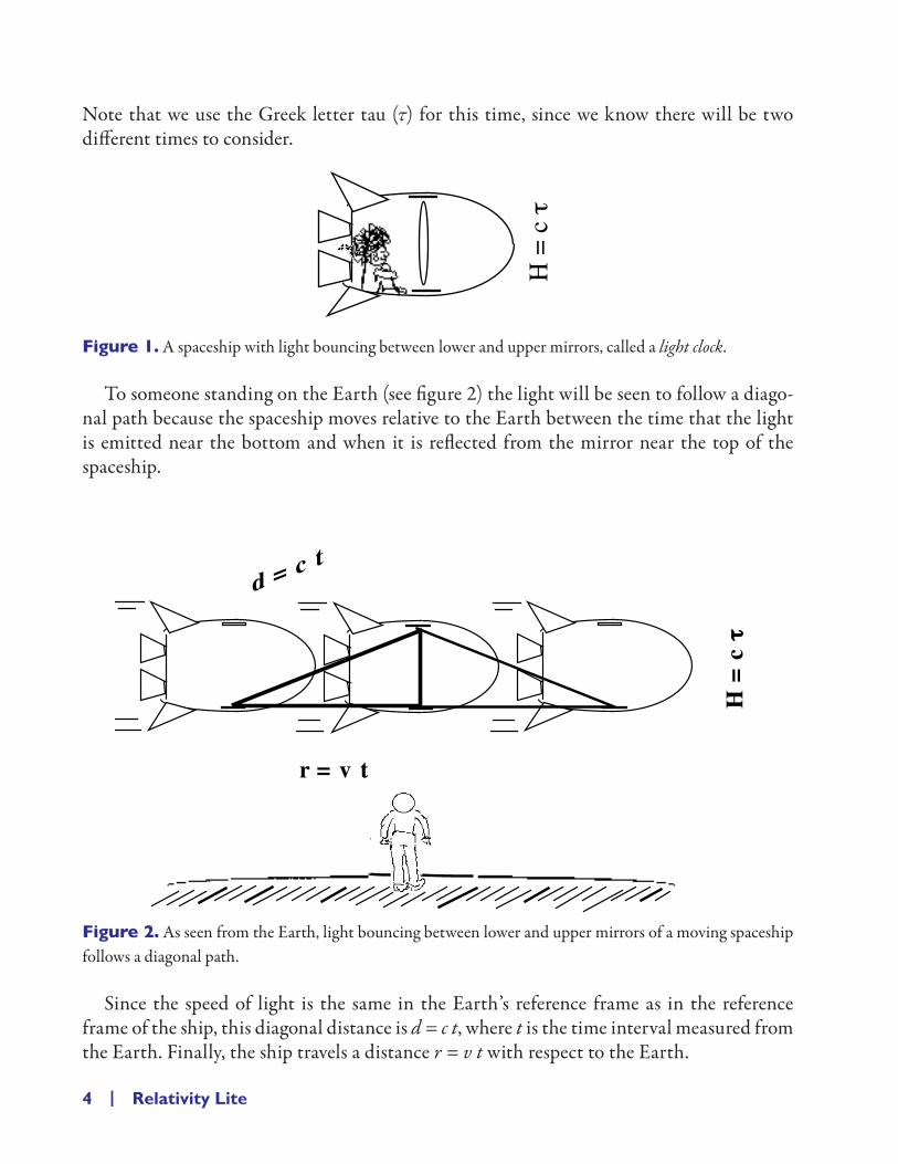
To someone sitting in the ship, the distance the beam must travel is simply the height H of the ship. The distance is the velocity c times the time of travel τ between bounces as measured in the ship or
H = c τ.
4 | Relativity Lite
Note that we use the Greek letter tau (τ) for this time, since we know there will be two different times to consider.
H =
c τ
Figure 1. A spaceship with light bouncing between lower and upper mirrors, called a light clock.
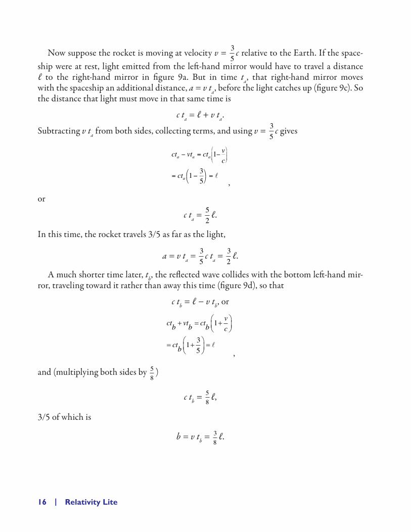
To someone standing on the Earth (see figure 2) the light will be seen to follow a diago-nal path because the spaceship moves relative to the Earth between the time that the light is emitted near the bottom and when it is reflected from the mirror near the top of the spaceship.
r = v tH
= c
ττ τττ
d = c t
Figure 2. As seen from the Earth, light bouncing between lower and upper mirrors of a moving spaceship follows a diagonal path.
Since the speed of light is the same in the Earth’s reference frame as in the reference frame of the ship, this diagonal distance is d = c t, where t is the time interval measured from the Earth. Finally, the ship travels a distance r = v t with respect to the Earth.

To c or Not to c | 5
It is clear from figure 2 that the hypotenuse d of the triangle is longer than the vertical leg H. Then since the speed of light c is the same for both the hypotenuse and the verti-cal leg, t must be larger than τ. But the hypotenuse of any right triangle you can draw is always longer than each leg or is equal to the length of one leg if the length of the other is zero. (Draw several examples to prove this to yourself.) This means that t is always larger than τ for nonzero v. We call this minimum time value τ proper time. It is simply the time measured in any frame in which the two events are measured at the same place, such as the emission and the return points of the bouncing beam of light, or two clicks of a clock. The coordinate time interval t is measured in a frame of reference moving at velocity v relative to the frame in which the clock is stationary. (If we want to be precise, τ in figure 1 is actually half of the proper- time interval for a round trip 2 τ. Likewise, in figure 2, t is half of the corresponding coordinate time 2 t.)
HOW DOES THIS RELATE TO ME?We say that the coordinate time is dilated. What exactly does that mean? It means that if your twin sister drives a fast car while you walk everywhere, she will live longer than you do— her lifetime will be dilated relative to yours! By how much?
We could find how much larger t is than τ by using the Pythagorean theorem and some algebra* but there is a simple way to get the time- dilation factor by drawing the spaceship picture carefully, with v properly proportional to c as demonstrated in figure 3:
1. Start with a square that is 10 cm on each side (the bottom side of which represents the distance light travels in the coordinate frame of reference).
2. Now express the velocity of the spaceship as a fraction of the speed of light and draw a rectangle that is that same fraction of 10 cm wide and is the full 10 cm high.† Suppose v is 3
56
10= of the speed of light (111,600 miles/second); then the width of
the rectangle is 6 cm, shown as red as in figure 3.
* Suppose vc
= 35
; then the ratio of the flight path (in the Earth’s frame of reference) to the light path is also 35
. Let us use
3 cm and 5 cm, respectively. We can use the Pythagorean theorem to relate the two times, τ and t:
(flight path)2 + (vertical light path)2 = (diagonal light path),2
or (vertical light path)2 = (diagonal light path)2 − (flight path)2 = 25 cm2 − 9 cm2 = 16 cm2. This means that the vertical
light path is 4 cm. Then t/τ = 54
or 1.25.
† Suppose the speed is v = 111,600 miles/second. Then the fraction vc
= 111600186000
miles secondmiles second
//
= 0.6. The width of the rectan-
gle would then be 0.6 × 10 cm = 6 cm.

6 | Relativity Lite
3. Now trace the square onto a thin sheet of paper (or cut out a square of this size) androtate the square around the lower left- hand corner until the lower right- hand cor-ner of the square just touches the right- hand edge of the rectangle, approximatedby the sequence of three rotated green squares shown in figure 3.
c τ
c tv t
c t
Figure 3. The sequence of fours steps described in the text in full. The red rectangle has a width that represents the distance the spaceship travels (6 cm) in an extremely short time compared to the distance light
travels, the width of the full 10 cm square, if v is 35
610
= of the speed of light. If v had equaled c, these widths
would have been equal. The sequence of three rotated green squares are stop- motion animation versions of the smooth rotation of the square by the reader. The blue arrows indicate the height measurement asked of the reader.
4. Tape the square in place and measure the distance from the lower right- hand cor-ner of the rotated square to the lower right- hand corner of the rectangle. For thepresent example, this length is 8 cm, shown as blue in figure 3. Divide 10 cm bythis length to get the value of the time- dilation factor. In the present example, this
ratio is 54
, or 1.25.

To c or Not to c | 7
If your twin rides around in a spaceship at 111,600 miles/second for 40 years, 50 years will have passed for you when she returns! That may seem strange to you, but she is travel-ing at about 400 trillion miles/hour, something not exactly within your normal range of experience.
Suppose your twin slows way down, to 1/10th of the speed of light (see figure 4). Her speed is v = 0.1 c, so the width of the rectangle is 1/10 of 10 cm or 1 cm.
v tc t
c τc t
Figure 4. The sequence of fours steps for v = 0.1 c.
As you rotate the rectangle, you notice that c t = 10 cm is not much longer than c τ = 9.95 cm. This simply shows that the dilation of coordinate time (1.01 in this case) becomes unnoticeable at velocities that are small compared to c.
So suppose your twin drives around at 70 miles/hour or 0.019 miles/second (figure 5). That is v = c/1000000 so the width of the rectangle should be 10 cm/1000000, or 80,000

8 | Relativity Lite
times thinner than the narrowest line this printer can draw at 300 dots per inch. Even if you could draw it, you cannot see any difference between c t and c τ, so no time dilation comes into our everyday experience.
v tc t
c τc t
Figure 5. The sequence of fours steps for v = 70 miles/hour.
RELATIVITY BITES
This is not to say that time dilation does not affect our lives. The Earth is bombarded by cosmic rays that produce showers of particles called muons in the upper atmosphere. Half of a given group of muons decays within two- millionths of a second (two microseconds) when they are at rest. That is, they have a proper half- life of two microseconds. After another two microseconds, half of those remaining decay, leaving one- fourth, and so on.

To c or Not to c | 9
If there were no relativistic time dilation, most would decay as they travel through the depth of the atmosphere before crashing through your skull. We will show later that on average, the muons are traveling to the Earth’s surface at v = 0.9986 c. At this speed, it would take them 16 microseconds to travel through the atmosphere from the height they are produced, about 3 miles,* or about 8 half- lives.† It turns out that 18 muons are created
each second over an area the width of our bodies. After 8 half- lives, 128 × 18 = 0.07 muons
per second should be left to crash through our bodies. Table 1 shows a progression of halv-ing the prior number, with some rounding.
Table 1. The half- life progression for 18 muons at the start.
Time Muons left
0 µs 182 µs 94 µs 4 or so6 µs 28 µs 1
10 µs 0.512 µs 0.314 µs 0.1516 µs 0.07
But relativity changes all this. To find the time- dilation factor for this speed, we find that we only need to rotate the square slightly to get the lower right- hand corner of the square to just touch the right- hand edge of the rectangle (see figure 6).
* A. W. Wolfendale, Cosmic Rays at Ground Level (Institute of Physics, London, 1973), p. 174– 75.
† t = d
c.9986 =
39986 186000
milesmiles second. /×
= 3
1 86. ×
101000000
seconds = 16 microseconds.

10 | Relativity Lite
c tc τc t
v tc t
Figure 6. The sequence of fours steps for v = 0.9986 c.
In this case, c t = 10 cm is much longer than c τ = 0.52 cm. The coordinate time is extremely dilated by a factor of 19. So thanks to relativistic time dilation you measure a muon’s half- life at 19 times its proper half- life, or 38 microseconds. This is about twice the time it takes for the muons to travel through the atmosphere. That is, roughly 1/4 of them will decay, and 13 muons make it through each second* to crash through your skull and increase your cancer rate. The typical yearly dose of radiation due to these muons is 400 µsv (microsievert),† 6 times higher than a typical yearly dose of radiation due to diag-nostic X- rays, 70 µsv.‡ If there were no relativistic time dilation, the yearly radiation dosage
* National Council on Radiation Protection and Measurements, Report No. 94, Exposure of the Population in the United States and Canada from Natural Background Radiation (NCRP, Bethesda, MD, 1987), p. 12, has a rate of 0.00190 muons per cm2 per second at the surface. I obtained 13 muons per second by modeling a person by a cylinder with a radius of 15 cm.
† Alan Martin and Samuel A. Harbison, An Introduction to Radiation Protection (Chapman & Hall, New York, 1979), p. 53, gives 500 µsv for all types of cosmic radiation, of which muons make up 80%, according to the National Council on Radiation Protection and Measurements, Report No. 94, Exposure of the Population in the United States and Canada from Natural Background Radiation (NCRP, Bethesda, MD, 1987), p. 12.
‡ Alan Martin and Samuel A. Harbison, An Introduction to Radiation Protection (Chapman & Hall, New York, 1979), p. 57.

To c or Not to c | 11
from muon exposure would be only 2 µsv. (For perspective, if I were to ask you to give me $2, the chances are pretty good you might do so. But if I asked you to give— not lend— me $400, the chances you might do so would be pretty slim.) Relativistic effects are not a minor factor in our lives at all!
Just so that you do not get the idea that the real- world consequences of relativity are all negative, consider that evolution works by taking advantage of mutations. Theistic philos-ophers struggle with the question of why there are disease and evil in the world. In his last book, And God Laughed When the Birds Came Forth from the Dinosaurs, my father asked the question this way:
[W]hy does God allow such mutation, which, from the higher standpoint of the personal value that it destroys, must be classified as an “evil”? The answer that seems reasonable is to affirm that such mutation . . . is the risk God must run in creating or bringing forth a finite world of freely developing process. The over- all rationality of such possibility seems borne out by the thoughtful conclusions of genetical science itself. The geneticists Dunn and Dobzhansky write:
Harmful mutations and hereditary diseases are thus the price which the species pays for the plasticity which makes continued evolution possible.*
[T]he above quotation contains the idea of the neutrality of mutations as a necessary principle of . . . physical process. The mutation of the genes makes the survival of life possible in the long run in any environment, or amid environmental changes, within, of course, upper and lower limits of temperature and other absolute environmental boundaries for life. In theistic faith, and from the standpoint of values, this “neutrality” of mutation would itself seem purposive, since its effect is that life does survive. To theistic faith, the immanent rationale of mutation is that life shall survive.†
He also writes,
[A] modern teleological‡ view of evolution would cite mutation itself— the capacity of life at the very deepest level of process to adjust or adapt itself— as significant evidence of an ulti-mate spiritual meaning, design, or purpose within our world’s evolutionary development. The spiritual meaning inheres in this “free capacity,” which makes possible the manifold growth
* L. C. Dunn and Th. Dobzhansky, Heredity, Race, and Society, A Mentor Book (New American Library, New York, 1946/1952), p. 81.
† G. Douglas Straton, And God Laughed When the Birds Came Forth from the Dinosaurs: Essays on the Idea and Knowledge of God (1995 ms.), Chap. 6, p. 163.
‡ Teleology is the study of cosmic design.

12 | Relativity Lite
and integration of life in many experimental directions, instanced by all the past and present organic forms.*
Clearly, if relativity were not working, evolution would have proceeded at a pace that is between 5 and 256 times slower (28).† The Earth would have had to wait 18 to 900 billion years for intelligent life to form (instead of 3.5 billion years)— much longer than the Sun’s 10- billion- year lifetime!
Put another way, the person attempting to write this book today would likely be a mess of green slime had relativity not offered us its gifts.
THERE ARE COPS, YOU KNOW!What about people traveling at super high speeds, such as v = 0.9986 c in figure 6? Suppose your twin left Earth when you were 20 years of age, traveled for 10 years at v = 0.9986 c, and then returned to Earth to tell you about her trip. Tough luck; you would have died of old age a century before she returned! You were both 20 when she left. She is 30 years old (20 + 10) when she returns (both her clock and her body agree with this assertion), but you would be 210 years old (20 + 10 × 19) had you lived.
As we increase the speed from this point, we will find that we reach a limit in our ability to graph. But this limit expresses a reality of nature. As the velocity v of a rocket approaches that of the speed of light c, the right- hand side of the rectangle really does approach the right side of the 10 cm square in figure 6. The limit as v goes to c is that the rectangle goes to a square. Then we have to move the square not at all to get its lower right- hand corner to touch the right side of the rectangle- which- is- a- square. That is, c τ = 0 cm.
A finite coordinate time period in a rocket moving at velocity v = c relative to the Earth corresponds to zero proper time. What does that mean? If we divide 10 cm by 0 cm we get an infinite time- dilation factor.‡
We actually never run into this infinite limit because it is impossible to exert sufficient force on the rocket to get it moving at the speed c. The reason is that whatever force is exerted on the rocket to increase its velocity is spread out over a longer and longer period of Earth coordinate time as v approaches c. We would have to wait an infinite amount of Earth coordinate time to see the rocket reach the speed of light.
* G. Douglas Straton, And God Laughed When the Birds Came Forth from the Dinosaurs: Essays on the Idea and Knowledge of God (1995 ms.), Chap. 5, p. 115.
† The maximal value is assuming that the other 100 µsv of cosmic radiation noted in Alan Martin and Samuel A. Harbison’s An Introduction to Radiation Protection (Chapman & Hall, New York, 1979), p. 53, would have a similar reduction in the absence of relativity; the minimal value assumes that there would be no such reduction.
‡ To see this consider the following pattern: On your calculator divide 10 by 10 to get 1; 10/1 = 10; 10/0.1 = 100; 10/0.01 = 1,000; 10/0.001 = 10,000; 10/0.0001 = 100,000; 10/0.00001 = 1,000,000; and so on. As you divide 10 by smaller and smaller numbers, you get a result that is bigger and bigger. Infinity is the limit of this sequence.

To c or Not to c | 13
To see how this works, imagine a spaceship powered by small nuclear bombs that are dropped through a small hole in a radiation shield attached to the passenger cabin. When a bomb explodes, half of the exploded material and associated photons push against the radiation shield, shoving the rocket faster in its direction of travel. As the rocket’s veloc-ity increases, the time dilation increases on Earth, which the passengers have left behind. As the rocket crew steadily drops and explodes bombs (at a steady proper- time interval), there are longer and longer time intervals between when Earth folk see the photons from the explosions arrive. In fact, as the people on Earth see the rocket’s speed approach the speed of light, they have to wait through an infinite time interval for the explosion that would have just pushed the rocket past the limit. Thus, the rocket never reaches the speed of light relative to the Earth. One might rephrase the classic Western koan as “What happens when an irresistible force meets an interminable stasis?”
Some readers will note that many science popularizers and introductory physics teachers used to invoke the idea that
[t]he faster a particle is pushed, the more its mass increases, thereby resulting in less and less response to the accelerating force. . . . [A]s v approaches c, m approaches infinity! [To push a particle] to the speed of light . . . would require an infinite force, which is clearly impossible.*
Let me caution you that research physicists rely heavily upon the fact† that the mass of a particle is the same in all frames of references; it is an invariant quantity.‡
See, for instance, the caption of figure 4 in the paper publishing the discovery of the Higgs boson,§ reproduced below, that begins with the explicit acknowledgment of the “[i]nvariant mass distribution,” while the simpler and equivalent “mass” is also used through-out, such as in the section G, following that figure: “The measured Higgs boson mass [is] 125.98 ± 0.50 GeV. . . .” The (invariant) mass of an object is sometimes referred to in older texts as the “rest mass.”
* Paul G. Hewitt, Conceptual Physics, 6th ed. (Scott, Foresman & Co., Boston, 1989), p. 662.† For a complete history of this, see Lev. B. Okun, Phys. Today 42, 31– 36 (June 1989).‡ See, for instance, the standard textbook by John D. Jackson, Classical Electrodynamics (John Wiley & Sons, New York,
1975), p. 531, eq. (11.54).§ G. Aad et al. (ATLAS Collaboration), Phys. Rev. D 90, 052004 (2014).

14 | Relativity Lite
Figure 7. Invariant mass distribution in the H → γγ analysis for data (7 TeV and 8 TeV samples combined), showing weighted data points with errors, and the result of the simultaneous fit to all categories. The fitted signal plus background is shown, along with the background- only component of this fit. The different categories are summed together with a weight given by the s/b ratio in each category. The bottom plot shows the difference between the summed weights and the background component of the fit.
Figure 4 of G. Aad et al. (ATLAS Collaboration), Phys. Rev. D 90, 052004, reproduced under the terms of the Creative Commons Attribution 3.0 License.
The idea that mass increases with velocity was introduced by Hendrick Lorentz* in 1899 so that he could use the low- speed expression for momentum, m v, for relativistically high veloci-ties. When Einstein introduced relativity six years later, the idea of mass increasing with velocity became unnecessary, but unfortunately, it has retained a very long life. This puts you, the reader, in the nasty position of having to decide between two “authorities.” Since the explanation for the upper limit on rocket speeds given on the previous page does not need to mention mass, changing or otherwise, Occam’s razor† would dictate that we choose it over an explanation that includes the idea of varying mass. I would recommend that you discard the latter idea as outdated. After
* H. Lorentz, Proc. R. Acad. Sci. Amsterdam 1, 247 (1899); 6, 809 (1904).† William of Occam (c. 1280) said that when there are several explanations of a phenomenon, the simplest is most likely to
be correct.

To c or Not to c | 15
all, the downside of using a convenient, though incorrect, model to make predictions is revealed well in the story of the Ptolemaic vs. Copernican models of the Solar System.
A SHORT TALESo everything you believe about time has just gotten blown out the window. About now, I would expect you to be wondering if space gets messed with too. It does.
Unfortunately, the pictures below show this only with the aid of a series of length compar-isons. In my experience, those who are a bit wigged out by math may put up with a single such relation here and there, but a series of about eight length comparisons that build up to the answer may well lead to frustration. So let me simply give you the result here and you can just skim over the notes below as if they were written in Portuguese, from which a recognizable word or two might pop out if you know a bit of Spanish or French. If you would like to bypass the compari-sons entirely, read the following paragraph and then just jump to the words Skip to here.
The length ℓ of the rocket measured by Earth is contracted by the same factor, relative to the proper length L, as the time t measured by Earth is dilated relative to proper time τ. Since we keep on finding this “factor,” we had better give it a name. It is always represented by the
Greek letter for g, gamma, which is written γ. That is, t = γ τ, and ℓ = Lγ .
Here are the details. Consider our spaceship at rest, with an additional pair of mirrors set at the same distance horizontally as the original ones were set vertically (see figure 8). Then if a light wave is emitted from the lower left- hand corner of the set of mirrors, it will travel outward in concentric rings, strike the top and right- hand mirrors simultaneously, and be reflected back to the emission point. The total distance traveled in this proper- time interval is
2 L = c τ.
Figure 8. A spaceship with vertical and horizontal light clocks.
16 | Relativity Lite
Now suppose the rocket is moving at velocity v = 35
c relative to the Earth. If the space-ship were at rest, light emitted from the left- hand mirror would have to travel a distance ℓ to the right- hand mirror in figure 9a. But in time ta, that right- hand mirror moves with the spaceship an additional distance, a = v ta, before the light catches up (figure 9c). So the distance that light must move in that same time is
c ta = ℓ + v ta.
Subtracting v ta from both sides, collecting terms, and using v = 35
c gives
ct vt ct vc
ct
a a a
a
− = −
= −⎛⎝
⎞⎠
=
⎛
⎝
⎜⎜
⎞
⎠
⎟⎟1
1 35
,
or
c ta = 52
ℓ.
In this time, the rocket travels 3/5 as far as the light,
a = v ta = 35
c ta = 32
ℓ.
A much shorter time later, tb, the reflected wave collides with the bottom left- hand mir-ror, traveling toward it rather than away this time (figure 9d), so that
c tb = ℓ − v tb, or
ctb vtb ctbvc
ctb
� � ����
���
� ����
��� �
1
1 35
,
and (multiplying both sides by 58
)
c tb = 58
ℓ,
3/5 of which is
b = v tb = 38
ℓ.

Figure 9a.
Figure 9b.
Figure 9c.
Figure 9d.
a
L
r
b

18 | Relativity Lite
Then the total distance the rocket travels for the emission and reflection is the sum of these, r vt a b= = + = × + = ×
32
44
38
58
3 , which is again 35
of the distance the light travels in the
same time, ct = × + = ×52
44
58
5 58
. We found from our time- dilation calculation in figure 2 that if one leg is 3 units long when the hypotenuse is 5 units long, then the other leg has to be 4 units long. This is the case in the two expressions above for the leg and hypotenuse, where the unit of measure is 5
8 . So cτ = ×4 5
8 .
But from figure 8, we see that c τ = 2 L. Comparing these two expressions shows that
ℓ = 85
× 24L = 4
5 L.
(Skip to here.) Comparing this to the time- dilation expression we obtained from figure 3, t = 5
4 τ shows that the length ℓ of the rocket measured by Earth is contracted, relative to
the proper length L, by the same factor γ = 54
, as the time t measured by Earth is dilated
relative to proper time τ. That is t = γ τ and ℓ = Lγ
.
This compensation between time dilation and length contraction is necessary for real-ity to be whole. Einstein’s second postulate of relativity was that no experiment you could perform would tell you whether it was your frame of reference that was moving or someone else’s (alternatively stated, motion is relative, or there is no preferred frame of reference).
Consider our example of the time dilation of muons created in the Earth’s atmosphere. These muons are free to think they are at rest and it is the Earth that is moving toward them. They see the surface of the Earth traveling toward them at v = 0.9986 c just after they are produced.
At this speed, it would take the Earth’s 3 miles of atmosphere 16 microseconds to pass by them before the surface crashes into them. As before, this is about 8 proper half- lives. If there were no relativistic length contraction, most would decay before they saw your head approaching as you stood on the surface of the Earth. But because of relativity, the muons see the Earth’s atmosphere contracted to only 1/6 of a mile.* The time it takes the Earth’s surface to hit them is then 0.8 microseconds, or about half of the muon half- life.† Again, we get the result that roughly 1/4 of the muons decay, leaving 13 muons getting hit by your head each second before their lives are over. Without length contraction, the physical reality of your cancer risk would depend on which frame of reference does the calculation. That would violate Einstein’s principle of relativity.
* ℓ = 319
miles = 0.158 miles.
† t =
.9986 c = 0 1589986 186000
.. /
milesmiles second×
= 0 158186.
. × 11000000
second = 0.854 microseconds.
Mixmaster Universe | 19
CHAPTER 2
Mixmaster UniverseShall we now go on to prove Einstein’s famous mass- energy relationship? May I suggest that you first put on some music to take you elsewhere for a while? If you have not sampled much in the way of 1960s jazz, let me suggest Charles Lloyd’s “Forest Flower” (from the album of the same name, recorded live at the Monterey Jazz Festival in 1966). If you play both the Sunrise and Sunset portions, your brain may then be ready to come on back online.
To prove Einstein’s famous mass- energy relationship most clearly, it helps to return to our graphic calculator from the previous chapter and figure out why it works so well for low- ish speeds.
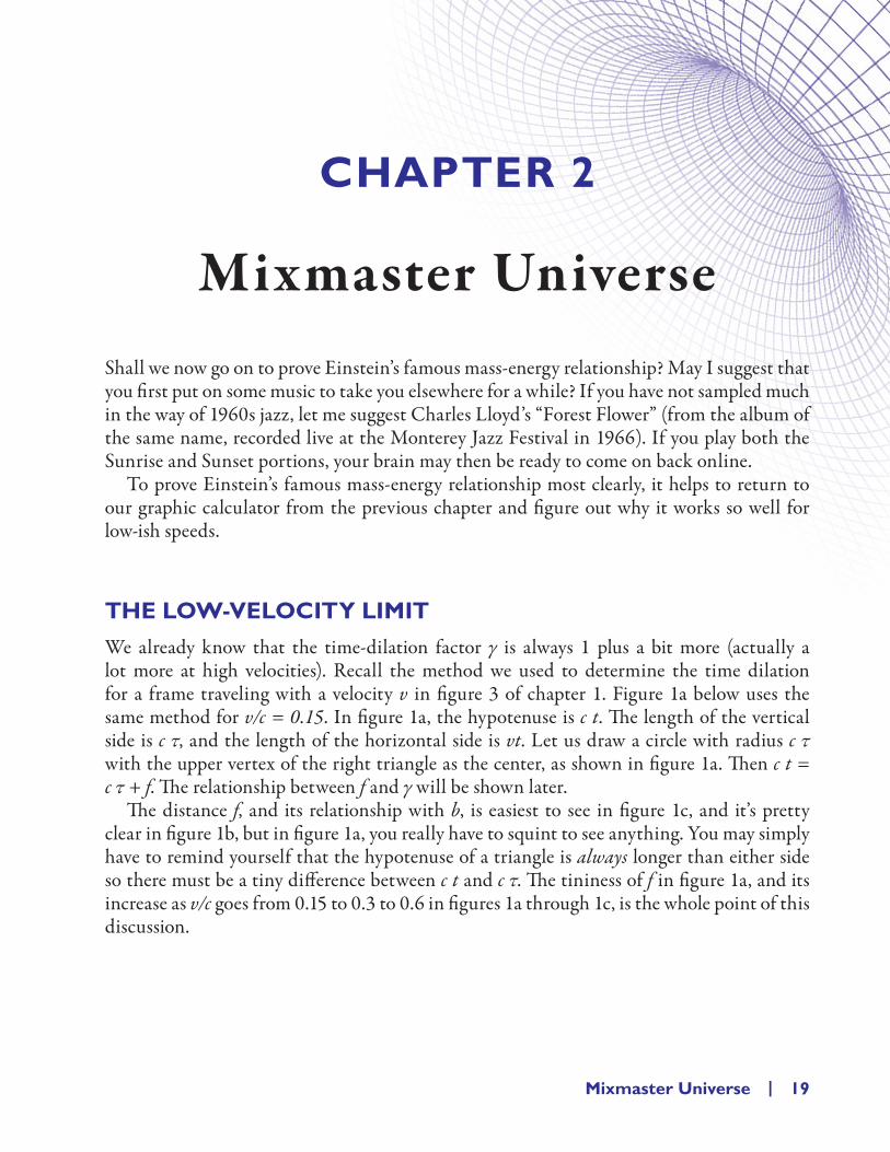
THE LOW- VELOCITY LIMITWe already know that the time- dilation factor γ is always 1 plus a bit more (actually a lot more at high velocities). Recall the method we used to determine the time dilation for a frame traveling with a velocity v in figure 3 of chapter 1. Figure 1a below uses the same method for v/c = 0.15. In figure 1a, the hypotenuse is c t. The length of the vertical side is c τ, and the length of the horizontal side is vt. Let us draw a circle with radius c τ with the upper vertex of the right triangle as the center, as shown in figure 1a. Then c t = c τ + f. The relationship between f and γ will be shown later.
The distance f, and its relationship with b, is easiest to see in figure 1c, and it’s pretty clear in figure 1b, but in figure 1a, you really have to squint to see anything. You may simply have to remind yourself that the hypotenuse of a triangle is always longer than either side so there must be a tiny difference between c t and c τ. The tininess of f in figure 1a, and its increase as v/c goes from 0.15 to 0.3 to 0.6 in figures 1a through 1c, is the whole point of this discussion.

c τ
vtc t
c τc t
θ
bf
Figure 1a. Relativistic relationships for v/c = 0.15.
Figure 1b. Relativistic relationships for v/c = 0.3.

Mixmaster Universe | 21
Figure 1c. Relativistic relationships for v/c = 0.6.
If we overlay the 9.89 cm c τ line in figure 1a on the 10 cm hypotenuse c t, the excess is f = 0.11 cm for v/c = 0.15. As we double the speed to v/c = 0.3, and overlay the 9.54 cm c τ line in figure 1b on the 10 cm hypotenuse c t, the excess is f = 0.46 cm. This is a factor of 4.2 times larger than the previous value, or slightly more than the square of 2, the factor by which we increased the velocity. To see if f actually increases with the square of the veloc-ity, let us double it again to v/c = 0.6. If we overlay the 8 cm c τ line in figure 1c on the 10 cm hypotenuse c t, the excess is f = 2 cm. This is a factor of 4.3 times larger than the pre-vious value, or slightly more than the square of 2— again, the factor by which we increased the velocity. This “slightly more” than the square of 2 also has increased but less quickly as the velocity changed.
We can relate this excess f as the second term on the right- hand side of
γ γ≅ +1 12
2
2
vc ,
where the “slightly more” that keeps cropping up is expressed by the factor γ, which we know is “slightly more” than 1. Those willing to put up with several steps of substitutions can look in this footnote* to see the veracity of this relation.
* To see that γ is 1 plus something proportional to v2/c2 plus a slight correction, we can use geometry or the Pythagorean theorem. If you are more comfortable with the latter, skip to the third paragraph of this footnote. Look at figures 1b and 1c, where one can see that I have also drawn in a line perpendicular to the hypotenuse to form a miniature triangle that has

22 | Relativity Lite
Please note that this relation is not an “equation,” since it involves an approximation symbol and has γ, on both the left and right sides. It is an iterative relation that is probably best read as a recipe:
Take a rough value for γ and multiply it by 12
2
2
vc .
Add 1 to the result.Stir for 15 seconds.Yield: 1 serving of a slightly better version of γ.
We noticed in the last chapter that γ seems to be “1 plus a bit more” for a wide range of velocities. Let us take 1 as our “rough value for γ,” and call it γ0. Our recipe serves up of a slightly better version of γ, which we find to be
γ γ1
2
2 0
2
2
2
21 12
1 12
1 1 12
≡ + = + = +vc
vc
vc .
We could keep on going in this fashion and find a third term that will depend on the fourth power of the velocity.
Those of you who are a bit queasy about math can just plug your ears and say “LA LA LA” out loud while I write that one can apply the Pythagorean theorem to figure 1 and discover the exact expression for γ to be
γτ
= ≡
−
tvc
1
12
2
,
which involves a square inside a dreaded square root at the bottom of the sea, so it is not as convenient as is our γ1, but you can get numbers out of your calculator for high speeds
exactly the same shape as the triangle with hypotenuse c t, long side c τ, and short side v t, but rotated so that the miniature triangle’s hypotenuse is facing downward. You may remember the term similar triangles from ninth grade geometry: two such triangles have ratios of sides to each other (and, thus, angles) that are the same. The miniature triangle has hypotenuse
v t and short side b so the ratios of these two sides for the miniature and big triangle are equal, bvt
vtct
= , or bv tc
=2
. Finally, we note that the f in figures 1a, 1b, and 1c is in each case about 1/2 b, perhaps with a slight correction unnoticeable to the eye.
Above, when we said we would “overlay the 9.54 cm c τ line in figure 1b on the 10 cm hypotenuse c t,” and saw that “the excess is f = 0.46 cm,” we were simply taking the ratio of c t to c τ, which we know is the time- dilation factor γ. Putting these words into ratios,
γτ
ττ τ τ τ
≡ =+
= + ≅ + = + = +ctc
c fc
fc
bc
vc
t vc
1 1 12
1 12
1 12
2
2
2
2 γγ .So our guess that f is dependent on the square of the velocity was a good one. If you more or less followed this geometrical method, skip the following.
One could instead use the Pythagorean theorem: We square the hypotenuse c t = c τ + f of the original, big triangle (and expand this square). We then equate it to the sum of the squares of the other two sides: f c f fc c vt c+( ) = + + ( ) = ( ) + ( )τ τ τ τ2 2 2 2 22 . Since f is small, its square will be much smaller and can be ignored in the above. Canceling the factor of cτ( )2 that appears
on both sides and dividing both sides by 2 2cτ( ) gives fc
vc
tτ τ
≅12
2
2 , where we have kept one factor of t/τ and set the other
one to reproduce the approximation that f is half of b, which gives the fifth version of the equation for γ in the previous paragraph.

Mixmaster Universe | 23
where our γ1 loses accuracy.* This becomes apparent as we calculate γ1 and γ for various velocities:
Table 2. Approximate γ1 and exact values (truncated to five decimal places) for the time- dilation factor γ
τ=
t .
vc
vc
2
2
12
2
2
vc
γ 1
2
21 12
≅ +vc
γ ≡
−
1
12
2vc
0.1 0.01 0.005 1.005 1.005030.2 0.04 0.02 1.02 1.020620.3 0.09 0.045 1.045 1.048280.4 0.16 0.08 1.08 1.091090.5 0.25 0.125 1.125 1.154700.6 0.36 0.18 1.18 1.25
It seems that γ1 works pretty well for velocities below half the speed of light.Now would be a good time to go put on some obnoxiously loud rock music to release any
tension you may have over going through this derivation. May I suggest Led Zeppelin’s The Ocean (Live at Madison Square Garden, 1973)? When you have done that, come on back.
INTO THE MIXNow look closely at figure 8 of chapter 1. The light is reflected from the right- hand mirror at the same time that the light is reflected from the top mirror. These events are simultaneous in the rest frame of the rocket. But in figures 9b and 9c in chapter 1, the light is reflected off the top mirror before it is reflected off the right- hand mirror, not simultaneously! (But the return sequence to the lower left- hand corner is simultaneous for both frames of reference.) The sequence of events in different frames of reference moving relative to each other is not necessarily the same when you live in Einstein’s universe.
The time interval between two events I measure on my clock depends not only on the time interval you measure on your clock (time dilation) but also on where you are standing relative to the other event in your frame of reference. In other words, my time depends
* Did you ever wonder how your calculator actually finds this beast? It uses a series of approximations:
��
� � ��
��
�
�� � � ��
��
��� �
����
��� ����
����
t vc
vc
v1 1 12
12
32
2
2
2
12 2
2
2
cc2
2�
��
�
�� � , and so on, which confirms that our “‘slightly more’ than [ f ]” above will
depend on the fourth power of the velocity and several of higher powers to get 10- digit accuracy.

24 | Relativity Lite
on your space too.* In our rocket moving at velocity v = 35 c, a watch on our astronaut in
figure 1 of chapter 1 would read a time tw w= 54
τ to us on Earth, while a clock sitting a dis-tance x away on the floor of the spaceship— that our twin asserts is perfectly synchronized with her watch in her frame of reference— would read to us
txc
vc
xcc c w= =γ τ τ−
−
54
35 ,
a different time, unless the clock is just under the watch on her right hand, at x = 0.Equally as strange, my measurement of space x' (this prime is my means to distinguish my
space from yours) in the direction of your motion x likewise depends on your time:
x x v x c y y z z' ( ) , , '= − = −
=γ τ τ54
35
'= ,
but perpendicular distances are unaffected. (For this reason, angles that extend into the x' direction will be affected.)
Not only does relativity force us to give up “absolute time”; it also forces us to give up the idea that “space” (a three- dimensional world that we can group together as {width, length, and height}— or, if you prefer, {north, west, and up}) and “time” (a one- dimensional marker of {duration}) are entirely separate actualities. We have to begin to perceive the universe as a four- dimensional spacetime. To use a word analogy for the math, a spacetime event that you measure as {duration, width, length, and height} may be perceived by someone else moving relative to you as {duration coupled to length, width, length coupled to duration, and height}.
Just as space and time constitute a four- dimensional entity of the universe {c t, north, west, up}, so do other common quantities like momentum and energy. I had a fairly petite woman named Catherine Wong in my 2013 Freshman Inquiry class who plays rugby (figure 2). Suppose you are on the field watching her as she barrels into you heading north. What happens? (You get knocked a few feet north.) What else happens? (Some of her motional energy [kinetic energy, or KE] gets deposited into your body, which you experience as pain in your stomach.) Suppose she instead barrels into you heading west while you were still looking south. What happens? (You get knocked few feet west.) What else? (Some of her KE is deposited into your body, which you experience as pain in your side.) Suppose she instead tosses the ball high above your head and you reach up to catch it. What happens? (Your hands recoil a few inches downward.) What else happens? (Some of the ball’s KE gets deposited into your body, which you experience as stinging palms.)
* ′ = −( )x x vtγ and ′ = −( )t t vx cγ 2 for motion in the x direction.

Mixmaster Universe | 25
Figure 2. Catherine Wong playing rugby (used by permission).
These are each different experiences of our three- dimensional world of momentum that have in common the pain characteristic of the deposition of energy into your body, the final entry in this gang of four, {energy/c, northward momentum, westward momentum, upward momentum}. Just as we usually write the spacetime four- dimensional vector as abbreviated symbols {c t, x, y, z}, so too the energy- momentum four- dimensional vector is written in abbreviated symbols {E/c, px, py, pz}. Why the momentum is px, and not mx, is historical and avoids confusion with the symbol m used for mass.
I do not know Catherine’s weight, so let us just pin it at a nice round number like 100 pounds. Suppose instead of her, a 200- pound player going at the same speed runs into you. How will the pain compare? (It will be worse.) As you might expect, smaller people can often get going much faster than larger people, so imagine now that Catherine is running twice as fast as the 200- pound player. Who is going to hurt you more? That is right, she will. Even if she is only going 50% faster, she will wham you worse and cause more pain. This is a life lesson in respect that is important to learn.
It turns out that a player who runs into you at twice the speed of a second one will hurt you four times as much, but an equal- speed player who is twice as heavy as the first one will hurt you only twice as much. That can be quantified by the relation
KE mv=12
2 .*
* You can verify that a ball falling 5 meters in 1 second will have a velocity of 10 m/s. Its kinetic energy is equal to the grav-
itational potential energy it had before falling, KE m m mgh= ( ) = ( )( ) =12
10 10 52 m/s m/s/s m , where g is the acceleration of gravity
(10 m/s/s) and h is 5 m.

26 | Relativity Lite
IS NOTHING SACRED?The triangle in figure 2 of chapter 1 is a useful way to comprehend a four- dimensional re-ality on a two- dimensional sheet of paper. The hypotenuse is the time part (c is a constant so c t really just tells us about t), and the horizontal leg, labeled v t, is the space part, since it has to do with the motion of the rocket through space. In special relativity, we can often ignore the fact that space really has three dimensions, because the rocket really only moves along a one- dimensional line.* The third side of the triangle, labeled c τ, represents proper time, an example of a relativistic invariant, something that each of us measures as being the same in our own reference frame. The speed of light c is another example of a relativistic invariant. No matter who measures the half- life of a muon that is at rest relative to their rocket ship, they all get the same value. So although time is relative between moving frames, it is not unknown. We will always agree on what you will measure for t, the lifetime of muons on my rocket, if I am flying past you at velocity v, even though t is not equal to my τ.
One beautiful element of order in the universe is that it has patterns we can perceive. Suppose we take the triangle in figure 2 in chapter 1 and multiply the length of each side by the rocket’s mass (abbreviated as m) and by c and then divide each side of it by proper time τ.†
Then the new figure looks like figure 3 below.
c t × m c / τ
= E
r = v t
d = c t
H =
c τ
v t × m c / τ = momentum × c
c τ
× m
c /
τ =
m c
2
Figure 3. The triangle of figure 2 in chapter 1 multiplied on each side of by the rocket’s mass m and by c and then divided on each side by proper time τ.
* If the rocket starts to curve, it experiences acceleration (like you feel when your car turns a corner), and we must then turn to Einstein’s general theory of relativity, as we do in the next chapter.
† Some readers will have noted that such a procedure is only mathematically valid if mc τ has the same value in all frames of reference. We know that c is the same in all frames. We defined proper time τ as an invariant quantity, the time interval of two events that occur at the same place (at rest) in any frame of reference. As discussed on page 13, mass m is also an invariant quantity, the same in all frames of reference.

Mixmaster Universe | 27
The new triangle has the same shape as the old one. They are called similar triangles, having the same angles between the sides.
Then the hypotenuse of this four- dimensional quantity has length mc mc mc mv2 21
2 212
γ γ≅ = + , where we have approximated γ = t/τ by the first- order approximation γ1 from the first part of this chapter. We see that the second term is precisely the kinetic energy we just defined in the last section, so even though we do not at this point know the meaning of the first term, it must be some kind of energy too, or it would not belong next to the KE term. So we have labeled the hypotenuse as an energy E.
The horizontal leg of the new triangle has the dimensions (units) of the Newtonian mo-mentum (m v) times c, since γ = t/τ is a dimensionless number like 1.25.
The new, stretched vertical leg is a relativistic invariant, mc2 .In the first section of chapter 1, we measured the relative lengths of the sides of the origi-
nal triangle to get a relationship between times. We now measure the relative lengths of the sides of the new triangle to get a relationship between energies.
If we slow the rocket down so that v is very small, the original triangle is tall and skinny. Since we are stretching each side by the same proportion, keeping the angles the same, the new triangle is also tall and skinny. If we go to the rest frame of the particle, where v = 0, so that the momentum is zero,
r = v t → 0
d =
c t
H =
c τ
v t × m c / τ = momentum × c → 0
c τ
× m
c /
τ =
m c2
c t ×
m c
/ τ
= E
Figure 4. A version of figure 3 for when v is very small.
we find that the hypotenuse, labeled E, is the same length as the vertical leg, labeled mc2 . This picture expresses Einstein’s most famous expression,
E mc02= ,
where the subscript 0 is a reminder that this expression is only valid for v = 0. This equation (or equivalently, figure 4) expresses the revolutionary concept that objects have energy even when they are at rest, called their rest energy.

28 | Relativity Lite
Another way to say this is that mass and energy are interchangeable. In fact, when we work with particles, we usually express their masses in a unit called an electron volt (eV)— the kinetic energy gained by an electron by “falling” through a one- volt charge difference— divided by the speed of light squared, rather than the kilogram mass unit that is usually used for lumps. Most particles have masses greater than 1 MeV/c2, where M stands for a million.
The expression E mc02= is precisely the source of energy that fuels our Sun, providing
the solar energy that warms our bodies and allows our food to grow. A proton, the nucleus of a hydrogen atom, crashes into and sticks to a particle called a deuteron, which has a pro-ton and a neutron bound together. The proton’s mass is 938.7 MeV/c2, and the deuteron’s mass is 1,876.0 MeV/c2. The resulting triton’s mass is 2,809.2 MeV/c2, which is less than the sum of the masses of the proton and deuteron, 2,814.7 MeV/c2. This is OK if the mass difference, 5.5 MeV/c2, is given off as some other form of energy— in this case, a particle of light that is massless and has 5.5 MeV of energy.
Another application of this principle is in particle accelerators that bang two protons together at high speed, converting some of their motional (or kinetic) energy into massive particles, such as the Higgs boson that was in the news in 2014.
The rest energy, like proper time, is a relativistic invariant whose value everyone can measure and agree upon. The general expression for the total energy of a particle is given by the expression E = γ E0 , just as t = γ τ.* We can use this, for example, in find-ing the time- dilation factor for the muons created in the Earth’s atmosphere. The muons have an average total energy of 2,000 MeV,† and the mass of a muon is 105 MeV/c2. Then γ = = =
×= =
EE
Emc
MeVMeV c c
MeVMeV0
2 2 2
2000105
2000105
19/
, which is where we got the value we used in the first
chapter.The relativistic relation between a particle’s momentum and energy may be found by
taking the ratio of the horizontal leg of figure 3 divided by c to the hypotenuse:pE
m v
m c
v
c= =
γ
γ 2 2 .
Note that for a particle of light (a photon) whose velocity is v = c, this expression gives a well- defined value of the momentum of a massless particle: p = E/c. You may have read about the spaceship LightSail 2 that demonstrated in 2019 that the sunlight reflecting off its thin Mylar sail transferred its momentum to the spacecraft. One might, thus, use a laser to send a spaceship to Alpha Centauri.
* An alternate but equivalent form is obtainable from figure 4 by using the Pythagorean theorem: E m v c m c p c m c2 2 2 2 2 2 4 2 2 2 4= + = +γ .† National Council on Radiation Protection and Measurements, Report No. 94, Exposure of the Population in the United States and
Canada from Natural Background Radiation (NCRP, Bethesda, MD, 1987), p. 12.

A Trip to Alpha Centauri | 29
CHAPTER 3
A Trip to Alpha CentauriLet us take a trip to Alpha Centauri and leave our twin behind. This is a G- type star that is 4.37 light- years from Earth’s Sun,* so if we travel at v = 0.6 c, then the one- way Earth coordinate time will be t
dv
c yrc
yr= = =4 37
67 283.
.. , or a round- trip Earth coordinate
time of 14.56 years. (Note that we have written the distance unit light- year as c year, since this allows us to manipulate the units correctly; note also that c/c = 1 just as 2/2 = 1 or pig/pig = 1, and multiplying an expression by one gives us that expression back.)
Now you and your twin agree to communicate using light pulses the whole time. Your twin will send 10 pulses of light over the 14.56 years, or one pulse every 1.456 years. Since you are trying to outrun the pulses (though failing) on the outbound trip, you will see fewer pulses, at longer intervals, than your twin sends. On the return trip, the pulses you see will pile up faster than they are sent.
We wish to actually see what happens on this trip, so I will show screenshots from a 1993 Macintosh OS 9 application called RelLab, which allows us to program in the motion of our flying saucer between these stars as well as the propagation of the light pulses we use to signal with the twin left on Earth. The initial setup is shown in figure 1. In the upper left- hand corner, one sees “Frame: Earth,” which indicates that this is the frame of reference for our twin left on Earth. That means that what we are seeing is what is transpiring in the Earth coordinate system, courtesy of an omnipotent observer (defined as a collection of ob-servers all at rest with respect to the Earth and with watches synchronized). No individual observer at rest with respect to the Earth, such as our twin, “sees” this omnipotent view, but she can construct it from all such observers if each of them sent her messages detailing the arrival times of the pulses of light at their locality.
I have added RelLab to an application called WPMacApp, which may be downloaded
* Due to the extreme brightness of Alpha Centauri, the new Gaia space telescope has, as of 2019, not given a parallax measurement of its distance. So we must rely on other instruments. P. Kervella, F. Mignard, A. Mérand, and F. Thévenin, A&A 594, A107 (2016), used the Very Large Telescope (VLT) and the New Technology Telescope (NTT) to find the parallax. Their result was 747.17 ± 0.61 milli- arc- seconds (mas), giving a distance in parsecs (from the phrase “parallax arc- seconds,” the means by which distances are found) and light- years of d = 1/(0.74717 ± 0.00061)" = (1.3384 ± 0.0011 pc) × 3.2616 c yr/pc = 4.3653 ± 0.0036 c yr. We will round this up to 4.37 and hope that their error bars will survive the test of time. Actually, an error of even a few percentage points would not alter this story in any significant way.

30 | Relativity Lite
from the same page where you downloaded this book, https:// doi .org/ 10 .15760/ pdxopen -29. Open the file “Alpha Centauri Trip 3c 10Eflash” and set “Frame: Earth” in the upper left- hand corner if you wish to step through it as you read, though hopefully the screenshots below will give you a sufficient experience without needing RelLab.
You agreed to also send out pulses at the same frequency of 1.456 years, but did you? Your twin indeed sent out a pulse at 1.456 years that can be seen (from our omniscient view) well spread out in space in figure 2, 1.90 years after you left, but yours is a tiny ring (just visible in figure 2) to the saucer’s left, about a month after emission at 1.82 years. Why did you delay it after promising to be faithful?
Figure 1. RelLab setup. Alpha Centauri is 4.37 light- years from Earth’s Sun. The grid lines are 1 c year apart.
Figure 2. At 1.90 years into the trip, a month after the saucer has emitted its first pulse of light and about five months after the Earth twin emitted her first pulse.
Oh, that’s right, this is simply the time- dilation factor working, with our γ = 1.25 for v = 0.6 c: 1.25 × 1.456 yr = 1.82 yr. This light pulse reaches Earth at 2.912 years, shown two months afterward in figure 3. It will be easiest to do the time comparisons if we simply count such pulses returning to Earth. Let us label this red one “count 1” of the outbound trip. That the red ring of light from the saucer and the small orange one just emitted by the Earth continue to share a wave-front means that the light emitted by the moving saucer and from the still Earth indeed move at the same speed, c.
In figure 3 and following, I have overlain colored halos around the black rings of light shown in the RelLab screenshots. Their order in time is indicated by their place in the spec-trum from red to lavender to help track the rings in subsequent figures.

A Trip to Alpha Centauri | 31
Figure 3. At 3.11 years into the trip, two months after the first (red) pulse emitted by the saucer reaches Earth at 2.912 years.
Figure 4. At 5.096 years into the trip, as the first (red) pulse emitted by the moving saucer reaches Alpha Centauri.
Figure 4 shows 5.096 years into the trip, when the first (red) pulse sent from the moving saucer reaches Alpha Centauri. How long does it take for the second one to arrive? Just 3/4 of a year later, at 5.826 years, the orange pulse seen in figure 5, which is coincident with the Earth’s first (red) pulse’s arrival there.
Figure 5. At 5.826 years into the trip, as the second (orange) pulse emitted by the moving saucer reaches Alpha Centauri, coincident with the arrival of the Earth’s first (red) pulse.
Figure 6. At 7.28 years into the trip, as the saucer reaches Alpha Centauri.

32 | Relativity Lite
Note that this is one pulse per 5.824 yr − 5.096 yr = 0.728 yr, so the saucer pulses ar-rive at Alpha Centauri at twice the frequency they were supposed to be emitted, one per 1.456 years.* This is the relativistic Doppler shift. The relativistic Doppler shift can also be seen by measuring the distance between the wave front of this pulse and the one just emit-ted by the saucer. It is about 3/4 of the one- light- year grid. (We can also double- check that the travel time of Earth’s first [red] pulse was t = d/v = 4.37 c yr/c = 4.37 yr, which, since it was emitted at 1.456 years, gives us an arrival time of 5.826 years.)
This increase in the frequency of the light waves is called a blue shift because visual colors shifted to higher frequencies move toward the blue end of the visual spectrum from their emis-sion frequencies. For instance, red light might be blue- shifted to orange, orange light to yellow, yellow to green, green to blue, and blue to violet. One would also say that infrared light that is seen as ultraviolet light is extremely blue- shifted. (Please note that the colors in the figures are labels for the sequence of pulses and not the actual colors [shifted or not] of the pulses of light.)
The left edge of the third ( yellow ) pulse of light just emitted by the saucer in figure 5 can be measured to be about 2.9 c years away from the left edge of the second (orange) return pulse emitted by the saucer, which has incidentally also just reached Earth (count 2). Thus, the Earth sees the light from the saucer at half the frequency the pulses were supposed to be emitted— one per 2.912 years instead of one per 1.456 years, which is the relativistic Doppler red shift.
At 7.28 years, you reach Alpha Centauri and immediately turn around (figure 6). At 8.736 years, the third ( yellow ) saucer pulse reaches Earth (count 3), as seen in figure 7.
* Formally, the relativistic Doppler shift is given by f fv cv c
f f f=+
−=
+
+= =0 0 0 0
11
5 5 3 55 5 3 5
8 52 5
2//
/ // /
// , where f0 is the emission frequency
of light from the spaceship or star. We get the reciprocal one- half f0 if we change the signs of the velocities.
Figure 7. At 8.736 years into the trip, the third ( yellow ) saucer pulse reaches Earth.
Figure 8. At 11.648 years into the trip, the fourth (yellow- green) saucer pulse reaches Earth.

A Trip to Alpha Centauri | 33
At 11.648 years (figure 8), the fourth (yellow- green) return pulse from the outbound trip reaches Earth (count 4). You can see that the next (blue- green) one comes close on its heels, following in 0.728 years. We see the frequency blue- shifted to twice the emitting frequency as the saucer now approaches the Earth. The first three pulses from the inbound trip arrive at 12.376 years (blue- green) in figure 9 (count 1); 13.104 years (cyan), next in line in figure 9 (count 2); and 13.832 years (blue), seen having passed the Earth in figure 10 (count 3). At 14.56 years, the saucer reaches Earth and would have emitted its fourth pulse had it been needed at this point (count 4).
Figure 9. At 12.376 years into the trip, the first (blue- green) saucer pulse from the return trip reaches Earth. One sees the next saucer pulse (cyan) from the inbound trip following in about 3/4 of the 1 c year grid: more precisely 0.728 years.
Figure 10. At 14.56 years into the trip, the saucer reaches Earth.
Let us sum up what we know. Your twin on Earth sees four pulses from the outbound trip at 2.912 years between pulses for a subtotal of 11.648 years. She also sees four pulses from the inbound trip at 0.728 years between pulses for a subtotal of 2.912 years. Thus, the total trip took 11.648 + 2.912 = 14.56 years, as we expected.
What about you? You sent eight pulses at 1.456- year intervals for a total of 11.648 years. Note that if we multiply your proper- time interval by γ = 1.25, we get the 14.56 years that your twin experienced! All this seems to work!
One may account for the time in a third way. The (blue) saucer pulse having just passed the Earth in figure 10 is the seventh and last (the eighth “pulse” not being emit-ted because the saucer has returned). The corresponding seventh (blue) Earth- pulse is also shown in figure 10 just arriving at Alpha Centauri. Concentric and inward from that one are two more pulses— colored purple and lavender, respectively— together accounting for an

34 | Relativity Lite
additional 2 × 1.456 = 2.912 years to add to the saucer’s 11.648 years to give 14.56 years. That is, the Earth has sent 10 pulses, one at the end of every 1.456 years, for a total of 14.56 years, with the final one not shown, since the saucer has come to rest at the time it would normally have been emitted. All three methods are consistent.
SAUCER FRAMEWe turn now to the saucer frame of reference in which the saucer is at rest and the Sun and Alpha Centauri move off to the left for almost six years and then move back to the right to return the Earth to the saucer’s position. Note that in figure 11, the distance between these two stars is now about 3.5 of the 1 c year grid spacings. Indeed, if we apply length contraction to the moving pair of stars, the distance from the Sun to Alpha Centauri should contract to � = = =
L c yrc yr
γ4 37
1 253 49.
.. . So we would expect a travel time of τ = = =
Lv
c yrc
yr3
65 827.496
.. each way,
or 11.648 years total.If you are running RelLab, set the clock to zero in the file “Alpha Centauri Trip 3c
10Eflash” and set “Frame: Saucer 1” in the upper left- hand corner.
Figure 11. The distance between the Sun and Alpha Centauri is contracted to 3.49 light- years in the saucer rest frame. The grid lines are 1 c year apart. We have moved the two stars somewhat to the right on the screen in order to accommodate their leftward motion as they move away from the still saucer.
Figure 12. At 1.6 years into the trip, showing the emission of the first (red) saucer pulse expanding about two months after it was emitted at the agreed- upon time of 1.456 years.

A Trip to Alpha Centauri | 35
Figure 12 shows the two stars and their planets having moved to the left for a span of 1.6 years and the emission of the first pulse expanding almost two months after the agreed- upon time of 1.456 years. You were not lying after all about sending the pulses on time! But what about your twin left on Earth? Why did she not send off a pulse?
Figure 13 shows the configuration 1.92 years into the trip. We see a small expanding ring of (red) light that was emitted by the Earth a little over a month prior at 1.82 years. From an omnipotent observer at rest relative to the saucer, the Earth appears to have sent its first pulse late. What could cause this? Time dilation would seem to be the cause, since 1.25 × 1.456 yr = 1.82 yr. But that would mean that the saucer at rest sees the moving Earth clocks slowed and the Earth at rest sees the moving saucer clocks slowed by the same time- dilation factor. This is why Einstein called this a theory of “relativity.”
Despite the fact that one’s view is relative in this case, somehow the twin on the saucer experiences less time for the overall round trip than does the twin on the Earth. This is called the Twin Paradox. Read on for its resolution.
Figure 13. At 1.92 years into the trip, about a month after the first (red) pulse was emitted by the Earth at 1.82 years.
Figure 14. At 2.912 years into the trip, as the first (red) pulse emitted by the receding Earth reaches saucer.
Figure 14 shows the configuration at 2.912 years. The receding Earth has its (red) pulse received by the saucer at a half the emission frequency, as one would expect with a relativis-tic red shift: count 1 of Earth- pulses received in the outward interval.

36 | Relativity Lite
Figure 15. At 5.824 years into the trip, as the second (orange) pulse emitted by the moving Earth reaches the saucer, as does Alpha Centauri.
Figure 16. At 5.8240001 years into the trip, 3 seconds later, as the two stars reverse their course.
Figure 15 shows the configuration at 5.824 years when Alpha Centauri just reaches the saucer: count 2 on the outbound trip. This matches the time, t = d/v, that the saucer thinks is required for Alpha Centauri to move a distance of 3.496 light- years (to reach the saucer) at speed v = 0.6 c. Note that the second (orange) pulse emitted by the moving Earth reaches the saucer simultaneously with Alpha Centauri, a simultaneity also seen in the other refer-ence frame in figure 6.
As we move forward by just 3 seconds (10−7 years), notice the huge shift in perspective of figure 16. From the point of view of the saucer at rest, the Sun and Alpha Centauri have instantaneously screeched to a halt from a velocity leftward (which we write as v = −0.6 c), reversed course, and instantaneously ramped their velocity up to v = +0.6 c (rightward at the same speed).
But— and this is the crucial clarification— however much you on the saucer may assert the privilege of claiming to be at rest while the universe moves back and forth around you, no one on the Earth feels any acceleration as they stop moving leftward and start moving rightward. On the other hand, your body does feel acceleration.
What we see in our omniscient perspective in figure 15 is that in the saucer’s outgoing rest frame, there is a (red) Earth- pulse having been received by the saucer and having moved on to the right, an (orange) Earth- pulse currently being received, and a ( yellow ) Earth- pulse in flight yet to be received, having barely left the Earth. In the saucer’s incoming rest frame 3 seconds later, our omniscient perspective in figure 16 shows the same (red) Earth- pulse having been received, and having moved on to the right, and the same (orange) Earth- pulse currently being received just as in figure 15. But it also shows four Earth- pulses

A Trip to Alpha Centauri | 37
in flight ( yellow , green, cyan, and blue), yet to be received, and a fifth is about to be emit-ted. Those extra three (green, cyan, and blue), almost four, in- flight pulses each mark the passage of about 0.728 years of Earth time in 3 seconds of saucer time. We should thus expect the Earth to have experienced almost 2.9 years more than the saucer during those 3 seconds. The saucer must be shifting from one reference frame to another reference frame for this to be possible. Note that exactly two pulses (red and then orange) have already been received in both the outgoing and incoming saucer frames: the saucer cannot go back and change its own reality by such frame shifting under acceleration.
The s ymmetry of t he t rip a llows u s t o i nfer t hat t he i nitial i nstantaneous jump f rom stillness to motion at the start of the saucer’s outbound trip added to the instantaneous jump from motion to stillness at the end of the saucer’s return trip would speed up the Earth’s clocks by another 2.9 years as seen by the saucer, for a total acceleration- induced ex-tension of Earth’s clocks of 5.8 years. But time dilation in the unaccelerated portion of the trip slows the Earth’s clocks down, as perceived by the saucer, precisely negating this extra 2.9 years. We should thus have Earth clocks reading 2.9 + 2.9 − 2.9 = 2.9 more years than the saucer, and we have seen that they do.
At 6.552 years, the first (count 1) of Earth- pulses is received by the saucer on the return trip. The others come at 7.28, 8.008, 8.736, 9.464, 10.192, and 10.92 (counting 2 , 3 , . . . and 7), and at 11.64 years, the planets come to rest and need not send the eighth pulse. The twin on the traveling Earth is back. We will not display the corresponding figures, as not that much changes between them, but you should play the full movie of the trip, available at https:// doi .org/ 10 .15760/ pdxopen -29.
The s aucer s ees t wo p ulses f rom E arth o n t he o utbound t rip, a t 2 .912 y ears b etween pulses, for a subtotal of 5.824 years. The s aucer s ees e ight p ulses o n t he i nbound t rip, at 0.7284 years between pulses, for a subtotal of 5.824 years. Thus, t he t otal t rip t ook 2 × 5.824 year = 11.648 years, the duration we expected from time dilation. The difference between the Earth and saucer clocks is 14.56 − 11.648 = 2.912 years, just about the factor we predicted from the new Earth pulses that appeared as the saucer shifted through a series of accelerated frames of reference as it changed directions at the Alpha Centauri end of the trip (since the Earth- end acceleration and deceleration time effect a nd t he t ime- d ilation effect while coasting essentially nullify each other).
Note that we are required to have the saucer see the Earth’s proper time dilated as Earth moves relative to the saucer at rest (figure 13).* W ithout t he E arth’s c locks s lowed d own when seen from the saucer, the forward skipping of Earth time as the saucer shifts from one accelerated reference frame to another accelerated reference frame would have produced too much Earth time having passed. Mutual time dilation is not a paradox of relativity but a requirement.
* Had the saucer not seen the Earth’s proper time dilated, the distance the Earth would move in the saucer frame duringthe τ = 1.456 yr until the first pulse would be sent would be 0.6 c × 1.456 yr = 0.874 c yr. The return trip for the light would be 0.874 years. Add τ = 1.456 yr for the Earth’s outbound proper time and you get a return time for the pulse of 2.33 yr after the Earth left. This is the wrong frequency. It is 4/5 (1/1.25) of the correct result of 2.912 years!

38 | Relativity Lite
A SMOOTHLY ACCELERATED SAUCER FRAMEGiven the huge reality shift when the saucer instantaneously shifted direction, we would like to redo this simulation with moderate acceleration away from Earth at the beginning, deceleration at Alpha Centauri, reacceleration back to Earth, and deceleration at Earth. In between the periods of acceleration, we will travel at an unaccelerated glide of v = 0.6 c.
We want to keep the rocket’s acceleration at a reasonable level. As the Earth tries to pull us down through the floor (gravitationally accelerating us at “one Earth gravity,” or 1 g), the floor resists that intrusion, of the electrons in our shoes into the electrons of the floor, with an equal force upward. If we use thrusters to accelerate the saucer at 1 g, the floor of the sau-cer will push up on your feet with exactly the force you are used to, and your mass will try to resist the change in velocity and push against the floor. (You have experienced this effect if you have turned a corner too sharply in a car and have felt the door pushing against you as your mass tries to maintain its forward momentum.) You will have the illusion that you are walking on Earth. This is the principle of equivalence that we will study in the next chapter. If the saucer were to accelerate at 2 g, you would feel twice as heavy— those whose bathroom scale on Earth reads 150 pounds would read 300 pounds on a scale in your saucer- board cabin. This would put a strain on your heart so we will stick with a 1 g acceleration.
As might be expected, RelLab does not allow for accelerated motion, but we can never-theless model a smooth 1 g acceleration by a series of steps of increasing velocity, as seen in figure 17. One sees that it takes about 3/4 of a year to boost up to v = 0.6 c.
Figure 17. Approximating a smooth 1 g acceleration by a series of steps of increasing velocity.
The saucer would accelerate at 1 g until reaching the velocity of 0.6 c, then coast for the bulk of the trip at this constant velocity before flipping over and decelerating at 1 g for the remainder of the outbound trip. It would immediately start the boost up to speed back toward the Earth, coast for the bulk of the return trip, and then flip over and decelerate as it approaches Earth.
At this acceleration, the saucer will reach γ = 1.25 at a distance of rcA
= −( )2
1γ .* If you are
* A derivation for the formulas for the time dilation and such under acceleration is given in the appendix of this book. It is helpful to have simplified the quantity c/A = 0.968715 yr, which we then multiply by c and by γ−1 = 0.25 to get 0.242179 c.

A Trip to Alpha Centauri | 39
running RelLab, open the file “Alpha Centauri Trip g acc 7c10” and set “Frame: Saucer 1” in the upper left- hand corner. You can also play the linked movie “Alpha Centauri Trip g acc 7c10.mp4.” In either case, you will see that I have imposed a grid on it whose small squares are 1/4 of a light- year apart. The effects of acceleration will come into play only while the saucer is within that distance of the Earth or Alpha Centauri.
Since we are taking a while to get up to speed, the round trip will take a bit longer than before, t = 15.8426 Earth yr, as will be the time between pulses so that 10 are emitted by the Earth. The ratio of the round trip Earth time to saucer time is 1.21539 rather than 1.25, but all else is pretty much the same.
We will start by having 2 pulses of light be emitted by Earth before the saucer leaves so that we can see the acceleration (rapid frame shift) more easily on the first part of the trip. But it is the period when the saucer decelerates into Alpha Centauri and immediately starts the boost back up to speed toward the Earth that the saucer’s perspective shift from frame to frame becomes clear. Please note that the language of this paragraph is chosen to match the reality: it is the saucer that accelerates and decelerates. However, in subsequent paragraphs and in the figures, we will talk about and show the saucer frame, in which the saucer is at rest and it is Earth and Alpha Centauri that move.
Stop the movie at 56 seconds, when the clock shows 5.1 years, just before deceleration. This is also shown in figure 18. There are 12.2 grid lines between the Earth pulse that is just touching the right- hand frame and the one catching up to the saucer. Watch what happens to the distance between pulses seen from the saucer frame when we start to slow down. Clearly, we are rapidly changing frames of reference.
Figure 18. At 5.1 years into the trip, just before the moving saucer starts its deceleration.
Figure 19. At 6.5 years into the trip, as Alpha Centauri reaches the saucer.

40 | Relativity Lite
Pause the movie again at 1:11, when the clock shows 6.5 years. Now pulses are 6.5 grid lines apart, and there are two additional (orange and yellow ) Earth- pulse emissions, show-ing that an additional 2.9 Earth years have elapsed during the 3/4- year saucer deceleration.
The saucer reverses direction, and we should pause the movie again at 1:19, when the clock shows 7.2 years and we have returned to coasting, shown in figure 20. The pulses have continued to bunch up with the relativistic Doppler shift and are now 3 grid lines apart, 1/4 of the 12.2 spacing on the outbound coast, just as expected.
Back the movie up to 5.8 years, and note that two pulses of light are in flight from the Earth since the saucer left (the orange one has yet to reach the saucer). Run the movie up to 7.2 years again, and note that six pulses of light are now in flight from the Earth since the saucer left, a difference of four ( yellow , green, cyan, and blue). The Earth was due to send pulses at 1.58- year intervals, so about 4 × 1.58 yr = 6.3 yr have passed on Earth during the deceleration, and reacceleration phase, which took 1.4 saucer years.
Over the 5 years that the saucer saw the Earth moving away at a constant v = 0.6 c, after the initial acceleration, it would see Earth clocks slow down, showing that only 4 Earth years would have passed. But during the deceleration and reacceleration phase near Alpha Centauri, 6.3 years passed on Earth while the saucer experienced only 1.4 years. Combining these two eras shows that 10.3 Earth years pass for every 7.7 saucer years, for a ratio of 1.3. This is quite close to the 1.22 overall time- dilation factor for the trip given by our crude counting of rings on a grid. (As with the earlier trip using instantaneous jumps from stillness to motion, and the reverse, the initial acceleration- induced time ef-fects at the beginning of the trip and the final deceleration- induced time effects at the end of the trip will essentially cancel the time- dilation effects of the unaccelerated por-tion of the trip.)
Figure 20. At 7.2 years into the trip, where the saucer has returned to coasting.

A Trip to Alpha Centauri | 41
This sequence of events shows two things. The first is that the seeming “paradox” of each of us seeing our moving counterpart’s clocks running slowly is not only real but re-quired to compensate for the much larger reverse effects of acceleration on the clocks of the person who actually feels the effects of that acceleration. Without the former, the latter would be too large. The second takeaway is that it is the person experiencing the physical effects of acceleration whose clocks run slower over a round trip and who is therefore the younger twin.

Gravity Lite | 43
CHAPTER 4
Gravity LitePUTTIN’ ON A LITTLE WEIGHTThe first three chapters have talked about the consequences of the constancy of the speed of light for objects moving at uniform speeds and the observation that physics must be the same in all frames of reference. Einstein extended his theory of the constancy of the speed of light to describe situations in which acceleration was present. He called this his general theory of relativity since it contains zero acceleration (constant speed) as a limit.
Consider a spaceship undergoing constant acceleration (increasing speed) to the left in free space (far away from gravitational forces). If a beam of light enters the ship, as in the bottom picture of figure 1a, it will hit the far wall nearer the thrusters than the point on the near wall where it entered because the ship is moving (top picture of figure 1a).

(a)
(b)
H
= c
ττ τττ
d = c t
r = v tintermediate
(c)
intermediater = v t
d = c t
H =
c ττ τττ
(d)
Figure 1. (a) An accelerating spacecraft moves forward one unit in one second, from the bottom to the middle picture, and three more units forward in the next second, top. A light beam shining in a window hits the far wall below where it entered. (b) Because the ship moves three more units forward in the next second than it did in the first, light entering an accelerating spacecraft will seem to bend as it travels from a window to where it hits the far wall. (c) The curved path shown in detail. Also shown is a dotted path for light traveling from the lower to the upper part of a spacecraft traveling at some constant, intermediate velocity. The accelerated curve is seen to be even longer than the hypotenuse that gives time dilation in special relativity. (d) If the acceleration is extreme, these two curves will be indistinguishable and very long, giving extreme time dilation in either case.

Gravity Lite | 45
Since the ship is accelerating, its displacement relative to the beam of light increases more rapidly as time passes. For this reason, to someone sitting in the ship—such as the astronaut in figure 1a—the beam of light will appear to bend downward, as in figure 1b, very much as if the photon of light were a ball falling in a gravitational field (projectile motion).
Had the spaceship been moving at a constant velocity intermediate between the initial and the final velocity, the path of the light would have been the hypotenuse of the triangle shown in figures 1b and 1c. Thus, the new problem reduces to the special relativistic case when then acceleration is zero.
One can see that figure 1c is like the pictures from chapter 1. But in the present case, with acceleration, the light path d = c t is not straight and is even longer than the hypotenuse, which you well know by now to be longer than H = c τ (where H is the distance traveled by light in the proper- time interval). You can verify this by tacking string along the curve, marking the ends of the string, and then pulling straight to get a rough measure of the length. Since c is a constant this means that, again, t is greater than τ. Thus, coordinate time is dilated relative to proper time when bodies are undergoing accelerated motion as well as when they are undergoing motion at constant velocity.
You might imagine that if the acceleration continues for a long time, or if the accelera-tion is very large, the shape of figure 1c will stretch out as in figure 1d, so much so that the curved light path will differ little from the straight hypotenuse. Both high constant speeds and large accelerations (to high speeds) give enormous time dilation.
For motion at constant velocity, we were able to graphically find the time- dilation factor by measuring the length of the hypotenuse and dividing by the length of c τ. We certainly can no longer use our rotating square since we no longer have d = c t as the hypotenuse of some triangle. But mathematics will give the correct answer.*
If one properly calculates the position using the acceleration defined in terms of proper- time intervals, the distance vs. coordinate time curve is a hyperbola. The distance one travels along a hyperbola, the arc- length, is not a simple expression, but a computer can draw the hyperbola corresponding to a given acceleration for you.
THE PRINCIPLE OF EQUIVALENCEEinstein founded his general theory of relativity on the idea that acceleration due to thrusters (figure 2a) and gravitational acceleration (figure 2b) must be indistinguishable since someone closed inside the spaceship would not be able to tell the difference between the two. You can prove this to yourself by finding a fast elevator in a tall building. Walk around the elevator
* Even if one uses calculus to try to find this length, one must still use a simplifying approximation, in which v is much less than c, to get an algebraic expression for the result. One finds the coordinate time t and proper time τ to be related by
τ 22
21 2= +
Arc
t , where A is the acceleration and r is the distance moved. This is derived in the appendix.

46 | Relativity Lite
as you start upward and you will notice that you feel very heavy. As you near your destina-tion, also walk around the elevator and you will feel like you are on Mars.
Figure 2a. Acceleration due to thrusters.
Figure 2b. Acceleration due to gravity.
This is called the principle of equivalence. Thus, the path of a light beam near a gravita-tionally attractive body must be curved just as is the light beam a passenger sees passing through an accelerating spaceship.
One would like to illustrate the full four- dimensionality of this bending, but in a two- dimensional book, that is difficult to do. Artists have projected a sense of depth onto two- dimensional media by using vanishing points ever since Florentine architect Filippo Brunelleschi illustrated the Baptistery in Florence in 1415, but attempting to project four- dimensions onto two just leaves us with a mess. The solution seems to be to toss out one of the three spatial dimensions (north, west, or up), replace it with the time dimension, and project that trio onto the two dimensions of this book, as illustrated in figure 3.

Gravity Lite | 47
Figure 3. The mass of the Sun warps spacetime into the time dimension, as does the Earth by a lesser amount due to its lesser mass. Sizes and distances are not to scale. Also shown is a (solid yellow) ray of light from the star at top left skimming the surface of the Sun and necessarily being guided by the bent spacetime into a bent path. The dashed line shows the apparent position of the star as seen from Earth. The 30- degree angle between the true path and the apparent position is (as is all else in this figure) greatly exaggerated compared to the bending that actually occurs with a star of our Sun’s mass, 2/3600ths of a degree.
In this method, a three- dimensional scaffolding would be reduced to a two- dimensional grid, a sheet that can then be warped, like the dimple that comes of setting a bowling ball on a bed. Actually, we should reduce the bowling ball to a two- dimensional disk too, as we have done for the illustrations of the Sun and the Earth (which is causing a smaller dimple) in figure 3. Some illustrators take the artistic license of using still- ball- shaped orbs— such as for the Sun, Mercury, and the Earth in figure 5— to cause such dimples in a two- dimensional space.
One final bit of license I have taken with figure 3 is that despite declaring time to be the vertical axis in the prior paragraph, this figure appears to be frozen in time. The more complete picture would have Earth and Sun as cylinders with their upper faces moving upward, the top of which would be “now.” The light beam would be an arc upward as well as around the Sun. While this would be more correct, one can better visualize the angle through which the light beam curves by projecting the path of the light beam onto just one
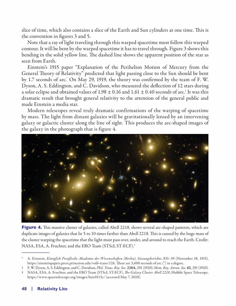
48 | Relativity Lite
slice of time, which also contains a slice of the Earth and Sun cylinders at one time. This is the convention in figures 3 and 5.
Note that a ray of light traveling through this warped spacetime must follow this warped contour. It will be bent by the warped spacetime it has to travel through. Figure 3 shows this bending in the solid yellow line. The dashed line shows the apparent position of the star as seen from Earth.
Einstein’s 1915 paper “Explanation of the Perihelion Motion of Mercury from the General Theory of Relativity” predicted that light passing close to the Sun should be bent by 1.7 seconds of arc.* On May 29, 1919, the theory was confirmed by the team of F. W. Dyson, A. S. Eddington, and C. Davidson, who measured the deflection of 12 stars during a solar eclipse and obtained values of 1.98 ± 0.16 and 1.61 ± 0.40 seconds of arc.† It was this dramatic result that brought general relativity to the attention of the general public and made Einstein a media star.
Modern telescopes reveal truly dramatic confirmations of the warping of spacetime by mass. The light from distant galaxies will be gravitationally lensed by an intervening galaxy or galactic cluster along the line of sight. This produces the arc- shaped images of the galaxy in the photograph that is figure 4.
Figure 4. This massive cluster of galaxies, called Abell 2218, shows several arc- shaped patterns, which are duplicate images of galaxies that lie 5 to 10 times farther than Abell 2218. This is caused by the huge mass of the cluster warping the spacetime that the light must pass over, under, and around to reach the Earth. Credit: NASA, ESA, A. Fruchter, and the ERO Team (STScI, ST- ECF).‡
* A. Einstein, Königlich Preußische Akademie der Wissenschaften (Berlin). Sitzungsberichte, 831– 39 (November 18, 1915), https:// einsteinpapers .press .princeton .edu/ vol6 -trans/ 126. There are 3,600 seconds of arc (") in a degree.
† F. W. Dyson, A. S. Eddington, and C. Davidson, Phil. Trans. Roy. Soc. 220A, 291 (1920); Mem. Roy. Astron. Soc. 62, 291 (1920).‡ NASA, ESA, A. Fruchter, and the ERO Team (STScI, ST- ECF), The Galaxy Cluster Abell 2218, Hubble Space Telescope,
https:// www .spacetelescope .org/ images/ heic0113c/ (accessed May 7, 2020).

Gravity Lite | 49
One other significant understanding comes from figure 3. The warping of spacetime around the Sun is the cause of the Earth moving around the Sun rather than flying off in the straight line its momentum would otherwise produce. This is much like the orbits a coin makes in the March of Dimes funnels one finds in public spaces. In this fashion, Einstein has replaced the idea of Newton’s gravitational force with a more fundamental explanation of events that predicts the motion of light as well as massive bodies.
One may find the limit of Einstein’s equations in the case of a small warping of spacetime, such as that caused by the Sun in the vicinity of the Earth, and the results agree perfectly with Newton’s “force.” But when gravitational effects become stronger, Newton’s descrip-tion becomes more and more inaccurate, whereas Einstein’s accurately predicts the state of affairs. Another key finding of Einstein’s 1915 paper was an explanation of the shift in the point of closest approach of the planet Mercury to the Sun, its perihelion. Since the 1850s astronomers had been trying to explain an anomalous extra 43 seconds of arc per century by which Mercury’s perihelion advances. In figure 5, the blue rosette shows this advance of the perihelion, much exaggerated.
Figure 5. NASA and MIT scientists analyzed subtle changes in Mercury’s motion to learn about the Sun and how its dynamics influence the planet’s orbit. The position of Mercury over time was determined from radio- tracking data obtained while NASA’s MESSENGER mission was active. Credit: NASA’s Goddard Space Flight Center.*
One may understand why Mercury’s perihelion advances by looking at a diagram of what is called the potential energy (PE) of its orbit. Potential energy is best understood by
* Elizabeth Zubritsky, “NASA Team Studies Middle- Aged Sun by Tracking Motion of Mercury,” National Aeronautics and Space Administration, last modified January 18, 2018, https:// www .nasa .gov/ feature/ goddard/ 2018/ nasa -team -studies -middle -aged -sun -by -tracking -motion -of -mercury.

50 | Relativity Lite
visualizing a marble rolling from one rim of a bowl down to the bottom, across that and up to the opposite rim, as in figure 6. This diagram is purely Newtonian, with no “bending of spacetime” to it.
The marble is momentarily motionless at the rim so it has no kinetic energy at that point. Newton’s “gravitational force” pulls it downward, and it gains speed. It moves its fastest across the bottom of the bowl— where it has zero potential to fall further and, thus, zero po-tential energy— so we say that it has pure kinetic energy during that passage. It loses speed as it climbs the far wall of the bowl, converting its kinetic energy into potential energy, so that when it reaches the opposite rim, it has no kinetic energy and maximal potential energy— perhaps understood as the potential to release energy back into kinetic energy as it rolls back down.
Figure 6. The transformation of potential energy into kinetic energy is demonstrated in Newtonian terms by a marble rolling in a bowl. In the initial position, the marble is temporarily still on the upper rim of the bowl on the right. Newton’s “gravitational force” pulls it downward, and it gains speed, rolling downward and transforming its potential to move into actual motion. This kinetic energy is greatest as it rolls across the bottom of the bowl, where its potential energy is zero. As it rolls up the left- hand wall, it loses kinetic energy and gains potential energy until it temporarily comes to rest on the opposite rim, where its potential energy is greatest.
This process is an expression of the law of conservation of energy: energy is neither cre-ated nor destroyed but simply converted from one form to another. Another example is the conversion of the stored chemical energy of gasoline into motion in a car upon combustion. Unfortunately, one cannot back up the car to get that energy back, nor will doing so retrieve the carbon the process releases into the atmosphere.

Gravity Lite | 51
Potential energy has more utility than just helping us understand how marbles roll in physical bowls. It is an alternative way to describe a Newtonian force that causes motion. The negative of the manner in which the potential energy changes with distance is the defi-nition of such a force. For instance, the potential energy curve for a pair of magnets whose north poles face each other looks like the left half of a U, with the horizontal position within the left half representing the closeness of the two magnets. The change in potential energy becomes more marked as one moves leftward on the left half of the U, so, by defini-tion, the magnetic force becomes more and more repulsive as you try to bring the two north poles together. It is repulsive because the change in PE is toward more positive values, and by definition, we take the negative of this positive change to get the direction of the force. Does the force encoded in that abstract description of the PE match your visceral experience of magnets?
The dotted red curve in figure 7 is a diagram of the Newtonian potential energy curve for the radius of Mercury’s orbit. One can imagine Mercury as a marble rolling back and forth in the depression. We have moved, here, from the case of a real marble rolling in a real bowl, under the influence of a real downward “Newtonian gravitational force” in figure 6, to an abstract marble rolling in an idea, called a potential energy curve in figure 7. In this abstract realm, it is the abstract principle that “systems seek to move to their lowest en-ergy state” that “pulls” the marble downward; not a real downward “gravitational force” (to the extent that we can say Newtonian approximations to Einsteinian spacetime constitute a “real” gravitational force).
But what is the nature of the rim on either side of that depression? Let me ask you a couple of questions. Mercury is moving so fast that it completes one orbit in 88 days. What is it that keeps Mercury from flying off into space? In Newtonian terms, it is the tug of gravity pulling it always inward: its tendency to fly off is continually checked by the force of gravity. The energy associated with this force depends on distance as 1/R. In Einsteinian terms, the only spacetime available for Mercury to travel through is a funnel so that it is constrained to move around and around the funnel. It would need more kinetic energy to rise higher up the funnel and, hence, farther from the Sun.
What is it that keeps Mercury from falling into the Sun? Its inertia; its tendency to keep moving in a straight line unless acted upon by a force. This is the “pseudo- force” that “slams” you into the door of a car turning a corner too sharply. We call this a pseudo- force because it is really the car’s door slamming into you as it turns while you try to continue moving in a straight line. In Newtonian terms, the outward pseudo- force of inertia must be perfectly balanced by the inward gravitational force for a planet to travel in a circular orbit. If you tie a rope to a brick and swing it around your head, you must exert an inward tug on a rope to counter the outward pseudo- force of the in-ertia of the brick— its desire to keep moving in a straight line toward your neighbor’s window.

52 | Relativity Lite
Figure 7. A diagram of the potential energy curve for the radius of Mercury’s orbit. The dotted curve is the Newtonian model, with the constraining peak near the origin arising from the square of Mercury’s angular momentum, ℓ. It also depends on the inverse square of the planet’s orbital radius, R, so the term gets bigger the smaller R becomes. To see this, divide 1 by 0.1 on a calculator to get 10. Squaring this gives 100. If you divide 1 by the even smaller value 0.01, you get an even bigger result, 100, and squaring this gives 10,000. One may continue on in this fashion. The solid blue curve is the general relativistic result, which has a new and negative term that likewise depends on the square of Mercury’s angular momentum. But this term depends on the inverse cube of the planet’s orbital radius, R. If you cube your division of 1 by 0.1 you get 1,000, and if you cube your division of 1 by the smaller value 0.01, you get 1,000,000. Since these terms have a larger size and are negative, they will at some small radius exactly cancel the Newtonian angular momentum term and for still smaller radii take this effect negative. This term dominates at small distances, bending the angular momentum barrier over into negative energies and thereby moving the barrier inward. Thus, under general relativity, Mercury spends more time at smaller radii, where it moves faster and therefore slides out of purely elliptical motion.
Consider the ice skater twirling with her arms outstretched. She will feel an outward force on her arms that her sinews must counteract. What happens when she pulls her arms in toward her body? Indeed, her spin will increase. But why is that? Just as with linear momentum, m v, which we explored in chapter 2, there is a quantity called angular momen-tum that is a conserved quantity. It is conventionally labeled with a script ℓ and defined as, ℓ = mvR, where R is the size of the object’s orbit. As the ice skater pulls her arms in toward her body, R becomes smaller, and in order to conserve angular momentum, v has to become larger to compensate (since m does not change). Thus, her spin will increase.

Gravity Lite | 53
We see then that the inertia that resists the pull of sinews or the pull of a rope or the tug of gravity on a planet is closely related to angular momentum. As the skater’s arms get closer to her body, conservation of angular momentum speeds her up. As Mercury, in its ellipti-cal orbit, gets closer to the Sun, it speeds up, and thus more effectively resists the inward pull of the stronger gravity in that region. We see that what keeps Mercury from crashing into the Sun at its closest approach is its angular momentum. That angular momentum is the left- hand “barrier” of the dotted red curve of the potential energy diagram in figure 7. This angular momentum barrier depends on distance as 1/R2 so that it will not have much effect at large distances, where the 1/R potential energy associated with the gravitational force dominates, but it will become larger than the gravitational potential energy at small distances. To see this, divide 1 by 10 on a calculator to get 0.1. Squaring this gives 0.01, a smaller value. If you divide 1 by the larger value 100, you get a smaller result, 0.01, and squaring this gives 0.0001, a much less influential amount.
What we have done in creating figure 7 is to fold into Mercury’s radial motion its motion around the Sun, manifesting the left- hand wall of the potential energy diagram that con-strains its motion toward the Sun, keeping it from getting too close. A “marble” rolling in this potential energy diagram will therefore oscillate back and forth between the inner and outer regions, modeling the radial motion of Mercury in its orbit.
The solid blue curve in figure 7 is the general relativistic result, which has a new term that depends in the same way on Mercury’s angular momentum as the Newtonian term. (This is one of those times when inserting lowest- order relativistic effects into a Newtonian framework pays off.) But it has a negative sign and depends on distance as 1/R3 so, at very small distances, it will dominate.
To see this, divide 1 by 0.1 on a calculator to get 10. Squaring this gives 100, the Newto-nian term. Cubing your division of 1 by 0.1 gives you 1,000 as the much larger Einsteinian term. If you divide 1 by the smaller value 0.01, you get a bigger result, 100, and squaring this gives 10,000. Cubing your division of 1 by 0.01 gives you 1,000,000 as the much larger Einsteinian term. One may continue on in this fashion. The Einsteinian term will dominate when R gets small enough and, since it is negative in sign, bend the angular momentum barrier over into negative energies and incidentally moving the barrier inward.
Even for modest distance, one sees that the inward motion of a marble rolling in the Ein-steinian potential energy curve is still constrained on the left, but not so strongly. The marble (Mercury) can come closer to the Sun than in the Newtonian case. It will spend more time in a region of stronger gravitational effects and will consequently have its orbit perturbed. The effect is not to make the orbit smaller or larger but to make it impossible for the orbit to close on itself. Mercury comes out of the point of closest approach shifted a bit to the side due to its penetration deeper into the Sun’s warping of spacetime. This precession of Mercury’s perihe-lion, which Einstein calculated in his 1915 paper to be 43 arc- seconds/century, matched the formerly unaccounted for 45 ± 5 arc- seconds/century of his day (and the more accurate 1947 value of 43.11 ± 0.45 arc- seconds/century*), which was strong evidence in favor of his theory.
* G. M. Clemence, Rev. Mod. Phys. 19, 361 (1947).

54 | Relativity Lite
BLACK HOLESStars maintain their size by balancing the inward gravitational force with the outward heat pres-sure supplied by nuclear fusion. In the core of the star (which is under high pressure due to the outer mass of the star pressing inward), pairs of hydrogen nuclei called protons are squeezed together to form deuterons, a pair of which are then transformed into one helium nucleus, a sort of process that gives off energy. This fusion will continue for 10 billion years in a star the size of our Sun until the hydrogen in the high- pressure core is used up. For another 150 million years,* helium is fused into carbon, but there is never enough heat to fuse carbon into the heavier elements. Without these nuclear fires, the Sun will no longer have the heat pressures to maintain its present size (large enough to fit a 1.3 million Earths inside), and it will ultimately shrink to about the size of the Earth. Such a star, called a white dwarf, maintains the new size only by the quantum- mechanical pressure of electrons that do not like to occupy the same quantum state, in part their position in space. We call this quantum effect a degeneracy force.†
For a star four times more massive than our Sun, there is sufficient pressure in the core to fuse carbon into oxygen, neon, and so on until iron is produced. The star then resembles an onion with hydrogen as the outer layer and iron at the core. Once iron is produced, it is no longer possible to fuse nuclei together to form heavier elements and give off energy. So the element production stops and the star begins to shrink. For these more massive stars, the quantum mechanical electron pressure (degeneracy force) is not enough to keep the star from collapsing past the white dwarf stage. The electrons will be jammed into the protons, converting them to neutrons (and neutrinos, such as those recorded in Supernova 1987a‡), and the star collapses inward until it is about 40 km across. At this point, the neutrons stop the collapse because they, too, do not like to occupy the same region of space. This star is called a neutron star, and it is so dense that “a thimbleful of neutron- star matter brought back to Earth would weight 100 million tons.”§
In the rapid gravitational collapse, there is a rebounding of the outer layers, a shock wave that has enough extra heat and pressure to transform some of the iron into heavier elements such as zinc. Thus, the heavy elements in your body were literally produced in a stellar explosion called a supernova. One or more supernovas some 6– 10 billion years ago scattered this material into the interstellar clouds of dust that eventually formed our Sun and planets. The interstellar shock wave of such explosions also helps trigger the coalescence of the solar systems out of this dust.
* Eric Chaisson and Steve McMillan, Astronomy Today, 2nd ed. (Prentice Hall, Upper Saddle River, NJ, 1996), p. 428.† For moderate- mass stars like our Sun, fusion of helium into carbon begins after the core collapses into this degenerate state.
Because the pressure in this nearly degenerate gas increases only slightly with temperature (Donald D. Clayton, Principles of Stellar Evolution and Nucleosynthesis [McGraw- Hill, New York, 1968], p. 103) the core does not reexpand for hours. But the fusion rate goes up with temperature to the 40th power (R. Robert Robbins, William H. Jeffreys, and Stephen J. Shawls, Discovering Astronomy [Wiley, New York, 1995], p. 388), so the core is a runaway fusion bomb for a few hours, called a helium flash. Finally, the carbon left in the core from helium burning shrinks until electron degeneracy sets in again and, for a moderate- mass star, never gets hot enough to fuse into heavier elements.
‡ K. Hirata et al., Phys. Rev. Lett. 58, 1490 (1987).§ That is, a density of 1014 g/cm3. William J. Kaufmann III, Discovering the Universe (W. H. Freeman, New York, 1989),
p. 289.
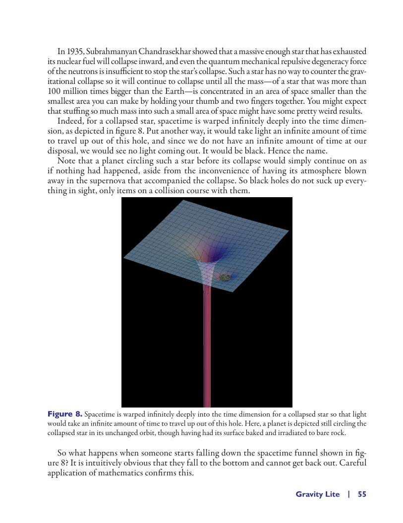
Gravity Lite | 55
In 1935, Subrahmanyan Chandrasekhar showed that a massive enough star that has exhausted its nuclear fuel will collapse inward, and even the quantum mechanical repulsive degeneracy force of the neutrons is insufficient to stop the star’s collapse. Such a star has no way to counter the grav-itational collapse so it will continue to collapse until all the mass— of a star that was more than 100 million times bigger than the Earth— is concentrated in an area of space smaller than the smallest area you can make by holding your thumb and two fingers together. You might expect that stuffing so much mass into such a small area of space might have some pretty weird results.
Indeed, for a collapsed star, spacetime is warped infinitely deeply into the time dimen-sion, as depicted in figure 8. Put another way, it would take light an infinite amount of time to travel up out of this hole, and since we do not have an infinite amount of time at our disposal, we would see no light coming out. It would be black. Hence the name.
Note that a planet circling such a star before its collapse would simply continue on as if nothing had happened, aside from the inconvenience of having its atmosphere blown away in the supernova that accompanied the collapse. So black holes do not suck up every-thing in sight, only items on a collision course with them.
Figure 8. Spacetime is warped infinitely deeply into the time dimension for a collapsed star so that light would take an infinite amount of time to travel up out of this hole. Here, a planet is depicted still circling the collapsed star in its unchanged orbit, though having had its surface baked and irradiated to bare rock.
So what happens when someone starts falling down the spacetime funnel shown in fig-ure 8? It is intuitively obvious that they fall to the bottom and cannot get back out. Careful application of mathematics confirms this.

56 | Relativity Lite
Isaac Newton showed in 1687 that the gravitational acceleration would be the same if all of a planet’s mass were concentrated at its center. Einstein said that acceleration due to thrusters and acceleration due to gravitation must be indistinguishable. So someone in a spaceship in orbit around a point- planet or collapsed star (figure 9) encounters the same bending of light as in figure 1a.
Figure 9. Gravitational acceleration would be the same if all of a planet’s mass were concentrated at its center, so the bending of light it causes would be the same.
We wish to know how the bending of light, and the consequent time dilation, depends on closeness to a star whose mass is all contained within a point. Since gravitational acceler-ation increases as one gets closer, the bending, too, will increase, with a picture something like figure 10.
∞∞∞∞∞ ←←←←←
r
s
cτct
r → r
Figure 10. Consider a sequence of versions of figure 1c, in which the acceleration is small at the top of the present figure (where r → ∞) and increasingly larger as one approaches the Schwarzschild radius rs, the distance from the singularity at which clocks appear to stop according to an outside observer. The length of the arc of the bent light gets longer and longer, for this sequence of versions of figure 1c, the closer one approaches the bottom of the figure, near the Schwarzschild radius rs.
There is no bending when one is far from the star (r → ∞ at the top of figure 10), and there is an infinite bending at the bottom as one approaches some, as yet undetermined, distance from the point in space where all the mass is concentrated. To get an intuitive sense that this distance is not zero requires some thought.

Gravity Lite | 57
What happens if I were to throw a pen straight up? (It goes up, stops, and then falls back down.) Suppose I wanted it to go higher. What would I do? (Throw it faster.) Suppose I wanted it to travel to an infinite height before it stops and falls down again. How fast would I need to throw it?
Pretend we are on an airless planet. The easy way to find this is to use energy conservation.Actually, let us run the movie backward. Suppose we have a pen sitting at infinity and
let it fall toward the Earth. How fast will it be moving just as it hits the surface? Let me just quote the result: the speed with which a pen falling from infinity would hit the Earth is
vGMRE
E
= =× × × ×
×
−2 2 6 67 10 5 106 378
11 24..m /s /kg .95 kg3 2
110
1 24 10 11 2
6
8 2
m
m2
v
s km s
E
= × =. / . /
*
* The derivation is not conceptually difficult, but it is long so I put it in this footnote for the curious. Feel free to ignore it.We introduced a formal definition of the potential energy of the gravitational field when we talked about a marble
rolling in a bowl (figure 6). You can see that that marble gains kinetic energy ( E mvK =12
2 from chapter 2) as it moves toward the bottom of the bowl and then loses it again as it climbs the far wall.
Likewise, if we look at comets in highly elliptical orbits about the Sun, they move very fast near the Sun and slow down as they move away. They give up the potential energy that they have far from the Sun, and it is converted into kinetic energy (higher speeds) near perihelion, and that kinetic energy is converted back to potential energy as they return to the outer edges of the Solar System. The potential energy of the Earth’s gravitational field at the surface is given by
EGMm
rP = − .Why the minus sign? Well, it is convenient to define the total energy,
E E mvGMm
rK P+ = −12
2 ,as being zero at infinity (where the pen is at rest for a moment),
E mGMm
i = −∞
= − =12
0 0 0 02 .Using energy conservation in this way we find that the final energy of the pen after falling from infinity will also sum
to zero:E mv
GMmRf E
E
= − =12
02 .
Adding the same thing to both sides of an equality will not change that equality, so12
02mvGMm
RGMm
RGMm
REE E E
− + = + ,
or12
2mvGMm
REE
= .Multiplying or dividing both sides of an equality by the same thing will not change that equality, so
2 12
22
mmv
mGMm
REE
= ,or
vGMRE
E
2 2= .
Taking the square root of both sides of an equality will not change that equality, so
vGMRE
E
= =× × × ×
×
−2 2 6 67 10 5 106 378
11 24..m /s /kg .95 kg3 2
1106 m.

58 | Relativity Lite
We can run this film forward and declare that 11.2 km/s is also the speed with which we would have to throw the pen to have it escape to infinity— its escape velocity.
Now suppose all the Earth’s mass were contracted to 1/100th its size, 64,000 m. What difference would this make in these calculations? The required velocity is 10 times bigger,
vGM
R
GMR
m sm
EE
64 00021
100
100100
2 100 10 11 200, , /= = = × = 1112 000, /m s
(We are allowed to multiply any expression by one without changing its nature, and in the square root, I multiplied by a convenient form, 1 = 100/100, which helped cancel the 1/100 in the denominator by which RE was multiplied to get this compacted mass. What remains is a factor of 100 in the numerator that we then pull out of the square root.)
Suppose all the Earth’s mass were contracted to 1/100th of 1/100th its original size, 640 m. What difference would this make in these calculations?
v640 m → 1,120,000 m/s
Suppose all the Earth’s mass were contracted to 1/100th of that size, 6.40 m.
v6.4 m → 11,200,000 m/s
Suppose all the Earth’s mass were contracted to 1/100th of that size, 64 mm.
v64 mm → 112,000,000 m/s
Suppose all the Earth’s mass were contracted to 1/100th of that size, 0.64 mm.
v0.64 mm → 1,120,000,000 m/s
Do you notice anything about the size of this velocity? What is the speed of light? We’ve just exceeded it!
We had better back up and find the smallest possible size into which the Earth could be crammed so that its escape velocity would be precisely c. It turns out to be about halfway between the last two examples, 8.89 mm.
The corresponding distance at which a photon could just escape a pinpoint containing all the Sun’s mass is the ratio of masses larger:
r mm mm kmS = = × =8 89 8 89 333 333 2 96. . , .MM
S
E
This is called the Schwarzschild radius— r GMcs =
22 = 2.953 km— found by Karl
Schwarzschild in 1916,* a year after Einstein published his general theory of relativity.† It
* K. Schwarzschild, Sitzber Deut. Akad. Wiss. Berlin, Kl. Math. Phys. Tech., 189– 96 (1916); 424– 34 (1916).† The final theory appears in his fourth paper of that year: A. Einstein, Preuss. Akad. Wiss. Berlin, Sitzber., 844– 47 (Decem-
ber 2, 1915).

Gravity Lite | 59
is fascinating to note that a dark- complected scientist and parson named John Mitchell predicted this result using Newtonian arguments in 1783.*
GRAVITATIONAL TIME DILATIONIn the section of chapter 2 entitled “The Low- Velocity Limit,” we read the Pythagorean theorem off of figure 1, c t c v t2 2 2 2 2 2= +τ , to give the exact expression for the time- dilation factor of special relativity:
γτ
= ≡
−
tvc
1
12
2
We wish to rewrite this in a pattern that will be useful for general relativity and for cosmology by squaring this and rearranging to
tvc
22
2
21
1=
−τ
For general relativity, the equivalent diagram, figure 1c, is much more difficult to solve for the length of t relative to τ. A great deal of mathematical work to find the length of this hyperbolic curve (see the appendix) gives
t
rGMc
2
2
21
1 1 2=− ×
τ
In the context of a black hole, t is the time measured by the astronaut near the Schwarzschild radius, and τ is that for an astronaut infinitely far away. The Earth- Sun distance is generally far enough away enough to give τ to good approximation.
In chapter 2, we saw that coordinate time t became infinitely dilated when v = c or, alter-natively expressed, when v2 = c2. If you compare the above two equations, looking for pat-terns as an artist might, you will notice that the position occupied by v2 in the first equation
is occupied by 1 2r
GM× in the second equation. Since there is order in mathematics, t must
become infinitely dilated when 1 2 2
rGM c× = , or alternatively expressed, when
1 22cGM r× = .
But this value of the distance is precisely the Schwarzschild radius r GMcs =
22 we just derived.
What this means is that the wristwatch on an astronaut approaching the Schwarzschild
* “The Country Parson Who Conceived of Black Holes,” American Museum of Natural History, https:// www .amnh .org/ learn -teach/ curriculum -collections/ cosmic -horizons/ case -study -john -michell -and -black -holes (accessed April 29, 2020).

60 | Relativity Lite
radius will slow down and stop as she or he reaches the Schwarzschild radius. You may see the details in this footnote,* if you wish.
On Earth we are not infinitely far away from a gravitating body, so we cannot actually measure proper time. But all we really need anyway is a relation that compares the time
* The easiest way to get meaning out of an equation is to look at its limiting values. For speeds v approaching 0, the first equation goes to
t 2 2 211 0
=−
=τ τ
That is, time is not stretched. The picture that corresponds to this equation is shown in the figure here. Since c t approxi-mately equals c τ in this picture and c is a constant, then t must approximately equal τ.
v t →→→→→ 0c
τ
c t
Likewise, if one goes an infinite distance from a black hole, 1/r goes to 0 in the second equation, and we have the same limiting equation above: time is not stretched. (The same limit applies if the mass M of the star is very small; there is not much spacetime warpage so we would expect the coordinate time to be about the same as proper time.)
This is most easily visualized by returning to the equivalent picture of a rocket being accelerated to the left. When the acceleration is near zero, the average velocity of a rocket starting from rest is also near zero. This is shown in the second figure in this note. Far from the black hole, the gravitational bending of light is so slight that the hyperbolic path c t cannot be distinguished from the hypotenuse of the figure, which is nearly the same length as the vertical leg c τ:
c τc t
as r →→→→→ ∞∞∞∞∞v t →→→→→ 0
average
If we go to the other extreme, for speeds v approaching the speed of light, the first equation goes to
t 2 2 211 1
10
=−
= = ∞τ τ
and coordinate time t becomes infinitely stretched compared to proper time τ as in the following picture:
v t
c τc t
Likewise, in the case of a black hole, the second equation says that as r approaches the value rGMcs =
22 , the Schwarzschild
radius, the denominator again goes to 1 − 1 = 0 so that coordinate time at that radius, ts , goes to infinity. This is the place in figure 10 where the hyperbolic path length for accelerated light c t stretches infinitely far to the right, relative to the vertical path length given by proper- time c τ that is measured at r = ∞ at the top of figure 10. Note that in this limit also, the hyperbola is nearly superimposed over the hypotenuse of the triangle in the figure below.
c τ
v t average
c t
Infinite gravitational time dilation happens at a finite value of r rather than at r = 0 because the speed of light is finite in the second equation, just as infinite time dilation happens at a finite value of v rather than at v = ∞ because the speed of light is finite in the first equation.

Gravity Lite | 61
dilation felt by two observers. Clearly an astronaut halfway down figure 10 (let us call him astronaut 1) will see a wristwatch worn by an astronaut near the bottom (let us call her astronaut 2) moving at a slower rate than his own. The slower frequency will cause light coming from the whites of her eyes to look reddish to him. We say that the light is gravi-tationally red- shifted. On the other hand, she will see the watch worn by astronaut 1, who is further away from the star, running faster than her own. Light from the whites of this astronaut’s eyes will look bluish to her. It has been gravitationally blue- shifted.
This means that if you wear a wristwatch and an ankle watch, the latter will literally run more slowly than the former. Since your ankle is only 1 m closer to the center of the Earth (6,378,000 m away) than is your wrist, and the mass of the Earth is relatively small, the difference is only 1 part in 5,000,000,000,000,000.* That is, you will age faster by one microsecond for every story (3 m) higher you live above the surface of the Earth.
The closer astronaut 2 gets to the black hole, the slower her watch will appear to run to astronaut 1. In fact, it would take an infinite amount of 1’s time for a second to pass on 2’s watch as she just approaches rs. Also, the closer she gets, the redder the light from the whites of her eyes will appear, passing in turn through red, infrared, microwave, and radio wavelengths until the wavelength would be so long as to be undetectable. Thus, we find that light cannot get out of the region inside rs, and that is why we call an object with such a sin-gularity in free space a black hole. Likewise, as astronaut 2 gets closer to the Schwarzschild radius, she sees the clocks on the spaceship far from the black hole carrying astronaut 1 spin faster. In fact, while 2 is having lunch, she would see that billions of years pass in the outside universe. The whites of astronaut 1’s eyes will become bluish, then give off ultra-violet radiation, then X- rays, and then gamma rays. Fortunately, her cone of observation simultaneously closes up so that the amount of this harsh radiation reaching astronaut 2 is diminished enough for her to survive it.
The biggest problem for astronaut 2 to worry about after lunch is that she will crash into, and become part of, the singularity at r = 0, the place where all the star’s mass is concen-trated. Einstein’s classical theory of gravity says that as she approached the singularity, it would have such a strong tidal effect that our poor astronaut would be stretched out to an infinite extent. However, quantum mechanics tells us that spacetime loses its smoothness as one experiences distances as small relative to the size of a proton as the proton is to us. Moving through distances this near the origin requires quantum jumps from one piece of a sponge- like space to another, as in figure 11c, a state of affairs not contained in Einstein’s classical theory of gravity.
* We can use the second equation twice to find the algebraic expression that represents this concept. If we say that observer 1 is at distance a r1 from the star and observer 2 is at distance r2 from the star. Then the coordinate times are related by
tGM r c
GM r ct1
12
22 2
1 2
1 2=
−
−
/
/. Because the Earth’s mass is small, this is approximately equal to t GM
r cr r
rt t1
22
1 2
12
1621 2 1 2 18 10� �
�
��
�
�� � ��� ��
��
�( ) . .
The red- shifting of light can be detected in light emitted from the surface of our Sun and seen on the Earth. If we had sensitive enough instruments to measure it, light coming from the surface of the Moon would be blue- shifted when seen on the Earth’s surface.
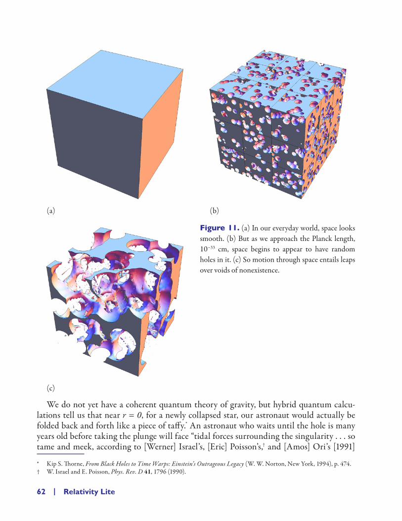
62 | Relativity Lite
(a) (b)
(c)
Figure 11. (a) In our everyday world, space looks smooth. (b) But as we approach the Planck length, 10−33 cm, space begins to appear to have random holes in it. (c) So motion through space entails leaps over voids of nonexistence.
We do not yet have a coherent quantum theory of gravity, but hybrid quantum calcu-lations tell us that near r = 0, for a newly collapsed star, our astronaut would actually be folded back and forth like a piece of taffy.* An astronaut who waits until the hole is many years old before taking the plunge will face “tidal forces surrounding the singularity . . . so tame and meek, according to [Werner] Israel’s, [Eric] Poisson’s,† and [Amos] Ori’s [1991]
* Kip S. Thorne, From Black Holes to Time Warps: Einstein’s Outrageous Legacy (W. W. Norton, New York, 1994), p. 474.† W. Israel and E. Poisson, Phys. Rev. D 41, 1796 (1990).

Gravity Lite | 63
calculations,* that the astronaut will hardly feel them at all. [Sh]e will survive, almost unscathed, right up to the edge of the probabilistic quantum gravity singularity. Only at the singularity’s edge, just as [s]he comes face- to- face with the laws of quantum grav-ity, will the astronaut be killed— and we cannot even be absolutely sure [s]he gets killed then, since we do not really understand at all well the laws of quantum gravity and their consequences.”†
There may even be a way to avoid a singularity completely. If the collapsing star were spinning, it would collapse onto a ring of no thickness (whose radius increases with the ratio of the rotational velocity to the mass of the black hole‡) rather than a point of no thickness.§ In fact, it’s very unlikely that a star would form with zero spin, or lose its spin as it collapses, so these Kerr black holes,¶ with their ring singularity, would be the norm. Our astronaut could conceivably pass through the center of the ring and miss the singularity. But then what?
Einstein’s equations allow a solution in which our astronaut would pass through the ring into a region called a white hole because time is reversed there so everything near the ring singularity travels out of a different one- way membrane into a flat region of our universe other than the one it started in or into another universe. I emphasized the word “allow” because one would actually have to “start” with the two flat regions of spacetime connected by a singularity so that the collapse of a star is unlikely to lead to such a wormhole.** No white hole has ever been seen.
Supposing such a wormhole is found, and our astronaut falls in, appearing redder and redder and seeming to take forever to do so to the outside world. She looks out and sees the outside universe appearing bluer and bluer and watches their clocks speed up. She sees an inconceivable number of years pass outside while it takes a few minutes of her time for her to pass through the wormhole into some other part of the same universe she left, in the
* A. Ori, Phys. Rev. Lett. 67, 789 (1991).† Kip S. Thorne, From Black Holes to Time Warps: Einstein’s Outrageous Legacy (W. W. Norton, New York, 1994), p. 479.‡ Robert M. Wald, General Relativity (University of Chicago Press, Chicago, 1984), p. 314– 15, gives the ring singularity at
rMc
=GJ
3 , where J is the total angular momentum of the collapsed star and its gravitational field (Steven Weinberg, Gravita-tion and Cosmology: Principles and Applications of the General Theory of Relativity [Wiley, New York, 1972], p. 240) and G is the gravitational constant.
§ For a spinning Kerr black hole, the surface of infinite time dilation and the one- way membrane are two different ellipsoidal surfaces,
whereas for a nonspinning black hole, these are combined into the spherical shell at the Schwarzschild radius. We will see infinite time dilation for an astronaut passing through the outermost ellipsoid of revolution, r+, but she could reemerge from this surface. The inner ellipsoid of revolution, r−, is the one- way surface of the Kerr black hole. Once she passes through r−, our astronaut is lost to us. But interestingly, maybe not lost to herself. See Ronald Adler, Maurice Bazin, and Menachem Schriffer, Introduction to General Relativity (McGraw- Hill, New York, 1975), p. 265.
¶ Roy P. Kerr, Phys. Rev. Lett. 11, 237– 38 (1963).** Robert M. Wald, General Relativity (University of Chicago Press, Chicago, 1984), p. 155.

64 | Relativity Lite
distant future, or perhaps into another universe. Figure 12 shows a wormhole connecting two regions of the same universe. With only two spatial dimensions shown, one is free to imagine the space portion bent around a curve in the time dimension and back the way it came. Thus, a trip that would take the spaceship eons by traveling leftward through space on the lower two- dimensional sheet— from a star near the wormhole, up around the curve, and back rightward— toward another star near the other end of the wormhole on the upper two- dimensional sheet could, in principle, be accomplished in much less time by traveling through the wormhole to the other two- dimensional spatial sheet, with the two openings of the wormhole separated by a time interval. The wormhole thus connects two very distant spatial places.
Figure 12. A wormhole connecting two distant regions of the same universe, with only two spatial dimensions shown.
Unfortunately, this would appear to be a one- way trip. Going back through would put her further into the future. So even if we had some brave volunteers to test these hypotheses, we would never know the answer.
GRAVITATIONAL WAVESIn 1916, Einstein predicted that the motion of massive objects would cause spacetime rip-ples, or gravitational waves. Figure 13 shows a pair of black holes orbiting each other, and their stirring of spacetime locally sends out an expanding ripple of gravitational waves.

Gravity Lite | 65
Figure 13. A pair of black holes orbiting each other would stir the spacetime they reside in, sending out an expanding ripple of gravitational waves that move at light speed. Only two spatial dimensions are shown, with the third being the time dimension.* Again, we have taken the additional liberty of showing just one slice of time. Had we let time flow upward as the third dimension here, the two holes would form a lovely collapsing spiral climbing upward, but the ripples would have been less easy to visualize.
The first clue that gravitational waves might be real was Russell Hulse and Joseph Taylor Jr.’s 1975 discovery of a pulsar orbiting a neutron star that was slowing down, apparently due to the emission of gravitational radiation waves,† work that later earned them the 1993 Nobel Prize. As the pulsar and neutron star lose energy via gravitational waves, they spiral inward over billions of years and will eventually crash into each other.
Explicit confirmation of the existence of gravitational waves from such a source came on September 14, 2015, thanks to the twin Laser Interferometer Gravitational- Wave Ob-servatory (LIGO) detectors located in Livingston, Louisiana, and Hanford, Washington, which each detected a passing gravitational wave. Figure 14 shows the characteristic sound of spacetime ringing as two black holes collide. In this final fraction of a second, the two black holes collide at nearly half the speed of light to form a single black hole and convert some of the mass of the black holes into wave energy. Only this peak energy is strong enough for LIGO to detect.
The signals came from two merging black holes lying 1.3 billion light- years away, one about 29 solar masses (29 times the mass of our Sun) and the other about 36 solar masses. The final, merged black hole was 62 times heavier than the Sun, and the remaining 3 solar masses were emitted as the energy of the massive gravitational wave crest that was detected.
* Modified from a Mathematica notebook by Jeff Bryant at https:// community .wolfram .com/ groups/ -/ m/ t/ 790989. He notes, “The function being plotted is not derived from any general relativity equations. It’s a very similar surface to the one used on the Wikipedia page for eLISA, and in fact was designed to try to emulate this.”
† R. A. Hulse and J. H. Taylor, Ap. J. 195, L51 (1975).

66 | Relativity Lite
On December 26, 2015, a second merger was detected from a pair of black holes 1.4 billion light- years away and which had about 14.2 and 7.5 times the mass of the Sun.
The 2017 Nobel Prize in Physics was awarded to three key figures in the development and success of LIGO: Barry Barish, Kip Thorne, and Rainer Weiss.
Figure 14. The signals of gravitational waves detected by the twin LIGO observatories at Livingston, Louisiana, and Hanford, Washington, from the merger of two black holes. The top signal at Hanford arrived 1/7000th of a second after the signal first reached Livingston, the middle plot, which shows that it traveled at the speed of light. The bottom plot compares data from both detectors, with the Hanford data shifted by that time interval and inverted to account for the different orientation of the detectors at the two sites.
The signals, including the instruments’ ever- present noise, were compared against numerous simulated signals, based on the equations of general relativity, varying by mass and distance. The best fit was for a merger of two black holes— one about 29 times the mass of the Sun and the other about 36 solar masses— lying 1.3 billion light- years away. This comparison is shown in white. Time is plotted on the x- axis and strain on the y- axis. Strain represents the fractional amount by which distances are distorted— less than the width of a proton. Image credit: Caltech / MIT / LIGO Lab.*
* “Gravitational Waves, as Einstein Predicted,” LIGO Laboratory, https:// www .ligo .caltech .edu/ image/ ligo20160211a (ac-cessed May 7, 2020).
Cosmology | 67
CHAPTER 5
CosmologyTHE BIG BANGOne of the more interesting applications of the general theory of relativity is in cosmology. In 1927, Georges Lemaître published a paper attempting to reconcile the massless cosmo-logical solution of general relativity by Willem de Sitter, which explained “the observed receding velocities of extra- galactic nebulæ,” and Einstein’s own solution containing mass but including a cosmological constant to make for a static universe. Lemaître’s solution did reconcile them and provided a value for the relation between the recessional velocities of the galaxies and their distances, 625 km per second for every 1 million parsecs the galaxies are away from us.* That is, nearby galaxies are sluggishly moving away from us, while the farthest galaxies are sprinting.
Two years later, Edwin Hubble (after whom the space telescope is named) used his own improved observations to derive a more accurate constant. Hubble’s work became widely known, while Lemaître’s prior explication of what became known as the Hubble law did not, in part because Lemaître left his value out of the 1931 English translation, since he felt that better values had subsequently been offered.† It was only in 2018 that the Interna-tional Astronomical Union (IAU) recommended that the law henceforth be known as the Hubble– Lemaître law.
This law suggests that we may be in the middle of some cosmic explosion of galaxies. In 1936, Robertson and Walker found a solution to Einstein’s equations in which the uni-verse could have expanded outward from an infinitely dense state.‡ In 1948, Ralph Alpher and Robert Herman showed that as this expanding universe cooled from its inconceivably high initial temperature to a mere billion degrees in the first 200 seconds or so, about 1/4 of the hydrogen nuclei would have been transformed into helium nuclei. This is exactly
* G. Lemaître, Annales de la Société Scientifique de Bruxelles A47, 49– 59 (1927).† The relevant passage in the original is “Utilisant les 42 nébuleuses figurant dans les listes de Hubble et de Strômberg (1),
et tenant compte de la vitesse propre du soleil (300 Km. dans la direction α = 315°, δ = 62°), on trouve une distance 0,95 millions de parsecs et une vitesse radiale de 600 Km./sec, soit 625 Km./sec à 10° parsecs (2).” Abbé G. Lemaître, MNRAS 91, 483– 90 (1931).
‡ H. P. Robertson and A. G. Walker, Proc. London Math. Soc. 42, 90 (1936).

68 | Relativity Lite
the proportion of helium to hydrogen that is observed in the universe. They also estimated that this cooling would have continued for the subsequent 15– 20 billion years until today, when one should see the ghost of this explosion as microwave radiation with a temperature of about 5 degrees above absolute zero, or 5 Kelvins (K; room temperature is 300 K).* In 1965, Arno Penzias and Robert Wilson observed this background microwave radiation at a temperature of 3 K,† so the Big Bang appears to be confirmed.
You actually know enough now to see how a Big Bang would work. Throughout this book, we have been using a pattern in which we relate proper time to coordinate time and coordinate distance. In chapter 1’s discussion of special relativity, we saw that the Pythago-rean theorem applied to the light path in a ship moving at speed v relative to the Earth gave the full spacetime relation for proper time,‡
τ 2 22
21= −t
cr (1)
For an accelerating rocket ship, or the equivalent observer in a gravitational field, the equivalent relation is
τ 22
2
22
21 2 1
1 2= −
−−
+GMrc
tc GM
rc
r angular terms (2)
where a full accounting would include angular spatial terms§ as well as the radial one we concentrated on in chapter 4, but those play no part in the discussion that follows.
Comparing this with time dilation in special relativity, you may see a symbolic pattern emerging in the shape of the equations, even had you not gone through the details of the idea in pictures. For the Robertson- Walker relation that describes the expansion of the uni-verse, we might expect to see some quantity that changes with coordinate space and time multiplying the t2 term minus another quantity multiplying the r2 term. It turns out that the correct relation is
τ 2 2 22 2
211
= −−
+t Rkr c
r( )
angular terms (3)
R is a quantity that changes with time (often expressed by the notation R(t)) and so shows us how the intergalactic distances involving r and angles change with time. This cos-mic scale factor is most easily thought of as the radius of a four- dimensional cosmic balloon, a hypersphere, that has as its outer surface our three- dimensional space. Now we do not have the ability to draw a four- dimensional balloon, but we can get an idea of how this would
* R. A. Alpher and R. C. Herman, Nature 162, 774 (1948); Phys. Rev. 75, 1089 (1949).† A. A. Penzias and R. W. Wilson, Astrophys. J. 142, 419 (1965).
‡ We can set v t = r in τ 2 22
2 2 22
21 1= − = −t
cv t t
cr .
§ See, for instance, Ronald Adler, Maurice Bazin, and Menachem Schriffer, Introduction to General Relativity (McGraw- Hill, New York, 1975), p. 225.
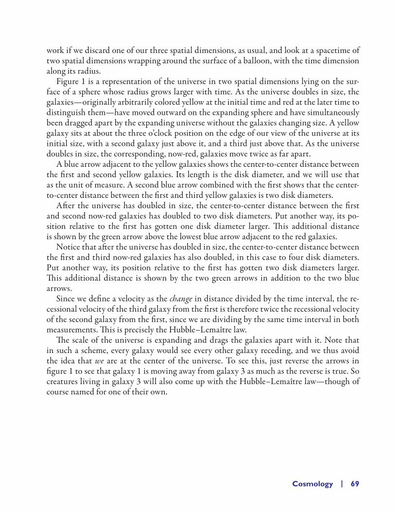
Cosmology | 69
work if we discard one of our three spatial dimensions, as usual, and look at a spacetime of two spatial dimensions wrapping around the surface of a balloon, with the time dimension along its radius.
Figure 1 is a representation of the universe in two spatial dimensions lying on the sur-face of a sphere whose radius grows larger with time. As the universe doubles in size, the galaxies— originally arbitrarily colored yellow at the initial time and red at the later time to distinguish them— have moved outward on the expanding sphere and have simultaneously been dragged apart by the expanding universe without the galaxies changing size. A yellow galaxy sits at about the three o’clock position on the edge of our view of the universe at its initial size, with a second galaxy just above it, and a third just above that. As the universe doubles in size, the corresponding, now- red, galaxies move twice as far apart.
A blue arrow adjacent to the yellow galaxies shows the center- to- center distance between the first and second yellow galaxies. Its length is the disk diameter, and we will use that as the unit of measure. A second blue arrow combined with the first shows that the center- to- center distance between the first and third yellow galaxies is two disk diameters.
After the universe has doubled in size, the center- to- center distance between the first and second now- red galaxies has doubled to two disk diameters. Put another way, its po-sition relative to the first has gotten one disk diameter larger. This additional distance is shown by the green arrow above the lowest blue arrow adjacent to the red galaxies.
Notice that after the universe has doubled in size, the center- to- center distance between the first and third now- red galaxies has also doubled, in this case to four disk diameters. Put another way, its position relative to the first has gotten two disk diameters larger. This additional distance is shown by the two green arrows in addition to the two blue arrows.
Since we define a velocity as the change in distance divided by the time interval, the re-cessional velocity of the third galaxy from the first is therefore twice the recessional velocity of the second galaxy from the first, since we are dividing by the same time interval in both measurements. This is precisely the Hubble– Lemaître law.
The scale of the universe is expanding and drags the galaxies apart with it. Note that in such a scheme, every galaxy would see every other galaxy receding, and we thus avoid the idea that we are at the center of the universe. To see this, just reverse the arrows in figure 1 to see that galaxy 1 is moving away from galaxy 3 as much as the reverse is true. So creatures living in galaxy 3 will also come up with the Hubble– Lemaître law— though of course named for one of their own.

Figure 1. A representation of the universe in two spatial dimensions as lying on the surface of a sphere whose radius grows larger with time. The yellow disks lying on the inner sphere represent galaxies whose diameters are extremely exaggerated in size relative to the circumference of the universe. As the universe doubles in size, the galaxies— now red to distinguish the two times— have moved outward on the outer surface and have been dragged apart by the expanding universe without the galaxies changing size. A yellow galaxy sits at about the three o’clock position on the edge of our view of the universe at its initial size, with a second galaxy just above it and a third just above that. As the universe doubles in size, the corresponding, now- red, galaxies move twice as far apart.
The blue arrows adjacent to the yellow galaxies may be used to count the center- to- center distance between the first, second, and third galaxies as the universe expands. The green arrows add to the blues ones and represent the change in distance, which we divide by the time interval to get the recessional velocities. The distance from the first to the third galaxy has grown by two green arrows, while the distance from the first to the second galaxy has grown by only one green arrow, so the recessional velocity of the third from the first is twice that of the second galaxy from the first. This is the meaning of the Hubble– Lemaître law.

Cosmology | 71
Figure 1 also shows that the sizes of the galaxies (disks) do not change as their distance apart grows, nor do our local rulers grow with time, nor our noses. This is true for two rea-sons. First of all, the expansion equations showing an expanding universe are based on the idea that the universe is homogeneous, which holds true only on a large scale. The universe is decidedly lumpy on the scale of galaxies, solar systems, rulers, and atoms. Second, even if we could prove that a lumpy cosmology would expand, the gravitational attraction of nearby stars would overwhelm any cosmic tendency for galaxies to expand. And our bodies are held together by electrical forces that are (locally) enormously stronger than gravitational ones. (Otherwise we would fall through the chairs we sit on.) However, in an accelerating expansion that we will discuss in a minute, both local gravity and even electrical attraction may eventually be overwhelmed.
Finally, the question always comes up, “What is the universe expanding into?” If we were living in the universe of figure 1 in the yellow- galaxy era, there would be no outer surface with red galaxies sitting on it. We could take a photograph inward from our surface into the past, but to photograph outward would be to photograph the future, and that is something no one I know is skilled at. From this perspective, one might say, “There is noth-ing there for the universe to expand into, and by ‘nothing’ I don’t mean emptiness of some sort but nonexistence. The universe must make the universe it is expanding into!”
Remember that figure 1 is a representation of the universe in two spatial dimensions lying on the surface of a sphere whose radius grows larger with time. Put another way, in this picture, time is synonymous with the radius of the sphere. As time gets big, the sphere’s radius gets big in exact proportion. So for a spherical universe, one might answer, “The universe is expanding into the future!”
If you are satisfied with the Hubble– Lemaître law as given above, you may skip the fol-lowing section that actually proves the Hubble– Lemaître law using some fairly complicated visual relationships.
THE HUBBLE– LEMAÎTRE LAWWe can show how the Hubble– Lemaître law works in more detail using figure 2, a cross sec-tion of the four- dimensional hypersphere of figure 1, but now with the added complication of a universe that is slowing its expansion velocity as time progresses. This slowing is what one would expect as the mass of all the rest of the universe tugs backward on the speed of every individual galaxy.

Figure 2. Consider the cross section of a spherical, expanding universe whose expansion rate S is slowing with time. R is the cosmic scale factor and, in the spherical case, is equal to the radius of the sphere. D is the arc of a circle, giving the distance between two galaxies exactly 60° around the curve from each other. V is the recessional speed of one galaxy, at the 2 o’clock position, from the one at the 4 o’clock position around the circumference of the circle— the change in D with time. The distance D at time 1, D(1), has been duplicated and shifted outward and placed next to D(2). The additional distance that must be added to D(1) to make the full distance D(2) is one time unit multiplying V(2), the recessional velocity at time 2. As the universal expansion slows, the recessional velocities also get smaller at times 3 and 4.
It may be easier to see distances and their changes over time by looking at equilateral triangles rather than arcs of circles. Thus, we also show C, the chord of the arc D, adjacent to a different 60° pie slice for visual clarity. The corresponding change in chord length from C(1) to C(2) with time is one time unit multiplying the velocity U(2). Since the chords are proportional to the arcs, U(2) is therefore proportional to the actual recessional velocity V(2).

Cosmology | 73
For a galaxy at the 12 o’clock position, exactly 60° around the curve from where we are at the 2 o’clock position in figure 2, the distance across the chord between the galaxies equals the radius of the universe, because they are two sides of an equilateral triangle. This is true for any time: C(t) = R(t). Then the velocity U, the change in C with time, is precisely the expansion speed of the universe (the change in R with time) in this 60° case, or U(t) = S(t). Let us define a Hubble constant (as it is called, though it changes with time) at the present time H(4) = H0 as the ratio of the present expansion speed divided by the present radius: H0 ≡ S(4)/R(4) = U(4)/C(4) for galaxies in this 60° case. The Hubble– Lemaître law is simply a rewriting of this relation, giving the recessional velocity as proportional to the distance, U(4) = H0 C(4), with H0 as the constant of proportionality.
The actual distances between, and velocities of, galaxies are along the circumference, not across the chord, but those are in proportion. We check this by using the arc lengths in figure 2, laid out in a different 60° pie slice for visual clarity, using a galaxy at the 4 o’clock position exactly 60° around the curve from where we are at the 2 o’clock position. It turns out that an arc of a circle has length R θ, where the angle θ is expressed in fractions of the circumference (2 π R) of a circle that has radius 1, and thus as fractions of 2 π. For our case, 60° is 1/6 of the circumference so θ = π/3 = 1.05 to three decimal places. (As you eyeball figure 2, you might agree that the arcs could be about 5% larger than the chords.) As noted in the previous paragraph, the length of the chord across this 60° arc is precisely R, because they are two sides of an equilateral triangle. The adjacent arc has length 1.05 R for our 60° case. So if we just multiply all chord lengths C and their corresponding velocities U by 105%, we get the actual galactic distances D and recessional velocities V. But since we are taking ratios, this factor of 1.05 cancels out for any time: V/D = (1.05 U)/(1.05 C) = 1.05/1.05 U/C = 1 U/C = S/R = H0, or V = H0 D.
The arcs have the advantage of being able to be divided into smaller pie wedges whose arc lengths are easily seen. Suppose we imagine a galaxy at the 3 o’clock position at time 4, only 30° around the curve from where we are at the 2 o’clock position. Its distance from us will be half of D(4). We can also split the corresponding recessional velocity V(4) up into two parts, half associated with the 4 o’clock galaxy’s motion away from the 3 o’clock galaxy, and half associated with the 3 o’clock galaxy’s motion away from us at the 2 o’clock position. Looking at each half, we see that (D(4)/2)/(V(4)/2) = D(4)/V(4) = H0 yet again, so the Hubble– Lemaître law holds for galaxies at any distance from us.
We are used to seeing the relationship between velocity and distance written as D = V T, so we see that the Hubble constant is the inverse of some time, H0 = 1/T. T turns out to be an estimate of the age of the universe, good to about 60% accuracy.

74 | Relativity Lite
BUT IS THE UNIVERSE A FOUR- DIMENSIONAL SPHERE?The constant k in equation (3) tells us about the shape of the universe. The balloon scenario is accurate only if k = +1. Since this universe has no edge, if you waited long enough, you would eventually see light from the back of your head that had traveled all the way around the four- dimensional hypersphere to your eyes.
If k = −1, then space is infinite and boundless, part of which is the saddle shape shown in figure 3.
(a) (b)
Figure 3. A saddle- shaped universe also expands as the parameter R increases.
For k = 0, equation (3) looks very much like equation (1), with only the addition of the scale factor R that allows the universe to grow with time. Thus, in this case, as for special relativity, space is flat. For this to be the case, the density of the universe must be at a critical
value given by the Hubble constant and Newton’s gravitational constant G as ρπcH
G=
38
02
.
For a spacetime like that given by the Robertson- Walker metric equation (3) (and more generally, Friedmann– Lemaître spacetimes), something called the Friedmann equation gives the expansion velocity of the universe. In the matter- dominated era, it can be shown that the square of the ratio of the expansion velocity of the universe S to the speed of light is
S2/c2 = Rmax/R − k. (4a)
When we look at the Hubble expansion in a k = 1 universe, we see that the expansion velocity S goes to zero at
R = Rmax, (5)

Cosmology | 75
since one then would have S2/c2 = 1 − 1 = 0. (Here Rmax is given* in terms of the current radius R0 and current density ρ0 of the universe as 8 π G/3 ρ0 R0
3/c2, in which we must have ρ0 > ρc for k to be 1.) But the mass is still exerting a force on the universe when it has stopped expanding, so we have a big crunch coming.
For those of you not familiar with looking for patterns in equations with your mind’s eye, let us cast equation (4a) into a form for more conventional vision. If we arbitrarily set Rmax = 4, then as R increases from 0 to 10, the ratio Rmax/R drops from a high value to 0.4 at R = 10. This is the second picture in equation (4b). Next we have k = 1 for all R from 0 to 10, the third picture in equation (4b). If we subtract off the third picture from the second picture, we get the first picture, S2/c2, with the dropping curve shifted downward by 1 unit at every point and becoming 0 at R = Rmax = 4:
(4b)
When we look at the Hubble expansion in a k = 0 universe, the only value of R that will make S2/c2 = 0 in equation (4a) is R = ∞, as one can see by trying a series of larger values of R for Rmax arbitrarily set to 4 units: 4/100 = 0.04, 4/1000 = 0.004, 4/10000 = 0.0004, and so forth.
This is also seen in the k = 0 universe pictured in equation (4c). We have extended R 10 times farther than in equation (4b), and even at R = 100, the curve seems already at 0. In this case, the third picture has k = 0 for all values of R, so the subtraction of 0 does nothing, and the first picture for S2/c2 just duplicates the second one, going to 0 as R → ∞:
(4c)
When we look at the Hubble expansion in a k = −1 universe, subtracting a negative is equivalent to adding a positive (−(−1) = +1) and there is no value of R that will make S2/c2 = 0, since we will always have the 1 left over, however small Rmax/R becomes. In equa-tion (4d), the first picture has the Rmax/R of the second picture shifted upward to approach 1. This universe will go on expanding forever.
* Tai L. Chow, Gravity, Black Holes, and the Very Early Universe an Introduction to General Relativity and Cosmology (Springer, New York, 2008), p. 142, eq. (8.42).

76 | Relativity Lite
(4d)
So now we must somehow choose which shape (k = 1, 0, or −1) fits our universe.
THE BANGOne naturally wonders why the universe is expanding at all. Indeed, we can run the movie backward in our imagination, seeing the galaxies coming closer together as we move back-ward in time, as in figure 4. Their initial, yellow, configuration becomes denser as time goes backward, with galaxies overlapping as the universe shrinks to a third of that size, shown in blue. As time runs down to zero, the spacetime containing the matter that makes up the galaxies turns into an infinitely dense dot that would also be extremely hot due to the friction of the jostled particles as they are forced into a smaller and smaller volume.
Figure 4. If we run time backward, the galaxies in their initial, yellow, configuration grow closer together, indeed overlapping as the universe shrinks to a third of that size, shown in blue. As time runs back to zero, the density of matter in galaxies becomes infinite and extremely hot.

Cosmology | 77
Such a visualization led to the idea of the Big Bang— that an initial singularity of in-finitely dense, hot matter somehow exploded outward and is continuing to fly outward to this day, cooling as it expands.
AN OPEN AND SHUT CASEWhat would cause the shape of the universe to curve in on itself, as in figure 1, or flop open, as in figure 3, or to take on perfect flatness? One may profitably ask a parallel question, “What causes an umbrella to close?” Well, you cause it to close by pulling down on the ring surrounding the handle, which in turn tugs inward on the spokes that attach to the cloth- covered ribs. There are a few umbrellas that I have had a pretty hard time closing because I could not exert sufficient force to counter the outward pressure of the spring.
Suppose you had a universe that had enough mass that the inward gravitational force (in Newtonian language) could slow the outward expansion, bring it to a halt, and then cause it to recollapse in a Big Crunch. This is the k = +1 case. Suppose you had a universe that had insufficient mass to counter the outward momentum of the explosion of galaxies that is the Big Bang. That universe would not curl in on itself into a sphere but stay open like a floppy umbrella. This is the k = −1 case. There would, then, be some critical density of
matter, ρπcH
G=
38
02
, just sufficient to halt the outward expansion at infinite time. This is the
k = 0 case.*We saw in the last section that running the closed, spherical- universe, k = +1 case back-
ward in time led to an infinitely dense pinpoint singularity from which the Big Bang ex-panded outward. What about the other two, the open- and critical- universe cases where our universe is presently a saddle shape of infinite extent or flat and infinite? As one looks at figure 5, one sees in either case a universe at present at the top becoming denser and denser as one proceeds downward, back in time.
No matter how far to the left the galaxies move, as we go backward in time to create increasing density, there will always be an infinite number of additional galaxies to the right moving into our frame of view. Thus, we can have an infinitely dense universe that is infinitely large just before the Big Bang occurred.
So in the k = 0 or k = −1 cases, the universe would not all be stuffed within a single point, as it would be if k = +1, but the entire infinite universe is nevertheless infinitely dense. In these cases, the Big Bang did not expand from a single point but from everywhere in the universe, and the scale of the universe, R, has been increasing ever since.
* Before rescaling r to give k unit magnitude, k is given by k
RG
c c02 2 0
83
= −( )πρ ρ where ρ
πcH
G=
38
02
is the critical density, ρ0 is
the present density of the universe, R0 is its present size, H0 is the Hubble constant, and G is the universal gravitational constant.

78 | Relativity Lite
pr esent time
7 bi l l ion year s ago
near the timeof the big bang
1 mil l ion l ight year s between galax ies
near infinite density of galax ies an infinite number of galax ies to the r ight
t
Figure 5. Even in the case of a universe that always was of infinite size, one can see an infinitely dense early universe by projecting present galactic density backward in time.
For the k = 0 or k = −1 cases, we can again ask, “What is the universe expanding into?” Well, for these cases time is not synonymous with the radius of a sphere. In figure 5, time points straight up and the galaxies are moving rightward. So the expansion is not into the future, nor does the universe create the universe it is expanding into. We can say, “The uni-verse was already infinite at the start so there is plenty of universe for the universe to expand into, is there not?” This is best explicated by part of a story of two travelers checking into a hotel, modeled on David Hilbert’s ideas of infinity:
“We’re completely full, sir. Not even a dog kennel to spare. In fact, the dog seems to have double- booked his kennel to a pack of huskies.”
Smith gestured at their huge pile of luggage. “Well, we’re not equipped for camping on the beach. We’ve got to stay somewhere!”
The receptionist nodded in sympathy. “Mmm, . . . I’ve got an idea, sir. But it will mean a bit of disruption . . . Let me check with the Manager.” She hurried off. About ten minutes later she returned, smiling broadly. “You’re in luck, Room 1 has just become vacant.”
“Brilliant.” A thought occurred to Smith. “Where are they going, then? You said the airport’s closed.”
“Into Room 2.”“But Room 2 is occupied.”“No, they’re moving into Room 3.”

Cosmology | 79
“And where are they going?”“Room 4, of course. We’ve relocated the people in Room 4 to Room 5. In fact, we’ve moved
everybody up one room number.”Smith felt his head spinning. “But . . . but what about whoever’s in the last room?”“Ah, I see you’re labouring under a misconception. This is a Hilbert Hotel. There is no last
room. We have infinitely many rooms— 1, 2, 3, and so on forever. Right now, of course, they’re all full because we have infinitely many guests. But infinity plus one is still infinity, so we can rearrange the guests to create an extra room for you.”*
Thus, the answer to our question is tied up with the question of just which universe we are living in and does not seem to be answerable apart from that.
COSMIC INFLATIONIn 1964, Peter W. Higgs proposed a mechanism to account for the existence of massive particles arising from the massless ones so far predicted by our theories.† One might roughly think of this Higgs field permeating all space acting as a drag on the motions of particles, making them more ponderous, as we are when we are walking in a swimming pool. Carl Hagen, Gerald Guralnik, and Tom Kibble also published a paper a month later on this top-ic.‡ Francois Englert and his colleague Robert Brout, who died in 2011, actually published their version two months before the publication of Higgs’s paper.§ But Higgs was the only one of the six who explicitly suggested that a particle would be associated with this field, whose spin would be zero (a class of particles known as bosons),¶ so his name was attached to that particle and via that to the field.
The Higgs boson was confirmed on July 4, 2012, at the CERN particle accelerator.** In 2013, Higgs and Englert were jointly awarded the Nobel Prize in Physics for their theories. (The rules of the Nobel stipulate that recipients be living persons, excluding Brout, and going to a maximum of three recipients, preventing the trio of Hagen, Guralnik, and Kib-ble from being added. In 2010, all six were awarded the J. J. Sakurai Prize for Theoretical Particle Physics.)
What would be the effect on the evolution of the Big Bang if there were a Higgs field permeating all space? In 1981, Alan Guth suggested that such a field would have a profound
* Ian Stewart, New Scientist 160, 58 (1998).† Peter W. Higgs, Phys. Lett. 12, 132 (1964); Phys. Rev. Lett. 13, 508 (1964).‡ G. S. Guralnik, C. R. Hagen, and T. W. B. Kibble, Phys. Rev. Lett. 13, 585 (1964).§ F. Englert and R. Brout, “Broken Symmetry and Mass of Gauge Vector—Mesons,” Phys. Rev. Lett. 13, 321 (1964).¶ See “Interview to Prof. Peter Higgs About the Latest Results on the Searches for the Higgs Boson at the LHC,” CERN,
July 4, 2012, http:// cds.cern.ch/ record/ 1459437.** “New Results Indicate That Particle Discovered at CERN Is a Higgs Boson,” CERN, March 14, 2013,
https://home.cern/news/press-release/cern/new-results-indicate-particle-discovered-cern-higgs-boson.

80 | Relativity Lite
effect on the early expansion of the universe:* the negative pressure of the Higgs field would produce a repulsive gravitational force that would overpower its own inward tugging on spacetime once the density of the universe became low enough. Within 10−35 seconds the universe would double 100 times to become 1030 times its original size!† Andreas Albrecht with Paul Steinhardt and Andrei Linde, proposed modifications that account better for the production of a hot fireball at the end of this inflationary expansion that would look very much like the standard Big Bang.‡
WHY WOULD THE HIGGS FIELD PRODUCE A NEGATIVE PRESSURE, AND WHY WOULD THIS OPPOSE GRAVITY?One of the fascinating facets of quantum mechanics is Heisenberg’s uncertainty principle, which says that one cannot know both a particle’s position and its momentum with absolute certainty. Imagine, for instance, shining light on a tiny particle so that one may see it in a microscope. One would like to use light with a short wavelength, since objects have to be bigger than, or roughly the same size as, the distance between light wave crests in order to be seen. But unfortunately, short wavelength light, such as ultraviolet (UV) radiation, has higher energy and momentum§ than long wavelength light, such as infrared (IR) light. So imaging the particle with UV would allow one to see where the particle is more easily, except that UV will also kick it away from the light source so that one has less of an idea of where it is after the attempt. On the other hand, imaging the tiny particle with IR would help keep the particle more in place while we image it, but IR waves are so long that we can-not use them to see the particle if that particle is small enough. This difficulty is a physical manifestation of the uncertainty principle.
Given that energy and time are related in relativity to momentum and position, one should not be surprised that an uncertainty principle involving time and energy also ap-pears in quantum mechanics. One of the most interesting manifestations of this is that one may violate our certainty that energy is conserved as long as one does so for a very short time. It turns out that what we think about as the emptiness of spacetime constantly has pairs of electrons and their antimatter partners, called positrons, springing into existence, existing for a very short time, and then annihilating each other, giving back the energy they “borrowed” from the universe in order to come into being. Virtual protons and antiprotons likewise spring into existence in empty space, in the room before us, and in between our
* Alan H. Guth, Phys. Rev. 23, 347 (1981).† Alan H. Guth, The Inflationary Universe: The Quest for a New Theory of Cosmic Origins (Addison Wesley, Reading, MA,
1997), p. 171– 77.‡ Andreas Albrecht and Paul J. Steinhardt, Phys. Rev. Lett. 48, 1220 (1982); Andrei D. Linde, Phys. Lett. B 175, 395 (1986).§ Yes, massless particles have momentum. In general, the ratio of momentum to energy is, from figure 3 of chapter 2,
pE
mvmc
vc
= =γγ2 2 . For light, v = c so
pE
cc c
= =2
1, or p = E/c.

Cosmology | 81
ears and live for a short enough time, within the uncertainty principle, that they do not ultimately violate energy conversation.
Dutch physicist Hendrik Casimir* predicted in 1948 that if one were to put two un-charged metal plates close enough together, the larger varieties of virtual particle pairs that can spring into being outside the plates, compared to those that can in between them, will tend to push the plates together. This prediction was confirmed in 1997 by S. K. Lam-oreaux.† The vacuum is, thus, not empty at all; it has energy.
SYMMETRY BREAKINGIn 1918, a German mathematician named Emmy Noether discovered and published what is the most profound theorem on symmetry to date. She gave us a relation between symmetries and conservation laws. A spinning ice skater who pulls her arms in speeds up. Why is this? She has angular momentum as she spins, which is a product of her mass, the speed of her spin, and the distance of her mass from the spin axis. As she pulls her arms in, the distance of part of her mass from the spin axis decreases, and the only thing one may balance this change with to keep her angular momentum constant is to speed her up.
But there is a deeper why to this. Noether showed that angular momentum conservation is a consequence of the symmetry (angular uniformity) of the space surrounding the skater. She showed that if you turn through an infinitesimal angle, the difference of kinetic and po-tential energies— which is called the Lagrangian— is unchanged. By adding up a bunch of zero changes for a bunch of these tiny angles, she showed that the Lagrangian is unaffected by any rotation of the entire system in a uniform space. If, on the other hand, an ice skater spinning to face a more northerly direction encountered a space that somehow made her more sluggish than spinning to face a more southerly direction, the Lagrangian would not be symmetrical and her angular momentum would not be conserved.
Linear momentum conservation is a consequence of the uniformity of space before you (ignoring trees and rocks and such), and energy conservation is a consequence of the uni-formity of the flow of time. High energy physicists have applied Noether’s theorem to every Lagrangian they can find a symmetry for, many of which have nothing to do with space or time.
What does this mean for the Higgs field? Consider again figure 6 of chapter 4, which modeled the transformation of potential energy into kinetic energy. We can also think of that figure as portraying a more abstract concept, symmetry. A marble rolling in the bowl has no preference for the left rim or the right; it just rolls back and forth. Likewise, an iron magnet that is heated above the Curie temperature,‡ 770° C, loses its magnetization; the
* H. B. G. Casimir, Proc. K. Ned. Akad. Wet. 51, 793 (1948).† S. K. Lamoreaux, Phys. Rev. Lett. 78, 5 (1997).‡ Named after Marie Curie’s husband, Pierre.

82 | Relativity Lite
magnetic moment vectors of the bar’s electrons are equally likely to be aligned toward the left as toward the right.
Actually, the ball in the bowl would be equally content to roll in the forward and back-ward directions as left and right. If we were to start its motion at any point around the rim, nothing changes in its oscillatory motion since the bowl is rotationally symmetrical. Given a bit of friction, the ball will eventually come to rest at the lowest potential energy position, in the center. In the case of electrons, the point of zero magnetization corresponds to what we call the ground state or vacuum state.
The potential energy curve for the bar magnet at high temperatures is likewise rotation-ally symmetrical; the magnetic moment vectors of the bar’s electrons could point in any direction. But as the temperature drops below 770° C, the potential energy curve for the bar magnet slumps to the left and the right of the central vacuum state, as in figure 6 of the present chapter. A ball rolling in this shape of a bowl would come to rest in the newly created trough at some point away from the central peak. It might be to the right or to the left or to the front or the back of the central peak, but it will be in a definite direction.
There is no one who chooses this final position so we say that the rotational symmetry is “spontaneously broken,” replaced with a lesser symmetry called parity, in which the ball’s po-sition relative to the central peak in figure 6 will look the same to us if we see it reflected in a mirror lying in the same plane as this page. The magnetic moment vectors of the bar’s electrons will point to one position— for instance, to the right in figure 6. The bar magnet will, in this case, have its north magnetic pole to the right and its south magnetic pole to the left.
10–1
0.5
0.0
–1
0
1
Figure 6. Below the 770° C Curie temperature, the potential energy curve for the bar magnet slumps to the left and the right of the central vacuum state that had been the low energy point of the high- temperature bowl shape. The resulting parity symmetry is less rich than the fully rotational symmetry we have at high temperatures.

Cosmology | 83
Note that the vacuum state of the bar magnet is generally in one of these trough posi-tions, such as to the right in figure 6, and not in the state of zero magnetization at the center of what has come to be a peak. But there is a slight chance that should the “ball” be at rest in the center of the high- temperature bowl shape as the temperature drops, it could stay at rest at this point that becomes the peak as the bowl slumps on either side of it, though the slight-est “breeze” or other perturbation would knock it off. We would say that the ball at rest on the peak would then be in a “false vacuum” state, because this is not the lowest- energy state of the system. The ball would be in an unstable position and the slightest disturbance would cause it to roll off the peak and down into the trough.
BREAKING THE HIGGS SYMMETRYThis discussion of symmetry breaking as temperature falls when the universe expands applies as well in the case of the Higgs fields, with two crucial twists in the story. As Guth first proposed it, the central peak that develops in figure 6 has a dimple in it that would allow the universe (the ball) to remain at that central position as the universe cools. (The models of Linde and of Albrecht and Steinhardt have a very broad plateau, instead of a dim-ple, that nevertheless lets the universe stay in the false vacuum state for a long time before it “rolls off.”) The consequences of this are profound.
A photon is a bundle of energy whose energy is contained in oscillations in its electric and magnetic fields. If one were to put photons in a piston with reflective walls and pull the plunger outward, the energy per unit volume— the energy- density— would diminish as the oscillations spread out in the larger volume. The same argument holds for the quan-tum fields associated with material particles like electrons. These sorts of particles will shove outward on the plunger as they ricochet around inside the piston. They will exert pressure. Were you to have your hand on the piston, you would have to resist its movement outward, just as you need to hold down the lid of a popcorn popper as it is randomly knocked upward by exploding kernels.
The latter analogy helps us understand what keeps a star from collapsing under its own weight: the balancing of gravity by the outward pressure of extremely hot gasses ricocheting off each other, as we discussed in the last chapter. But there is a subtlety in this balancing the inward gravitational force with the outward heat pressure if we move from the Newtonian idea of gravitational force to the Einsteinian warpage of spacetime. Just like mass and energy, pressure is a quantity that causes spacetime to warp downward into the time direction. That is, the pressure that keeps a star’s gasses from collapsing inward— from rolling down that funnel toward its center— also causes a deeper funnel that will cause gasses to more readily roll down that slope toward its center. This snake eating its tail in Einstein’s theory of gravity is what makes the equations so difficult to solve for specific problems. But given the right resources, one can show that there will

84 | Relativity Lite
nevertheless be some size for the star at which the inward and outward tendencies on the gasses do balance.
Suppose we were to try to contain the false vacuum associated with the Higgs field in a piston. Unlike that of photons or conventional particles, the energy of the Higgs field is not contained in any oscillations of this field but in a number, in the value of the Higgs field. So its energy- density is constant. As one pulls the plunger outward on this piston, the volume of the false vacuum increases, and since its energy per unit volume is constant, the energy inside the piston must increase. Where would this energy come from? It would be pro-vided by your hand pulling outward on the plunger. Put another way, should you attempt to pull outward on the plunger, you will feel a resistance from the false vacuum inside. Un-like a piston filled with conventional gasses or particles, the Higgs vacuum exerts negative pressure.
So what do you suppose is the gravitational effect of this negative pressure if the gravi-tational effect of conventional, positive pressure is a stronger gravitational force or a deeper warpage of spacetime downward? Indeed, it would be a warpage of spacetime upward that will send objects rolling outward rather than inward. In Newtonian terms, the negative pressure of the expanding Higgs false vacuum will exert an antigravitational force. Our positive pressure holding up a star caused more gravitational force inward that moved the gasses inward until they experienced even more positive pressure to balance it. Likewise, the antigravitational force caused by the negative pressure of the Higgs false vacuum would cause it to expand further and this would exert a larger antigravitational force. This leads to a runaway expansion of epic proportions. Within 10−35 seconds, the universe would double 100 times to become 1030 times its original size!*
IS THERE EVIDENCE OF INFLATION?A diagram reproduced in figure 7, from the Wilkinson Microwave Anisotropy Probe (WMAP) mission, shows the initial inflationary fraction of a second on the left, a standard Big Bang expansion in the middle, and an accelerating expansion (which we will get to in a bit) on the right.
* Alan H. Guth, The Inflationary Universe: The Quest for a New Theory of Cosmic Origins (Addison Wesley, Reading, MA, 1997), p. 171– 77.
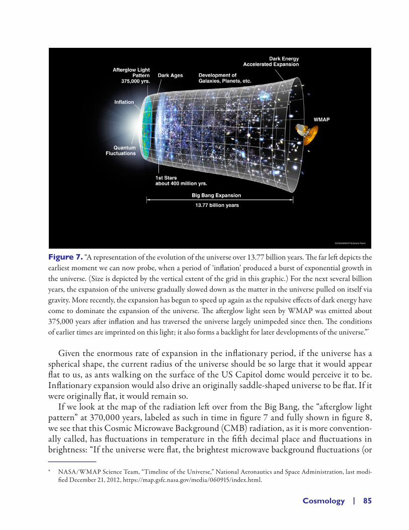
Cosmology | 85
Figure 7. “A representation of the evolution of the universe over 13.77 billion years. The far left depicts the earliest moment we can now probe, when a period of ‘inflation’ produced a burst of exponential growth in the universe. (Size is depicted by the vertical extent of the grid in this graphic.) For the next several billion years, the expansion of the universe gradually slowed down as the matter in the universe pulled on itself via gravity. More recently, the expansion has begun to speed up again as the repulsive effects of dark energy have come to dominate the expansion of the universe. The afterglow light seen by WMAP was emitted about 375,000 years after inflation and has traversed the universe largely unimpeded since then. The conditions of earlier times are imprinted on this light; it also forms a backlight for later developments of the universe.”*
Given the enormous rate of expansion in the inflationary period, if the universe has a spherical shape, the current radius of the universe should be so large that it would appear flat to us, as ants walking on the surface of the US Capitol dome would perceive it to be. Inflationary expansion would also drive an originally saddle- shaped universe to be flat. If it were originally flat, it would remain so.
If we look at the map of the radiation left over from the Big Bang, the “afterglow light pattern” at 370,000 years, labeled as such in time in figure 7 and fully shown in figure 8, we see that this Cosmic Microwave Background (CMB) radiation, as it is more convention-ally called, has fluctuations in temperature in the fifth decimal place and fluctuations in brightness: “If the universe were flat, the brightest microwave background fluctuations (or
* NASA/WMAP Science Team, “Timeline of the Universe,” National Aeronautics and Space Administration, last modi-fied December 21, 2012, https:// map .gsfc .nasa .gov/ media/ 060915/ index .html.

86 | Relativity Lite
‘spots’) would be about one degree across. If the universe were open, the spots would be less than one degree across. If the universe were closed, the brightest spots would be greater than one degree across.” WMAP has confirmed that the brightest spots are indeed about one degree across. As of 2013, WMAP tells us that “the universe is flat with only a 0.4% margin of error [and] that the Universe is much larger than the volume we can directly observe.”*
Figure 8. The Cosmic Microwave Background (CMB) radiation from nine years of WMAP data. The image shows temperature fluctuations on the Kelvin scale (above absolute zero) of up to ±0.0001 K around the average temperature of 2.7250 K. These are indicated from dark blue to red in the bar graph at right. The signal from our galaxy was subtracted off.†
Inflation also accounts for why regions of the universe far to the left and far to the right are at the same temperatures to five decimal places in figure 8. They are so far apart that energy in the form of light could not have traveled between them to equalize their temperatures within the 13.77 billion years WMAP data says is the age of the universe. However, their having nearly equal temperatures today would be what we would expect if their temperatures had been equalized when they were infinitesimal distances apart from each other in the early stages of universal expansion and then were flung far apart by inflation.
As a side note, it has been suggested that an inflationary expansion would magnify the spacetime foam shown in figure 11c of chapter 4 to such an extent that we should see huge voids of nothingness between today’s clusters of galaxies. Indeed, that is what Margaret J.
* NASA/WMAP Science Team, “Will the Universe Expand Forever?,” National Aeronautics and Space Administration, last modified January 24, 2014, https:// map .gsfc .nasa .gov/ universe/ uni _shape .html.
† NASA/WMAP Science Team, “CMB Images,” National Aeronautics and Space Administration, last modified April 14, 2014, https:// map .gsfc .nasa .gov/ media/ 121238/ index .html.

Cosmology | 87
Geller and John P. Huchra found by mapping the distribution of galaxies.* The reader may measure the red- shift velocities of some 200 galaxies in a telescope simulator called CLEA, available from Gettysburg College,† and plot this information against their angular posi-tions (called right ascension [RA] and equivalent to longitude on the Earth’s surface) in a small slice of the other angle (called declination [Dec.] and equivalent to latitude). Even with just 200 galaxies, the bubble structure is apparent, and it grows more marked with larger numbers of galaxies and adjacent declinations.
Those desiring to plot thousands of galaxies may access the Las Campanas Redshift Sur-vey Catalog,‡ the results of which are shown in figure 10. This is a composite of a trio of three- degree slices of the sky that one may see stacked not quite edge- on in figure 9 as red, green, and blue fans of galaxies.
Figure 9. Three slices of red- shift velocities of 4,000 galaxies at declinations from −46 to −43 degrees shown in blue, −43 to −41 in red, and −40 to −38 in green, seen almost edge on.
* M. J. Geller and J. P. Huchra, Science 246, 897 (1989).† The original Windows version is at http:// www3 .gettysburg .edu/ ~marschal/ clea/ univlab .html, and the version bottled
for Macintosh by Joel Cranston is at http:// archives .pdx .edu/ ds/ psu/ 15113.‡ In the search page at https:// heasarc .gsfc .nasa .gov/ db -perl/ W3Browse/ w3table .pl ?tablehead = name %3Dlcrscat & Action =
More +Options, one types “−46 .. −44” in the “dec” box and “> 1045” in the “radial velocity” box and hits “Start Search.” The automatic result is to limit the search to 1,000 galaxies. One may then change “Maximum Rows”: to “4,000” and hit the “Reissue Query” button. I changed the download from the default “Tabbed” to “Excel- compatible” and saved the file. I rearranged the columns so that “ra,” “dec,” and “radial_velocity” were in columns a, b, and c, and in cell K2 entered the equation “= “{“&RADIANS(A2)&”,”&C2&”},”.” I filled down to cell K4001 and copied the results into a Mathematica notebook. The four- term version would read “k45: = {{1.20937371982484,31150},{1.09713211922786,36760},{1.11332964735099,42616},{0.989954765988463,13140}},” where I have replaced the last comma with a curly bracket. The Math-ematica instruction, “ListPolarPlot[k45, PlotStyle −> Directive[PointSize[Tiny], Magnification −> 0.1, Blue]]” gives the blue plot.

Figure 10. Top view of a plot of the red- shift velocities of 4,000 galaxies against their right ascension (RA; equivalent to longitude on the Earth’s surface) for a thin slice of the other, declination, angle (equivalent to latitude) from −40 to −38 degrees, shown in green. An adjacent slice of another of 4,000 galaxies from −43 to −41 degrees is shown in red, and a third slice of another of 4,000 galaxies from −46 to −44 degrees is shown in blue. Not only do we see structures and voids across the face of the fan of galaxies (from RA 10 to 16 hours and from 10,000 to 80,000 km/s), but the structures and voids are shared to a significant degree among the three slices or the voids would have disappeared in this overlay. The galaxies, thus, appear to lie on surfaces akin to abutting soap bubbles.

Cosmology | 89
WHICH UNIVERSE DO WE LIVE IN?The debate for 75 years had been whether the universe would slow its expansion but con-tinue to expand forever or eventually stop and begin contracting into a Big Crunch. In 1998, two teams observing the brightness of distant Type Ia supernovae (stellar explosions of known intrinsic luminosity) independently determined that the expansion of the uni-verse is actually accelerating.* (The team leaders— Adam Riess, Brian Schmidt, and Saul Perlmutter— were awarded the 2011 Nobel Prize in Physics for their discovery.) See the right- hand side of figure 7.
What is causing this acceleration? This substance, which has to make up for 71.4% of the energy of the universe to account for current WMAP observations of the light left over from the Big Bang,† has been dubbed Dark Energy, but no one really knows what it is. Another 24% of the energy of the universe is dark matter, whose composition is likewise unknown and interacts with conventional matter (4.6% of the energy of the universe) only gravitationally.
Dark matter was first suggested by Fritz Zwicky as a way to explain the observed mo-tions of galaxies in the Coma cluster of galaxies: “[T]he average density in the Coma system would have to be at least 400 times greater than that derived on the basis of observations of luminous matter.”‡ Vera C. Rubin and W. Kent Ford’s measurement of the flat rota-tional speed curves of regions in the Andromeda Galaxy in 1970, and subsequently many other galaxies, provided sufficient evidence that dark matter extended far beyond the op-tically bright edge of galaxies to make the assumption of its existence the norm within astronomy.§
Figure 11 is a composite image: the Hubble space telescope was used to map the dark matter (colored in blue) using a technique known as gravitational lensing. Chandra X- ray Observatory’s data enabled the astronomers to accurately map the ordinary matter, mostly in the form of hot gas, which glows brightly in X- rays (shown in pink). It is significant that the blue lobes on either side, consisting of dark matter, have passed through the pink collision region with little to no interaction with the conventional matter. Indeed, there was little to no interaction with the oncoming dark matter from the other galaxy cluster other than the gravitational interaction that will eventually pull both ordinary matter and dark matter components into a rough ball in the central region.
* Adam G. Riess et al., Astron. J. 116, 1009 (1998), http:// iopscience .iop .org/ 1538 -3881/ 116/ 3/ 1009/ fulltext/; Astrophys. J. 517, 565 (1999), http:// iopscience .iop .org/ 0004 -637X/ 517/ 2/ 565/ fulltext/.
† NASA/WMAP Science Team, “Universe Content— WMAP 9yr Pie Chart,” National Aeronautics and Space Adminis-tration, last modified April 8, 2014, https:// map .gsfc .nasa .gov/ media/ 121236/ index .html.
‡ Fritz Zwicky, Helvetica Physica Acta 6, 110 (1933), with an English translation by Heinz Andernach at https:// arxiv .org/ abs/ 1711 .01693. See section 5.
§ Vera C. Rubin and W. Kent Ford Jr., Astrophys. J. 159, 379 (1970).

Figure 11. A collision of galaxy clusters, MACSJ0025.4- 1222, captured with the Hubble Space Telescope and NASA’s Chandra X- ray Observatory, provides striking evidence for dark matter and insight into its properties. The pink area is the normal matter from the collision of two galaxy clusters, heated up in the process of stopping much of each other’s forward momentum and therefore emitting X- rays captured by Chandra. The blue portions of this image map the mass required to account for gravitational lensing of light Hubble recorded from the distant objects by the cluster’s matter (dark and ordinary). The blue lobes on either side must therefore consist of dark matter that passed through the pink collision region with little to no interaction with the conventional matter nor with the oncoming dark matter from the other galaxy cluster. Credit: X- ray (NASA / CXC / Stanford / S. Allen); Optical/Lensing (NASA / STScI / UC Santa Barbara / M. Bradac)*
* NASA Science Team, “A Clash of Clusters Provides Another Clue to Dark Matter,” National Aeronautics and Space Administration, August 27, 2008, https:// www .nasa .gov/ mission _pages/ chandra/ multimedia/ photos08 -111 .html. See also the Bullet Cluster: “1E 0657- 56: NASA Finds Direct Proof of Dark Matter,” National Aeronautics and Space Admin-istration, last modified August 27, 2018, http:// chandra .harvard .edu/ photo/ 2006/ 1e0657/.

Cosmology | 91
One theory is that Dark Energy is what is known as the cosmological constant, a fudge factor Λ that Einstein added to his theory in 1917 to prevent an outward expansion and, thus, to match what nearly everyone believed was a static universe. He later told George Gamow “that the introduction of the cosmological term was the biggest blunder he ever made in his life.”*
There is a second Friedmann equation† that gives the acceleration, A, of the universe, defined as the change in the speed of expansion, S, with time,
AG
cp R= − +
43
32
π ρ (5)
where ρ is the conventional and dark matter density and p is the pressure of the universe. Einstein had wanted a static universe, one that did not change speed, so he would need A = 0. The most obvious ways one could do that is to have both ρ and p = 0 or R = 0. But the first idea is no good because this is a universe with nothing in it. The second is no better since it constitutes no universe to speak of. The better solution that apparently came to Einstein was to postulate a substance pervading the universe that has negative pressure of just the right size that the term in parentheses in equation (5) is 0. That is, at the present moment in time,
AG
cp R
Gc
c0 0 2 0 0 0 2 0
243
3 43
33
= − +
= − + −
π ρ π ρ ρ
=R0 0 (6)
This solution saw the light of day for only a few years before observations showed that the universe was expanding, undermining the need for a static solution.
Although this solution seems to do what Einstein wanted, it is highly unstable. If the universe were to shrink ever so slightly, the matter density would increase by a tiny fac-tor, but the negative pressure of the substance pervading all space would not change. This increase in the matter density would pull the matter further inward, again increasing the matter density, and so on, and one would ultimately have a runaway collapse of the universe.
Or if the universe were to expand ever so slightly, the matter density would decrease by a tiny factor but the negative pressure of the substance pervading all space would not change. This disbursement of the matter to a larger volume would have less of an inward gravitational tug, allowing the matter to move farther apart, again decreasing the matter density, and so on, and one would ultimately have a runaway expansion of the universe. Al-though this instability would have proved a disaster for Einstein’s attempt at finding a static solution for the universe, it is just what one needs for a runaway expansion of the universe like that observed in 1998.
In this case, we want a version of equation (6) whose acceleration, radius, and mass density can change with time. Also, the negative pressure (the interior parenthesis on the
* George Gamow, My World Line, an Informal Autobiography (Viking Press, New York, 1970), p. 44.† Tai L. Chow, Gravity, Black Holes, and the Very Early Universe an Introduction to General Relativity and Cosmology
(Springer, New York, 2008), p. 142, eq. (8.36– 37).

92 | Relativity Lite
right- hand side of equation [6]) is more conventionally written in terms of the cosmological constant, Λ, so we transform equation (6) to read
AG
RG
RG
R R= − + ≡ − +4
34
34
3 30π ρ π ρ π ρ Λ
(7)
The required “substance” with negative pressure could simply be the vacuum energy of “empty” space Casimir’s work led us to.
This adds a new term to equation (4a), the first Friedmann equation that gives the expan-sion velocity of the universe:
S2/c2 = Rmax/R − k + 1/3 Λ R2/c2 (8a)
One sees that early enough in the expansion of the universe, R is small, and its square is smaller still, so that Λ will have no discernible effect. But eventually, R will get big enough and its square will drive the expansion speed S to larger and larger values. This first Fried-mann equation, too, gives a runaway acceleration of the universe that is just starting in the visualization equation (8b) with k = 1,
(8b)
There are candidates for what is driving the acceleration of the universe other than the vacuum energy of “empty” space, and there also are some unresolved problems with calcu-lating the vacuum energy density. See, for instance, the work of Robert Caldwell, Rahul Dave, and Paul Steinhardt on a form of dark energy called “quintessence.”* We will leave readers to explore such on their own— after, of course, listening to some more music, say Youssou N’Dour’s song “Liggey” (Live In London, 2003).
* R. R. Caldwell, R. Dave, and P. J. Steinhardt, Phys. Rev. Lett. 80 (8), 1582– 85 (1998).

Appendix | 93
APPENDIX
For the Instructor’s Use
An appendix fi lled with nonstop mathematical gore may seem like a strange tag onto a book intended to teach people about relativity using primarily pictures, containing only as many equations as are absolutely required. I nevertheless include it for instructors and those few readers who do not mind the math. I do so for three reasons. First, an arc- length claim is made in chapter 4 of this book that is given without visual proof, and readers might wish to know that such a proof exists. Second, one may want to determine time- dilation factors exactly for the accelerated portions of our trip to Alpha Centauri in chapter 3. Th ird, refer-ences that lay out relativistic relations that include acceleration without tensor analysis are almost nonexistent. An out- of- print book by Francis Sears and Robert Brehme* is the only one I have found.
To show that the arc length in fi gure 10 of chapter 4 is given by equation
τ 22
21 2= −
Arc
t , (A1)
(where A = GM/r2) and, ultimately, to get the Schwarzschild radius, one must fi rst know the relations between position, coordinate time, and proper time in an accelerated system. One fi rst correctly defi nes acceleration in terms of proper- time derivatives of the four- velocity,
X ct rµ = { }, , (A2a)
VdXd
V V cdrdt r
µµ
τγ
τ= = { } =
, ,
, (A2b)
where the superscript μ takes the values 0, 1, 2, and 3 referring to time and the three spatial coordinates. Notice that V is the derivative of position X with respect to the proper time and whose proper time derivative is the acceleration:
AdVd
A At rµ
µ
τ= = { },
. (A2c)
* F. W. Sears and R. W. Brehme, Introduction to the Th eory of Relativity (Addison- Wesley, Reading, MA, 1968), p. 102 ff .

94 | Appendix
We also note that
vdrdt
= (A2d)
and
γτ
=dtd
. (A2e)
c/γ
c
v
c
V
Vt
θ
θv γ/c 2
r
Figure 1. Equations (A3a, b). Graphical depiction of relationships among invariant, spatial, and temporal components of various four- vectors.
Now, from the Pythagorean theorem applied to the upper triangle in figure 1, or using the definition of the proper- time interval for a flat metric,
ηµν = −−
−
1 0 0 00 1 0 00 0 1 00 0 0 1
(with the Einstein convention that repeated indices imply a sum over all possible values),
c d dX dX dX dX c dt dr c v dt2 2 2 2 2 2 2 2τ ηµµ
µνµ ν≡ = − = −( )= . (A3a)
Then dividing by dτ2,
c V Vt r2 2 2= − (A3b)

Appendix | 95
shows that the lower triangle in figure 1 is similar to the upper triangle. Finally, the τ deriv-ative of (A3b) gives
0 = − =V A V A V At t r r µµ . (A3c)
In the instantaneous rest frame of the uniformly accelerating rocket, Vr = 0 and Vt = c so that the angle θ in figure 1 goes to 0. In this case, (A3c) implies At = 0. Then the spatial part of the acceleration four- vector in the instantaneous rest frame of the rocket (with θ = 0 in figure 2, the triangle equivalent to figure 1 for acceleration) gives the size of the invariant acceleration, A Ar
2 2= , just as the temporal part of the momentum four- vector in the instan-taneous rest frame of the rocket gives the invariant mass, E mc0
2= . A vector with the former properties is called space- like, and those with the latter (more conventional) properties are called time- like. This means that for θ > 0, figure 2 must have Ar on the hypotenuse.
Then this triangle is similar to the one for velocity only if the three- acceleration is parallel to the three- velocity. All the following assumes this restriction. We take both three- acceleration and three- velocity parallel to the x- direction for simplicity; then, from (A3c), A V A Vt t x x= . From figures 1 and 2,
sin / / /θ = = =v c V V A Ax t t x , (A4a)
cos / / /θ γ= = =1 c V A At x , (A4b)
tan / / /θ γ= = =v c V c A Ax t . (A4c)
A A
A
θ
t
r
Ar
Figure 2. Equations (A4a– c).
From sec tan2 2 1θ θ− = , one may show that
A A V cx x= +1 2( / ) (A5a)
or
dVV c
A dx
x1 2+=
( / )τ . (A5b)

96 | Appendix
Since c and A are invariant constants, one may integrate* to obtain
V c A c V cx x= + ( ) sinh /τ arcsinh 0 , (A6)
where we have set τ0 = 0, and Vx(τ = τ0 = 0) = Vx0. We integrate again† to obtain
X X cA
A c V c V cx x x x− = + ( )[ ] − +
0
2
0 02 21cosh /τ arcsinh , (A7)
where we have used arcsinh arccoshy y( ) = +( )1 2 . Using (A6) in (A5a),
A A A c V cx x= + ( ) cosh /τ arcsinh 0 . (A8)
Dividing (A6) by (A8) and using (A4c) and (A4b), we have
v c A c V cx= + ( ) tanh /τ arcsinh 0 . (A9a)
Now using (A2e) and (A4b) in (A8) and integrating
dt d d A c V c dx= = = + ( ) γ τ τ τ τsec cosh /Θ arcsinh 0 (A10)
yields
tcA
A c V c V cx x= + ( ) −( )sinh /τ arcsinh 0 0 , (A11)
where we have synchronized clocks at t0 = τ0 = 0. Note that this is not γ τ: it is only for differentials (dt = γ dτ) where this is true for accelerated systems. For extended durations, one must use (A11) and its inverse relation,
τ =+
−
cA
At Vc
cA
Vc
x xarcsinh arcsinh0 0 . (A11a)
Also note that the limit is
tVcA
x→ +→0
02
21 τ . (A11b)
Inverting (A9a) gives
V cAc
vcx0 = − +
sinh τ arctanh (A9b)
* I. S. Gradshteyn and I. M. Ryzhik, Table of Integrals, Series, and Products (Academic, New York, 1980), p. 99, No. 2.261(b).† I. S. Gradshteyn and I. M. Ryzhik, Table of Integrals, Series, and Products (Academic, New York, 1980), p. 155, No. 2.248.1.
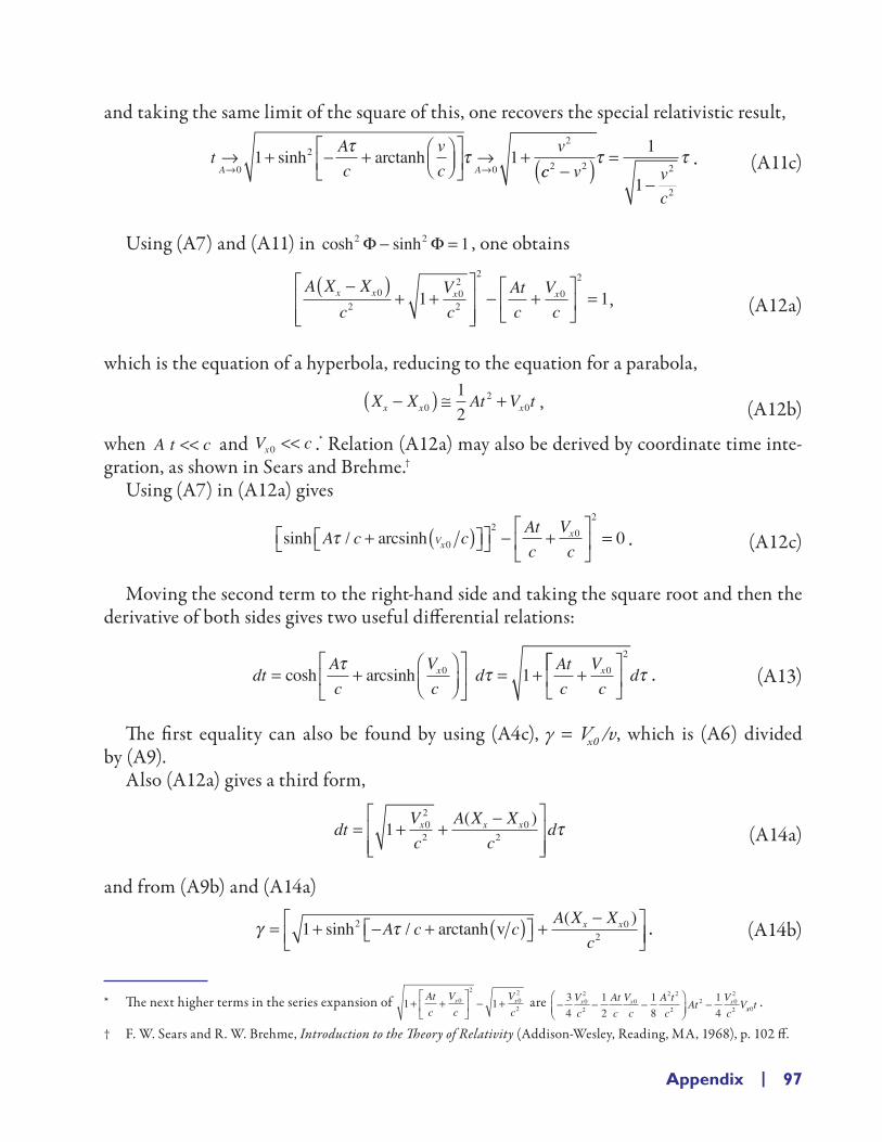
Appendix | 97
and taking the same limit of the square of this, one recovers the special relativistic result,
tAc
vc
vA A→ + − +
→ +→ →0
2
0
2
1 1sinh τ τarctanhcc v v
c
2 2 2
2
1
1−( ) =
−τ τ . (A11c)
Using (A7) and (A11) in cosh sinh2 2 1Φ Φ− = , one obtains
A X X
cVc
Atc
Vc
x x x x−( )+ +
− +
=0
202
2
2
02
1 1, (A12a)
which is the equation of a hyperbola, reducing to the equation for a parabola,
X X At V tx x x−( ) ≅ +02
012
, (A12b)
when A t c<< and V cx0 << .* Relation (A12a) may also be derived by coordinate time inte-gration, as shown in Sears and Brehme.†
Using (A7) in (A12a) gives
sinh /A c cAtc
Vc
Vxxτ + ( ) − +
arcsinh 0
2 02
== 0 . (A12c)
Moving the second term to the right- hand side and taking the square root and then the derivative of both sides gives two useful differential relations:
dtAc
Vc
dAtc
Vc
x x= +
= + +cosh τ τarcsinh 0 01
2
dτ . (A13)
The first equality can also be found by using (A4c), γ = Vx0 /v, which is (A6) divided by (A9).
Also (A12a) gives a third form,
dtVc
A X Xc
dx x x= + +−
1 02
20
2
( ) τ (A14a)
and from (A9b) and (A14a)
γ τ= + − + ( ) +−
1 2 02sinh / ( )
A c cA X X
cx xarctanh v . (A14b)
* The next higher terms in the series expansion of 1 102
02
2+ +
− +
Atc
Vc
Vc
x x are − − −
−34
12
18
14
02
20
2 2
22 0
2
2
Vc
Atc
Vc
A tc
AtVc
Vx x xxx t0
.
† F. W. Sears and R. W. Brehme, Introduction to the Theory of Relativity (Addison- Wesley, Reading, MA, 1968), p. 102 ff.

98 | Appendix
For small A, this simplifies to
γ τ→−
+ − −−
→A
x x
vc
A X Xc v
c
vc0 2
2
02 2
2
21
1
1
1
( ), (A14c)
which reduces to the nonaccelerated value for A = 0.Upon inverting (A13) and expanding the denominator in a series, one obtains
dA X X
cVc
A X Xc
Vx x x x x xτ( ) = −−( )
− +−( )
+2 02
02
20
202
12
3 12 cc
Vc
dtx2
2
04
421
4
+ +
( )... , (A15a)
of which (A1) is the first approximation if Vx0 = 0. Note that with A = 0, one regains the special- relativistic equation for time dilation at constant velocity Vx0 (which equals v0 in lowest order).
Finally, we note that the uniform acceleration of the rocket in the same direction as the change in position, as in figure 2a of chapter 4, feels like (is equivalent to) gravitational acceleration in the opposite direction to the change in position in figure 2b of chapter 4. So we replace
A x A rFm
rV r
mGM
rthrusters gravityg∆ ∆ ∆⇒ − = − = − =( ) ( )1 2 (A16)
to give* the Schwarzschild solution of chapter 4,
t
rGMc
2
2
21
1 1 2=− ×
τ . (A15b)
Alternatively, one can prove that the arc in figure 10 of chapter 4 really has length
c tA xc
c∆∆
∆= +
1 2 τ . (A17)
The relations derived above are necessary for this second proof. The arc- length is defined parametrically by
L c
dxcd
dtd
d
cA
=′
+′
′
= +
∫ τ ττ
τ
τ 2 2
2
0
1 2sinhcc
d
∫ ′
0
τ
τ . (A18)
* To obtain this from the above expression, we first redefine our distance coordinate as decreasing downward rather increas-ing downward as above, by changing the sign of all r’s. Next we note that m A r is just the gravitational potential energy −G m M/r.

Appendix | 99
where we have set Vx0 = 0.As with elliptical integrals, one expands the radical in the small parameter A τ/c and uses
(A7) and (A11) to obtain
L cAc
d
ccA
= +′
+ ⋅ ⋅ ⋅
′
= +
∫ 1
2
2
0
sinh
si
τ τ
τ
τ
nnh coshAc
Ac
c
τ τ τ
τ
− + ⋅ ⋅ ⋅
=
12
2++ − +
cA
Ac
Ac
2
21 1sinh coshτ τ
+ ⋅ ⋅ ⋅
= +−
+
+ ⋅ ⋅ ⋅c ct A x x
cτ2 2
102
( ) ,
(A19a)
where we have set Xx = x and Xx0 = x0 for a more conventional notation.Finally, suppose the length of this arc is L = c t to first approximation, as labeled in
figure 10 of chapter 4; then (A19a) becomes
ct
A x xc
c1 12
12
02−−
+
+ ⋅ ⋅ ⋅
=( ) τ
(A19b)
or
tA x x
c1 0
2−−
+ ⋅ ⋅ ⋅
=( ) τ , (A19c)
giving (A14a) to first approximation. Thus, the assumption L = c t is a consistent one, show-ing that the gravitational red- shift factor is essentially just the stretched path- length for a beam of light in a gravitational field.
Finally, one may want a relation like (A12a) involving just position and velocity, which may be obtained by solving (A7) and (A9) using the relation cosh sinh2 2 1Φ Φ− = ,
vV A x x V
cA x x
c
c V
xx
x
202
002
20
2
202
2 1=
+ − + + −
+
( ) ( )
++ − + + −
−
→→
2 1
2
002
20
22
00A x x Vc
A x xc
cA x x
x V( ) ( )
( 000
2
20
02
2
) ( )
( ) ( )
+ −
+ − + −
A x xc
c A x x A x xc
c22.
(A20a)
When A is small, this reduces to the nonrelativistic form for constant A:
12
202
0v v vdv Adx A x x−( ) = = = −∫ ∫ ( ). (A20b)
It is generally more convenient to calculate v from A via the relation (A13):
dtVc
A x xc
d dvc
dx= + +−
≡ ≡−
1 1
1
02
20
2 2
2
( ) τ γ τ τ , (A21)

100 | Appendix
or
v c cVc
A x xc
cx
≡ − = −
+ + −
≅ −
+
1 1 1 1
1
1 1
12
02
20
2
2γ ( ) AA x xc
Vc
x( )− +
02
02
2
212
.
(A22)
Then we can rewrite (A12a) as
Atc
Vcx+
= −0
22 1γ ,
(A23a)
or
t
cA
Vcx= − −
γ 2 01 .
(A23b)
We can obtain the corresponding relation between distance and γ by solving (A21) for x − x0, which we also called r in chapter 3.
r x x
cA
Vc
x≡ − = − +
( )0
202
21γ .
(A24)
INITIAL ACCELERATION TOWARDS ALPHA CENTAURILet us use these to find how long it takes to boost a rocket to v = 0.6 c (γ = 1.25) at an acceleration of 1 g.* If the initial velocity with Vx0 = 0, we have from (A23b) t = 0.726536 yr. Likewise (A24) gives the distance traveled when this speed is reached, r = 0.242179 c yr.
Inverting (A9a),
τ =
+
cA
Vc
vc
x-arcsinh arctanh0
(A9c)
gives τ = 0.671462 yr, as does inverting (A11a),
τ =
+
−
cA
At Vc
Vc
x xarcsinh arcsinh0 0 .
(A11d)
We can use this to confirm the caution after equation (A11) that for extended periods of
acceleration, the ratio t/τ = 1.08 is indeed not γ = 1.25 even though we still have v c= −1 12γ
if γ is defined as in equation (A22).
* A 1 g acceleration can be written in the useful form A/c = 1/(0.968715 yr).

Appendix | 101
CONTINUOUS ACCELERATION TO CYGNUS X- 1Suppose we want to travel out to the black hole Cygnus X- 1, 7,733 light- years away* in the shortest reasonable time. The rocket would accelerate at 1 g for half the trip, flip over and decelerate at 1 g for the remainder of the trip. At this acceleration, the rocket will reach the halfway point with a time- dilation factor given by (A21) of
γ = + +−
= +1 1 10 98715
386602
20V
cAc
x xc yr
x ( ).
( .55 0cyrc
−
),
or γ = 3,992.37. Equation (A22) gives the rocket’s velocity as it just reaches the halfway
point, r = 3,866.5 c yr, as v c= −1 12γ
= 0.99999997 c. Equation (A23b), with Vx0 = 0,
gives the time for the half trip at tcA
= −γ 2 1 = 3,867.47 yr, where we use the Julian year of
365.25 days as preferred by the IAU.† Both equations (A9c) and (A11d) give τ = 8.70418 yr.In chapter 4, we said that under large acceleration, “figure 1c will stretch out as in
figure 1d, so much so that the curved light path will differ little from the straight hypot-enuse. Both high constant speeds and large accelerations (to high speeds) give enormous time dilation.” We can now quantify these two claims in the present case of 1 g accelera-tion. The hypotenuse of the triangle under the hyperbolic curve shown in figure 1d, whose legs are r and c τ (as calculated above using the correct formula for acceleration [A9c] or [A11d]), is c t' = 3,866.51 c yr, just under 1 light- year shorter than the hyperbola, whose length is c t = 3,867.47 yr, a 0.02 % difference.
The intermediate constant velocity that would give such a triangle is r/t = 0.999997 c, indeed a high constant speed, differing in the sixth decimal place from the rocket’s veloc-ity as it just reaches the halfway point. It would give a very big time dilation factor when calculated in the special- relativistic manner: t'/ τ = 444. But the frame- shifting a rocket undergoes when accelerated at 1 g leads to a time dilation factor nearly ten times larger, γ = 3,992.37 when calculated using the correct (and consistent) formula for acceleration (A21). We see that our intuitive connection between the two cases falls well short of the reality, a divergence that will only grow as we go to even larger accelerations (to much higher speeds).
* The 2018 Gaia DR2 catalogue shows a parallax of 0.4218 mas, which gives d = 1/0.0004218 = 2371 pc = 7733 c yr. “DR22059383668236814720,” Centre de Données astronomiques de Strasbourg, last modified May 26, 2020, http://simbad.u-strasbg.fr/simbad/sim-id?mescat.distance=on&Ident=%402905066&Name=DR2+2059383668236814720&submit=display+all+measurements#lab_meas. Other names one can use for the searchinclude HD 226868 and 1956+350.
† G. A. Wilkinson, IAU Style Manual Comm. 5, in IAU Transactions XXB (unpublished pamphlet), 1987, p. S23, https://www.iau.org/static/publications/stylemanual1989.pdf (accessed June 26, 2020); https://www.iau.org/publications/proceedings_rules/units/ (accessed June 26, 2020).


Index | 103
INDEX
1g (see one gravity)2D, 47, 64
abbreviated, 25, 26Abell 2218, 48absolute zero, 68, 86accelerating expansion, 71, 84acceleration, 25, 26, 36, 37, 38, 39, 41, 43, 44, 45,
56, 60, 89, 91, 92, 93, 95, 98, 101age of the universe, 86Albrecht, Andreas, and Paul J. Steinhardt, 80, 83Alpha Centauri, 28, 29, 30, 31, 32, 33, 34, 36, 37,
38, 39, 93, 100Alpher, R. A., and R. C. Herman, 68Andromeda Galaxy, 89angular momentum, 52, 53, 81annihilating, 80antigravitational force, 84antimatter, 80, 82antiprotons, 80approxiamations, 23arc, 29, 45, 47, 48, 49, 53, 56, 72, 73, 93, 98, 99astronaut, 24, 45, 59, 61, 62, 63atmosphere, 8, 9, 10, 18, 28, 50, 55
back in time, 77backward, 71, 76, 78ball, 24, 25, 45, 47, 82, 83, 89balloon, 68, 74Barish, Barry, Kip Thorne, and Rainer Weiss, 66barrier, 52, 53beam of light, 2, 5, 45bending, 46, 47, 48, 50, 52, 56, 60, 64
Big Bang, 67, 68, 77, 79, 84, 85Big Crunch, 77, 89black hole, 59, 60, 61, 63, 64, 65,
66, 101blue shift, 32boundless, 74Brunelleschi, Filippo, 46
c (the speed of light), 3, 4, 5, 6, 7, 8, 9, 10, 12, 13, 14, 15, 16, 18, 19, 20, 21, 22, 24, 25, 26, 27, 28, 29, 30, 32, 33, 34, 36, 37, 38, 44, 45, 58, 60, 61, 62, 75, 80, 87, 95, 96, 99, 101
Caldwell, R. R., R. Dave, and P. J. Steinhardt, 92Cameron, Alastair, 67carbon, 50, 54Casimir, Hendrik, 81, 92Chandra telescope, 89, 90Chandrasekhar, Subrahmanyan, 55chord, 72, 73circumference, 70, 72, 73classical, 61CLEA, 87clock, 2, 3, 4, 5, 12, 15, 23, 24, 34, 35, 37, 41, 56,
61, 63, 69, 70, 72, 73, 96clocks running slowly, 41closed universe, 77, 78, 86cluster, 48, 89, 90CMB (see Cosmic Microwave Background)coalescence, 54coincident, 31collapse, 54, 55, 56, 62, 63, 77, 91collide, 65Coma cluster, 89

104 | Index
comets, 57conservation laws, 81Conservation of Energy, 50, 57, 81constant speed, 43conventional matter, 89, 90convert, 65coordinate time, 5, 12, 29, 45, 60, 68Copernican, 15core of the star, 54Cosmic Microwave Background (CMB),
85, 86cosmic scale factor (R), 14, 51, 52, 53, 54, 65, 67,
68, 72, 73, 74, 75, 77, 79, 91, 92, 93, 97cosmological constant (Lambda, Λ), 67, 89,
91, 92Cranston, Joel, 87critical, 74, 77Curie temperature, 81, 82curvature parameter (see k)curve, 26, 44, 45, 46, 47, 51, 52, 53, 59, 64, 72, 73,
75, 77, 82, 89, 101Cygnus X- 1, 101
dark energy, 92dark matter, 89, 90de Sitter, Willem, 67Dec. (see Declination)deceleration, 38, 39, 40Declination (Dec.), 66, 87degeneracy force, 54, 55degenerate state, 54density, 54, 67, 74, 75, 76, 77, 78, 80, 83, 84, 89,
91, 92detect, 65deuteron, 28, 54diagram, 49, 51, 52, 53, 59, 84dilated (see also time dilation), 5, 10, 15, 18, 37,
45, 59dimples, 47disk, 47, 69distance, 3, 4, 5, 6, 15, 16, 18, 19, 24, 29, 32, 34,
36, 37, 38, 39, 45, 51, 53, 56, 58, 59, 60, 61, 66, 67, 68, 69, 70, 71, 72, 73, 80, 81, 98
dose of radiation, 10Dunn, L. C., and Th. Dobzhansky, 11duration, 24, 37
dust, 54Dyson, F. W., A. S. Eddington, and
C. Davidson, 48
Earth, 2, 3, 4, 5, 8, 9, 12, 13, 15, 16, 18, 24, 28, 29, 30, 31, 32, 33, 34, 35, 36, 37, 38, 39, 40, 47, 48, 49, 54, 55, 57, 58, 59, 60, 61, 68, 87, 88
Earth Gravity, 38Earth- pulse, 36Einstein, Albert, 2, 14, 18, 19, 23, 26, 27, 35, 43, 45,
48, 49, 53, 56, 58, 61, 63, 64, 67, 83, 91, 94electric and magnetic fields, 83electron, 38, 54, 80, 82, 83electron Volt, 28elliptical, 52, 53, 57, 99emitted, 4, 15, 16, 30, 31, 32, 33, 34, 35, 36, 37, 39,
61, 65, 85emptiness, 71, 80empty, 80, 81, 92energy, 3, 13, 19, 24, 25, 27, 28, 49, 50, 51, 52,
53, 54, 57, 65, 80, 81, 82, 83, 84, 85, 86, 89, 92, 98
Englert, Francois, and Robert Brout, 79equalized, 86equilateral triangle, 73escape, 58ether, 2eV, 28expanding, 34, 35, 64, 65, 67, 69, 70, 71, 72, 75, 76,
78, 84, 91, 98expansion, 68, 71, 72, 73, 74, 75, 77, 78, 80, 84, 85,
86, 89, 91, 92, 97exploded, 13, 77exponential growth, 85extragalactic, 67
false vacuum, 83, 84flat, 63, 74, 77, 85, 89, 94floor, 24, 38fluctuations, 85, 86flying saucer (see saucer)force, 12, 13, 24, 38, 43, 49, 51, 52, 53, 54, 55, 62,
71, 75, 77, 80, 83, 84four- dimensional, 24, 25, 26, 27four- dimensionality, 46frame of view, 77

Index | 105
frame shifting, 37frame to frame, 39free space, 43, 61frequency, 30, 32, 33, 35, 37, 61friction, 76, 82Friedmann equation, 74, 91, 92funnel, 49, 51, 55, 83fuse, 54future, 64, 71, 78
G. Douglas Straton, 11, 12Gaia telescope, 29galactic cluster, 48galaxy, 48, 67, 69, 70, 71, 72, 73, 76, 77, 78, 86, 87,
88, 89, 90gamma (γ) (see time dilation)Gamow, George, 91Geller, Margaret J., and John P. Huchra, 87graphic calculator, 19graphically, 45gravitational, 25, 43, 45, 49, 51, 53, 54, 55, 56, 57,
60, 63, 64, 65, 66, 68, 71, 74, 77, 80, 83, 84, 89, 90, 91, 98, 99
gravitational field, 45, 57, 63, 68, 99gravitational wave, 64, 65gravitationally, 38, 46, 48, 61, 89grid, 30, 32, 33, 34, 39, 40, 47, 85ground state, 82Guth, Alan H., 79, 80, 83, 84
H0 (Hubble constant), 73, 74, 77Hagen, Carl, Gerald Guralnik, and Tom Kibble, 79half- life, 8, 9, 10, 18, 26Hanford LIGO, 65, 66heat, 54, 83height, 3, 6, 9, 24, 57Heisenberg’s uncertainty principle, 80helium, 54, 67helium flash, 54Higgs, Peter W., 13, 28, 79, 80, 81, 83, 84Higgs boson, 13, 28, 79Higgs false vacuum, 84Higgs field, 79, 80, 84high- temperature, 82, 83Hilbert, David, 78, 79homogeneous, 71
hot, 54, 76, 77, 80, 83, 89Hubble, Edwin, 67Hubble Space telescope, 89, 90Hubble– Lemaître law, 67, 69, 70, 71, 73,
74, 75Hulse, Russell, and Joseph Taylor Jr., 65hydrogen, 28, 54, 67hypersphere, 68, 71, 74hypotenuse, 5, 18, 19, 21, 22, 26, 27, 28, 44, 45,
60, 95, 101
IAU, 67, 101ice skater, 52, 81illusion, 38inertia, 51, 53infinite, 12, 13, 55, 56, 57, 60, 61, 63, 74,
76, 77, 78infinitely, 55, 59, 60, 67, 77, 78, 79infinitesimal angle, 81infinity, 13, 57, 58, 60, 78, 79inflation, 79, 84, 85, 86inflationary expansion, 80, 84, 85, 86interstellar shock wave, 54invariant, 13, 26, 27, 28, 94, 95, 96iron, 54, 81Israel, Werner, and Eric Poisson, 62
k (curvature parameter), 74, 75, 76, 77, 78, 92KE (see kinetic energy)Kelvin, 86Kerr Black Holes, 63Kervella, P., F. Mignard, A. Mérand, and F.
Thévenin, 29kinetic energy (KE), 24, 27, 28, 50, 51, 57, 81koan, 13
Lagrangian, 81Lamoreaux, S. K., 81Las Campanas Redshift Survey Catalog, 87Latitude, 87, 88Led Zeppelin, 23Lemaître, Georges, 67, 69, 70, 71, 73, 74length, 5, 6, 15, 18, 19, 24, 26, 27, 34, 45, 56, 59,
60, 62, 69, 72, 73, 93, 95, 98, 99length contraction, 18, 34life, 10, 11, 12, 14, 25, 91

106 | Index
light, 2, 3, 4, 5, 6, 7, 12, 13, 15, 16, 18, 23, 26, 28, 29, 30, 32, 34, 35, 36, 37, 39, 40, 43, 44, 45, 46, 47, 48, 49, 55, 56, 58, 60, 61, 65, 66, 68, 74, 80, 85, 86, 89, 90, 91, 99, 101
light pulses, 29, 30, 32, 33, 34, 35, 37, 39, 40LightSail 2, 28LIGO, 65, 66limit, 12, 13, 14, 43, 49, 60, 87, 96, 97Linde, Andrei, 80, 83Livingston LIGO, 65, 66Lloyd, Charles, 19Longitude, 87, 88
MACSJ0025.4– 1222, 90magnet, 81, 82, 83magnetic moment, 82magnetization, 81, 82, 83marble, 50, 51, 53, 57, 81mass, 13, 14, 19, 25, 26, 28, 38, 47, 48, 54, 55, 56,
58, 60, 61, 63, 65, 66, 67, 71, 75, 77, 81, 83, 90, 91, 95
massive, 28, 48, 49, 54, 55, 64, 65, 79massless, 28, 67, 79, 80matter, 2, 3, 26, 54, 74, 76, 77, 85, 89, 90, 91measurement, 6, 24, 29, 89Mercury, 47, 49, 51, 52, 53MeV, 28mirror, 4, 16, 23, 82mirrors, 3, 4, 15Mitchell, John, 59momentum, 14, 24, 25, 27, 28, 38, 49, 52, 53, 63,
77, 80, 81, 90, 95Moon, 3motion, 2, 6, 18, 24, 26, 29, 34, 38, 45, 49, 50, 51,
52, 53, 62, 64, 73, 82movie, 37, 39, 40, 57, 76muon, 8, 9, 10, 18, 26, 28music, 19, 23, 92mutation, 11
N’Dour, Youssou, 92nebulæ, 67negative pressure, 84, 91neon, 54neutrino, 54neutron, 54, 55
neutron star, 54Newton, Isaac, 49, 50, 56, 74Newtonian, 27, 50, 51, 52, 53, 59, 77, 83, 84Nobel Prize, 65, 66, 79, 89Noether, Emmy, 81noise, 66nonexistence, 71North, 24, 46, 51, 82Northward momentum, 25nuclear fusion, 54nuclei, 54, 67nucleus, 28, 54
observatories, 66Occam’s razor, 14omnipotent observer, 29, 35omniscient perspective, 36omniscient view, 30one gravity (1g), 38, 101one- dimensional, 24, 26one- way membrane, 63onion, 54open universe, 77, 86orbit, 49, 51, 52, 53, 55, 56orbital, 52orbits, 49, 57orbs, 47oscillations, 83, 84oscillatory motion, 82oxygen, 54
paradox, 37, 41parallax, 29, 101parallax arc- seconds, 29parity, 82parsecs, 29, 67particles, 8, 28, 76, 79, 80, 83, 84PE (see potential energy)Penzias, A. A., and R. W. Wilson, 68perihelion, 49, 53, 57Perlmutter, S., 89perpendicular, 3, 21, 24perspective shift, 39perturbation, 83photon, 28, 45, 58, 83piston, 83, 84

Index | 107
planets, 35, 37, 49, 51, 52, 53, 54, 55, 56, 57plasticity, 11popcorn, 83positrons, 80potential energy (PE), 25, 49, 50, 51, 53, 57, 82precession, 53pressure, 54, 77, 80, 83, 84, 91, 92principle of equivalence, 38, 45, 46probabilistic, 63proper time, 5, 12, 13, 18, 26, 37, 45, 60, 68, 93protons, 28, 54, 61, 66, 80pseudoforce, 51Ptolemaic, 2, 15pulse, 29, 30, 31, 32, 33, 34, 35, 36, 37, 39, 40Pythagorean theorem, 5, 21, 22, 28, 59, 68
quantum, 54, 55, 61, 62, 80, 83
R (see cosmic scale factor)RA (see Right Ascension)radial, 53, 68, 87radiation, 3, 10, 12, 13, 61, 65, 68, 80, 85, 86radiation dosage, 10radius, 10, 19, 51, 52, 56, 58, 59, 60, 63, 68, 69, 70,
71, 72, 73, 75, 78, 85, 91reality shift, 38recessional velocities, 67, 70, 72, 73recipe, 22red shift, 32, 87, 88reference, 2, 4, 5, 12, 18, 23, 26, 29, 34, 36, 37,
39, 43reference frame, 4, 37relativistic Doppler shift, 32, 40relativistically, 14RelLab, 29, 30, 34, 38, 39rest, 8, 13, 15, 16, 18, 23, 26, 27, 28, 29, 34, 35, 36,
37, 39, 50, 57, 60, 71, 82, 83, 95rest mass, 13Riess, Adam G., 89Right Ascension (RA), 87, 88ring, 30, 35, 63, 77Rmax, 74, 75, 92Robertson, H. P., and A. G. Walker, 67Robertson- Walker metric, 68, 74rocket, 12, 13, 14, 15, 16, 18, 23, 24, 26, 27, 38, 60,
68, 95, 98, 101
rotational, 63, 82, 89Rubin, Vera C., and W. Kent Ford, 89rugby, 24, 25runaway expansion, 84, 91
saddle shape, 74, 77Sakurai Prize, 79saucer, 29, 30, 31, 32, 33, 34, 35, 36, 37, 38, 39, 40scale, 38, 47, 69, 71, 72, 74, 77, 86Schwarzschild radius, 56, 59, 60, 61Schwarzschild solution, 93, 98Sears, F. W., and R. W. Brehme, 93shape, 22, 27, 45, 68, 74, 76, 77, 82, 83, 85, 86similar triangles, 22, 27simultaneous, 23singularity, 56, 61, 62, 63, 77soap bubbles, 88solar masses, 65, 66Solar System, 15, 57space, 3, 4, 5, 6, 7, 13, 15, 16, 24, 25, 26, 28, 29, 30,
32, 43, 45, 46, 47, 51, 54, 55, 56, 61, 62, 63, 64, 67, 68, 74, 79, 80, 81, 89, 91, 92, 95
spacecraft, 28, 44spaceship, 3, 4, 5, 6, 7, 13, 15, 16, 28, 32, 43, 45, 46,
56, 61spacetime, 24, 47, 48, 49, 50, 51, 53, 55, 60, 61, 63,
64, 65, 68, 69, 74, 76, 80, 83, 84, 86spatial, 46, 64, 65, 68, 69, 70, 71, 93, 94, 95spectrum, 3, 30, 32speed, 2, 3, 4, 5, 6, 7, 9, 12, 13, 14, 18, 21, 23, 25,
26, 28, 30, 36, 38, 39, 43, 50, 57, 58, 60, 63, 65, 66, 68, 71, 72, 73, 74, 81, 85, 89, 91, 92
speed of light, 2, 3, 5, 13, 43, 60sphere, 69, 70, 71, 72, 74, 77, 78spherical, 63, 71, 72, 77, 85spin, 52, 61, 63, 79, 81spiral, 65spiritual meaning, 11spontaneously broken, 82star, 29, 32, 47, 48, 54, 55, 56, 60, 61, 62, 63, 64, 65,
83, 84, 101static, 67, 91stellar, 54, 89Straton, G. Douglas, 11, 12Sun, 28, 29, 30, 34, 36, 47, 49, 51, 53, 54, 57,
58, 59
108 | Index
supernova, 54, 55Supernova 1987a, 54symmetries, 81symmetry, 81, 82, 83synchronized, 24, 29, 96
teleological, 11temperature, 11, 54, 67, 68, 82, 83, 85, 86theistic faith, 11third dimension, 65thought experiment, 3three- acceleration, 95three- dimensional, 24, 25, 47three- velocity, 95thrusters, 38, 43, 45, 46, 56tidal, 61, 62time, 2, 3, 4, 5, 6, 7, 8, 9, 10, 12, 13, 15, 16, 18, 19,
22, 23, 24, 25, 26, 28, 29, 30, 32, 33, 34, 35, 36, 37, 38, 39, 44, 45, 46, 47, 49, 52, 53, 55, 56, 59, 60, 61, 63, 65, 66, 68, 69, 70, 71, 72, 73, 74, 76, 77, 78, 80, 81, 83, 85, 91, 93, 94, 95, 97, 98, 101
time dilation (gamma, γ), 3, 5, 6, 7, 8, 9, 10, 12, 13, 15, 18, 19, 21, 22, 23, 27, 28, 30, 33, 35, 37, 38, 44, 45, 56, 59, 60, 61, 63, 68, 93, 96, 97, 98, 101
time interval, 23, 26, 64, 69total energy, 28, 81train, 2, 3travel, 2, 3, 9, 10, 13, 15, 16, 29, 32, 34, 38, 48, 51,
55, 57, 101trip, 5, 12, 29, 30, 31, 32, 33, 34, 35, 36, 37, 38, 39,
40, 41, 64, 93, 101triton, 28twins, 5, 7, 12, 29, 30, 33, 35, 37, 41, 65, 66two dimensions, 46
unaccelerated, 38uniform speeds, 43units, 18, 27, 29, 44, 75, 101
universe, 19, 23, 24, 26, 36, 61, 63, 64, 67, 68, 69, 70, 71, 72, 73, 74, 75, 76, 77, 78, 79, 80, 83, 84, 85, 86, 89, 91, 92
up, 10, 15, 16, 21, 22, 24, 29, 33, 36, 38, 39, 40, 46, 50, 51, 53, 54, 55, 57, 58, 61, 63, 69, 71, 73, 76, 78, 79, 81, 84, 85, 86, 89, 90
upward momentum, 25
vacuum, 81, 82, 83vacuum state, 83velocity, 2, 3, 5, 12, 13, 14, 16, 19, 21, 22, 23, 24,
25, 26, 28, 36, 38, 44, 45, 58, 59, 60, 63, 69, 70, 71, 72, 73, 74, 87, 92, 93, 95, 98, 99, 101
viewer, 2voids, 62, 86, 88volume, 76, 83, 84, 86, 91
warpage, 60, 83, 84warped, 47, 48, 55warping, 48, 49, 53watch, 3, 24, 61west, 24, 46westward momentum, 25white dwarf, 54white hole, 63width, 5, 6, 7, 9, 24, 66Wilkinson Microwave Anisotropy Probe, 84, 85WMAP, 84, 85, 86, 89Wong, Catherine, 24, 25wormhole, 63, 64WPMacApp, 29
zero acceleration, 43zinc, 54Zwicky, Fritz, 89
Λ (Lambda, see cosmological constant)γ (gamma, see time dilation)


