fermi-hero DocumentationRelease 0.1

Christoph Deil & Victor Zabalza

September 14, 2013

CONTENTS

1 Virtual Box 31.1 Installing the VirtualBox software . . . . . . . . . . . . . . . . . . . . . . . . . . . . . . . . . . . . 31.2 Installing the fermi-hero virtual appliance . . . . . . . . . . . . . . . . . . . . . . . . . . . . . 31.3 Starting and using the fermi-hero virtual machine . . . . . . . . . . . . . . . . . . . . . . . . . 4

2 Software 52.1 Overview . . . . . . . . . . . . . . . . . . . . . . . . . . . . . . . . . . . . . . . . . . . . . . . . . 52.2 Fermi Science Tools . . . . . . . . . . . . . . . . . . . . . . . . . . . . . . . . . . . . . . . . . . . 52.3 FTOOLS = HEASOFT . . . . . . . . . . . . . . . . . . . . . . . . . . . . . . . . . . . . . . . . . . 62.4 ds9 . . . . . . . . . . . . . . . . . . . . . . . . . . . . . . . . . . . . . . . . . . . . . . . . . . . . 72.5 TOPCAT . . . . . . . . . . . . . . . . . . . . . . . . . . . . . . . . . . . . . . . . . . . . . . . . . 72.6 Aladin (optional) . . . . . . . . . . . . . . . . . . . . . . . . . . . . . . . . . . . . . . . . . . . . . 72.7 Enrico . . . . . . . . . . . . . . . . . . . . . . . . . . . . . . . . . . . . . . . . . . . . . . . . . . 72.8 Init file . . . . . . . . . . . . . . . . . . . . . . . . . . . . . . . . . . . . . . . . . . . . . . . . . . 7

3 Data 9

4 Getting Started 114.1 Prerequisites . . . . . . . . . . . . . . . . . . . . . . . . . . . . . . . . . . . . . . . . . . . . . . . 124.2 Steps . . . . . . . . . . . . . . . . . . . . . . . . . . . . . . . . . . . . . . . . . . . . . . . . . . . 124.3 Additional reference . . . . . . . . . . . . . . . . . . . . . . . . . . . . . . . . . . . . . . . . . . . 24

5 Spectrum 255.1 A note on directory structure . . . . . . . . . . . . . . . . . . . . . . . . . . . . . . . . . . . . . . . 255.2 Make a config file . . . . . . . . . . . . . . . . . . . . . . . . . . . . . . . . . . . . . . . . . . . . 255.3 Generate a source model xml file . . . . . . . . . . . . . . . . . . . . . . . . . . . . . . . . . . . . 265.4 Run global fit . . . . . . . . . . . . . . . . . . . . . . . . . . . . . . . . . . . . . . . . . . . . . . . 275.5 Compute flux points . . . . . . . . . . . . . . . . . . . . . . . . . . . . . . . . . . . . . . . . . . . 315.6 Plotting the spectrum . . . . . . . . . . . . . . . . . . . . . . . . . . . . . . . . . . . . . . . . . . . 31

6 Galactic Center High-Energy View 336.1 Introduction . . . . . . . . . . . . . . . . . . . . . . . . . . . . . . . . . . . . . . . . . . . . . . . 336.2 Prepare the data . . . . . . . . . . . . . . . . . . . . . . . . . . . . . . . . . . . . . . . . . . . . . 346.3 Create count and and model images with the Fermi Science Tools . . . . . . . . . . . . . . . . . . . 356.4 Compute an excess and significance image with Python . . . . . . . . . . . . . . . . . . . . . . . . 376.5 Explore Sources . . . . . . . . . . . . . . . . . . . . . . . . . . . . . . . . . . . . . . . . . . . . . 396.6 The 130 GeV line . . . . . . . . . . . . . . . . . . . . . . . . . . . . . . . . . . . . . . . . . . . . 39

7 Aperture Lightcurve 457.1 Get Fermi LAT data . . . . . . . . . . . . . . . . . . . . . . . . . . . . . . . . . . . . . . . . . . . 45

i

7.2 Computing the aperture lightcurve . . . . . . . . . . . . . . . . . . . . . . . . . . . . . . . . . . . . 46

8 More 49

ii

fermi-hero Documentation, Release 0.1

Welcome to the Fermi Large Area Telescope (LAT) data analysis tutorial for the 2013 IMRPS summer school on highenergy astrophysics!

The tutorial will be held by Christoph Deil and Victor Zabalza from MPIK Heidelberg.

• Monday, September 9, 17:00 - 18:00: Victor will give a 15 minute introduction to Fermi (link to slides). Thenwe’ll do the Software and Data setup.

• Tuesday, September 10, 16:00 - 17:30: Getting Started tutorial

• Thursday, September 12, 16:00 - 19:00: Galactic Center High-Energy View tutorial, Spectrum, and if we arequick the Aperture Lightcurve.

If you have any question regarding the use of enrico, please post them in this forum. Don’t be shy ... really anyquestion is welcome ...installation issues, error messages, science questions ...

• Tutorial pages: http://fermi-hero.readthedocs.org

• Tutorial data: will be distributed with USB sticks on Monday ... after the tutorial we’ll put a tarball online to getit.

The tutorial pages are generated from the fermi-hero Github repository, just in case you’d like to contribute correctionsor improvements.

Warning: Please do not download large files during the tutorial or the WIFI network will overload. We willdistribute the software and data you need via USB sticks.

Warning: In September 2013 a new version of the Fermi science tools and re-processed Pass 7 data was an-nounced to be released. We will update this tutorial when this happens.

CONTENTS 1

fermi-hero Documentation, Release 0.1

2 CONTENTS

CHAPTER

ONE

VIRTUAL BOX

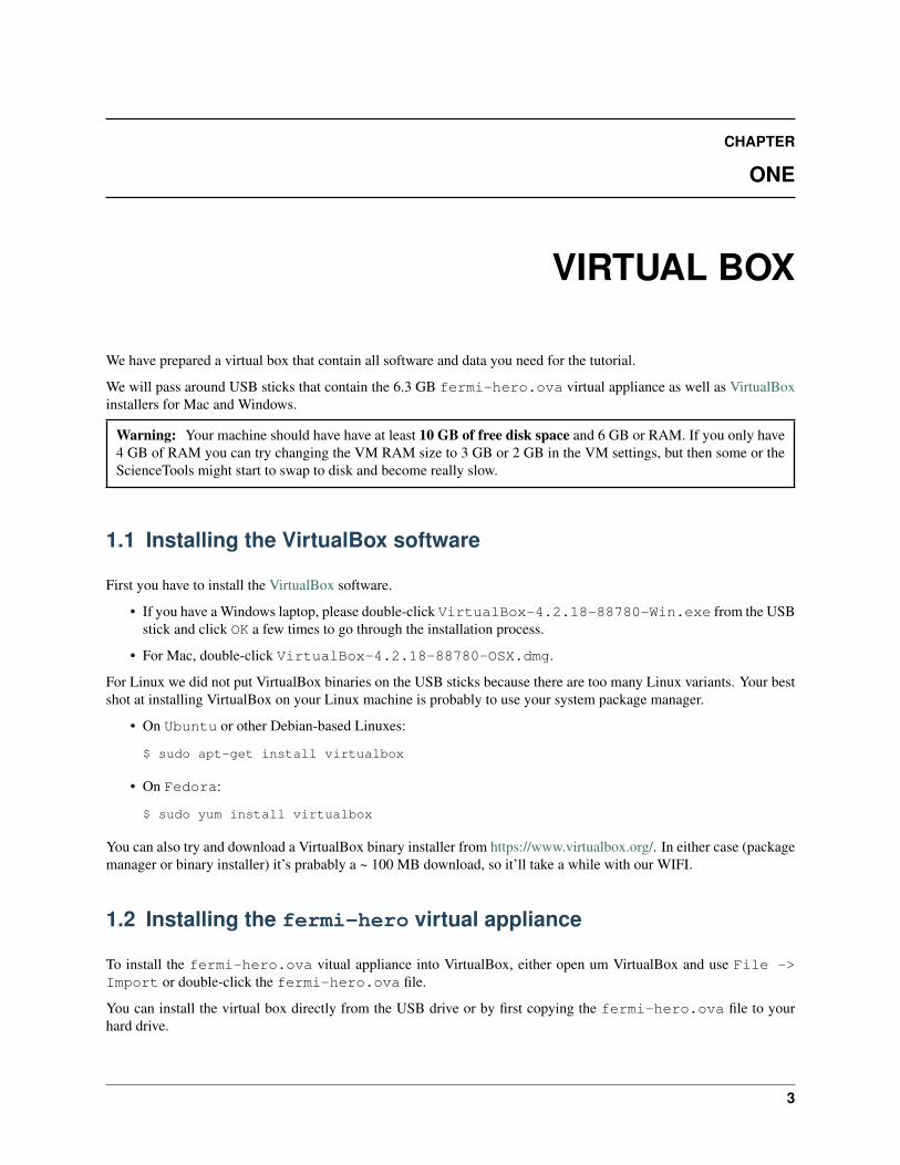
We have prepared a virtual box that contain all software and data you need for the tutorial.

We will pass around USB sticks that contain the 6.3 GB fermi-hero.ova virtual appliance as well as VirtualBoxinstallers for Mac and Windows.

Warning: Your machine should have have at least 10 GB of free disk space and 6 GB or RAM. If you only have4 GB of RAM you can try changing the VM RAM size to 3 GB or 2 GB in the VM settings, but then some or theScienceTools might start to swap to disk and become really slow.

1.1 Installing the VirtualBox software

First you have to install the VirtualBox software.

• If you have a Windows laptop, please double-click VirtualBox-4.2.18-88780-Win.exe from the USBstick and click OK a few times to go through the installation process.

• For Mac, double-click VirtualBox-4.2.18-88780-OSX.dmg.

For Linux we did not put VirtualBox binaries on the USB sticks because there are too many Linux variants. Your bestshot at installing VirtualBox on your Linux machine is probably to use your system package manager.

• On Ubuntu or other Debian-based Linuxes:

$ sudo apt-get install virtualbox

• On Fedora:

$ sudo yum install virtualbox

You can also try and download a VirtualBox binary installer from https://www.virtualbox.org/. In either case (packagemanager or binary installer) it’s prabably a ~ 100 MB download, so it’ll take a while with our WIFI.

1.2 Installing the fermi-hero virtual appliance

To install the fermi-hero.ova vitual appliance into VirtualBox, either open um VirtualBox and use File ->Import or double-click the fermi-hero.ova file.

You can install the virtual box directly from the USB drive or by first copying the fermi-hero.ova file to yourhard drive.

3

fermi-hero Documentation, Release 0.1

In any case this will create a virtual box called fermi-hero on your had disk (a folder called fermi-hero witha large fermi-hero.vdi file, a small fermi-hero.vbox file as well as some other stuff inside. You’ll neverhave to look at this folder, except if you are short on disk space check it’s size.

Note: VMWare should also be capable of importing the fermi-hero.vdi appliance, so if you prefer VMWare(non-free, but a bit nicer in some ways) over VirtualBox (free), give it a try and let us know.

1.3 Starting and using the fermi-hero virtual machine

To start the fermi-hero virtual machine (VM), start VirtualBox (the window has Oracle VM VirtualBoxManager in the title) and double-click on the fermi-hero VM.

Fedora wil boot up and present you with a login screen for the user hero.

Some information on the VM:

• Distributed as 6.3 GB file fermi-hero.ova in the Open Virtualization Format

• 20 GB disk (VM file size grows dynamically) in VDI format

• 4 GB RAM

• 64-bit Fedora Linux Version 19 (specifically Fedora-Live-Desktop-x86_64-19-1.iso)

• Do all analysis as user hero in the home directory /home/hero ... no login password set.

• If you need root access ... the password is root. E.g. you can get a root terminal by typing su and theninstall software using yum.

4 Chapter 1. Virtual Box

CHAPTER

TWO

SOFTWARE

Warning: Please do not download large files during the tutorial or the WIFI network will overload. We willdistribute the software and data you need via USB sticks.

To participate in the tutorial you should bring a Mac or Linux laptop.

This page describes how to install the software we need for the tutorial and how to check that it works properly.

If you have a Windows laptop, you can install VirtualBox and then install Linux in a virtual machine. It’s best to installa Linux distribution that is officially supported by the Fermi science tools (see here): unfortunately the Scientific Linuxdistribution is very large (over 4 GB) and Ubuntu has known problems. Therefore we recomment you try Fedora,which should be similar enough to ScientificLinux for the Scientific Linux 6 64 bit libc 2.12 binary version of theScienceTools to work.

Check: you should be able to open a terminal and do this:

$ echo "Hello world"Hello world$

2.1 Overview

You should install the following software:

• Fermi Science Tools

• FTOOLS = HEASOFT (includes fv)

• ds9

• TOPCAT

• Aladin (if you want)

• Enrico

2.2 Fermi Science Tools

The main analysis software you will use for this tutorial is the Fermi data analysis software, called the Fermi sciencetools.

5

fermi-hero Documentation, Release 0.1

The Fermi Science Support Center web pages contain a lot of information about Fermi data access and data analysis.If you have a problem you can’t solve yourself (always try finding a solution yourself with Google first), you cancontact the official NASA Fermi help desk or post in this forum.

The most important piece of advice on the Installing the Fermi Science Tools page is:

> Downloading and installing the Fermi science tools from the binary tar files below is strongly recommended. > Themany minor variations in the various Unix systems makes building the tools from source challenging.

So download the binary tar file for your machine ... this will take a while becauseit’s about 1 GB in size. As an example, for Mac the file you get will be calledScienceTools-v9r31p1-fssc-20130410-x86_64-apple-darwin12.2.0.tar.gzor maybe if it is automatically unzipped after download it will be calledScienceTools-v9r31p1-fssc-20130410-x86_64-apple-darwin12.2.0.tar.

After download you have to set up the Fermi science tools as described here.

Check: you should be able to use the Fermi science tools from the Shell command line and via Python:

$ which gtbin$ gtbin# abort with CTRL + C$ which python$ python>>> import UnbinnedAnalysis

2.2.1 libcrypto and libssl shared library problem

If gtbin complains about missing libcrypto.so.10, then you need make a link to your installed version with thename requested. To do this first use locate to find your version, then cd to that directory and create a symbolic link.Example:

$ sudo -i# locate libcrypto/PATH TO FILE/libcrypto.so.0.9.8# cd /PATH TO FILE/# ln -s libcrypto.so.0.9.8 libcrypto.so.10

You see either a file called libcrypto.so.0.9.8 or libcrypto.so.1.0.0. If locate finds a file calledlibcrypto.so.1.0.0, use that file instead of the libcrypto.0.9.8 version.

After creating the libcrypto link, try to run gtbin. Sometimes a similar error regarding libssl will take place,if it does repeat the steps above with thelibssl file to (hopefully) correct it.

2.3 FTOOLS = HEASOFT

Next install the FTOOLS — A General Package of Software to Manipulate FITS Files following the in-stallation instructions on the web. To install correctly you must run the configure script found inheasoft-6.14/[platform version]/BUILD_DIR, where [platform version] corresponds to thestring of your platform (e.g., x86_64-unknown-linux-gnu-libc2.5 for Linux64).

With the FTOOLS you install Fv: The Interactive FITS File Editor, a flexible tool to view and edit FITS files.

E.g. the ftlist command line tool is very handy to check what is in a given FITS file.

Use ds9 as an image viewer and fv to look at the content of Fermi event lists (called photon files).

Check: Open up a Fermi event list as described here with fv

6 Chapter 2. Software

fermi-hero Documentation, Release 0.1

2.4 ds9

SAOImage DS9 is one of the best viewers for astronomical 2D images and 3D cubes ... please download it from here.

Check: Download and open up the following FITS files:

• Hubble space telescope image of the Antennae Galaxies (FITS file of the 2D image)

• Fermi LAT diffuse emission model (an outdated version, used here because of the small file size) (FITS file ofthe 3D cube with log(energy) on the third axis).

If you want:

• Some Hubble space telescope optical images here.

• Some Chandra X-ray observatory X-ray images here

2.5 TOPCAT

TOPCAT <http://www.star.bris.ac.uk/~mbt/topcat/> is a Java program to view FITS tables. Follow the installationinstructions on the web.

2.6 Aladin (optional)

Aladin — A FITS image viewer (alternative to ds9) is a nice astronomical image and catalog viewer ... an alternativeto ds9.

Install it and give it a try if you want.

2.7 Enrico

Producing a spectrum (global model and flux points in energy bins) or light curve (flux points in time bins) requirescalling a lot of Fermi science tools with the right parameters in the right order.

Luckily you have Enrico to help you. Enrico is a set of Python scripts that take a single config file as input whereyou specify what kind of analysis you want to run and the most important analysis parameters, and the run all Fermiscience tools in the right order (or in parallel where possible) with the right parameters for you.

Please install Enrico as described here.

Check: To check that Enrico is installed correctly run this command:

$ enrico_setupcheck

2.8 Init file

You should create a file fermi-hero-init.sh which sets up your shell for this tutorial.

Once all software is installed all you have to do is:

$ source fermi-hero-init.sh

2.4. ds9 7

fermi-hero Documentation, Release 0.1

This is an example init file ... you’ll have to adapt the PATHs / versions to your system:

export FERMI_HERO = /Users/deil/FERMI_HERO

export HEADAS=$FERMI_HERO/heasoft-6.14/x86_64-unknown-linux-gnu-libc2.5source $HEADAS/headas-init.sh

export FERMI_DIR=$FERMI_HERO/ScienceTools-v9r31p1-fssc-20130410-x86_64-apple-darwin12.2.0/x86_64-apple-darwin12.2.0source $FERMI_DIR/fermi-init.sh

export ENRICO_DIR=$FERMI_HERO/enricosource $ENRICO_DIR/enrico-init.sh

alias topcat="java -Xms512m -Xmx4024m -jar /Applications/TOPCAT.app/Contents/Resources/Java/topcat-full.jar"alias aladin="java -Xms512m -Xmx4024m -jar /Applications/Aladin.app/Contents/Resources/Java/Aladin.jar"

# Add location of binaries to your PATH, e.g. for ds9:export PATH=$PATH:$FERMI_HERO

8 Chapter 2. Software

CHAPTER

THREE

DATA

Warning: Please do not download large files during the tutorial or the WIFI network will overload. We willdistribute the software and data you need via USB sticks.

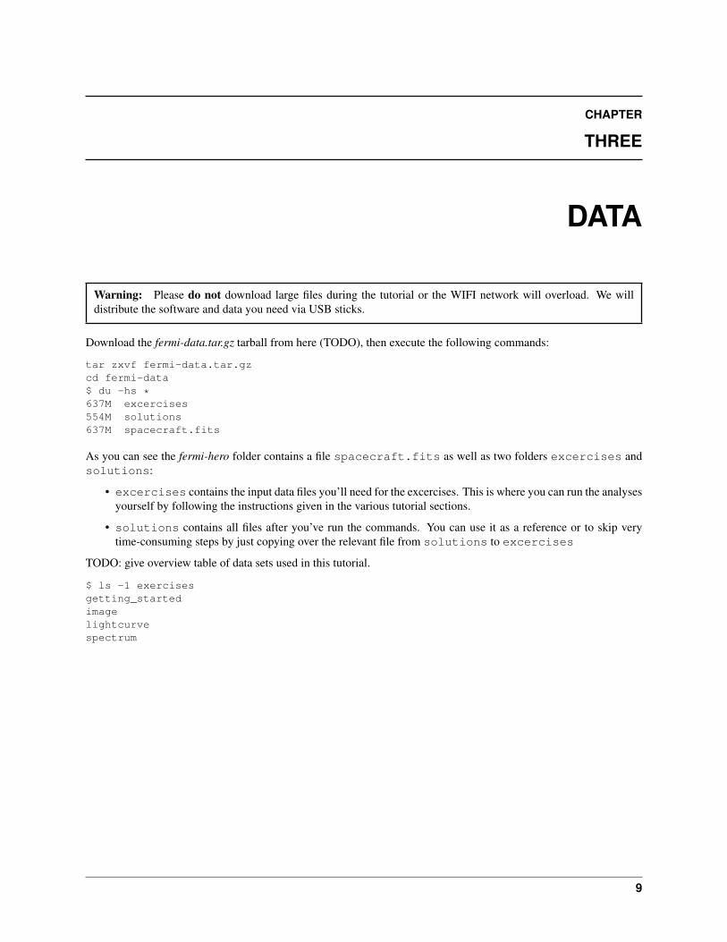
Download the fermi-data.tar.gz tarball from here (TODO), then execute the following commands:

tar zxvf fermi-data.tar.gzcd fermi-data$ du -hs *637M excercises554M solutions637M spacecraft.fits

As you can see the fermi-hero folder contains a file spacecraft.fits as well as two folders excercises andsolutions:

• excercises contains the input data files you’ll need for the excercises. This is where you can run the analysesyourself by following the instructions given in the various tutorial sections.

• solutions contains all files after you’ve run the commands. You can use it as a reference or to skip verytime-consuming steps by just copying over the relevant file from solutions to excercises

TODO: give overview table of data sets used in this tutorial.

$ ls -1 exercisesgetting_startedimagelightcurvespectrum

9

fermi-hero Documentation, Release 0.1

10 Chapter 3. Data

CHAPTER

FOUR

GETTING STARTED

To get started, you will learn how to use some tools to download, prepare and explore Fermi LAT data.

Fermi LAT data consists of event data files and spacecraft data files.

Note: Throughout this tutorial we will use the terms event and photon interchangeably, because for the event classeswe use the fraction of events that are not photons, but charged cosmic rays, is negligibly low (less than 1%).

Event file == Photon file == FT1 file

Spacecraft file == FT2 file

The spacecraft data file contains the information about the orbit position and pointing direction as well as some statusand quality information ... you can use the same spacecraft file (~700 MB for 5 years) for all your analyses as long asit covers the time range you want to analyse. That’s all you need to know about the spacecraft data file ... simply giveit’s filename to the tools that require it to do their job.

The event data file contains a table of observed and reconstructed events. where the most important event parametersare:

• (RA, DEC) (degrees). Equatorial coordinates ... called right ascension RA and declination DEC.

• (L, B) (degrees). Galactic coordinates ... called Galactic longitude L and latitude B.

• ENERGY (MeV)

• TIME (seconds). Mission elapsed time when the event was detected. (MET is the total number of seconds since00:00:00 on January 1, 2001 UTC)

In this tutorial we will have a quick look at the Fermi LAT dataset by binning the events into histograms:

• A 2-dimensional (L, B) histogram is called a counts image.

• A 1-dimensional ENERGY histogram is called a counts spectrum.

• A 1-dimensional TIME histogram is called a counts lightcurve.

In the Spectrum, Aperture Lightcurve and Galactic Center High-Energy View tutorials we will then show you how tocreate a flux spectrum, flux lightcurve and flux image, where flux = counts / exposure and exposure = (effectivearea) x (observation time) and in addition to exposure the spatial resolution, called point spread function (PSF), andenergy resolution have been taken into account.

If you are interested to at least get a basic understanding of the theory how Fermi LAT gamma-ray data analysis works,have a look at the Fermi LAT Instrument response functions and Fermi LAT Likelihood Analysis section of the FermiLAT Manual, called Cicerone. In this short Fermi-Hero tutorial we focus on how to use the tools to obtain resultsinstead of what exactly the tools do and why (methods, theory).

11

fermi-hero Documentation, Release 0.1

4.1 Prerequisites

You should have installed and quickly tested the Software and downloaded and extracted the Fermi-Hero tutorial Data.

4.2 Steps

4.2.1 First look at Fermi LAT photon files with ftlist and fv

Event files like L1309081333300B976F4377_PH00.fits are FITS files. FITS is the standard data format inastronomy for arrays (e.g. 2D images) and tables (e.g. source catalogs or event lists).

Let’s use a few different tools to explore the content of L1309081333300B976F4377_PH00.fits.

List photon file contents with ftlist

ftlist is a command-line tool to ... duh ... list the content of FITS files. A FITS file consists of header-data units(HDUs), where each HDU is an array or table. For historic reasons the first HDU (a.k.a. primary HDU) has to be anarray, so in FITS files that only contain tabular data the primary HDU will be a dummy, empty HDU.

Giving a filename and the print option H to list a 1-line summary of the HDUs to ftlist we get:

$ ftlist L1309081333300B976F4377_PH00.fits H

Name Type Dimensions---- ---- ----------

HDU 1 Primary Array Null ArrayHDU 2 EVENTS BinTable 22 cols x 1065513 rowsHDU 3 GTI BinTable 2 cols x 1790 rows

So this event file contains an EVENTS table with 1065513 events and a GTI (good time interval) table with 1790GTIs. GTIs are needed to compute exposure. Exposure is needed to compute the flux of sources.

To list the names and units of the columns in the EVENTS and GTI table use the C print option with ftlist:

$ ftlist L1309081333300B976F4377_PH00.fits CHDU 2

Col Name Format[Units](Range) Comment1 ENERGY E [MeV] (0.:10000000.)2 RA E [deg] (0.:360.)3 DEC E [deg] (-90.:90.)4 L E [deg] (0.:360.)5 B E [deg] (-90.:90.)6 THETA E [deg] (0.:180.)7 PHI E [deg] (0.:360.)8 ZENITH_ANGLE E [deg] (0.:180.)9 EARTH_AZIMUTH_ANGLE E [deg] (0.:360.)

10 TIME D [s] (0.:10000000000.)11 EVENT_ID J (0:2147483647)12 RUN_ID J (0:2147483647)13 RECON_VERSION I (0:32767)14 CALIB_VERSION 3I15 EVENT_CLASS J (0:32767)16 CONVERSION_TYPE I (0:32767)17 LIVETIME D [s] (0.:10000000000.)

12 Chapter 4. Getting Started

fermi-hero Documentation, Release 0.1

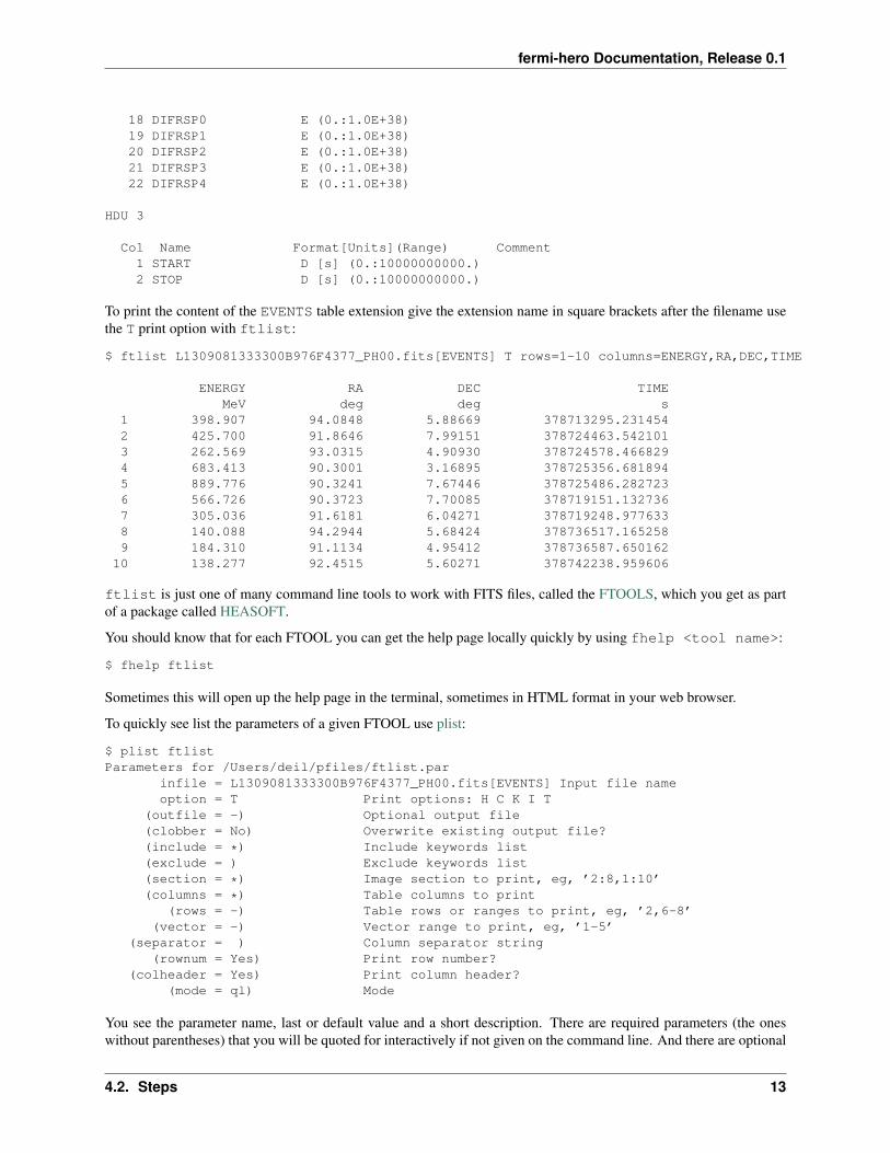
18 DIFRSP0 E (0.:1.0E+38)19 DIFRSP1 E (0.:1.0E+38)20 DIFRSP2 E (0.:1.0E+38)21 DIFRSP3 E (0.:1.0E+38)22 DIFRSP4 E (0.:1.0E+38)

HDU 3

Col Name Format[Units](Range) Comment1 START D [s] (0.:10000000000.)2 STOP D [s] (0.:10000000000.)

To print the content of the EVENTS table extension give the extension name in square brackets after the filename usethe T print option with ftlist:

$ ftlist L1309081333300B976F4377_PH00.fits[EVENTS] T rows=1-10 columns=ENERGY,RA,DEC,TIME

ENERGY RA DEC TIMEMeV deg deg s

1 398.907 94.0848 5.88669 378713295.2314542 425.700 91.8646 7.99151 378724463.5421013 262.569 93.0315 4.90930 378724578.4668294 683.413 90.3001 3.16895 378725356.6818945 889.776 90.3241 7.67446 378725486.2827236 566.726 90.3723 7.70085 378719151.1327367 305.036 91.6181 6.04271 378719248.9776338 140.088 94.2944 5.68424 378736517.1652589 184.310 91.1134 4.95412 378736587.650162

10 138.277 92.4515 5.60271 378742238.959606

ftlist is just one of many command line tools to work with FITS files, called the FTOOLS, which you get as partof a package called HEASOFT.

You should know that for each FTOOL you can get the help page locally quickly by using fhelp <tool name>:

$ fhelp ftlist

Sometimes this will open up the help page in the terminal, sometimes in HTML format in your web browser.

To quickly see list the parameters of a given FTOOL use plist:

$ plist ftlistParameters for /Users/deil/pfiles/ftlist.par

infile = L1309081333300B976F4377_PH00.fits[EVENTS] Input file nameoption = T Print options: H C K I T

(outfile = -) Optional output file(clobber = No) Overwrite existing output file?(include = *) Include keywords list(exclude = ) Exclude keywords list(section = *) Image section to print, eg, ’2:8,1:10’(columns = *) Table columns to print

(rows = -) Table rows or ranges to print, eg, ’2,6-8’(vector = -) Vector range to print, eg, ’1-5’

(separator = ) Column separator string(rownum = Yes) Print row number?

(colheader = Yes) Print column header?(mode = ql) Mode

You see the parameter name, last or default value and a short description. There are required parameters (the oneswithout parentheses) that you will be quoted for interactively if not given on the command line. And there are optional

4.2. Steps 13

fermi-hero Documentation, Release 0.1

parameters (the ones in parentheses) that you have to give on the command line if you want to choose a different valuethan the default.

Plot a photon zenith angle histogram with fv

Next let’s use Fv: The Interactive FITS File Editor. ftlist was a command line tool ... fv is a GUI (graphical userinterface) tool.

Open fv and the event file like this:

$ fv L1309081333300B976F4377_PH00.fits

or if you prefer to run fv in the background like this:

$ fv L1309081333300B976F4377_PH00.fits &

The advantage of running tools in the background is that you can execute other commands without having to wait forthe tool to finish or having to open an extra terminal window.

fv is very powerful, but because it’s so ugly that it probably makes your eyes hurt we’ll only use it to do one thing:plot a the distribution of the ZENITH_ANGLE of the EVENTS.

• Click the Histogram button for the EVENTS HDU.

• In the dialog window called Histogram select ZENITH_ANGLE as column name for X. In this case the defaultbinning options are reasonable ... click Make/Close.

• Done. A window called POW shows the zenith angle histogram.

• In the fv menu click Quit, then No to All in the exit dialog window to confirm that you don’t want topermanently save the temp histogram file.

14 Chapter 4. Getting Started

fermi-hero Documentation, Release 0.1

The zenith angle histogram shows a broad peak in the range 0 deg to 100 deg, and a narrow peak around 113 deg.

We’ll explain the origin and relevance of this distribution in the next section Prepare Fermi LAT data with gtselect andgtmktime.

4.2.2 Get Fermi LAT data

Spacecraft file

The spacecraft file doesn’t depend on the sky region or energy range you are interested in ... it is valid for the wholesky and all energies.

The only thing you have to watch out for is that your spacecraft file covers the time range you want to analyse. Toobtain a spacecraft data file that covers the whole length of the Fermi mission (updated daily with new data) use thiscommand

wget -O spacecraft.fits ftp://legacy.gsfc.nasa.gov/FTP/fermi/data/lat/mission/spacecraft/lat_spacecraft_merged.fits

Photon files

Usually you will do this via the FSSC data query web interface as described in the Extract LAT Data analysis thread.

TODO: give screenshots and short description.

4.2. Steps 15

fermi-hero Documentation, Release 0.1

Tip: If you are a Fermi LAT power user (e.g. run analyses on several regions or update your analyses every once ina while) or if there are several Fermi LAT data analysts at your institute you should consider downloading the weeklyphoton and spacecraft files as described here:

wget -m -P . -nH --cut-dirs=4 -np -e robots=off \ftp://legacy.gsfc.nasa.gov/fermi/data/lat/weekly/photon/wget -m -P . -nH --cut-dirs=4 -np -e robots=off \ftp://legacy.gsfc.nasa.gov/fermi/data/lat/weekly/spacecraft/

Note that the weekly photon files currently (2013, covering five years of Fermi observations) are about 30 GB (giga-bytes) in size, so make sure you have the disk space and internet connection bandwidth.

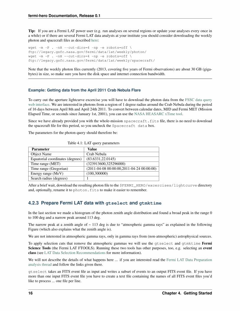
Example: Getting data from the April 2011 Crab Nebula Flare

To carry out the aperture lightcurve excercise you will have to download the photon data from the FSSC data queryweb interface. We are interested in photons from a region of 1 degree radius around the Crab Nebula during the periodof 16 days between April 8th and April 24th 2011. To convert between calendar dates, MJD and Fermi MET (MissionElapsed Time, or seconds since January 1st, 2001), you can use the NASA HEASARC xTime tool.

Since we have already provided you with the whole-mission spacecraft.fits file, there is no need to downloadthe spacecraft file for this period, so you uncheck the Spacecraft data box.

The parameters for the photon query should therefore be:

Table 4.1: LAT query parameters

Parameter ValueObject Name Crab NebulaEquatorial coordinates (degrees) (83.6331,22.0145)Time range (MET) (323913600,325296000)Time range (Gregorian) (2011-04-08 00:00:00,2011-04-24 00:00:00)Energy range (MeV) (100,300000)Search radius (degrees) 1

After a brief wait, download the resulting photon file to the $FERMI_HERO/excercises/lightcurve directoryand, optionally, rename it to photon.fits to make it easier to remember.

4.2.3 Prepare Fermi LAT data with gtselect and gtmktime

In the last section we made a histogram of the photon zenith angle distribution and found a broad peak in the range 0to 100 deg and a narrow peak around 113 deg.

The narrow peak at a zenith angle of ~ 113 deg is due to “atmospheric gamma rays” as explained in the followingFigure (which also explains what the zenith angle is).

We are not interested in atmospheric gamma rays, only in gamma rays from (non-atmospheric) astrophysical sources.

To apply selection cuts that remove the atmospheric gammas we will use the gtselect and gtmktime FermiScience Tools (the Fermi LAT FTOOLS). Running these two tools has other purposes, too, e.g. selecting an eventclass (see LAT Data Selection Recommendations for more information).

We will not describe the details of what happens here ... if you are interested read the Fermi LAT Data Preparationanalysis thread and follow the links given there.

gtselect takes an FITS event file as input and writes a subset of events to an output FITS event file. If you havemore than one input FITS event file you have to create a text file containing the names of all FITS event files you’dlike to process ... one file per line.

16 Chapter 4. Getting Started

fermi-hero Documentation, Release 0.1

Figure 4.1: Schematic of Limb gamma-ray production by cosmic ray interactions in the Earth’s atmosphere, showingthe definitions of the zenith angle (θz), the spacecraft rocking angle (θr) and the incidence angle (θ). Reference:http://adsabs.harvard.edu/abs/2013arXiv1305.5597F

Use the command line ls utility to create the text file and the cat utility to print it’s contents to the terminal to checkthat it worked:

$ ls -1 *_PH??.fits > events.txt$ cat events.txtL1309081333300B976F4377_PH00.fitsL1309081333300B976F4377_PH01.fits

Now run gtselect and select event class 2, corresponding to P7SOURCE_V6, as well as a maximum zenith angle of100 deg as recommended here:

$ gtselect evclass=2Input FT1 file[] @events.txtOutput FT1 file[] gtselect.fitsRA for new search center (degrees) (0:360) [] INDEFDec for new search center (degrees) (-90:90) [] INDEFradius of new search region (degrees) (0:180) [] INDEFstart time (MET in s) (0:) [] INDEFend time (MET in s) (0:) [] INDEFlower energy limit (MeV) (0:) [] 100upper energy limit (MeV) (0:) [] 1000000maximum zenith angle value (degrees) (0:180) [] 100Done.

Note that we had to specify the evclass parameter on the command line, because it’s a hidden FTOOL parameter:

$ plist gtselectParameters for /Users/deil/pfiles/gtselect.par

infile = @events.txt Input FT1 fileoutfile = gtselect.fits Output FT1 file

ra = INDEF RA for new search center (degrees)

4.2. Steps 17

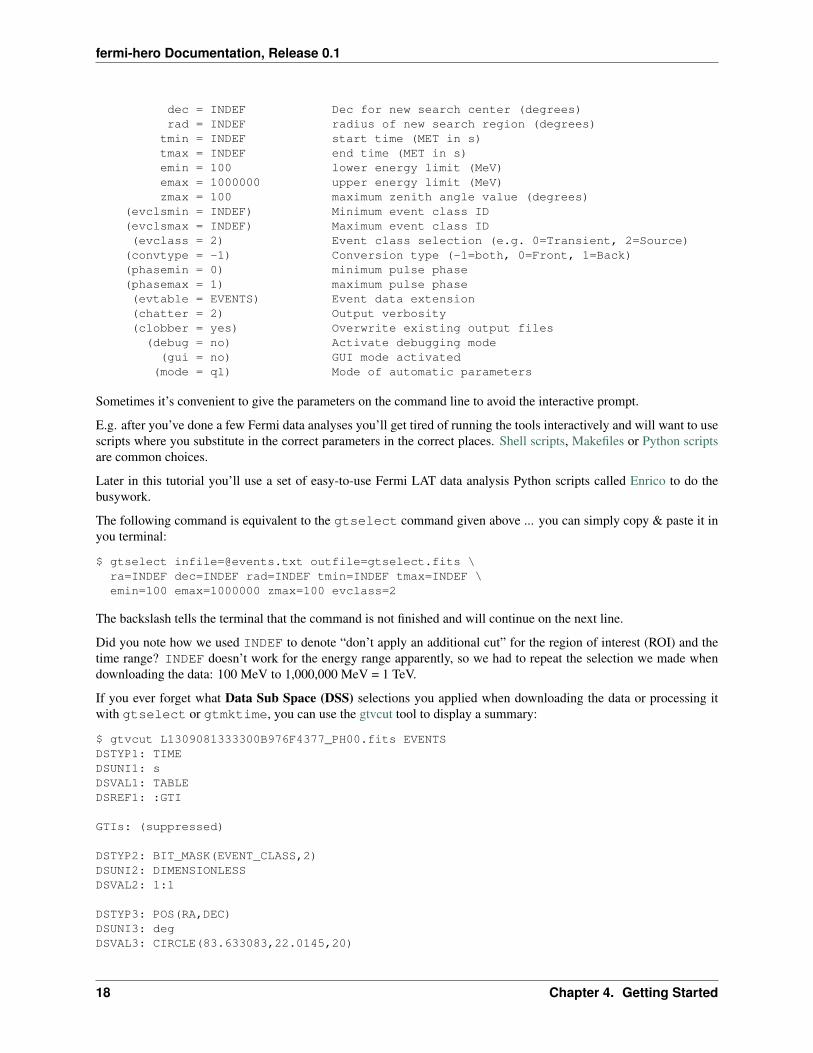
fermi-hero Documentation, Release 0.1

dec = INDEF Dec for new search center (degrees)rad = INDEF radius of new search region (degrees)

tmin = INDEF start time (MET in s)tmax = INDEF end time (MET in s)emin = 100 lower energy limit (MeV)emax = 1000000 upper energy limit (MeV)zmax = 100 maximum zenith angle value (degrees)

(evclsmin = INDEF) Minimum event class ID(evclsmax = INDEF) Maximum event class ID(evclass = 2) Event class selection (e.g. 0=Transient, 2=Source)

(convtype = -1) Conversion type (-1=both, 0=Front, 1=Back)(phasemin = 0) minimum pulse phase(phasemax = 1) maximum pulse phase(evtable = EVENTS) Event data extension(chatter = 2) Output verbosity(clobber = yes) Overwrite existing output files

(debug = no) Activate debugging mode(gui = no) GUI mode activated(mode = ql) Mode of automatic parameters

Sometimes it’s convenient to give the parameters on the command line to avoid the interactive prompt.

E.g. after you’ve done a few Fermi data analyses you’ll get tired of running the tools interactively and will want to usescripts where you substitute in the correct parameters in the correct places. Shell scripts, Makefiles or Python scriptsare common choices.

Later in this tutorial you’ll use a set of easy-to-use Fermi LAT data analysis Python scripts called Enrico to do thebusywork.

The following command is equivalent to the gtselect command given above ... you can simply copy & paste it inyou terminal:

$ gtselect infile=@events.txt outfile=gtselect.fits \ra=INDEF dec=INDEF rad=INDEF tmin=INDEF tmax=INDEF \emin=100 emax=1000000 zmax=100 evclass=2

The backslash tells the terminal that the command is not finished and will continue on the next line.

Did you note how we used INDEF to denote “don’t apply an additional cut” for the region of interest (ROI) and thetime range? INDEF doesn’t work for the energy range apparently, so we had to repeat the selection we made whendownloading the data: 100 MeV to 1,000,000 MeV = 1 TeV.

If you ever forget what Data Sub Space (DSS) selections you applied when downloading the data or processing itwith gtselect or gtmktime, you can use the gtvcut tool to display a summary:

$ gtvcut L1309081333300B976F4377_PH00.fits EVENTSDSTYP1: TIMEDSUNI1: sDSVAL1: TABLEDSREF1: :GTI

GTIs: (suppressed)

DSTYP2: BIT_MASK(EVENT_CLASS,2)DSUNI2: DIMENSIONLESSDSVAL2: 1:1

DSTYP3: POS(RA,DEC)DSUNI3: degDSVAL3: CIRCLE(83.633083,22.0145,20)

18 Chapter 4. Getting Started

fermi-hero Documentation, Release 0.1

DSTYP4: TIMEDSUNI4: sDSVAL4: 378691200:394329600

DSTYP5: ENERGYDSUNI5: MeVDSVAL5: 100:1000000

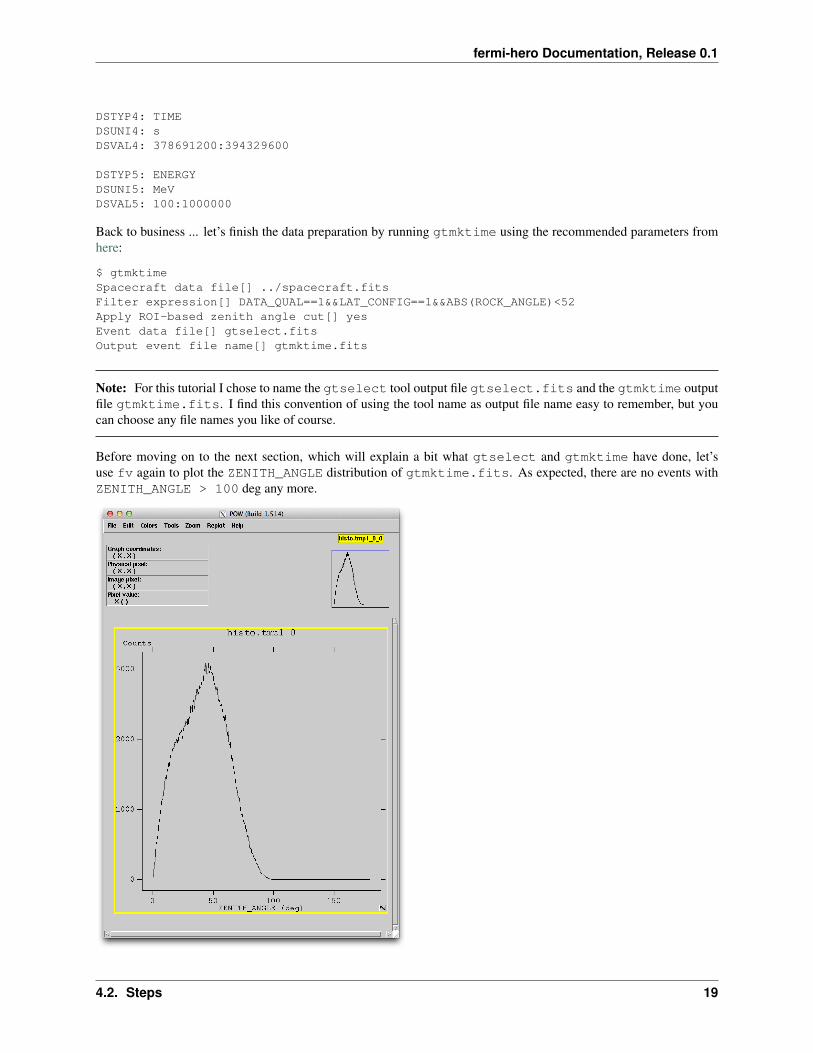
Back to business ... let’s finish the data preparation by running gtmktime using the recommended parameters fromhere:

$ gtmktimeSpacecraft data file[] ../spacecraft.fitsFilter expression[] DATA_QUAL==1&&LAT_CONFIG==1&&ABS(ROCK_ANGLE)<52Apply ROI-based zenith angle cut[] yesEvent data file[] gtselect.fitsOutput event file name[] gtmktime.fits

Note: For this tutorial I chose to name the gtselect tool output file gtselect.fits and the gtmktime outputfile gtmktime.fits. I find this convention of using the tool name as output file name easy to remember, but youcan choose any file names you like of course.

Before moving on to the next section, which will explain a bit what gtselect and gtmktime have done, let’suse fv again to plot the ZENITH_ANGLE distribution of gtmktime.fits. As expected, there are no events withZENITH_ANGLE > 100 deg any more.

4.2. Steps 19

fermi-hero Documentation, Release 0.1

4.2.4 Compute data summaries with Python

In this section we will use the Python programming language interactive console and the PyFITS package and numpy(all come with the Fermi ScienceTools) to compute data summaries of the various event files.

To start Python, simply type python on the command line. This will show the Python prompt >>> where you canexecute commands. To exit Python type CTRL + D:

$ pythonPython 2.7.2 (default, Apr 12 2013, 00:51:51)[GCC 4.2.1 (Based on Apple Inc. build 5658) (LLVM build 2336.11.00)] on darwinType "help", "copyright", "credits" or "license" for more information.>>> 3 + 25>>> ^D$

To check that you are actually using the Python in the Fermi ScienceTools:

$ which python/Users/deil/software/fermi/ScienceTools-v9r31p1-fssc-20130410-x86_64-apple-darwin12.2.0/x86_64-apple-darwin12.2.0/bin/python

Remember that we had two photon files from the Fermi LAT data server and then ran gtselect to producegtselect.fits and gtmktime to produce gtmktime.fits:

$ ftlist L1309081333300B976F4377_PH00.fits H

Name Type Dimensions---- ---- ----------

HDU 1 Primary Array Null ArrayHDU 2 EVENTS BinTable 22 cols x 1065513 rowsHDU 3 GTI BinTable 2 cols x 1790 rows

$ ftlist L1309081333300B976F4377_PH01.fits H

Name Type Dimensions---- ---- ----------

HDU 1 Primary Array Null ArrayHDU 2 EVENTS BinTable 22 cols x 377253 rowsHDU 3 GTI BinTable 2 cols x 1022 rows

$ ftlist gtselect.fits H

Name Type Dimensions---- ---- ----------

HDU 1 Primary Array Null ArrayHDU 2 EVENTS BinTable 22 cols x 365387 rowsHDU 3 GTI BinTable 2 cols x 2812 rows

$ ftlist gtmktime.fits H

Name Type Dimensions---- ---- ----------

HDU 1 Primary Array Null ArrayHDU 2 EVENTS BinTable 22 cols x 312629 rowsHDU 3 GTI BinTable 2 cols x 3419 rows

Just to get used to Python and PyFITS, let’s explore a bit what gtselect and gtmktime have done to the EVENTSand GTIs:

20 Chapter 4. Getting Started

fermi-hero Documentation, Release 0.1

$ pythonPython 2.7.2 (default, Apr 12 2013, 00:51:51)[GCC 4.2.1 (Based on Apple Inc. build 5658) (LLVM build 2336.11.00)] on darwinType "help", "copyright", "credits" or "license" for more information.>>> 1790 + 10222812>>> import pyfits>>> ph00 = pyfits.open(’L1309081333300B976F4377_PH00.fits’)>>> ph01 = pyfits.open(’L1309081333300B976F4377_PH01.fits’)>>> gtselect = pyfits.open(’gtselect.fits’)>>> gtmktime = pyfits.open(’gtmktime.fits’)>>> ph00.info()Filename: L1309081333300B976F4377_PH00.fitsNo. Name Type Cards Dimensions Format0 PRIMARY PrimaryHDU 31 () uint81 EVENTS BinTableHDU 169 1065513R x 22C [E, E, E, E, E, E, E, E, E, D, J, J, I, 3I, J, I, D, E, E, E, E, E]2 GTI BinTableHDU 46 1790R x 2C [D, D]

TODO: finish this with some numpy calculations

4.2.5 Explore Fermi LAT photon data with TOPCAT

Now that we have a prepared the event list to only contain astrophysical photons let’s have a look at the (RA, DEC),(L, B) as well as ENERGY and TIME distributions of the events.

TOPCAT

TOPCAT is the “Tool for OPerations on Catalogues And Tables”. Open the preprocessed event list with will open themain window with TOPCAT in the title and by default select the GTI HDU (called location gtmktime.fits-2 andname GTI-1):

$ topcat gtmktime.fits

• In the table list on the left side of the main window, select the first HDU. You should see Name: EVENTS-1in the Current Table Properties section.

• Open the Row Statistics window by clicking the button with the upper-case greek sigma.

4.2. Steps 21

fermi-hero Documentation, Release 0.1

Using TOPCAT is quite easy and it has a good manual, so we will not give detailed instructions how to make thefollowing plots ... with some trial and error you should be able to figure it out yourself.

Spatial distribution

TODO: explain sources and diffuse emission and PSF Point to Make an image with gtbin and view it with ds9 tutorialand Galactic Center High-Energy View tutorial.

Energy distribution

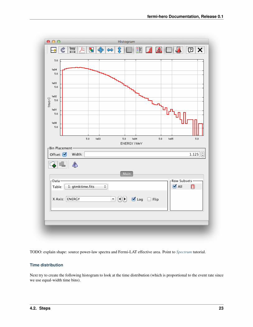
Try to create the following histogram to look at the energy distribution:

22 Chapter 4. Getting Started

fermi-hero Documentation, Release 0.1

TODO: explain shape: source power-law spectra and Fermi-LAT effective area. Point to Spectrum tutorial.

Time distribution

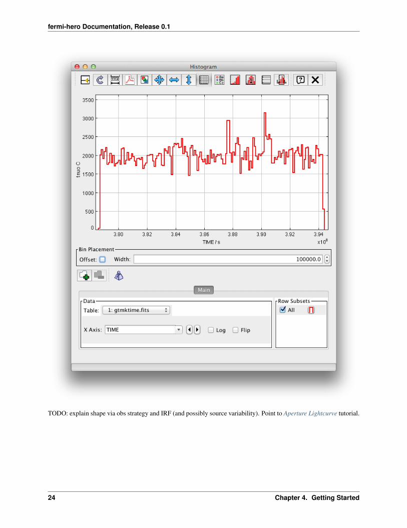
Next try to create the following histogram to look at the time distribution (which is proportional to the event rate sincewe use equal-width time bins).

4.2. Steps 23

fermi-hero Documentation, Release 0.1

TODO: explain shape via obs strategy and IRF (and possibly source variability). Point to Aperture Lightcurve tutorial.

24 Chapter 4. Getting Started

fermi-hero Documentation, Release 0.1

4.2.6 Make an image with gtbin and view it with ds9

gtbin

gtbin

ds9

ds9

4.2.7 Summary

In this “Getting Started” tutorial you have learned how to get, preprocess and explore Fermi LAT photon data filesusing many different tools:

• Command line tools: ftlist, fhelp, plist

• GUI tools: fv, TOPCAT and ds9

• (Command line) Fermi Science Tools: gtselect, gtmktime, gtvcut and gtbin

TODO: finish summary and point to next tutorial.

4.3 Additional reference

For more details, see the following official Fermi LAT analysis threads:

• Extract LAT Data

• Data Preparation

• Explore LAT Data

• Explore LAT Data (for Burst)

4.3. Additional reference 25

fermi-hero Documentation, Release 0.1

26 Chapter 4. Getting Started

CHAPTER

FIVE

SPECTRUM

In this tutorial we will perform a full likelihood analysis of the AGN PG1553+113. We will use the same datasetalready used in the official Fermi/LAT collaboration likelihood tutorial as well as in the enrico tutorial, so that youcan check your results and have additional information by consulting the two other webpages. The results from theanalysis of this dataset were published in Abdo, A. A. et al. 2010, ApJ, 708, 1310.

5.1 A note on directory structure

In order to avoid confusions, it is always best to provide absolute paths for all the files in the analysis. In this tutorialwe will assume that you have extracted the fermi-hero.tar.gz data tarball to the home directory of your user(here, as an example, we use the username hero), so that the directory structure looks like this:

$ cd /home/hero/fermi-hero$ lsexcercises solutions spacecraft.fits$ ls excercises/spectrum/L120405112547B0489E7F68_PH00.fits

To start the tutorial, change directory to /home/hero/fermi-hero/excercises/spectrum.

5.2 Make a config file

enrico uses configuration files to run analysis (for a full description see the enrico documentation on the configura-tion files).

You can use the enrico_config tool to quickly make a config file called pg1553.conf. It will ask you for the requiredoptions and copy the rest from a default config file enrico/data/config/default.conf :

$ enrico_config pg1553.confPlease provide the following required options [default] :Output directory [~/fermi-hero/excercises/spectrum] :Target Name : PG1553+113Right Ascension: 238.92935Declination: 11.190102Options are : PowerLaw, PowerLaw2, LogParabola, PLExpCutoffSpectral Model [PowerLaw] : PowerLaw2ROI Size [15] : 15FT2 file [] : ~/fermi-hero/spacecraft.fitsFT1 list of files [] : ~/fermi-hero/excercises/spectrum/L120405112547B0489E7F68_PH00.fitstag [LAT_Analysis] : spectrum

27

fermi-hero Documentation, Release 0.1

Start time [239557418] : 239557417End time [334165418] : 256970880Emin [100] : 200Emax [300000] :

Note :

• Always give the full path for the files

• We used the PowerLaw2 model as in the Fermi tutorial.

• Time is give in MET

• Energy is given in MeV

• ROI size is given in degrees

Now you can edit this config file by hand to make further adjustments.

5.3 Generate a source model xml file

The Fermi Science Tools base their likelihood analysis on a source model written in xml format. Often, this model iscomplicated to generate. You can run enrico_xml to make such model of the sky and store it into a xml file whichwill be used for the analysis. The options for this step are provided in the config file. For the enrico_xml tool, therelevant options are in the [space] and [target] sections. The out file is given by [file]/xml.

This tool automatically adds the following sources to the xml source model file:

• your target source.

• The galactic (GalDiffModel) and isotropic (IsoDiffModel) diffuse components that are the dominant backgroundsources in most LAT analysis.

• All the LAT sources from the two-year catalog (2FGL) that are inside the ROI. The spectral parameters of thesources within 3 degrees of our source are left free so they can be fit simultaneously with our source, whereasthose further away are fixed to their catalog values.

$ enrico_xml pg1553.confuse the default location of the cataloguse the default catalogUse the catalog : /CATALOG_PATH/gll_psc_v08.fitAdd 24 source(s) in the ROI of 15.0 degrees3 source(s) have free parameters inside 3.0 degrees0 source(s) is (are) extendedwrite the Xml file in /home/hero/fermi-hero/excercises/spectrum/PG1553+113_PowerLaw2_model.xml

You can explore the PG1553+113_PowerLaw2_model.xml output file with a text editor, where you will finda source xml environment for each of the sources. Additionally, the Science Tools provide the modeleditorcommand, which allows you to modify the model from a GUI.

Tip: You can find more information about the different spectral models available and their parameters at the sourcemodel definitions for gtlike and a few examples of model definitions in XML format webpages.

28 Chapter 5. Spectrum

fermi-hero Documentation, Release 0.1

5.4 Run global fit

The gtlike tool finds the best-fit parameters by minimizing a likelihood function. Before running gtlike, the usermust generate some intermediary files by using different tools. With enrico, all those steps are merged in one tool.enrico_sed will execute the following steps for you with the options you have selected in pg1553.conf:

1. gtselect: Perform event selection.

2. gtmktime: Perform time selection based on spacecraft file.

3. gtbin: Compute a counts cube map from the selected data. A counts cube map is a collection of counts mapsfor different energies.

4. gtltcube: Perform the calculation of the livetime cube. This is the most computationally intensive step, taking.

5. gtexpcube2: Use the previously generated livetime cube and apply it to your ROI to obtain an exposure cube.

6. gtsrcmaps: Create model counts maps for each of the sources in the source model catalog. This is used to speedup the likelihood calculation of gtlike.

From all the preliminary fits files generated in the previous steps, enrico is ready to run the likelihood minimisationroutine that will result in the best-fit parameters for our source of interest with the tool gtlike.

To run the global fit just call:

$ enrico_sed pg1553.conf

Warning: Computationally intensive! enrico_sed takes a long time to execute and requires significantamounts of RAM memory. As an example, in my 2011 i5 laptop the gtltcube step took 20 minutes and thegtsrcmaps took 10 minutes to run.

The command line output of the likelihood fitting should be similar to the following:

# ************************************************************# *** SUMMARY: ***# ************************************************************Source = PG1553RA = 238.929 degreesDec = 11.1901 degreesStart = 239557417.0 MET (s)Stop = 256970880.0 MET (s)ROI = 15.0 degreesE min = 100.0 MeVE max = 300000.0 MeVIRFs = P7SOURCE_V6

# ************************************************************# *** 1 gtlike --- Run likelihood analysis# ************************************************************

# ************************************************************# *** 2 Remove all the weak (TS<1) sources# ************************************************************delete source : 2FGL J1506.6+0806 with TS = 0.767925309599delete source : 2FGL J1602.4+2308 with TS = -1.51036832301delete source : 2FGL J1625.2-0020 with TS = -0.595845252567

# ************************************************************# *** 3 Re-optimize --- False# ************************************************************

5.4. Run global fit 29

fermi-hero Documentation, Release 0.1

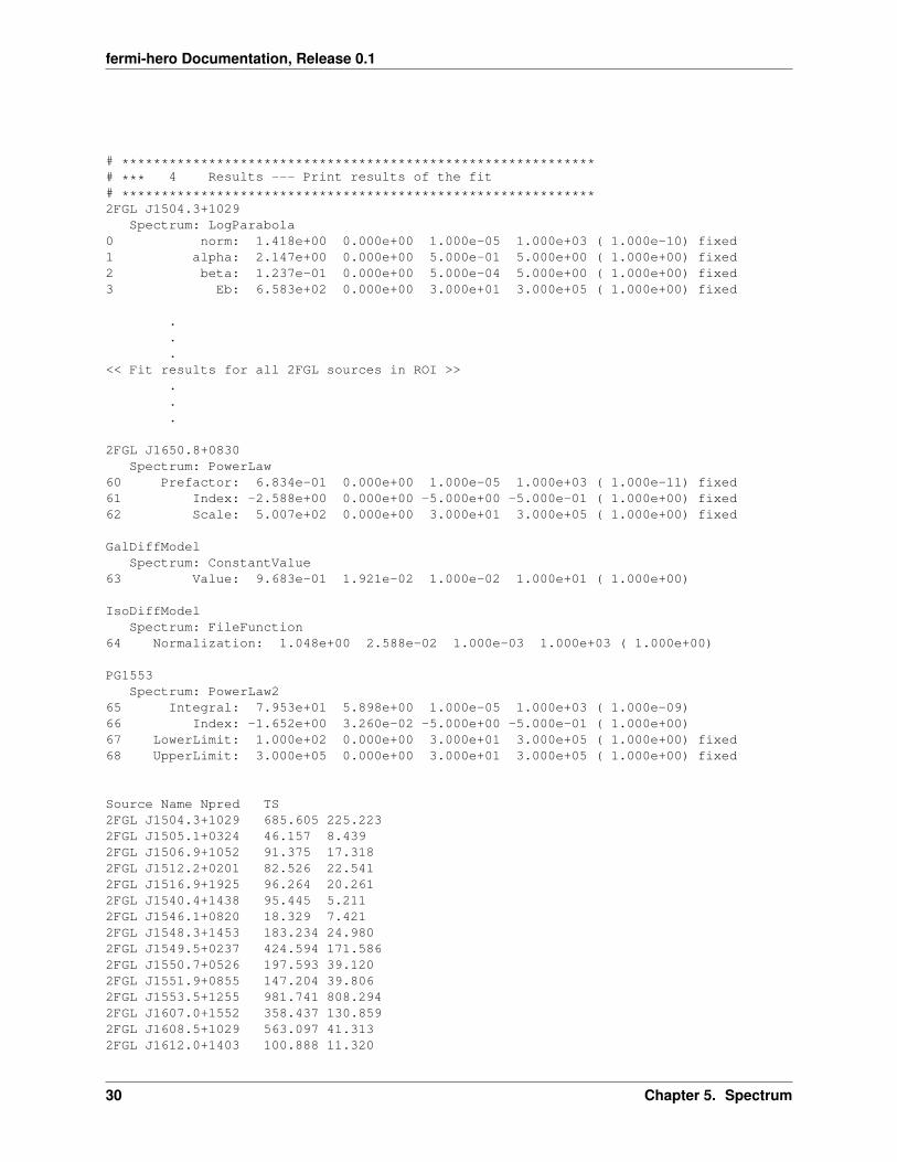
# ************************************************************# *** 4 Results --- Print results of the fit# ************************************************************2FGL J1504.3+1029

Spectrum: LogParabola0 norm: 1.418e+00 0.000e+00 1.000e-05 1.000e+03 ( 1.000e-10) fixed1 alpha: 2.147e+00 0.000e+00 5.000e-01 5.000e+00 ( 1.000e+00) fixed2 beta: 1.237e-01 0.000e+00 5.000e-04 5.000e+00 ( 1.000e+00) fixed3 Eb: 6.583e+02 0.000e+00 3.000e+01 3.000e+05 ( 1.000e+00) fixed

.

.

.<< Fit results for all 2FGL sources in ROI >>

.

.

.

2FGL J1650.8+0830Spectrum: PowerLaw

60 Prefactor: 6.834e-01 0.000e+00 1.000e-05 1.000e+03 ( 1.000e-11) fixed61 Index: -2.588e+00 0.000e+00 -5.000e+00 -5.000e-01 ( 1.000e+00) fixed62 Scale: 5.007e+02 0.000e+00 3.000e+01 3.000e+05 ( 1.000e+00) fixed

GalDiffModelSpectrum: ConstantValue

63 Value: 9.683e-01 1.921e-02 1.000e-02 1.000e+01 ( 1.000e+00)

IsoDiffModelSpectrum: FileFunction

64 Normalization: 1.048e+00 2.588e-02 1.000e-03 1.000e+03 ( 1.000e+00)

PG1553Spectrum: PowerLaw2

65 Integral: 7.953e+01 5.898e+00 1.000e-05 1.000e+03 ( 1.000e-09)66 Index: -1.652e+00 3.260e-02 -5.000e+00 -5.000e-01 ( 1.000e+00)67 LowerLimit: 1.000e+02 0.000e+00 3.000e+01 3.000e+05 ( 1.000e+00) fixed68 UpperLimit: 3.000e+05 0.000e+00 3.000e+01 3.000e+05 ( 1.000e+00) fixed

Source Name Npred TS2FGL J1504.3+1029 685.605 225.2232FGL J1505.1+0324 46.157 8.4392FGL J1506.9+1052 91.375 17.3182FGL J1512.2+0201 82.526 22.5412FGL J1516.9+1925 96.264 20.2612FGL J1540.4+1438 95.445 5.2112FGL J1546.1+0820 18.329 7.4212FGL J1548.3+1453 183.234 24.9802FGL J1549.5+0237 424.594 171.5862FGL J1550.7+0526 197.593 39.1202FGL J1551.9+0855 147.204 39.8062FGL J1553.5+1255 981.741 808.2942FGL J1607.0+1552 358.437 130.8592FGL J1608.5+1029 563.097 41.3132FGL J1612.0+1403 100.888 11.320

30 Chapter 5. Spectrum

fermi-hero Documentation, Release 0.1

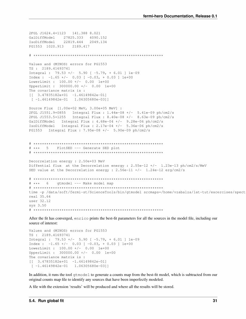
2FGL J1624.4+1123 141.388 8.021GalDiffModel 27825.333 4090.152IsoDiffModel 22819.444 2049.134PG1553 1020.913 2189.417

# ************************************************************

Values and (MINOS) errors for PG1553TS : 2189.41693741Integral : 79.53 +/- 5.90 [ -5.79, + 6.01 ] 1e-09Index : -1.65 +/- 0.03 [ -0.03, + 0.03 ] 1e+00LowerLimit : 100.00 +/- 0.00 1e+00UpperLimit : 300000.00 +/- 0.00 1e+00The covariance matrix is :[[ 3.47835182e+01 -1.46149842e-01][ -1.46149842e-01 1.06305680e-03]]

Source Flux [1.00e+02 MeV, 3.00e+05 MeV] :2FGL J1551.9+0855 Integral Flux : 1.44e-08 +/- 5.41e-09 ph/cm2/s2FGL J1553.5+1255 Integral Flux : 8.40e-08 +/- 8.63e-09 ph/cm2/sGalDiffModel Integral Flux : 4.68e-04 +/- 9.28e-06 ph/cm2/sIsoDiffModel Integral Flux : 2.17e-04 +/- 5.36e-06 ph/cm2/sPG1553 Integral Flux : 7.95e-08 +/- 5.90e-09 ph/cm2/s

# ************************************************************# *** 5 PlotSED --- Generate SED plot# ************************************************************

Decorrelation energy : 2.50e+03 MeVDiffential flux at the Decorrelation energy : 2.55e-12 +/- 1.23e-13 ph/cm2/s/MeVSED value at the Decorrelation energy : 2.56e-11 +/- 1.24e-12 erg/cm2/s

# ************************************************************# *** 6 gtmodel --- Make model map# ************************************************************time -p /data/soft/fermi-st/ScienceTools/bin/gtmodel srcmaps=/home/vzabalza/lat-tut/excercises/spectrum/PG1553_LAT_srcMap.fits srcmdl=/home/vzabalza/lat-tut/excercises/spectrum/PG1553_PowerLaw2_LAT_out.xml outfile=/home/vzabalza/lat-tut/excercises/spectrum/PG1553_LAT_ModelMap.fits irfs="P7SOURCE_V6" expcube=/home/vzabalza/lat-tut/excercises/spectrum/PG1553_LAT_ltCube.fits bexpmap=/home/vzabalza/lat-tut/excercises/spectrum/PG1553_LAT_BinnedMap.fits convol=yes resample=yes rfactor=2 outtype="CMAP" chatter=2 clobber=yes debug=no gui=no mode="ql"real 35.64user 32.12sys 3.50# ************************************************************

After the fit has converged, enrico prints the best-fit parameters for all the sources in the model file, including oursource of interest:

Values and (MINOS) errors for PG1553TS : 2189.41693741Integral : 79.53 +/- 5.90 [ -5.79, + 6.01 ] 1e-09Index : -1.65 +/- 0.03 [ -0.03, + 0.03 ] 1e+00LowerLimit : 100.00 +/- 0.00 1e+00UpperLimit : 300000.00 +/- 0.00 1e+00The covariance matrix is :[[ 3.47835182e+01 -1.46149842e-01][ -1.46149842e-01 1.06305680e-03]]

In addition, it runs the tool gtmodel to generate a counts map from the best-fit model, which is subtracted from ouroriginal counts map file to identify any sources that have been imperfectly modeled.

A file with the extension ‘results’ will be produced and where all the results will be stored.

5.4. Run global fit 31

fermi-hero Documentation, Release 0.1

Figure 5.1: Observed (left, PG1553_LAT_CountMap.fits) and model (right,PG1553_LAT_ModelMap.fits) counts maps.

Figure 5.2: Residual counts map (PG1553_Residual_Model_cmap.fits) resulting of the substraction of themodel map to the observed map. The uniform noise-like appearance and a low peak value of about 3% of the abovemaps indicate that the model accounts for all the observed emission.

32 Chapter 5. Spectrum

fermi-hero Documentation, Release 0.1

Note: If you want to refit the data because e.g. you changed the xml model, you are not force to regeneratethe fits file. Only the gtlike tool should be executed again. You can do this with enrico by changing the option[spectrum]/FitsGeneration from yes to no, and enrico will bypass all the preliminary calculations and per-form only the fit.

You can use enrico_testmodel to compute the log(likelihood) of the models PowerLaw, LogParabola andPLExpCutoff. An ascii file is then produced in the Spectrum folder with the value of the log(likelihood) for eachmodel. You can then use the Wilk’s theorem to decide which model best describes the data.

5.5 Compute flux points

Warning: The computation of flux points takes very long, so we will not have time to execute it during thetutorial. It is here for information and future reference.

Note that for the above global fit, we have obtained a fit of the source parameters to the data, but we have not computedflux points to be plotted as a spectrum. To do so you should rerun the above analysis for each of the energy ranges forwhich you want to generate a spectral point. Fortunately, enrico can automate this process!

To compute flux points, the enrico_sed tool will also be used. It will first run a global fit (see previous section) andif the option [Ebin]/NumEnergyBins is greater than 0, at the end of the overall fit, enrico will run NumEnergyBinsnew analyses by dividing the energy range.

Each analysis is a proper likelihood analysis (it runs gtselect, gtmktime,gtltcube,..., gtlike), run by the same enrico toolthan the full energy range analysis. If the TS found in any of the energy time bins is below [Ebin]/TSEnergyBins thenan upper limit is computed.

Note: If a bin failed for some reason or the results are not good, you can rerun the analysis of the bin by callingenrico_sed and the config file of the bin (named SOURCE_NumBin.conf and in the subfolder Ebin#).

5.6 Plotting the spectrum

Enrico will already have produced several diagnostic plots during the execution of the analysis tools. To plot the finalspectrum, we will use the tool enrico_plot_sed, which will use the results from the likelihood fitting to producean SED plot. If you have not run the spectral point computation routine, enrico_plot_sed will only plot a bowtieof the best-fit model and its uncertainty:

5.5. Compute flux points 33

fermi-hero Documentation, Release 0.1

If we have run the enrico_sed tools with [Ebin]/NumEnergyBins larger than 0, the Ebin# directory will bepopulated with the results of the likelihood analyses of all the energy bins, and will be used to plot the SED containingthe flux points:

34 Chapter 5. Spectrum

CHAPTER

SIX

GALACTIC CENTER HIGH-ENERGYVIEW

The Galactic center and the Galactic plane are amongst the most interesting regions in the Fermi-LAT all-sky survey.

In this tutorial we will use the Fermi science tools to investigate images of the diffuse emission and sources in thatregion and end with a quick look at the hint for a spectral emission line at 130 GeV that has recently caused a lot ofexcitement because if real it would most likely consitute the first detection of dark matter.

6.1 Introduction

6.1.1 Overview

In this tutorial we want to make an image of the sources in the Galactic plane, using only photons above 10 GeV.

The Fermi LAT observes the whole gamma-ray sky in the energy band of roughly 100 MeV to 100 GeV, with someexposure below and above that range. The angular resolution (called the PSF) varies by almost two orders of mag-nitude from ~ 15 deg at 100 MeV to ~ 0.2 deg at 100 GeV. (Check out the Fermi LAT Performance page for furtherinformation.)

Because of the high source density in the Galactic plane and the vert poor Fermi LAT angular resolution at low energiesit makes sense to only use the high-energy photons (we use E > 10 GeV here).

One point to keep in mind though is that the Fermi LAT only detects very few photons at high energies, because theGalactic diffuse and source emission roughly follows a differential power-law spectrum

dN

dE∼ F0

(E

E0

)−Γ

which corresponds to an integral power law spectrum of

N(> E) E−Γ+1

with a power law spectral index of Γ ∼ 2.6 for the Galactic diffuse emission and often harder Γ ∼ 1.8 to Γ ∼ 2.6source emission.

Note that for Γ = 2.6 there are more than two orders of magnitude difference in the number of photons above a givenenergy when moving up one decade in energy, i.e. for the Galactic diffuse emission the number of photons above10 GeV in only 0.25% compared to the number of photons above 1 GeV, and above 100 GeV it’s only 0.00063%compared to 1 GeV.

With this background knowledge you should be able to understand the basic facts about the following Fermi LATcount images in energy bands:

35

fermi-hero Documentation, Release 0.1

• Sources appear much smaller at high energies, simply because the PSF is so much better there.

• The drawback of only looking at high-energy photons is that they are few in numbers.

• The Galactic source to diffuse emission ratio increases with energy, i.e. sources are more prominent in thesecond panel compared to the first panel.

Figure 6.1: Fermi LAT count maps of the Galactic plane (GLON = -180 deg to +180 deg, GLAT = -10 deg to +10deg), smoothed with a Gaussian of 0.5 deg width in the energy bands 0.1 – 1 – 10 – 100 – 1000 GeV (top to bottom).The Crab (pulsar and nebula) is the bright source below the Galactic plane that can be even above 100 GeV. Takenfrom Deil et al. (2012), IAU Symposium 284, 365D.

6.1.2 Sources

In this tutorial we would like to produce an image showing only the Galactic source emission above 10 GeV, with thediffuse Galactic and isotropic emission substracted.

We will do this via the formula excess = (total counts) - (diffuse model counts), where thediffuse model consists of a Galactic and isotropic part. (For the Galactic plane the Galactic diffuse emission is muchbrighter than the isotropic diffuse emission, so you can’t see the isotropic diffuse emission in the images above).

6.2 Prepare the data

The following procedure is explained in Getting Started.

36 Chapter 6. Galactic Center High-Energy View

fermi-hero Documentation, Release 0.1

Figure 6.2: Fermi LAT source excess maps (counts / deg^2, smoothed with a Gaussian of 0.27 deg width) of theGalactic plane in the energy range 10 GeV to 316 GeV. Galactic and isotropic diffuse emission as well as knownsources that have been identified as blazars are subtracted. Taken from Acero et al. (Fermi LAT collaboration) (2013),ApJ 773, 77A (top and bottom panel and colorbar only).

You start by creating a file events.txt that contains the photon data files you downloaded. Note that in this casethere the Fermi LAT data server generated eight files, each only about 1 MB (mega-byte) large because there are onlyfew events above 10 GeV.:

$ ls -1 *_PH??.fits > events.txt$ du -hs *_PH??.fits968K L1309071835220B976F4330_PH00.fits1004K L1309071835220B976F4330_PH01.fits1.1M L1309071835220B976F4330_PH02.fits1.2M L1309071835220B976F4330_PH03.fits1.0M L1309071835220B976F4330_PH04.fits1.1M L1309071835220B976F4330_PH05.fits1.0M L1309071835220B976F4330_PH06.fits840K L1309071835220B976F4330_PH07.fits808K L1309071835220B976F4330_PH08.fits

Now tun the following commands in sequence. gtselect will just take a few seconds, gtmktime a few minutesand gtltcube will take a few hours ... so we suggest you copy the file gtltcube.fits from the solutions folderso that you can continue quickly

$ gtselect infile=@events.txt outfile=gtselect.fits \ra=INDEF dec=INDEF rad=INDEF tmin=INDEF tmax=INDEF \emin=10e3 emax=316e3 zmax=100 evclass=2

$ gtmktime scfile=../../spacecraft.fits evfile=gtselect.fits \filter="DATA_QUAL==1&&LAT_CONFIG==1&&ABS(ROCK_ANGLE)<52" \roicut=yes outfile=gtmktime.fits

$ gtltcube evfile=gtmktime.fits scfile=../../spacecraft.fits \outfile=gtltcube.fits dcostheta=0.025 binsz=1

On my laptop gtselect takes 2 seconds, gtmktime takes 4 minutes and gtltcube takes two hours!

6.3 Create count and and model images with the Fermi Science Tools

6.3.1 Make a count image with gtbin

Run gtbin to make a counts image:

$ gtbinThis is gtbin version ScienceTools-v9r31p1-fssc-20130410Type of output file (CCUBE|CMAP|LC|PHA1|PHA2|HEALPIX) [] CMAPEvent data file name[] gtmktime.fitsOutput file name[] count_image.fitsSpacecraft data file name[] ../../spacecraft.fitsSize of the X axis in pixels[] 600Size of the Y axis in pixels[] 100

6.3. Create count and and model images with the Fermi Science Tools 37

fermi-hero Documentation, Release 0.1

Image scale (in degrees/pixel)[] 0.1Coordinate system (CEL - celestial, GAL -galactic) (CEL|GAL) [] GALFirst coordinate of image center in degrees (RA or galactic l)[] 0Second coordinate of image center in degrees (DEC or galactic b)[] 0Rotation angle of image axis, in degrees[] 0Projection method e.g. AIT|ARC|CAR|GLS|MER|NCP|SIN|STG|TAN:[] CAR

Open up the image in ds9 and use the following commands to get an image that looks like this:

• Select Scale -> Scale Parameters and sqrt with range 0 to 10.

• Color -> b

Now use these options to get the following view of the same counts image:

• Analysis -> Smooth Parameters with a 3 pixel Gauss kernel

• Analysis -> Coordinate grid

• WCS -> Galactic and WCS -> Degrees

6.3.2 Make a model image with gtbin, gtexpcube2 and gtmodel

Next we want to make a model image (a.k.a an “expected counts image”) for the diffuse Galactic and isotropic emis-sion. See here for information on these diffuse model components that are considered “background” for gamma-raysource analysis.

To get this image we need to run the following three Fermi ScienceTools in sequence:

• gtbin with the CCUBE option.

• gtexpcube2

• gtmodel

First we need to describe the model, which we do in the XML file diffuse_model.xml:

<?xml version="1.0" ?><source_library title="source library">

<!-- Diffuse Sources --><source name="gal_2yearp7v6_v0" type="DiffuseSource">

<spectrum type="PowerLaw"><parameter free="1" max="10" min="0" name="Prefactor" scale="1" value="1"/><parameter free="0" max="1" min="-1" name="Index" scale="1.0" value="0"/><parameter free="0" max="2e2" min="5e1" name="Scale" scale="1.0" value="1e2"/>

38 Chapter 6. Galactic Center High-Energy View

fermi-hero Documentation, Release 0.1

</spectrum><spatialModel file="gal_2yearp7v6_v0.fits" type="MapCubeFunction">

<parameter free="0" max="1e3" min="1e-3" name="Normalization" scale="1.0" value="1.0"/></spatialModel>

</source><source name="iso_p7v6source" type="DiffuseSource">

<spectrum file="iso_p7v6source.txt" type="FileFunction"><parameter free="1" max="10" min="1e-2" name="Normalization" scale="1" value="1"/>

</spectrum><spatialModel type="ConstantValue">

<parameter free="0" max="10.0" min="0.0" name="Value" scale="1.0" value="1.0"/></spatialModel>

</source>

</source_library>

Next we create symbolic links to the diffuse model files that come with the Fermi Science tools software distributionso that the tools will find them:

ln -s $FERMI_DIR/refdata/fermi/galdiffuse/gal_2yearp7v6_v0.fits .ln -s $FERMI_DIR/refdata/fermi/galdiffuse/iso_p7v6source.txt .

Now we can run the tools to compute exposure and the PSF-convolved model image using these commands:

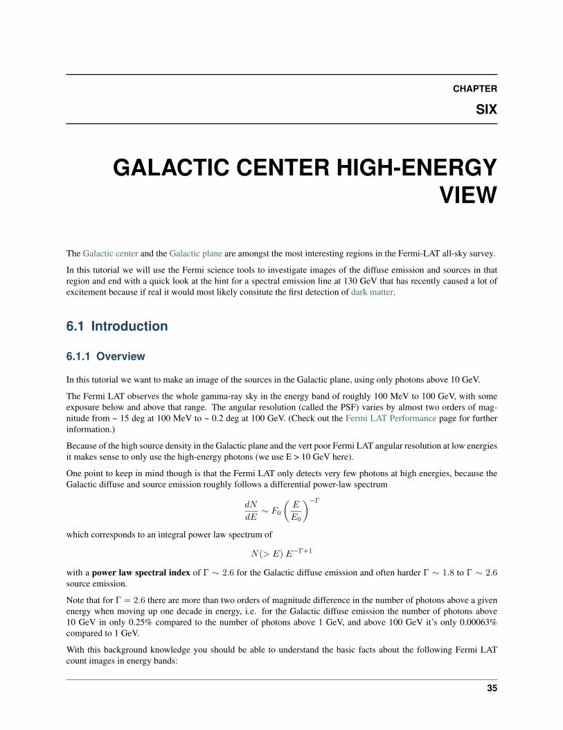
$ gtbin evfile=gtmktime.fits scfile=../../spacecraft.fits outfile=count_cube.fits \algorithm=CCUBE ebinalg=LOG emin=10e3 emax=316e3 enumbins=8 \nxpix=600 nypix=100 binsz=0.1 coordsys=GAL \xref=0 yref=0 axisrot=0 proj=CAR

$ gtexpcube2 infile=gtltcube.fits cmap=none outfile=gtexpcube2.fits \irfs=P7SOURCE_V6 nxpix=1800 nypix=900 binsz=0.2 coordsys=GAL \xref=0 yref=0 axisrot=0 proj=AIT \emin=10e3 emax=316e3 enumbins=8 bincalc=EDGE

$ gtmodel srcmaps=count_cube.fits srcmdl=diffuse_model.xml \outfile=model_image.fits irfs=P7SOURCE_V6 \expcube=gtltcube.fits bexpmap=gtexpcube2.fits

On my machine gtbin takes 5 seconds, gtexpcube2 takes 1 minute and gtmodel takes 5 minutes.

Note: Exercise: Inspect the generated files with ftlist and ds9 to see what they contain.

Consult the official Fermi LAT Binned Likelihood Tutorial analysis thread for detailed information.

6.4 Compute an excess and significance image with Python

We would like to compute correlated excess = counts - background and significance images of the sourcesdetected by the Fermi LAT above 10 GeV in the inner part of the Galactic plane, similar to the one we showedpreviously from the Fermi publication.

Note: What is statistical significance and how can I compute it?

6.4. Compute an excess and significance image with Python 39

fermi-hero Documentation, Release 0.1

TODO http://en.wikipedia.org/wiki/Statistical_significance

This functionality is not readily available as a command line Fermi Science Tool.

If would be possible to do it by using fgauss and ftimgcalc.

Instead of using these command line FTOOLs let’s use a Python script make_source_images.py:

1 """Compute correlated source excess and significance maps.2

3 Christoph Deil, 2013-09-124 """5 import numpy as np6 from numpy import sign, sqrt, log7 from scipy.ndimage import convolve8 import pyfits9

10 def correlate_image(image, radius):11 """Correlate image with circular mask of a given radius.12

13 This is also called "tophat correlation" and it means that14 the value of a given pixel in the output image is the15 sum of all pixel values in the input image within a given circular radius.16

17 https://gammapy.readthedocs.org/en/latest/_generated/gammapy.image.utils.tophat_correlate.html18 """19 radius = int(radius)20 y, x = np.mgrid[-radius: radius + 1, -radius: radius + 1]21 structure = x ** 2 + y ** 2 <= radius ** 222 return convolve(image, structure, mode=’constant’)23

24 def significance_lima(n_observed, mu_background):25 """Compute Li & Ma significance.26

27 https://gammapy.readthedocs.org/en/latest/_generated/gammapy.stats.poisson.significance.html28 """29 term_a = sign(n_observed - mu_background) * sqrt(2)30 term_b = sqrt(n_observed * log(n_observed / mu_background) - n_observed + mu_background)31 return term_a * term_b32

33

34 if __name__ == ’__main__’:35 print(’Reading count_image.fits’)36 counts = pyfits.getdata(’count_image.fits’)37 print(’Reading model_image.fits’)38 model = pyfits.getdata(’model_image.fits’)39

40 radius = 5 # correlation circle radius41 correlated_counts = correlate_image(counts, radius)42 correlated_model = correlate_image(model, radius)43

44 excess = correlated_counts - correlated_model45 significance = significance_lima(correlated_counts, correlated_model)46

47 header = pyfits.getheader(’count_image.fits’)48 print(’Writing excess.fits’)49 pyfits.writeto(’excess.fits’, excess, header, clobber=True)50 print(’Writing significance.fits’)51 pyfits.writeto(’significance.fits’, significance, header, clobber=True)

40 Chapter 6. Galactic Center High-Energy View

fermi-hero Documentation, Release 0.1

TODO: explain script a bit.

Run it by typing:

$ python make_source_images.py

Note: Exercise: Open up the exercise.fits and significance.fits images and see if the values roughlymake sense.

6.5 Explore Sources

Download the First Fermi-LAT Catalog of Sources above 10 GeV (1FHL) like this:

$ wget http://fermi.gsfc.nasa.gov/ssc/data/access/lat/1FHL/gll_psch_v07.fit

and the LAT 2-year Point Source Catalog in FITS and ds9 region format like this:

$ wget http://fermi.gsfc.nasa.gov/ssc/data/access/lat/2yr_catalog/gll_psc_v08.fit$ wget http://fermi.gsfc.nasa.gov/ssc/data/access/lat/2yr_catalog/gll_psc_v07.reg

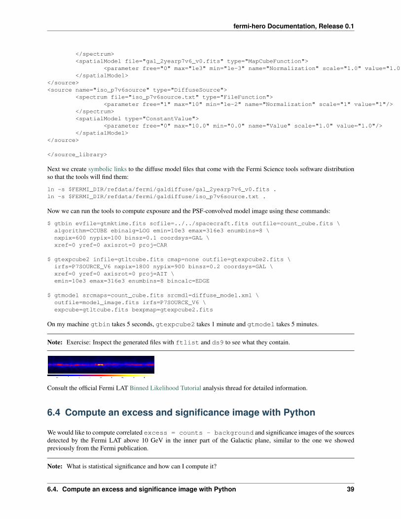
6.5.1 HESS Galactic plane survey

Figure 6.3: HESS survey image (TeV energy range). Reference: http://adsabs.harvard.edu/abs/2013arXiv1307.4690C

6.6 The 130 GeV line

6.6.1 What is it?

In April 2012 Christoph Weniger (not a member of the Fermi-LAT collaboration) reported “A tentative gamma-rayline from Dark Matter annihilation at the Fermi Large Area Telescope” (arXiv) with a statistical significance of 4.6sigma at 130 GeV, and 3.2 sigma after taking into account the look-elsewhere effect, i.e. the fact that he did search fora line in multiple regions of the sky and at multiple energies.

This generated a lot of noise in the gamma-ray astrophysics community because, if real, this 130 GeV gamma-rayemission line cannot easily be explained by normal astrophysical sources ... for almost all sources we expect fromtheory and also see power-law spectra ... sometimes with curvature or cutoff, but never with a sharp line feature.

On the other hand ... if the dark matter we know exists in the inner part of our Galaxy (all galaxies, actually) consistsof weekly interacting particles (Wimps), there are theories that predict them to annihilate and produce an emission lineconsistent with the feature discovered in the Fermi LAT data.

In May 2013 the Fermi LAT collaboration has reported their “Search for Gamma-ray Spectral Lines with the FermiLarge Area Telescope and Dark Matter Implications” (arXiv), computing the statistical significance of this line featureat 130 GeV at a lower statistical significance of 3.3 sigma, and only 1.6 sigma after taking the look-elsewhere effectinto account.

6.5. Explore Sources 41

fermi-hero Documentation, Release 0.1

You can find a nice summary and the latest results in this presentation by Andrea Albert at the recent TeVPA 2013conference if you don’t have time to read the 40-page paper.

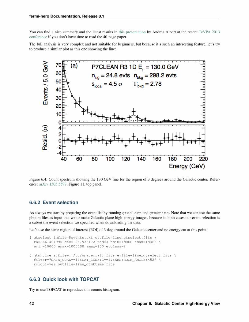
The full analysis is very complex and not suitable for beginners, but because it’s such an interesting feature, let’s tryto produce a similar plot as this one showing the line:

Figure 6.4: Count spectrum showing the 130 GeV line for the region of 3 degrees around the Galactic center. Refer-ence: arXiv 1305.5597, Figure 11, top panel.

6.6.2 Event selection

As always we start by preparing the event list by running gtselect and gtmktime. Note that we can use the samephoton files as input that we to make Galactic plane high-energy images, because in both cases our event selection isa subset the event selection we specified when downloading the data.

Let’s use the same region of interest (ROI) of 3 deg around the Galactic center and no energy cut at this point:

$ gtselect infile=@events.txt outfile=line_gtselect.fits \ra=266.404996 dec=-28.936172 rad=3 tmin=INDEF tmax=INDEF \emin=10000 emax=1000000 zmax=100 evclass=2

$ gtmktime scfile=../../spacecraft.fits evfile=line_gtselect.fits \filter="DATA_QUAL==1&&LAT_CONFIG==1&&ABS(ROCK_ANGLE)<52" \roicut=yes outfile=line_gtmktime.fits

6.6.3 Quick look with TOPCAT

Try to use TOPCAT to reproduce this counts histogram.

42 Chapter 6. Galactic Center High-Energy View

fermi-hero Documentation, Release 0.1

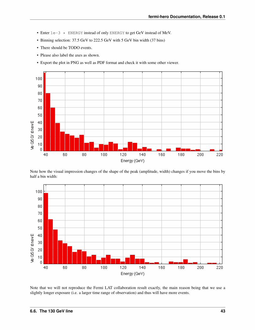
• Enter 1e-3 * ENERGY instead of only ENERGY to get GeV instead of MeV.

• Binning selection: 37.5 GeV to 222.5 GeV with 5 GeV bin width (37 bins)

• There should be TODO events.

• Please also label the axes as shown.

• Export the plot in PNG as well as PDF format and check it with some other viewer.

Note how the visual impression changes of the shape of the peak (amplitude, width) changes if you move the bins byhalf a bin width:

Note that we will not reproduce the Fermi LAT collaboration result exactly, the main reason being that we use aslightly longer exposure (i.e. a larger time range of observation) and thus will have more events.

6.6. The 130 GeV line 43

fermi-hero Documentation, Release 0.1

The Fermi plot has 24.8 + 298.2 = 323 according to the label. If you click Subsets -> New subset fromvisible in TOPCAT you will see that we have 412 events.

6.6.4 Nice plot with Python matplotlib

The Fermi science tools ships with two Python packages that you can use to make plots:

• ROOT can be used from Python like this: import ROOT

• matplotlib can be used from Python like this: import matplotlib.pyplot as plt

Note: In my opinion, the matplotlib import looks more complicated, but apart from that it is better documentedand easier to use and more powerful than ROOT plotting. But both have a learning curve ... we suggest you try outboth a bit, then stick with the one you like better.

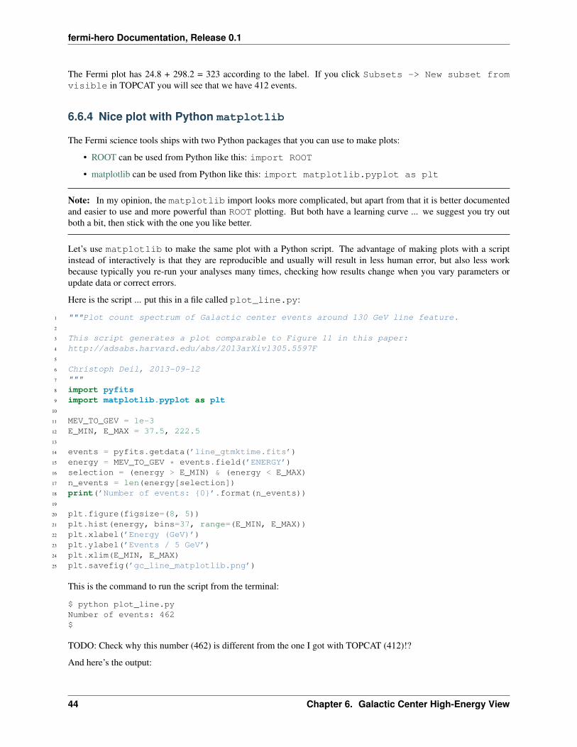
Let’s use matplotlib to make the same plot with a Python script. The advantage of making plots with a scriptinstead of interactively is that they are reproducible and usually will result in less human error, but also less workbecause typically you re-run your analyses many times, checking how results change when you vary parameters orupdate data or correct errors.

Here is the script ... put this in a file called plot_line.py:

1 """Plot count spectrum of Galactic center events around 130 GeV line feature.2

3 This script generates a plot comparable to Figure 11 in this paper:4 http://adsabs.harvard.edu/abs/2013arXiv1305.5597F5

6 Christoph Deil, 2013-09-127 """8 import pyfits9 import matplotlib.pyplot as plt

10

11 MEV_TO_GEV = 1e-312 E_MIN, E_MAX = 37.5, 222.513

14 events = pyfits.getdata(’line_gtmktime.fits’)15 energy = MEV_TO_GEV * events.field(’ENERGY’)16 selection = (energy > E_MIN) & (energy < E_MAX)17 n_events = len(energy[selection])18 print(’Number of events: {0}’.format(n_events))19

20 plt.figure(figsize=(8, 5))21 plt.hist(energy, bins=37, range=(E_MIN, E_MAX))22 plt.xlabel(’Energy (GeV)’)23 plt.ylabel(’Events / 5 GeV’)24 plt.xlim(E_MIN, E_MAX)25 plt.savefig(’gc_line_matplotlib.png’)

This is the command to run the script from the terminal:

$ python plot_line.pyNumber of events: 462$

TODO: Check why this number (462) is different from the one I got with TOPCAT (412)!?

And here’s the output:

44 Chapter 6. Galactic Center High-Energy View

fermi-hero Documentation, Release 0.1

6.6.5 Conclusion

So what do you think is the origin of the line feature?

Note that there’s a ~ 5% chance that the line is simply a Poisson background fluctuation. To compute this probabilityfrom the given significance you can use scipy.stats.norm, althogh for me currently the import fails with the FermiScienceTools Python:

$ ipython

In [1]: from scipy.stats import norm

In [2]: norm.sf(1.6)Out[2]: 0.054799291699557974

6.6. The 130 GeV line 45

fermi-hero Documentation, Release 0.1

46 Chapter 6. Galactic Center High-Energy View

CHAPTER

SEVEN

APERTURE LIGHTCURVE

7.1 Computing the aperture lightcurve

In this section of the tutorial we will learn how to generate an aperture lightcurve from Fermi/LAT.

There are two different kinds of lightcurves that can be computed from Fermi/LAT observations: using likelihoodanalysis on each of the lightcurve bins, or aperture analysis. The likelihood analysis leads to a better sensitivity and theability to obtain background-substracted flux lightcurves, but is model-dependent and very computationally intensive,especially for longer periods of time. Aperture lightcurve generation, on the other hand, is less computationallydemanding and provides a model-independent estimate of the variability of a given source. However, there is no wayto do an estimation of the background, so it should not be used to estimate the source’s flux.

Here we will compute the aperture lightcurve of the remarkable April 2011 flare from the Crab Nebula. The CrabNebula has been used for decades as the standard candle in High Energy Astrophysics, as it is bright and expected tohave a constant flux. However, Fermi/LAT discovered that its flux is far from constant, exhibiting flux changes of afactor of 10 or more over just a few hours. The astrophysical process behind these flares is still unkown.

Figure 7.1: Fermi/LAT lightcurve of the April 2011 Crab Nebula flare as published in Buehler et al. (2012), ApJ 749,26

In this tutorial we assume that you have already installed and initialized the Fermi Science Tools as well as enrico.

Change directory to where you have extracted the excercise data files and enter the lightcurve directory. You canexplore the data selection applied to the event file with gtvcut command.

Generate an configuration file for this observation with the command:

47

fermi-hero Documentation, Release 0.1

$ enrico_config crab.conf

and enter the name and coordinates of the source (you will find them in the data selection cuts shown with gtvcut).For the aperture lightcurve, the model and ROI size parameters are not used, so leave them to their default values.Finally, select the initial and final analysis times as given in the server query file.

You can the edit the file crab.conf to check the parameters. In addition to the target, space, file, andtime categories, the AppLC configuration category includes the values used by enrico when creating the aperturelightcurve. Use the NLCbin parameter to set the number of bins desired in the lightcurve between tmin and tmax.Given that the total selection time in the photon file is 16 days, 32 bins will result in a bin width of 12 hours, and64 bins in a bin width of 24 hours. You can try different bin widths to check which one yields the most informativelightcurve, taking into account that shorter time bin widths will result in larger uncertainties.

During these observations the survey mode of the Fermi observatory was changed in favour of pointed observa-tions towards the Crab Nebula. For this reason, one of the filter options in crab.conf (ABS(ROCK_ANGLE)<52)should be removed as it is related to the survey mode spacecraft rocking. The resulting filter expression in[analysis]/filter should be:

[analysis]filter = DATA_QUAL==1&&LAT_CONFIG==1

Finally, run the aperture lightcurve enrico script:

$ enrico_applc crab.conf

This scrip will run the following tasks:

1. gtselect : Select the events from the input FT1 file.

2. gtmktime : Compute good time intervals based on spacecraft pointing and SAA position.

3. gtbin : Bin the data into a lightcurve.

4. gtexposure : Compute the exposure (effective area*observation time) for each of the bins.

5. From the results of gtbin and gtexposure, lightcurve plots are generated in the AppertureLightcurvedirectory.

The resulting aperture lightcurve will be saved in AppertureLightcurve/AppLC.eps, and should reproducethe two peaks shown in Buehler et al. (2012) as seen in the following example:

48 Chapter 7. Aperture Lightcurve

fermi-hero Documentation, Release 0.1

7.1. Computing the aperture lightcurve 49

fermi-hero Documentation, Release 0.1

50 Chapter 7. Aperture Lightcurve

CHAPTER

EIGHT

MORE

Pointers to learn more gamma-ray data analysis ...

• http://python4astronomers.github.io

• https://astropy4mpik.readthedocs.org/en/latest/

• https://gammafit.readthedocs.org/en/latest/

Other Fermi LAT tutorials or useful links:

• http://adsabs.harvard.edu/abs/2013arXiv1307.4534S

• http://fermi.gsfc.nasa.gov/science/mtgs/summerschool/2013/program.html

• https://confluence.slac.stanford.edu/display/LSP/Fermi+Summer+School+2013

• http://nbviewer.ipython.org/urls/raw.github.com/kialio/fermi-summer-school/master/Data_Exploration.ipynb

• http://grbworkshop.wikidot.com/s6-fermi-lat-analysis-hands-on

• https://confluence.slac.stanford.edu/display/LSP/Installing+the+Virtual+Machine

• http://fermi.gsfc.nasa.gov/science/mtgs/workshops/da2012_solar/instructions.html

• http://www.asdc.asi.it/articles.php?id=52

• http://fermi.gsfc.nasa.gov/ssc/library/conferences/219aas/

51