Syracuse University Syracuse University SURFACE SURFACE Dissertations - ALL SURFACE May 2019 Relevant Operators of Particle Physics and Cosmology Relevant Operators of Particle Physics and Cosmology Cem Eroncel Syracuse University Follow this and additional works at: https://surface.syr.edu/etd Part of the Physical Sciences and Mathematics Commons Recommended Citation Recommended Citation Eroncel, Cem, "Relevant Operators of Particle Physics and Cosmology" (2019). Dissertations - ALL. 1035. https://surface.syr.edu/etd/1035 This Dissertation is brought to you for free and open access by the SURFACE at SURFACE. It has been accepted for inclusion in Dissertations - ALL by an authorized administrator of SURFACE. For more information, please contact [email protected].
Transcript
Syracuse University Syracuse University
SURFACE SURFACE
Dissertations - ALL SURFACE
May 2019
Relevant Operators of Particle Physics and Cosmology Relevant Operators of Particle Physics and Cosmology
Cem Eroncel Syracuse University
Follow this and additional works at: https://surface.syr.edu/etd
Part of the Physical Sciences and Mathematics Commons
Recommended Citation Recommended Citation Eroncel, Cem, "Relevant Operators of Particle Physics and Cosmology" (2019). Dissertations - ALL. 1035. https://surface.syr.edu/etd/1035
This Dissertation is brought to you for free and open access by the SURFACE at SURFACE. It has been accepted for inclusion in Dissertations - ALL by an authorized administrator of SURFACE. For more information, please contact [email protected].
Without a doubt, the Standard Model of Particle Physics (SM) can be considered as one
of the most significant victories of Theoretical High Energy Physics in the last century.
It provides the most accurate and complete description of fundamental particles and the
interactions between them. The last remaining piece of it, the Higgs boson, was finally
discovered in July 2012 at CERN [1, 2], thereby it has been verified up to the energy scale
and experimental accuracy that today’s collider technology can reach.
Despite of its success, the SM is not the final theory of fundamental interactions. In this
chapter, we will try to explain why this is the case. After a brief review of SM, we will argue
why SM should be treated as an Effective Field Theory (EFT). But we will see that this
treatment brings deep conceptual issues which arise due to existence of relevant operators.
Finally we will conclude this chapter with an outline of the dissertation.
1.1 Brief Review of the Standard Model
SM is a non-abelian gauge theory, with the gauge group given by SU(3)C ⊗ SU(2)L ⊗ U(1)Y .
These gauge symmetries describe three of the four known fundamental forces. The SU(3)C
group describes the strong force while the product group SU(2)L ⊗ U(1)Y describes the
weak force and electromagnetism unified at high energies. At low energies, this group is
1
spontaneously broken to a subgroup U(1)EM due to Higgs mechanism, and as a result the
electromagnetism and the weak force are portrayed as separate interactions.
Being a quantum field theory, the fundamental building blocks of the SM are quantum
fields, which are categorized in terms of their transformation properties under the SM gauge
group and the Lorentz group.
First category consists of gauge bosons, which are the necessary ingredients of a gauge
theory. These are spin-1 fields and they transform under the adjoint representation of the
corresponding gauge group. Physically, these fields are force carriers since the interactions
between matter particles are carried using them. The gauge fields corresponding to the
group SU(3)C are called gluons, while the ones corresponding to the group SU(2)L ⊗ U(1)Y
are called electroweak bosons. The number of gauge fields are determined by the dimension
of the representation. Since the dimension of the adjoint representations of the SU(N) group
is N2 − 1, there are 8 gluons and 4 electroweak bosons. With all these information, we can
write the Yang-Mills part of the SM Lagrangian in terms of the gauge field strengths as
LYM = − 1
4g23
8∑a=1
GaµνG
µνa
︸ ︷︷ ︸SU(3)C
− 1
4g2
3∑b=1
W bµνW
µνb
︸ ︷︷ ︸SU(2)L
− 1
4g′2BµνB
µν︸ ︷︷ ︸U(1)Y
, (1.1)
where g3, g and g′ are gauge coupling constants of SU(3)C , SU(2)L and U(1)Y respectively.
Second category contains the spin 1/2 fields, known as fermions. These fields are not
required in order to define a gauge theory, however they need to exist in the SM because
phenomenologically we know these particles do exist. They can be classified into two cate-
gories depending on whether they transform under the strong group SU(3)C or not. While
the quarks transform under SU(3)C , the leptons do not. Another classification can be made
according to their representations under the Lorentz group. Left-handed and right-handed
fermions transform in the(12, 0)
and(0, 1
2
)representation of the Lorentz group respectively.
For some unknown reason, the transformation of left and right-handed fermions under the
SU(2)L group are not the same. While the left-handed fermions transform in the fundamen-
2
tal representation, the right-handed fermions are singlets, i.e. they do not transform under
SU(2)L. On the other hand, all quarks transform under the fundamental representation of
the strong group SU(3)C .
Since the left-handed fermions are in the fundamental representation of SU(2)L, both
left-handed quarks and leptons need to be paired separately in doublets. Again for some
unknown reason, there are 3 copies of quark and lepton doublets, known as generations.
Thus, the left-handed fermion content of the SM can be described as
Li =
νeLeL
,νµLµL
,ντLτL
, Qi =
uLdL
,cLsL
,tLbL
, (1.2)
where i = 1, 2, 3 is the generation index. The right-handed fermions will be the singlet
versions of these states with the exception of neutrinos since no right-handed neutrino has
been observed so far. Thus the right-handed fermion content is given by
eiR = eR, µR, τR , uiR = uR, cR, tR , diR = dR, sR, bR. (1.3)
Then, the fermion kinetic terms in the SM Lagrangian are written by
LK = iLi /DLi + iQi /DQi + ieiR /DeiR + iuiR /Du
iR + idiR /Dd
iR, (1.4)
where /D ≡ γµDµ and Dµ is the gauge covariant derivative corresponding to the representa-
tion of the fermion and sum over the generation index i is assumed.
All the SM particles do transform under the U(1)Y group and their transformation prop-
erties under this group are determined by their hypercharges. Since U(1)Y is an abelian group,
in contrast to the SU(3)C and SU(2)L groups which are non-abelian, the hypercharges are
in general arbitrary real numbers. However in the SM they need to be rational numbers in
order that the SM is a consistent quantum field theory. More specifically, the hypercharges
need to be rational numbers satisfying some relations in order that the gauge anomalies do
3
SU(3)C SU(2)L U(1)Y
Gluons Ga8a=1 Ad 1 0
Electroweak bosons W a4a=1 1 Ad 0
Left-handed leptons Li3i=1 1 −12
Right-handed leptons eiR3
i=1 1 1 −1
Left-handed quarks Qi3i=1 16
Right-handed up-type quarks uiR3
i=1 1 23
Right-handed down-type quarks diR3
i=1 1 −13
Higgs H 1 12
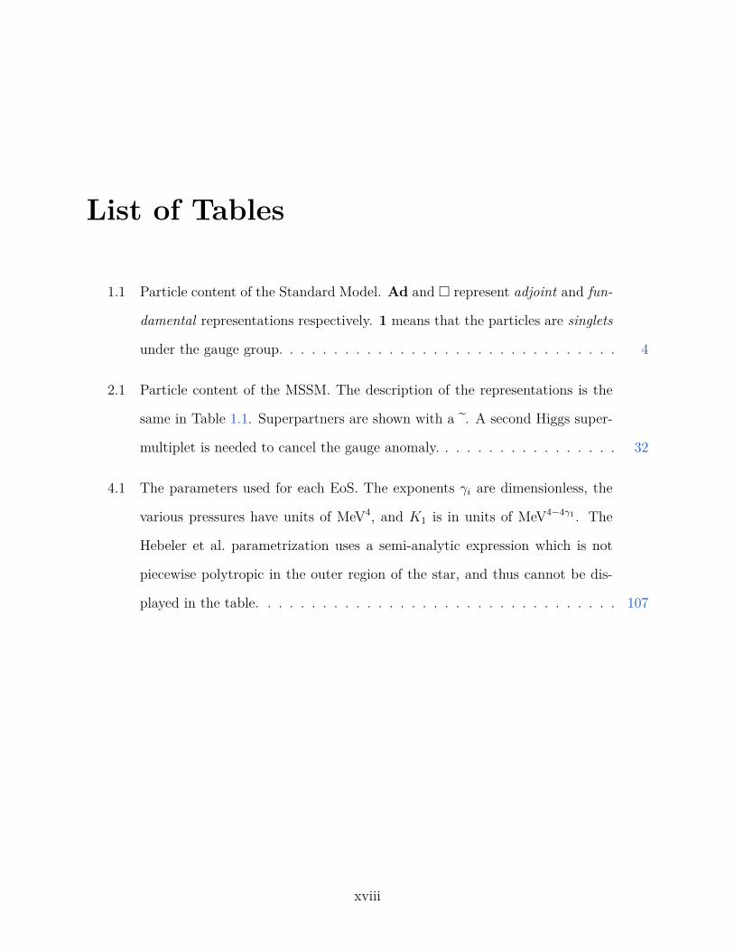
Table 1.1: Particle content of the Standard Model. Ad and represent adjoint and funda-mental representations respectively. 1 means that the particles are singlets under the gaugegroup.
vanish. The cancellation of gauge anomalies is a requirement for a consistent quantum field
theory, since otherwise unitarity will not be preserved and the theory will contain negative
norm states. The representations of the SM fields, plus the Higgs field which we will describe
soon, under the SM gauge group are shown in Table 1.1.
So far we did not include any mass term, although we know that all quarks and fermions,
as well as some gauge bosons, W± and Z, are massive. But we can’t write mass terms for
these particles explicitly, since these terms are not gauge invariant. This tells us that in order
to generate mass terms for the fermions and gauge bosons, the gauge symmetry needs to be
spontaneously broken. This phenomenon can be explained using the Higgs Mechanism [3–5].
In this mechanism, one adds to the SM field content a spin-0 complex scalar field multiplet
H, the Higgs field, which is a doublet under the SU(2)L and singlet under the SU(3)C . One
4
also assumes a potential for the Higgs given by
V (|H|) = −m2H |H|2 + λH |H|4, λH > 0. (1.5)
If m2H < 0, then this potential is clasically minimized at H = 0, hence the vacuum expectation
value (VEV) of the Higgs becomes 〈H〉 = 0. However, when m2H > 0 the Higgs acquires a
non-zero VEV given by 〈|H|〉 = mH√2λH
6= 0. This non-zero VEV spontaneously breaks the
SU(2)L ⊗U(1)Y symmetry into U(1)EM, which is the gauge group of electromagnetism. This
phenomenon is known as the electroweak symmetry breaking.
To see how the gauge bosons W± and Z get their masses, we should consider the full
electroweak Lagrangian including the Higgs:
LEW = −1
4W a
µνWµνa − 1
4BµνB
µν + (DµH)†(DµH)− V (|H|), (1.6)
where V (|H|) is given by (1.5). This is the Glashow-Weinberg-Salam model of electroweak
unification [6–8]. The coupling between the Higgs and the electroweak bosons arises due to
the gauge covariant derivative term which is explicitly given by
DµH = ∂µH − igW aµ τ
aH − 1
2g′BµH. (1.7)
In this expression τa are canonically normalized Pauli matrices, τa = 12σa, which are
the generators of SU(2) Lie algebra. W aµ , Bµ are electroweak gauge bosons, g and g′ are
SU(2)L and U(1)Y gauge couplings respectively, and 12
factor comes from the fact that the
Higgs doublet has hypercharge Y = 12. For a vanishing Higgs VEV, (1.6) reduces to the
Lagrangian of the pure SU(2)L ⊗ U(1)Y gauge theory with massless gauge bosons. However
if the Higgs gets a VEV, then we need to expand around this new vacuum. This can be done
5
by expanding the Higgs field after the symmetry breaking as
H = exp
2iπaτa
vH
0
1√2(vH + h)
, (1.8)
where vH = mH√λH
. The πa’s are the analog of the Nambu-Goldstone bosons (NGBs) which
arises due to spontaneous breaking of continuous global symmetries. The number of NGBs
is equal to the number of broken generators, so the breaking SU(2)L ⊗ U(1)Y → U(1)EM
introduces 4−1 = 3 NGBs. The field h is the massive excitation of the Higgs field H around
the new vacuum and it represents the Higgs particle.
The particle content after the symmetry breaking can be studied by substituting the
expansion (1.8) into the Lagrangian (1.6) and choosing the unitary gauge to set πa = 0.
Also some field redefinitions are needed to diagonalize the mass terms:
Zµ ≡ cos θwW3µ − sin θwBµ,
Aµ ≡ sin θwW3µ + cos θwBµ, (1.9)
W±µ ≡ 1√
2
(W 1
µ ∓ iW 2µ
)2,
where θw = g′
g. With these redefinitions, the kinetic and mass terms in (1.6) after the
symmetry breaking becomes
LEW→EM ⊃− 1
4FµνF
µν − 1
4ZµνZ
µν +1
2m2
zZµZµ
− 1
2
(∂µW
+ν − ∂νW
+µ
) (∂µW ν− − ∂νW µ−)+m2
WW+µ W
µ−
+1
2∂µh∂
µh− 1
2m2
hh2, (1.10)
where Fµν = ∂µAν − ∂νAµ, Zµν = ∂µZν − ∂ν − Zµ, and the mass terms are
mz =gvH
2 cos θw, mW =
gvH2
, mh =√2mH . (1.11)
6
We see that the W± and Z bosons which were massless before the electroweak symmetry
breaking now become massive, but the gauge boson Aµ, which corresponds to the photon,
remains massless. As shown by Eugene Wigner in 1939, the number of degrees of freedom
(DOF) of massive spin-s field is 2s + 1, while the number of DOF of any massless field is
2 [9]. Therefore, the massive gauge bosons should get a degree of freedom due to symmetry
breaking and it should come from the Higgs field. The three degrees of freedom that W±, Z
bosons need come from the NGBs πa. Thus we say that the NGBs are eaten by the gauge
bosons as a result of spontaneous symmetry breaking.
We will conclude this section by explaining how the fermions, more specifically charged
leptons and quarks, can get their masses. The SM fermions as shown in (1.2) and (1.3) are
2-component Weyl fermions, so they are by definition massless. In order to write a mass term
for a fermion, we need to mix left-handed and right-handed Weyl fermions. For instance,
a mass term for the electron will be of the form eLeR. The problem is that such a term
does break SU(2)L, so it is not allowed by gauge invariance. This shows that, just as the
massive gauge bosons, the fermions need to get their masses by the Higgs mechanism. In
order this to happen, they need to couple to the Higgs field. This can be accomplished by
adding Yukawa terms to the SM Lagrangian. For charged leptons we need to add
LLYuk = −
∑i=e,µ,τ
yiLiHeiR + h.c. (1.12)
where yi are Yukawa couplings. Quark masses can be generated similarly by
LQYuk = −
3∑i,j=1
(Y dijQ
iHdjR + Y uij Q
iHujR
)+ h.c. (1.13)
where H ≡ iσ2H∗. In this expression, the first term generates masses for the quarks d, s, b,
while the second term generates for the quarks u, c, t. After the symmetry breaking, the
Higgs field H will be replaced by its VEV, H → mH√2λH
= vH√2. Then (1.12) generates mass
7
terms for the charged leptons. As an example, the mass term for the electron will be
−me(eLeR + eReL), with me =yevH√
2. The Yukawa terms for the quarks (1.13) become after
the symmetry breaking
LQYuk = − v√
2
(dLY
ddR + uLYuuR
)+ h.c. (1.14)
where now Y d and Y u are 3× 3 complex matrices with elements(Y u,d
)ij= Y u,d
ij . To obtain
the quark masses, the mass terms in (1.14) need to be diagonalized. This can be achieved
by introducing two diagonal matrices Md and Mu and two unitary matrices Ud and Uu so
that
YdY†d = UdM
2dU
†d and YuY
†u = UuM
2uU
†u. (1.15)
One can further write
Yd = UdMdK†d and Yu = UuMuK
†u, (1.16)
where Kd and Ku are again unitary matrices. Then, after a change of basis by uL → UuuL,
dL → UddL, dR → KddR and uR → KuuR, (1.14) in the mass basis becomes
LQYuk = −
3∑i
(md
i diLd
iR +mu
i uiLu
iR
)+ h.c. (1.17)
wheremd
i
and mu
i are the diagonal elements of v√2Md and v√
2Mu respectively.
This concludes our lightning review of the SM. In the next section we will discuss why
we expect that this picture should change eventually.
8
1.2 The Standard Model as an Effective Theory
The SM is being tested continuously in collider experiments with ever-increasing precision.
So far, no statistically significant deviation have been measured1. Despite of this, we know
that there should exist physics beyond the SM since there are a lot of physical phenomena
which cannot be explained using the framework of SM. Some of the notable ones are
• Neutrino Masses: Neutrinos are massless in the SM. Writing mass terms for them
using the Yukawa interactions like in (1.12) is not possible because right-handed neu-
trinos do not exists in the field content of the SM; at least they have not been observed.
But, we have learned from neutrino oscillations experiments that they do have a tiny
but non-zero mass.
• Dark Matter: Latest cosmological observations show that the SM fields can only
provide 15% of the matter in the observable universe [15]. The rest of it consists
of a hypothetical substance called dark matter. If it is a particle, then it should be
electrically neutral, weakly interacting and stable to explain all the observations. The
SM does not have such a candidate.
• Dark Energy: The supernova observations made in 1998 showed that the universe is
not only expanding but the expansion is accelerating [16,17]. The most commonly used
cosmological model for explaining both dark matter and dark energy is ΛCDM model
which contains cold dark matter and a positive cosmological constant term. Attempting
to derive this term using the SM leads to a 120 order of magnitude discrepancy known
as the cosmological constant problem. We shall explore this further later in this chapter.
• Matter-antimatter Asymmetry: Our observable universe contains vastly more
matter than antimatter although there is no reason that the universe should start in an1They are some experimental anomalies such as the proton radius puzzle [10], anomalous magnetic dipole
moment muon [11] and B-meson decays [12–14]. But it is still uncertain that these anomalies definitelycontradicting the SM.
9
asymmetric state. Hence, there should be a process which occurred in the early universe
and produced this asymmetry. Such a process is not possible with the ingredients of
the SM [18].
In addition to all these missing pieces, the strongest hint for the incompleteness of the SM
comes from the fact that an UV complete quantum description of gravity is missing in the
SM. The phrase UV complete is crucial for the validity of this statement, since an effective
description of quantum gravity is perfectly compatible with the SM and even provide testable
predictions. To arrive such a description, we start with the fact that the graviton, which is
the force carrier of the gravity, should be a massless spin-2 field. Then using the requirements
of unitarity and Lorentz invariance, it is possible to show that the unique Lagrangian one
can write is [19]
Lg =M2pl
√− det
(ηµν +
1
Mplhµν
)R(ηµν +
1
Mplhµν
), (1.18)
where hµν represents the fluctuations of the metric, i.e. gµν = ηµν +M−1pl hµν , Mpl = G
−1/2N ≈
1019GeV with GN being the Newton’s constant, and R is the Ricci scalar. The scale Mpl
has been introduced so that the graviton field hµν has mass dimension one. This is precisely
the Einstein-Hilbert Lagrangian of general relativity. This shows that the Lagrangian for
general relativity is the unique Lagrangian that can couple a spin-2 field to matter.
If this construction works so well, why do we say that the description of quantum gravity
in the SM is not complete? The answer is related to the strength of the gravitational
interaction. If we expand the Lagrangian (1.18) we find
Lg ∼1
2hh+
1
MPlh3 +O
(1
M2pl
). (1.19)
We see that the gravitational interaction term h3 has the coupling constant M−1pl which has
negative mass dimension. Same situation will happen if we want to couple gravity to the SM
10
particles. As a spin-2 field, graviton should couple to the stress-energy tensor corresponding
to the SM
T µνSM = − 2√
−gδSSM
δgµνwith SSM =
∫d4x
√gLSM, (1.20)
and just from dimensional analysis the coupling should be of the form
1
MplhµνT
µνSM. (1.21)
The fact that the gravity coupling has negative mass dimension makes this description of
gravity perturbatively non-renormalizable. In these kind of field theories, one needs infinite
number of counterterms to cancel all the infinities arising from the loop corrections to the
model parameters. Despite of this difficulty, this description of gravity is perfectly valid and
even predictive, as long as the energy scale E we are probing is much smaller than the Planck
scale, E Mpl. In other words, the Lagrangian (1.19) together with the coupling (1.21)
provides an effective theory description of quantum gravity valid up to the cutoff scale Mpl
of the theory.
The breakdown of perturbative renormalizability does not mean that a field theory is ill-
defined at higher energies. Such a field theory might be non-perturbatively renormalizable, if
the Renormalization Group (RG) evolution of its couplings having negative mass dimensions
have non-trivial fixed points in the UV. Such theories are called asymptotically safe [20]. It
is a possibility that the gravity is such a theory, and this description holds even at higher
energies [21].
However, from a historical perspective, non-renormalizable theories were generally signs
of new physics and the cutoffs of these theories gave good estimates about the scale at which
new physics appeared. The most well known example of a non-renormalizable theory is the
Enrico Fermi’s theory β-decay [22]. In this theory, the weak decays are modeled using a
11
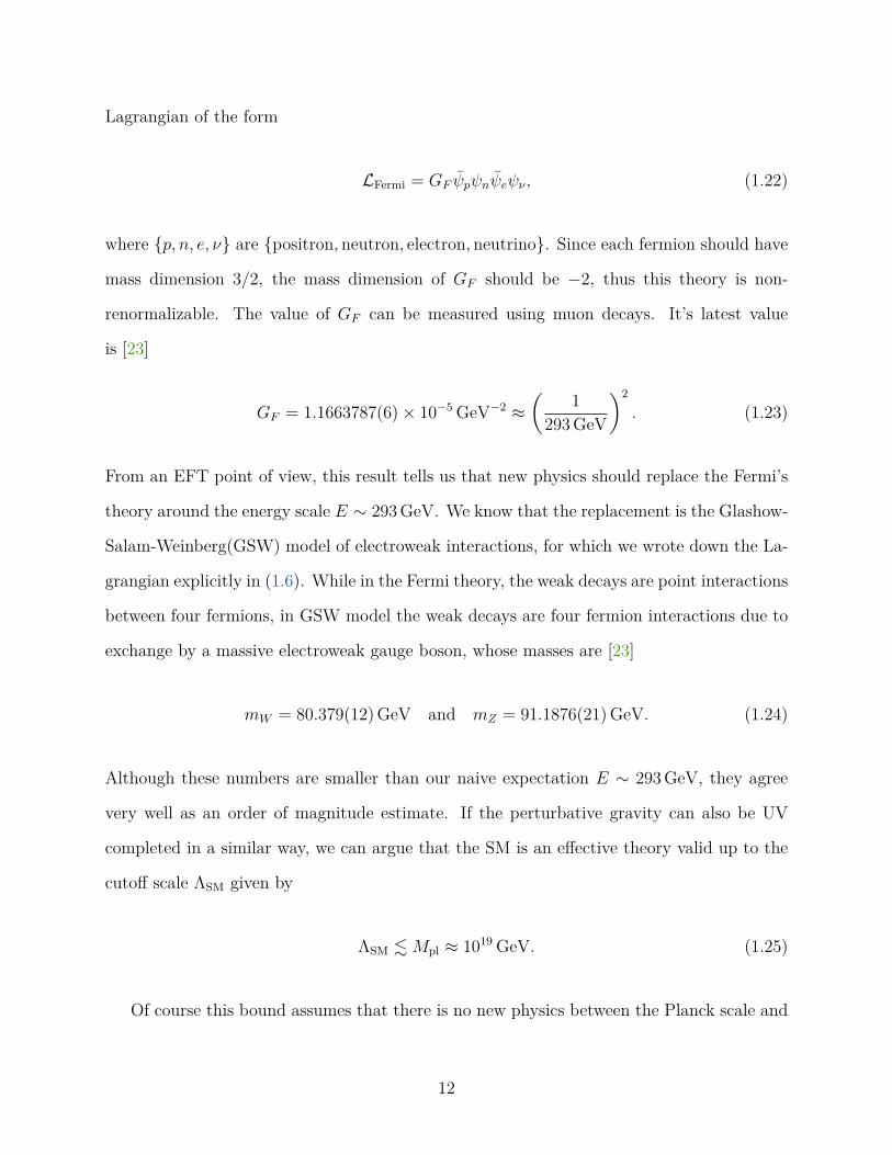
Lagrangian of the form
LFermi = GF ψpψnψeψν , (1.22)
where p, n, e, ν are positron, neutron, electron, neutrino. Since each fermion should have
mass dimension 3/2, the mass dimension of GF should be −2, thus this theory is non-
renormalizable. The value of GF can be measured using muon decays. It’s latest value
is [23]
GF = 1.1663787(6)× 10−5GeV−2 ≈(
1
293GeV
)2
. (1.23)
From an EFT point of view, this result tells us that new physics should replace the Fermi’s
theory around the energy scale E ∼ 293GeV. We know that the replacement is the Glashow-
Salam-Weinberg(GSW) model of electroweak interactions, for which we wrote down the La-
grangian explicitly in (1.6). While in the Fermi theory, the weak decays are point interactions
between four fermions, in GSW model the weak decays are four fermion interactions due to
exchange by a massive electroweak gauge boson, whose masses are [23]
mW = 80.379(12)GeV and mZ = 91.1876(21)GeV. (1.24)
Although these numbers are smaller than our naive expectation E ∼ 293GeV, they agree
very well as an order of magnitude estimate. If the perturbative gravity can also be UV
completed in a similar way, we can argue that the SM is an effective theory valid up to the
cutoff scale ΛSM given by
ΛSM .Mpl ≈ 1019GeV. (1.25)
Of course this bound assumes that there is no new physics between the Planck scale and
12
the energy scale being probed by today’s colliders, which is ∼ TeV. It is perfectly possible, in
fact expected, new physics will show up well before the Planck scale. In this case the cutoff
scale of the SM will be much lower than (1.25). Whenever the new physics scale appears,
and how complicated the new physics will be, it should be possible to express its effects in
energies E ΛSM by adding non-renormalizable operators to the SM Lagrangian. Hence to
study new physics, we can expand the SM Lagrangian generically as
LSM → LSM +∞∑
∆=5
1
Λ∆−4SM
O∆, (1.26)
where the mass dimension of the operator O∆ is [O∆] = ∆2.
The higher-dimensional operators O∆ are commonly used in attempts to explain the
problems of the SM we have mentioned before. For example, to generate neutrino masses
without right-handed neutrinos3, one can use the 5-dimensional Weinberg operator [24]
1
ΛSM
(LH)(
LcH), (1.27)
where Lc is the charge conjugate of the lepton doublet. This is the unique ∆ = 5 term
which can be written in the SM Lagrangian. With order one coefficients, this term generates
neutrino masses around mν ∼ 0.1 eV for ΛSM ≈ 1014GeV [25]. This example shows that the
EFT picture allows us to get hints about where the new physics might appear, even though
we don’t know the details of the new physics.
If we push ourselves to consider a situation where the SM does not get any corrections up
to the Planck scale and breakdown of perturbative renormalizability of quantum gravity is
saved by the asymptotic safety, there is still a problem which might prevents SM from being
a UV complete theory. The problem is with the RG evolution of the U(1)Y hypercharge2By mass dimension we mean canonical dimension, i.e. we are ignoring anomalous mass dimensions.3With right-handed neutrinos, neutrino masses can be generated with ∆ = 4 operators.
13
gauge coupling g′. At one loop, the RG evolution of g′ is given by [26]
4π
α1(E2)=
4π
α1(µ2)− 41
10log
(E2
µ2
), (1.28)
where
α1 =1
4π
5
3g′2 =
5α
3 cos2 θw, (1.29)
with α being the fine structure constant. The µ2 is an energy scale at which the coupling
constant α1 needs to be measured experimentally. We can see that due to the negative sign
of the log-term in (1.28), which corresponds to a positive β-function coefficient, there is an
energy scale ΛL at which the coupling constant diverges. This scale is given by α−11 (ΛL) = 0
or
4π
α1(µ2)=
41
10log
(Λ2
L
µ2
). (1.30)
Using the fact α(m2W ) ≈ 1/128 and sin2 θw(m
2Z) ≈ 0.231 [23], we get α1(m
2Z) ≈ 0.017 and
ΛL ∼ 1041GeV. (1.31)
This is called the Landau pole related to the U(1)Y gauge coupling and represents the break-
down of predictability of the SM as a perturbative field theory. One might worry that the
one-loop expression (1.28) is derived using perturbation theory but close to the Landau pole,
the gauge coupling g′ becomes non-perturbative and the one-loop expression looses its va-
lidity. In fact the lattice simulations of Quantum Electrodynamics (QED), which has the
similar problem albeit at Λ ∼ 10277GeV, show that before reaching to its Landau pole the
theory enters to a new phase at which fermions form a condensate and breaks the chiral
symmetry [27–29]. But such a condensate will also break the electroweak symmetry at a
14
much higher scale than the weak scale which will be in conflict with the GSW model we
have described in Section 1.1.
The take-away message of this section should be that although there is no mathematically
rigorous argument which proves that the SM is incomplete, there are a lot of hints, both
from theoretical and experimental point of view. In the rest of this dissertation, we will take
the SM as an EFT with some cutoff scale ΛSM as our starting point, and study what kind
of hints can we get from this effective description about the physics beyond the SM.
1.3 The Relevant Operator of the Standard Model and
the Hierarchy Problem
In the previous section we have argued that a good starting point for studying the beyond
the SM physics is an effective description of the SM with up to some cutoff scale ΛSM. This
cutoff scale should not be very close to the electroweak scale mW , since the current version
of the SM can reproduce the results of the collider experiments perfectly. We don’t know the
precise value for this cutoff, but it is pretty likely that the SM will be replaced by something
else at latest at the Planck scale, so for definiteness we choose ΛSM .Mpl.
Theories with a physical cutoff can be studied using the framework of Wilsonian renor-
malization group [30–34]. In contrast to the continuum RG picture where Λ stands for an
UV regulator which renders the loop integrals finite, the Wilsonian RG treats Λ as a refer-
ence scale of the theory, like atomic spacing in a metal. The RG evolution of the coupling
constants can be obtained by reducing the cutoff from Λ to Λ′, where one integrates out the
degrees of freedom Λ′ < p < Λ, and adjusting the coupling constants so that the low-energy
physics is the same.
In the Wilsonian RG and the EFT language, the operators are classified according to
their mass dimensions. If d denotes the number of spacetime dimensions and ∆ denotes
mass dimension of the operator, then the operator is called relevant if ∆ < d, irrelevant if
15
∆ > d, and marginal if ∆ = d. Classically marginal operators can get anomalous dimensions
from quantum corrections and depending the sign of the correction they can be relevant or
irrelevant, marginally so if the quantum corrections are small. If C∆−d is the (in general
dimensionful) coefficient of an operator of mass dimension ∆, then it can be shown that
under a RG transformation Λ → Λ′ = bΛ with b < 1, C∆−d scales as [35]
C∆−d → C ′∆−d = b∆−dC∆−d. (1.32)
Therefore for an irrelevant operator C ′ < C so the coupling of this operator decreases to-
wards lower energies, or towards IR, which implies that at lower energies E Λ this operator
becomes less important. We note that the irrelevant operators correspond to the perturba-
tively non-renormalizable terms in the Lagrangian. This explains why non-renormalizable
field theories are perfectly valid and predictive as low energy effective field theories.
On the other hand for a relevant operator C ′ > C and the coupling increases towards IR.
This implies that the relevant operators are sensitive to the UV physics. This immediately
rings an alarm bell. Our aim was to consider the SM as an effective theory with the hope
that its low-energy description will be independent of its UV completion, but we ended up in
a situation where the UV sensitivity of our model increases as we go to lower energy scales.
We would have been fine if the SM did not contain any relevant operators, but this is not
the case. There is only one relevant operator in the SM4, which is the Higgs mass parameter
in the Higgs potential (1.5). This is the essence of the so called hierarchy problem which we
will describe in detail now.
In (1.26), we added irrelevant operators to the Lagrangian by the terms of the form
Λ−(∆−4)SM O∆ with ∆ > 4. By extrapolating this form to the relevant operators we can argue
4Here we mean “relevant” by naive power counting. There are also marginally relevant operators in theSM, like the QCD field strength squared.
16
that the Higgs mass term should be of the form
cΛ2SM|H|2, (1.33)
where c is a dimensionless coefficient. We can see this formally by calculating the quantum
corrections to the Higgs mass parameter of (1.5). These corrections will come from Higgs
self-interactions, gauge and fermion loops. All these contributions are quadratically divergent
so they need to be regulated with a cutoff. Since we are treating the SM as an effective theory,
we can use ΛSM to regulate the integrals. Then we can express the quantum corrections to
the Higgs mass parameter as
δm2H ≈ Λ2
SM16π2
[−6y2t +
1
4
(9g2 + 3g′2
)+ 6λH + · · ·
], (1.34)
where yt is the top-quark Yukawa coupling5. Thus we see although we would have chosen a
small value for the bare Higgs mass parameter m2H , the quantum corrections will push it all
the way to the cutoff scale.
Of course the bare mass parameter is not an observable and we have to choose it such
that m2H + δm2
H reproduces the experimentally measured value for the Higgs mass, which
can also be defined as the pole mass. Since the Higgs pole mass is mh ≈ 125GeV, using
(1.11) we get (m2H)pole ≈ (88GeV)2. Choosing the SM cutoff ΛSM to be the Planck scale Mpl
we find
(m2H)pole = (m2
H)bare + δm2H ⇒ (88GeV)2 ≈ (m2
H)bare +(1019GeV
)2, (1.35)
where (m2H)bare is the bare mass parameter in the Higgs potential. This result shows that
5We have ignored the contribution from other fermions since they will be small compared to the top-quarkcontribution.
17
the bare mass parameter should be tuned to a precision of
(m2H)pole
Λ2SM
≈ (88GeV)2
(1019GeV)2∼ 10−34. (1.36)
This is called fine-tuning which means extreme sensitivity of the physical observables, such
as the Higgs pole mass, to variation of model parameters. The theories which require such
a precise tuning are usually called fine-tuned or unnatural.
Since the quadratic sensitivity to the cutoff scale in (1.35) comes from an UV divergent
integral, it is a meaningful question to ask what would have happened if we had choose a dif-
ferent regularization scheme to perform the loop integrals. A commonly used regularization
scheme in gauge theories is the dimensional regularization since it respects gauge invariance.
If one evaluates the loops in (1.34) using dimensional regularization, then one finds that the
quadratic divergence is replaced by a pole at ε = 0 with d = 4− ε
(δm2H)DimReg ∼ 1
ε+ finite. (1.37)
As in the usual renormalization procedure, this pole can be canceled by introducing suitable
counterterms and so one finds that the quantum correction to the Higgs mass is finite and
does not depend on the cutoff ΛSM at all.
At this point, one might think that the quadratic sensitivity to the cutoff scale in (1.34) is
merely a consequence of choosing a wrong regulator, therefore it does not represent something
physical. However from an effective field theory point of view, the Λ2SM in (1.34) not a
regulator, it is a physical scale which is a placeholder for new physics. Now we will show this
explicitly using a toy model6. We consider a theory given by the Lagrangian
L =1
2∂µφ∂
µφ− 1
2m2φ2 +
λ
4φ4 + iΨ(/∂ −M)Ψ + yφΨΨ, (1.38)
6The following discussion is based on the lectures given by Nathaniel Craig at the Prospects in TheoreticalPhysics (PiTP) 2017 summer school available at https://www.youtube.com/watch?v=orCZeoQXXWw.
where a scalar field φ is coupled to a fermion Ψ with a Yukawa interaction. We assume that
the mass of the scalar is much smaller than the fermion mass, so m M . In this case, we
consider an EFT with only the scalar field φ, where the heavy fermion Ψ has been integrated
out. The Lagrangian in the effective theory is
LEFT =1
2Zφ∂µφ∂
µφ− 1
2m2φ2 + · · · , (1.39)
where Zφ is the wave-function renormalization term and m2 is the renormalized mass param-
eter. We didn’t include the φ4 term since we only interested in the corrections that the mass
parameter will get. Now we want to perform a matching procedure between the full theory
and the effective theory at the scale M . This can be done by matching the scalar two-point
functions in both descriptions. At one loop, this matching can be done by calculating the
one-loop contribution involving the heavy fermion7:
To avoid any confusion with quadratic divergences, we will use the dimensional regularization
with minimal subtraction (MS) scheme to evaluate this loop. Then the contribution of this
loop to the scalar self-energy is given by
Σ2(p2) =
4y2
16π2
[(3
ε+ 1 + 3 log
(µ2
M2
))(M2 − p2
6
)+p2
2− p2
20M2+ · · ·
], (1.40)
where ε−1 = ε−1 − γE + log(4π) with γE being the EulerMascheroni constant. Then we
perform the renormalization procedure by adding counterterms to cancel the 1/ε pole and7The Feynman diagrams in this thesis are produced by the TikZ-Feynman package [36]
19
match at the scale µ =M . After this we find the Lagrangian in the effective theory as
LEFT =
(1− 4
3
y2
16π2
)1
2∂µφ∂
µφ−(m2 − 4y2
16π2M2
)1
2φ2 + · · · . (1.41)
We see that the scalar mass gets quantum corrections proportional to M2. This toy model
clearly demonstrates that the quadratic divergence in (1.34) is really a placeholder for new
physics. The hierarchy problem is not about quadratic divergences. It is about the sensitivity
to higher energy scales.
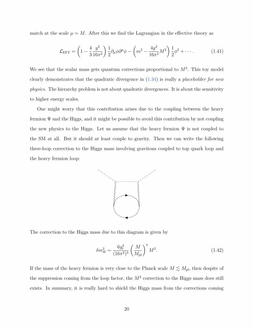
One might worry that this contribution arises due to the coupling between the heavy
fermion Ψ and the Higgs, and it might be possible to avoid this contribution by not coupling
the new physics to the Higgs. Let us assume that the heavy fermion Ψ is not coupled to
the SM at all. But it should at least couple to gravity. Then we can write the following
three-loop correction to the Higgs mass involving gravitons coupled to top quark loop and
the heavy fermion loop:
The correction to the Higgs mass due to this diagram is given by
δm2H ∼ 6y2t
(16π2)3
(M
Mpl
)4
M2. (1.42)
If the mass of the heavy fermion is very close to the Planck scale M .Mpl, then despite of
the suppression coming from the loop factor, the M2 correction to the Higgs mass does still
exists. In summary, it is really hard to shield the Higgs mass from the corrections coming
20
from the higher energy scales.
Before concluding this section, we will mention yet another way to describe the hierarchy
problem, which will make use of the symmetries. We have said that the hierarchy problem
is unique to the Higgs, since it is the only relevant operator in the SM. But there is another
reason why the Higgs suffers from this problem. To see this, consider the Lagrangian for
Quantum Electrodynamics (QED):
LQED = −1
4FµνF
µν + ψ(i /D −me
)ψ, (1.43)
with Dµψ = ∂µψ + ieAµψ. Here, ψ is the electron represented as a Dirac fermion and me
is the electron mass. The electron mass term looks like a relevant parameter so naively
we expect the quantum corrections will push it to higher scales. But if we calculate the
corrections we will find
δme =3αem
2πme log
(Λ
me
), (1.44)
where αem is the fine-structure constant. We see that the quantum corrections are propor-
tional to the electron mass itself, and instead of a quadratic divergence we get a much weaker
logarithmic divergence. To appreciate how much weaker it is, let us imagine an alternative
universe where the QED holds up to the Planck scale. Then taking Λ ∼ Mpl, αem ≈ 1/137
and me ≈ 0.511MeV we find
δme
me
∼ 0.2. (1.45)
What is the reason behind the logarithmic dependence in (1.44)? The answer is the
symmetry. If we set the electron mass me to zero in (1.43), the electron gains an additional
symmetry, namely the symmetry under axial transformations of the form ψ → eiαγ5ψ. In
other words, setting the electron mass to zero enhances the symmetry of the theory. Since in
21
this case the symmetry will also be respected by quantum corrections8, the corrections to the
mass parameter should be proportional to the mass parameter itself. Then by dimensional
analysis, we can conclude that the cutoff Λ can only appear inside the logarithm. In such a
scenario, one usually says that the electron mass is protected by the chiral symmetry.
The same situation happens with the Yukawa couplings in the SM. Setting them to zero
enhances the symmetry of the SM, so they are insensitive to higher energy scales. Therefore
the hierarchy between various Yukawa couplings, such as ye/yt ∼ 10−5, is not considered
to be a hierarchy problem. It is still a puzzle why such a hierarchy exists, but if it can
be explained in a UV completion of the SM, then that explanation will remain valid at
low energies too. Introducing a symmetry which protects the Higgs mass from quadratic
divergences is the most commonly used strategy in attempts to solve the hierarchy problem,
which we will briefly mention in Chapter 2.
1.4 A Relevant Operator of Cosmology and the Cos-
mological Constant Problem
When we wrote down the potential for the Higgs in (1.5), we didn’t include a constant term
V0. Such a term does not have any effect in particle physics, but it plays a big role in
cosmology. Although this term does not couple to any SM field, it will couple to gravity. If
we denote the VEV of Higgs by φh =√2 〈|H|〉, then the energy density of the vacuum will
be given by
⟨T 00
⟩≡ ρV = V (φh) = V0 −
m4H
λH. (1.46)
8Actually the chiral symmetry is anomalous so quantum corrections will introduce a term of the form FFwhere Fµν = εµνρσF
ρσ. But in the case of QED the FF term is a total derivative so it does not contributeto the equation of motion.
22
We see that the energy density of the vacuum is dependent on the choice of V0. The Einstein
equations with the cosmological constant term is given by
Rµν −1
2gµνR+ Λgµν =
8π
M2plTµν , (1.47)
where Λ is the cosmological constant. From this expression we can see that the vacuum energy
density ρV contributes to the cosmological constant term, giving an effective cosmological
constant expressed as
Λeff = Λ+8π
M2PlρV . (1.48)
So total effective vacuum energy of the universe is given by
〈ρ〉 = ρV + ΛM2
pl
8π= Λeff
M2pl
8π. (1.49)
This value can be measured using cosmological observations: [16, 17,37–41]
Λeff ∼ 10−52m−1 (1.50)
which corresponds to a vacuum energy density of
〈ρ〉 ∼ (10−12GeV)4. (1.51)
We shall see now that the smallness of this value results in a fine-tuning problem which
is much worse compared to the hierarchy problem. In the expression of the effective vacuum
energy (1.49), all the terms were classical contributions. There will also be quantum correc-
tions to the vacuum energy. If we consider SM with the cutoff ΛSM, then the sum of the
23
zero-point energies of all normal modes of some field of mass m will be given by
∫ ΛSM
0
d3k
(2π)31
2
√k2 +m2 ≈ Λ4
SM16π2
. (1.52)
Notice that, this is in agreement with our expectation from the effective field theory point
of view. The constant term in the Higgs potential V0 is a ∆ = 0 operator, therefore it
should appear in the effective theory as cΛ4V0, where c is a coefficient and Λ is the cutoff.
Again choosing the SM cutoff to be the Planck scale we find the natural value of the vacuum
energy density should be 〈ρ〉 ∼ M4pl. Comparing with the experimentally measured value
(1.51) implies a tuning of
(10−12GeV)4
M4pl/(16π
2)∼ 10−122. (1.53)
This is called the cosmological constant problem. It is the question of what kind of physical
process could have cancelled the enourmous contribution coming from the zero-point energies
of the quantum fields, such that the observed cosmological constant is very small.
The cosmological constant problem becomes much more interesting when we consider the
phase transitions in the early universe. The potential we wrote for the Higgs field in (1.5) is
at zero temperature. Since the temperature of the universe is very small today, T ∼ 3K, the
zero temperature description is adaquate for studying the phenomena happening at present
times. But at the early stages of the universe, the temperature was very high and one cannot
rely on a zero temperature description. The physics of the early universe can be studied using
finite-temperature field theory. In this framework, the classical potential V (φh) is replaced
by the finite-temperature effective potential, which is the free energy density associated with
the φh field. It can be expressed by
VT (φh) = ρφ − Tsφ, (1.54)
24
where ρφ is the energy density and sφ = −∂VT (φh)/∂T is the entropy density. To one loop in
quantum and thermal corrections, the finite-temperature effective potential VT (φh) is given
by [42,43]
VT (φh) = V1(φh) +T 4
2π2
∫ ∞
0
dxx2 log
[1− exp
−√x2 +
M2
T 2
], (1.55)
where M2(φh) = −m2H + 3λHφ
2h and V1(φh) is the zero-temperature potential including one
loop quantum effects
V1(φh) = V0 −1
2m2
Hφ2h +
1
4λHφ
4h +
M4
64π2log
(M2
µ2
), (1.56)
with µ being an arbitrary renormalization scale. The integral in (1.55) can be expanded in
M2/T 2 to get
VT (φh) = V1(φh)−π2
90T 4 +
M2
24T 2 + · · · . (1.57)
Then using (1.56) we obtain
VT (φh) =
(V0 −
π2
90T 4 − m2
H
24T 2
)+
(λH8T 2 − 1
2m2
H
)φ2h +
λH4φ4h + · · · , (1.58)
whereV0, mH , λH
represent one-loop renormalized model parameters of the zero-temperature
Higgs potential. From this expression we see that for m2H > 0, the coefficient of the φ2
h term
changes sign at a critical temperature Tc given by
Tc ≈2mH√λH
. (1.59)
Therefore the electroweak symmetry, which is broken at zero temperature, was unbroken
when the temperature of the universe was higher than this critical temperature. Precise
determination of this value requires the knowledge of the renormalized model parameters,
25
but as an order of magnitude estimate we can accept Tc ∼ 100GeV ∼ mEW, where mEW is
the electroweak scale.
Now, let us investigate what will happen to the vacuum energy density after the symmetry
restoration. Using (1.54) we can calculate the energy density as
ρφ =
(V0 +
π2
30T 4 +
m2H
24T 2
)−(λH8T 2 +
1
2m2
H
)φ2h +
λH4φ4h. (1.60)
At zero temperature, the minimum of the potential is at φh(T = 0) = mH√λH
then the vacuum
energy density at zero temperature becomes
ρφ(T = 0) = V0 −m4
H
4λH. (1.61)
On the other hand at high temperature T Tc the electroweak symmetry is restored so the
minimum of the finite temperature potential is at φh(T Tc) = 0. In this case the vacuum
energy density is
ρφ(T Tc) = V0 +π2
30T 4 +
m2H
24T 2. (1.62)
Therefore the change in the vacuum energy during the phase transition at T = Tc is given
by
∆ρφ ≡ ρφ(T = Tc)− ρφ(T = 0) ≈ π2
30T 4c +
m4H
4λH∼ T 4
c , (1.63)
where we have ignored the T 2c term and used (1.59). From this calculation, we conclude
that a phase transition at some critical temperature Tc should be accompanied by a jump in
vacuum energy density at the order of T 4c . This result does not depend on the order of the
phase transition.
We have showed that even if the vacuum energy density is very small today for some
26
unknown reason, it wasn’t always small during the history of the universe. We know that
the universe had at least two phase transitions; one is the electroweak phase transition at
Tc ∼ mEW ∼ 100GeV, the other is the QCD phase transition at Tc ∼ ΛQCD ∼ 200MeV. It
is a possibility that they are other phase transitions, such as the phase transition to a Grand
Unified Theory (GUT), at much higher temperatures like Tc ∼ 1015GeV. We don’t know yet
whether the vacuum energy did really behave like this, since most of the phenomena relevant
to the observational cosmology, such as Cosmic Microwave Background (CMB), structure
formation, nucleosynthesis, are sensitive to the temperatures well below the QCD scale.
Moreover, both phase transitions are either second order or crossover, so their imprints are
much weaker compared to first order phase transitions. For example, a strongly first order
phase transition might have an imprint in the gravitational waves, which can be measured
with future space-based interferometers such as the proposed Laser Interferometer Space
Antenna (LISA) [44].
Despite the fact that the vacuum energy density might be large at earlier times, it should
not have dominated the total energy density until very late times. During both phase tran-
sitions, the universe was always radiation dominated, except during the phase transitions.
This makes the cosmological constant problem much more peculiar for the following reason.
Let us assume that only electroweak and QCD phase transitions happened during the evo-
lution of the universe at temperatures TEWc ∼ 100GeV and TQCD
c ∼ 200MeV respectively.
Then the universe should start with a vacuum energy density slightly larger than TEWc , but
not too much so that it can remain subdominant. After the electroweak phase transition,
the vacuum energy density drops by a factor of ∼ (TEWc )4, but this decrease should be such
that there is enough vacuum energy left for the QCD phase transition. In other words, the
jump should satisfy
ρφ(T & TEWc )− ρφ(T . TEW
c ) ∼(TQCDc
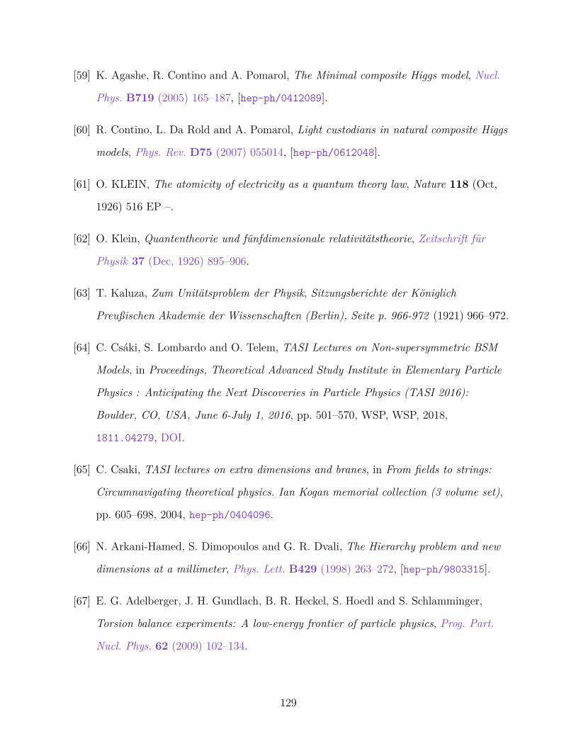
)4 ∼ (200MeV)4 . (1.64)
27
0.01 100.00 106
1010
1014
1018
10-10
1010
1030
1050
1070
Figure 1.1: The evolution of the radiation pressure pR and the vacuum energy density ρV .From left to right, the jumps in the vacuum energy density represent the electroweak, QCDand (hypothetical) GUT phase transitions. Adapted from [45].
Thus, the universe somehow knows when the next phase transition will be [45]. This behavior
is shown in Figure 1.1. This strange property makes the cosmological constant problem one
of most important questions in fundamental physics.
1.5 Organization of the Dissertation
In this dissertation, our aim is to describe two possible approaches for understanding the
problems related to the UV sensitivity of the relevant operators. One approach will be from a
model building perspective while the other one will be from a phenomenological perspective.
We will try to address the hierarchy problem with the former, and the cosmological constant
problem with the later.
In Chapter 2, we will explain most popular proposals for solving the hierarchy problem.
In particular, we will describe models with warped extra dimensions and the AdS/CFT
correspondance in detail, which are the fundamental building blocks of the model we will
present in Chapter 3.
28
In Chapter 3, we will present an attempt for solving the hierarchy problem where we
will try to relate the critical point of the Higgs sector to a minimum in the potential for a
dynamical field. The hope of this relation is to make the Higgs criticality an attractor, so
that a (classical) zero Higgs mass can be obtained for a sizable region in parameter space. We
will build our model on a five dimensional geometry, where the extra dimension is a circle.
The modulus field whose minimum sets the classical Higgs mass to zero will be identified
with the radion, which corresponds to the size of the warped extra dimension. Using the
AdS/CFT correspondance, we will comment on the interpretation of our model as a strongly
coupled approximate conformal field theory in four spacetime dimensions.
In Chapter 4, we will argue that the behavior of the vacuum energy during phase transi-
tions can be tested experimentally using the gravitational waves emitted by a merger of two
neutron stars. Instead of a phase transition at large temperature, we will focus on a phase
transition of QCD which is expected to occur at zero temperature but at very high nuclear
density. Such densities are expected to be found at the cores of heavy neutron stars. If
such a phase transition exists, then it will drammatically affect the equation of state (EoS)
of neutron stars, and such an affect might have a big imprint on gravitational wave observ-
ables. Thus, neutron star mergers might provide an unique test bed for testing whether the
vacuum energy really jumps during the phase transitions.
29
Chapter 2
Solutions to the Hierarchy Problem
In Section 1.2 we have argued that the SM should be treated as an effective theory, and in
Section 1.3 we have shown that this treatment makes the Higgs mass extremely sensitive to
the UV physics and causes the hierarchy problem. In this chapter we will briefly mention
some strategies for taming this problem. Since we have also showed explicitly that the
quadratic divergences are really placeholders for new physics, we take the result in (1.34) as
our starting point.
2.1 Supersymmetry (SUSY)
The main property of SUSY which provides a solution to the hierarchy problem is that
it imposes a relation between the elementary scalars and the fermions, so that the chiral
symmetry which is protecting the fermion masses can be extended to protect the elementary
scalar masses. The SUSY provides exactly this kind of relation.
The mathematical motivation of SUSY comes from the Coleman - Mandula theorem,
which states that it is not possible to build a consistent QFT based on a non-trivial, i.e. non-
commuting, combination of internal symmetries and spacetime symmetries [46]. However,
as shown by Haag, opuszaski and Sohnius, there is one possible exception which is to use a
graded Lie algebra whose generators are fermionic [47].
30
The anticommutation relation which defines SUSY is given by1
Qα, Q
†α
= 2σµ
ααPµ (2.1)
where Q and Q† are SUSY generators, also called supercharges, and Pµ is the momentum
operator. The α, α = 1, 2 are the spinor indices2 and
σµαα =
12×2, σ
i
, σµαα =12×2,−σi
, (2.2)
with σi being the Pauli matrices and 12×2 is the 2×2 unit matrix. Single particle states are
irreducible representations of the SUSY algebra (2.1) and are called supermultiplets. Each
supermultiplet contains an equal number of bosonic and fermionic degrees of freedom [48].
The bosons and the fermions inside the same supermultiplet are called superpartners of each
other. The simplest examples of supermultiplets are
• Chiral supermultiplet: Contains a complex scalar and a Weyl fermion.
• Vector supermultiplet: Contains a gauge field and a Weyl fermion.
The simplest way to make the SM supersymmetric is to assume that each SM degree of
freedom is either in a chiral or in a vector supermultiplet, and introduce superpartners for
them. This is known as the Minimal Supersymmetric Standard Model (MSSM) [49–52]. The
superpartners of the SM fermions are named with a “s-” prefix, while the superpartners of
SM bosons are named with a “-ino” postfix. For example the superpartner of the electron is
called selectron, while the superpartner of the Higgs is called Higgsino. The particle content
of the MSSM is shown in Table 2.1. Notice that there are two Higgs supermultiplets, one
corresponding to the SM Higgs and another with the same SM representations but with
opposite hypercharge. The reason for introducing an extra supermultiplet is to cancel the1This relation can be extended to multiple supercharges QANA=1. In order to solve the hierarchy problem
N = 1 will be enough.2In calculations with spinors, the spinor indices of conjugate spinors, like Q† are written as α.
31
Superpartners SM Particles SU(3)C SU(2)L U(1)YGa8a=1
Ga8a=1
Ad 1 0W a4a=1
W a4a=1
1 Ad 0Li3i=1
Li3i=1
1 −12
eiR3i=1
eiR3i=1
1 1 −1Qi3i=1
Qi3i=1
16
uiR3i=1
uiR3i=1
1 23
diR3i=1
diR3i=1
1 −13
Hu =H+
u , H0u
Hu =
H+
u , H0u
1 1
2
Hd =H0
d , H−d
Hd =
H0
d , H−d
1 −1
2
Table 2.1: Particle content of the MSSM. The description of the representations is the samein Table 1.1. Superpartners are shown with a . A second Higgs supermultiplet is needed tocancel the gauge anomaly.
gauge anomalies.
The degeneracy between fermions and bosons is the mechanism in SUSY which protects
the Higgs mass getting quadratically divergent corrections. As an example, the Λ2 con-
tribution from the top quark loops will be cancelled by the Λ2 contribution from the stop
loops, where stop is the superpartner of the top quark. Of course this requires that both
Yukawa couplings yt be the same but since both top quark and stop live under the same
supermultiplet, this is satisfied by definition in MSSM. Such cancellations occur for all the
diagrams contributing to the Higgs mass to all orders in perturbation theory. An easy way to
see this is to remember that SUSY introduces a degeneracy between the fermion and boson
masses and as we saw at the end of Section 1.3, the fermion masses are protected by chiral
symmetry.
If SUSY were a perfect symmetry of the nature, then the superpartners should have the
32
same masses as their SM partners, and therefore we would have discovered them long time
ago. Since this is not the case, SUSY must be broken at some scale mSUSY. Then following
the discussion of Section 1.4, just by dimensional analysis, we can argue that the quantum
corrections to the Higgs mass in a broken SUSY should have the form
δm2H ∼ λ2
16π2m2
SUSY log
(ΛSUSY
mSUSY
), (2.3)
where λ is some dimensionless coupling and ΛSUSY is cutoff of SUSY. Since the SUSY break-
ing results in mass splittings between the SM particles and their superpartners, mSUSY
determines the order of these splittings. Then (2.2) tells us that irrespective of the cutoff
ΛSUSY, we need mSUSY ∼ O(TeV) in order to get rid of the fine tuning. This condition
is under tense pressure from the results of the LHC experiments [53]. Even if SUSY does
exist in nature, it might not be a perfect solution for the hierarchy problem as people have
thought in the beginning.
2.2 Composite Higgs Models
The main idea behind the Composite Higgs (CH) models [54] is to abandon the idea that the
Higgs is an elementary scalar, and consider it to be a bound state of a strongly interacting
sector. This idea is reminiscent of what happens in QCD, where spin-0 pions are bound states
which arise due to condensation of quarks. Before the discovery of the Higgs, a popular way
to explain the hierarchy problem was using the technicolor models where the electroweak
symmetry breaking occurs directly via a strong condensate, not due to the Higgs [55–57].
Hence technicolor models generally do not predict a Higgs particle, after the discovery of
the SM-like Higgs, such models are strongly disfavored. CH models are modifications of
technicolor models, which produces the Higgs as a bound state3.
The main ingredient of CH models is a new strongly interacting composite sector which3This discussion of CH models is based on [25]
33
confines around the energy scale f ∼ O(1 – 10TeV). This sector emerges from an even more
fundamental theory which is defined at a very high scale ΛUV f . The value of this scale is
not important since the main goal of this construction is to make the Higgs mass insensitive
to higher scales. One further assumes that at the scale ΛUV, this sector sits close to a fixed
point of its RG evolution and there is no strongly relevant deformations around this fixed
point. The motivation behind this assumption is to generate a reasonable hierarchy between
the scales f and ΛUV without introducing severe tuning.
However, this is not enough. If the Higgs were a regular bound state, then its mass
would be comparable to the breaking scale f . Then the composite sector would have con-
fined around f ∼ O(100GeV) and this would have introduced a zoo of bound states, called
resonances, with masses below TeV. Since these states have not been observed, the CH mod-
els should be accompanied by some mechanism which explains the mass hierarchy between
the Higgs and the resonances. This is possible if the Higgs is promoted to a Nambu-Goldstone
Boson (NGB).
NGBs arise due to spontaneous breaking of global symmetries as a result of the Goldstone
Theorem [58]. This theorem states that spontaneous breaking of a global symmetry G into
one of its subgroups H ⊂ G implies the existence of massless degrees of freedom in the
broken theory which are called NGBs. The number of NGBs is equal to the number broken
generators. Mathematically speaking, the NGBs span the coset space G/H. After the
symmetry breaking, the broken part of the global symmetry realizes itself as shift symmetries
for the NGBs. These shift symmetries allow only derivative interactions for the NGBs, hence
quantum correction cannot generate a potential for them. This restriction can be avoided if
the global symmetry G were an approximate symmetry which is explicitly broken by some
terms in the Lagrangian. Then quantum corrections generate a potential for the NGBs,
turning them into pseudo NGBs (pNGBs).
Having all these information, the recipe to create a viable CH model is as follows: First
we have the SM Lagrangian, but without the Higgs potential and the Yukawa interactions.
34
Then we have a strongly interacting composite sector with a global symmetry G which
should at least contain the SU(2)L × U(1)Y subgroup. The explicit breaking of this global
symmetry is done by coupling the global SU(2)L×U(1)Y conserved current of the composite
sector to the electroweak gauge bosons W a. This process is often described as gauging the
SU(2)L × U(1)Y subgroup of G.
An obvious question to ask is what is the minimal possible coset G/H for a viable CH
model. We have said that it should at least contain SUL(2)×U(1)Y . But this is usually not
enough. The strongest constraints to the BSM models come from the electroweak precision
observables, i.e. S and T parameters. The T parameter is more constraining and it predicts
ρ ≡ m2W
m2Z cos2 θW
= 1±O(1%). (2.4)
The reason that this value is very close to 1 is the approximate custodial symmetry in the
SM. To see this symmetry, note that the SM Higgs potential (1.5) is invariant under a global
SU(2)L × SU(2)R symmetry under which
H → ULHU†R, (2.5)
where UL ∈ SU(2)L and UR ∈ SU(2)R. When the Higgs gets a VEV, only SU(2)L part
is broken. There is still a left-over SU(2)R symmetry, known as the custodial symmetry.
Although this symmetry is broken by Yukawa couplings, their contributions to (2.4) are
smaller than 1%.
Therefore a good strategy for model building various BSM models is to respect this
custodial symmetry. With this condition the minimal coset is SO(5)/SO(4). Such a model is
studied in [59,60], where the global symmetry of the composite sector G = SU(3)c⊗SO(5)⊗
U(1)B−L is spontaneously broken into H = SU(3)c⊗SO(4)⊗U(1)B−L4. This model is known
4The U(1)B and U(1)L are symmetries of the SM which correspond to baryon number and lepton numberconservation respectively. While both symmetries are anomalous, their combination U(1)B−L is exact.
35
as the Minimal Composite Higgs Model (MCHM).
2.3 Large/Warped Extra Dimensions
The idea of introducing extra space dimensions in order to solve physical problems dates
back to the attempts by Theodor Kaluza and Oskar Klein to unify gravitation and classical
electromagnetism. Their idea was to introduce a fifth space dimension which is compactified
into a circle of microscopic size [61–63]. This way both the metric of gravitation gµν and the
vector potential of electromagnetism Aµ can be expressed in terms of a 5-dimensional metric
g5mn, which is given by
g5mn =
gµν Aµ
Aµ φr
, (2.6)
where φr is an extra scalar field which corresponds to the 55-component of the 5-dimensional
metric. It is often called the radion.
Although this strategy didn’t accomplish the unification of the gravity and the electro-
magnetism, most of the ideas and terminology in modern extra dimensional theories stem
from the model of Kaluza and Klein. We shall now describe the basics of these models and
explain why there are viable models to address the hierarchy problem5.
The easiest example of an extra-dimensional model is to consider all the extra dimensions
to be flat and are compactified into a circle. Let d denote the dimension of the full spacetime
and D = d− 4 be the number of compactified dimensions. The line element is6
ds2 = gmn dxm dxn , m, n = 0, 1, 2, 3, 5 (2.7)
5We mainly follow [64] in this section.6We will use Roman letters m,n to denote the full d-dimensional spacetime indices, while reserving Greek
letters µ, ν for the usual 4-dimensional spacetime indices.
36
where for flat extra dimensions the metric is
gmn = diag(1,−1,−1, . . . ,−1). (2.8)
Since all the physics we have observed so far are consistent with a four-dimensional spacetime,
we assume that the extra dimensions are compactified into a D-dimensional torus expressed
as
TD =D+4∏i=5
S1(Ri), (2.9)
where S1(R) is a circle with radius R, i.e. R5 and R6 are the radii of fifth and sixth dimensions
respectively.
Now consider a massive real scalar field φ living on a 5-dimensional spacetime. Let us
also denote the 4d spacetime coordinates by x and extra dimensional spacetime coordinate
by y. Then action can be written as
S =
∫d4x dy
(1
2∂mφ(x, y)∂
mφ(x, y)− 1
2m2
0φ(x, y)2
). (2.10)
Since we are interested in the effects of extra dimensions on the four-dimensional physics,
we should find a way to construct a 4d EFT out of this extra dimensional action. This can
be done using a procedure called Kaluza-Klein (KK) decomposition. Here one solves the
equation of motion (EOM) for φ, plug back in the action (2.10) and finally integrate over the
extra dimension. This is also described as integrating out the extra dimension. The EOM
for φ is
(∂m∂
m +m20
)φ(x, y) =
(∂2x +m2
0 − ∂2y)φ(x, y) = 0, (2.11)
where ∂2x ≡ ∂µ∂µ. The key step in the KK decomposition is to use the fact that the extra
37
dimensions are compactified, in order to express the scalar field φ(x, y) as a Fourier series.
If the extra dimension is compactified on a circle of radius R, then the Fourier expansion of
the scalar field becomes
φ(x, y) =1√2πR
∑n∈Z
φ(n)(x) expin
Ry, (2.12)
where Z is the set of integers. Since φ is real, this sets φ∗(n)(x) = φ(−n)(x). Plugging this back
into the action (2.10), integrating out the extra dimension using the orthogonality relations
gives
Seff =
∫d4x
(∂µφ
∗(0)∂
µφ(0) −m20
∣∣φ(0)
∣∣2)+ ∞∑n=1
(∂µφ
∗(n)∂
µφ(n) −n2
R2
∣∣φ(n)
∣∣2) . (2.13)
So in the effective theory we have a complex scalar field φ(0) with the mass m0 plus an
infinite number of heavy particles with masses mn = n/R, which are called KK modes, or
KK tower. As the radius of the extra dimension is getting smaller, the masses of KK modes
become heavier.
A similar analysis can also be done for the gauge fields for which the action reads
S =
∫d4x dy
(−1
4FmnF
mn
), (2.14)
where Fmn = ∂mAn − ∂nAm, and
Am =
Aµ
A5
. (2.15)
Under 4d-Poincare transformationsAµ is a vector whileA5 is a scalar. The KK decomposition
38
can be done as in the scalar case. The Fourier expansion is
Am(x, y) =1√2πR
∑l∈Z
A(l)m (x) exp
il
Ry
. (2.16)
Plugging this into (2.14) and performing the integration over the extra dimension gives
Seff =
∫d4x
[−1
4F (0)µν F
µν(0) +1
2∂µA
(0)5 ∂µA
(0)5
]
+∞∑l=1
[−1
2F (l)µνF
µν(−l) +l2
R2A(l)
µ Aµ(−l) − i
l
R
(A(l)
µ ∂µA
(−l)5 − Aµ(−l)∂µA
(l)5
)].
(2.17)
The last term suggest a mixing between A(l)µ and A
(l)5 when l 6= 0. But this mixing can be
removed by gauge freedom. Namely in the 5d axial gauge we can set
A(l)µ → A(l)
µ − i
l/R∂µA
(l)5 , A
(l)5 → 0, for l 6= 0, (2.18)
which removes this mixing term. So the effective action we get is
Seff =
∫d4x
[−1
4F (0)µν F
µν(0) +1
2∂µA
(0)5 ∂µA
(0)5
]+ 2
∞∑l=1
[−1
4F (l)µνF
µν(−l) +1
2
l2
R2A(l)
µ Aµ(−l)
].
(2.19)
So in the effective theory we have a massless gauge boson F(0)µν , a massless scalar field A
(0)5
and a tower of massive gauge bosonsA
(l)µ
∞
l=1. The excitations of A5’s are unphysical since
they can be removed by gauge fixing.
Now consider the gauge covariant derivative in this setup. It is given by
Dm = ∂m − ig5Am, (2.20)
where g5 is the 5d gauge coupling. Since [∂m] = 1, from (2.14) the mass dimensions of the
39
field strength Fmn and the gauge field Am should be [Fmn] = 5/2 and [Am] = 3/2 in 5d. But
then (2.20) tells us that the 5d gauge coupling g5 should be dimensionful and [g5] = −1/2.
We can get a dimensionless effective 4d gauge coupling by plugging the Fourier expansion
(2.16) into (2.20). This way we find
Dµ = ∂µ − ig5
(1√2πR
A(0)µ + . . .
), (2.21)
which says that the effective 4d coupling constant g4 is
g4 =g5√2πR
. (2.22)
This result can be generalized to higher dimensions by [65]
g24 =g24+D
volD, (2.23)
where volD is the total volume of the extra dimensions.
Same exercise can also be done for the gravitational coupling. The Einstein-Hilbert action
in a flat spacetime with D extra dimensions is given by7
S4+D = −M2+D4+D
∫d4+Dx
√|g4+D|R4+D, (2.24)
where M4+D is the analog of Planck scale in higher dimensions. For flat extra dimensions
we have R4+D = R4 at linear order [65], thus after integrating out the extra dimension we
get
S4+D = −M2+D4+D
∫dDx
√|gD|
∫d4x
√|g4|R4 = −M2+D
4+D volD
∫d4x
√|g4|R4, (2.25)
7The power of the Planck scale 2 +D comes from the fact that the mass dimension of the Ricci scalar is[R] = 2 in all dimensions.
40
Thus we obtain the Planck scale in an extra dimensional theory as
M2+D4+D =
M2pl
volD. (2.26)
We can now try to estimate the natural size of the extra dimension. The simplest as-
sumption would be that all dimensionful parameters are set by the same physical scale and
take that scale to be M4+D. By generalizing the exercise following (2.20), we can find that
in the case D extra dimensions [g4+D] = −D/2, so the natural size of this gauge coupling is
g4+D ∼ 1
MD/24+D
. (2.27)
Combining this result with (2.26) and (2.23) gives
vol1/D ∼ R ∼ 1
Mplg− 2+D
D4 , (2.28)
where R is the average size of the extra dimensions. The result shows that the natural size
of the extra dimensions would be on the order of the Planck length lpl ∼ 10−35m and the
KK modes are at the Planck scale. Clearly this is not a viable phenomenological model.
Moreover this model didn’t help to solve the hierarchy problem at all. It is important to
keep in mind that in this setup all the SM particles are propagating in the bulk, which is the
space spanned by the extra dimensions. We shall see now the situation drastically changes
if one relaxes this assumption.
Instead of letting them to propagate through the whole bulk, the fields can be localized
by introducing the concept of branes. Branes are 3 + 1 dimensional hypersurfaces with
localized stress-energy tensor so that fields can be trapped on them. Mathematically one
can define them as topological defects of some sort. String theories have similar objects,
called D-branes where open strings are attached. From a BSM model building point of view,
it is not important how these branes did end up there. All the models we will mention in
41
this section should be considered as effective field theories valid up to some cutoff scale ΛUV.
Proper explanation of the branes should be handled by some new physics which is expected
to replace the effective description at the cutoff scale.
The simplest implementation of branes in extra-dimensional theories is the scenario of
Large Extra Dimensions, introduced by Arkani-Hamed, Dimopoulos, and Dvali [66]. In their
model, all the SM fields are localized on a brane, and only gravity can propagate through
the bulk. Then, as a consequence of (2.26) one can lower the fundamental scale of gravity
M4+D ≡M∗ considerably by choosing volume the extra dimensional space volD to be large.
Since M∗ is the cutoff which will enter to the SM calculations, lowering M∗ to the TeV would
solve the hierarchy problem.
If there are D extra dimensions with a similar radii R, then from (2.26) we can write
R ∼ 1
M∗
(Mpl
M∗
)2/D
. (2.29)
Choosing M∗ ∼ 1TeV and Mpl ∼ 1019GeV gives
R ∼ (1TeV)−1 × 1032/D ∼ 10(32/D−19)m. (2.30)
For d = 1, this gives R ∼ 1013m which is on the order of the solar system and is clearly ruled
out. For d = 2, we get R ∼ 1mm. Although this might seem large too, it is very hard to
experimentally test the gravity. The current bound isR < 37 µm [67,68] which excludes d = 2
with M∗ ∼ 1TeV, but not too much. This bound can be avoided if M∗ & 3TeV. However
much stringent bounds exist from astrophysical and cosmological observations which pushes
M∗ to M∗ > 10 – 103TeV [69–71].
For larger D, the sizes of extra dimensions are within experimental limits. However this
idea has one big conceptual issue. If M∗ is the fundamental scale of the theory, then the
size of the extra dimension should also be determined by that scale, which would imply
R ∼M−1∗ . But (2.29) shows that if there is a large hierarchy between Mpl and M∗, which is
42
needed to solve the hierarchy problem, then R M−1∗ . In other words, this model redefines
the hierarchy problem between the weak scale and gravity to the hierarchy problem between
the size of the extra dimension and the fundamental gravity scale.
An obvious next step would be to abandon the assumption flat extra dimensions and
consider extra dimensions with non-trivial geometry. This is not an easy task though since
it is generally very hard to find gravity solutions. Such a solution were found by Randall
and Sundrum in their famous paper [72]. They showed that a metric of the form
ds2 =
(R
z
)2 (ηµν dx
µ dxν − dz2). (2.31)
with R being a constant, is a solution to the 5d Einstein equations on a 5d interval with
negative cosmological constant Λ, bounded by two branes having tensions T0 and T1. These
branes are called UV and IR branes respectively. (2.31) is the metric for the 5-dimensional
Anti-de-Sitter AdS5 space and the conformal factor (R/z)2 is called the warp factor. We will
see that this warp factor will play a big role in addressing the hierarchy problem. This model
and other models which are based on this one are called Randall-Sundrum (RS) models in
the literature.
We will now calculate the effective 4d gravity and gauge couplings. We will assume that
the branes are located at z0 ∼ R ∼M−1pl and z1 ∼ R′ ∼ TeV. Matching the gravity coupling
is slightly more involved in this case, since the extra dimension is not flat. This can be done
by embedding the 4d graviton hµν(x) into the AdS5 metric as [65]
ds2 =
(R
z
)2 [(ηµν + hµν(x)) dx
µ dxν − dz2]. (2.32)
What we need to calculate is how the Ricci tensor R(4)µν calculated from hµν is contained in
R(5)µν which is calculated from (2.32). Since both metrics differ only by a conformal factor
43
(R/z)2 we find
R(5) ⊃(R
z
)2
R(4). (2.33)
Then the effective gravity action becomes
Seff = −M3∗
∫d4x dz
√|g(5)|R(5) ⊃ −M3
∗
∫ R′
R
dz
(R
z
)3 ∫d4x
√|g(4)|R(4). (2.34)
By performing the integral over the extra dimension, we find the effective Planck scale as8
M2pl =M3
∗R
[1−
(R
R′
)2]. (2.35)
We see that for R ∼ M−1∗ , we have Mpl ∼ M∗ so unlike in the large extra dimensional
scenario, in warped space models there is no hierarchy between the 4d and the 5d gravity.
Let us do a similar exercise for the weak scale. For simplicity, assume that there is only
the Higgs field and is localized on the TeV brane. Then we can add the following term to
the 5d action:
S(5) ⊃∫
d4x dz√−g1δ(z −R′)LH , (2.36)
where g1 is the induced metric on the TeV brane, (g1)µν = (R/R′)2ηµν , and LH is the usual
Higgs Lagrangian:
LH =(∂µH†) (∂µH) +m2
H |H|2 − λH |H|4. (2.37)
8There is an extra factor of 2 in this result coming from the fact that in RS models one usually considersthe extra dimension to be a S1/Z2 orbifold. In these configurations the extra dimension starts as a circleS1 with a radius rc and domain −πrc ≤ y ≤ πrc. The branes located at y0 = 0 and y1 = πrc. Then oneimposes a Z2 symmetry by y → −y so that the theory is formulated on a line segment 0 ≤ y ≤ πrc. Howeverthe integration over the extra dimension contains a double copy of this line, and hence we get an additionalfactor of 2.
44
The crucial part is that we have to use the induced metric to raise and lower the Lorentz
indices in this expression, i.e.
(∂µH†) (∂µH) = gµν1
(∂µH
†) (∂νH) =
(R
R′
)−2
ηµν(∂µH
†) (∂νH) . (2.38)
Now we can integrate out the extra dimension to get an effective 4d action
S(4) ⊃∫
d4xL(4)H , (2.39)
where
L(4)H =
(R
R′
)2
ηµν(∂µH
†) (∂νH) +
(R
R′
)4
m2H |H|2 − λH
(R
R′
)4
|H|4. (2.40)
However the Higgs kinetic term is not canonically normalized. We can normalize it by
rescaling the Higgs by H → (R′/R)H. After this rescaling we obtain
L(4)H = ηµν
(∂µH
†) (∂νH) +
(R
R′
)2
m2H |H|2 − λH |H|4. (2.41)
The scaling factor in front of the Higgs mass term is the key property of RS models which
makes them a popular solution to the hierarchy problem. We can see that even mH is set by
M∗, which would naturally be the case, in the 4d effective theory it appears much smaller
provided that R/R′ 1. In particular, for M∗ ∼ 1019GeV and mH ∼ 102GeV, one needs
R/R′ ∼ 10−17. This result shows the key distinction between the large and the warped extra
dimensions. In large extra dimensions, both weak and gravity scales are at TeV, but the
apparent gravity scale is Mpl due to its dilution through the extra dimension. On the other
hand in RS models, both weak and gravity scales are at Mpl, but the weak scale warped
down by the extra dimension so its apparent 4d scale is TeV.
Now the question is how can we get a hierarchy of R′/R ∼ 1017 naturally? In RS model,
45
this needs to be set by hand since there is no mechanism which can stabilize the size of the
extra dimension. A stabilizing mechanism was found by Goldberger and Wise shortly after
the RS paper, and it is usually called Goldberger-Wise (GW) mechanism in the literature [73].
GW did consider a massive scalar field Φ living the bulk whose action is
SGW =1
2
∫d4x dz
√g(gmn∂mΦ∂nΦ−m2Φ2
). (2.42)
Again there are UV and IR branes, but this time they contain potentials for Φ:
Sbrane = −∑i=0,1
∫d4x
√−giλi
(Φ2 − v2i
)2, (2.43)
where the subscripts 0 and 1 represent parameters for the UV and the IR branes respectively.
These potentials cause the bulk scalar Φ to develop a z-dependent VEV, which can be
obtained by solving the classical EOM arising from the variation of (2.42) with respect to
Φ. The unique solution can be found with the help of the two boundary conditions imposed
by the branes. This solution can then be put back into the action (2.42) and the extra
dimension is integrated out. After all these steps one obtains a 4d effective potential for the
size of the extra dimension. GW then showed that the effective potential has a minimum
around
log
(R′
R
)≈(
2
mR
)2
log
(v0v1
). (2.44)
For log(v0/v1) ∼ O(1), a large hierarchy R′/R ∼ 1017 can be generated by a modest value
of (mR)2 ∼ (m/M∗)2 ∼ 0.1.
In the paper of GW, the form of the metric is held constant, i.e. the backreaction of the
scalar field Φ on the metric is ignored. The coupled scalar-gravity equations can be solved
exactly for some bulk potentials, including the potential used in the GW model, using the
superpotential method [74]. Such a calculation for one scalar field is presented in [75] while
46
the generalization to multiple fields is also possible [76].
2.4 AdS/CFT Correspondence
In this final section of this chapter, we will see how the CH models we have presented in
Section 2.2 and RS models we have presented in Section 2.3 can be related to each other
by using one of the most powerful ideas in theoretical physics in recent years, which is the
gauge-gravity duality. The main reference for this section will be [77].
In physics, duality means the description of a physical system in completely different
ways having entirely different degrees of freedom and interactions. As a basic intuition, one
can think of a system, such as QCD, which is weakly coupled at high energies and therefore
perturbative. At this energies, its degrees of freedoms are approximately free. However at
lower energies this theory becomes strongly coupled, its degrees of freedom are no longer
uncoupled from each other, and therefore perturbation theory breaks down. But at strong
coupling, bound states of fundamental degrees of freedom might be formed and these can
behave as a new set of variables which are weakly coupled to each other. So it is somehow
expecting that a system should be able to described differently at different energies.
The AdS-CFT correspondence [78] is a special example of a general class of dualities
known as gauge-gravity dualities. It is duality between Type IIB string theory on AdS5 × S5
and N = 4 Super-Yang-Mills theory which is a Conformal Field Theory (CFT) in four
dimensions with the gauge group SU(N). The parameters on both sides of the duality are
related to each other by
(R
ls
)4
⇔ 4πg2YMN, (2.45)
where R is the AdS radius, ls is the string scale and gYM is the gauge coupling on the CFT
side. In order to describe gravity on the AdS side classically, one needs R ls which means
on the CFT side we need g2YMN which corresponds to strong coupling. The usefulness of
47
this duality lies in this observation. We can explain strongly coupled field theories by doing
calculations with classical gravity.
The symmetry group of a conformal Poincare-invariant field theory in d dimensions is
the conformal group SO(d, 2). This group contains the Poincare transformations, d special
conformal transformations and a scale transformation given by
D : t→ λt, x → λx. (2.46)
Conformal field theories are field theories which are invariant under this transformations,
hence they lack a physical scale. The main motivation behind the AdS/CFT correspondence
is the fact that the isometry group9 of AdSd+1 is also SO(d, 2). The scale transformations in
(2.45) are reflected on the AdS side as
D : t→ λt, x → λx, z → λz. (2.47)
The last transformation is crucial. It says that a scale transformation on the CFT corre-
sponds to a movement in the extra dimension. Since scale transformation is related to RG
evolution in a field theory we have
movement in extra dimension ⇔ RG evolution in 4d theory.
Breaking one the symmetries on one side corresponds to breaking it on the other side.
The branes we have encountered in Section 2.3 do break the AdS isometry, so they correspond
to breaking of conformal symmetry on the CFT side.
A global symmetry of the field theory is realized as a gauge symmetry on the AdS side.
But there is no such requirement for the gauge symmetries of the field theory. This is
not surprising since gauge symmetries are not real symmetries; they are redundancies in the9An isometry is a map between two metric spaces which preserve the distance.
48
description. Moreover since different gauge symmetries are characteristics of different degrees
of freedom, so it is expected that they don’t match. However gauge invariant quantities are
physical, therefore they should match. This is indeed true. Each field on the gravity side
corresponds to a gauge invariant operator in the field theory.
To see this explicitly, let us consider the action given in (2.42) without any branes but in
d+ 1 dimensions. Close to the boundary of the AdSd+1, z → 0, we can express the solution
to Φ as
Φ(z → 0, x) = z∆−[α(x) +O(z2)
]+ z∆+
[β(x) +O(z2)
], (2.48)
where α(x) and β(x) are functions of the 4D coordinates and
∆± ≡ d
2±√d2
4+m2R2. (2.49)
Since z → λz under a scaling transformation, the functions α and β should scale as
α(x) → λ−∆−α(x) and β(x) → λ−∆+β(x). (2.50)
One of these functions should be fixed by boundary conditions. A commonly used choice is to
fix α by α(x) ≡ J(x) for some choice of J(x). This way β(x) becomes a dynamical variable
which in the field theory can be identified with an operator O(x) with scaling dimension
∆+. Since O(x) is turned on after introducing J(x), J(x) is identified as a source for the
operator O(x). Note that this implies the scaling dimension of J(x)O(x) is ∆+ + ∆− = d
which should be the case for a field theory in d dimensions. In summary, AdS/CFT provides
a relation between the partition functions of the gravity and the field theory:
Z[Φ;α(x) = J(x)] ⇔ ZCFT[source for O(x) is J(x)]. (2.51)
49
Although it is expected that this relation to hold for generic models, we only know how to
do classical gravity. The left hand side of this relation approaches to the classical gravity if
one considers the large-N limit on the CFT side, i.e. when g2YMN 1.
Since the scaling dimension of O is ∆+ using (2.49) we can classify O as
irrelevant if m2R2 > 0,
marginal if m2R2 = 0,
relevant if m2R2 < 0.
(2.52)
Unlike the Minkowski space, the AdSd+1 space allows scalar having negative masses as long
as they satisfy the Breitenlohner-Freedman (BF) bound [79, 80]:
m2R2 ≥ −d2
4. (2.53)
This sets the bound ∆ ≥ d/2 for any operator in the CFT. However this bound can be
lowered to ∆ ≥ d/2− 1 by modifying the gravity action with boundary terms [81].
With all these information we can build the bridge between the Composite Higgs and the
Randall-Sundrum models. We will try to explain the general picture without specifying how
the individual fields are related to each other, since they can be model dependent. We start
with a pure AdS5 space without any branes which is dual to a strongly coupled 4d CFT, and
we identify this CFT with the composite sector of CH models. We will add ingredients one
by one to either side and describe the related deformation on the other side, as it has been
done in [82] which we shall follow closely.
Let us start by adding a UV, or Planck, brane. On the CFT side this gets translated
to an UV cutoff ΛUV, at which the CFT description breaks down. Since the metric is still
pure AdS, we still have an exact CFT below the cutoff. Moving the UV brane from 1/R to
1/R where R > R corresponds to integrating out the degrees of freedom between the energy
scales Λ = 1/R and Λ = 1/R.
50
Putting an IR, or TeV, brane at R′ = 1/Λ′ strongly breaks the conformal invariance of
the composite sector at 1/Λ′. If all the SM fields live on the TeV brane like in the RS model,
then this would imply that all the SM fields emerge as bound states of the composite sector.
So from the 4d point of view, the RS model is a theory where the SM is embedded inside a
strongly coupled CFT above the TeV.
Now add a scalar field to the bulk as in the GW mechanism. We already know that it
should correspond to an operator on the CFT side OΦ with scaling dimension
∆+ = 2±√4 +m2R2 ≈ 4 +
m2R2
4, for small m2R2. (2.54)
We see that for smallm2R2, the operator OΦ is marginally relevant form2 < 0 and marginally
irrelevant for m2 > 0. This operator is sourced by the coefficient of z∆− term of (2.48). All
these amount to perturbing the CFT by an operator
LCFT → LCFT + JOΨ, (2.55)
which mildly breaks the conformal symmetry explicitly. The RG running of this operator
is determined by the RG running of its coupling constant J , which will be Jz∆− . Since
∆− ≈ −m2R2
4, for m2 < 0 this coupling will grow towards the IR and at some point breaks
the CFT, which is realized on the AdS side as the IR brane. The m2 > 0 case can be thought
as a mechanism for generating the UV brane. In this case the coupling will grow towards
the UV and breaks the CFT at some UV scale, which is realized on the AdS side as an UV
brane.
51
Chapter 3
Self-Organized Higgs Criticality
3.1 Introduction
The Higgs instability in the electroweak sector of the Standard Model (SM) appears thus
far to be of the simplest variety, with the Higgs sector residing “unnaturally” close to a
critical point seemingly unprotected by symmetry and well described by mean field theory.
The Higgs sector is associated with a Landau-Ginzburg theory of a symmetry breaking
phase transition. The Higgs field of the Standard Model develops a vacuum expectation
value (VEV) due to a relevant operator (the Higgs mass term) having the “wrong sign”
in the infrared which destabilizes the origin in field space. The naturalness issue, or the
hierarchy problem, is the statement that in units of the much larger fundamental scales in
the problem, i.e. the Planck or GUT scales, the bare mass must be tuned to an absurd degree
to accommodate the observed value for the VEV and the mass of the Higgs particle, and
that quantum corrections spread this sensitivity among fundamental parameters. That is,
quantum effects make the Higgs mass similarly sensitive to, for example, the value of the top
quark Yukawa coupling. As a consequence it is expected that low energy effective theories
with Higgs sectors like that of the SM are extraordinarily rare when there are other large
physical scales present.
52
Most proposed resolutions of this problem invoke new symmetries requiring new particles
with fixed interactions that ameliorate the sensitivity of the Higgs mass to larger mass scales.
The paucity of new particles at the TeV scale has sown growing doubt that this is the way
nature has created a low electroweak scale.
In this work, we begin an investigation of the possibility that the critical point for Higgs
sectors like that of the SM can arise naturally not due to symmetry, but rather because of a
self-organization principle, as suggested in [83]. This is inspired by critical behavior that has
been observed in a wide variety of seemingly unrelated physical systems in nature [84, 85],
with the canonical example being the sandpile. In this example, a pile of sand is created
and sustained by slowly pouring sand from a funnel onto a fixed point. The sand self-
organizes into a cone with opening angle fixed by microscopic interactions between grains.
Perturbations, even if only involving a single grain of sand, result in avalanches at all scales,
following a power law distribution. After the avalanche, when the system has removed the
perturbation, the cone of sand is in a new configuration, but still critical so long as sand
continues to be slowly added. Such “self-tuning” is also thought to arise at earthquake fault
lines, river bifurcations, and temporally near financial market crashes [86]. It has been key
to describing some astrophysical phenomena as well [87]. It has been hypothesized that
these phenomena of criticality at the threshold of “catastrophic failure” can be related to an
instability arising from critical exponents becoming complex, corresponding to discrete scale
invariance [88]. This possibly suggests an approach to the Higgs fine-tuning problem in extra-
dimensional models in AdS space, where similar features appear when the Breitenlohner-
Freedman (BF) bound [80] is violated, leading to complex scaling dimensions and a complete
loss of conformality in a hypothetical 4D dual [89].
Typically, in the examples we have in statistical physics, criticality is “self-organized” by
temporal loading of the system: the slow addition of sand grains at a pile’s apex, gradual
stress building at faults due to tectonic drift, etc. In relativistic theories, this slow temporal
loading can be exchanged with mild spatial gradients, and in 5D, through the AdS/CFT
53
duality [78], spatial translation and gradients can be, in turn, related to scale transforma-
tions and renormalization group evolution. This further suggests an approach where the
instability associated with complex scaling dimensions is reached dynamically through slow
renormalization group evolution, or, in a 5D dual, via growth of a deformation of AdS space
that leads to eventual violation of the BF bound. This has a parallel in some perturbative
4-dimensional theories where dimensional transmutation directs the Higgs potential [90]. In
models such as the MSSM, the instability of the electroweak sector can be arrived at through
quantum corrections [91–93]: RG flow from some microscopic theory seemingly devoid of in-
stabilities evolves to an IR theory where a Higgs picks a non-vanishing condensate.
Stepping away from the background motivation, we can state generally that the eventual
goal of this line of research is to have a zero for the Higgs mass term coinciding (or nearly
coinciding) with a minimum in the potential for an extra-dimensional modulus field over a
wide range of extra-dimensional input parameters. In this case Higgs criticality would be a
dynamical attractor for the theory without extreme sensitivity to fundamental constants. In
other words, such a 5D system self-tunes to the critical point of its 4D low energy effective
Higgs theory. This is similar to the way in which the strong CP problem is resolved by the
axion hypothesis where the axion field promotes the CP phase to a dynamical field whose
potential minimum resides at the point where CP is conserved in QCD, and also to models
which solve the hierarchy problem using cosmological dynamics and slightly broken shift
symmetries [94].
To be properly identified as self-organization, in the most conservative application of
this label, criticality near the minimum of the potential must be robust under reasonable
variation of model input parameters: we are looking for a theory with a near-critical Higgs
region. From the perspective of the low energy theory, at energy scales below the modulus
VEV, the lightness of the Higgs would be in apparent violation of effective field theory
principles and power counting, that is, a violation of the principle of locality of scales.1
1Such violation has been observed before in a toy model with discrete scale invariance [95], anothersuggestive connection to self-organized critical systems.
54
ϕ
V(ϕ)
m2H = 0
m2H > 0 m2
H < 0
Figure 3.1: This figure exhibits a cartoon of a potential for a modulus field, φ, where the singularminimum matches on to a critical point at which the mass of a physical light Higgs field fluctuationpasses through zero. On either side of the singular point, the Higgs boson mass is finite and positive,but on one side the mass squared for the field is negative, with the instability driving spontaneoussymmetry breaking.
This could be reconciled by the fact that in a microscopic 5D theory, quantum corrections
might renormalize the potential for the Higgs and modulus field simultaneously, shifting the
location of the minimum, but not the property that the physical Higgs boson is light at
that minimum. A cartoon is shown in Figure 3.1. We emphasize that this has not yet been
realized in a dynamical model in this work, but rather is a longer term goal in which this
paper could be a crucial first step.
To realize such a scenario, there first must be a feedback mechanism, such that when the
Higgs field develops a VEV, the potential for the modulus responds, as shown in Figure 3.1.
This is somewhat akin to the way thresholds can play an important role in Casimir energies,
as in, for example [96]. If this feedback is itself the origin of the minimum of the potential,
with the minimum being at or near the critical value at which the Higgs VEV turns on, the
modulus field will be attracted to the minimum, where the mass of the Higgs fluctuation is
small or vanishing.
In one “toy” and one fully dynamical construction, we investigate the mutual potential
55
of a modulus field (in our case, the radion of a Randall-Sundrum (RS) 2-brane model [72])
and a 5D Higgs field. The models are constructed so that the value of the modulus field
vacuum expectation value influences the Higgs stability criterion. Specifically, we consider
scenarios where the Higgs instability is linked to dynamical violation of the BF bound far
from the UV boundary of the RS geometry through interactions with the modulus field.
The CFT dual of this picture corresponds to the theory described above: one which is
conformal in the deep UV, without instabilities, and which contains a near marginal defor-
mation that drives a slow running of the scaling dimension of an operator in this approximate
CFT [82, 97]. There is an interplay between two operators, Oε, a near marginal operator,
and OH . Similar to the way dynamical symmetry breaking for the Higgs can occur via
radiative corrections, here an analogous instability is reached in the RG flow for the dual
picture, with the scaling dimension for the operator OH becoming complex, and causing an
“unhealthy” [98] limit cycle-like behavior in the RG flow that is terminated by condensa-
tion of operators in the approximate CFT, breaking the approximate conformal invariance
spontaneously.
Curiously, in the models studied here, a nontrivial cosmology may be a common feature
of the classical ground state. In the 5D picture, the metric and scalar fields must include
a cosmology for the low energy 4D effective theory in order to satisfy the metric junction
conditions for the two brane model, unless UV and IR brane tensions are tuned. We sus-
pect this is due to a frustration mechanism similar to that which causes striped and other
inhomogeneous phases to appear in some high Tc superconductors [99], and may lead in this
case to a time-dependent vacuum state [100, 101]. Studies of holographic superconductivity
have identified such phases when the BF bound is violated deep in the interior of asymp-
totically AdS geometries due to non-trivial gauge and gravitational field backgrounds [102].
In other words, the resolution of the RG limit cycle instability may have its imprint in the
low energy theory as a limit cycle in time evolution. We have left a full exploration of the
time dependence for future work, however we do speculate on the possible relevance of this
56
feature for cosmology [103,104].
The chapter is organized as follows: In Section 3.2, we set the stage with a discussion of
a possible effective theory for a dilaton vacuum expectation value that has features that we
find in our holographic model, and which points towards a new way to set the confinement
scale in an approximately conformal theory. In Section 3.3, we describe a 5D toy holographic
implementation of these ideas that leaves out certain backreaction terms, with a bulk Higgs
mass that is given explicit dependence on the extra-dimensional coordinate. In Section 3.4,
we show how to promote this simplest model to a dynamical one, where the effective Higgs
mass evolves due to a coupling to a “driving” scalar which picks a coordinate-dependent
VEV. In Section 3.5 we discuss in more detail a possible approximate CFT interpretation
of the 5D model, and make some connections to generalized BKT scaling discussed in [89].
In Section 3.6, we briefly discuss connections to self-organized critical models in statisti-
cal physics, to catastrophic failure modes of these systems, and future implementation of
these ideas into an extension of the SM. Finally, we discuss aspects of the cosmology of the
model, part of which involve speculation that can be more fully resolved with future work,
in Section 3.7.
3.2 Preliminaries: The Frustrated Dilaton
We begin by considering an effective theory of a dilaton that has aspects of the behavior of the
more detailed holographic models we consider. In an approximately scale-invariant theory
that undergoes spontaneous breaking, the potential that sets the scale of that breaking is
a (nearly) scale-invariant quartic: Vdil = α(f)f 4, where α has some weak dependence on f
that encodes the amount of explicit breaking. This potential can have a nontrivial minimum
at small values of f if α obeys some basic properties.
It is important to note that in this effective theory, f is a summed total scale of conformal
breaking, and relations between individual VEVs are hidden in this potential. In other
57
words, many operators could be simultaneously condensing which all contribute to conformal
breaking. In addition, if there is some small breaking of conformal invariance, there can be
nontrivial relations between these operator VEVs that are not encoded in the total dilaton
potential.
Now we note that it could be the case that there is simply no solution that satisfies
the relation between VEVs in the approximate CFT for a total f below some critical value,
f < fcrit. How does the theory exit the CFT in this case? The dilaton is frustrated –
internally, it seeks to satisfy the relations between operator VEVs, providing a lower limit to
the total breaking scale. On the other hand, in the low energy theory, a smaller or vanishing
f is preferred.
As a very simple example of this, we could consider two VEVs fφ and fhiggs where at
some critical value of decreasing fφ, fhiggs begins to turn on:
f 2higgs =
−λfφ−µ2
λHλfφ − µ2 < 0
0 otherwise.
Such behavior occurs in the “relaxion” models of electroweak symmetry breaking. Note
however, that we are not specifying a global potential for this behavior, but instead are
merely providing an ad hoc relationship between operator VEVs that might arise inside of
the approximate CFT. In the holographic models we consider, fφ corresponds to the VEV of
a marginally relevant operator, and fhiggs to the VEV of an operator whose scaling dimension
is driven into the complex plane.
If these VEVs contribute to an effective dilaton potential as Vdil ≈ α(f 4φ + f 4
higgs) (as
though they are both from operators with scaling dimension near 4), the potential will be
globally minimized when f 2φ = λ
2λHfφf 2
higgs if the relationship between VEVs is maintained.
A large hierarchy between fhiggs and fφ can be created by having a small value of λH , and
the dilaton potential appears to be minimized at some fcrit while enforcing the relation.
We note that the dilaton potential itself does not enforce the relation between the VEVs,
58
which is instead specified by some dynamics that is part of the UV completion of the dilaton
effective theory. This can create a puzzle from the perspective of the low energy theorist,
which sees only the total breaking scale f , not the interrelations between the individual
f ’s that contribute. The low energy observer would think that f = 0 should minimize the
pure quartic potential, but instead the theory gets “trapped” at a larger f . Of course these
relations between VEVs would require some breaking of scale invariance, and the potential
would not be precisely quartics.
There may be a connection here to the concept of frustrated phase separation in con-
densed matter physics, a phenomenon where (for example) high Tc superconductivity is
blocked due to long range Coulomb interactions, and the theory resolves the tension by
creating an intermediate phase which spontaneously breaks translation invariance, creating
“stripes” [99]. Here, Higgs condensation may be blocked by quasi-long range dilaton inter-
actions, and there may be some analog of these striped phases that resolves the frustration
that is important for cosmology.
With this hypothetical scenario as context and motivation, we begin our holographic
studies.
3.3 Toy Model: Explicitly Varying Higgs Mass
To illustrate a basic model with the features we seek, we work in 5D asymptotically anti-de
Sitter space without a UV brane, and give the Higgs a bulk mass term that varies explicitly
with the extra-dimensional coordinate. We strongly emphasize that this is a toy model
that easily illustrates some curious features that help motivate the more realistic model in
Section 3.4. Specifically, this model leaves out backreaction between the Higgs and the (here
unspecified) dynamics that give rise to the varying mass term, while in Section 3.4, this
backreaction is taken fully into account.
The metric can be written as (setting the AdS curvature near the AdS boundary, k, to
59
1) [105]:
ds2 =1
z2
[dx24 −
dz2
G(z)
]. (3.1)
The coordinate z ranges from 0 at the AdS boundary to an IR brane at z = z1, and for
z → 0, the function G has the asymptotic behavior G(z) → 1 and G′(z) → 0. Away from
z = 0, the function G encodes the effects of gravitational backreaction due to nontrivial bulk
physics such as condensates. We are restricting our ansatz for the background to solutions
obeying 4D Lorentz invariance.
The action is given by
S =
∫d4xdz
√g
[|∂MH|2 + 6
κ2−m2(z)|H|2 − 1
2κ2R
]−∫d4xz−4m2
0|H|2∣∣∣∣z→0
−∫d4xz−4V1(|H|)
∣∣∣∣z→z1
,
(3.2)
with κ2 = 1/(2M3Pl). The bulk mass function is chosen to a have fixed value in the limit
z → 0, and decreases monotonically and slowly as z increases:2
m2(z) = −4 + δm2 − λzε. (3.3)
Note that m2 = −4 corresponds to the Breitenlohner-Freedman bound, and δm2 is taken
to be a positive quantity so that the z → 0 limit is well-defined.3 We note that past work
explored constant Higgs bulk mass at or near the BF bound [106, 107] with interesting
implications for radius stabilization. A possible relationship between the BF bound and
scalars with suppressed mass in lattice studies of theories at the boundary of the conformal2It is not difficult to arrange for this type of z-dependent mass term to arise dynamically, rather than
through this forced explicit breaking of the isometries of AdS. We give examples in Section 3.4.3If the mass is taken below the BF bound as z → 0, perturbations solving the scalar equation of motion
oscillate rapidly in the UV, indicating the need for an ultraviolet cutoff, such as a brane that cuts off thesmall z region of the spacetime [89].
60
window was discussed in [108]. For the IR brane potential, we take
V1(|H|) = T1 + λH |H|2(|H|2 − v2H
), (3.4)
where T1 is the tension of the brane. The Higgs may, for some regions of parameter space,
pick a nonvanishing vacuum expectation value, 〈H〉 = φ(z)/√2, where the Higgs VEV has
a nontrivial profile along the z-coordinate.
Restricting to solutions that obey 4D Lorentz invariance, the 5-5 component of the Ein-
stein equations relate the metric function G to the behavior of the Higgs VEV in the bulk:
G =−κ
2
6V (φ)
1− κ2
12(zφ′)2
, (3.5)
and they can be further employed to reduce the effective potential for the classical background
configuration to a pure IR boundary term [75]:
Vrad =1
z41
[V1(φ) +
6
κ2
√G
]. (3.6)
There is generally a UV contribution from the brane at z0 as well, but it vanishes as z2√δm2
0
in the z0 → 0 limit, with the exception of a constant term which is tuned to give vanishing
effective cosmological constant. We also note that the remaining components of Einstein’s
equations in the bulk do not give additional information on G, being equivalent to the
scalar field equation of motion for the z-dependent background, and that for the purposes
of calculation of the effective potential for the size of the extra dimension, we fix the 4D
portion of the metric to be flat. This amounts to satisfying vanishing variation of the action
with respect to those metric components in a trivial manner, requiring that the variations
themselves vanish: δgµν = 0.
For small values of the Higgs VEV, or alternatively weak 5D gravity, this effective radion
61
potential reduces to
Vrad =1
z41
[V1(φ) +
6
κ2− 1
4m2(z1)φ
2(z1) +1
4z21φ
′2(z1)
]. (3.7)
The scalar field equation of motion in the limit of small κ2 is
φ′′ − 3
zφ′ − 1
z2∂V
∂φ= 0, (3.8)
with energetic favorability of a nontrivial solution depending on the boundary conditions,
which are (again in the small κ2 limit):
zφ′|z=z0,1 = ±1
2
∂V0,1(φ)
∂φ. (3.9)
Near the AdS boundary z → 0, the solutions are power law in z, with the expected behavior
φ ∝ z2±√δm2 , where the two different scaling laws correspond to two different boundary
conditions or definitions of the action [81]. The scaling law z∆+ is more generic, with fine-
tuning of BCs (or supersymmetry) required to obtain the scaling with power law ∆−. The
full solution for all z, including the effects of the changing bulk mass, is
φ ∼ φ±z2J±ν
(2√λ
εzε/2
), (3.10)
where ν ≡ 2√δm2/ε. For m2
0 6= 2 −√δm2, only the + solution is relevant, while for
the special case m20 = 2 −
√δm2, the field behavior is given by the − solution. Choosing
the special case corresponds in the holographic picture to fine-tuning the coefficient of an
operator O†HOH to force the RG flow to go “backwards” compared to the more generic +
scaling solution [89, 109], or in other words, tuning so that the theory sits at a UV fixed
point.
Choice of the UV boundary condition does not much affect the discussion, and we choose
62
to display the effects of the first of these two solutions, taking m20 = 0.
For large values of z, and small ε, the asymptotics of the Bessel function exhibit log-
periodicity on top of scaling when z is past the point where the BF bound is surpassed by
the evolving bulk mass:
φ ∝ z2−ε/4 cos(√
λ log z + γ). (3.11)
This log-periodic power law behavior may be a common feature in systems where criticality
is self-organized [88].
The condition for formation of a condensate is met when the IR brane boundary condition
favors a nontrivial value for the coefficients of the bulk solution:
1
ε
(λHv
2H − 4
)≥ xJ ′
ν(x)
Jν(x), (3.12)
where ν ≡ 2√δm2/ε and x ≡ 2
√λz
ε/21 /ε. Equality is associated with the presence of the exact
critical point. Note that equality is satisfied at many values of z1 due to quasi-periodicity
of the right-hand side at large z1. We label the i-th critical point as zic. The emergence of
a massless degree of freedom at these critical points can be seen in the small momentum
behavior of the bulk correlator for the Higgs fluctuations. Working in the unbroken phase,
the Green’s equation for scalar fluctuations is given by
[∂2z + p2 − 3
z∂z −
m2(z)
z2
]G(z, z′; p2
)= izδ(z − z′). (3.13)
At the point of criticality, for small p2, the Green’s function in terms of an eigenfunction
decomposition takes the form
G(z, z′; p2
)≈ ψ0(z)ψ
∗0(z
′)
p2−
∞∑i=1
ψi(z)ψ∗i (z
′)
m2n
, (3.14)
63
where ψ0(z) solves the 5D equation of motion for p2 = 0, and thus takes the same functional
form as the VEV, φ(z). The mn are the usual KK-mode masses. As we discuss in further
detail below, the m2n are not guaranteed to be positive at all of the critical points, and in
fact only one, the smallest zc critical point, z1c has a positive spectrum.
As the Higgs VEV turns on, the character of the radion potential also changes dramati-
cally. Of primary interest is the behavior of the radion potential near the region of z1 where
the Higgs VEV is just turning on. A linearized approximation of the Higgs contribution
to the potential gives the leading contribution in the immediate neighborhood of criticality.
The function for φ(z1)2 is analytic, and near its zeros, say one at z1 = z1c , we have
φ(z1)2 ≈ σ2
(z1z1c
− 1
), (3.15)
where σ2 is a positive function of the parameters of the theory:
σ2 =−4m2 (z1c ) + λHv
2H (λHv
2H − 8)
2λH. (3.16)
The radion potential in the regime just after the VEV turns on is given by
Vrad ≈ 1
z41
[δT1 +
λHσ4
8
(z1z1c
− 1
)]. (3.17)
The radion potential is thus piecewise, and if we look in the vicinity of the critical point, it
takes the form
Vrad ≈
1
z41δT1 z1 < z1c
1
z41
[δT1 +
λHσ4
8
(z1z1c
− 1
)]z1 > z1c
, (3.18)
where δT1 is the mistune between the IR brane tension and the bulk cosmological constant.
We note that quantum corrections will spread z-dependence from the scalar mass to the
cosmological constant term, and the background will no longer be pure AdS. These small
64
corrections will modify the background potential away from a pure quartic - this is not,
however, important for the features we draw attention to in this model. In the next section,
the background potential is modified away from a pure quartic by a Golderberger-Wise type
potential.
At the critical point, there is a kink discontinuity in the radion potential.4 The contribu-
tion of the Higgs condensate to the radion potential is also positive definite. In order for the
derivative of the radion potential to change sign, creating a kink minimum, an additional
condition for the radion quartic (the IR brane mistune) must hold:
0 < δT1 <1
128λH
[4m2
(z1c)− λHv
2H
(λHv
2H − 8
)]2. (3.19)
These requirements are satisfied relatively robustly under variation of the input parameters.
In Figure 3.2, we show an example of the radion potential, where we have taken δT1 = 1,
δm2 = 1, λ = ε = 0.1, v2H = 0, and λH = 1/8.
There are two plots in the figure: in the first, on the left, we show a close-up that focuses
on the critical value of the radion VEV. On the right, we zoom out. Unsurprisingly, it appears
that there are multiple such minima, and that the first one is metastable. This is due to
the quasi-periodicity of the Higgs VEV solution at large values of z. Closer examination of
the theory in these regions shows that there are unresolved tachyon instabilities associated
with Higgs fluctuations. In these regions, no VEVs are formed, but there are solutions to the
scalar equation of motion with negative mass squared, as we show in the next subsection.
Before studying the instabilities, it is worthwhile to explore the behavior of the effective
potential under variations of the fundamental parameters. Crucial to the success of the
model as one of self-organized Higgs criticality is the existence of a broad critical region,
over which the Higgs remains light. In Figure 3.3, we examine the behavior of the radion
potential under variations of the IR brane Higgs mass squared, encoded in v2H . We see that4We note that this kink feature is due to the fact that we are deliberately ignoring backreaction between
the Higgs and the dynamics that creates the varying mass term. The properties of the critical point differin complete models, and we begin a study of an explicit example in Section 3.4.
65
27.0 27.2 27.4 27.6
-47.5
-47.0
-46.5
-46.0
-45.5
-45.0
-44.5
-44.0
22 24 26 28 30 32
-55
-50
-45
-40
Figure 3.2: Here we display the radion potential, Vrad(z1). In the white region, the Higgs VEVis vanishing, and the radion potential is a pure quartic. In the gray region, φ(z1) 6= 0, and thecontribution of the Higgs to the radion potential causes a kink-like minimum to appear at thecritical points. In the first plot, we have zoomed in on the first minimum, corresponding to thesmallest z1 for which the criticality conditions are met. In the second plot, we zoom out, showingother potential minima. These are unhealthy, in that the theory at this point contains unresolvedtachyons. The dashed vertical line in the second plot corresponds to the value of z at which theevolving bulk Higgs mass passes the BF bound.
with changing v2H , the location of the minimum is relatively constant, however there is a
crucial value of v2H past which the location of the minimum moves away from the kink in the
potential. The region of parameter space where the minimum resides at the kink is a critical
region, as there is a zero mode Higgs for all values of v2H < v2H(crit).
In the next subsection, we comment on properties of this kink minimum in the effective
radion potential, in particular those related to the metric ansatz that we have enforced.
3.3.1 Metric Boundary Conditions
In calculating the radion potential in Eq. (3.7), we have imposed the boundary conditions
for the scalar fields, but we have neglected the metric junction conditions on the branes,
which enforce
√G(z0) =
κ2
6V0,
√G(z1) = −κ
2
6V1. (3.20)
66
27.30 27.32 27.34 27.36 27.38 27.40-46.22
-46.20
-46.18
-46.16
-46.14
-46.12
0.0 0.1 0.2 0.3 0.4 0.50.0
0.1
0.2
0.3
0.4
0.5
0.6
0.7
Figure 3.3: Here we show, on the left, the dependence of the potential on the IR brane parameter v2Hin the vicinity of the first critical point. The curves correspond to v2H = −1 (solid), v2H = v2H(crit)(dashed), v2H = 1 (dotted), and v2H = 2 (dot-dashed). The dots indicate the minimum of thepotential. The minimum moves into the region where the Higgs VEV is nonzero after some criticalpoint v2H(crit). On the right, we show the value of the Higgs field on the IR brane in units ofthe scale f = z−1
min, where zmin is the location of the minimum of the radion potential. The VEV(and Higgs mass/inverse of the correlation length), which is proportional to φIR, is vanishing belowv2H(crit), and grows quickly after the critical point is exceeded.
This is equivalent to having the UV brane and IR brane contributions to the effective po-
tential separately vanish [110,111]:
VUV = V0 −6
κ2
√G0 = 0,
VIR = V1 +6
κ2
√G1 = 0,
(3.21)
where we have defined Vrad = 1z40VUV + 1
z41VIR. In fact, these conditions are not satisfied for
any values of z in the above potential. These conditions should be interpreted as consistency
conditions for our metric ansatz, in which we have forced the metric to exhibit 4D Lorentz
invariance so that we can interpret the result as a Lorentz-invariant 4D effective potential for
the modulus field. In terms of variation of the scalar-Einstein-Hilbert action, we have satisfied
vanishing variation of the action by keeping the variations of the 4D metric components δgµν
themselves to be zero, and in so doing, Eq. (3.20) is no longer a constraint on the solution.
In the usual Goldberger-Wise scenario, the second of the two conditions in Eq. (3.20) is
met automatically at the minimum of the potential, with the value of the size of the extra
dimension being set by its solution. The first is then arranged for by tuning (equivalent
67
to the usual tuning of the bare cosmological constant to small values). From this, we can
roughly interpret the time dependence away from the minimum of the usual Goldberger-
Wise potential as a combination of cosmological acceleration and oscillations of the stabilized
radion. The situation is quite different in the case of the potential described above. At the
kink minimum generated by the Higgs contribution, these junction conditions cannot both
be met unless two tunings are performed – both the bare cosmological constant and the
mistune in the IR brane tension.
This doesn’t necessarily mean that the region where the kink is a minimum is forbidden,
but rather tells us that once inside this region, a dynamical geometry is unavoidable, and
must be included in a fully consistent calculation of the spectrum of the low energy theory.
In other words, in a theory with fully dynamical gravity, the ansatz for the background must
be relaxed to include a nontrivial 4D cosmology. In Section 3.7, we discuss this issue of a
dynamic cosmology further, and speculate on its resolution and interpretation.
We further note that the same behavior occurs in the case of the dynamical scalar model
considered in Section 3.4, although the kink feature is absent.
3.3.2 Instabilities
Here we briefly examine the stability of fluctuations for different values of the position of
the IR brane. Summarizing the results first: the minimum for smallest zc and neighboring
values of the radion VEV is always a “healthy” minimum where there are no unresolved
tachyonic states. However, past the first region where the Higgs VEV resolves the tachyon,
there are apparently instabilities without condensates to rectify them, or the condensates are
insufficient to prevent all of them. In this case, the approximation of a static 5D description is
not a good one, and the theory must resolve the tachyon with some more dramatic dynamics.
We comment briefly on this in Section 3.6, and a more complete analysis of this region is
part of future work.
We can inspect the tachyon instabilities through examination of the spectrum of Higgs
68
fluctuations. The equation of motion for these, presuming a vanishing Higgs VEV, is given
by
h′′(z)− 3
zh′(z)− 1
z2(−4 + δm2 − λzε
)h(z) = −m2h(z), (3.22)
with IR boundary condition given by
h′(z1) =1
2z1λHv
2Hh(z1). (3.23)
The UV boundary condition we impose is that the solution must asymptote to the behavior
given in Eq. (3.10), on the + branch. Equivalently, one could impose z0h′(z0) = m20h(z0)/2
for some non-tuned value of m20, and subsequently take the limit as z0 → 0. The result is
similar.
Solving the boundary value problem gives the spectrum of states. In Figure 3.4, we
display the lowest eigenvalue, expressed as the ratio (mh/f)2, where f−1 = z1. The region
where the Higgs VEV resolves the tachyon is shaded, and there Higgs fluctuations are mas-
sive. At larger z1, outside the gray region where there is no Higgs condensate, there is a
tachyon that persists. It appears that the condensate can rectify the tachyon so long as the
mode is not too tachyonic. For larger z1, the problem grows still worse: in the neighborhood
of the n-th critical value of z1, there are n− 1 unresolved tachyons.
Due to the presence of unresolvable tachyons for larger z1, we focus our main attention
on values of z1 where there is either no tachyon, at z1 < z1c , or there is a single tachyon that
is resolved by the vacuum expectation value for the Higgs field, z1 & z1c .
It is interesting that the first minimum appears metastable, with other minima at larger
values of z1, but lower effective potential energy, as seen in Figure 3.2. We comment further
on this in Section 3.6. However, we must not take this region of large z1 too seriously. For
one, the vacuum expectation value for the Higgs diverges at the end of the first condensate
region, and the theory cannot be trusted there, where gravitational backreaction will be very
69
27.0 27.5 28.0 28.5 29.0
-10
-8
-6
-4
-2
0
Figure 3.4: Here we show the lowest eigenvalue associated with the Higgs fluctuations, the solutionsto Eq. (3.22) with the boundary conditions associated with the IR brane-localized Higgs potential.The region where the Higgs VEV resolves a single tachyon is shaded, and the physical Higgsfluctuation here is in fact massive. This is the first critical region, where there is only one tachyonto be resolved. An unresolved tachyon emerges for larger z1, when the Higgs VEV turns off,indicating a fundamental instability.
large. It is not obvious that the geometry can be considered at all past this point.
Additionally, as discussed in the previous subsection, we have not taken into account the
required time dependence in the solution. It is not obvious that the same instabilities will be
present once the ansatz for the background is relaxed to allow for a dynamical background.
Finally, we have enforced a rigid dependence of the mass on the z-coordinate, which is not
likely to be possible in a self-contained fully dynamical model. It is likely that this rigidity of
the mass profile is responsible for the kinked behavior of the potential at the critical point.
Backreaction between the dynamics that drives the mass and the Higgs VEV may smooth
out the potential. This is confirmed in a fully dynamical model explored in the next section.5
5We thank Prashant Saraswat and Michael Geller for useful comments on the first version of this pre-printthat led us to more fully explore the details of the dynamical model.
70
3.4 Dynamical Model
In the previous section, the varying bulk mass for the Higgs was taken as an input, breaking
the isometries of AdS explicitly, and we took the UV brane to the AdS boundary. In this
section we show how similar physics can be derived in a dynamical and more realistic model
with a UV brane where the interplay of a Goldberger-Wise-like scalar field and a bulk Higgs
on an AdS background generates a similar physics result. This model has the benefit of
being fully dynamical, of having a possible CFT dual that is easier to interpret, and having
a modulus potential that does not exhibit the kink of the previous toy model. The 5D Higgs
profile can no longer be solved for analytically, and so we perform a numerical study.
This model has two bulk scalar fields, a real scalar, φd, the “driving scalar”, in addition
to a Higgs scalar. The fields are coupled in such a way that a varying VEV of the scalar
φd drives the effective bulk mass of the Higgs, making it a function of the extra-dimensional
coordinate. The 5D action is given by
S =
∫d4xdz
√g
[|∂MH|2 + 1
2(∂Mφd)
2 +6
κ2−(m2
H − λφd)|H|2 − 1
2m2
φdφ2
d −1
2κ2R
]−∫d4xz−4V0(φd, |H|)
∣∣∣∣z→z0
−∫d4xz−4V1(φd, |H|)
∣∣∣∣z→z1
.
(3.24)
The brane potentials are assumed to take the form V0,1 = δT0,1 + V φd0,1 + V H
0,1. For the brane
Higgs potentials, we take
V H0 = m2
0|H|2, V H1 = λH |H|2
(|H|2 − v2H
). (3.25)
The potential here is quite similar to that in [94], however in this model, there are no very
small parameters, and this is a 5D bulk potential – the effective bulk potential in the 4D the-
ory is of course related, but not in one-to-one correspondence. There is a mild approximate
shift symmetry in the bulk for the φd scalar – a slightly suppressed bulk mass parameter
as utilized in the Goldberger-Wise stabilization mechanism [73], and a perturbative bulk
71
interaction with the 5D H field.
The equation of motion for φd is given by
φ′′d −
3
zφ′
d −1
z2
(m2
φdφd −
λ
2φ2h
)= 0, (3.26)
which is a simple linear non-homogeneous equation for a given Higgs background, φh, and
the solution is given by
φd = zε(φε +
λ
4(2− ε)
∫ z
z0
φ2h(z)z
−1−εdz
)+ z4−ε
(φ4 −
λ
4(2− ε)
∫ z
z0
φ2h(z)z
−5+εdz
),(3.27)
where ε = 2−√
4 +m2φd
. We take ε to be small and positive, but not tiny, e.g. ε = O(0.1),
corresponding to a small tachyonic bulk mass for φd. There are two contributions to the
solution – the solution to the homogeneous part of Eq. (3.26), and the integrals that solve
the nonhomogeneous part from a non-vanishing Higgs VEV.
The Higgs equation of motion is given by
φ′′h −
3
zφ′h −
1
z2(m2
H − λφd)φh = 0, (3.28)
which can, in principle, be expressed as a single nonlinear integro-differential equation by
inserting the solution to the φd boundary value problem.
The radion potential, again assuming small gravitational backreaction, now takes contri-
butions from both fields, and is given in general by
Vrad =1
z40
[V0 −
6
κ2
√G0
]+
1
z41
[V1 +
6
κ2
√G1
]≈ 1
z40
[δT0 + V
φd,00 + V H
0 +1
4m2
H(z0)φ2h,0 −
1
4z20φ
′2h,0 +
1
4m2
φdφ2
d,0 −1
4z20φ
′2d,0
]+
1
z41
[δT1 + V
φd,11 + V H
1 − 1
4m2
H(z1)φ2h,1 +
1
4z21φ
′2h,1 −
1
4m2
φdφ2
d,1 +1
4z21φ
′2d,1
].
(3.29)
Using the analytic solution for φd in terms of the function φh from Eq. (3.27), supplemented
72
by the boundary conditions for φd, one can express the entire radion potential purely in
terms of the solution to the φh equation of motion.
We first specify to a model where much can be done analytically to show some basic
results in this model. We take the IR brane potential for the φd scalar to be a localized
mass term, V φd1 = −εφ2
d. If we assume this value for the mass, and if the Higgs VEV is
taken to be zero, the solution is φd = v0(z/z0)ε. Without the Higgs contribution, the radion
potential is just a scale-invariant quartic. We then assume a UV brane potential that fixes
v0 to some value (a stiff-wall-type boundary condition). In this background, ignoring the
nonhomogeneous part of φd in the Higgs equation of motion, the solution for the Higgs VEV
is the same as described in the previous section.
Also, in the case of the model under consideration, there are considerable simplifications
of the radion potential. Specifically, all of the φd terms in the IR brane contribution cancel
after imposing the boundary condition zφ′d = εφd, which arises from the boundary potential
we have chosen for φd.
The radion potential, expressed purely in terms of the boundary values of and integrals
over the solution to the Higgs equation of motion, is
Vrad =1
z40
[δT0 +
m20
2φ2h,0 +
1
4
(m2
H − λv0)φ2h,0 −
1
4
(z0φ
′h,0
)2 − 1
2εv0z
4−ε0 I4 −
1
4
(z4−ε0 I4
)2]+
1
z41
[δT1 −
1
4
m2
H − λ
(z1z0
)ε(v0 +
zε02(2− ε)
Iε −z4−ε0
2(2− ε)I4
)φ2h,1
+1
4λHφ
2h,1
(φ2h,1 − 2v2H
)+
1
4
(zφ′
h,1
)2],
(3.30)
where Iε and I4 are the following integrals:
Iε =λ
2
∫ z1
z0
φ2h(z)z
−1−εdz,
I4 =λ
2
∫ z1
z0
φ2h(z)z
−5+εdz.
(3.31)
This expression is exact up to contributions from gravitational backreaction, which we are
73
here neglecting.
We note that one can show analytically by expanding the solution near the critical point
that the kink of the previous section is removed by the backreaction of the Higgs VEV onto
the driving scalar [112].
In the limit of tiny Higgs VEV, the Higgs background is well approximated by the solution
that assumes φd = v0(z/z0)ε, which was explored in the previous section:
φh = z2(φ+Jν
(zε/2
2√λv0ε
)+ φ−J−ν
(zε/2
2√λv0ε
)), (3.32)
where ν = 2√δm2/ε, with δm2 = m2
H+4. This is sufficient for determining the critical point,
however, for the purposes of evaluating the effective potential, a full numerical solution is
necessary. That is, past the critical point, the Higgs background looks similar to this profile,
but the differences due to the nonlinearities need to be incorporated in order to correctly
determine the radion potential.
In the next subsection, we embark on a full numerical analysis of the coupled equations,
working with a more common setup for the φd scalar, where its boundary values are set to
v0,1 on the UV/IR branes.
3.4.1 Still Wall Model
In the stiff wall limit, the boundary conditions for φd are φd(z0,1) = v0,1. Thus, the value of
the bulk Higgs mass varies from m2H(z0) = m2
H−λv0 on the UV brane to m2H(z1) = m2
H−λv1
in the IR. It is not difficult to arrange for the effective Higgs mass to vary such that it crosses
the BF bound somewhere in the bulk, and evolves from power law behavior in the UV to a log-
periodic power law in the IR. For small values of z1, the AdS tachyon is not reached, however,
for larger values, the tachyon eventually must emerge and be resolved by condensation of
some sort. In order to understand this process fully, we embark on a numerical exploration
of solutions to the scalar equations of motion.
74
We note that the bulk equations governing the behavior of φd and φh are nonlinear, and
that one must take care in seeking out solutions to the scalar equations of motion. Existence
and uniqueness are not guaranteed in the case of the general nonlinear boundary value
problem. Due to this complication, we do not search for solutions with fixed z1, but rather
search for solutions with varying values of the Higgs VEV. We note that there is always a
solution with φh = 0 – the solution to the linear Goldberger-Wise problem with just the φd
scalar.
To numerically investigate the solutions, we generalize the bulk equations to accommo-
date a sort of shooting method. That is, we search for solutions to the boundary value
problem at hand by scanning over a range of initial value problems until we find a global
solution. To do so, we write the solution to the Higgs as φh = h0fh(z) with fh(z0) set to
some arbitrary value. The coefficient h0 does not appear explicitly in the Higgs equation of
motion, as for fixed φd, that equation is linear. It does, however, appear in the φd equation:
f ′′h − 3
zf ′h − (m2
H − λφd)fh = 0,
φ′′d −
3
zφ′
d − (ε2 − 4ε)φd +λ
2h20fh(z)
2 = 0.
(3.33)
We shoot from the UV brane, enforcing the UV brane boundary conditions for fh and φd,
which in our cases of study are f ′h(z0) = m2
0fh(z0)/(2z0) and φd(z0) = v0. We then use a
prechosen value of h0 to define each solution. The magnitude of h0 closely tracks the low
energy effective Higgs VEV as a fraction of the KK scale. As fh(z0) is fixed arbitrarily,
the only remaining condition is on φ′d, the correct value for which will be determined by
shooting. The value of z1 for a φ′d guess is chosen by finding the point in the bulk at which
the IR brane boundary condition for the Higgs is met: h20 = 1/fh(z)2(v2H − 2f ′
h(z)
λHzfh(z)
). Of
course at that z1, it will not usually be the case that the IR boundary condition for φd is
met, so we repeat the process by shooting with different values of φ′d until both the Higgs
and φd boundary conditions are solved at the same value of z1. In summary, for a given
input Higgs VEV, we obtain a value for z1 and the associated bulk profiles for φh and φd.
75
It is useful to characterize each solution in terms of some parameter with physical meaning
to a low energy observer, and we choose the effective Higgs VEV, evaluated by integrating
the Higgs solution squared over a hypothetical flat zero-mode gauge boson wave function
with appropriate metric factors:
(veff
f
)2
= z21h20
∫ z1
z0
1
z3f 2h(z)dz. (3.34)
We find that the types of solutions one obtains can be divided into two classes based
on the value of the IR brane-localized Higgs mass, determined by taking different values for
v2H . If v2H is taken to be very negative, corresponding to a non-tachyonic brane-localized
Higgs mass squared, there is no solution for nonzero Higgs VEV with z1 > zc. Instead,
with increasing Higgs VEV (roughly h0 in our numerical analysis), the solution requires
smaller values of z1. This then means that for a given value of z1 < zc, there may be
two solutions, one with positive effective 4D Higgs mass squared/vanishing VEV, and the
other with nonvanishing Higgs VEV. For more positive values of v2H , a different behavior is
possible, e.g. where the value of z1 at first increases as the Higgs VEV is turned on, and
then turns around, so that at some particular z1 value, there are two possible values of the
effective Higgs VEV.
None of this should be too surprising from the perspective of the 4D CFT dual. The value
of z1 represents some total scale of conformal breaking through the relation z1 ∼ 1/f where
f should be some additive combination of all vacuum expectation values in the system that
break approximate conformal invariance spontaneously. The bulk φd|H|2 interaction has
enforced a relationship between the multiple f ’s (in this case, dual to the φd and φh scalar
solutions), and lifted the constraint of uniqueness present in theories without bulk scalar
interactions. In other words, the nonlinearity of the boundary value problem has allowed for
multiple solutions for a given z1, and thus different ways for the bulk theory to produce a
given total f ∼ 1/z1. In Figure 3.5, we show for two different values of v2H that are close to
76
0.000 0.005 0.010 0.015
0
1.× 10-13
2.× 10-13
3.× 10-13
4.× 10-13
5.× 10-13
0.000 0.005 0.010 0.015-2.5× 10⁻¹²
-2.× 10-12
-1.5× 10⁻¹²
-1.× 10-12
-5.× 10-13
0
Figure 3.5: In this plot, we show the effective VEV as a function of z1. On the left, we show it fora value of v2H that is very close to “critical,” but with v2H > v2H(crit). In this case, for small Higgsvev, z1 > zc. On the right, we display it for v2H more negative than the critical value, and in thiscase, for all values of the Higgs VEV, we find z1 < zc. We also sketch the “bifurcation” diagramsfor each of these scenarios as a function of z1, where the solid lines represent the stable scalarconfigurations and the dashed line represents the background solution with unresolved tachyon(s).The branching point corresponds to z1 = zc.
a critical value (but on either side) the relationship between z1 and the effective VEV. We
note that the Higgs VEV grows extremely fast near the critical point.
This matches onto the first part of our preliminary discussion of the dilaton effective
theory in Section 3.2. Extremization of the scalar part of the action corresponds in the dual
picture to sorting out the correct relationship between the vacuum expectation values of
operators in the approximate CFT. This relationship must now be fed into the total radion
effective potential.
Now we consider the radion potential for this model. Plugging in the results from the
numerical solutions, we find that for v2H > v2H(crit), there are solutions to the scalar equations
of motion and boundary conditions with z1 > zc. For all v2H < v2H(crit), there is a minimum
in the effective radion potential at z1 = zc, the value of z1 where the Higgs fluctuation is
77
0 1.× 10-13 2.× 10-13 3.× 10-13 4.× 10-13
-2.× 10-52
-1.× 10-52
0
1.× 10-52
2.× 10-52
-2.× 10-12-1.5× 10⁻¹²-1.× 10-12 -5.× 10-13 0
0
5.× 10-52
1.× 10-51
1.5× 10-51
2.× 10-51
2.5× 10-51
3.× 10-51
0.000 0.005 0.010 0.015
-8.× 10-49
-6.× 10-49
-4.× 10-49
-2.× 10-49
0
0.000 0.005 0.010 0.0150
1.× 10-48
2.× 10-48
3.× 10-48
4.× 10-48
0.000 0.005 0.010 0.015
0.13705
0.13710
0.13715
0.13720
0.13725
0.000 0.005 0.010 0.0150.13705
0.13710
0.13715
0.13720
Figure 3.6: In this plot, we show the radion potential for two different values of v2H near v2H(crit).In the column on the left, v2H > v2H(crit). We have taken ε = v0 = 1/10, m2
H = −3.9, v0 = 1,δT1 = −1/10, λ = 1/3, m2
0 = 4.1, and λH = 1/8. The critical point is between v2H = −16.5830 andv2H = −16.5831, and the two columns correspond respectively to these two values of v2H that straddlev2H(crit). In descending order, the plots display: the difference between the radion potentials withand without a Higgs VEV as a function of log z1/z1(crit), the same potential with Vcrit being itsvalue at the critical z1, but instead as a function of veff/f , and finally the value of VIR, defined inEq. (3.21), indicating the degree of mismatch of the metric junction condition on the IR brane.There is no discernible difference in these two plots on either side of the critical value of v2H , andthere is certainly no zero.
massless. We note that this is under the constraint that values of z1 where there is an
78
⊗
⊗
⊗
⊗
⊗
⊗
⊗
0.000 0.005 0.010 0.015 0.0200.00
0.01
0.02
0.03
0.04
Figure 3.7: In this plot, we display the behavior of veff/f at the minimum of the radion potentialfor subcritical v2H > v2H(crit) as it approaches the critical region. The dashed line is a linear fit tothe numerical data forced to pass through the origin by adjusting v2H(crit). The critical value isdetermined in this manner to be v2H(crit) = −16.58305605
unresolved tachyon are disallowed. 6
In Figure 3.6, we display the results of the radion potential for two values of v2H near the
critical value. We show the potential both as a function of z1 and as a function of veff/f . In
this plot, VGW denotes the GW contribution to the radion potential, while Vcrit is the radion
potential at the critical z1. For the subcritical case, the location of the potential minimum
is at an energy which is lower than if the Higgs VEV is turned off – symmetry breaking is
the preferred configuration for that value of z1.
One can now make contact with the dilaton effective potential discussed in Section 3.2.
The value of 1/z1 for a given solution corresponds to the total scale of symmetry breaking,
with the KK-mode masses of the extra-dimensional theory corresponding to its value. Larger
values of z1 have scalar instabilities. Ignoring this region, the radion potential is minimized
at the largest value of z1 that accommodates a solution to the scalar equations of motion.6Dynamics of the system will move the IR brane into this region - the true vacuum is not simply one
in which the brane rests at zc. Going past the critical value of v2H , there is likely a phase transition of thesystem that cannot be encapsulated under the static ansatz that was the starting point for this analysis. Wespeculate on its nature in Section 3.7, leaving a full analysis of the v2H < v2H(crit) region for future work.
79
⊗
⊗
⊗
⊗
⊗
⊗
⊗
⊗
⊗
⊗
⊗
0.0000 0.0002 0.0004 0.0006 0.0008 0.00100
1.× 10-8
2.× 10-8
3.× 10-8
4.× 10-8
5.× 10-8
6.× 10-8
⊗
⊗
⊗
⊗
⊗⊗
⊗ ⊗ ⊗ ⊗ ⊗ ⊗ ⊗ ⊗ ⊗ ⊗ ⊗ ⊗ ⊗ ⊗ ⊗ ⊗
0 20 40 60 80 1000.0000
0.0001
0.0002
0.0003
0.0004
0.0005
Figure 3.8: In this Figure, we display the curvature of the radion potential as a function of theeffective Higgs VEV for v2H < v2H(crit). In the plot on the left, we focus on v2H close to thecritical value, while on the right, we display the curvature for a wider range of v2H < v2H(crit).Near the critical v2H , the behavior is well described by a line intersecting with the origin, with thecritical value here determined to be v2H(crit) = −16.58305645, apparently consistent with the valuedetermined on the sub-critical side in Figure 3.7 up to numerical errors in the solving routine.
In Figure 3.7, we display the behavior of the model with subcritical v2H , focusing on the
value of the Higgs VEV in the approach to Higgs criticality. The Higgs VEV, roughly
the inverse correlation length in the low energy theory, appears to depend linearly on√v2H − v2H(crit) in the approach.
In Figure 3.8, we display the behavior of the model with supercritical values of v2H ,
focusing on the value of the second derivative of the radion potential at the minimum.
The second derivative remains positive for all v2H values less than the critical one, and so
the minimum of the potential along the line where the Higgs boundary conditions are met
coincides with the Higgs critical point.
While the radion potential has a smooth minimum (as a function of the effective Higgs
VEV) in this dynamical model on either side of the critical value of v2H , we again find that it
does not generally satisfy the µν components of Einstein’s equations, specifically the metric
junction conditions√G0,1 = ±κ2
6V0,1.
Of course one could fine-tune both tensions to meet both metric junction conditions, as
is done in the original unstabilized Randall-Sundrum model, however one should first ask
what physical phenomena occur when such tuning is not performed. In the RS model, the
80
mistunes lead to either collapse or runaway of the branes, however in this case, it seems
unlikely that the same behavior occurs, as the potential does not exhibit obvious runaway
directions. What seems more likely is that the background solution obtained after relaxing
the metric ansatz to include bent branes (e.g. nontrivial time dynamics). This is discussed
further in Section 3.7.
3.5 CFT Interpretation
Here we comment on the 4-dimensional CFT interpretation of this model. The dual of
this picture has a parallel in weakly coupled models where electroweak symmetry breaking is
driven radiatively, as is the case in the MSSM [91]. In such cases, the electroweak scale arises
via dimensional transmutation, with renormalization group effects creating the instability
that is rectified by the vacuum expectation value of the Higgs in spite of the microscopic
theory having no explicit scales.
In the picture under consideration, a similar instability is reached when the scaling di-
mensions of operators in a quasi-conformal theory are pushed towards and potentially into
the complex plane through renormalization group flow. Such complex scaling dimensions
are a usual part of the description of theories with a discrete scale invariance, thus we have
a picture where a theory evolves off of a standard nontrivial UV fixed point and begins
to exhibit discrete scale invariance in the IR. Discrete scale invariance is found in the IR
behavior of the Higgs profile, where the Higgs behaves approximately as
φ ∝ z2−ε/4 cos(√
λ log z + γ). (3.35)
The solution is simple scaling under the discrete transformation z → z exp(2π/
√λ)
, cor-
responding to a discrete scale transformation µ → µ exp(−2π/
√λ)
. While at first glance
interesting, discrete scaling behavior is forbidden in the deep IR [98], and is expected to be
terminated in some way – likely by the formation of condensates and a transition scale past
81
which RG flow resumes more standard behavior. Indeed, the study of the scalar fluctua-
tions in Section 3.3 shows that if one tries to continue the bulk too far into the regime of
log-periodic behavior, additional tachyons emerge that are, at least in the toy 5D theory of
Section 3.3, unresolved.
In the dynamical model of Section 3.4, the driving scalar field φd plays the role dual to
an operator whose coupling runs slowly, slightly deforming the CFT, with the deformation
growing in the infrared. This running backreacts, in general, on the theory, and can generate
a running for scaling dimensions of other operators in the theory. The bulk trilinear coupling
between the Higgs and the scalar φd is the pathway for this backreaction.
The running scaling dimension of the operator associated with the bulk Higgs is dual to
the 5D z-dependence of the effective 5D mass of the Higgs in the background of the scalar,
φd, and the instability associated with complex scaling dimensions and discrete scale invari-
ance is dual to supersaturation of the Breitenlohner-Freedman bound. Since the effective
mass begins above the BF bound, the far UV behavior is that of a normal CFT without
instabilities, where the operators have normal real scaling dimensions. It is only in the IR
behavior, where scaling dimensions become complex, that an instability emerges.
This class of instability, without the dynamical aspect we explore, was investigated in
work by Kaplan, Lee, Son, and Stephanov [89] along with a proposed AdS dual. In this
work, it was conjectured that the loss of conformality as a function of some descriptor of
the theory, such as the number of massless QCD flavors, can be thought of as due to the
annihilation of two fixed points (UV and IR) under variations of that parameter. They posit
that such a theory could contain some operator O that has different scaling dimensions at
the two fixed points, ∆UV, IR, and these scaling dimensions smoothly merge and become
complex when the external descriptor is moved past some critical value. It was pointed
out in this work that the behavior of the theory under this transition is closely similar to
scaling behavior associated with finite temperature topological phase transitions of the sort
studied by Berezinskii, Kosterlitz, and Thouless (BKT) [113,114]. In these models, there is a
82
critical line, with the theory being conformal for a finite range of descriptor, and with a gap
turning on smoothly past the point where conformality is lost. These two scaling dimensions,
∆UV, IR, correspond in the 5D AdS dual to the two solutions to the scalar equations of motion
in the z → 0 region, each of which has different scaling properties given by ∆UV and ∆IR.
In 5D, the loss of conformality corresponds to the merging of these two scaling solutions at
the Breitenlohner-Freedman bound as the bulk mass is taken through m2 = −4. Below the
BF bound, the theory requires a UV cutoff, and also predicts an IR scale associated with
rectification of a tachyon instability through condensation of bulk fields, corresponding in
the holographic picture to a VEV for the operator O.
The 5D model we have described has given dynamics to this picture, where what was an
external parameter has been promoted to a coupling in the theory which has nontrivial RG
evolution. In Figure 3.9, we give a cartoon of what the model we explore achieves. In [89],
in the case that parameters are chosen to put the theory in a conformal window, there
are explicit UV and IR fixed points, both nontrivial. Moving in and out of the conformal
window is achieved by varying those external parameters, with the fixed points merging at
its threshold. In the case of our model, the idea is that the theory begins at or flows quickly
to an IR fixed point which has been demoted by a slightly relevant deformation of the theory
to a quasi-fixed point. The theory tracks this IR quasi-fixed point until it disappears after
annihilating its associated UV quasi-fixed point. Under further RG flow, scaling dimensions
become complex with a corresponding discrete scaling law, the theory becomes unstable, and
the instability is potentially resolved by condensates. The theory can also begin and remain
near the UV quasi-fixed point, in principle, corresponding to taking the tuned boundary
condition for the bulk scalar that picks out the other slower-growing solution.
When the instability is rectified by condensates, the approximate conformal invariance
is broken spontaneously. There are different options for this breaking. The Higgs itself
can form a vacuum expectation value, likely along with condensates of the operator that is
driving the theory towards the instability. This option gives a Higgs mass and 4D effective
83
g
β
!>!*
!=!*
!<!*
UVIR
g
β
~UV
Flow to IR
~IR
!=!(")
g
β
!>!*
!=!*
!<!*
UVIR
g
β
~UV
Flow to IR
~IR
!=!(")
Figure 3.9: Here we show a cartoon of an approximate CFT dual of our 5D model. On the leftis the picture of fixed points annihilating under continuous variation of some descriptor of thetheory, as explored in [89]. On the right is our picture of quasi-fixed points annihilating underrenormalization group evolution.
VEV that is not typically suppressed in comparison with the 5D KK scale or its dual picture
compositeness scale. There are other options, however. It is known that the phase structure
of superconductivity can be quite rich, allowing for condensates with inhomogeneous spatial
configurations such as stripes or crystalline structure, and this has been reproduced in the
holographic context [102].
A dynamical dilaton field, corresponding to the condensates of operators in the CFT
and fluctuations about these points in field space, has a potential that depends on which
operators take on VEVs, and its potential selects the most attractive channel for resolving
the tachyon. The extra-dimensional modulus field, the radion, is the dual to this dilaton.
Finding the classical extrema of the 5D effective potential corresponds to identifying the
vacuum state of the dual CFT.
When sourced operators with nontrivial scaling dimension take on vacuum expectation
values, approximate conformal invariance is spontaneously broken, and the dilaton potential
is nontrivial (more than a scale-invariant quartic). If the potential has a nontrivial minimum,
the resulting mass of the dilaton particle is proportional to the degree of explicit breaking
of conformal symmetry. In our picture, as a function of the gap of the CFT associated with
a VEV of a marginally relevant operator Oε, an IR tachyon instability eventually emerges
for smaller values of 〈Oε〉, in the regime of discrete scale invariance. At this point the VEV
84
〈OH〉 turns on in addition to 〈Oε〉.
The kink in the toy model of Section 3.3, or its cousin, the non-existence of solutions
with nonvanishing Higgs VEV past some critical z1 in the dynamical model of Section 3.4,
are the most curious features of this setup. These behaviors appear to be strongly tied to
the type of instability that is dominant in the model. The tachyon that emerges due to
the renormalization group instability/violation of the BF bound appears to be a necessary
component for novel behavior of the potential. This hypothesis is supported by what is
observed in Figure 3.3, and in the behavior of the scalar solutions in Section 3.4. Taking, for
example, v2H to be large, giving a large 4D tachyonic mass to the Higgs on the brane, gives a
more standard kind of picture where a Higgs condensate turns on and determines the brane
location. However, for smaller or negative v2H , when there is no longer a 4D brane-localized
tachyon, there is a turnaround in the behavior of the solutions. For v2H below the critical
value, it is the bulk mass falling below the BF bound that is the more important component
of the instability.
3.6 Discussion
3.6.1 Connections to Condensed Matter and Statistical Physics
The construction we explore potentially gives a new way to think about self-organized criti-
cality in the fields where it was first explored and named [84]. The scaling of perturbations
(1/f flicker noise in the literature), and the instabilities associated with catastrophic failure
and its possible connection to an emergent discrete scale invariance have their signatures in
the purported holographic dual we have proposed. The 1/f so-called “flicker” noise (in fact
1/fα, where α can depend on the system under consideration) is simply the signature of
criticality itself [85] – a fixed point where perturbations exhibit scaling laws. There should
be CFTs describing the coarse-grained effective theory of such systems where criticality is
self-organized, and there could be AdS dual descriptions of such theories. The scaling laws
85
associated with the self-organized critical point are associated in this case to the scaling
behavior of field solutions in AdS space. The above discussion applies to any critical point,
not just self-organized ones. However, the particular 5D picture we have presented here
appears to have features which place it close to systems with self-organization. These share
the commonality that the systems in question are brought to the point of some sort of failure
mode that leads to time dynamics, typically a form of adjustment. It has been suggested
that the development of the adjustment behavior can be associated, in the coarse-grained
theory, with scaling dimensions of the critical point being driven into the complex plane,
and creating a discrete scale invariance, with fluctuations obeying a log-periodic power law.
In the context of quantum field theory, it is known that such scaling laws are not allowed,
and have instabilities associated with them [98]. In our picture these instabilities map to the
region in the radion potential in which there are unresolved tachyons. Should the system be
placed at these points of instability, it is, at the moment, unknown what the response of the
system will be.
3.6.2 Incorporation of the Standard Model
The eventual goal is to embed this class of Higgs sector into a theory which accommodates
the rest of the SM field content, and where the Higgs resides not precisely at the point
of criticality, but instead picks a VEV and breaks the electroweak gauge symmetry spon-
taneously. This may occur as a result of finite radiative corrections, or perhaps through
nontrivial feedback due to explicit breaking of conformal invariance in the SM (for example,
from confinement and chiral symmetry breaking in QCD), or in extensions of it (as in [94]).
If the SM can accommodate such a Higgs sector, a key calculation will be the Higgs cubic
coupling in the context of the manner in which its potential is generated, as this will be
eventually probed by colliders. As we will discuss in the next section, cosmology of such
an extension of the SM could be very interesting. As we have emphasized, we have not yet
fully identified the vacuum state, which we argue must be time-dependent unless tuning is
86
performed.
3.7 Speculation: Cosmology
The phenomenology of this scenario, if employed by nature in creating a low electroweak
scale, is expected to be quite novel. Cosmology stands out as a particularly interesting area,
due to the interplay between the radion and the Higgs. Metastability of the self-organized
critical state is a vital consideration, although possibly resolved trivially by details of the
deformation that drives self-organization or by a more complete model without a hard wall.
A very interesting possibility is that dynamics of the radion could “rock” the early universe
across the electroweak phase transition, sourcing a stochastic gravitational wave background,
and creating an era of the early universe with an exotic equation of state (leading to modified
constraints on inflationary scenarios and/or moduli masses) [115]. This may be interesting
also from the standpoint of baryo- and leptogenesis.
Even more curious features are likely to emerge under a full calculation of the classical
background, which we have left for future work. As we have emphasized, in writing down
a 4D Lorentz-invariant radion potential, we have been required to do some violence to the
theory. That is, we have calculated the potential under the presumption that the metric
slices are flat. However, at the minima we have identified, the consistency conditions for a
flat metric ansatz on the boundaries of the space, that both the UV and IR contributions
to the radion potential separately vanish at the minimum, cannot be met without tuning.
Bent 4D slices thus appear to be an integral part of the full solution to the theory at or near
Higgs criticality. The theory is telling us that, as part of the resolution of the AdS tachyon,
it breaks Lorentz invariance spontaneously at long distances. It is interesting to speculate at
the form that this takes without (at least in this work) undertaking a detailed calculation.
Pessimistically, we might imagine that the solution could be a runaway. This seems
unlikely from the following consideration of the dynamical model discussed in Section 3.4:
87
one could imagine adjusting the bulk cubic coupling λ between φd and the Higgs, increasing
it starting from some small value. The system would then reside at the minimum of the
Goldberger-Wise potential created by the VEV of the φd scalar, and the Higgs would have
positive mass squared. One would in this case start in an unbroken phase with a massive
Higgs field near the KK scale, and a completely static geometry (presuming the usual single
tuning of the UV brane tension). Increasing the coupling would move the turn-on of the
Higgs VEV ever closer to the minimum of the Goldberger-Wise potential, the critical z1
value approaching the minimum from large z1. The lowest-lying Higgs excitation would then
gradually move to the bottom of the spectrum. There is a fine-tuned value of λ where the
Higgs extremum coincides exactly at the minimum of the GW potential. The theory at this
point, as the usual solution to the theory at the Goldberger-Wise minimum tells us, has a
massive radion. Due to the adjustment of λ, it also has a (finely-tuned) massless Higgs. The
only nearby instability in the low energy theory seems like the usual one associated with the
Higgs phase transition. Further increase in λ either results in a Higgs VEV and symmetry
breaking of the usual sort, or a more novel transition. It would appear the latter is a good
possibility in some fraction of the parameter space of the model.
We have shown that the change in the radion potential due to the Higgs contribution
creates a new minimum and for large negative v2H , there appears to be an onset of a novel type
of transition that does not satisfy the usual metric junction condition. This means that the
transition is not likely a normal Higgs one, but rather could be a transition to a spontaneously
Lorentz-violating dynamical background. The radion should still be stabilized by its mass if
we remain close to the boundary of the critical region. Therefore if it moves, it likely oscillates
rather than runs away, acting “trapped” [116].7 Amusingly, such a “trapped” modulus, the
oscillating radion field, might look cosmologically similar to non-relativistic matter from the
standpoint of the low energy theory: a Bose-Einstein condensate of radion particles. Deeper
into the critical Higgs region, as the metric junction conditions become further from being7We thank Ofri Telem for suggesting the possibility of an oscillating radion background.
88
satisfied, this time dependence may become very complicated, involving a mixture of the
many degrees of freedom in the model. A simulation including full backreaction may be
needed. It will be interesting to see more clearly what the low energy theory looks like with
further study.
In short, the resolution of the IR-emergent AdS tachyon appears to require a spontaneous
breakdown of 4D Lorentz invariance possibly a time-dependent oscillatory vacuum state. In
the language of condensed matter physics and superconductivity literature, the theory would
be resolving the instability by entering a “striped phase” at long distances with oscillations
of the radion state breaking time translation invariance. The generic phenomenon of clas-
sical spontaneous breakdown of time translation invariance was investigated in [100], with
a quantum mechanical version explored in [101]. These striped phases in condensed mat-
ter systems appear to arise in the presence of a frustration in the system where competing
phenomena strive to set the vacuum state. In the case of our radion model, there are two
competing “minima” of the potential: one where the radion is at a global minimum set by
the Goldberger-Wise mechanism, but the Higgs is unstable, and the other where the Higgs
field is stabilized, but the 5D gravity sector is not at an extremum of the action. The out-
come in some condensed matter systems is to resolve such tension by entering a translation
invariance-breaking striped phase, and we are suggesting similar physics may be at work in
resolution of this AdS tachyon, although the breaking could be of time-translation invariance.
A picture of these competing extrema is shown in Figure 3.10.
This sort of time dependent vacuum state and its application to cosmology was first
explored in [103], with important recent followup work concerning stability of this scenario
in [104].
In the 4D CFT language, there may be strongly coupled quasi-conformal 4D theories
with a dynamically generated gap that have aspects of matter-Λ cosmology built into their
ground state at long distances due to frustration of the dilaton. Classical breaking of time-
translation invariance in the 5D theory corresponds to its quantum mechanical counterpart
89
18 19 20 21 22 23 24 2510-41
10-39
10-37
10-35
10-33
Figure 3.10: Here we show the radion potential. The dashed line is the potential if the HiggsVEV is left vanishing. There is a minimum of this potential where the metric ansatz for theIR brane is satisfied, but it corresponds to an unstable Higgs configuration. The solid lineis the region where the effective Higgs mass squared in the low energy theory is positive. Atthe dot, the mass vanishes, and if v2H < v2H(crit), the potential of the radion is minimizedif the unstable Higgs region is forbidden. The gravity sector is not extremized here – themetric junction condition on the IR brane is not met.
in the 4D dual. The apparent puzzle of the light and seemingly unprotected Higgs in the
critical region may be that it is the Goldstone boson of this breaking, a type of phonon,
perhaps making the lightness of the Higgs directly connected to the presence of a cosmology
with non-relativistic matter and dark energy content.
A better understanding of the dynamical aspects of this class of Higgs model is definitely
required to make these statements more firm, but there seem to be some quite promising
avenues to pursue.
3.8 Conclusions
We have discussed a new possible approach to the Higgs hierarchy problem. The model is in
part inspired by attempts to model aspects of self-organized criticality in condensed matter
systems in which it has been hypothesized that some classes of these critical states on the
brink of catastrophic failure contain critical exponents that are becoming complex under
90
loading of the system, leading to discrete scale invariance and instabilities.
We have explored 5D constructions that have features that are similar to the behavior
just described. It has made us directly confront the AdS tachyon, associated with violation
of the Breitenlohner-Freedman bound, and search for the manner in which field theory might
resolve it. In this model, the resolution takes the form of an IR brane with characteristics
that depend on the 5D fundamental parameters. We found that there is are large regions of
the parameter space where a novel type of transition appears to be taking place.
A dynamical cosmology is an unavoidable consequence of the model when placed inside
or near this region. Time evolution appears crucial to resolution of the AdS tachyon in
this model. This could be a feature rather than a bug, tying together puzzling aspects of
fundamental particle physics with puzzling features of cosmology in a novel way. It remains
to be seen what the Higgs vev and spectrum will be once this time evolution is completely
taken into account, and whether its effective mass and/or vacuum expectation value are tied
in some interesting way to aspects of the cosmology.
Top priorities are to further investigate the cosmological dynamics, determine whether
this type of setup can be utilized as an extension of the Standard Model, study its novel
phenomenological implications and constraints if so, and to seek an embedding in a more
complete microscopic theory.
91
Chapter 4
Testing Vacuum Energy Using
Neutron Star Mergers
4.1 Introduction
The recent observations of gravitational waves (GW’s) from the merger of neutron stars
(NS’s) by LIGO/Virgo [117] along with the corresponding electromagnetic observations of
the resulting kilonova have reverberated across most areas of physics and astronomy. From
the point of view of particle physics the most important consequence of GW170817 and future
merger events is our new ability to directly examine the properties of the QCD matter forming
the inner layers of NS’s, allowing us to use NS’s as laboratories for fundamental physics
[118–120]. This might also open up new avenues to testing the gravitational properties of
vacuum energy (VE) which may also get at the heart of some of the deepest puzzles in
fundamental physics [45].
It has long been speculated that there may be a new phase of nuclear matter at the core
of the NS’s [121]. If such a phase indeed exists it is expected to be accompanied by a jump
in VE [122] of order Λ4QCD (where ΛQCD ∼ 200MeV is the usual QCD scale) making NS’s
the only known objects where VE might make up a non-negligible fraction of the total mass.
92
Therefore studies of the interior structure of NS’s can also probe the gravitational properties
of VE, possibly shedding light on some of the most interesting open questions in physics: it
could provide verification of the equivalence principle for VE. This would be the first test
independent of those obtained from the cosmic acceleration of the Universe. Acceleration of
the Universe provides information on VE in the low-temperature low density phase of the
SM, while NS’s could probe a low temperature but very high density phase if it exists in
their cores. This could allow us to isolate the QCD contribution to ordinary VE and probe
its gravitational properties.
Alongside the exciting advent of the gravitational wave observation era shepherded in by
LIGO/Virgo, the Neutron star Interior Composition ExploreR (NICER) mission will soon
measure masses and radii of several millisecond pulsars [123]. These measurements as well
as the chirps from the inspiral of merging neutron stars can provide information about the
equation of state (EoS) of dense nuclear matter. The chirps in particular are sensitive to the
tidal deformability of NS’s as they approach each other [124–128]. There has already been
considerable work on constraining the EoS using the new LIGO/Virgo data [129–133].
There exists an extensive literature focused on trying to put bounds on the nuclear EoS
at high densities from neutron star measurements (see for example [134–137]). Some recent
theoretical work has focused on modeling possible new phases at the cores of neutron stars
by using quasi-particle quarks rather than neutrons to provide the simplest description of the
microscopic physics [138–144]. Further work has been done using NS’s to constrain “beyond
the Standard Model” physics [118–120].
In this paper we will assume that there is only Standard Model physics involved in the
composition of neutron stars, and we will not try to model the microphysics of the putative
new phase. Our main goal is to investigate the observable effects of the presence of VE
on the GW signal as well as the mass versus radius curve of NS’s, possibly providing new
experimental probes of VE. To achieve this we will parameterize the effect of the new phase
with a jump in the ground state energy due to a QCD phase transition assumed at the
93
core [45, 144–146]. This new phase would appear at a critical pressure of order pc ∝ Λ4QCD,
and is expected to also lead to a change of VE [122] of order ∆Λ ∝ Λ4QCD. We will follow
the conventional models for NS’s where the EoS is divided into 7 layers, but we modify the
innermost layer to take the effect of the phase transition and the appearance of VE at the
core into account. Previous studies treat all 7 layers as simple polytropic fluids, but this is
expected to be a poor fit to an inner core exhibiting the physics of a new phase of QCD, where
the vacuum energy does not vanish. We will then evaluate the tidal Love numbers for such
models, varying over the value of the vacuum energy at the core. One important consequence
of the new phase (along with the presence of vacuum energy) is that the jump conditions
at the boundary of the inner core have to be modified from those traditionally used in NS
simulations [144–146]. We will explore the effect of a difference in energy densities of the
two phases that includes a discontinuous, density independent term reflecting the absence
of the low density QCD contribution to VE [45]. We will present several models of NS cores
and estimate the effect of VE on tidal Love numbers. We find that VE can have a significant
effect on NS merger waveforms with high chirp masses, so that such events serve as a probe
of the physics of vacuum energy.
While vacuum energy is found to have a significant effect on waveforms, there are cur-
rently significant uncertainties both in terms of experimental waveform data and in terms
of theoretical expectations for parameters describing the equation of state. Disentangling
the effect of the QCD vacuum energy from other high density physics is currently not yet
possible, however, the future of gravity wave observation holds great promise in terms of ob-
taining multiple independent measurements of neutron star observables, significantly tight-
ening constraints on the equation of state of QCD. Additionally, progress may be made on
the theory side – QCD is a complete microscopic theory, therefore its high density behav-
ior can be uniquely determined from first principles. The ultimate goal is to use neutron
stars as new astrophysical laboratories for studying physics at the density frontier, and de-
termining whether the SM (plus classical gravity) agrees with data, or whether new exotic
94
(gravitational or particle) physics is necessary to explain the observations.
The chapter is organized as follows. In Section 4.2 we present the models we use for
nuclear matter in the interior of NS’s, along with a detailed discussion of the treatment
of the phase transition at the boundary of the innermost layer. Section 4.3 contains the
description of the tidal deformability of NS’s. The results of our simulations and the effects
of VE on the NS observables are given in Section 4.4: we show the mass versus radius curves
and the tidal deformabilities for three different well-studied NS models and the effects of VE
on those observables. Finally we conclude in Section 4.5.
4.2 Modelling High Density QCD
The main difference between our work and that of previous studies of tidal deformability of
NS’s is that we will fully account for a phase transition to an exotic phase of QCD in the in-
nermost core region of NS’s. Crucially, we take into account the Standard Model expectation
that there is a constant shift Λ, independent of baryon number density, in the ground state
energy relative to the surrounding layers parametrizing the change in VE due to the phase
transition. In the ordinary phase of QCD the nonperturbative condensates of quarks and
gluons make contributions [122] of order (100MeV)4 to the VE. These contributions, along
with those from other sectors of the SM, are canceled by the “bare” cosmological constant
down to the observed cosmological constant of order (meV)4:
ΛSMvacQCD + ΛSMother + Λbare ' (10−3 eV)4 . (4.1)
The origin of the mechanism leading to this cancelation remains unknown. In an exotic
phase of QCD the QCD contributions to the VE will have order one modifications and hence
the precise cancelation will no longer apply:
ΛexoticQCD + ΛSMother + Λbare ' ∆Λ , (4.2)
95
where ∆Λ is the shift in the QCD vacuum energy due to the phase transition. Hence in the
absence of a dynamical adjustment mechanism, Standard Model physics predicts a density
independent shift in the energy of the exotic phase compared to the ordinary phase, which
will serve as a new effective cosmological constant term for this phase. An estimate of the
difference between the VE of the exotic phase and the ordinary vacuum is given by nuclear
saturation density: |∆Λ| ∼ Λ4QCD [45]. Such a phase change is strongly suspected to occur
at high chemical potential, with theoretical evidence arising from truncated diagrammatic
expansions and other approximate methods [139, 140]. The phase change is in fact part of
the standard picture of the QCD phase diagram. For many plausible descriptions of the
matter in the outer portions of the star, nuclear saturation density is approached near the
core of the densest NS’s, making it quite possible that the most massive NS’s contain cores
with an exotic phase. In this section, we give a description of how one can model the QCD
equation of state at various pressures, with particular attention paid to the phase transition
that may occur in the innermost region.
4.2.1 Modeling the Outer Layers
The physics of neutron stars is an extremely rich field, and there are many details that
go into modeling the different regions of NS’s. Such an analysis is well beyond the scope
of this work, however there are methods for coarse-graining these complexities to obtain
an approximate equation of state for nuclear matter up until the phase transition we are
interested in. Such an approximation is sufficient for the purposes of making predictions for
gravitational wave signals. The most common methodology for modeling the high density
nuclear physics region outside the exotic phase core is to separate the neutron star into
multiple layers, with each layer satisfying a non-relativistic polytropic equation of state.
The parameters of the polytrope are fixed either by matching conditions or by fitting results
from more detailed studies.
We follow this established methodology and model the nuclear fluid and its corresponding
96
EoS as a piecewise polytrope where the boundaries between each layer are set by a given
value of the pressure. Following previous work [136, 137] we will parametrize the EoS with
a total of 7 layers. The Israel junction conditions [147, 148] require that the pressure must
always be continuous between layers, even if each side of the boundary is separated by a
first order phase transition. It is traditional to parameterize the EoS by assuming that the
pressure is given by a power of the mass density ρ(r) = mnn(r) rather than a power of the
energy density (as would be natural for a high-density, relativistic fluid). Since we want to
efficiently compare our results with the existing state of the art simulations (some of which
have been used as benchmarks for the LIGO/Virgo analysis) we will bow to this tradition
and parametrize the EoS as
p = Kiργi , pi−1 ≤ p ≤ pi , (4.3)
where i ∈ 1, . . . , 7 for Ki, γi and i ∈ 1, . . . , 6 for pi. The pressures, pi, dividing the
various layers have a one to one correspondence with the boundaries in the mass density:
ρi. The Einstein equations contain the energy density, which is related to the mass density
via the first law of thermodynamics: d(ε/ρ) = −p d(1/ρ). Integrating the first law together
with (4.3) yields the corresponding energy density:
ε = (1 + ai)ρ+Ki
γi − 1ργi , (4.4)
where the ai are integration constants. Note that the appearance of the ai parameters is a
consequence of using a polytropic ansatz for the mass density. Naively, one would think that
using a relativistic polytropic ansatz for the energy density would have led us to a relation
with one less free parameter. However another thermodynamical condition, continuity of
the chemical potential, would have forced us to reintroduce the baryon number density,
and therefore to bring back another parameter. So these simply correspond to different
parametrizations of the EoS, and we adopt the one described above in order to follow the
97
traditional approach.
By using 7 layers we have introduced a large number of parameters (γi, Ki and ai). Most
of those can be determined by continuity of various quantities at the layer boundaries. For
the outer 6 layers we assume the continuity of the energy density at the boundaries, which
allows us to determine the ai’s:
ai =ε(ρi−1)
ρi−1
− 1− Ki
γi − 1ργi−1i−1 . (4.5)
If the K1 constant for the outermost layer is known, then the other Ki values (except for
the innermost layer) can be determined by the continuity of the pressure:
Ki = Ki−1ργi−1−γii−1 , i ∈ 2, . . . , 6 . (4.6)
For the outermost layer, the “crust”, we have p0 = 0. Requiring that limρ→0ερ= 1 (physically
this means that the edge of the star is ordinary non-relativistic matter) implies that a1 = 0.
Thus the parameterization of the EoS of the NS for the outer layers will require us to specify
the critical pressures pi, all the polytropic exponents γi as well as the outermost polytropic
constant K1, while all other parameters will be determined by the continuity conditions.
4.2.2 Modeling the Core and the Effect of VE
For the last layer, we use an equation of state that incorporates physics associated with a
change in the QCD vacuum state due to high density. There are two effects expected at this
phase transition: a vacuum energy term Λ in the fluid that is independent of baryon number
density, and a jump in energy density across the boundary. Unlike in the outer layers, in
the exotic phase the nature of the baryonic states may be very different from the usual zero
temperature baryons. Since QCD conserves baryon number, for the innermost layer it is
more natural to use baryon number density n in place of the mass density as the variable
parametrizing the EoS for the central core (p > p6). In this case, the equation of state can
98
be written as:
p = K7nγ7 − Λ , (4.7)
ε = a7n+K7
γ7 − 1nγ7 + Λ . (4.8)
Note that the vacuum energy appears with the opposite sign in the energy density and
pressure, just as with the cosmological constant. Our goal is to see how sensitive neutron
star observables are to the VE shift Λ.
To keep the form of the EoS unchanged in the various layers we can introduce the density
ρ = mnn where mn is the ordinary neutron mass, and use this rescaled number density for
the innermost layer. We can easily see that in terms of this rescaled density the EoS will
have the same form as for the outer layers:
p = K7ργ7 − Λ , (4.9)
ε = (1 + a7)ρ+K7
γ7 − 1ργ7 + Λ , (4.10)
where K7 = K7/mγ7n , (1 + a7) = a7/mn are just redefinitions of the unknown constants
parametrizing the EoS for the inner layer. We adopt this notation in order to stay close to
the standard formalism used in the literature.
Let us now examine in detail the continuity (or jump) of the various quantities at the
phase boundary between the sixth and the seventh (innermost) layer. The Israel junction
conditions [147,148] still require that the pressure be continuous:
K7ργ7+ − Λ = K6ρ
γ6− = p6 , (4.11)
but due to the appearance of the Λ term this now requires a jump in ρ(r) from ρ+ to ρ−
(where ρ− = ρ6) and consequently also in ε(r) from ε+ to ε−. Since QCD conserves baryon
number, another quantity that we need to require to be continuous is the chemical potential
99
µ (that is we are assuming chemical equilibrium at the phase boundaries with conserved
baryon number). The chemical potential at zero temperature is given by
µ =ε+ p
n, (4.12)
where n is again the baryon number density. This relation holds even if the VE is nonzero.
Therefore the jumps from ε+ to ε− and from ρ+ and ρ− (in our convention ρ+ = mnn+ and
ρ− = mnn−) are related to each other by
ε+ + p6ρ+
=ε− + p6ρ−
. (4.13)
The convexity of the free energy(
∂2F∂V 2
)T,N
> 0 can be translated to(∂p∂n
)T,N
> 0. This
latter form implies that the number density increases with pressure, yielding ρ+ ≥ ρ−. This
condition together with the continuity of the chemical potential tells us that the jump in
energy density should also be positive, i.e. ε+ ≥ ε−.
A typical phase transition will have both ∆ε and Λ non-vanishing, and this scenario is
the focus of our studies. We choose to parametrize the jump in energy density such that it
is proportional to the absolute value of the shift in VE:
ε+ − ε− = α|Λ| . (4.14)
For each value of γ7, α, and Λ, this condition, together with continuity of the chemical
potential, fixes the values of K7 and a7. This parametrization of the phase transition has
the advantage that the Λ = 0 limit reproduces the results obtained in the literature since
both the mass density and the energy density become continuous in this case. In principle,
α could be taken to be zero, isolating the effects of vacuum energy from a jump in the
energy density, corresponding to a second order phase transition. Here we will assume that
the phase transition is first order with an accompanying jump in most quantities across the
100
phase boundary and take α > 0. A final consistency condition is that both the full pressure
and the partial pressure of the fluid, K7ργ7 , must be positive. This implies that Λ must
satisfy −p6 < Λ.
4.3 Modeling Neutron Stars
After presenting the relevant physics of the dense QCD matter forming the interior of the
NS we are now ready to review the usual method for calculating the structure of the interior
of the NS. GW emission observed by LIGO/Virgo originates from the inspiral phase, when
the stars are far apart relative to their radii. In this stage of the merger, the NS’s are still
well approximated by nearly spherically symmetric static objects, with deviations described
by a linear response in an expansion in spherical harmonics. In this paper we will ignore the
effects of NS angular momentum but plan to further investigate that in a future publication.
First we briefly review the equations relevant for the spherically symmetric solution and then
present an overview of the perturbations due to the gravitational field of the other NS.
4.3.1 Spherically Symmetric Solutions
At lowest order, the stars are spherically symmetric, and their mass distribution is given by
the solution to the Tolman-Oppenheimer-Volkoff (TOV) equations [149]. These equations
are easily derived by starting with a spherically symmetric metric ansatz
ds2 = eν(r)dt2 −(1− 2Gm(r)
r
)−1
dr2 − r2dΩ2 , (4.15)
101
and using the associated Einstein equations assuming a spherically symmetric fluid distri-
bution with pressure p(r) and energy density ε(r). The resulting TOV equations are:
m′(r) = 4πr2ε(r) , (4.16)
p′(r) = − p(r) + ε(r)
r (r − 2Gm(r))G[m(r) + 4πr3p(r)
], (4.17)
ν ′(r) = − 2p′(r)
p(r) + ε(r), (4.18)
where ′ denotes differentiation with respect to the radial coordinate r. The TOV metric
provides the unperturbed solution around which the gravitational field of the second star
will introduce perturbations that can be dealt with using a multipole expansion. From the
solution to these equations, one obtains the internal structure of the star: the mass as a
function of radius, as well as the thicknesses and masses of the various layers.
4.3.2 Tidal Distortion and Love Numbers
In a neutron star binary, each neutron star experiences gravitational tidal forces due to the
other. This force squeezes the stars along the axis passing through both of their centers,
and deforms the stars, inducing a quadrupole moment. The size of this induced quadrupole
moment is determined by the structure of each neutron star, which can be characterized by
its compactness and the stiffness of the EoS. These in turn depend on the physical properties
of the dense QCD matter as described by its EoS discussed in the previous section. The
effect of the induced quadrupole on gravitational wave data is to change the power emission
as a function of time and frequency. Thus LIGO data on NS inspirals contains information
about this tidal deformability, which depends on the equation of state of the matter making
up the stars.
A common way to describe the deformability of a star is through the Love number. Love
numbers were originally introduced in the study of Newtonian tides [150]. The application
of Love numbers to gravitational waves produced in neutron star inspirals was initiated
102
in refs. [124, 125], and further generalized in [151]. Detailed studies of the prospects for
gravitational wave detection were provided in [126–128].
In the local rest frame of one star a small tidal field can be described in terms of a
Taylor expansion of the Newtonian gravitational potential, or the time-time component of
the metric tensor. There are two contributions, one from the effect of the distant star,
and the other from the induced quadrupole moment. At large distances (using Cartesian
coordinates, xi) gtt takes the form [126]
1 + gtt2
≈ GM
r+
3GQij
2r5xixj − 1
2Eijxixj . . . (4.19)
Here Eij parametrizes the external tidal gravitational field, and Qij is the induced quadrupole
moment. Both matrices are traceless and symmetric. To linear order in the response, the
induced quadrupole is determined by the tidal deformability, λ, defined by
Qij = −λ Eij . (4.20)
One can then define a dimensionless quantity k2 by
k2 =3
2
Gλ
R5, (4.21)
where R is the radius of the neutron star. This is referred to as the l = 2 tidal Love number,
and is the main physical observable. The advantage of this parametrization is that the Love
number does not vary much with the size of the star, with typical Love numbers ranging
from k2 = 0.001 to k2 = 1 as masses and equations of state are varied.
In order to determine k2, one performs the perturbative expansion of the solutions to the
Einstein equations in the presence of an external gravitational field assuming a multipole ex-
pansion. Thus inside and near the star we will write the metric perturbation as an expansion
in spherical harmonics Y ml . Due to the axial symmetry around the axis connecting the cen-
103
ters of the two stars, m is zero, and since the tidal deformation is dominantly quadrupolar,
with no dipole, the leading contribution is at l = 2 [126]. Hence the full perturbed metric
gαβ + hαβ (where gαβ is the metric from (4.15)) is written as
where C is the compactness parameter GM/R, and y is obtained from the solution to H
evaluated on the surface of the star:
y =RH ′(R)
H(R). (4.29)
Another dimensionless quantity, known as the dimensionless tidal deformability, is often
found in the literature. It is obtained from the definition of k2 by factoring out the C5 in
front:
λ =2k23C5
=λ
G4M5. (4.30)
4.4 Results and Fits
We are now ready to present our results for the effects of adding a VE component to the
innermost layer. We will use several different benchmark EoS’s for modeling the NS’s and
investigate the consequences of the presence of VE in each of those cases. Two of the EoS’s are
105
more “conservative” in the sense that the maximum stable NS mass that can be achieved just
barely goes above 2M (the maximum NS mass observed thus far is M = (2.01± 0.04)M).
The two more conservative models are the AP4 [152] and SLy [135] EoS’s, which were also
used as benchmarks by LIGO/Virgo [117]. We also consider the less restrictive model of
Hebeler et al. [137] which permits larger masses, up to nearly 3M. For the AP4 and SLy
models we use the piecewise polytropic parametrization for all 7 layers provided by Read et
al. [136]. We have tabulated the corresponding parameters in Table 4.1. While the model
of Hebeler et al. also uses a piecewise polytropic EoS for the innermost three layers, for the
outer four layers corresponding to the crust they use a semi-analytic expression. In their
parametrization, the outer crust is modeled by the BPS EoS [153] assuming β equilibrium1,
followed by a layer for which chiral EFT (valid up to the nuclear saturation density around
0.18 baryons/fm3) is used to obtain the EoS. This semi-analytic expression is consistent with
the piecewise polytropic approach of AP4 and SLy.
Varying the EoS leads to more or less compact NS’s, whose deformability will also change.
The compactness of the NS can be characterized by the radius of a NS with a fixed mass.
The deformability describes how much the NS reacts to the presence of the gravitational field
of the second NS in the binary merger event and is characterized by the tidal deformability.
In the first subsection, we present our results for the mass versus radius, M(R), curves of
neutron stars with different nuclear EoS’s including the effect of VE, while in the second,
we study the tidal deformability and comment on the potential for LIGO/Virgo to discern
between models with different assumptions about the change in VE in exotic phases of QCD.
4.4.1 M(R) Results
We first present the results for the mass versus radius curves for the three different benchmark
equations of state, whose parameters are displayed in Table 4.1. These three benchmarks
cover a realistic range of possible EoS’s, with a wide variation in the maximum possible1β-equilibrium corresponds to equal rates of neutron decay and proton capture of electrons.
106
SLy AP4 Hebeler
K1 9.27637× 10⁻⁶ See [137]
p1 (0.348867)4
p2 (7.78544)4 See [137]
p3 (10.5248)4
p4 (40.6446)4 (41.0810)4 (72.2274)4
p5 (103.804)4 (97.1544)4 (102.430)4
p6 (176.497)4 (179.161)4 (149.531)4
γ1 1.58425
γ2 1.28733
γ3 0.62223
γ4 1.35692
See [137]
γ5 3.005 2.830 4.5
γ6 2.988 3.445 5.5
γ7 2.851 3.348 3
Table 4.1: The parameters used for each EoS. The exponents γi are dimensionless, thevarious pressures have units of MeV4, and K1 is in units of MeV4−4γ1 . The Hebeler et al.parametrization [137] uses a semi-analytic expression which is not piecewise polytropic inthe outer region of the star, and thus cannot be displayed in the table.
stable neutron star mass. We take care not to violate basic constraints on the behavior of
high density QCD matter. For example, when pressures near the center of the star become
very large, and relativistic effects dominate, one must ensure that the equation of state does
not violate causality. Causality requires that the speed of sound in the fluid does not exceed
the speed of light:
vs =
√dp
dε≤ 1 . (4.31)
However, using simple EoS models this condition is often violated for very large central
pressures. Such violation does not imply the instability of the NS, but is rather an indication
107
that the ansatz for the EoS is no longer a good approximation of the underlying nuclear
physics in that region. Such causality violation would never arise in the true QCD equation
of state at very high densities.
The true stability condition for the central pressures that a neutron star can support is
given by
∂M
∂pcenter> 0 . (4.32)
This constraint arises from considerations of radial pulsation modes of the star, and is di-
rectly associated with stability of the fundamental mode of oscillation [154]. The relation in
Eq. (4.32) above can be violated when the jump in the energy density is too large [145]:
ε+ − ε− ≥ 1
2ε− +
3
2p6 . (4.33)
Above this bound, the mass of the NS no longer increases with increasing core pressure, and
the NS is unstable [142,143,145,146,155]
We note that the condition in Eq. (4.32) can be satisfied for two stars of the same mass,
but different internal pressures [156–158], corresponding to different phases in the core of
the star. In such cases, the critical energy density jump exceeds that in Eq. (4.33) at the
transition. However, even with this instability, one sometimes finds for p > p6, that there is a
disconnected class of solutions that does not exceed the bound in Eq. (4.32). The possibility
then arises that some of the exotic, disconnected solutions have the same masses as some of
the normal, lower pressure solutions.
Which of the two conditions, causality or monotonicity, will limit the central pressure
depends on the EoS. For AP4 and SLy, the limit is set by causality. This bound can be
avoided by modifying the EoS via a “causal extension” [137] into the regions where the
pressure exceeds the maximal value set by the causality bound. For the models we are
working with, we have found that this extension simply flattens out the curves at the point
108
12.0 12.5 13.0 13.5 14.0 14.51.6
1.8
2.0
2.2
2.4
2.6
2.8
3.0
12.5 13.0 13.5 14.0 14.5
2.0
2.2
2.4
2.6
2.8
3.0
Figure 4.1: Mass versus radius curves corresponding to the stiff parametrization of Hebeler etal. [137] with α = 3. Dotted curves in the plot on the left correspond to unstable configurationsviolating Eq. (4.32). Positive values of Λ are shown in the plot on the left, and negative ones onthe right.
where causality is violated, and hence does not change the value of the maximum mass
significantly. For this reason we have chosen not to make this modification and ended the
curves at the point where the speed of sound reaches unity.
The M(R) curve and the effect of VE for the Hebeler et al. EoS [137] are shown in
Fig. 4.1. Each curve is obtained by varying the pressure at the center of the star but keeping
all of the other parameters fixed. We have fixed α = 3 in this plot, as well as all those that
follow.2 When the central pressure is greater than p6, the value of Λ becomes relevant and
the other curves depart from the behavior of the Λ = 0 case. Dotted parts of the curves
correspond to unstable regions, i.e. solutions of the TOV equations in which the stability
condition (4.32) is violated. The shaded region represents the most massive neutron star
measured to date, with a mass of (2.01±0.04)M [159]. Notice that for some positive values
of Λ, i.e. when the jump in energy density is big enough according to Eq. (4.33), we find a
second stable region which is disconnected from the main branch, as discussed above. This
means that for a given mass, there are two possible types of stars, one with no exotic phase in
the core, and another with a significant portion of the star in the new phase. This gives rise2Taking α to be small reduces the change in the curves relative the Λ = 0 case, however small values of α
are not representative of most phase transitions, which are typically accompanied by a change in the energydensity as well as the vacuum energy.
109
9.0 9.5 10.0 10.5 11.0 11.5 12.01.6
1.7
1.8
1.9
2.0
2.1
2.2
(a) SLy EoS
10.2 10.4 10.6 10.8 11.0 11.2 11.41.6
1.7
1.8
1.9
2.0
2.1
2.2
(b) AP4 EoS
Figure 4.2: M(R) curves for the SLy and AP4 equations of state for various Λ values on theseventh layer. For all the curves, the proportionality constant α in the jump equation (4.14) ischosen to be α = 3. The gray region shows the allowed mass range of the heaviest neutron star,with mass (2.01± 0.04)M.
to interesting effects, both for M(R) curves and in GW observables. For example, assuming
that the Λ = (165MeV)4 curve is the correct one, it would be possible to observe two 2M
neutron stars with significantly different radii. That is, there are two stable configurations
for stars with the same mass. It is quite interesting that the physics of QCD may allow for a
plethora of different compact objects, with population numbers depending on the conditions
of their formation.
Our procedure for introducing the VE for this model is the following. In order to
make sure that all values of Λ considered here are compatible with a neutron star mass
of (2.01 ± 0.04)M, we stop the next-to-innermost polytropic region as soon as the mass
reaches 2.00M. This corresponds to choosing a critical pressure p6 ≈ (150MeV)4. Once
the critical pressure is reached, we transition into the innermost polytropic region with a
nonzero VE, and we allow for the central pressure to be as high as possible without violating
the causality bound.
Next we present results for the AP4 [152] and SLy [135] EoS models. The M(R) curves
for the AP4 and SLy models with different values of the VE in the innermost layer are shown
in Fig. 4.2. One can again see that up to a certain critical mass, the curves corresponding
110
to different Λ’s in the innermost layer do coincide with each other. The reason for this is
that below this mass the central pressure is not high enough to enter the exotic high density
phase of QCD. The critical pressure for the phase transition to occur is set by p6 which is
an input of the model. For the AP4 and SLy models, p6 ≈ (179MeV)4 and p6 ≈ (176MeV)4
respectively which correspond to a critical mass of approximately 1.6M for both models.
The plots for all three EoS’s show that the maximal mass of the neutron star decreases
for both positive and negative values of VE. This is a generic feature of neutron star models
with phase transitions with vacuum energy in our study, and is due to the jump in the energy
density across the phase transition. This conclusion is similar to that obtained in previous
works that study phase transitions without vacuum energy [160].
4.4.2 Tidal Deformabilities and LIGO/Virgo
Let us now discuss NS observables from GW’s emitted during the merger of NS’s. The
frequency versus time behavior of the waveform of the emitted gravitational wave, usually
expressed in terms of the “gravitational wave phase” appearing in the Fourier transform of
the chirp, can be determined by an expansion in relativistic effects, starting at Newtonian
order, and proceeding to post-Newtonian corrections in the velocity. At dominant Newtonian
order, where the two NS’s are approximated by point masses, the waveform depends only
on a particular combination of the masses called the chirp mass:
M = µ3/5M2/5tot =
(M1M2)3/5
(M1 +M2)1/5, (4.34)
where µ is the reduced mass of the system [161]. For the recently observed merger event,
GW170817, the chirp mass was measured to be M = 1.188+0.004−0.002M.
Since this is the dominant contribution to the waveform, the chirp mass can be de-
termined quite accurately. However, the individual masses must be extracted from higher
order velocity corrections to the waveform, and are thus more difficult to constrain. At
111
higher order, spin-couplings are important as well, and without information about the stars’
rotational speeds and axes, precise extraction of the masses is impossible. This information
is in principle retrievable from measurements of the waveform, but is difficult as it relies on
data near the end of the inspiral, where current experiments lose sensitivity, and where full
numerical simulation of the merger event may be necessary [162].
At present, the individual masses can only be estimated by using the chirp mass and
some assumptions for the angular rotation frequency of the stars. For GW170817 in the
low-spin case, the estimated mass range is 1.36–1.60M for the heavy star and 1.17–1.36M
for the light star, while for the high-spin case, there is considerably more possible variation
in the masses: 1.36–2.26M for the heavy star and 0.86–1.36M for its less massive partner.
Similarly, it is not yet possible to measure individual tidal deformabilities. However, it
is possible to constrain a weighted combination of the individual masses and deformabili-
ties through their contribution to the gravitational wave phase at order v5. This so-called
“combined dimensionless tidal deformability” is defined as
Λ =16
13
(M1 + 12M2)M41 λ1 + (M2 + 12M1)M
42 λ2
(M1 +M2)5. (4.35)
For the recent event GW170817, the current constraint placed on Λ is ≤ 800 for the low-spin
assumption and ≤ 700 for the high-spin case. In the low-spin case, the neutron star masses
are probably too low to contain an exotic QCD phase, and thus event GW170817 would not
contain information about VE. Of course, this may not be the case for future merger events,
which may involve heavier NS’s. In the high-spin case, however, the inner core could be in
the exotic phase, and the constraints from GW170817 are relevant for studying VE.
The rest of this section contains our results for the effects of VE on the tidal deformabil-
ities, which will be presented in a series of plots. Each plot will be presented both for the
Hebeler et al. EoS, which allows for larger NS masses and hence larger effects from VE, as
well as for the AP4 and SLy EoS’s, which cut NS masses off at 2M and thus have smaller
112
VE effects.
• Fig. 4.3 shows the individual tidal deformabilities of both NS’s and the effect of VE
using the Hebeler et al. EoS.
• Fig. 4.4 translates the effects of VE into a fractional shift of the combined tidal de-
formability Λ. This plot shows that the effect of VE can be as large as 70% and is
generically sizable for the case of the Hebeler et al. EoS.
• Figs. 4.5, 4.6, 4.7 repeat the same analyses for the AP4 and SLy EoS’s, where we see
that the deviations are generically smaller, but can still reach 25–30% for larger chirp
masses.
• Figs. 4.8, 4.9 emphasize the role of the chirp mass: they show the maximal achievable
effect of VE as the chirp mass is increased. We can see that observing events with
chirp masses above 1.6–1.8M will be key to observing the effects of VE.
• Fig. 4.10 shows the effect of VE on GW170817 (assuming the Hebeler EoS) where
it can significantly change the allowed region of NS masses one would infer from the
constraint on the tidal deformability.
The EoS parametrization of Hebeler et al. [137] allows for large possible deviations in
the tidal deformability when a VE term is added to the central core in the new phase. In
Fig. 4.3, we show the effect of varying the VE term for a selection of three different input
chirp masses. The curves are obtained by fixing the chirp mass M at a few representative
values and then scanning over the mass of the heaviest star, M1. Typically it is found that
the heavier the star, the smaller the tidal deformability. This is largely due to the fact that
more massive stars typically have smaller radii, and thus respond less to external tidal fields.
We note that the Λ = (165MeV)4 curve in the third plot is composed of two separate
branches, corresponding to the two separate stable stars with equal masses but different radii
as explained in the previous section. The branch with the highest values of λ2 corresponds
113
0 50 100 1503000
4000
5000
6000
7000
8000
9000
10 000
(a) M = 2−1/51.4M ≈ 1.22M
0 50 100 150
500
1000
1500
2000
(b) M = 2−1/51.7M ≈ 1.48M
20 40 60 80 100 1200
100
200
300
400
500
(c) M = 2−1/52.0M ≈ 1.74M
Figure 4.3: Tidal deformabilities for the Hebeler et al. parametrization with α = 3. Each plotcorresponds to a different chirp mass. Dotted parts of the curves with Λ = (165MeV)4 correspondto unstable configurations. In all cases, the deviation from the Λ = 0 curve is significant.
to only the most massive star laying in the disconnected branch of the M(R) curve, while
in the other case both stars in the binary would come from the disconnected branch. Part
of the reason why the deviations from the Λ = 0 curve are significant here can be found
directly in Fig. 4.1. Since there the maximum mass for the Λ = 0 curve is close to 3M, the
curves that correspond to a nonzero Λ can depart significantly without being excluded by
the measurement of the most massive neutron star, (2.01± 0.04)M.
As we are most interested in the changes brought about by considering non-vanishing
VE, it is useful to introduce a variable that quantifies the relative shift in Λ due to VE:
δ ≡ Λ− Λ0
Λ0
, (4.36)
114
1.4 1.6 1.8 2.0 2.2 2.4 2.6 2.8
400
500
600
700
800
900
(a) M = 2−1/51.4M ≈ 1.22M
1.8 1.9 2.0 2.1 2.2 2.3
-0.15
-0.10
-0.05
0.00
(b) M = 2−1/51.4M ≈ 1.22M
1.8 2.0 2.2 2.4 2.6 2.8
220
240
260
280
300
320
(c) M = 2−1/51.7M ≈ 1.48M
1.8 1.9 2.0 2.1 2.2 2.3-0.25
-0.20
-0.15
-0.10
-0.05
0.00
(d) M = 2−1/51.7M ≈ 1.48M
2.0 2.2 2.4 2.6 2.8
110
115
120
125
130
(e) M = 2−1/52.0M ≈ 1.74M
2.00 2.05 2.10 2.15 2.20 2.25 2.30-0.7
-0.6
-0.5
-0.4
-0.3
-0.2
-0.1
0.0
(f) M = 2−1/52.0M ≈ 1.74M
Figure 4.4: Plots on the right show the relative deviation of the combined dimensionless tidaldeformability, Λ, as a function of the heaviest star mass for the Hebeler et al. parametrization withα = 3 for various values of the chirp mass. Plots on the left show Λ for vanishing VE for the samechirp masses. Dotted parts of the curves correspond to unstable configurations. The disconnectedbranches associated with two stable NS configurations allow for the largest deviations.
115
0 20 40 60 80 1001000
1500
2000
2500
3000
3500
4000
(a) SLy EoS
0 20 40 60 80 1001000
1500
2000
2500
3000
(b) AP4 EoS
Figure 4.5: Tidal deformability curves for a neutron star binary with SLy and AP4 EoS’s. Thechirp mass is taken to be M = 1.188M, which is the same value as in GW170817. λ1 andλ2 correspond to the dimensionless tidal deformability parameters for the heavy and light stars,respectively. Each curve is obtained by varying the heavy star mass while holding the chirp massfixed. The α-parameter of (4.14) is chosen to be α = 3.
where Λ0 is the value of Λ obtained by taking the VE term to zero.
The deviation as a function of the heavy star mass, M1, for the Hebeler et al. parametriza-
tion is shown in Fig. 4.4. The negative values for δ mean that introducing a VE term lowers
the value of Λ. In order to isolate as much as possible the effects that a nonzero value of Λ has
on the internal structure of the stars, we are comparing each point in a given curve with the
corresponding event on the Λ = 0 curve that has the same neutron star masses. Therefore,
any deviation in the value of Λ comes entirely from the change in the tidal deformabilities,
λi.
Even with the more conservative SLy and AP4 models one still finds large deviations in
Λ for events with larger chirp masses. The case of the (smaller) chirp mass corresponding
to GW170817 is displayed in Fig. 4.5, and the deviations in deformability are small. This
is because the combined deformability is typically dominated by the contribution from the
less massive star, which does not contain a core in the new phase where VE plays a role.
However for higher chirp masses the effect of vacuum energy can be sizable even for the SLy
and AP4 EoS’s, as shown in Figs. 4.6 and 4.7. As the chirp mass increases more of the star
contains the new phase, and eventually both stars typically contain cores in the new phase,
116
1.7 1.8 1.9 2.0
360
365
370
375
380
385
1.7 1.8 1.9 2.0
-0.030
-0.025
-0.020
-0.015
-0.010
-0.005
0.000
(a) M = 1.188M
1.90 1.95 2.00 2.05
18
20
22
24
26
28
1.90 1.92 1.94 1.96 1.98 2.00 2.02 2.04
-0.3
-0.2
-0.1
0.0
(b) M = 1.65M
Figure 4.6: Plot of the deviation of the combined dimensionless tidal deformability as a functionof the heavy star mass for the SLy EoS with different values for the chirp mass. M = 1.188Mis the same as the one of GW170817, while M = 1.65M corresponds to a chirp mass where ifthe two NS masses are equal they have a mass of 1.9M. For the smaller chirp mass the effect israther small, however for a higher chirp mass the effect can be as large as 38%. The α-parameterof (4.14) is again chosen to be α = 3.
yielding the increased sensitivity to VE. The high chirp mass we have chosen for these figures
corresponds, if the stars are of equal mass, to individual masses of 1.9M, approaching that
of the most massive NS observed to date. One can see that for this case the deviation can
be as large as 37%, even for these more conservative equations of state.
Since the chirp mass is the most accurately measured property of the NS merger, it is
worthwhile to examine the dependence of δ (characterizing the sensitivity to VE) on the chirp
mass. In Figs. 4.8 (Hebeler) and 4.9 (AP4 and SLy) we plot Λmax0 and δmax as a function of
the chirp mass. The superscript expresses the fact that, when evaluating the quantities in
Eqs. (4.35) and (4.36), the mass of the heavy star is kept fixed at the maximal value allowed
117
1.7 1.8 1.9 2.0
285
290
295
300
305
310
315
1.7 1.8 1.9 2.0
-0.025
-0.020
-0.015
-0.010
-0.005
0.000
(a) M = 1.188M
1.90 1.95 2.00 2.05
22
24
26
28
1.90 1.95 2.00 2.05
-0.25
-0.20
-0.15
-0.10
-0.05
0.00
(b) M = 1.65M
Figure 4.7: Plot of the deviation of the combined dimensionless tidal deformability as a functionof the heavy star mass for the AP4 EoS with different values for the chirp mass. Plots on the leftshow the value of Λ, while plots on the right show the fractional deviation, δ. The chirp massM = 1.188M is the same as the one of GW170817, while M = 1.65M corresponds to a chirpmass where if the two NS masses are equal they have a mass of 1.9M. For the smaller chirp massthe effect is rather small, however for a higher chirp mass the effect can be as large as 25%. Againthe α-parameter of (4.14) is chosen to be α = 3.
by the corresponding fixed value of Λ. Fixing one of the stars to have maximal mass will
generically (though not always) give the largest VE effect on Λ. The important result of the
plots is that the deviation increases substantially above a certain chirp mass denoted by the
vertical gray line in the plots. This threshold corresponds to the chirp mass for which the
lighter star mass also reaches the critical mass for the phase transition. Therefore, the large
deviation can be understood from the fact that both stars are in the new phase.
In our final plot in Fig. 4.10, we display the limits that GW170817 places on VE as-
suming the Hebeler et al. parametrization. In particular, we note that including a VE term
118
1.2 1.4 1.6 1.80
200
400
600
800
1.2 1.4 1.6 1.8-0.8
-0.6
-0.4
-0.2
0.0
Figure 4.8: Dependence on the chirp mass in the Hebeler et al. parametrization, keeping theheaviest star mass fixed at M1 = 2.27M (the maximum value for the Λ = (150MeV)4 curve). Theleft plot shows the corresponding value of the combined tidal deformability for the Λ = 0 curve.The right plot represents the relative deviation of the combined tidal deformability by turning onΛ = (150MeV)4 and is a measure of how the effect of VE potentially increases with the chirp mass.
1.2 1.3 1.4 1.5 1.6 1.7
0
50
100
150
200
250
300
350
1.2 1.3 1.4 1.5 1.6 1.7
-0.6
-0.5
-0.4
-0.3
-0.2
-0.1
0.0
Figure 4.9: Dependence on the chirp mass in the AP4 and SLy parametrizations, keeping theheaviest star mass fixed at M1 = 1.98M (the maximum value for the Λ = (120MeV)4 curve). Thechirp mass range is from M = 1.188M to M ≈ 1.72M, where the latter corresponds to the casewhen both stars have masses M1,2 = 1.98M. The left plot shows the corresponding value of thecombined tidal deformability for the Λ = 0 curves. The right plot represents the relative deviationof the combined tidal deformability and is a measure of how the effect of VE potentially increaseswith the chirp mass. The vertical gray line denotes the chirp mass at which the light star massreaches the critical mass for the phase transition.
significantly changes the allowed range of the individual masses for the high-spin assumption.
The effect is less pronounced for the SLy and AP4 models. As more data on NS mergers
are collected with some of those corresponding to mergers of more massive stars, strong
limits could be placed on the EoS of dense nuclear matter. This will especially be true once
the sensitivities for probing the tidal contributions to the gravitational wave phase further
119
1.8 1.9 2.0 2.1 2.2 2.3 2.4 2.5550
600
650
700
750
800
850
900
Figure 4.10: Combined tidal deformability Λ as a function of the heavy star mass M1 for theHebeler et al. parametrization with α = 3. The chirp mass is the same as in the event GW170817.The figure shows the upper bounds set by the LIGO/Virgo analysis and demonstrates how a nonzerovalue of Λ can affect the allowed mass range.
improve.
The future outlook is difficult to extrapolate, but promising. At present, due to the
sensitivity of the experiments, the limited statistics, and the number of parameters involved
in the simulations, it is not possible to precisely and unambiguously determine from NS
measurements the vacuum energy contribution to the QCD equation of state. However, the
constraints that are placed in the coming years will depend strongly on currently uncertain
characteristics of NS binaries or NS-black hole mergers that will be captured by upcoming
data-taking runs at LIGO and other GW observatories [163]. Constraints will depend upon
masses, spins, and branch populations in cases where there are multiple configurations with
the same mass. In addition, the sensitivities of the experiments will evolve, and may be
able to better capture higher order contributions to the waveforms. This will help single
out the different contributions to the observable quantities, for example distinguish the
effects of vacuum energy from the rest of the EoS parameters, once the uncertainties on
120
masses, radii and tidal deformabilities are reduced. Finally, utilization of neutron stars
as laboratories to study very high density physics and VE depends crucially on a precise
theoretical calculation of the QCD equation of state at high densities [164]. Such a calculation
is certainly very difficult, mainly due to technical challenges rather than conceptual ones.
Taking an optimistic viewpoint on these issues leads us to the conclusion that neutron star
mergers can tell us about the interface of gravity and quantum field theory in a regime never
before tested.
4.5 Conclusions
In this chapter, we have argued that neutron star mergers can be a valuable tool for testing
new phases of QCD at large densities, in particular for finding the contribution of a VE
term in exotic high density phases. To study the effects of such a new phase on neutron star
observables, we have started with the conventional 7-layer parametrization of the EoS, then
assumed a nonzero value for the VE in the innermost layer leading to a jump in the energy
density.
For the three benchmark models we have chosen, we have calculated the M(R) curves and
tidal Love numbers for different values of the VE. By using those results, we have obtained
individual tidal deformabilities and calculated the combined dimensionless tidal deformabil-
ity parameter which can be constrained by neutron star mergers observed in gravitational
wave observatories. We have found that for larger chirp masses, the nonzero VE at the
innermost core can have an O(1) effect on the combined dimensionless tidal deformability
parameter, hence future observations of neutron star merger chirps can place strong limits on
the EoS of dense nuclear matter. We have also shown that for some parameters, introducing
a nonzero VE can create a disconnected branch of stable neutron star solutions allowing the
possibility of having two neutron stars of the same mass with significantly different radii.
This possibility is unique to EoS’s which have a phase transition at the core, hence it is a
121
smoking gun for new phases of QCD.
122
Bibliography
[1] ATLAS collaboration, G. Aad et al., Observation of a new particle in the search for
the Standard Model Higgs boson with the ATLAS detector at the LHC, Phys. Lett.
B716 (2012) 1–29, [1207.7214].
[2] CMS collaboration, S. Chatrchyan et al., Observation of a new boson at a mass of
125 GeV with the CMS experiment at the LHC, Phys. Lett. B716 (2012) 30–61,
[1207.7235].
[3] G. S. Guralnik, C. R. Hagen and T. W. B. Kibble, Global conservation laws and
massless particles, Phys. Rev. Lett. 13 (Nov, 1964) 585–587.
[4] P. W. Higgs, Broken symmetries and the masses of gauge bosons, Phys. Rev. Lett. 13
(Oct, 1964) 508–509.
[5] F. Englert and R. Brout, Broken symmetry and the mass of gauge vector mesons,
Phys. Rev. Lett. 13 (Aug, 1964) 321–323.
[6] A. Salam and J. C. Ward, Weak and electromagnetic interactions, Il Nuovo Cimento
(1955-1965) 11 (Feb, 1959) 568–577.
[7] S. Weinberg, A model of leptons, Phys. Rev. Lett. 19 (Nov, 1967) 1264–1266.
[8] S. L. Glashow, The renormalizability of vector meson interactions, Nucl. Phys. 10
The Physics Department at Syracuse University, Physics Building, Syracuse, NY 13244+1 (315) 491 52 56 • [email protected] • SkypeID: cemeroncel555
Born in March 26, 1986 • Citizen of Republic of Turkey
Education
• Ph.D. in Physics 2014 – currentSyracuse University, Syracuse, NY, USAThesis Advisor: Prof. Jay HubiszExpected Defense Date: May 2019
• Master of Science in Physics 2010 – 2013Bogazici University, Istanbul, TurkeyThesis Title: Exact Renormalization Group on Point InteractionsThesis Advisor: Prof. Osman Teoman Turgut
• Bachelor of Science in Electrical Engineering 2005 – 2010Istanbul Technical University, Istanbul, TurkeyThesis Title: Corona LossesThesis Advisor: Prof. Aydogan Ozdemir
Research Experience
• Visiting Scientist 2016 – presentCornell University, Ithaca, NY, USAWorking with Prof. Csaba Csaki on the phenomenological implications ofgravitational wave observables.
• Research Assistant 2016 – presentSyracuse University, Syracuse, NY, USAWorking with Prof. Jay Hubisz on the extensions of the Standard Model.
Publications
• C. Eroncel, J. Hubisz and G. Rigo, Self-Organized Higgs Criticality, JHEP 03 (2019) 046[1804.00004]
• C. Csaki, C. Eroncel, J. Hubisz, G. Rigo and J. Terning, Neutron Star Mergers Chirp aboutVacuum Energy, JHEP 09 (2018) 087 [1802.04813]
• O. T. Turgut, C. Eroncel, Exact Renormalization Group for Point Interactions, Acta Polytech.54 (2014) 156–172, [1412.8623]
• C. Eroncel, S. Ilhan, A. Ozdemir, A. Kaypmaz, Corona Onset Voltage and Corona Power Lossesin an Indoor Corona Cage, in Proceedings of the Fourteenth International Middle East PowerSystems Conference (MEPCON ’10), 2010
Talks
• Self-Organized Higgs Criticality July 2018Institut d’Etudes Scientifiques de Cargese, Cargese, FranceStudent presentation in Mass: From Higgs to Cosmology summer school
• Self-Organized Higgs Criticality May 2018University of Pittsburgh, Pittsburgh, PA, USAParallel talk in Phenomenology 2018 Symposium
• Exact Renormalization Group on Point Interactions August 2013Institute of Theoretical and Applied Physics, Marmaris, TurkeyStudent presentation in International School on Exact and Numerical Methodsof Low Dimensional Quantum Structures summer school
• Exact Renormalization Group on Point Interactions June 2013Gazi University, Izmir, TurkeyPresentation in Conference of Young Physicist
Interdisciplinary Talks
• Runaway Ramps of Theoretical High Energy Physics September 2017Remote presentation at an event organized by graduate students atPhysics Department of Istanbul Technical University
• Ph.D. Application Process to US Universities January 2015Remote presentation at an event organized by graduate students atPhysics Department of Istanbul Technical University
• Physics of Rainbows August 2012Remote presentation at an event organized by graduate students atPhysics Department of Istanbul Technical University
• Transposition in Music via Linear Algebra August 2011Joint presentation with my collegues Tuna Pesen and Gizem Sengorin XXVI. International Conferencen of Physics Students (ICPS ’11), 2011
Organization of Scientific Meetings
• Participated in the organization of the Feza Gursey Quantum Field Theory Winter School, whichwas a one-week long program aimed at graduate students held in February, 2014 at the FezaGursey Institute. Around 60 students participated in the program. I helped with grant writing,communication with lecturers and designed the website.
Teaching Activities
• Thermodynamics & Statistical Mechanics (undergraduate) Fall 2017Graded and wrote the solution manuals for the homeworks
• Quantum Mechanics I (graduate) Fall 2017Graded the homeworks, attendad a couple of recitation sessions
• Major Concepts of Physics II (undergraduate) Spring 2017 & 2016Designed and instructed the lab sections, graded lab reports, homeworks, and exams.
• Our Corner of the Universe (undergraduate) Fall 2015Instructed the lab sections, graded the lab reports, and exams
• Quantum Mechanics I (graduate) Fall 2015Graded the homeworks
• Major Concepts of Physics II (undergraduate) Spring 2015Instructed the lab sections, graded the lab reports, homeworks, and exams
• General Physics II (undergraduate) Fall 2014Instructed the recitation sections, graded the exams
Schools Attended
• Higgs: From Mass to Cosmology July, 2018Institut d’Etudes Scientifiques de Cargese, Cargese, France
• GGI Lectures on the Theory of Fundamental Interactions January 2018Galileo Galilei Institute for Theoretical Physics, Firenze, Italy
• Prospects in Theoretical Physics: Particle Physics at the LHC and Beyond July 2017Institute of Advanced Study, Princeton, NJ, USA
• Feza Gursey Summer School on Group Theory September 2013Feza Gursey Institute, Istanbul, Turkey
• International School of Exact and Numerical Models of Low Dimensional August 2013Quantum StructuresInstitute of Theoretical and Applied Physics (ITAP), Marmaris, Turkey
• International School on Strings and Fundamental Physics (SFP’12) July 2012DESY, Hamburg, Germany
• I. Uludag High Energy Physics Winter School February 2012Uludag University, Bursa, Turkey
• International School of Theory & Analysis in Particle Physics February 2011Dogus University, Istanbul, Turkey
Membership of Scientific Societies
• Associate Member of Institute of Physics 2015 – present
• Member of American Physical Society 2014 – present
• Student member of Institute of Physics 2011 – 2015
Languages
• Turkish: Mother tongue
• English: Fluent in writing and speaking
• German: Fluent in writing and speaking
Computer Skills
• Operating Systems: Linux, Windows
• Programming: Python, C, PHP, SQL, HTML
• Scientific: Mathematica, SAGE, Matlab
Certificates
• Certificate of Information Technologies July 2009Middle East Technical University, Ankara, TurkeyThis certificate program was offered by Computer Engineering Department and basedon asynchronous eduacation on Internet consisting of the courses listed below: