Page 1
Reliability analysis and remaining life prediction of
selected type corroded-damage railway overhead
structure
A thesis submitted in fulfilment of the requirements for the degree of Doctor of Philosophy
Bin Hu
B.Eng (Civil Engineering)
School of Engineering
College of Science, Engineering and Health
RMIT University
August 2017
Page 3
i
Declaration
I certify that except where due acknowledgement has been made, the work is that of
the author alone; the work has not been submitted previously, in whole or in part, to
qualify for any other academic award; the content of the thesis/project is the result of
work which has been carried out since the official commencement date of the approved
research program; any editorial work, paid or unpaid, carried out by a third party is
acknowledged; and, ethics procedures and guidelines have been followed.
Bin Hu
August 2017
Page 4
ii
Acknowledgements
There are many people whom without their assistance I would not have been able to
complete this thesis.
Firstly, I would like to thank my principle supervisor Dr. Ricky Chan for his advice,
support, guidance and encouragement over these three and a half years as well as his
trust in me to take up the challenge of this project. I have acquired a lot from you and
am a better engineer and researcher from your advice.
I wish to express my appreciation for metro train research group and Civil Engineering
Department, School of Engineering RMIT University. Thank you for your support and
recommendations, without these, my research work is difficult to be accomplished.
Besides, I would like to acknowledge the RMIT Microscopy & Microanalysis Facility
and RMIT Civil Engineering Laboratory to let me utilise the facilities from there and
conduct my experimental work.
Last but not least, my parents have been inestimable, encouraging me through this
journey and the financial support through the last twenties years. I also would like to
thank my wife, Weiqi, for her patience and daily company. Besides, I would like to
acknowledge her constant mental support throughout my PhD study period.
Page 5
iii
List of Publication
1. HU, B. & CHAN, R. 2017. Time-dependent Yield Moment Model for
Deteriorated Steel Connections. Advances in Engineering Research 72, 554-559.
2. HU, B., CHAN, R. & LI, C. Q. 2016. Remaining Capacity Assessment of
Corrosion Damaged Column Bases. 4th International Conference on
Sustainability Construction Materials and Technologies. Las Vegas, USA
3. HU, B. & CHAN, R. Time-dependent reliability analysis of railway overhead
structures. Structural Safety (Submitted)
4. HU, B., CHAN, R., LI, C.Q. & DAUTH, J. Condition assessment on historic
overhead structures. Journal of Constructional Steel Research. (To be submitted)
5. CHAN, R. & HU, B. 2016. Numerical and experimental investigation into friction
devices installed between concrete columns and steel beams. 24th Australasian
Conference on the Mechanics of Structures and Materials. Perth, Australia.
Page 6
iv
Table of content
Declaration .................................................................................................................... i
Acknowledgements ...................................................................................................... ii
List of Publication ....................................................................................................... iii
Table of content........................................................................................................... iv
List of Figures ............................................................................................................... i
List of Tables............................................................................................................... ix
Notation ....................................................................................................................... xi
Abstract ..................................................................................................................... xiv
Chapter 1 Introduction ............................................................................................. 1
1.1 Background to the research ..................................................................... 1
1.2 Research Questions ................................................................................. 2
1.3 Aims of work........................................................................................... 3
1.4 Thesis structure ....................................................................................... 4
Chapter 2 Literature review ..................................................................................... 7
2.1 Types of overhead structures .................................................................. 7
2.1.1 Single masts ..................................................................................... 7
2.1.2 Cantilever masts ............................................................................... 9
2.1.3 Portal structures .............................................................................. 11
2.1.4 Anchor structures (guyed) .............................................................. 13
2.2 Design of loadings of OHS ................................................................... 15
2.2.1 LC1 - Weight Load (WL) .............................................................. 16
Page 7
v
2.2.2 LC2 – Live Load (LL).................................................................... 17
2.2.3 LC3 – Radial Load and Anchor Load (RL) ................................... 17
2.2.4 LC4 – Wind Wire X ....................................................................... 18
2.2.5 Wind on structures ......................................................................... 18
2.3 Corrosion ............................................................................................... 19
2.3.1 Causes of corrosion ........................................................................ 19
2.3.2 Forms of corrosion ......................................................................... 21
2.3.2.1 Uniform (or general) attack .............................................. 21
2.3.2.2 Crevice corrosion ............................................................. 22
2.3.2.3 Galvanic Corrosion .......................................................... 23
2.3.2.4 Pitting ............................................................................... 25
2.3.2.5 Intergranular corrosion ..................................................... 27
2.3.2.6 Hydrogen embrittlement .................................................. 28
2.3.2.7 Stress corrosion ................................................................ 29
2.3.2.8 Fatigue corrosion .............................................................. 30
2.3.3 Corrosion impact on steel infrastructure ........................................ 31
2.3.4 Corrosion pattern on I section horizontal members ....................... 33
2.4 Corrosion rate ........................................................................................ 33
2.4.1 Corrosion rate measurement .......................................................... 34
2.4.1.1 Weight loss measurements ............................................... 34
2.4.1.2 Half-cell potential measurement ...................................... 35
2.4.2 Corrosion rate model for steel ........................................................ 36
2.4.2.1 Corrosion rate model developed by ISO 9224 ................. 36
2.4.2.2 Power corrosion rate model ............................................. 39
Page 8
vi
2.4.2.3 Klinesmith model ............................................................. 41
2.4.3 Comparison with the corrosion rate model .................................... 42
2.5 Conclusion............................................................................................. 43
Chapter 3 Condition assessment of historic OHS .................................................. 45
3.1 Introduction ........................................................................................... 45
3.1.1 Functions of OHS ........................................................................... 45
3.1.2 Description of inspected OHS ........................................................ 47
3.2 Structural analysis on riveted OHS ....................................................... 52
3.3 Laboratory tests and field study on collected samples .......................... 56
3.3.1 On-site visual inspection and measurement ................................... 57
3.3.2 Detailed visual inspection in laboratory ......................................... 63
3.3.3 Tensile test ..................................................................................... 65
3.3.4 Thickness measurement ................................................................. 69
3.3.5 SEM observations and EDX .......................................................... 73
3.4 Numerical analysis on collected riveted-connection............................. 83
3.4.1 Failure modes of rivet joint ............................................................ 83
3.4.1.1 Tearing of the plate .......................................................... 83
3.4.1.2 Shearing of the rivet ......................................................... 84
3.4.1.3 Crushing of the rivet......................................................... 85
3.4.1.4 Tearing of the plate at edge .............................................. 85
3.4.2 Finite Element Analysis ................................................................. 86
3.4.2.1 Material properties and geometry .................................... 86
3.4.2.2 Interaction and boundary condition ................................. 87
3.4.2.3 Corrosion-induced reduction pattern................................ 87
Page 9
vii
3.4.2.4 Results and discussion...................................................... 88
3.5 Conclusion............................................................................................. 94
Chapter 4 Time-dependent yield moment model for steel structural joints .......... 97
4.1 Introduction ........................................................................................... 97
4.2 Yield Line Theory ................................................................................. 98
4.2.1 Literature review ............................................................................ 98
4.2.2 Proposed Time-Dependent Deterioration Model ......................... 100
4.3 Portal OHS .......................................................................................... 101
4.3.1 Yield line models for structural joints .......................................... 101
4.3.1.1 Column bases (strong axis) ............................................ 101
4.3.1.2 Column base (weak axis) ............................................... 102
4.3.1.3 Beam-column joint ......................................................... 103
4.3.2 Finite Element Analysis ............................................................... 104
4.3.2.1 Column Bases................................................................. 105
4.3.2.1.1 Geometry of the connections and boundary condition
105
4.3.2.1.2 Material and contact properties ............................... 107
4.3.2.2 Beam-column joint ......................................................... 108
4.3.2.2.1 Geometry of the connections and boundary condition
108
4.3.2.2.2 Material and contact properties ............................... 109
4.3.3 Result and Discussion .................................................................. 110
4.3.3.1 Column bases (strong axis) ............................................ 110
4.3.3.2 Column base (weak axis) ......................................... 115
Page 10
viii
4.3.3.3 Beam-column connection............................................... 119
4.4 Single masts OHS ............................................................................... 123
4.4.1 Proposal of yield line patterns ...................................................... 123
4.4.2 Finite element analysis ................................................................. 126
4.4.2.1 Geometry of the connections and boundary condition .. 126
4.4.2.2 Material and contact properties ...................................... 128
4.4.3 Result and Discussion .................................................................. 128
4.5 Conclusion........................................................................................... 134
Chapter 5 Reliability Analysis for OHS .............................................................. 135
5.1 Introduction ......................................................................................... 135
5.2 Structural Reliability Analysis ............................................................ 137
5.2.1 First Order Reliability Method ..................................................... 137
5.2.2 Monte Carlo Simulation ............................................................... 140
5.2.3 Time-dependent Reliability .......................................................... 142
5.2.4 First passage probability method ................................................. 143
5.3 Deterioration model of I section steel members ................................. 146
5.3.1 Corrosion decay model ................................................................ 146
5.3.2 Proposed Modified Corrosion Decay Model ............................... 147
5.4 Application of Modified Corrosion Decay Model to OHS ................. 152
5.4.1 Modelling Load effects ................................................................ 152
5.4.2 Modelling Resistance ................................................................... 154
5.4.2.1 Capacities of structural members ................................... 154
5.4.2.2 Time-dependent yield moment strength for structural
connection 157
Page 11
ix
5.4.3 Worked Example .......................................................................... 158
5.4.3.1 Portal OHS ..................................................................... 158
5.4.3.2 Single Mast..................................................................... 169
5.5 Conclusion........................................................................................... 179
Chapter 6 Conclusion........................................................................................... 181
6.1 Conclusion and summary .................................................................... 181
6.2 Recommendations for future work...................................................... 183
References ................................................................................................................ 185
Appendix A Complementary Standard Normal Table ............................................. 197
Page 12
i
List of Figures
Figure 2-1 Mast structure (Altona Station, Werribee Line, Jan 2015)......................... 8
Figure 2-2 Typical 250 UC single mast structure [5] .................................................. 9
Figure 2-3 Square hollow section (SHS) cantilever structure (near Southern Cross
Station, Feb 2014) ...................................................................................................... 10
Figure 2-4 Typical Cantilever Mast [6] ..................................................................... 11
Figure 2-5 Knee Braced Portal structures (Carrum Station, Frankston line, Aug 2014)
.................................................................................................................................... 12
Figure 2-6 Knee Braced Portal structures [8] ............................................................ 13
Figure 2-7 Guyed mast structure (Close to Newport Station, Werribee Line, Mar 2015)
.................................................................................................................................... 14
Figure 2-8 Guyed mast structure [9] .......................................................................... 15
Figure 2-9 Crevice corrosion scheme [12] ................................................................. 23
Figure 2-10 Scheme of galvanic corrosion [19] ......................................................... 24
Figure 2-11 Pitting corrosion on the bridge of portal OHS ....................................... 26
Figure 2-12 typical types of the shape of pitting corrosion [17] ................................ 27
Figure 2-13 Intergranular corrosion [12] ................................................................... 28
Figure 2-14 Lower part of an I-section shows accelerated corrosion due to water
accumulation (Photo was taken at Melbourne, Victoria, Australia) .......................... 33
Figure 2-15 Experimental setup for half-cell potential measurement ........................ 36
Figure 2-16 An example of contour map by half-cell potential measurement [42] ... 36
Page 13
ii
Figure 2-17 Realization of corrosion model by ISO 9224 under 5 different corrosivity
environments [43, 45] ................................................................................................ 39
Figure 2-18 Comparison between selected corrosion rate models............................. 43
Figure 3-1 Three-dimensional relationship between OHS, catenary wires and contact
wire ............................................................................................................................. 46
Figure 3-2 Two-dimensional relationship between OHS, catenary wires and contact
wires. .......................................................................................................................... 47
Figure 3-3 Removed corroded OHS .......................................................................... 48
Figure 3-4 A new galvanised replacement OHS standing next to the deteriorated OHS
.................................................................................................................................... 49
Figure 3-5 Batten mast ............................................................................................... 49
Figure 3-6 Knee bracing and bridge-mast connection ............................................... 50
Figure 3-7 Drawing of mast of riveted OHS [54] ...................................................... 51
Figure 3-8 Drawing of bridge of riveted OHS [55] ................................................... 51
Figure 3-9 Graphical illustration of Space Gass model ............................................. 53
Figure 3-10 Loading diagram of riveted OHS ........................................................... 54
Figure 3-11 Bending moment diagram of old riveted OHS ....................................... 54
Figure 3-12 Shear force diagram of old riveted OHS ................................................ 55
Figure 3-13 Axial force diagram of old riveted OHS ................................................ 55
Figure 3-14 Cutting steel via oxy-fuel equipment ..................................................... 57
Figure 3-15 Location of the steel members in Figure 3-16 ........................................ 58
Figure 3-16 Overall view of the pulled down OHS at the yard ................................. 59
Figure 3-17 In-situ thickness measurements via UTG ............................................... 59
Figure 3-18 Laced bridge ........................................................................................... 60
Page 14
iii
Figure 3-19 Plan view of the examined lap rivet joint ............................................... 61
Figure 3-20 Bottom view of the examined lap rivet joint .......................................... 61
Figure 3-21 Deteriorated batten mast ......................................................................... 62
Figure 3-22 Close view of lower part of the corroded web ....................................... 63
Figure 3-23 The cut rivet lap joint ............................................................................. 64
Figure 3-24 Cut structural tapered channel ................................................................ 65
Figure 3-25 Cut angle................................................................................................. 65
Figure 3-26 Sample of coupon for tensile test [64].................................................... 66
Figure 3-27 The dimension of the coupon (unit: mm) ............................................... 66
Figure 3-28 Source of coupons .................................................................................. 67
Figure 3-29 Three coupons ........................................................................................ 67
Figure 3-30 Stress-strain behavior of four coupons ................................................... 69
Figure 3-31 Source of samples for remaining thickness measurement...................... 71
Figure 3-32 The original steel samples with rough surface ....................................... 71
Figure 3-33 Schematic method of measurement ........................................................ 72
Figure 3-34 The steel samples with polished surfaces ............................................... 72
Figure 3-35 The grid of the thickness measurement via UTG ................................... 72
Figure 3-36 Cut sample for SEM test ........................................................................ 75
Figure 3-37 SEM on external surface location 1 ....................................................... 76
Figure 3-38 SEM on external surface location 2 ....................................................... 77
Figure 3-39 SEM on external surface location 3 ....................................................... 77
Figure 3-40 SEM on cross section location 4 ............................................................ 78
Figure 3-41 SEM on cross section location 5 ............................................................ 78
Figure 3-42 SEM on cross section location 6 ............................................................ 79
Page 15
iv
Figure 3-43 Joint failure by plate fracture [83] .......................................................... 84
Figure 3-44 Joint failure by rivet shearing [83] ......................................................... 84
Figure 3-45 Joint failure by holes crushing [83] ........................................................ 85
Figure 3-46 Joint failure by plate tearing at edge [83] ............................................... 86
Figure 3-47 Detailed dimension of riveted-connection ............................................. 88
Figure 3-48 FEA result of original riveted- connection (a) overall stress distribution,
(b) close look of the deformed connection, (c)sheared rivet, (d)deformed batten plate
.................................................................................................................................... 90
Figure 3-49 FEA result of riveted-connection subject to 2mm thickness reduction: (a)
overall stress distribution, (b) close look of the deformed connection, (c) sheared rivet,
(d) deformed batten plate, (e) deformed angle ........................................................... 91
Figure 3-50 FEA result of riveted-connection subject to 4mm thickness reduction: (a)
overall stress distribution, (b) close look of the deformed connection, (c) sheared rivet,
(d) deformed batten plate, (e) deformed angle ........................................................... 92
Figure 3-51 FEA result of riveted-connection subject to 6mm thickness reduction: (a)
overall stress distribution, (b) close look at the deformed connection, (c) sheared rivet,
(d) deformed batten plate, (e) deformed angle ........................................................... 93
Figure 3-52 Numerical load-displacement curves for: original connection, 2mm
reduction model, 4mm reduction model and 6mm reduction model ......................... 94
Figure 4-1 Yield line pattern on the base plate subject to strong axis bending (Portal
OHS) ........................................................................................................................ 102
Figure 4-2 Yield line pattern on the base plate subject to weak axis bending (Portal
OHS) ........................................................................................................................ 103
Figure 4-3 Yield line pattern on column flange ....................................................... 104
Page 16
v
Figure 4-4 Overall geometry of column base (Portal OHS) .................................... 106
Figure 4-5 Axis of symmetry for strong axis bending (Portal OHS) ....................... 106
Figure 4-6 Axis of symmetry for weak axis bending (Portal OHS) ........................ 107
Figure 4-7 Overall geometry of beam-column joint (Portal OHS) .......................... 109
Figure 4-8 Axis of symmetry for beam-column joint .............................................. 109
Fig. 4-9. Stress distribution of deformed column base connection subject to strong axis
bending (Portal OHS) ............................................................................................... 111
Figure 4-10 Strain distribution of base plate subject to strong axis bending - top view
(Portal OHS)............................................................................................................. 112
Figure 4-11 Strain distribution of base plate subject to strong axis bending - bottom
view (Portal OHS) .................................................................................................... 112
Figure 4-12 Moment-rotation relationship of the steel column base subject to strong
axis bending (Portal OHS) ....................................................................................... 113
Fig. 4-13. Prediction of deterioration of the column base........................................ 114
Figure 4-14 Stress distribution of deformed column base connection subject to weak
axis bending (Portal OHS, Unit: MPa) .................................................................... 116
Figure 4-15 Strain distribution of baseplate subject to weak axis bending - top view
(Portal OHS)............................................................................................................. 116
Figure 4-16 Strain distribution of baseplate subject to weak axis bending - bottom view
(Portal OHS)............................................................................................................. 117
Figure 4-17 Moment-rotation relationship of the steel column base subject to weak
axis bending (Portal OHS) ....................................................................................... 118
Figure 4-18 Prediction of deterioration of column base subject to weak axis bending
(Portal OHS)............................................................................................................. 119
Page 17
vi
Figure 4-19 Stress distribution of deform beam-column connection subject to in-plane
bending (Portal OHS unit: MPa) .............................................................................. 120
Figure 4-20 Stress distribution of end plate subject to in-plane bending (Portal OHS)
.................................................................................................................................. 120
Figure 4-21 Front view of strain distribution of deformed column flange subject to in-
plane bending (Portal OHS) ..................................................................................... 121
Figure 4-22Back view of strain distribution of deformed column flange subject to in-
plane bending (Portal OHS) ..................................................................................... 121
Figure 4-23 Moment-rotation relationship of the steel beam-column connection
subject to in-plane bending (Portal OHS) ................................................................ 122
Figure 4-24 Prediction of deterioration of beam-column connection subject to in-plane
bending (Portal OHS) ............................................................................................... 123
Figure 4-25 Yield line pattern on the base plate overturing of the column along the
strong axis of the column ......................................................................................... 125
Figure 4-26 Yield line pattern on the base plate overturning of the column along the
weak axis of the column ........................................................................................... 125
Figure 4-27 Overall geometry of column base (Single mast OHS) ......................... 127
Figure 4-28 Detailed view of mesh distribution at column base ............................. 127
Figure 4-29 Stress distribution of OHS subject to minor bending (Single Mast OHS)
.................................................................................................................................. 130
Figure 4-30 Strain distribution of deformed baseplate subject to minor bending (Single
Mast OHS) ............................................................................................................... 130
Figure 4-31 Stress distribution of OHS subject to major bending (Single Mast OHS)
.................................................................................................................................. 131
Page 18
vii
Figure 4-32 Strain distribution of deformed baseplate subject to major bending (Single
Mast OHS) ............................................................................................................... 131
Figure 4-33 Moment-rotation relationship of the steel column base subject to minor
axis bending (Single mast OHS) .............................................................................. 132
Figure 4-34 Moment-rotation relationship of the steel column base subject to major
axis bending (Single mast OHS) .............................................................................. 132
Figure 4-35 Prediction of deterioration of steel column base (Single mast OHS)... 134
Figure 5-1 Overview of OHS system ....................................................................... 136
Figure 5-2 Schematic time dependent reliability problem [112] ............................. 143
Figure 5-3 Corrosion decay model [30, 61] ............................................................. 147
Figure 5-4 Modified Corrosion Decay Model ......................................................... 152
Figure 5-5 selected portal OHS for analysis ............................................................ 158
Figure 5-6 Portal OHS structural model .................................................................. 159
Figure 5-7 In-plane bending moment diagram (Portal OHS) .................................. 160
Figure 5-8 out-of- plane bending moment diagram (Portal OHS) ........................... 160
Figure 5-9 Shear force diagram (Portal OHS) ......................................................... 161
Figure 5-10Axial force diagram axial force diagram (Portal OHS) ........................ 161
Figure 5-11 Time-dependent structural strength for various structural components
(Portal OHS)............................................................................................................. 163
Figure 5-12 Time dependent reliability indexes of various structural parts (Portal OHS)
.................................................................................................................................. 167
Figure 5-13 Time dependent probability of failure of various structural parts (Portal
OHS) ........................................................................................................................ 168
Figure 5-14 selected single mast OHS for analysis ................................................. 169
Page 19
viii
Figure 5-15 Structural model for single mast OHS ................................................. 170
Figure 5-16 In-plane bending moment diagram (Single mast OHS) ....................... 171
Figure 5-17 Out-of- plane bending moment diagram (Single mast OHS) ............... 171
Figure 5-18 Shear force diagram (Single mast OHS) .............................................. 172
Figure 5-19 Axial force diagram (Single mast OHS) .............................................. 172
Figure 5-20 Time-dependent structural strength for various structural components
(Single mast OHS) ................................................................................................... 174
Figure 5-21 Time dependent reliability indexes of various structural parts (Singe mast
OHS) ........................................................................................................................ 177
Figure 5-22 Time dependent probability of failure of various structural parts (Portal
OHS) ........................................................................................................................ 178
Page 20
ix
List of Tables
Table 2-1 Description of typical environments related to the estimation of corrosivity
categories [44] ............................................................................................................ 37
Table 2-2 Parameters of corrosion model [37, 47] .................................................. 41
Table 3-1 Loading of the structural analysis .............................................................. 52
Table 3-2 Experimental results of the tensile test ...................................................... 69
Table 3-3 Thickness loss of the structural steel after the exposure in the environment
.................................................................................................................................... 73
Table 3-4 Chemical element content of the marked sites (atomic percentage %) ..... 81
Table 4-1 Parameters in Equation 4.7 ...................................................................... 113
Table 4-2 Comparison of FE and analytical results - subject to strong axis bending
(Portal OHS)............................................................................................................. 114
Table 4-3 Parameters in Equation 4.9 ...................................................................... 117
Table. 4-4 Comparison of FE and analytical results - subject to weak axis bending
(Portal OHS)............................................................................................................. 118
Table 4-5 Parameters in Equation 4.11 .................................................................... 122
Table 4-6 Comparison of FE and analytical results - subject to in-plane bending (Portal
OHS) ........................................................................................................................ 122
Table 4-7 Parameters in Equation 4.16 .................................................................... 133
Table 4-8 Comparison of FE and analytical results ................................................. 133
Table 5-1 Thickness loss due to corrosion (mm) [61] ............................................. 149
Table 5-2 Comparison of experimental data, CDM and MCDM ............................ 151
Page 21
x
Table 5-3 Dead load (DL) (Unit: kN, All Random Variables have Normal Distribution)
.................................................................................................................................. 164
Table 5-4 Radial load (RL) (Unit: kN, All Random Variables have Lognormal
Distribution) ............................................................................................................. 164
Table 5-5 Wind load on wire (WW) (Unit: Kn, All Random Variables have Lognormal
Distribution) ............................................................................................................. 164
Table 5-6 Wind load on structure (WS) (Unit: kN/m, All Random Variables have
Lognormal Distribution) .......................................................................................... 165
Table 5-7 Statistical parameters in resistance models.............................................. 165
Table 5-8 Dead load (DL) (unit: kN, all random variables have normal distribution)
.................................................................................................................................. 173
Table 5-9 Radial load (RL) (unit: kN, all random variables have lognormal distribution)
.................................................................................................................................. 173
Table 5-10 Wind load on wire (WW) (unit: kN, all random variables have lognormal
distribution) .............................................................................................................. 175
Table 5-11 Wind load on structure (WS) (unit: kN/m, all random variables have
lognormal distribution)............................................................................................. 175
Table 5-12 Statistical parameters in resistance models (normal distribution) ......... 175
Page 22
xi
Notation
Cdyn - aerodynamic factor
cv - coefficient of variation
α - corrosion acceleration factor for flanges
γ - corrosion acceleration factor for webs
cov (Xi, Xj) - covariance of Xi and Xj
DL - dead load
ρair - density of air
N* - design axial force
Vdes - design wind speed
Cd - drag coefficient
Cfig - dynamic response factor
Ze - effective section modulus
Zx - elastic modulus of I section steel in the x aixs (strong axis)
ε - engineering strain
α - engineering strain
A, B - environmental parameters
t - elapsed time
EL% - elongation percentage
We - external work
exp - exponential function
lf - fracture length of the gauged section
Aw - gross sectional area of the web
Page 23
xii
hwb - height of bottom web
hwu - height of upper web
Ln - length of the nth yield line
S - load effect in limit state function
g ( ) - limit state function
ZL - linearized limit state function
μ - mean
Ns - nominal section axial load capacity
Vw - nominal section shear strength
An - net area cross-sectional area
lo - original gauge length
Sx - plastic modulus of I section steel in the x axis (strong axis)
mp - plastic moment capacity per unit length
θn - plastic rotation at the nth yield line
ye - position of elastic axis of I section steel
yp - position of plastic axis of I section steel
RL - radial load
β - reliability index
Tfb - remaining thickness of bottom flange
twb - remaining thickness of bottom web
Tfu - remaining thickness of upper flange
twu - remaining thickness of upper web
R - resistance in limit state function
Ms - sectional moment strength of I section steel
Page 24
xiii
σZL - standard deviation of the linearized limit state function
ϕ( ) - standard normal density function
d(t) - time-dependent thickness of corrosion product
εT - true strain
αT - true strain
wf - width of the flange
WS - wind load on structures
WW - wind load on wires
Δ - virtual displacement
θe - virtual rotation induced by applied moment
Wi - virtual work
pw - wind pressure of unit length on the overhead wires
ps - wind pressure of unit on the overhead structure
Lw s - wind span of the wires
My - yield moment
fy - yield stress of steel
Page 25
xiv
Abstract
Overhead structures play a vital role in the operation of any electrified rail networks.
They support overhead electrical wires that provide the necessary power to the
operation of trains. In Victoria Australia, there are approximately 13,000 overhead
structures. Overhead structures are simple steel structures that lack redundancies and
failure in a single location may cause complete collapse. These steel structures are
exposed to the environment and gradual deterioration of steel due to corrosion
jeopardize their strength and serviceability. Structural assessment is labour-intensive,
while maintenance is costly and often requires interruptions to train service. Therefore,
the prediction of the infrastructures’ structural performance plays an important role in
the when and where to maintain and repair the structures. As the major objective, this
research attempted to develop a method to time-dependently evaluate overhead
structures and the assessment was applied to each critical structural part. The outcomes
can be used for prioritization of different levels of structural assessments such as visual
inspection, measurement, testing or instrumentation
To achieve these objectives, condition assessment of nearly 100-year-old overhead
structures was initially conducted to find out the structurally critical parts and matched
with numerical structural analysis. Extensive experimental work, which consisted of
tensile test, remaining thickness measurement, scanning electron microscope and
energy-dispersive X-ray spectroscopy, was implemented to study the deteriorated
material scientifically. Finite element analysis was also applied to rivet connection to
simulate its strength subject to corrosion-induced deterioration. Subsequent to this,
various time-dependent deterioration models subject to corrosion damage were
Page 26
xv
developed to predict the capacities of steel structural connection and structural
members. They were based on the yield line theory, corrosion rate model and corrosion
decay model. With the utilization of the newly proposed deterioration models and
industrial design guideline, structural reliability analyses were presented for portal
overhead structure and single mast overhead structure. The result was expressed by
time-dependent reliability index and probability of failure. It was found that the
bending of structural members, bridge-mast connections and mast base connections
are the most critical parts. The shearing of structural members owns the least concern
over time.
The significance of this study is the development of time-dependent deterioration
models of steel structural connection and structural members. Innovatively, it is
combined with the proposed deterioration models and structural reliability theory to
scientifically predict and assess railway overhead structures.
Page 27
1
Chapter 1 Introduction
1.1 Background to the research
Overhead structures (OHS) play a vital role in the operation of electrified rail networks.
They support overhead electrical wires along the track that provide electrical power to
the operation of trains. In China, the millage of electric railway track exceeds 48,000
kilometres [1]. The spacing of OHS depends on track geometry, in straight tracks the
typical spacing is between 50-70m. The amount of OHS in one country is in the order
of millions. They support high-voltage (from 750V to 25kV) wirings through catenary
wire systems [2]. OHS are constructed in several common structural forms depending
on the number of tracks: portals, trusses, single masts, cantilevers, etc. The structural
components of OHS may include masts (i.e. columns), bridges (i.e. beams) and the
non-structural components comprise catenary wires, contact wires, pull-off arms,
cantilever arms insulators, fasteners, etc.
Unlike buildings, OHS are simple steel structures that lack redundancies and failure in
a single location such as mast-bridge connection may cause excessive deflection or
even complete collapse. A failed OHS may cause injuries or fatalities via
electrification. In less sever circumstances it may suspend the operation train service
and cause delays to the commuters and indirectly causing economic loss. These steel
structures are exposed to the environment and gradual deterioration of steel as
corrosion jeopardises their strengths and serviceability. Structural assessments of OHS
Page 28
2
and typically carried out manually by experienced inspectors. The process is labour-
intensive and maintenance often requires suspension of train service. It is imperative
to accurately predict the failure location and prioritise inspections and maintenance
works. OHS are typically designed according to local steel design standards,
supplemented by technical information such as weight of wirings particular to train
companies. A universally accepted design standard is not available. Uncertainties
related to materials, geometric properties, loading and environmental conditions play
a significant role in the long-term performance of the infrastructure. Thus, structural
reliability analysis which allows these uncertainties is chosen as the methodology to
evaluate the probability of failure of individual structural components of a portal OHS.
The usage of structural reliability analysis can optimise the cost of maintenance and
repair.
This study eventually presents a reliability-based assessment method of OHS. It bases
on the newly developed time-dependent yield moment model in this research, as well
as modified corrosion decay model to predict the resistance of the deteriorated
structural components. The development of resistance model is inspired by the
condition assessment of the historic and in-service OHS The load effect applied to the
analysis is sourced from the industrial design guideline.
1.2 Research Questions
• How can structural capacities of steel section used in OHS be modelled and
predicted?
Page 29
3
➢ In this research, time-dependent section moduli based on the presented
modified corrosion decay model are predicted for the I section steel subject to
corrosion deterioration. According to the combination with modified corrosion
decay model and Australian Standard AS4100, various structural members’
capacities are time-dependently predicted.
• How can structural capacities of steel joints used in OHS be modelled and
predicted?
➢ The time-dependent yield moment model proposed in this thesis is able to
predict the yield moment capacity of the steel structural joints subject to
corrosion deterioration over time.
• What are the structural reliabilities of existing OHS?
➢ The reliability analyses in this research time-dependently predict the different
reliability index, or probability of failure, for the different structural parts based
on the industrial design loadings and proposed deterioration models/
1.3 Aims of work
The aims of this work were to:
• Scientifically assess the nearly 100-year-old demolished as well as the in-
service OHS from the material and structural aspects.
• Develop time-dependent deterioration models to predict the remaining strength
of OHS subject to corrosion damage
Page 30
4
• Develop time-dependent reliability-based evaluation of OHS
The project consisted of a detailed literature review, a general condition assessment of
the nearly 100-year-old demolished OHS and current in-serviced OHS, development
of deterioration models applied in various structural parts of OHS and a reliability-
based study on various types of OHS.
1.4 Thesis structure
This thesis consists of six chapters:
Chapter 1 is the introduction of this research. This chapter indicates the significance,
innovation and logic flow of this research.
Chapter 2 lists the common types of OHS and their design of loadings, the science of
corrosion, which included the cause of the phenomena, different types of corrosion
happened on OHS, review of various models of corrosion rate, corrosion patterns
occurred on horizontal steel I-members and its structural impact.
Chapter 3 gives a scientific assessment to evaluate 95 years old overhead structures.
The assessment methods consist of on-site visual inspection and in-situ dimensional
measurement as well as laboratory axial tensile test, remaining thickness measurement,
morphology study by scanning electron microscopy (SEM) and chemical component
analysis by energy dispersive spectroscopy (EDX). The result showed that most of the
analysed material itself is still in a structurally sound condition through the visual
Page 31
5
inspection, SEM and EDX after a nearly a century of service, although they were
wrapped by the uniformly laminated rust scale. The tensile test also indicated the
current strength of steel samples almost did not change, compared to the nominal
material strength of the steel which was used. The understanding of present situation
(i.e. structure itself and material itself) of the old OHS can ensure the structural
confidence of public safety, and it is also beneficial to any future planning on the old
OHS as well as new erected OHS.
Chapter 4 presents a remaining capacity assessment method for steel structural joints
derived analytically based on a time-dependent corrosion rate model and the yield-line
theory. Time-dependent yield moment capacity is derived analytically as a function of
time and geometric parameters of the connection plates. Solution to a wide-flange-
section-to-column-base plate connection and beam-column flush end plate connection
are presented. Results of the analytical expression are compared to a three-dimensional
nonlinear finite element models. The proposed model may contribute to the prediction
of remaining strength and repair schedule of corroded steel structural joints.
Chapter 5 presents a reliability-based method for strength assessment of portal OHS
using the First Order Reliability Method. In the resistance formulation, modified
corrosion decay model is proposed in this chapter to predict the thickness loss of wide
flange structural steel sections. Meanwhile, load effect formulation follows a structural
steel design code and an industry standard.
Page 32
6
Chapter 6 concludes the work in this thesis and proposes the potential further work
based on this study.
Page 33
7
Chapter 2 Literature review
2.1 Types of overhead structures
2.1.1 Single masts
Single masts are usually constructed from a universal column with a fixed base. The
base fixity is provided either by a base plate and holding down bolts that is mostly
embedded in a reinforced concrete footing or as a long length of steel potted in an
augured hole with lightly reinforced concrete surround. Standard steel sections are
either 250 UC 73 or 310 UC 97 [3, 4].
Single mast overhead structures (OHS) has the largest population among all the OHS
because it has low cost,in terms of the material, member itself and construction labour
cost. Also, single mast OHS are flexible to place to negotiate the curve track and radial
load induced by the change direction of overhead wiring.
In the case of location of two-track with independent registration, single masts are
usually used in straight or slightly curved track locations to pull or push the wiring to
the desired location over the track. However, single masts cannot be used in a pushing
role on sharper curves, in which case portal structures with drop verticals are required
[3]. Normally, single mast OHS are located along the tracks between platforms
because of the ease to place the structures and the expenses of the infrastructures.
Page 34
8
Figure 2-1 presents a typical single mast OHS which is located in Victoria, Australia.
A drawing for a typical 250 UC single mast is shown in Figure 2-2. In this figure two
single masts are constructed next to two tracks. In particular, the height of the masts
and the distance from the track may vary depending on location-specific requirements.
Figure 2-1 Mast structure (Altona Station, Werribee Line, Jan 2015)
Page 35
9
Figure 2-2 Typical 250 UC single mast structure [5]
2.1.2 Cantilever masts
Cantilever masts are typically made up of box hollow sections or solely UC structural
members. They comprise of a vertical mast and a horizontal boom with a drop vertical
at its end, see Figure 2-3. Two dressing arms (one for the contact wire and one for the
catenary wire) extend across one or two tracks. They are commonly used in difficult
locations to avoid the need for an excessively large or complex portal structure [3].
Page 36
10
Figure 2-3 Square hollow section (SHS) cantilever structure (near Southern
Cross Station, Feb 2014)
Cantilever masts are only used where neither single masts nor portals provide a good
solution because cantilever masts are prone to excessive deflection and are not as
resilient as portals in the event of footing movement or accidental overloading of the
structure [3]. Figure 2-4 shows the structural details of a 350 SHS cantilever mast. At
the base, the SHS column has gusset plate stiffeners in four directions to enhance its
lateral rigidity. Hold-down bolts are present on all four sides to provide moment-
resistance. At the top, the horizontal boom is bolt-connected to a prefabricated joint at
the top of a column to facilitate field installation.
Page 37
11
Figure 2-4 Typical Cantilever Mast [6]
In the Bayside Rail Project [7], the old corroded OHS was removed due to their
deterioration and inability to accommodate the operation of high-speed trains. The
cantilever OHS (as shown in Figure 2-3) replaced the removed OHS. The newly build-
up and modern cantilever OHS has strong protection against corrosion-damage as it is
galvanized, also its strength of steel structural connection (i.e. mast base and boom-
mast connection) is much stiffer and higher than the portal OHS and single mast OHS.
2.1.3 Portal structures
Knee braced portal structures are one of the most common types of OHS in the electrified
train network. Portal OHS consist of a bridge spanning between two masts. A knee
Page 38
12
braced portal structure comprises of two footings, two masts, two knee braces and a
horizontal bridge section that extends across rail tracks. In addition, a single or
multiple drop verticals are attached to the bridge support wires via suspension
insulators, as shown in Figure 2-5. A structural drawing of a knee braced portal frame
structure is shown in Figure 2-6. They provide independent registration of the wiring
via drop verticals [3]. There are several standard sizes ranging between 250 UC and
310 UC.
Figure 2-5 Knee Braced Portal structures (Carrum Station, Frankston line, Aug
2014)
Page 39
13
Figure 2-6 Knee Braced Portal structures [8]
Portal owns the second largest amount of OHS in Melbourne, Australia. Portal OHS
is easily observed on station platform areas, as it can ensure OHS to be placed well
away from passenger entry and egress areas.
2.1.4 Anchor structures (guyed)
Guy anchor structures can be any of the above structure types but they are guyed along-
track direction. They are located at overhead wire termination points. One end of the
guy wire is anchored to the brackets attach to structures while the other end is anchored
on additional guy footings, which provide reaction forces to the tensioned wires in
order to prevent the structure being pulled over.
Page 40
14
Some guyed structures involve a moving anchor carrying weight stacks (see Figure
2-7). The weight stacks provide and maintain designed tension to the overhead wire.
When temperature changes, the overhead wire may contract or expands. Tensioning
of the wiring can be adjusted by the weights. The weight stack supply tension via
pulley systems or ratchet wheel. Figure 2-8 specifies the different components of a
guyed mast structure with different indicative numbers. It also indicates the application
of different types of brackets and the bracket bolt lengths for different UC structural
members. This guyed structure may support two catenary and two contact wires
simultaneously.
Figure 2-7 Guyed mast structure (Close to Newport Station, Werribee Line, Mar
2015)
Page 41
15
Figure 2-8 Guyed mast structure [9]
Guy wired OHS plays an important role in ensuring the train network reliability. Firstly,
it is the termination point of the overhead wiring. If the structures have defects which
induce improper alignment of overhead lines, the train might not have the supply of
electricity power. Secondly, the whole continuous overhead line may collapse to result
in a catastrophe when the termination points do not have enough strength to hold the
overhead line or the OHS itself has the structural deficiency.
2.2 Design of loadings of OHS
All loading types associated with OHS have been assigned to a particular primary load
case. The primary load cases that have been determined for design are based on
grouping similar actions such as permanent effect, transient effects and wind loading
Page 42
16
together that allows application of suitable load factors to each but still producing
enough flexibility in load cases to produce combinations that will produce the desired
strength and serviceability results.
Adopting a consistent primary load case configuration for the design of all OHS will
allow inputs and results from different designs to be easily understood and compared.
The design verification and review process will also be enhanced [3].
Primary load cases used in the design of overhead wiring structures are:
LC1 - Weight Load;
LC2 - Live Load;
LC3 - Radial Load;
LC4 - Wind Wire X;
LC5 - Wind Structure X;
LC6 - Wind Structure 45;
LC7 - Wind Structure Z.
2.2.1 LC1 - Weight Load (WL)
Loadings in this load case consist of all elements of the OHS and wiring system that
are static and produce a loading through the effects of gravity. These are:
Self-weight of structural elements: Masts, bridge, knee brace and drop vertical
used in the modelling of the structure all add weight.
Page 43
17
Static weight load of wiring system: The overhead wiring, which consists of
catenary and contact wire and an in-span dropper system that connects them
together, has a weight component that is transferred to the structure at the
registration point.
Self-weight of electrical fittings: The electrical fittings used to support and register
the wiring form part of the weight load that the structure experiences. This loading,
although produced by electrical components, is not included in the static weight
load. This loading is considered to act at a point halfway between the track
centreline and the mast or drop vertical [3].
2.2.2 LC2 – Live Load (LL)
Overhead wiring structures are non-trafficable and therefore not subject to any design
live loading being applied directly to the structure but must be designed to
accommodate a construction loading as 1.07 kN per track attached to the structure.
This loading is to represent a person standing on the contact wire during construction
and maintenance activities. The loading is transferred to the structure via the wiring
registration points [3].
2.2.3 LC3 – Radial Load and Anchor Load (RL)
Radial and anchor loading on an overhead wiring structure is produced by geometrical
and tension effects caused by the overhead wiring where it is attached to the structure.
Page 44
18
This can be from (1) catenary and contact radial loads (2) anchor termination loads,
and (3) fixed mid-point loads [3].
2.2.4 LC4 – Wind Wire X
The overhead wiring is exposed to the elements and experiences a loading that is
generated by the wind. Overhead wiring bay lengths can span up to 70 m, and the wind
loading developed over this length is transferred to the attachment point at the
structures. Wind loads can become significant especially when twin catenary and
contact wiring are used [3].
Wire wind loading is determined in accordance with AS/NZS 1170.0 [10] and AS/NZS
1170.2 [11]. The ultimate regional wind speed is determined from Table 3.1 in
AS/NZS 1170.2 [11] with importance level and design working life obtained from
Table 3 of this manual and annual probability of exceedance from Table F2 in AS/NZS
1170.0 [10]. Serviceability regional wind speed is determined using average
recurrence interval of 25 years. [3]
2.2.5 Wind on structures
The OHS is subjected to wind loading as it is an exposed structure with significant
surface areas. The masts, bridges and drop verticals all need to have wind loading
determined and applied. Three major wind orientations need to be investigated to
Page 45
19
determine the worst effects on the structure when in combination with other loadings.
These orientations are:
LC5 – Wind Structure X (WSX): wind loading on the structure at 90 degrees to
the track;
LC6 – Wind Structure 45 (WS45): wind loading on the structure at 45 degrees to
the track;
LC7 – Wind Structure Z (WSZ): wind loading on the structure at 0 degrees to the
track;
Structure wind loading is determined in accordance AS/NZS 1170.0 [10] and AS/NZS
1170.2 [11]. The ultimate regional wind speed is determined from Table 3.1 in
AS/NZS 1170.2 [11] with importance level and design working life obtained from
Table 3 in Section 5-4.2.4 and annual probability of exceedance from Table F2 in
AS/NZS 1170.0:2002 [11]. Serviceability regional wind speed is determined using
average recurrence interval of 25 years [3].
2.3 Corrosion
2.3.1 Causes of corrosion
For metallic materials, the corrosion process is normally electrochemical, that is, a
chemical reaction in which there is transfer of electrons from one chemical species to
another. Metal atoms characteristically lose or give up electrons in what is called an
Page 46
20
oxidation reaction. For example, metal iron that has a valence of 2 (or 3) may
experience oxidation according to the reaction [12-14]
𝐹𝑒(𝑠) → 𝐹𝑒(𝑎𝑞)2+ + 2𝑒− (2.1)
𝐹𝑒(𝑠) → 𝐹𝑒(𝑎𝑞)3+ + 3𝑒− (2.2)
in which Fe becomes a 2+ (or 3+) positively charged ion and in the process loses its 2
(or 3) valence electrons; e- is used to symbolize an electron. The site at which oxidation
takes place is called the anode; oxidation is sometimes called an anodic reaction [12].
The electrons generated from each metal atom that is oxidized must be transferred to
and become a part of another chemical species in what is termed a reduction reaction.
For example, a neutral or basic aqueous solution in which oxygen is also dissolved [12,
15],
O2 (g) + 2𝐻2𝑂(𝑙) + 4𝑒− → 4(𝑂𝐻)(𝑎𝑞)− (2.3)
The location at which reduction occurs is called the cathode. Furthermore, it is possible
for two or more of the preceding reduction reactions to occur simultaneously [12].
An overall electrochemical reaction must consist of at least one oxidation and one
reduction reaction, and will be the sum of them; often the individual oxidation and
reduction reactions are termed half-reactions. There can be no net electrical charge
Page 47
21
accumulation from the electrons and ions; that is, the total rate of oxidation must equal
the total rate of reduction or all electrons generated through oxidation must be
consumed by reduction [12, 13].
2.3.2 Forms of corrosion
The corrosion of structural steel process is normally electrochemical, that is, a
chemical reaction involves moisture and oxygen simultaneously and electrons transfer
between the chemical species. The electrochemical process is very complex [12]. The
corrosion problems not only disfigure the appearance of the metals, but also make the
material loss, which lowers the mechanical properties of the materials. Different types
of environment would have different corrosive effects on the metals. Generally, the
hotter, the more humid and polluted environments are, the higher corrosivity is.
According to the ways of the corrosion formed, there are nine types of corrosion,
namely uniform corrosion, galvanic corrosion, crevice corrosion, pitting, intergranular
corrosion, selective leaching, erosion-corrosion, stress concentration and hydrogen
embrittlement [12, 13]. But it is not all the types of corrosion can apply to OHS because
of the exposed environment and loading condition. The relevant corrosion forms that
are related with the OHS are selected and explained as below:
2.3.2.1 Uniform (or general) attack
Page 48
22
A uniform tightly adhered oxide layer is formed on the steel surface when the steel is
firstly exposed to the atmosphere. The whole surface of the metal almost is corroded
at the same rate. General thinning takes place until failure. It is the most common forms
of corrosion for the chemically active alloys. Also, it is the least objectionable as it can
be predicted and design with relative ease [12, 16]. This type of corrosion is relatively
easily measured and predicted, making disastrous failures relatively rare. In many
cases, it is objectionable only from an appearance standpoint. The breakdown of
protective coating systems on structures often leads to this form of corrosion. Dulling
of a bright or polished surface, etching by acid cleaners or oxidation (discoloration) of
steel are examples of surface corrosion [17].
After the alloy is exposed to the corrosive environment, the rate of rusting in the first
year is usually higher than the one in the subsequent years. Additionally, compact and
less porous corrosion products can protect and seal steel surfaces against further
corrosion.
2.3.2.2 Crevice corrosion
Crevice corrosion is a localized form of corrosion usually associated with a stagnant
solution on the microenvironmental level. The crevice is such a microenvironment
associated with stagnant solution [17], and it is a narrow gap between a piece of metal
and another piece of metal such as gaskets, washers and fastener heads. Normally, it
is wide enough for the entry of moisture, oxygen and other types of corrosive stuff,
but too narrow for them to be circulated [12]. The corrosive substances stagnate inside
Page 49
23
the crevice so as to form a corrosive environment (See Figure 2-9). The common
crevices can be found at the space under a washer or bolt heads, the gap between the
plate and bolt head or nuts, and rivets, which are quite commonly used in the OHS.
Figure 2-9 Crevice corrosion scheme [12]
2.3.2.3 Galvanic Corrosion
It is also known as bimetallic corrosion. Dissimilar metals and alloys have different
electrode potentials, and when two or more come into contact with an electrolyte, one
metal acts as an anode and the other as a cathode. The electropotential difference
between the dissimilar metals is the driving force for an accelerated attack on the anode
member of the galvanic couple. The anode metal dissolves into the electrolyte, and
deposit collects on the cathodic metal [18]. For example, when iron (Fe) and copper
(Cu) electrically coupled together, Fe is corroded because it has higher electrode
Page 50
24
potential than Cu. Figure 2-10 presents the iron-copper systems. The standard
electrode potentials of the metals: E0Cu = +0.337 V, E0
Fe = -0.44 V. Their difference
is [19]:
E𝐶𝑢0 − E𝐹𝑒
0 = 0.777𝑉 (2.4)
The potential of Fe is lower therefore it dissolves in electrolyte according to anodic
reaction:
𝐹𝑒(𝑠) → 𝐹𝑒(𝑎𝑞)2+ + 2𝑒− (2.5)
The electrons are given up by the anode flow to the cathode (iron) where they are
discharged in the cathodic reaction:
𝐻(𝑎𝑞)2+ + 𝑒− → 𝐻 (2.6)
Figure 2-10 Scheme of galvanic corrosion [19]
Page 51
25
The more chemically active metal would be corroded. For the application of OHS, the
material of the bolt is possible to be different with the one of the structural members
or the washers. If the alloy of the bolt is more aggressive than the metal of the structure
and both of them are exposed to a corrosive environment, the bolt is extremely
vulnerable to corrosion, which could result in disastrous failures.
2.3.2.4 Pitting
Pitting is another form of corrosion attack. It is very localized in which small pits or
holes form. The more conventional explanation for pitting corrosion is that it is an
autocatalytic process. Metal oxidation results in localised acidity that is maintained by
the spatial separation of the cathodic and anodic half-reactions, which creates a
potential gradient and electromigration of aggressive anions into the pit [20].
Morphologically, pitting corrosion probably occurrs at the area with scratches or slight
differences in the metal composition. This type of corrosion sometimes is hard to be
detected because of the slight reduction loss of the material until the failure occurs [12].
But pitting is considered to be more dangerous than uniform corrosion damage because
it is more difficult to detect, predict, and design against. Corrosion products often cover
the pits. A small, narrow pit with minimal overall metal loss can lead to the failure of
an entire engineering system. Besides, pitting corrosion may initiate stress cracking
corrosion. In a relevant catastrophe, an eyebar on Silver Bridge, West Virginia was
failed, which induced a collapse of the bridge and 46 people were killed [21]. In the
Page 52
26
application of OHS, pitting corrosion is easily observed and one example is shown in
Figure 2-11. The pitting corrosion tends to move downwards at its growth process due
to gravity.
Pitting corrosion has various types of shape, such as pits with their mouth open
(uncovered) or covered with a semi-permeable membrane of corrosion products. Pits
can be either hemispherical or cup-shaped. In some cases they are flat-walled,
revealing the crystal structure of the metal, or they may have a completely irregular
shape (see Figure 2-12) [17].
Figure 2-11 Pitting corrosion on the bridge of portal OHS
Page 53
27
Figure 2-12 typical types of the shape of pitting corrosion [17]
A mathematical model to predict the pit growth was formulated. According to Kondo
[22] and Kondo and Wei [23], simplified pit growth is assumed in which the pit
remains hemispherical in shape and grows at a constant volumetric rate given by dV
dV
dt= 2𝜋𝑎2
𝑑𝑎
𝑑𝑡=
𝑀𝐼𝑃𝑜
𝑛𝐹𝜌exp (−
Δ𝐻
Δ𝑅𝑇)
(2.7)
where a is the pit radius, M is the molecular weight of the material, n is the valence, F
= 96,514 C/mole is Faraday's constant, ρ is density, ΔH is the activation energy, R =
8.314 J/mole-K is the universal gas constant, T is the absolute temperature, and IPo is
the pitting current coefficient [24].
2.3.2.5 Intergranular corrosion
Page 54
28
As the name suggested, this corrosion type occurs preferentially along or adjacent to
the grain boundaries of the metal, while the bulk of the grain remain unaffected. It is
commonly caused by the chemical difference, activity, such as concentration of
impurities of the alloy at the grain boundary area. The alloy under the heat treatment
at the critical temperature range (e.g. welding) for a long period is also sensitive to this
type of corrosion. Intergranular corrosion is an especially severe problem in the
welding of stainless steels, which it is often termed weld decay. The heating process
can form small precipitate particles along the grain boundary regions, which make
these regions vulnerable to intergranular corrosion [12, 17].
Figure 2-13 Intergranular corrosion [12]
2.3.2.6 Hydrogen embrittlement
Page 55
29
It is sometimes termed as Hydrogen induced corrosion or Hydrogen stress corrosion.
It involves the interstitial penetration of atomic hydrogen (H) into the alloy material,
which can weaken the coherence of the lattice accelerating the formation of the crack.
The cathodic reduction of water to form hydrogen is a potential source of
embrittlement. A number of the mechanism have been researched before, most of them
are based on the interference of the dislocation motion of the dissolved hydrogen. High
strength steels are usually vulnerable to this sort of corrosion [12, 16, 17].
A mathematical model was developed to describe stress-driven hydrogen diffusion
analysis. Mass-diffusion analysis based on Fick’s law [25], modified in order to
account for the lattice expansion associated with the presence of hydrostatic stress field
[26] through:
𝜕𝐶𝐿
𝜕𝑡= 𝐷∇2𝐶𝐿 + 𝐷
𝑉𝐻
𝑅𝑇∇𝐶𝐿∇𝜎ℎ + 𝐷
𝑉𝐻
𝑅𝑇𝐶𝐿∇2𝜎ℎ
(2.8)
where CL is the hydrogen which resides in Normal Interstitial Lattice Sites (NILS), D
is the diffusion coefficient and it is assumed to be independent of stress, VH denotes
the partial molar volume of hydrogen in iron-based alloys and it is equal to 2 x 10³
mm3/mol for iron [12], R is the gas constant (8.3142 J/mol K), T is the actual
temperature (degree Kelvin) and σh is the hydrostatic stress [27].
2.3.2.7 Stress corrosion
Page 56
30
It is also known as stress corrosion cracking as cracking inside the material is happened
as the combination of tensile force and corrosive environment. Most of the cracks can
be initiated at the rather low-stress level other than the excess of the tensile strength of
the material. It is worth noting that the cracking stress is not only caused by the external
applied load, but also form by the residual stress. Cold deformation and forming,
welding, heat treatment, machining, and grinding can introduce residual stresses. The
build-up of corrosion products in confined spaces can also generate significant stresses
and should not be overlooked. Furthermore, most alloys are vulnerable to stress
corrosion cracking, particularly in some specific environment, such as the stainless
steel that is immersed in the solution with chloride ion [12, 16, 17].
2.3.2.8 Fatigue corrosion
It normally occurs under the combination of the fluctuating cyclic load and an
aggressively chemical environment. It is similar with the stress corrosion (i.e. the
involvement of the occurrence of cracks), but the load is applied alternatively rather
than constantly. Fatigue corrosion can be happened not only intergranaularly, but also
transgranularly. Also, it can happen in various environments without any specificity.
The mechanism of fatigue corrosion is still uncertain [12, 16, 17].
A power law was used to model fatigue growth rate and is assumed to be the
mechanistically based model and was formulated as below [24]:
Page 57
31
(
𝑑𝑎
𝑑𝑁)
𝐶= 𝐶𝐶 + (𝛥𝐾)𝑛𝑐
(2.9)
where nc represents the mechanistic dependence, specifically the functional
dependence, of the crack growth rate on the driving force ΔK, and it is taken to be
deterministic. The coefficient CC is assumed to be a random variable that reflects the
variability in material properties and the contributions of microstructural and
environmental parameters to that variability [24].
2.3.3 Corrosion impact on steel infrastructure
The possible outcome due to corrosion damage is an important consideration in the
design of steel infrastructures. The corrosion effects can range from non-structural
maintenance problems to a local failure or an overall collapse [28]. In [28, 29], four
major categories of corrosion effects are identified as below: (i) loss of section, (ii)
creation of stress concentration, (iii) introduction of unintended fixity, and (iv)
introduction of unintended movement. The most common type of defect is the loss of
material. The loss of metal can be either uniform, when corrosion affects large areas
of a structural component, or localized in the form of pits, holes or edge scallops.
Likewise, the loss of the section of some components may induce low or even no effect
on the overall capacity of a structure, whereas deterioration of other members can have
significant consequences [28]. The loss of material from the surface can leads to
thinner sections, loss of material strength and accumulation of corrosion products (rust)
on the surface. The geometrical parameters of a member, such as second moment of
Page 58
32
area, area, radius of gyration, etc., would be reduced due to loss of material, thus
causing a reduction in the carrying capacity of the structure. There is a danger of
crevice corrosion in bolted joints which will lead to loss of area of the bolts [30].
Loss of material may pose the negative consequences to any one of three modes of
resistance in a girder; bending, shear, and bearing. Loss of flange material will cause
a reduction in the net area available to resist bending. The moment of inertia will be
reduced, causing an increase in deflection. Also, the ultimate bending strength will be
degraded, causing a reduction in maximum carrying capacity [31]. The loss of web
material may negatively influence the resistance modes of shear and bearing. Shear
capacity can be calculated based on standard methods developed from plate theory
[32]. Bearing capacity, though, will depend on whether a stiffener is installed at the
support. If a stiffener is present, column analogy can be applied to an effective width
of the web [33]. If no stiffener is present, plate theory can be used, assuming the
ultimate capacity of the web in bearing is reached once the panel begins to buckle [32].
Besides, rust formation may exert pressure on adjacent elements. It was found that the
resulting stress can exceed 8 MPa [34, 35]. Such accumulation of rust inside a bolted
or welded connection will cause prying action on the connectors. The formation of
tightly packed rust around a bearing or pin connection will freeze the connection. The
change in boundary conditions will create unintended stresses in the structure.
Components such as hanger plates in suspended steel girder bridges are particularly
sensitive to frozen pin connections [35, 36].
Page 59
33
2.3.4 Corrosion pattern on I section horizontal members
Corrosion of steel occurs when the electrolytes are present on the surface, particularly
in places where water and contaminants can accumulate [35]. When an I-section is
positioned horizontally, moisture tends to accumulate on the bottom flange and
accelerate corrosion in the lower region of section [37]. Figure 2-14 shows an exposed
I-section and signs of corrosion to the bottom part of the web are clear, as indicated by
brown colour. On the other hand, randomly distributed pitting corrosion can be
observed in the upper part of the beam.
Figure 2-14 Lower part of an I-section shows accelerated corrosion due to water
accumulation (Photo was taken at Melbourne, Victoria, Australia)
2.4 Corrosion rate
Page 60
34
Corrosion rate depends on inner and outer factors. Inner factors: type of metal and its
properties, such as metallurgy (crystallography, amorphous, inclusions, heterogeneity),
the presence of surface film, mechanical properties (presence of stresses), and thermal
treatment. Outer factors: type of environment (water, acid, alkali, salt, soil, atmosphere,
etc.), temperature, flow rate, and others (presence of microorganisms) [13].
2.4.1 Corrosion rate measurement
2.4.1.1 Weight loss measurements
Weight loss measurements are the simplest and longest-established way of measuring
the corrosion rate of metal. A weighed sample of the metal or alloy is presented to a
corrosive environment and withdrawn after a certain time interval. The sample is then
cleaned of all corrosion products and weighed again to determine the difference of
weight. The weight loss (W) is converted to a corrosion rate (CR, unit: mm/year) as
below [38]:
CR =
𝑊𝐾
𝐷𝐴𝑡𝑒𝑡
(2.10)
where A is the area of the exposure surface (cm2), D is the metal density (g/cm3), tet is
the exposure time (hour) and K is a constant 8.75x10⁴.
Page 61
35
The technique requires no complex equipment or procedures, merely an appropriately
shaped coupon, a carrier for the coupon (coupon holder), and a reliable means of
removing corrosion product without disruption of the metal substrate. Weight loss
measurement is still the most widely used means of determining corrosion loss, despite
being the oldest method currently in use. The method is commonly used as a
calibration standard for other means of corrosion monitoring, such as Linear
Polarization and Electrical Resistance [38]. However, some corrosion processes occur
with no significant mass change (e.g. pitting or cracking corrosion) making them
difficult to detect by gravimetric methods [39].
2.4.1.2 Half-cell potential measurement
Half-cell potential measurement is commonly used to evaluate the corrosion rate of
rebar in concrete. The corrosion potential Ecorr (half-cell rebar/concrete) is measured
as the potential difference (or voltage) against a reference electrode (half-cell). As a
corrosion detection technique, this was first used by Stratful [40]. The numerical value
of the measured potential difference between the steel in concrete and the reference
electrode will depend on the type of reference electrode used and on the corrosion
condition of the steel in concrete [41]. The experimental setup is schematically shown
in Figure 2-15. The measurement of half-cell potentials is based on the electrical and
electrolytic continuity between rebar in concrete, reference electrode on the concrete
surface and voltmeter (Fig. 5). With measurements of a grid drawn on the concrete
surface, it can generate a contour map of potential corrosive sites beneath the concrete
surface. An example of a contour map is shown in Figure 2-16, the measured potential
Page 62
36
was drastically negative and the top right area has the highest level of corrosion
distribution [42].
Figure 2-15 Experimental setup for half-cell potential measurement
Figure 2-16 An example of contour map by half-cell potential measurement [42]
2.4.2 Corrosion rate model for steel
2.4.2.1 Corrosion rate model developed by ISO 9224
Page 63
37
A first attempt to develop general models has been provided by International Standard
ISO 9224 [43], which specify the long-term corrosion rates for standard structural
materials in the five corrosivity classes C1–C5. The features of C1-C5 are summarized
in Table 2-1 by European Standard EN 12500 [44, 45].
Table 2-1 Description of typical environments related to the estimation of
corrosivity categories [44]
Corrosivity
Category
Corrosivity
Typical outdoor environments
C1 Very low
Dry or cold zones; very low pollutants contamination;
time of wetness very low, e.g., desert, Antarctic zone.
C2 Low
Temperate zone; low pollution (SO2[µg/m3] < 12), e.g.,
rural areas and small towns.
Dry or cold zones; short damp periods, e.g., desert, sub-
arctic zones.
C3 Medium
Temperate zones; medium pollutant contamination (12
< SO2 [µg/m3] < 40); low chloride influences, e.g., urban
areas, coastal area characterized by low chloride
deposition rate.
Tropical zones with low pollution.
C4 Hight
Temperate zones; high pollution levels (40 <
SO2[µg/m3] < 80); important chloride influences, e.g.,
polluted urban areas, industrial areas, coastal areas (no
splashing zones), de-icing salt influence.
Page 64
38
Corrosivity
Category
Corrosivity
Typical outdoor environments
Tropical zones with medium pollution level.
C5 Very high
Temperate zones; very high pollution levels (80 <
SO2[µg/m3] < 250) strong chloride deposition rates, e.g.,
industrial zones, coastal and sea areas (no splashing
zones).
Tropical zones with high pollution levels and/or strong
chloride influences.
According to the International Standard ISO 9224 [43], the average corrosion rate of
each material follows a bi-linear law. During the first 10 years, the corrosion depth is
given as below:
d1(𝑡) = 𝑟𝑎𝑣𝑡 𝑡 < 10 𝑦𝑒𝑎𝑟𝑠 (2.11)
where d1(t) = corrosion depth after the first t years of exposure (micrometers); t = time
at which the exposure ends; rav = average corrosion rate (micrometers per year).
After 10 years of exposure, the thickness loss is given as below:
d2(𝑡) = 𝑟𝑎𝑣10 + 𝑟𝑙𝑖𝑛(𝑡 − 10) 𝑡 ≥ 10 𝑦𝑒𝑎𝑟𝑠 (2.12)
Page 65
39
where d2(t) = corrosion depth for the considered time interval (micrometers); rlin =
steady state corrosion rate (micrometers per year); t = the time after 10 years of
exposure.
The standard [43] provides the guiding values of both rav and rlin for carbon steel. In
Figure 2-17, a representation of corrosivity band for carbon steel is shown [45].
Figure 2-17 Realization of corrosion model by ISO 9224 under 5 different
corrosivity environments [43, 45]
2.4.2.2 Power corrosion rate model
The strength of structural steel deteriorates over time as a result of corrosion. Among
the aforementioned corrosion forms, the most common form is general surface
corrosion in which rust is uniformly distributed over the entire exposed surface [37].
In this study, deterioration of steel is assumed to be general surface corrosion.
Corrosion rates of steel from various outdoor environments (i.e. rural, urban and
Page 66
40
marine environment) were extensively studied [46, 47]. A power function has been
proposed:
𝑑(𝑡) = 𝐴𝑡𝐵 (2.13)
where d (t) is corrosion wastage depth (in μm) after t number of years of exposure. A
is the initial corrosion loss (i.e. the corrosion penetration after the first year of
exposure). B is the corrosion rate under the long-term exposure. Parameters A and B
are typically determined by regression analysis of the measured data. Because of the
formation of corrosion products on the metal surface, the initial corrosion rate usually
decreases over a long-term period. If B is smaller than 0.5, the corrosion products show
protective, passivating characteristics, otherwise B is greater than 0.5 [45].
Although other corrosion models are available, this power corrosion rate function is
simple and thus most commonly used in literature [46, 48]. Derived from 8 years of
atmospheric corrosion tests of carbon steel under different exposure environment,
suggested values of parameters A and B are given in Table 1 [47].
Page 67
41
Table 2-2 Parameters of corrosion model [37, 47]
A B
Rural environment
Mean value, μ (unit :μm) 34 0.65
Coefficient variation σ/μ 0.09 0.1
Coefficient of correlation, ρAB N/A -
Urban environment
Mean value, μ (unit: μm) 80.2 0.593
Coefficient variation σ/μ 0.42 0.40
Coefficient of correlation, ρAB 0.68 -
Marine environment
Mean value, μ (unit: μm) 70.6 0.789
Coefficient variation σ/μ 0.66 0.49
Coefficient of correlation, ρAB -0.31 -
2.4.2.3 Klinesmith model
As corrosion is a complex process, multiple factors can affect the speed rate of material
deterioration, there is a need to propose a model that concerned with the different
environmental factors. Klinesmith et al. [49] developed a model for the atmospheric
corrosion of carbon steel, zinc, copper and aluminium, taking into account the effects
Page 68
42
of four environmental variables (time of wetness; sulfur dioxide, salinity and
temperature). The general form of the degradation model is the following:
𝑦 = 𝐴𝑡𝐵 (𝑇𝑂𝑊
𝐶)
𝐷
(1 +𝑆𝑂2
𝐸)
𝐹
(1 +𝐶𝑙
𝐺)𝑒𝐽(𝑇+𝑇0)
(2.14)
where y = corrosion loss (μm); t = exposure time (years); TOW = time-of-wetness
(h/year); SO2 = sulfur dioxide concentration (μg/m3); Cl is chloride deposition rate
(mg/m2 /day); T = air temperature (°C); and A, B, C, D, E, F, G, J, T0 = empirical
coefficients whose numerical values can be found in Klinesmith et al. [45, 49].
2.4.3 Comparison with the corrosion rate model
In order to evaluate the selected corrosion rate models, a comparison has been carried
out to obtain their advantages and disadvantages. The considered corrosivity class is
C3, which is presented in EN12500 (Table 2-1). The selected TOW levels is 2,500,
while sulfur dioxides and chlorides have been chosen within class P1 (5 μg/m3) and
S1 (3 mg/(m2d)) respectively, as defined in ISO 9223 [50]. Figure 2-18 presents the
comparison among selected models. A good agreement between ISO 9224 and
corrosion rate power model can be observed in the long term exposure but the
difference in the first 10 years is quite significant [45]. The ISO 9224 underestimated
the corrosion loss in the first 10 years, which was also observed by Albrecht and Hall
[51]. The Klinesmith’s model provided an average thickness loss of about 0.4 mm for
Page 69
43
a design life of 20 years, which is approximately 8-times more than the previsions
given by the other models.
Figure 2-18 Comparison between selected corrosion rate models
2.5 Conclusion
The knowledge of corrosion is presented and reviewed from the initially chemical
process to its structural effect on steel infrastructures. The common types of corrosion
forms happened on OHS are listed with schematic photographs. Besides, the general
structural effect of corrosion damage on steel infrastructures is reviewed, and the
structural section area loss and effective material reduction play the significant role in
the deterioration of steel infrastructures.
Page 70
44
The most typical types of modern OHS are identified and reviewed in this chapter with
illustrations of photos and structural drawings. This provides the platform for this
research to continue the structural analyses in the upcoming chapters.
Page 71
45
Chapter 3 Condition assessment of historic
OHS
3.1 Introduction
This chapter describes a condition assessment of historic OHS. This valuable
opportunity to access a nearly 100-year-old OHS make the author have an in-depth
understanding of the service condition of deteriorated OHS. The service condition
included onsite field inspection, laboratory visual inspection, laboratory testing, and
numerical analysis. The study in this chapter not only provide the overall picture of
the structural condition of the OHS after almost 100 years of service, but also identified
the critical structural parts of OHS, which is beneficial to ongoing studies in Chapter
4 and Chapter 5.
3.1.1 Functions of OHS
OHS are essential elements in the electrified train system. They provide structural
support to overhead wiring and power assets such that trains receive power for
operation. Electrified trains typically use pantograph system to collect electricity from
the contact wires above the trains. To ensure good collection of electricity and maintain
vertical alignment, the contact wires must deflect within defined limit. The contact
wires are typically supported by catenary wires via regularly distributed solid copper
Page 72
46
wires (i.e. droppers). Figure 3-1 briefly illustrates the relationship between OHS and
the wiring system. There are two pairs of wiring supported by the vertical drops of
OHS in Figure 3-1. Each pair consists of one catenary wire and one contact wire
specifically serves one railway track. Catenary wires adopt parabolic shape and
normally attached to OHS via pull-off arms [52]. The schematic elevation view is
illustrated in Figure 3-2.
Figure 3-1 Three-dimensional relationship between OHS, catenary wires and
contact wire
Page 73
47
Figure 3-2 Two-dimensional relationship between OHS, catenary wires and
contact wires.
OHS are commonly seen infrastructures in the modern societies. These lightweight
steel structures are usually built in open terrains, susceptible to deterioration due to
corrosion, vibration due to motions of power lines, suffer from strong wind and
thermal effects. Sustained dynamic loading may also cause metal fatigue, and
accelerate corrosion. With the climate change, it can be anticipated more extreme
weather will be happened, such as heat waves, storms, heavy rainfall and ice. Failure
of these structures is an enormous cost to society. Inspection is very expensive or even
forbidding, when thousands of kilometers of these transmission lines are under
management. There are several types of OHS, namely single mast OHS, H-section
portal structure OHS, cantilever mast OHS and anchor OHS.
3.1.2 Description of inspected OHS
The inspected OHS was built around 1920. The structure is shown in Figure 3-3 and
Figure 3-4 presents the newly built up galvanized cantilever OHS which is sitting next
to the deteriorated OHS. As shown in Figure 3-3, the portal OHS is in-plane
symmetrical and composed of two masts, a bridge and four knee bracing. The mast
Page 74
48
(see Figure 3-5) consists of two equal channels interconnected by batten plates via
rivet-connection. The drawing of the mast is shown in Figure 3-7. The bottom part of
the masts was painted in grey, which was used for corrosion protection. The bridge is
a laced beam whose cord members are two parallel equal channels (see Figure 3-6).
The drawing of the bridge is shown in Figure 3-8. The cord members are
interconnected by the V-shape lacing via rivet-connection. The V-shape arrangement
of lacing is commonly found in the members with low-compressive force. The knee
brace (see Figure 3-6) consists of two parallel angles with some steel plate to join them
together. The knee bracing is a useful structural application to ease the stress localized
at the bridge-mast connection and spread it to the brace-bridge joint and brace-mast
joint.
Figure 3-3 Removed corroded OHS
Page 75
49
Figure 3-4 A new galvanised replacement OHS standing next to the deteriorated
OHS
Figure 3-5 Batten mast
Page 76
50
Figure 3-6 Knee bracing and bridge-mast connection
The recovered OHS were located along a bayside and the distance from the seashore
is within 1 kilometer (KM). According to Australian Standard AS 4312 [53], the
location of the OHS belongs to C3 atmospheric corrosivity category which is an
environment with medium corrosivity and its corresponding corrosion rate for mild
steel is around 25-50 μm/year.
Page 77
51
Figure 3-7 Drawing of mast of riveted OHS [54]
Figure 3-8 Drawing of bridge of riveted OHS [55]
Page 78
52
3.2 Structural analysis on riveted OHS
Prior to the onsite inspection, structural analysis, using commercial software Space
Gass, is conducted to determine the most critical points of this infrastructure. Based
on the structural drawing [56, 57], a two-dimensional Space Gass [58] model is
generated to structurally analyse the historic structure. The rendered model is
presented in Figure 3-9. The loading input is listed in Table 3-1. The direction and
location of the loading are shown in Figure 3-10. The analysis is run through based on
the load combination presented in Equation 3.1. The bending moment diagram, shear
force diagram and axial force diagram are expressed by wire frame and presented in
Figure 3-11, Figure 3-12 and Figure 3-13, respectively.
Table 3-1 Loading of the structural analysis
Parameters Load Case Value Location References
Weight of wires
LC1
4.84kN
Midpoint of the
bridge
[3]
Weight of electrical
fittings
LC1
1.5 kN
Midpoint of the
bridge
[3]
Weight of masts LC1 72.8 kN/m Whole bridge [56]
Weight of bridge LC1 37.2 kN/m Whole masts [57]
Radial load from
wires
LC3
7 kN
Midpoint of the
bridge
[3]
Page 79
53
Parameters Load Case Value Location References
Wind load to wires
LC4
5.45 kN
Midpoint of the
bridge
[3]
Wind load to the
bridge
LC5
0.008 kN/m Whole bridge [3]
Wind load to the
masts
LC5
0.36kN/m Whole masts [3]
Length of the masts N/A 11.3m N/A [56]
Length of the
bridge
N/A 8.5m N/A [57]
LC8 = 1.2 ∙ LC1 + 1.2 ∙ LC3 + LC4 + LC5 (3.1)
Figure 3-9 Graphical illustration of Space Gass model
Page 80
54
Figure 3-10 Loading diagram of riveted OHS
Figure 3-11 Bending moment diagram of old riveted OHS
Page 81
55
Figure 3-12 Shear force diagram of old riveted OHS
Figure 3-13 Axial force diagram of old riveted OHS
Page 82
56
According to the results of structural analysis, it is found that the location of mast base
and mast-bridge has the largest forces, compared to other structural parts. Also, the top
part of the mast, which functioned as transmission masts, is the least stressed part. The
results herein are beneficial to make the plan of the onsite inspection which is given
later in this chapter later.
3.3 Laboratory tests and field study on collected samples
Firstly, an on-site visual inspection and field-testing were conducted to assess the
structural condition and give the authors an overall picture of the whole pulled down
infrastructure. Furthermore, some typical structural members were cut via oxy-fuel
equipment (see in Figure 3-14) to ease the difficulties of the transportation to the
laboratory for a detailed scientific study. To ensure the samples for the study is
comprehensive, the samples sourced from knee braces, batten masts and laced bridges
and scientifically evaluated in the laboratory which comprises axial tensile test,
remaining thickness measurement, morphology study by SEM and chemical
composition analysis by EDX.
Page 83
57
Figure 3-14 Cutting steel via oxy-fuel equipment
3.3.1 On-site visual inspection and measurement
Visual inspection is one of the most common assessment methods to evaluate the
existing infrastructures with a low cost. Normally, simple tools (e.g. magnifiers, wire
brushes, tape measure, cameras etc) can be utilised in the assessment. The monitor of
surface imperfection and structural rating can be implemented to record the condition
of the in-service infrastructures [59].
Visual inspection is one of the most common non-destructive testing methods to
evaluate infrastructures and can ensure facilities still have proper in-service condition
Page 84
58
after the test [60]. It belongs to the first level of inspection of infrastructures as the
implementation is relatively easy and quick.
The operational site of OHS (Figure 3-15) and the yard (Figure 3-16) for piling pulled
down OHS have been visited, respectively. Figure 3-16 gives an overall picture of the
pulled down OHS. The structural types in Figure 3-16 include batten masts (No. 2, 3
and 5 members), batten knee bracing (No. 1 member) and laced bridges (No.4 member)
with two I section steel as the cord member. The in-situ dimensional measurements of
the structural member dimension and location of various structural connections
confirmed that the existing drawings were applicable. Besides, some photographic
records were taken at the points with severe damage, even though most of the inspected
structural material was in a sound condition by the observation of naked eyes.
Figure 3-15 Location of the steel members in Figure 3-16
Page 85
59
Figure 3-16 Overall view of the pulled down OHS at the yard
Figure 3-17 In-situ thickness measurements via UTG
Page 86
60
Figure 3-18 Laced bridge
As the major structural members were joined by solid round head rivets, a lap rivet
joint (shown in Figure 3-19 and Figure 3-20) has been sourced from the knee bracing
and examined by cutting through the connection. Besides, parallel flange channel and
equal angle were cut through to assess the interior condition.
Page 87
61
Figure 3-19 Plan view of the examined lap rivet joint
Figure 3-20 Bottom view of the examined lap rivet joint
A considerable number of pulled down OHS with nearly 100 years old have been
visually inspected. As the OHS were originally adjacent to the coastal shoreline and
the means of corrosion protection in the early 20 century was relatively low efficiency,
Page 88
62
almost all the OHS were under the various degree of attack of corrosion. In Figure
3-21, it is visually observed by naked eyes that most of the steel was corroded
uniformly and its remaining thickness is relatively thick, compared with the original
dimension. However, one batten plate which was located close to the footing of the
structure was severely corroded and various through holes are found. Besides, a
through hole is observed at the bottom part of an I section steel web in Figure 3-22,
and the lower part of the web is corroded much more seriously which complies with
the corrosion decay model introduced in Chapter 5) [30, 61] and the previous
observation [37]. This serious damage is very scarce in the comparison with the
majority of these pulled down structures, which only have a minor depth of corrosion.
Figure 3-21 Deteriorated batten mast
Page 89
63
Figure 3-22 Close view of lower part of the corroded web
3.3.2 Detailed visual inspection in laboratory
For further detail inspection, selected samples were transported to a laboratory via a
ute. Rivet lap joint was cut (shown in Figure 3-23) and subsequently part of the surface
was converted to red-brown. It is believed that this red-brown substance is the newly
formed corrosion product as the interior substrate was exposed to the atmosphere and
the steel reacted with moisture as well as oxygen in the air [62]. Besides, the corrosion
product was only formed on the external surfaces of the steel as laminate scale rust,
whereas the interior material still looks like brand new constructional steel. There was
no trace of corrosion at the interface as the steel was tightly clamped together. The
diameter of rivet shank is 19.05mm in diameter, the thickness of the angle is 10.92
mm and the thickness of the plate is 8mm. Based on the drawings obtained and the
historic standard, there is a nominally 3.175 mm (1/8″) hole clearance between the
shank and holes in the pieces. But, in the cut section Figure 3-23 indicates that the gap
between the shank and the hole is completely filled. It is attributed to the fact that the
rivet head on the protruding end of the shank was formed by rapid forging, which
Page 90
64
induced the increase of the diameter of the rivet and decrease of the hole clearance
[63]. Besides, it can be observed that the two heads of the rivet are different. The reason
is that one head was originally manufactured and the other was formed on-site by rapid
forging in high temperature.
Figure 3-23 The cut rivet lap joint
Furthermore, parallel flange channel (203 x 76 mm, 12.7 mm thick in flange and 9.65
mm thick in web, 29kg/m) and equal angle (76 x 76 mm, 12.6 mm thick, 14 kg/m)
were cut through and presented in Figure 3-24 and Figure 3-25, respectively. The
degree of corrosion on the external surfaces was similar with the rivet joint with a thin
layer of laminated rust. A very thin layer of red-brown mill scale was also formed
immediately after the cut section was exposed to the atmospheric environment [62],
and the interior material was still in a very good and sound condition. The cut section
steel was experimentally examined by SEM and EDX to confirm the red-brown
substance in this study.
Also, in Figure 3-25, some heterogeneous particles are observed by the naked eyes on
the cross-sectional surface. It is believed these are some impurities that were mixed
with steel during the manufactory process.
Page 91
65
Figure 3-24 Cut structural tapered channel
Figure 3-25 Cut angle
3.3.3 Tensile test
Through tensile testing, mechanical properties such as Young’s modulus, Poisson’s
ratio, yield strength and strain-hardening characteristics can be determined. The
sample of the test material is required to cut to the dog-bone shape coupon as Figure
Page 92
66
3-26. Usually, the isotropic material coupon is positioned in an uniaxial hydraulic
testing machine to conduct the experiment [64].
Figure 3-26 Sample of coupon for tensile test [64]
A hydraulic Shimadzu UH-F500kNI universal testing machine is applied for an axial
tensile test that complies with AS 1391 [65]. The detailed dimension of coupons is
shown in Figure 3-27. An extensometer is applied and installed in the reduced section
of the coupons to monitor the instantaneous change of the gauge length. Four coupons
were cut from the corroded steel to implement a tensile test. Two coupons were
sourced from the channel elements and two were from the angle elements. The original
coupons were displayed in Figure 3-28 and Figure 3-29.
Figure 3-27 The dimension of the coupon (unit: mm)
Page 93
67
Figure 3-28 Source of coupons
Figure 3-29 Three coupons
The result of the test is shown in Figure 3-30. The engineering stress is calculated by
dividing the axial applied load by average cross-sectional area within both clamped
end of the extensometer. The engineering stress and strain beyond the onset of necking
are converted to true stress and strain by Equation 3.2 and Equation 3.3, respectively
[12].
Page 94
68
𝜎𝑇 = 𝜎𝐸(1 + 𝜀𝐸) (3.2)
where σE is the engineering stress and εE is the engineering strain
𝜀𝑇 = ln(1 + 𝜀𝐸) (3.3)
Figure 3-30 presents the true stress-strain curve and Table 3-2 summarized the result
of the test. The yield stress is determined by the 0.02% strain offset method [66]. It
can be seen that yield stresses range from 258.72 to 271.10 MPa with 4.79 MPa as the
standard deviation, which means the yield stresses do not vary too much. Also, the
mechanical behaviour of the four coupons is very similar and the almost linearly
overlap together curves in their elastic range. The ductility of the coupons is indicated
by their elongation percentage as the Equation 3.4. The ductility of the samples has
considerable variation from 13.7% to 18.92%.
𝐸𝐿% =
(𝑙𝑓 − 𝑙𝑜)
𝑙𝑜×100
(3.4)
lf is the fracture length of the gauged section and lo is the original gauge length
indicated in Figure 3-27 The dimension of the coupon (unit: mm)
Page 95
69
Figure 3-30 Stress-strain behavior of four coupons
Table 3-2 Experimental results of the tensile test
A1 A2 A3 A4
Mean
Value
Standard
deviation
Yield stress
(Mpa)
271.10 258.72 264.81 260.37 263.75 4.79
Ultimate stress
(Mpa)
559.93
584.38
580.28
543.42
567.00 16.47
Elongation (%) 13.87 18.93 18.92 15.47 16.80 2.20
3.3.4 Thickness measurement
Ultrasonic thickness measurement is a method to measure the local thickness of solid
elements. It involves the theory of sound waves travels. A transducer is applied to emit
the sound wave to the inspected solid elements, the sound wave reflects when there is
Page 96
70
a change in density and the sound wave is received by a receiver. The units that connect
with the transducer and receiver then would diagnose the signal, record the time of
sound wave propagation and then calculate the thickness of the inspected elements
based on the Equation 3.5.
𝑇 = 𝑐𝑡/2 (3.5)
Where T is the thickness of the inspected solid element, c is the velocity of sound in
the given material and t is the traverse time [67].
Ultrasonic thickness measurement is the most convenient assessment method to
measure the thickness of metallic infrastructure such as water pipes, steel frames, etc
[68, 69]. Based on the Australian Standard AS 1710 [70], a non-destructive test (NDT)
was conducted to measure the remaining thickness and the remaining weight of the
corroded steel. An ultrasonic thickness gauge (UTG) was employed to measure the
thickness of the corroded steel samples. The location of the samples’ source is
illustrated in Figure 3-31 and there were five samples measured, namely Angle 1,
Angle 2, Plate 1, Plate 2 and Channel. As a rough layer of rust was formed on the
surface and it significantly affected the coupling between the gauge and sample surface
as well as difficult to obtain meaningful reading, the corroded samples (see Figure
3-32) were machined (see Figure 3-33) to smooth on one side (see Figure 3-34). A
regular grid spacing was employed to the thickness measurement. The ultrasonic
velocity for mild steel of 5.9 mm/μs was assumed for all measurement. Two repetitions
of each measurement were performed to ensure the reading is identical [71].
Page 97
71
Figure 3-31 Source of samples for remaining thickness measurement
Figure 3-32 The original steel samples with rough surface
Page 98
72
Figure 3-33 Schematic method of measurement
Figure 3-34 The steel samples with polished surfaces
Figure 3-35 The grid of the thickness measurement via UTG
The result of remaining thickness was summarized in Table 3-3 by their mean value,
μ, and standard deviation, σ. Besides, the nominally original thickness is presented for
Page 99
73
the comparison with remaining thickness. The predicted thickness of corrosion product
from C3 atmospheric corrosivity categories ranges from 2.375 – 4.75 mm based on
Australian Standard AS 4312 [53]. The measured thickness of corrosion wastage is
less than the predicted result. Based on the EDX result in Table 3-4, a considerable
amount of lead, which was used to apply to the surface on the steel to protect against
corrosion damage, was found in the rust. Owing to its high resistance to corrosion, lead
was extensively used as the means of passive corrosion protection before its high
toxicity was found [17]. Therefore, it is believed that the existence of lead decelerated
the development of corrosion wastage
Table 3-3 Thickness loss of the structural steel after the exposure in the
environment
Nominally
original
thickness
Mean Standard
deviation
Corroded
thickness
Angle1 10.92 9.41 0.31 1.51
Angle2 10.92 9.53 0.08 1.39
Plate1 7.94 7.79 0.08 0.15
Plate2 7.94 7.51 0.14 0.43
Channel 9.14 8.43 0.56 0.71
3.3.5 SEM observations and EDX
Page 100
74
Scanning electron microscope (SEM) can provide an image of a sample by scanning
it with focused beam of electrons. The scanning of the sample can be magnified up to
500,000 times which is about 250 times of the magnification limit of the light
microscopes [72]. The degree of corrosion, surface morphology, particle size and
texture can be effectively studied by SEM [15]. SEM and EDX are utilised to
characterised corrosion products of steel. In the absence of SO2, 𝛼 FeOOH, β FeOOH,
𝛾 FeOOH, Fe3O4 and 𝛾 Fe2O3 are the dominant corrosion products, while β FeOOH,
𝛾 FeOOH, Fe3O4 and FeSO4.H2O dominate in the presence of SO2 [15, 73, 74]. EDX
makes use of the X-ray spectrum emitted by a solid sample bombarded with a focused
beam of electrons to obtain a localized chemical analysis. In principle, all elements
from atomic number 4 (Be) to 92 (U) can be detected. Quantitative analysis
(determination of the concentration of the elements present) entails measuring line
intensities for each element in the sample and for the elements in calibration standards
of known composition [75-78].
In order to observe the morphology of steel sample in a scientific way and study the
chemical composition of the rust, SEM tests were conducted according to ASTM E986
[79] and EDX tests were implemented in accordance with ASTM E1508 [80]. 6
corroded steel specimens which are cut from the webs and flanges of channels from
the masts are analysed for their morphology of the externally rusted surfaces and cross-
section in a Philips XL30 SEM. The size of the sample is cut to 20mm x18mm x 9 mm.
The locations where samples were cut were determined by the previous visual
inspection. The samples were cut via a bandsaw metal cutting machine.
Page 101
75
Figure 3-36 Cut sample for SEM test
From Figure 3-37, Figure 3-38 and Figure 3-39, it is obvious that the appearance of
the rust is rough, and loose cotton ball-shaped, also some microcracks and voids are
found on the surface of the rust, which facilitates the penetration of the corrosive
content, which finally contribute to the formulation of corrosion product. In Figure
3-38 and Figure 3-39, it could be seen that the rust layers had a double-layer structure,
and the outer surface is very bright, whereas the inner surface is dark. The outer layer
was very loose and vulnerable to flaked off from the bulk rust. In Figure 3-40, Figure
3-41 and Figure 3-42, it shows the cross-section morphologies of the rust layer and the
substrate of steel. The roughness of rust under the cross-sectional surface is more
clearly illustrated than the outward surface. Although it is overserved that the external
surfaces of the samples are corroded uniformly by naked eyes, under the microcosmic
view, it is obvious that the surface is very rough and fluctuating. The general substrate
steel is still in a good condition and only a thin layer of corrosion product is formed
on the exposed surface of material. Besides, the texture of steel was easily being
observed in the cut section, but some blisters were found on the surface of the substrate
steel. It is believed that they are the newly formed scale after the steel was cut and the
bare steel was exposed to the atmospheric environment. This is verified by the EDX
Page 102
76
analysis in this study. EDX results of different elements in the corresponding rust layer
are shown in Table 3-4.
Figure 3-37 SEM on external surface location 1
Page 103
77
Figure 3-38 SEM on external surface location 2
Figure 3-39 SEM on external surface location 3
Page 104
78
Figure 3-40 SEM on cross section location 4
Figure 3-41 SEM on cross section location 5
Page 105
79
Figure 3-42 SEM on cross section location 6
The chemical contents and the atomic percentage of the samples are ascertained by the
EDX semi-quantitative analysis, and the data is summarized in Table 3-4. The site
numbers in Table 3-4 refer to Figure 3-37 to Figure 3-42. Oxygen is found in various
sites, which implies that the corrosion reaction and oxidation have happened on those
surfaces. At some locations, the amount of oxygen is around two to three times as the
iron, which implies that the substance at those scanning is mainly made by rust (i.e.
ferric oxide Fe2O3). A considerable number of foreign element Pb were detected in the
outward surface scanning, while a rare number of foreign elements Ca, Al, Co and As
were found in the scanning. Lead based corrosion protection was historically used in
Australia. Although lead (Pb) and Arsenic (As) are highly poisonous to human beings,
they are beneficial to the increase of corrosion resistance and widely used before their
poisonousness was found. The possible reason of the existence of Pb could be that
Page 106
80
corrosion protection activity involved with lead was applied and the observed lead is
one of the residual parts. Also, pure iron (100% Fe) was detected in the scanning at
two sites on the surface of steel substrate, whereas large amount foreign element O
was found on the blisters located at the cross-sectional surface. This is attributed to the
reason above that the corrosion wastage was newly formed when the bare steel was
exposed to the atmospheric environment.
Page 107
81
Table 3-4 Chemical element content of the marked sites (atomic percentage %)
Site O Fe Pb Si P Al Zn Cu C Ca Mo Co As Mn S
1 − 53 − − − − − − − 21.5 2.2 0.1 23.2 − −
2 − 31.9 − − − − − − − − − − 68.1 − −
3 69.2 25.4 4.5 − − − − − − − 0.9 − − − −
4 68.7 27.1 3.6 − − − − − − − 0.4 0.1 − − −
5 − 43 53.2 3.8 − − − − − − − − − − −
6 56 36.2 4.5 1.0 1.0 0.9 0.2 0.2 − − − − − − −
7 11.1 62.3 18.0 − 1.4 − − − − 7.2 − − − − −
8 52.2 31.7 1.8 12.2 − 0.3 − − − − − − − 0.2 −
9 55.7 27.9 1.3 0.5 − 0.3 0.2 0.1 13.7 − − − − − 0.3
10 54.3 38.1 2.6 2.1 0.5 1.4 0.2 − 6.1 − − − − − 0.8
11 − 100 − − − − − − − − − − − − −
Page 108
82
Site O Fe Pb Si P Al Zn Cu C Ca Mo Co As Mn S
12 − 100 − − − − − − − − − − − − −
13 57.4 42.6 − − − − − − − − − − − − −
14 46.9 53.1 − − − − − − − − − − − − −
15 14.4 85.1 − − − − − − − − − − − 0.4 −
16 41.7 58.3 − − − − − − − − − − − − −
17 5.6 93.6 − 0.3 − − − − − − − − − − −
18 75.2 24.3 − − − − − − − − − − − − 0.5
19 30.8 68.6 0.1 − − − − − − − − − 0.5 −
− means the corresponding chemical element is not detected in the corresponding scanning
Page 109
83
3.4 Numerical analysis on collected riveted-connection
The main focus on the study in this subsection is about the rivet joints. Riveted steel
structures appeared from the late 19 Century due to the lack of manufactory technique
of universal steel members and high strength bolts. Until the mid of 20th Century, the
riveted infrastructures were not applied to the newly erected steel structures.
Nowadays, there are still plenty of old riveted-infrastructures still in-service and the
quantity of the rivet connection is substantial in some types of infrastructures. For
example, there are more than 6 million of rivets used in the assembly of Sydney
Harbour Bridge [81]. However, previous research on old riveted steel structures is rare.
3.4.1 Failure modes of rivet joint
3.4.1.1 Tearing of the plate
If the force is too large, the plate may fail in tension along the rivets row (see Figure
3-43). The maximum force allowed in this case is[82]:
𝑃1 = 𝑠𝑡(𝑝 − 𝑑)𝑡 (3.6)
Where st is the allowable tensile stress of the plate material p is the pitch, d is the
diameter of the rivet hole and t is thickness of the plate
Page 110
84
Figure 3-43 Joint failure by plate fracture [83]
3.4.1.2 Shearing of the rivet
The rivet may shear as shown in Figure 3-44. The maximum force withstood by the
joint to prevent this is [82]:
𝑃2 = 𝑠𝑠
𝜋
4𝑑2 for lap joint, single strap butt joint
(3.7)
or 𝑃2 = 2𝑠𝑠
𝜋
4𝑑2 for double strap butt joint
Where ss is the allowable shear stress of the rivet material
Figure 3-44 Joint failure by rivet shearing [83]
Page 111
85
3.4.1.3 Crushing of the rivet
If the bearing stress on the rivet is too large the contact surface between the rivet and
the plate may get damaged. (see Figure 3-45). With a simple assumption of uniform
contact stress the maximum force allowed is [82]:
𝑃3 = 𝑠𝑐𝑑𝑡 (3.8)
Where sc is the allowable bearing stress between the rivet and plate material
Figure 3-45 Joint failure by holes crushing [83]
3.4.1.4 Tearing of the plate at edge
If the margin is too small (the distance m in Figure 3-46), the plate may fail as shown
in Figure 3-46. To prevent the failure a minimum margin of is usually provided [82].
Page 112
86
Figure 3-46 Joint failure by plate tearing at edge [83]
3.4.2 Finite Element Analysis
3.4.2.1 Material properties and geometry
A three-dimensional finite element model using commercial Abaqus 6.11 package [84]
is conducted to evaluate the strength of the connection. Based on the historical British
steel catalogue [85], the material which was used for the manufacture of rivets is mild
steel. The material model used for the steel is elastic-plastic and according to the
tensile test result (i.e. Figure 3-30), the yield stress of the steel is 263.75 MPa and
tensile strength is 567 MPa. Three-dimensional continuum hexahedral brick elements
with one reduced integration point (C3D8R) are used in the entire model. Due to its
structural symmetry, only half of the connection is modelled so as to save
computational time.
Page 113
87
The detailed dimension of the model is displayed in Figure 3-47. The connection
consisted of an equal channel, a tapered channel and two solid rivets. The FEA
connection is symmetrical to the plane of symmetrical that is indicated in Figure 3-47.
3.4.2.2 Interaction and boundary condition
Surface-to-surface contact property is applied to all the contact interface of the rivet –
equal angle, rivet – batten plate and equal angle – batten plate. As there is a clamped
load in the rivet connection, a 60 kN preload is employed to the rivet. A uniaxial
displacement is applied to the top side in Figure 3-47 towards top, and the bottom side
is fixed to model the clamp effect. The right side and left side of the connection do not
have any constraints.
3.4.2.3 Corrosion-induced reduction pattern
The FEA are run four times to simulate the rivet connection’s original strength and
deteriorated strength with 2mm, 4mm and 6mm corrosion-induced thickness reduction,
respectively. It is assumed the corrosion is formed uniformly on the surface of the
batten plate and equal angle. Due to the large clamp force of the rivet, it is also assumed
that moist and atmosphere is difficult to circulate in the intersection of rivets and batten
plate/equal angle, which means the corrosion happened in these surfaces is minor and
ignored. In other words, the vicinity of the holes on the batten plate and the equal angle
is protected by the contact of rivet heads due to the tight contact and large clamp force.
Page 114
88
Figure 3-47 Detailed dimension of riveted-connection
3.4.2.4 Results and discussion
The deformed connection under uniaxial loading is shown in Figure 3-48 to Figure
3-52 which shows the results under various thickness reduction. In Figure 3-48, the
original joint fails at shearing of the rivet and the batten plate is bent because of the
existence of eccentricity of loading. In Figure 3-49, the joint with 2mm thickness
reduction fails at the combination of shearing of the rivet and slight crushing of the
hole in batten plate, but the shearing of rivet was deformed more severely than the
crushing of rivet hole. In Figure 3-50, the connection with 4mm thickness reduction
fails at combined modes of shearing of rivet as well as crushing of rivet hole batten
plate. In this circumstance, the crushing of rivet hole dominates the failure more than
the shearing of rivet does. In Figure 3-51, the tensile yielding of the batten plate results
in the failure of the connection with 6mm thickness reduction. The yielding happened
at the middle point between the grip and rivet hole. In overall, shearing of the rivet and
Page 115
89
crushing of the rivet hole on the batten plate dominated the failure mode of the riveted-
connection, unless extreme corrosion-induced deterioration (6mm thickness reduction)
happened, which severely reduced effective material and seriously weakened their
strength. The changing of the failure mechanisms arose from the changing of the
thickness of different components. Initially, the geometry of the connection complied
with design guideline and the failure happened at the shearing of the bolt. As the
corrosion process proceeds, the failed locations were transferred to the geometrically
weakest components, such as batten plate and angle in Figure 3-50 and batten plate in
Figure 3-51 which the plate is much weaker than the other structural components.
The relationship between axial displacement and applied force is shown in Figure 3-52.
The displacement is measured at the top of the loading location, and the force is
measured as the reaction force. It is clear that the initial stiffness of the four models is
similar, but the yield strength is different, particularly in the 6mm reduction model
which the failure occurred at the yielding of thinned batten plate. However, the slope
of the strain hardening stage is proportional to the effective thickness of the structural
components. In the case that the rivet connection is enduring shear force, the whole
mast of the identified OHS is resisting bending moment. Comparing the result with
Figure 3-12, the maximum shear force happened on the mast is 11.78 kN which is
much lower than the yield strength of the four models.
Page 116
90
(a) (b)
(c) (d)
Figure 3-48 FEA result of original riveted- connection (a) overall stress distribution, (b) close look of the deformed connection,
(c)sheared rivet, (d)deformed batten plate
Page 117
91
(a) (b)
(c) (d) (e)
Figure 3-49 FEA result of riveted-connection subject to 2mm thickness reduction: (a) overall stress distribution, (b) close look of the
deformed connection, (c) sheared rivet, (d) deformed batten plate, (e) deformed angle
Page 118
92
(a) (b)
(c) (d) (e)
Figure 3-50 FEA result of riveted-connection subject to 4mm thickness reduction: (a) overall stress distribution, (b) close look of the
deformed connection, (c) sheared rivet, (d) deformed batten plate, (e) deformed angle
Page 119
93
(a) (b)
(c) (d) (e)
Figure 3-51 FEA result of riveted-connection subject to 6mm thickness reduction: (a) overall stress distribution, (b) close look at the
deformed connection, (c) sheared rivet, (d) deformed batten plate, (e) deformed angle
Page 120
94
Figure 3-52 Numerical load-displacement curves for: original connection, 2mm
reduction model, 4mm reduction model and 6mm reduction model
3.5 Conclusion
General condition assessment was done for the nearly 100-year-old demolished
railway OHS. The assessment method in this chapter consisted of onsite visual
inspection and measurement, laboratory ultrasonic thickness measurement of
remaining thickness, axial tensile test, micro morphology observation by SEM and
chemical composition analyses by EDX. The conclusion on this chapter is drawn as
below:
(i) Although the external surface was corroded and it is observed by naked eyes
that it was wrapped by uniformly distributed laminated scale rust, the internal
steel, which included the tapered channel, equal angle and rivet lap joint looks
Page 121
95
like brand new constructional steel through the visual observation after the
steel was cut.
(ii) Through the tensile tests on the 4 coupons from the corroded samples, the
average yield stress of the steel was 263.75 MPa and average tensile stress is
567 MPa. The grade of the material was confirmed with design document as
Grade 250 mild steel. It can be concluded that the strength of the specimen
almost did not change, even though it had been served nearly 100-years.
(iii) The corrosion wastage thickness was lesser than the prediction from Australian
Standard, it was believed corrosion protection means was applied to the OHS
and it effectively decelerated the development of the corrosion product.
According to the thickness measurement via UTG, the thickness of corrosion
was relatively low, compared with the original thickness of the structural
elements.
(iv) Nevertheless, the external surfaces of the samples were corroded, the interior
material of the samples was still in a sound condition through the observation
by SEM. The chemical composition analysis EDX detected a considerable
atomic amount of As and Pb. Although they are highly poisonous to human
beings, they were commonly utilized to increase corrosion resistance to mild
steel before their toxicity was known.
Page 122
96
(v) Corrosion-induced deterioration was assumed on the riveted-connection and it
was applied to FEA to determine the reducing strength. Comparing it with the
result of the structural analysis of the riveted-OHS, the deteriorated connection
was simulated the outcome that the connection can still sustain the maximum
in-service shear force from the structural analysis, even the connection has the
extreme 6mm thickness reduction.
Page 123
97
Chapter 4 Time-dependent yield moment
model for steel structural joints
4.1 Introduction
Based on the assessment of the historic OHS in Chapter 3, deterioration models are
developed and discussed in this chapter. Steel structural connections (i.e. column base
and beam-column connection) are integral parts in steel structures [86]. They support
gravity, lateral load, shear load and bending moment from the structural members as
well as transfer and spread the loading [87]. Steel structural connections are one of the
most structurally critical components of the entire structure because their failure may
result in a catastrophic collapse of a structure if the connections no longer meet the
safe structural criteria [62]. However, steel is vulnerable to corrosion, which gradually
reduces the thickness of the material, and decreases structural strengths [88]. For
instance, a 4m high steel light pole in Sydney, Australia toppled onto the footpath
without any warning, and it was later found rust and discolorations on the base of the
pole, which is the sign of steel deterioration. Fortunately, no injury was caused in this
incident [89]. Therefore, it is necessary to develop a method to predict the remaining
structural strength of steel structural connection that is exposed in the corrosive
environment.
Page 124
98
For reinforced concrete structures, corrosion occurs in the embedded reinforcements
and methods to evaluate and its time-dependent structural deterioration model was
developed [90]. For steel structures, structural capacities (e.g. flexural, shear, bearing
and lateral torsional bulking strength) of corroded I-beams were proposed [30, 61].
The remaining thickness of rusted I-beams is estimated in order to establish thickness
reduction patterns of I-beam. Based on the damage pattern, the remaining structural
capacities are predicted [61]. However, most of the corrosion deterioration models
were developed for structural members such as beams and columns, very few studies
were developed for column bases and beam-column connections [91].
This chapter proposes a new analytical model to predict the corrosion-induced
deteriorating moment capacity of steel structural connection. The model is based on a
power function deterioration model of steel in conjunction with yield lines formed on
steel plates. To illustrate the concept, a base consists of a wide-flange column with a
welded baseplate and two anchor bolts as well as a flush endplate beam-column
connection are presented. The new model is compared with non-linear three-
dimensional finite element models. The model is applicable to predict the strength of
steel structural connections under different corrosivity category.
4.2 Yield Line Theory
4.2.1 Literature review
Page 125
99
Yield line theory was developed by Johansen [92] and originally applied to the
calculation of the collapse load or yield moment of reinforced concrete slabs. The
theory can also be analogously employed to the plastic capacity prediction of steel
plate and steel connections, which has been extensively applied [93-96]. Yield line is
a straight or curve line located at the plastically failed zone of the structural elements
characterized by continuously formed plastic hinges. Most of the yield-line patterns
are derived by the experimental observation. In addition, the plastic strain localisation
derived from computer simulation is compared with the deformed specimen derived
from experiment, and it was attested that the strain distribution from FE analysis is
able to situate the yield lines [97].
There are two methods to carry out yield line analysis, namely the equilibrium strip
method and energy method (also called virtual work method) [98, 99]. The latter
solution is a more popular and widely adopted, as it is relatively straightforward
particularly for more complex geometries. In principle, the external work (We in
Equation 4.1) done by the applied force or moment is equated to internal virtual work
(Wi in Equation 4.2) stored in the yield line.
We = Myθe or We = FfΔ, (4.1)
where My is the yield moment of the structure and θ is the virtual rotation induced by
the moment My. Ff is the applied failure load in the structure and Δ is the arbitrary
virtual deflection of the deformed structure.
Page 126
100
Wi = ∫ mpθndsLn
= ∑ mpθnLnNn=1 , (4.2)
where θn is the plastic rotation at the nth yield line, Ln is the length of the nth yield line
and mp is the plastic moment capacity per unit length of the structure as follows:
mp = fytp
2
4. (4.3)
Here fy is the yield stress of the material and tp is the plate thickness. At equilibrium,
the flexural strength of the plate structure can be analytically expressed as
My = ∑ mpθnLn
Nn=1
θe⁄ . (4.4)
4.2.2 Proposed Time-Dependent Deterioration Model
For bolted steel connections, failures usually occur at locations where yielding and
excessive deformation occur. Stresses tend to concentrate around bolt holes and yield
lines due to prying action. Based on the yield line theory (Equation 4.4), plastic yield
moment of unit length (Equation 4.3) and power corrosion rate model (Equation 2.13),
an analytical solution, which is time-dependent yield moment model (TDYMM), is
formulated as below:
My(t) = ∑ fy (t
p- A × tB)
2 θnLn
Nn=1
4θe
⁄ .. (4.5)
Page 127
101
The calculation of (Equation 4.5) is based on the predicted yield line pattern on the
deformed plate(s) determined by the geometrical factors (i.e. θn, Ln and θe) as well as
the environmental corrosivity factors (i.e. A and B).
4.3 Portal OHS
4.3.1 Yield line models for structural joints
4.3.1.1 Column bases (strong axis)
For bolted steel connections, failures usually occur at locations where yielding and
excessive deformation occur. Stresses tend to concentrate around bolt holes and yield
lines due to prying action. Figure 4-1 presents the assumed yield lines pattern on
column base plate upon bending with respect to column’s strong axis. Dimensions
required to define the yield lines are also annotated. Based on Equation 4.2, the virtual
work is presented in Equation 4.6. Equating the external work and virtual internal work,
the yield moment of the column base can be expressed as Equation 4.7.
𝑊𝑖 = 2𝑚𝑝𝛥 [𝑔
𝑎+
1
𝑎
𝑏2+𝑐2
𝑐+ 2𝜋 (
𝑎−𝑑−𝑏
𝑎) +
ℎ(1−𝑎−𝑑
𝑎)
𝑑+ 𝑗(
1
𝑒+
1
𝑓)].
(4.6)
Page 128
102
𝑀𝑦 = 2𝑎𝑓𝑦𝑇𝑏𝑝
2
4[
𝑔
𝑎+
1
𝑎
𝑏2+𝑐2
𝑐+ 2𝜋 (
𝑎−𝑑−𝑏
𝑎) +
ℎ(1−𝑎−𝑑
𝑎)
𝑑+ 𝑗(
1
𝑒+
1
𝑓)].
(4.7)
Geometric parameters (i.e. a, b, c, d, e, f, g, h and j) are determined by the yield line
patterns and are illustrated in Figure 4-1. Δ is the virtual displacement, fy is the yield
stress of the material and Tbp is the original thickness of the baseplate.
Figure 4-1 Yield line pattern on the base plate subject to strong axis bending
(Portal OHS)
4.3.1.2 Column base (weak axis)
Figure 4-2 presents the assumed yield lines pattern on column base plate upon bending
with respect to column’s weak axis. Dimensions required to define the yield lines are
also annotated. Based on Equation 4.2, the virtual work is presented in Equation 4.8.
Equating the external work and virtual internal work, the yield moment of the column
base can be expressed as Equation 4.9.
a
b
c
d
e f
g
h
j
Page 129
103
Wi = 2mpΔ [a
c +
a
g +
a+b
c + 2π (
g-j-d
g) +
(g-j)
g
(k2+j
2)
kj +
d2
gf]
(4.8)
mu = fyTbp
2
2 c [
a
c +
a
g +
a+b
c + 2π (
g - j - d
g) +
(g - j)
g
(k2+j
2)
kj +
d2
gf]
(4.9)
Geometric parameters (i.e. a, b, c, d, g, h, i, j and k) are determined by the yield line
patterns and are illustrated in Figure 4-2. Δ is the virtual displacement, fy is the yield
stress of the material and Tbp is the original thickness of the base plate.
Figure 4-2 Yield line pattern on the base plate subject to weak axis bending
(Portal OHS)
4.3.1.3 Beam-column joint
Figure 4-3 presents the assumed yield lines pattern on the column flange which is
jointed to a beam by flush endplate connection. Dimensions required to define the
yield lines are also annotated. Based on Equation 4.2, the virtual work is presented in
Page 130
104
Equation 4.10. Equating the external work and virtual internal work, the yield moment
of the beam-column connection can be expressed as Equation 4.11.
Figure 4-3 Yield line pattern on column flange
Wi = 2hmpΔ [a
c+d +
a
f +
e
b +
𝑏
𝑒 +
h
a+b +
𝑎 + 𝑏
h-e+ +4π (
c+d
h)]
(4.10)
mu = hfyTfl
2
2[
a
c+d +
a
f +
e
b +
𝑏
𝑒 +
h
a+b +
𝑎 + 𝑏
h-e+ +4π (
c+d
h)]
(4.11)
4.3.2 Finite Element Analysis
In order to verify the proposed yield line models for steel column base and beam-
column connection, respectively, commercial finite element package ABAQUS 6.11
[84] is adopted. Finite element models were extensively applied to structural
Page 131
105
engineering and good agreement with experimental result was obtained [100-104].
Three-dimensional continuum hexahedral brick elements with one reduced integration
point (C3D8R) are used in the entire model.
4.3.2.1 Column Bases
4.3.2.1.1 Geometry of the connections and boundary condition
A typical column base configuration is selected for this study, as shown in Figure 4-4.
Two anchor bolts are located along the neutral axis of column. This arrangement is
typically assumed as pinned support, which is commonly used in lightly loaded portal
frames and multi-storey steel frames. An Australian 250UC column [4] is fillet-welded
onto a steel base plate (300mm x 600mm x 32mm). Two 36mm diameter anchor bolts
are located along weak axis of the column with an embedded length of 1800mm. A 40
mm thick grout is filled between the base plate and a 760mm diameter cylindrical
concrete foundation (3000 mm deep). For simplicity, the soil around concrete base is
not included. The surfaces of concrete foundation are restrained. The bolt holes in
baseplate are 2mm larger than the bolt shank diameter. In addition, due to symmetry
of the geometry, only half of the structure is modelled to save computation effort (see
Figure 4-5 and Figure 4-6) the column base is subjected to major axis bending and
weak axis bending, respectively.
Page 132
106
Figure 4-4 Overall geometry of column base (Portal OHS)
Figure 4-5 Axis of symmetry for strong axis bending (Portal OHS)
Page 133
107
Figure 4-6 Axis of symmetry for weak axis bending (Portal OHS)
4.3.2.1.2 Material and contact properties
Elastic-plastic material model is adopted for the steel of bolts, base plate, end plate,
beam and column. The Young’s Modulus is 200GPa and Poisson’s ratio is 0.3. The
type of steel for base plate is assumed as 300 Plus steel with 300MPa yield stress,
while the category of steel for the bolts is used as Grade 8.8 with 660MPa yield stress.
On the other hand, the layer of grout is assumed as cement mortar. Concrete has a
Young’s Modulus of 26GPa and Poisson’s ratio is 0.2. It is assumed the failure of the
column base is happened because of the plastic bending of base plate and the concrete
remains elastic.
Page 134
108
The surface-to-surface contact is applied to the surface interaction of baseplate-bolts,
baseplate-grout, grout-bolt. The friction coefficient is 0.3 for the tangential behaviour
and hard contact is selected for the normal behaviour. Small sliding is selected for all
contact interactions. The fillet welding between base plate and column bottom end is
simulated by tie constraints. The bond behaviour between the bolts and concrete
footing are assumed tied. The analysis is divided by three general static steps: (i)
preloading the bolts; (ii) fixing the bolt at certain length after the exertion of bolt load;
(iii) applying the horizontal displacement at the top end of the column for column base
model [84].
4.3.2.2 Beam-column joint
4.3.2.2.1 Geometry of the connections and boundary condition
For the beam-column flush endplate connection, the assembly is configured in Figure
4-7. Australian 250UC [4] is chosen to form the column and beam. One extremity of
the beam is fillet-welded onto a steel endplate (250mm x 280mm x 20mm). Four grade
8.8 M20 bolts are situated at each corner of the endplate and joined the endplate to the
flange of column. The bolt holes in endplate and flange of column are 2mm larger than
the bolt shank diameter. The bottom end of column is encastred. In order to save
computation time and simplify the model, only half of the structure is modelled as it
is structurally and geometrically symmetrical (see Figure 4-8).
Page 135
109
Figure 4-7 Overall geometry of beam-column joint (Portal OHS)
Figure 4-8 Axis of symmetry for beam-column joint
4.3.2.2.2 Material and contact properties
Page 136
110
Elastic-plastic material model is adopted for the steel of bolts, base plate, end plate,
beam and column. The Young’s Modulus is 200GPa and Poisson’s ratio is 0.3. The
type of steel for base plate is assumed as 300 Plus steel with 300MPa yield stress,
while the category of steel for the bolts is used as Grade 8.8 with 660MPa yield stress.
The surface-to-surface contact is applied to the surface interaction of beam-end plate,
endplate- column, bolts-column and bolts-endplate. The friction coefficient is 0.3 for
the tangential behaviour and hard contact is selected for the normal behaviour. Small
sliding is selected for all contact interactions. The fillet welding between base plate
and column bottom end is simulated by tie constraints. The bond behaviour between
the bolts and concrete footing are assumed tied. The analysis is divided by three
general static steps: (i) preloading the bolts; (ii) fixing the bolt at certain length after
the exertion of bolt load; (iii) applying the horizontal displacement at the top end of
the column for column base model or vertical downward displacement to the end of
the beam [84].
4.3.3 Result and Discussion
4.3.3.1 Column bases (strong axis)
Fig. 4-9 shows the deformed shape and stress distribution of the column base. Under
bending about column’s strong axis, a portion of base plate is lifted from the base
under prying action. It is clear that the base plate is spreading loads from column onto
a large area. In Figure 4-10 and Figure 4-11, the strain distribution of deformed
Page 137
111
baseplate is shown. The strain is high in the bent areas of the plate and around vicinity
of the bolt holes. The moment-rotation relationship obtained from FE analysis is
shown in Figure 4-12, and the yield moment (123.7kNm) is determined by the
intersection of the initial connection stiffness and post-yield stiffness. Also, the
predicted yield moment (126.6kNm) derived from the analytical method is indicated
in Figure 4-12. The parameters used are shown in Table 4-1. The comparison of the
FE yield moment and predicted yield moment is summarised in Table 4-2. It is clear
that a good agreement is obtained. Substituting Equation 2.13 into Equation 4.7, a
time-dependent corrosion-induced deterioration model (Equation 4.12) is derived.
Fig. 4-9. Stress distribution of deformed column base connection subject to strong
axis bending (Portal OHS)
Page 138
112
Figure 4-10 Strain distribution of base plate subject to strong axis bending - top
view (Portal OHS)
Figure 4-11 Strain distribution of base plate subject to strong axis bending -
bottom view (Portal OHS)
Page 139
113
Figure 4-12 Moment-rotation relationship of the steel column base subject to
strong axis bending (Portal OHS)
Table 4-1 Parameters in Equation 4.7
Parameters a b c d e f
Value (mm) 280 108.4 75.43 130 172 128
Parameters g h j fy (MPa) Tbp
Value (mm) 128 53.4 37.3 300 32
𝑀𝑦(𝑡) = 𝑎𝑓𝑦(𝑇𝑏𝑝 − 𝐴𝑡𝐵)2
2[𝑔
𝑎+
𝑏2 + 𝑐2
𝑎𝑐+ 2𝜋 (
𝑎 − 𝑑 − 𝑏
𝑎)
+ℎ (1 −
𝑎 − 𝑑𝑎 )
𝑑+ 𝑗(
1
𝑒+
1
𝑓)]
(4.12)
Page 140
114
Table 4-2 Comparison of FE and analytical results - subject to strong axis
bending (Portal OHS)
FE yield moment (unit: kNm) Predicted yield moment (unit: kNm) Difference
123.7 126.6 2.4%
Based on the parameters in Table 2-2, moment capacity of column bases under
different exposure categories is predicted for the first 50 years, as shown in Fig. 4-13
subject to strong axis bending. It is assumed that no corrosion protection or
maintenance is carried out during its service life. Normalised moment capacity to
initial value is shown. It is clear that the deterioration the in marine environment is the
most corrosive while the rural is gentle. In 50 years, strong axis capacity reduces by
approximately 10% under marine environment.
Fig. 4-13. Prediction of deterioration of the column base
Page 141
115
4.3.3.2 Column base (weak axis)
Figure 4-14 shows the deformed shape and stress distribution of the column base.
Under bending about column base’s weak axis, a portion of base plate is lifted from
the base under prying action. It is clear that the base plate is spreading loads from
column onto a large area. In Figure 4-15 and Figure 4-16, the strain distribution of
deformed base plate is shown. The strain is high in the bent areas of the plate and
around vicinity of the bolt holes. The moment-rotation relationship obtained from FE
analysis is shown in Figure 4-17, and the yield moment (142.59kNm) is determined
by the intersection of the initial connection stiffness and post-yield stiffness. Also, the
predicted yield moment (149.36kNm) derived from Equation 4.9 is indicated in Figure
4-17. The parameters used are shown in Table 4-3. The comparison of the FE yield
moment and predicted yield moment Equation 4.9 is summarised in Table. 4-4. It is
clear that a good agreement is obtained.
Page 142
116
Figure 4-14 Stress distribution of deformed column base connection subject to
weak axis bending (Portal OHS, Unit: MPa)
Figure 4-15 Strain distribution of baseplate subject to weak axis bending - top
view (Portal OHS)
Page 143
117
Figure 4-16 Strain distribution of baseplate subject to weak axis bending -
bottom view (Portal OHS)
Table 4-3 Parameters in Equation 4.9
Parameter a b c d e f
Value (mm) 37.3 112.5 256 53.4 21.6 128.4
Parameter g j k Tbp fy (MPa)
Value (mm) 172 75.4 91.43 32 300
My = fy(𝑇𝑏𝑝 − 𝐴𝑡𝐵)2
2 c [
a
c +
a
g +
a+b
c + 2π (
g - j - d
g) +
(g - j)
g
(k2+j2)
kj +
d2
gf]
(4.13)
Page 144
118
Figure 4-17 Moment-rotation relationship of the steel column base subject to
weak axis bending (Portal OHS)
Table. 4-4 Comparison of FE and analytical results - subject to weak axis bending
(Portal OHS)
FE yield moment (kNm) Predicted yield moment (kNm) Difference
142.59 149.36 4.8%
Based on the parameters in Table 2-2, moment capacity of column bases subject to
weak axis bending under different exposure categories is predicted for the first 50
years, as shown in Figure 4-18. It is assumed that no corrosion protection or
maintenance is carried out during its service life. Normalised moment capacity to
initial value is shown. It is clear that the deterioration in the marine environment is the
most corrosive while the rural is gentle. In 50 years, strong axis capacity reduces by
approximately 10% under marine environment.
Page 145
119
Figure 4-18 Prediction of deterioration of column base subject to weak axis
bending (Portal OHS)
4.3.3.3 Beam-column connection
Figure 4-19 shows the deformed shape and stress distribution of selected beam-column
connection. As the selected endplate (20mm) is thicker than the flange of column
(17.3mm), the plastic yielding happens at the flange of column while the end plate (as
shown in Figure 4-20) is in a structurally sound condition after the completion of
analysis. Under bending action, a portion of column flange is arched at the location of
the upper row of bolts’ holes. In Figure 4-21 and Figure 4-22, the strain distribution of
deformed flange of column is shown. The strain is high in the bent areas of the flange
and around vicinity of the upper row of bolts’ holes. The moment-rotation relationship
obtained from FE analysis is shown in Figure 4-23, and the yield moment (131.32kNm)
is determined by the intersection of the initial connection stiffness and post-yield
Page 146
120
stiffness. Also, the predicted yield moment (120.56kNm) derived from Equation 4.11
is indicated in Figure 4-23. The parameters used are shown in Table 4-5. The
comparison of the FE yield moment and predicted yield moment (Equation 4.11) is
summarised in Table 4-6. A good agreement of result comparison is obtained.
Figure 4-19 Stress distribution of deform beam-column connection subject to in-
plane bending (Portal OHS unit: MPa)
Figure 4-20 Stress distribution of end plate subject to in-plane bending (Portal
OHS)
Page 147
121
Figure 4-21 Front view of strain distribution of deformed column flange subject
to in-plane bending (Portal OHS)
Figure 4-22Back view of strain distribution of deformed column flange subject to
in-plane bending (Portal OHS)
Page 148
122
Figure 4-23 Moment-rotation relationship of the steel beam-column connection
subject to in-plane bending (Portal OHS)
Table 4-5 Parameters in Equation 4.11
Parameter A b c d e
Value (mm) 63 65 23 23 37
Parameter f h fy (MPa) Tep
Value (mm) 72 275 91.43 17.3
My = hfy(𝑇𝑓𝑙 − −𝐴𝑡𝐵)2
2[
a
c+d +
a
f +
e
b +
𝑏
𝑒 +
h
a+b +
𝑎 + 𝑏
h-e+4π (
c+d
h)]
(4.14)
Table 4-6 Comparison of FE and analytical results - subject to in-plane bending
(Portal OHS)
FE yield moment (kNm)
Predicted yield moment
(kNm)
Difference
131.32 119.38 -9.1%
Page 149
123
Based on the parameters in Table 2-2, time-dependent moment capacity of beam-
column connection is predicted in Figure 4-24. It is assumed that no corrosion
protection or maintenance is carried out during their service life. Normalized moment
capacity to initial value is shown. It is clear that the deterioration the marine
environment is the most corrosive while the rural is gentle. In 50 years, the yield
moment for bean-column connection is predicted to drop significantly, particularly by
around 20% under marine environment.
Figure 4-24 Prediction of deterioration of beam-column connection subject to in-
plane bending (Portal OHS)
4.4 Single masts OHS
4.4.1 Proposal of yield line patterns
Page 150
124
Figure 4-25 and Figure 4-26 present the assumed yield lines pattern on column base
plate upon bending with respect to column’s strong axis and weak axis, respectively.
Dimensions required to define the yield lines are also annotated. Based on Equation
4.2, the virtual work is presented in Equation 4.15. Equating the external work and
virtual internal work, the yield moment of the column base can be expressed as
Equation 4.16.
𝑊𝑖 =𝑓𝑦𝑇𝑏𝑝
2
4× {[(
𝑐
𝑏+
𝑏
𝑐) + 𝑎 (
1
𝑐+
1
𝑒)] ×2}
(4.15)
𝑀𝑦 = 𝑒𝑓𝑦𝑇𝑏𝑝
2
4× {[(
𝑐
𝑏+
𝑏
𝑐) + 𝑎 (
1
𝑐+
1
𝑒)] ×2}
(4.16)
Geometric parameters (i.e. a,b,c,d and e) are determined by the yield line patterns and
the values are summarised at Table 4-7. fy is the yield stress of the material and Tbp is
the original thickness of the baseplate
Page 151
125
Figure 4-25 Yield line pattern on the base plate overturing of the column along
the strong axis of the column
Figure 4-26 Yield line pattern on the base plate overturning of the column along
the weak axis of the column
Page 152
126
4.4.2 Finite element analysis
4.4.2.1 Geometry of the connections and boundary condition
A typical column base configuration is selected for this study, as shown in Figure 4-27.
Four anchor bolts are located at each corner of the base plate. An Australian 250UC
column [4] is fillet-welded onto a steel base plate (500mm x 500mm x 28mm). Four
30mm diameter anchor bolts are located at each corner of the base plate with an
embedded length of 1200mm. A 20-mm thick grout is filled between the base plate
and a 700mm x 700mm tubular concrete foundation (2000 mm deep). For simplicity,
the soil around concrete base is not included. The surfaces of concrete foundation are
restrained. The bolt holes (34mm in diameter)in base plate are 4mm larger than the
bolt shank diameter.
Page 153
127
Figure 4-27 Overall geometry of column base (Single mast OHS)
Figure 4-28 Detailed view of mesh distribution at column base
Page 154
128
4.4.2.2 Material and contact properties
Elastic-plastic material model is adopted for the steel of bolts, base plate, end plate,
beam and column. The Young’s Modulus is 200 GPa and Poisson’s ratio is 0.3. The
type of steel for the base plate and column is assumed as Grade 250 steel and is in
accordance with Figure 3-30 which yield stress is 263.75 MPa and tensile stress is 567
MPa, while the category of steel for the bolts is used as Grade 4.6 with 240MPa yield
stress and 400 MPa tensile stress [105]. On the other hand, the layer of grout is
assumed as cement mortar. Concrete has a Young’s Modulus of 26 GPa and Poisson’s
ratio is 0.2. It is assumed the failure of the column base is happened because of the
plastic bending of base plate and the concrete remains elastic.
The surface-to-surface contact is applied to the surface interaction of column base
model: baseplate-bolts, baseplate-grout, grout-bolt, concrete-bolt. The friction
coefficient is 0.3 for the tangential behaviour and hard contact is selected for the
normal behaviour. Small sliding is selected for all contact interactions. The fillet
welding between base plate and column bottom end is simulated by tie constraints.
The analysis is divided by three general static steps: (i) preloading the bolts; (ii) fixing
the bolt at certain length after the exertion of bolt load; (iii) applying the horizontal
displacement at the top end of the column for column base model or vertical downward
displacement to the end of the beam [84].
4.4.3 Result and Discussion
Page 155
129
Figure 4-29 and Figure 4-31 shows the deformed shape and stress distribution of the
column base subject to minor axis and major axis bending, respectively. Under the
bending, a portion of base plate is lifted from the base under prying action. It is clear
that the base plate is spreading loads from the column onto a large area. In Figure 4-30
and Figure 4-32, the strain distribution of deformed baseplate is shown. The strain is
high in the bent areas of the plate. The moment-rotation relationship obtained from FE
analysis is shown in Figure 4-33 and Figure 4-34, and the yield moment (126.4 and
130.9 kNm) is determined by the intersection of the initial connection stiffness and
post-yield stiffness. Also, the predicted yield moment (117.25 kNm) derived from the
analytical method is indicated in Figure 4-33 and Figure 4-34. The parameters used
are shown in Table 4-7. The comparison of the FE yield moment and predicted yield
moment is summarised in Table 4-8. It is clear that a good agreement is obtained.
Substituting Equation 2.13 into Equation 4.16, a time-dependent corrosion-induced
deterioration model (Equation 4.17) is derived to predict the time-dependent moment
capacity of column base subject to minor axis and major axis bending, respectively.
Page 156
130
Figure 4-29 Stress distribution of OHS subject to minor bending (Single Mast
OHS)
Figure 4-30 Strain distribution of deformed baseplate subject to minor bending
(Single Mast OHS)
Page 157
131
Figure 4-31 Stress distribution of OHS subject to major bending (Single Mast
OHS)
Figure 4-32 Strain distribution of deformed baseplate subject to major bending
(Single Mast OHS)
𝑀𝑦(𝑡) = 𝑒𝑓𝑦(𝑇𝑏𝑝 − 𝐴𝑡𝐵)2
4× {[(
𝑐
𝑏+
𝑏
𝑐) + 𝑎 (
1
𝑐+
1
𝑒)] ×2 +
𝑑
𝑒}
(4.17)
Page 158
132
Figure 4-33 Moment-rotation relationship of the steel column base subject to
minor axis bending (Single mast OHS)
Figure 4-34 Moment-rotation relationship of the steel column base subject to
major axis bending (Single mast OHS)
Page 159
133
Table 4-7 Parameters in Equation 4.16
Parameters a b c d e fy (MPa) Tbp
Value (mm) 123 97 123 500 254 260 28
Table 4-8 Comparison of FE and analytical results
FE yield moment
(kNm)
Predicted yield moment
(kNm)
Difference
130.9 117.25 -11.2%
Based on the parameters in Table 2-2, moment capacity of column bases under
different exposure categories is predicted for the first 50 years, as shown in Figure
4-35. It is assumed that no corrosion protection or maintenance is carried out during
its service life. Normalised moment capacity to original strength is shown. It is clear
that the deterioration in the marine environment is the most corrosive while the rural
is gentle. In 50 years, strong axis capacity reduces by approximately 10% under marine
environment.
Page 160
134
Figure 4-35 Prediction of deterioration of steel column base (Single mast OHS)
4.5 Conclusion
This chapter proposes new time-dependent corrosion-induced deterioration models (i.e.
TDYMM), which is based on yield line theory and power corrosion rate model.
Moment resistance of steel structural connections is expressed analytically as a
function of time. The yield line model is compared to a non-linear finite element
analyses and good agreement is achieved. The proposed model could be applied as a
practical tool to predict the corrosion-induced failure time of the column bases. Using
the proposed model, strength of column bases and beam-column connections over a
period of 50 years in three different exposure categories are presented.
Page 161
135
Chapter 5 Reliability Analysis for OHS
5.1 Introduction
OHS play a vital role in the operation of electrified rail networks. They support
overhead electrical wires along the track that provides electrical power to the operation
of trains. In Australia, electrification of metropolitan railway began in late 1910’s, the
first generation of OHS are riveted lattice structures were standing in the atmosphere
with some kind of simple means of corrosion protection (i.e. painted coatings), which
induced the old OHS to be very vulnerable to corrosion damage. Structural
assessments of OHS are typically carried out manually by experienced inspectors. The
process is labour-intensive and maintenance often requires suspension of train service.
It is imperative to accurately predict the failure location and prioritise inspections and
maintenance works. OHS are typically designed according to local steel design
standards, supplemented by technical information such as weight of wirings particular
to train companies. A universally accepted design standard is not available.
Uncertainties related to materials, geometric properties, loading and environmental
conditions play a significant role in the long-term performance of the infrastructure.
Thus, structural reliability analysis which allows these uncertainties are chosen as the
methodology to evaluate the probability of failure of individual structural components
of portal OHS and single mast OHS. The usage of structural reliability analyses has
been proved the ability to optimise the cost of maintenance and repair.
Page 162
136
Figure 5-1 Overview of OHS system
Despite the large quantity and importance of OHS in modern transportation networks,
research into their reliability is rare in literature. The objective of this study is to
develop a reliability-based method for the assessment of railway OHS. Reliability-
based assessment method has been proved that it is an effective tool to evaluate
infrastructures [28, 48, 106-109]. The proposed method is applicable to any type of
railway overhead structures. In this investigation, limit state functions are formulated
based on the load effects and structural capacity as described in the Australian
Standards [11, 110] and technical guides on overhead structures [3]. A new
deterioration model for steel wide-flange sections is presented. Worked examples on
a portal overhead structure and single mast OHS are illustrated with its structural
performance quantified regarding the time-dependent reliability index, β and
probability of failure. The method presented herein may be an efficient means for
structural engineers to locate the failure point of the structure and schedule a repair
work for the deteriorated overhead structure.
Page 163
137
5.2 Structural Reliability Analysis
Structural reliability analysis begins with a limit state function in terms of a number of
basic random variables [111]. A basic structural reliability only takes account one load
effect S resisted by one resistance R [112]. The limit state function in structural
reliability is written as:
𝑔(𝑋) = 𝑅 − 𝑆 (5.1)
A positive g(X) (i.e. R>S) indicates the structure or the elements remain in the safe
domain; whereas a negative value indicate failure domain. The probability of structural
failure can be determined by Equation 5.2 and Equation 5.3:
𝑝𝑓 = 𝑃[𝑔(𝑋) < 0] (5.2)
𝑝𝑓 = ∫ 𝑝𝑥(𝑋)𝑑𝑥
𝑔(𝑋)≤0
(5.3)
where px(X) is the probability density function of random variable X. Equation 5.3 is
the integral of probability of failure in the violation of limit state function g(X).
5.2.1 First Order Reliability Method
The First Order Reliability Method (FORM) approximates the limit state function g(X)
at design point x* by using the first order Taylor’s expansion Equation 5.4, which
Page 164
138
simplifies the calculation of probability of failure (see Equation 5.5) [112-115]. The
result of such reliability calculation can be expressed by reliability index, β which is
the mean value of limit state function divided by the standard deviation of the limit
state function (Equation 5.6). Also, the reliability index 𝛽 can be geometrically
understood as the minimum distance between the limit state criterion expressed as a
surface g (X1, X2, …, Xn) = 0 in the space of standardised coordinate and its coordinate
origin.
𝑍 ≈ 𝑍𝐿 = 𝑔𝑥(𝑥∗) + ∑
𝜕𝑔𝑥(𝑥∗)
𝜕𝑋𝑖(𝜇𝑋𝑖−𝑥𝑖
∗)
𝑛
𝑖=1
(5.4)
𝜕𝑔𝑥(𝑥∗)
𝜕𝑋𝑖 is the gradient vector evaluated at the expansion point x*, μXi is the mean value
of Xi.
𝑝𝑓 = 𝛷(−𝛽) (5.5)
where Φ( ) is the standard normal distribution function.
𝛽 =𝜇𝑧
𝜎𝑧 (5.6)
Using Equation 5.7 and Equation 5.8, the mean value μZL of the linearized limit state
function ZL can be expressed as Equation 5.9.
Page 165
139
𝐸(𝑍) = 𝜇𝑧 = ∑ 𝑎𝑖𝐸(
𝑛
𝑖=1
𝑋𝑖) = ∑ 𝑎𝑖
𝑛
𝑖=1
𝜇𝑋𝑖 (5.7)
where μxi is the mean value of random variable xi and ai is a constant to random variable
xi
𝐸[(𝑍 − 𝜇𝑧)2] = 𝑣𝑎𝑟(𝑍) = 𝜎𝑧2 = ∑ 𝑎𝑖
2𝑣𝑎𝑟(𝑋𝑖) + ∑ ∑ 𝑎𝑖𝑎𝑗𝑐𝑜𝑣(𝑋𝑖 , 𝑋𝑗)
𝑛
𝑖=1
𝑛
𝑗≠1
𝑛
𝑖=1
(5.8)
where var(.) is the variance, cov (Xi, Xj) is the covariance of Xi and Xj
𝜇𝑍𝐿
= 𝑔𝑥(𝑥∗) + ∑𝜕𝑔𝑥(𝑥∗)
𝜕𝑋𝑖(𝜇𝑋𝑖−𝑥𝑖
∗)
𝑛
𝑖=1
(5.9)
and the standard deviation σZL of the linearized limit state function ZL can be express
as follow:
𝜎𝑍𝐿= √∑ (
𝜕𝑔𝑥(𝑥∗)
𝜕𝑋𝑖)
2
𝜎𝑋𝑖
2
𝑛
𝑖=1
(5.10)
By substituting Equation 5.9 and Equation 5.10 into Equation 5.6, the reliability index
is obtained as follow [112] :
Page 166
140
𝛽 =𝜇𝑍𝐿
𝜎𝑍𝐿
=𝑔𝑥(𝑥∗) + ∑
𝜕𝑔x(𝑥∗)𝜕𝑋𝑖
(𝜇𝑋𝑖−𝑥𝑖∗)𝑛
𝑖=1
√∑ (𝜕𝑔𝑥(𝑥∗)
𝜕𝑋𝑖)
2
𝜎𝑋𝑖
2𝑛𝑖=1
(5.11)
However, in the case that variables X consist of the non-normally distributed variables
Xi, these variables need to be transformed to their normalised form Xi’ using following
functions [116]:
𝜇𝑋𝑖′ = 𝑥𝑖
∗ − 𝛷−1[𝐹𝑋𝑖(𝑥𝑖
∗)]𝜎𝑋𝑖′ (5.12)
𝜎𝑋𝑖
′ =𝜑(𝛷−1[𝐹𝑋𝑖
(𝑥𝑖∗)])
𝑓𝑋𝑖(𝑥𝑖
∗)
(5.13)
where FXi(x*i) is the cumulative distribution function of the non-normal distribution,
Φ-1 is the inverse standard normal integral, fxi(x*i) is the probability density function
of the non-normal distribution, φ( ) is the standard normal density function.
5.2.2 Monte Carlo Simulation
Monte Carlo simulation techniques involve sampling at random to simulate artificially
a large number of experiments and to observe the result. To utilise this method for
structural reliability analysis, a sample value ��𝑖 is generated based on the sampling
each random variable 𝑋𝑖 , and then the sample value is applied to the limit state
function G(��) and G(��) = 0 is checked. If the limit state function is negative (i.e.
Page 167
141
G(��) ≤ 0), the structural element or the structural system is failed. The experiment is
repeated many time, each time with a randomly selected vector �� of �� values. If N
trials are implemented, the probability of the structure failure is given approximately
by
p𝑓 ≈
𝑛(G(��𝑖) ≤ 0)
𝑁
(5.14)
where 𝑛(G(��𝑖) ≤ 0) denotes the number of trials n for which (G(��𝑖) ≤ 0) .
Obviously, the number N trials required is linked to the ideal accuracy for pf. The
smaller probability of failure, the larger sample size is required to ensure the precision
of the simulation. The accuracy of estimation of probability of failure can be
exanimated via the calculation of their coefficient of variation. [112]
Importance sampling is a versatile tool to improve the accuracy of approximating the
probability of failure. Monte Carlo simulation generally requires a large amount of
calculations to obtain results, but importance sampling is a variance reduction
technique which can effectively output results if failure sets have small volume or are
in the tail of their distribution. Plain Monte Carlo simulation generates random
numbers that are close to the mean value of the distribution, however, the simulation
could not be achieved if the failure sets have small volume or are in the tail of their
distribution. With the use of important sampling in Monte Carlo simulation, the
interesting or important of the region of the failure sets can be highly utilised to
analyses. Hence, the basic methodology in importance sampling is to choose a
distribution that “encourages” the important values. The use of “biased” distributions
Page 168
142
will result in a biased estimator if it is applied directly to the simulation. However, the
simulation outputs are weighted to the correct use of the biased distribution, and this
ensures that the new importance sampling estimator is unbiased[112, 117].
The fundamental issue in implementing importance sampling simulation is the choice
of the biased distribution that encourages the important regions of the input variables.
Choosing or designing a good biased distribution is the “art” of importance sampling.
The rewards for a good distribution can be significant runtime, savings; the penalty for
a bad distribution can be longer run times than for a general Monte Carlo simulation
without importance sampling.[118]
5.2.3 Time-dependent Reliability
Structural loads, engineering material properties, and strength-degradation
mechanisms are random. The resistance, R(t), of a structure and the applied loads, S(t),
both are stochastic functions of time. At any time, t, the safety limit state, G (R, S, t),is
(Melchers 1999):
𝐺 (𝑅, 𝑆, 𝑡) = 𝑅(𝑡) − 𝑆(𝑡) (5.15)
Making the customary assumption that R and S are statistically independent, random
variables, the probability of failure resulting from Equation 5.16, Pf(t), is [112]:
Page 169
143
𝑃𝑓(𝑡) = 𝑃[𝐺 ≤ 0] = ∫ 𝐹𝑅(𝑥)
∞
0
𝑓𝑠(𝑥)𝑑𝑥 (5.16)
in which FR(x) and fS(x) are the probability distribution function of R and density
function of S, respectively. Equation 5.16 provides a quantitative measure of structural
reliability and performance, provided that Pf can be estimated and validated. The
probability that failure occurs for any one load application is the probability of limit
state violation. Roughly, it may be represented by the amount of overlap of the
probability density functions fR and fS in Figure 5-2. Since this overlap may vary with
time, Pf also may be a function of time [119].
Figure 5-2 Schematic time dependent reliability problem [112]
5.2.4 First passage probability method
Page 170
144
Equation 5.17 typically represents an up-crossing problem in mathematics. The safety
service life of a structure depends on the time that is expected to elapse prior to the
first occurrence of the load effect S(t) exceed the threshold R(t) at sometime during the
service life of the structure. Equivalently, the probability of the first occurrence is such
an excursion is the probability of failure Pf(t) during time period. This is knowns as
first passage probability and can be determined from Equation 5.17 [112]
𝑝𝑐(𝑡) = 1 − [1 − 𝑝𝑐(0)]𝑒− ∫ 𝜈𝑑𝑡𝑡
0 (5.17)
where pc(0) is the probability of failure at time t = 0 and ν is the mean rate for the load
effect process S(t) to up-cross the acceptable limit R(t). In many practical problems,
the mean upcrossing rate is very small (𝑒− ∫ 𝜈𝑑𝑡𝑡
0 ≅ 1 − ∫ 𝜈𝑑𝑡)𝑡
0, so that the above
equation can be approximated as follows [112]:
𝑝𝑓(𝑡) = 𝑝𝑓(0) + ∫ 𝜈𝑑𝑡
𝑡
0
(5.18)
The upcrossing rate in Equation 5.18 can be determined from the Rice formula [112]
𝜈 = 𝜈𝑅
+ = ∫ (�� − 𝑅)𝑓𝑠��(𝑅, ��)𝑑��∞
𝑅
(5.19)
Where 𝜈𝑅+ is the upcrossiong rate of the load effect process S(t) relative to the
threshold R(t), �� is the slope of R with respect time, ��(𝑡) is the time derivative
Page 171
145
process of S(t) and 𝑓𝑆��( ) is the joint probability density function for S and ��. [112,
117]
In the case that S(t) is a stationary normal process, 𝑓𝑆��( ) is given by
𝑓𝑆�� =
1
2𝜋𝜎𝑠𝜎��exp {−
1
2[(
(𝑎 − 𝜇𝑠
𝜎𝑆)
2
+��2
𝜎��2]}
(5.20)
In which S(t) is normal distributed 𝑁(𝜇𝑆, 𝜎𝑆2) and S(t) is 𝑁(0, 𝜎��
2). The mean of
S(t) is zero for a stationary process. Noting that
∫ ��exp(−
∞
0
��2
2𝜎��2)𝑑�� = 𝜎��
2 (5.21)
And substituting Equation 5.21 into Equation 5.20 and integrating produces
𝜈𝑅
+ =1
2𝜋
𝜎��
𝜎𝑆exp [−
(𝑅 − 𝜇𝑆)2
2𝜎𝑆2 ] =
𝜎��
(2𝜋)0.5f𝑠( )
(5.22)
with fs( ) = (1/σs)ϕ[(R-μs)/ σs], where ϕ( ) is the standard normal density function.
For non-normal processes, the joint probability density function 𝑓𝑆��( ) usually, will
be much less amenable to definition and integration. Such processes arise, for instance,
in river flows, mean hourly wind speeds and when normal processes are transformed
non-linearly. It is sometimes suggested that for such processes the up-crossing rate
Page 172
146
may be approximated by Equation 5.22. It should be noted that this approximation can
be seriously in error. [112]
5.3 Deterioration model of I section steel members
5.3.1 Corrosion decay model
The formation of iron oxide compromises the strength of a steel section. To account
for the section loss due to corrosion, it is typical to assume thickness is reduced
uniformly as a function of time. On the other hand, it is evident that water accumulation
accelerates corrosion by supplying continued wetness. When an I-section is positioned
horizontally, moisture tends to accumulate on the bottom flange and accelerate
corrosion in the lower region of section [37]. Figure 2-14 shows an exposed I-section
and signs of corrosion to the bottom part of the web are clear, as indicated by brown
colour change. On the other hand, randomly distributed pitting corrosion can be
observed in the upper part of the beam.
To address this phenomenon, a corrosion decay model which split the section into four
regions was proposed [61]. Different loss of materials is assigned to top flange, upper
part of web (75% height of the web), bottom part of the web (25% height of the web)
and the bottom flange respectively, as shown in Figure 5-3. The model was established
based on the experimental thickness measurement of four I-sections that had been used
in a chemical plant for over 30 years, as shown in Table 5-1 from the literature [61].
Page 173
147
Figure 5-3 Corrosion decay model [30, 61]
5.3.2 Proposed Modified Corrosion Decay Model
Modified corrosion decay model (MCDM) is proposed herein. Based on the thickness
measurement reported previously [61], thickness loss to web and bottom flange is
normalised to that of top flange, as listed in Table 5-2. By comparison, it is observed
that the relationship among reduction factors of the four elements in CDM does not
completely conform to their relationship from the experimental data, particularly in
webs. Hence, the CDM is modified accordingly. The reduction factors are modified as
1 for top flange, 1.61 for bottom flange, 0.17 for top web and 0.86 for bottom web
respectively. In particular, as the flanges and the web have different orientation, their
corresponding acceleration (or deceleration) effect has to be modelled separately. The
flanges are positioned horizontally and therefore accumulate moisture; a factor α is
used to model the acceleration of the corrosion rate. On the contrary, the webs are
positioned vertically and the moisture gravitates downwards, thus a factor 𝛾 is used as
Page 174
148
deceleration effect. The relatively dry surfaces reduce the development of corrosion
wastage.
Page 175
149
Table 5-1 Thickness loss due to corrosion (mm) [61]
As New Beam 1 Beam 2 Beam 3 Beam 4
Mean
(μ)
Coefficient of
Variation (cv)
Top Flange 10.20 7.45 7.81 7.23 7.83 7.58 0.03
Average thickness loss of top flange - 2.75 2.39 2.97 2.37 2.62 0.10
The percentage of average thickness loss - 27.0% 23.4% 29.1% 23.2% 25.7% 0.10
Bottom Flange 10.20 5.62 5.85 4.84 7.61 5.98 0.17
Average thickness loss of bottom flange - 4.58 4.35 5.36 2.59 4.22 0.24
The percentage of average thickness loss - 44.9% 42.6% 52.5% 25.4% 41.4% 0.24
Top Web 6.10 5.63 5.74 5.45 5.84 5.67 0.032
Average thickness loss of top web - 0.47 0.36 0.65 0.26 0.44 0.33
The percentage of average thickness loss - 7.7% 5.9% 10.7% 4.3% 7.2% 0.33
Page 176
150
As New Beam 1 Beam 2 Beam 3 Beam 4
Mean
(μ)
Coefficient of
Variation (cv)
Bottom Web 6.10 3.16 4.32 3.18 4.74 3.85 0.18
Average thickness loss of bottom web - 2.5 1.78 2.92 1.36 2.25 0.27
The percentage of average thickness loss - 41.0% 29.2% 47.9% 22.3% 36.9% 0.27
Page 177
151
Also, the time-dependent corrosion rate function is applied to modify the CDM. As
the corrosion rate function is derived from the steel plate that were statically exposed
to the atmosphere rather than under a structural operation as well as structural
operation can accelerate the corrosion process [120], the time-dependent corrosion
function cannot employ to the structural practice directly and therefore environmental
factors (i.e. α and 𝛾 for the flanges and web, respectively) are introduced to the MCDM
as the corrosion acceleration induced by structural operation. The new reduction
factors are shown in Table 5-2 and new MCDM is illustrated in Figure 5-4.
Table 5-2 Comparison of experimental data, CDM and MCDM
Average
thickness loss
Thickness loss
MCDM
Original
Normalised to top
flange
Top flange 1 0.75 1 𝛼
Bottom
flange
1.61 1.3 1.73 1.61 𝛼
Top web 0.17 0.25 0.33 0.17γ
Bottom
web
0.86 1.25 1.67 0.86 γ
Page 178
152
Figure 5-4 Modified Corrosion Decay Model
5.4 Application of Modified Corrosion Decay Model to OHS
5.4.1 Modelling Load effects
OHS are generally designed for four types of loadings: (1) dead loads, (2) radial load,
(3) wind loads on wires and (4) wind loads on structure [3]. Dead load includes the
self-weight of structural elements and the non-structural elements (cantilever arms,
overhead wires, insulators, etc.). The self-weight of the structural elements is treated
as uniformly distributed loads. The self-weight of the non-structural elements is
considered as the point loads. Dead loads are assumed to be normally distributed
variables. The directional changes and tension effects of overhead wires produce radial
loads. Their directions are assumed horizontal. The value of the load depends on the
Page 179
153
degree of directional change and tension in the wire. The radial load is modelled as
point loads to the drop vertical. Radial loads are assumed to be lognormal distributed
variables. The OHS and the overhead wiring are being exposed to the outdoor
environment. The wind generates loading over the entire overhead wiring which can
span up to 70 meters, and the structural elements. Therefore, the wind load is divided
into two components: (1) wind load on overhead wires; (2) wind load on structural
members. The wind load on the overhead wires (Pww) is modelled as point loads
imposed on the drop vertical. It is determined by Equation 5.23,
𝑃𝑤𝑤 = 𝑝𝑤𝐿𝑤𝑠 (5.23)
where pw is the wind pressure per unit length and Lws is the wind span of the wires.
The direction of Pww is assumed to remain horizontal and towards the same direction
as in radial load to produce the worst combination. According to the industry standard
and Australian Standard [3, 11, 110, 121], the wind pressure, pw exerted on overhead
wires in Pascal is expressed as below:
𝑝𝑤 = 0.613(𝑉𝑑𝑒𝑠)2𝐶𝑑 (5.24)
where Vdes is the design wind speed, Cd is the drag coefficient (0.8 for the contact wire
and 1.03 for the catenary wire). On the other hand, the wind loads on structural
members ps are assumed distributed uniformly on the surface of the structure. The
directions of ps consist of in-plane and out-of-plane of OHS, and 45 degrees to the
Page 180
154
track. According to the Australian Standard [3, 11, 110, 121], ps , in Pascal, is
expressed as below:
𝑝𝑠 = (0.5𝜌𝑎𝑖𝑟)(𝑉𝑑𝑒𝑠)2𝐶𝑓𝑖𝑔𝐶𝑑𝑦𝑛 (5.25)
ρair is density of air, which is taken as 1.2 kg/m3, Cfig is aerodynamic factor and Cdyn is
the dynamic response factor
5.4.2 Modelling Resistance
The failure modes of OHS may consist of the failures in shear and bending of the
structural members, compression buckling, combined compression and bending and
strength of the structural connections. The resistance of each mode follow the strength
capacity formulas in the Australian Standard AS4100 [110]. To model the time-
dependent reduction in capacity, yield moment model for steel structural connections,
CDM [30, 61] and corrosion rate power model [46, 47] are used here.
5.4.2.1 Capacities of structural members
The nominal section in-plane moment strength Ms for a beam is formulated as Equation
5.26 based on the equation from Australian Standard AS 4100 [110].
𝑀𝑠 = 𝑍𝑒𝑓𝑦 (5.26)
Page 181
155
where Ze is effective section modulus which is determined by the minimum value of
1.5Z (elastic section modulus) or S (plastic section modulus); fy is the yield strength of
the section material. However, when the bridge is exposed to the environmental
corrosion, the section properties are changing over time according to the remaining
thickness of web and flange. MCDM is applied to calculate the time-dependent
effective section modulus and is express as followings:
Z𝑥 = [(𝑇𝑓𝑢
3 𝑤𝑓) + (𝑇𝑓𝑏3 𝑤𝑓) + (ℎ𝑤𝑢
3 𝑡𝑤𝑢) + (ℎ𝑤𝑏3 𝑡𝑤𝑏)
12+ (𝑇𝑓𝑏𝑤𝑓) (
𝑇𝑓𝑏
2− 𝑦𝑒)
2
+ (𝑇𝑓𝑢𝑤𝑓)× (𝑇𝑓𝑢
2+ 𝑇𝑓𝑏 + ℎ𝑤 − 𝑦𝑒)
2
+ (ℎ𝑤𝑢𝑡𝑤𝑢) (ℎ𝑤𝑢
2+ 𝑇𝑓𝑏 + ℎ𝑤𝑏 − 𝑦𝑒)
2
+ (ℎ𝑤𝑏𝑡𝑤𝑏) (ℎ𝑤𝑏
2+ 𝑇𝑓𝑏 − 𝑦𝑒)
2
] ÷ 𝑦𝑒
(5.27)
𝑦𝑒 = [(𝑇𝑓𝑢𝑤𝑓) (𝑇𝑓𝑢
2+ ℎ𝑤 + 𝑇𝑓𝑏) + (𝑇𝑓𝑏𝑤𝑓)
𝑇𝑓𝑏
2
+ (𝑡𝑤𝑢ℎ𝑤𝑢) (ℎ𝑤𝑢
2+ ℎ𝑤𝑏 + 𝑇𝑓𝑏) + (𝑡𝑤𝑏ℎ𝑤𝑏) (
ℎ𝑤𝑏
2+ 𝑇𝑓𝑏)]
÷ 𝐴𝑟𝑒𝑎
(5.28)
𝐴𝑟𝑒𝑎 = (𝑇𝑓𝑢𝑤𝑓) + (𝑇𝑓𝑏𝑤𝑓) + (𝑡𝑤𝑢ℎ𝑤𝑢) + (𝑡𝑤𝑏ℎ𝑤𝑏) (5.29)
Page 182
156
𝑆𝑥 = (𝑇𝑛𝑢𝑤𝑓) |𝑦𝑝 −𝑇𝑛𝑢
2| + (𝑇𝑛𝑏𝑤𝑓) |ℎ𝑤 − (𝑦𝑝 − 𝑇𝑛𝑢) +
𝑇𝑛𝑏
2|
+ [𝑡𝑤𝑢(𝑦𝑝 − 𝑇𝑛𝑢)]× |𝑦𝑝 −𝑦𝑝 − 𝑇𝑛𝑢
2|
+ [𝑡𝑤𝑢(ℎ𝑤𝑢 − (𝑦𝑝 − 𝑇𝑛𝑢)2
2]
+ (𝑡𝑤𝑏ℎ𝑤𝑏)×|(ℎ𝑤𝑢 − (𝑦𝑝 − 𝑇𝑛𝑢)|
+ (𝑇𝑛𝑏𝑤𝑓) |ℎ𝑤 − (𝑦𝑝 − 𝑇𝑛𝑢) +𝑇𝑛𝑏
2|
(5.30)
𝑦𝑝 = [
𝑇𝑛𝑏𝑤𝑓 + 𝑡𝑤𝑏ℎ𝑤𝑏 + (ℎ𝑤𝑢 + 𝑇𝑛𝑢)𝑡𝑤𝑢) − 𝑇𝑛𝑢𝑤𝑓 + 𝑇𝑛𝑢𝑡𝑤𝑢
2𝑡𝑤𝑢]
(5.31)
The nominal section shear strength Vw for the web from beams is formulated as
following [110]:
𝑉𝑤 = 0.6𝑓𝑦𝐴𝑤 (5.32)
Aw is the gross sectional area of the web, fy is the yield stress of the material. Based on
the MCDM, the time-dependent area is expressed as below
𝐴𝑤 = (𝑡𝑤𝑢ℎ𝑤𝑢) + (𝑡𝑤𝑏ℎ𝑤𝑏) (5.33)
Axial compression squash strength, Ns, is determined by,
𝑁𝑆 = 𝑘𝑓𝑓𝑦𝐴𝑛 (5.34)
Page 183
157
kf is the form factor and An is the net area cross-sectional area neglecting any
penetrations. The moment strength of mast under combination of axial compression
and bending moment is expressed as below [110]:
𝑀𝑟 = 𝑀𝑠 (1 −
𝑁∗
𝜙𝑁𝑆)
(5.35)
N* is the design axial force, Ns is the nominal section axial load capacity, Ms is the
nominal section moment capacity, ϕ is the capacity factor.
5.4.2.2 Time-dependent yield moment strength for structural connection
Rotational stiffness and strength of moment-resisting connections depend on structural
details such as number and positions of bolts, the presence of web-stiffeners, and size
and grades of welds. Based on yield-line theory, the authors recently proposed an
expression for time-dependent strength of structural connection [122]:
𝑀𝑦 = ∑𝑓𝑦(𝑇 − 𝐴𝑡𝐵)2
4𝛩𝑒𝛩𝑛𝐿𝑛
𝑁
𝑛=1
(5.36)
where fy is the yield stress of base plate, T is the original thickness of the endplates, θn
is the plastic rotation at the nth yield line, Ln is the length of the nth yield line, θe is the
virtual rotation induced by the moment My.
Page 184
158
5.4.3 Worked Example
5.4.3.1 Portal OHS
Portal type OHS with masts and bridges fabricated from universal column sections
have been extensively used since 1975 in New South Wales of Australia [3]. A railway
portal OHS (see Figure 5-5) is selected as a worked example for assessment. The
selected structures consisted of two masts, one bridge and a drop vertical which is
attached to the mid length of the bridge. The two masts are connected to the both ends
of the bridge via flushed endplate connections. The bases of masts are welded on base
plates connected to an embedded concrete foundation via anchored holding bolts.
Figure 5-5 selected portal OHS for analysis
Page 185
159
Figure 5-6 Portal OHS structural model
The value of applied load on OHS is chosen based on the design standard [3]. The
dead loads of the components of the selected OHS are listed in Table 5-3. The radial
load imposed on the structure is listed in Table 5-4. It is assumed that the direction of
the wind force is 45 degrees to the tracks. The wind load on wires is assumed at 45
degrees to the tracks (WW45) and it is divided into in-plane wind force and out-of-
plane wind force (see Table 5-5). Based on the design standard [3], load combination
is determined by Equation 5.37,
𝐿𝐶 = 1.2𝐷𝐿 + 1.2𝑅𝐿 + 𝑊𝑊 + 𝑊𝑆 (5.37)
The resultant bending moment, axial force and shear force diagrams are determined
by a non-linear three-dimensional model from Space Gass [58]. The flushed end plate
Page 186
160
bridge-mast connection and pinned column bases are modelled as rotational springs
(see Figure 5-6) [122].
Figure 5-7 In-plane bending moment diagram (Portal OHS)
Figure 5-8 out-of- plane bending moment diagram (Portal OHS)
Page 187
161
Figure 5-9 Shear force diagram (Portal OHS)
Figure 5-10Axial force diagram axial force diagram (Portal OHS)
The resistance models are based on the formulated functions in the previous section.
The statistical values in the resistance models are listed in Table 5-7. The thickness
parameters are assumed normal distributed and the yield stress parameter is assumed
lognormal distributed. Marine environment is selected for the determination of
structural deterioration and the structure is assumed to be exposed to the atmospheric
environment without any corrosion protection during the service life. Figure 5-11
Page 188
162
shows the deterioration of the normalised time-dependent structural strength of
different structural components.
Page 189
163
Figure 5-11 Time-dependent structural strength for various structural components (Portal OHS)
Page 190
164
Table 5-3 Dead load (DL) (Unit: kN, All Random Variables have Normal
Distribution)
Component Mean Coefficient of Variance Reference
Bridge 8.51 0.093 [4]
Mast 7.16 0.093 [4]
Electrical fitting 0.75 0.093 [3]
Drop vertical 0.93 0.093 [4]
Wires 2.42 0.093 [3]
Table 5-4 Radial load (RL) (Unit: kN, All Random Variables have Lognormal
Distribution)
Parameters
Mean Coefficient of
Variance
Reference
Radial load for catenary wire 1.9 kN 0.18 [3]
Radial load for contact wire 1.6 kN 0.18 [3]
Table 5-5 Wind load on wire (WW) (Unit: Kn, All Random Variables have
Lognormal Distribution)
Parameters Mean Coefficient of Variance Reference
Wind load on contact wire 0.81 kN 0.18 [1]
Wind load on catenary wire 1.21 kN 0.18 [11]
Page 191
165
Table 5-6 Wind load on structure (WS) (Unit: kN/m, All Random Variables have
Lognormal Distribution)
Parameters
Mean Coefficient
of Variance
Reference
Wind load on mast (horizontal in-plane) 0.36 0.18 [1]
Wind load on bridge (horizontal in-plane) 0.008 0.18 [3]
Wind load on drop vertical (horizontal in-
plane)
0.22 0.18 [3]
Wind load on mast (horizontal out-of-plane) 0.36 0.18 [3]
Wind load on bridge (horizontal out-of-
plane)
0.016 0.18 [3]
Wind load on drop vertical (horizontal out-
of-plane)
0.22 0.18 [3]
Table 5-7 Statistical parameters in resistance models
Parameters Mean Coefficient of Variance Reference
fy 300 MPa 0.1 [122]
Tfl 17.3 mm 0.013 [122]
Tbp 32 mm 0.013 [91]
Based on the listed load effect model and resistance model, a reliability analysis is
conducted in accordance with FORM. According to the structural analysis (Figure 5-7,
Figure 5-8, Figure 5-9 and Figure 5-10), the most critical scenario is chosen for the
reliability analysis of every structural part. The time-dependent reliability index of the
structural components is shown in Figure 5-12. From the result, the reliability of mast’s
Page 192
166
shearing strength and compression strength are the safest parts during the service life,
while the reliability of bridge-mast connection and bridge bending are the most critical
part especially after the service life 75-90 years. The reliability analysis for portal OHS
is also visualised via probability of failure in Figure 5-13, which clearly illustrates that
most of the structural parts are performing well during the period of 150 years, but the
bridge-mast connection and bridge bending are the most critical part, compared with
other parts of the structure. These results makes sense as the margin of the load effect
and resistance for bridge-mast connection and bridge bending is relatively lower than
other structural parts. Besides, the result agreed with the condition assessment in
Chapter 3. The nearly 100-year-old OHS are still in a sound condition, which matched
the reliability analysis.
Page 193
167
Figure 5-12 Time dependent reliability indexes of various structural parts (Portal OHS)
Page 194
168
Figure 5-13 Time dependent probability of failure of various structural parts (Portal OHS)
Page 195
169
5.4.3.2 Single Mast
Singe mast OHS that were fabricated from universal column sections have been
extensively used since 1975 in New South Wales of Australia [14]. A railway single
mast OHS (see Figure 5-14) is selected as a worked example for assessment. The
selected structures consisted of a mast and electric fittings. The bases of masts are
welded on base plates connected to an embedded concrete foundation via anchored
holding bolts.
Figure 5-14 selected single mast OHS for analysis
Page 196
170
Figure 5-15 Structural model for single mast OHS
The value of applied load on OHS is chosen based on the design standard [14]. The
dead loads of the components of the selected OHS are listed in Table 5-8. The radial
load imposed on the structure is listed in Table 5-9. It is assumed that the direction of
the wind force is 45 degrees to the tracks. The wind load on wires is assumed at 45
degrees to the tracks (WW45) and it is divided into in-plane wind force and out-of-
plane wind force (see Table 5-10). Based on the design standard [14], load
combination is determined by Equation 5.37.
The resultant bending moment, axial force and shear force diagrams are determined
by a non-linear three-dimensional model from Space Gass [57]. The semi-rigid column
bases are modelled as rotational spring (see Figure 5-15) [56].
Page 197
171
Figure 5-16 In-plane bending moment diagram (Single mast OHS)
Figure 5-17 Out-of- plane bending moment diagram (Single mast OHS)
Page 198
172
Figure 5-18 Shear force diagram (Single mast OHS)
Figure 5-19 Axial force diagram (Single mast OHS)
The resistance models are based on the formulated functions in Chapter 4. The
statistical values in the resistance models are listed in Table 5-8 to Table 5-12. The
thickness parameters are assumed normal distributed and the yield stress parameter is
Page 199
173
assumed lognormal distributed. Marine environment is selected for the determination
of structural deterioration and the structure is assumed to be exposed to the
atmospheric environment without any corrosion protection during the service life.
Figure 5-20 shows the deterioration of the normalised time-dependent structural
strength of different structural components. The strength of mast shearing is obviously
much better than the other parts, while the other parts have a similar deterioration trend.
Table 5-8 Dead load (DL) (unit: kN, all random variables have normal
distribution)
Parameters Mean Coefficient of Variance Reference
Mast 6.83 0.093 [4]
Electrical fitting 1.2 0.093 [3]
Wires 2.42 0.093 [3]
Table 5-9 Radial load (RL) (unit: kN, all random variables have lognormal
distribution)
Parameters Mean
Coefficient of
Variance
Reference
Radial load for catenary wire 1.9 kN 0.18 [3]
Radial load for contact wire 1.6 kN 0.18 [3]
Page 200
174
Figure 5-20 Time-dependent structural strength for various structural components (Single mast OHS)
Page 201
175
Table 5-10 Wind load on wire (WW) (unit: kN, all random variables have
lognormal distribution)
Parameters Mean Coefficient of Variance Reference
Wind load on contact wire 0.81 kN 0.18 [3]
Wind load on catenary wire 1.21 kN 0.18 [3]
Table 5-11 Wind load on structure (WS) (unit: kN/m, all random variables have
lognormal distribution)
Parameters Mean
Coefficient of
Variance
Reference
Wind load on mast (horizontal in-plane) 0.36 0.18 [3]
Wind load on mast (horizontal out-of-
plane
0.36 0.18 [3]
Table 5-12 Statistical parameters in resistance models (normal distribution)
Parameters Mean Coefficient of Variance Reference
fy 60 MPa 0.1 [122]
Tbp 20 mm 0.013 [91]
Based on the listed load effect model and resistance model, a reliability analysis is
conducted in accordance with FORM. According to the structural analyses (Figure
5-16, Figure 5-17, Figure 5-18 and Figure 5-19), the most critical scenario is chosen
for the reliability analysis of every structural part. The time-dependent reliability index
of the structural components is shown in Figure 5-21. From the result, the failure
modes defined in this analysis are divided into three groups based their structural
Page 202
176
reliability. The first group is the mast shearing strength which is the safest structural
component in the single mast OHS; the second group consisted of mast compression;
and mast base major axis bending strength which are the medium safe group, and the
third group included mast bending, mast base minor axis bending as well as
combination of compression and bending is the modest structural parts. In Figure 5-22,
the result of structural reliability is visualised as probability of failure. The mast base
minor axis bending and mast compression have a similar structural performing trend,
while the components in the most harmless group nearly overlap together in the late
service period.
Page 203
177
Figure 5-21 Time dependent reliability indexes of various structural parts (Singe mast OHS)
Page 204
178
Figure 5-22 Time dependent probability of failure of various structural parts (Portal OHS)
Page 205
179
5.5 Conclusion
OHS are vital components in any electrified railway network. They are typically
lightweight and simple steel structures that lack redundancy. They are usually
constructed as simple portal frame or cantilevers. Failure at a single location within a
structure may jeopardize the structural integrity and collapse of such simple structure
may cause the suspension of train service or even a significant event such as a train
derail. OHS are exposed to the atmosphere and deterioration due to corrosion
represents durability issues. time-dependent reliability analyses for portal type and
single mast OHS are presented in this chapter. In the resistance formulation, a MCDM
is proposed which describes the reduction in strengths in wide flange steel sections
due to corrosion. This model captures the non-uniform thickness loss due to moisture
accumulation in the bottom half of section as observed in practice. In the load effect
formulation, statistical distributions of loads are considered. Such reliability analyses
are demonstrated in worked examples of a typical portal and single mast OHS used in
New South Wales, Australia. For the portal OHS, it is found that the deterioration of
bending strength of the bridge at the attachment point to drop vertical is the most
critical location. Also, the shearing strength of the mast is the most structurally reliable
part, while the rotational strength of bridge-mast connection and bending strength of
the bridge at the attachment point to drop vertical are the most critical failure modes
during the service life of the structure. For the single mast OHS, in-plane mast base
bending and mast bending dominate the failue mode of the structure. By comparison,
it is predicted that single mast is safer than the portal OHS in the given service life. It
is concluded that the reliability-based time-dependent assessment method is a rational
Page 206
180
mean to locate the critical locations of the OHS and facilitate the priorities of scheduled
inspection and repair works on these structures.
Page 207
181
Chapter 6 Conclusion
6.1 Conclusion and summary
Deterioration of overhead structures (OHS) can cause failure of train network with
catastrophic consequences to society. Ongoing monitor and assessment of in-service
OHS play a significant role in ensuring their structural dependability. However, it is
expensive to conduct this structural evaluation because of the large number of
structures and difficulties of the implementation. Instead, the deterioration models
proposed in this thesis are able to predict the time-dependent structural capacities for
the various steel structural parts, and the examples of the time-dependent reliability
analysis show the ability to prioritise the repair work of different structural elements
at certain time point.
In Chapter 2, a background on corrosion and its deterioration effect on steel
infrastructures are presented. Typical examples of corrosion phenomena are correlated
with the application of OHS. The most commonly used corrosion rate model is studied
and its relevant model coefficients for several corrosive environments are presented.
On the other hand, the most popular types of OHS are introduced with respective
photographs from the train network in Melbourne.
Page 208
182
In Chapter 3, scientific structural assessment on historic OHS is conducted by means
of on-site visual inspection, laboratory work by tensile testing, scanning electron
microscope (SEM), energy dispersive X-ray spectroscopy (EDX) and remaining
thickness measurement via ultrasonic thickness gauge. From the on-site visual
inspection, it is observed by naked eye that most of the structural elements were still
in a sound condition, even though the structures had served nearly a century.
According to results of tensile testing, yield stress and ultimate strength of the samples
do not change and still well comply with the mechanical characteristics of Grade 250
steel. From the analyses of SEM and EDX, foreign chemical elements Pb, As, etc. are
detected, which is a sign that corrosion protection means has been applied to the
structures. Also, the corroded thickness of the samples is lesser than the prediction
from Australian Standard, which verified the applied corrosion protection means has
an effective outcome to depreciate the corrosion damage to the steel elements.
In Chapter 4, various time-dependent deterioration models (e.g. time-dependent yield
moment model) for steel structural joints are formulated to predict their yield moment
capacities. The models are developed based on a combination of power corrosion rate
model with yield line patterns formed on the steel plates. The yield line patterns are
calibrated with three-dimensional finite element analyses and the initial strength of
TDYMM is verified with the finite element analysis as well. According to the
TDYMM and environmental corrosion coefficients, the strength of steel structural
connection is time-dependently predicted. Apparently, the most corrosive environment
(e.g. marine condition) poses the largest threat to the analysed steel infrastructures.
Page 209
183
In Chapter 5, reliability analyses of OHS are presented. Corrosion decay model is
modified and applied to the resistance models to describe the deterioration of I-section
steel subject to corrosion damage. TDYMM is selected to realize the resistance of steel
structural connections. In addition, load effect is sourced from Australian industrial
design guideline, Australian Standard and experimental data from Chapter 3. Portal
OHS and single mast OHS are selected as the most typical structure example to
illustrate the analyses. The results are represented by reliability index (β) and
probability of failure, respectively. From the results, the single mast OHS is predicted
to perform safer than the portal OHS over time. It corresponds to the fact that the
amount single mast OHS is more than the portal OHS. The reasons are attributed to
the difference of their cost-effectiveness and ease of construction, but also the variance
of their structural performance in their service life.
6.2 Recommendations for future work
This study is limited to the application to the corrosion damage happened at the
assumed environments. It is recommended to utilise the proposed time-dependent
yield moment model in the circumstance with the remaining thickness measurement
at more than three time points to obtain the relevant corrosion coefficients. It can be
more accurate to predict the time-dependent structural capacities and reliability.
Also, this research presents reliability analyses of different structural parts of OHS.
Based on this analytical results, regular assessment and repair work can be scheduled
and prioritised the critical structural elements. Reliability-based inspection strategy
Page 210
184
can be conducted in accordance with the calculated probability of failure (or reliability
index β).
In the next step, structural maintenance and strengthening can be determined. Besides,
objective functions can be developed to optimize the risk-cost for the structures by
minimising the gross expenditure on OHS in their whole service life. When the repair
cost outweighs the production of OHS, additional attention need to be paid on them to
reduce the cost.
Page 211
185
References
1. Chen, Z., China's electric railway mileage exceeds 48,000 km, in Xinhua. 2012.
2. Network Rail Guide to Overhead Electrification. Alan Baxter & Associates LLP.
London, UK. 2015
3. TMC 331. 2011. DESIGN OF OVERHEAD WIRING STRUCTURES &
SIGNAL GANTRIES. Asset Standards Authority.
4. AS/NZS 3679.1-2016. Structural steel - Hot-rolled bars and sections.
Australian/New Zealand Standard.
5. DWG 185/01. 2001. 250UC SINGLE TRACK CANTILEVER STRUCTURAL
DETAILS. Sinclair Knight Merz.
6. FSY_E0501. 2012. TWO TRACK CANTILEVER - OVERHEAD MAST
OVERHEAD 350SHS X 12.5 THICK WALL TYPICAL ELEVATION & DETAIL.
Metro Train Melbourne.
7. Crozier, G. Bayside Rail Project and Frankston line upgrade. 2014; Available
from: http://www.georgiecrozier.com.au/articles/bayside-rail-project-and-frankston-
line-upgrade.html.
8. 2001. SOUTH YARRA - SANDRINGHAM Str. No. S519+32. DWG 72/01.
Sinclair Knight Merz
9. D2621. 1973. Guy No.3 Traction wiring termination steel structures. Vr Elec Eng
Branch
10. AS/NZS 1170.0. Structural design actions General principles. Australian Standard.
11. AS/NZS 1170.2-2011. Structural design actions-Part 2: Wind actions.
Australian/New Zealand Standard
Page 212
186
12. Callister, W.D., Jr. and D.G. Rethwisch, Materials science and engineering : an
introduction. 8th ed. ed, ed. D.G. Rethwisch. 2010, Hoboken, NJ: John Wiley.
13. Groysman, A., Corrosion for everybody. 2009: Springer Science & Business
Media.
14. Ahner, C. and P. Maaß, Handbook of hot-dip galvanization. 2011: John Wiley &
Sons.
15. Saha, J.K., Corrosion of Constructional Steels in Marine and Industrial
Environment: Frontier Work in Atmospheric Corrosion. 2012: Springer Science &
Business Media.
16. Wessel, J.K., The handbook of advanced materials: enabling new designs. 2004:
John Wiley & Sons.
17. Roberge, P.R., Handbook of corrosion engineering. 2000: McGraw-Hill.
18. Polavarapu, L., et al., Galvanic replacement coupled to seeded growth as a route
for shape-controlled synthesis of plasmonic nanorattles. Journal of the American
Chemical Society, 2016. 138(36): p. 11453-11456.
19. Kopeliovich, D. Galvanic corrosion. 2015; Available from:
http://www.substech.com/dokuwiki/doku.php?id=galvanic_corrosion#factors_of_gal
vanic_corrosion.
20. Handbook, A., Corrosion, vol. 13. ASM International, 1987: p. 740-754.
21. LeRose, C., The collapse of the Silver Bridge. West Virginia Historical Society
Quarterly, 2001. 15(4): p. 1.
22. Kondo, Y., Prediction of fatigue crack initiation life based on pit growth.
Corrosion, 1989. 45(1): p. 7-11.
Page 213
187
23. Kondo, Y. and R.P. Wei, Approach on Quantitative Evaluation of Corrosion
Fatigue Crack Initiation Condition, in International Conference on Evaluation of
Materials Performance in Severe Environments. 1989, Iron and Steel Institute of Japan.
p. 135-142.
24. ZAMAN, K. and R.P. Wei, Probability approach for prediction of corrosion and
corrosion fatigue life. AIAA journal, 1994. 32(10): p. 2073-2079.
25. Crank, J., The mathematics of diffusion. 1979: Oxford university press.
26. Li, J., R. Oriani, and L. Darken, The thermodynamics of stressed solids. Zeitschrift
für Physikalische Chemie, 1966. 49(3_5): p. 271-290.
27. Alvaro, A., V. Olden, and O.M. Akselsen, 3D cohesive modelling of hydrogen
embrittlement in the heat affected zone of an X70 pipeline steel–Part II. International
Journal of Hydrogen Energy, 2014. 39(7): p. 3528-3541.
28. Czarnecki, A.A. and A.S. Nowak, Time-variant reliability profiles for steel girder
bridges. Structural Safety, 2008. 30(1): p. 49-64.
29. Kulicki, J., et al., Guidelines for evaluating corrosion effects in existing steel
bridges. 1990, Transportation Research Board: Washington (DC).
30. Rahgozar, R., Remaining capacity assessment of corrosion damaged beams using
minimum curves. Journal of Constructional Steel Research, 2009. 65(2): p. 299-307.
31. Kayser, J.R. and A.S. Nowak, Reliability of corroded steel girder bridges.
Structural Safety, 1989. 6(1): p. 53-63.
32. Johnston, B.C., Guide to Stability Design Criteria for Metal Structures, Structural
Stability Research Council, ed. r. edn. 1976, New York: Wiley.
33. AISC. 1986. Manual of Steel Construction Load and Resistance Factor Design.
American Institute of Steel Construction.
Page 214
188
34. Brockenbrough, R., Considerations in the design of bolted joints for weathering
steel. Engineering Journal, 1983: p. 40-45.
35. Sarveswaran, V., Remaining capacity of corrosion damaged steel structures, in
Department of Civil Engineering. 1996, University of Bristol.
36. Bellenoit, J.R., B.T. Yen, and J.W. Fisher, Stresses in hanger plates of suspended
bridge girders. Transportation Research Record, 1984(950).
37. Kayser, J.R., The effects of corrosion on the reliability of steel girder bridges.
Dissertation Abstracts International, 1988.
38. Metal Samples Company. Corrosion Coupons & Weight Loss Analysis.
39. Metrohm Autolab. 2011. Autolab Application Note COR02
40. Stratfull, R., The Corrosion of Steel In a Reinforced Concrete Bridge★. Corrosion,
1957. 13(3): p. 43-48.
41. Elsener, B., et al., Hall-cell potential measurements—Potential mapping on
reinforced concrete structures. Materials and Structures, 2003. 36(7): p. 461-471.
42. Leelalerkiet, V., et al., Analysis of half-cell potential measurement for corrosion
of reinforced concrete. Construction and Building Materials, 2004. 18(3): p. 155-162.
43. ISO 9224. 2012. Corrosion of metals and alloys -- Corrosivity of atmospheres --
Guiding values for the corrosivity categories. International Organization for
Standardization.
44. EN 12500. 2000. Protection of metallic materials against corrosion - Corrosion
likelihood in atmospheric environment - Classification, determination and estimation
of corrosivity of atmospheric environments. European Standards.
45. Landolfo, R., L. Cascini, and F. Portioli, Modeling of metal structure corrosion
damage: a state of the art report. Sustainability, 2010. 2(7): p. 2163-2175.
Page 215
189
46. Townsend, H. and J. Zoccola, Eight-year atmospheric corrosion performance of
weathering steel in industrial, rural, and marine environments. Atmospheric Corrosion
of Metals, ASTM STP, 1982. 767: p. 45-59.
47. Albrecht, P. and A.H. Naeemi, Performance of weathering steel in bridges.
NCHRP report, 1984(272).
48. Akgül, F. and D.M. Frangopol, Lifetime performance analysis of existing steel
girder bridge superstructures. Journal of Structural Engineering, 2004. 130(12): p.
1875-1888.
49. Klinesmith, D.E., R.H. McCuen, and P. Albrecht, Effect of environmental
conditions on corrosion rates. Journal of Materials in Civil Engineering, 2007. 19(2):
p. 121-129.
50. ISO 9223. 2012. Corrosion of metals and alloys -- Corrosivity of atmospheres --
Classification, determination and estimation. International Organization for
Standardization.
51. Albrecht, P. and T.T. Hall Jr, Atmospheric corrosion resistance of structural steels.
Journal of Materials in Civil Engineering, 2003. 15(1): p. 2-24.
52. Goverment of South Australia. 2013. Rail Electricifation.
53. AS 4312-2008. Atmospheric corrosivity zones in Australia. Australian Standard.
54. 930/54. 1929. Masts for 3 or 4 tracks transmission str. Metro Trains Melbourne.
55. D-32-141. 1967. Overhead electrification Caufield - Mordialloc. Metro Trains
Melbourne.
56. 1956. Transmision masts type 15059 welded construction. A-31-34. Metro Train
Melbourne
Page 216
190
57. D-32-141. 1967. Overhead electrification Caufield - Mordialloc Structure No.
Z645+19 replacing Structure No. Z643+59. Metro Train Melbourne.
58. Space Gass. 2014. Documentation for the SPACE GASS structural engineering
design and analysis software
59. Khan, A., Guide Book for the Fabrication of Non-Destructive Testing (NDT) Test
Specimen. 2001, IAEA, Austria.
60. Hellier, C., Handbook of nondestructive evaluation. 2001.
61. Sarveswaran, V., J. Smith, and D. Blockley, Reliability of corrosion-damaged
steel structures using interval probability theory. Structural Safety, 1998. 20(3): p. 237-
255.
62. Lam, D., T.C. Ang, and S.-P. Chiew, Structural steelwork: design to limit state
theory. 2013: Crc Press.
63. Kulak, G., J. Fisher, and J. Struik, Guide to design criteria for bolted and riveted
joints. American Institute of Steel Construction. Inc., Chicago, 2001.
64. Davis, J.R., Tensile testing. 2004: ASM international.
65. AS 1391-2007. Metallic materials—Tensile testing at ambient temperature.
Australian Standard.
66. Ross, C.T.F., Mechanics of Solids. 1999: Horwood Pub.
67. Liu, Z. and Y. Kleiner, State of the art review of inspection technologies for
condition assessment of water pipes. Measurement, 2013. 46(1): p. 1-15.
68. Antaki, G., Fitness-for-service and Integrity of Piping, Vessels, and Tanks: ASME
Code Simplified. 2005: McGraw-Hill Professional.
Page 217
191
69. Kulicki, J., et al., National cooperative highway research program report 333:
guidelines for evaluating corrosion effects in existing steel bridges. Transportation
Research Board, National Research Council, Washington, DC, 1990.
70. AS 1710-2007. Non-destructive testing - Ultrasonic testing of carbon and low
alloy steel plate and universal sections - Test methods and quality classification.
Australian Standard.
71. Damgaard, N., et al., Corrosion protection and assessment of weathering steel
highway structures. Journal of Constructional Steel Research, 2010. 66(10): p. 1174-
1185.
72. Goldstein, J., et al., Scanning electron microscopy and X-ray microanalysis: a text
for biologists, materials scientists, and geologists. 2012: Springer Science & Business
Media.
73. Cornell, R.M. and U. Schwertmann, The iron oxides: structure, properties,
reactions, occurrences and uses. 2003: John Wiley & Sons.
74. Cox, A. and S. Lyon, An electrochemical study of the atmospheric corrosion of
mild steel—III. The effect of sulphur dioxide. Corrosion science, 1994. 36(7): p. 1193-
1199.
75. Bonnelle, C., X-Ray spectroscopy. Annual Reports Section" C"(Physical
Chemistry), 1987. 84: p. 201-272.
76. Reed, S.J.B. and S.J.B. Reed, Electron microprobe analysis. Vol. 2. 1975:
Cambridge University Press Cambridge.
77. Scott, V.D. and G. Love, Quantitative electron-probe microanalysis. 1983: E.
Horwood. Halsted Press.
Page 218
192
78. Cox, G., Fundamentals of Energy Dispersive X-ray Analysis. 1985, IOP
Publishing.
79. ASTM E986. 2010. Standard Practice for Scanning Electron Microscope Beam
Size Characterization. American Society for Testing and Materials.
80. E1508. 2012. Standard Guide for Quantitative Analysis by Energy-Dispersive
Spectroscopy. American Society for Testing and Materials.
81. Rivets. 2014; Available from: http://sydney-harbour-
bridge.bostes.nsw.edu.au/engineering-studies/rivets.php.
82. Lesson 2 - Design of Riveted Joints. IIT Kharagpur.
83. Khurmi, R.S. and J.K. Gupta, Machine Design. 2005: Eurasia Publishing House.
84. ABAQUS, ABAQUS/Standard, User’s Manual I-III, version 6.11. 2011:
Hibbit,Karlsson and Sorenson, Inc.
85. Bates, W., Historical structural steelwork handbook. British Constructional
Steelwork Association(BCSA), 1984: p. 76.
86. Trahair, N. and M.A. Bradford, Behaviour and Design of Steel Structures to
AS4100: Australian. 1998: CRC Press.
87. Kirke, B., Steel structures design manual to AS 4100. 2004, CSi Berkeley.
88. Gorenc, B.E., R. Tinyou, and A. Syam, Steel designers' handbook. 2005: UNSW
Press.
89. Begley, P., Anzac Bridge light pole crashes over footpath, in Sydney Morning
Herald. 2015.
90. Li, C., W. Lawanwisut, and J. Zheng, Time-dependent reliability method to assess
the serviceability of corrosion-affected concrete structures. Journal of structural
engineering, 2005. 131(11): p. 1674-1680.
Page 219
193
91. Hu, B., R. Chan, and C.Q. Li, Remaining Capacity Assessment of Corrosion
Damaged Column Bases, in 4th International Conference on Sustainability
Construction Materials and Technologies. 2016: Las Vegas, USA.
92. Johansen, K.W., Yield-line theory. 1962: Cement and Concrete Association.
93. Zhao, X.L., Yield line mechanism analysis of steel members and connections.
Progress in Structural Engineering and Materials, 2003. 5(4): p. 252-262.
94. 2002. Design Guide 16: Flush and Extended Multiple-Row Moment End-Plate
Connections. American Institute of Steel Construction.
95. Tagawa, H. and S. Gurel, Application of steel channels as stiffeners in bolted
moment connections. Journal of Constructional Steel Research, 2005. 61(12): p. 1650-
1671.
96. Wheeler, A., et al., Design model for bolted moment end plate connections joining
rectangular hollow sections. Journal of Structural Engineering, 1998. 124(2): p. 164-
173.
97. Wierzbicki, T. and J. Huang, Initiation of plastic folding mechanism in crushed
box columns. Thin-walled structures, 1992. 13(1): p. 115-143.
98. Bhatt, P., T.J. MacGinley, and B.S. Choo, Reinforced Concrete Design to
Eurocodes: Design Theory and Examples, Fourth Edition. 2014: Taylor & Francis.
99. Nilson, A.H., D. Darwin, and C.W. Dolan, Design of concrete structures. 2010:
McGraw-Hill Higher Education.
100. Yu, H., et al., Experimental investigation of the behaviour of fin plate
connections in fire. Journal of Constructional Steel Research, 2009. 65(3): p. 723-736.
Page 220
194
101. Dai, X., Y. Wang, and C. Bailey, Numerical modelling of structural fire
behaviour of restrained steel beam–column assemblies using typical joint types.
Engineering Structures, 2010. 32(8): p. 2337-2351.
102. Sarraj, M., et al., Finite element modelling of steel fin plate connections in
fire. Fire Safety Journal, 2007. 42(6): p. 408-415.
103. Yorgun, C., S. Dalcı, and G. Altay, Finite element modeling of bolted steel
connections designed by double channel. Computers & structures, 2004. 82(29): p.
2563-2571.
104. Khodaie, S., M.R. Mohamadi-shooreh, and M. Mofid, Parametric analyses on
the initial stiffness of the SHS column base plate connections using FEM. Engineering
structures, 2012. 34: p. 363-370.
105. AS 4291.1:2015 Mechanical properties of fasteners made of carbon steel and
alloy steel - Bolts, screws and studs Australia Standard.
106. Sharifi, Y. and J.K. Paik, Ultimate strength reliability analysis of corroded
steel-box girder bridges. Thin-Walled Structures, 2011. 49(1): p. 157-166.
107. Darmawan, M.S., et al., Time Dependent Reliability Analysis of Steel I
Bridge Girder Designed Based on SNI T-02-2005 and SNI T-3-2005 Subjected to
Corrosion. Procedia Engineering, 2013. 54: p. 270-285.
108. Nowak, A.S. and M.M. Szerszen, Structural reliability as applied to highway
bridges. 2000.
109. Aderinlewo, O. and G. Ayodele Alade, Reliability-based analysis and design
of steel frames with different supports. Journal of Engineering, Design and
Technology, 2014. 12(1): p. 39-52.
110. AS 4100-1998. Steel structures. Australian Standard.
Page 221
195
111. Thoft-Christensen, P. and M.J. Baker, Structural reliability theory and its
applications. 1982: Springer.
112. Melchers, R.E., Structural reliability analysis and prediction. 1999: John
Wiley & Son Ltd.
113. Hasofer, A.M. and N.C. Lind, Exact and invariant second-moment code
format(for reliability analysis in multivariate problems). American Society of Civil
Engineers, Engineering Mechanics Division, Journal, 1974. 100: p. 111-121.
114. Ditlevsen, O. and H.O. Madsen, Structural reliability methods. Vol. 178. 1996:
Wiley New York.
115. Hurtado, J.E., Structural reliability: statistical learning perspectives. Vol. 17.
2013: Springer Science & Business Media.
116. Rackwitz, R. and B. Flessler, Structural reliability under combined random
load sequences. Computers & Structures, 1978. 9(5): p. 489-494.
117. Mahmoodian, M. and A. Alani, Time-Dependent Reliability Analysis of
Corrosion Affected Structures, in Numerical Methods for Reliability and Safety
Assessment. 2015, Springer International Publishing. p. 459-498.
118. Kroese, D.P. and R.Y. Rubinstein, Monte Carlo Methods. Wiley
Interdisciplinary Reviews: Computational Statistics, 2012. 4(1): p. 48-58.
119. Li, C. and R. Melchers, Outcrossings from convex polyhedrons for
nonstationary Gaussian processes. Journal of engineering mechanics, 1993. 119(11):
p. 2354-2361.
120. Itoh, Y. and I.-T. Kim, Accelerated cyclic corrosion testing of structural steels
and its application to assess steel bridge coatings. Anti-Corrosion Methods and
Materials, 2006. 53(6): p. 374-381.
Page 222
196
121. NS220 2015. OVERHEAD DESIGN MANUAL. Ausgrid.
122. Hu, B. and R. Chan, Time-dependent yield moment model for deteriorated
steel connections in International Conference on Architectural Engineering and Civil
Engineering. 2016: Shanghai, China.
Page 223
197
Appendix A Complementary Standard Normal Table
β Φ(−β) β Φ(−β) β Φ(−β) β Φ(−β) β Φ(−β)
0.00 0.5 0.55 0.2912 1.10 0.1357 1.65 0.0495 2.20 0.0139
0.05 0.4801 0.60 0.2743 1.15 0.1251 1.70 0.0446 2.25 0.0122
0.10 0.4602 0.65 0.2578 1.20 0.1151 1.75 0.0401 2.30 0.0107
0.15 0.4404 0.70 0.242 1.25 0.1056 1.80 0.0359 2.35 0.0094
0.20 0.4207 0.75 0.2266 1.30 0.0968 1.85 0.0322 2.40 0.0082
0.25 0.4013 0.80 0.2169 1.35 0.0885 1.90 0.0287 2.45 0.0071
0.30 0.3821 0.85 0.1977 1.40 0.0808 1.95 0.0256 2.50 0.0062
0.35 0.3632 0.90 0.1841 1.45 0.0735 2.00 0.0228 2.55 0.0054
0.40 0.3446 0.95 0.1711 1.50 0.0668 2.05 0.0202 2.60 0.0047
0.45 0.3264 1.00 0.1587 1.55 0.0606 2.10 0.0179 2.65 0.004
0.50 0.3085 1.05 0.1469 1.60 0.0548 2.15 0.0158 2.70 0.0035
Page 224
198
β Φ(−β) β Φ(−β) β Φ(−β) β Φ(−β) β Φ(−β)
2.75 0.003 2.30 0.0107 2.95 0.0016 3.60 0.00016 4.25 1.0688E-05
2.80 0.0026 2.35 0.0094 3.00 0.00135 3.65 0.00013 4.30 8.5399E-06
2.85 0.0022 2.40 0.0082 3.05 0.00114 3.70 0.00011 4.35 6.8068E-06
2.90 0.0019 2.45 0.0071 3.10 0.00097 3.75 0.00009 4.40 5.4125E-06
1.85 0.0322 2.50 0.0062 3.15 0.00082 3.80 0.00007 4.45 4.2935E-06
1.90 0.0287 2.55 0.0054 3.20 0.00069 3.85 0.00006 4.50 3.3976E-06
1.95 0.0256 2.60 0.0047 3.25 0.00058 3.90 0.00005 4.55 2.6823E-06
2.00 0.0228 2.65 0.004 3.30 0.00048 3.95 0.00004 4.60 2.1124E-06
2.05 0.0202 2.70 0.0035 3.35 0.0004 4.00 0.00003 4.65 1.6596E-06
2.10 0.0179 2.75 0.003 3.40 0.00034 4.05 2.5608E-05 4.70 1.3008E-06
2.15 0.0158 2.8 0.0026 3.45 0.00028 4.10 2.0657E-05 4.75 1.0170E-06
2.20 0.0139 2.85 0.0022 3.50 0.00023 4.15 1.6623E-05 4.80 7.9332E-07
2.25 0.0122 2.9 0.0019 3.55 0.00019 4.20 1.3345E-05 4.90 4.79183E-07
Page 225
199
β Φ(−β) β Φ(−β) β Φ(−β) β Φ(−β) β Φ(−β)
4.95 3.7106E-07 5.60 1.0717E-08 6.25 2.0522E-10 6.90 2.6001E-12 7.55 2.1762E-14
5.00 2.8665E-07 5.65 8.0223E-09 6.30 1.4882E-10 6.95 1.8264E-12 7.60 1.4806E-14
5.05 2.2090E-07 5.70 5.9903E-09 6.35 1.0765E-10 7.00 1.2798E-12 7.65 1.0049E-14
5.10 1.6982E-07 5.75 4.4621E-09 6.40 7.7688E-11 7.05 8.9458E-13 7.70 6.8033E-15
5.15 1.3024E-07 5.80 3.3157E-09 6.45 5.5925E-11 7.10 6.2378E-13 7.75 4.5946E-15
5.20 9.9644E-08 5.85 2.4578E-09 6.50 4.016E-11 7.15 4.3389E-13 7.80 3.0953E-15
5.25 7.6049E-08 5.90 1.8175E-09 6.55 2.8768E-11 7.20 3.0106E-13 7.85 2.0801E-15
5.30 5.7901E-08 5.95 1.3407E-09 6.60 2.0557E-11 7.25 2.0838E-13 7.90 1.3945E-15
5.35 4.3977E-08 6.00 9.8658E-10 6.65 1.4654E-11 7.30 1.4388E-13 7.95 9.3255E-16
5.40 3.3320E-08 6.05 7.2422E-10 6.70 1.0421E-11 7.35 9.9103E-14 8.00 6.2209E-16
5.45 2.5184E-08 6.10 5.3034E-10 6.75 7.3922E-12 7.40 6.8092E-14 8.05 4.1397E-16
5.50 1.8989E-08 6.15 3.8741E-10 6.80 5.2309E-12 7.45 4.6670E-14 8.10 2.7479E-16
5.55 1.4283E-08 6.20 2.8231E-10 6.85 3.6925E-12 7.50 3.1908E-14 8.15 1.8196E-16
Page 226
200
β Φ(−β) β Φ(−β) β Φ(−β) β Φ(−β) β Φ(−β)
8.20 1.2019E-16 8.60 3.9858E-18 9.00 1.1285E-19 9.40 2.7281E-21 9.80 5.6292E-23
8.25 7.9197E-17 8.65 2.5749E-18 9.05 7.1484E-20 9.45 1.6941E-21 9.85 3.4272E-23
8.30 5.2055E-17 8.70 1.6594E-18 9.10 4.5165E-20 9.50 1.0494E-21 9.90 2.0813E-23
8.35 3.4131E-17 8.75 1.0667E-18 9.15 2.8466E-20 9.55 6.4848E-22 9.95 1.2609E-23
8.40 2.2323E-17 8.80 6.8408E-19 9.20 1.7897E-20 9.60 3.9972E-22 10.00 7.6198E-24
8.45 1.4565E-17 8.85 4.3759E-19 9.25 1.1224E-20 9.65 2.4577E-22
8.50 9.4795E-18 8.90 2.7923E-19 9.30 7.0222E-21 9.70 1.5074E-22
8.55 6.1544E-18 8.95 1.7774E-19 9.35 4.3823E-21 9.75 9.2234E-23


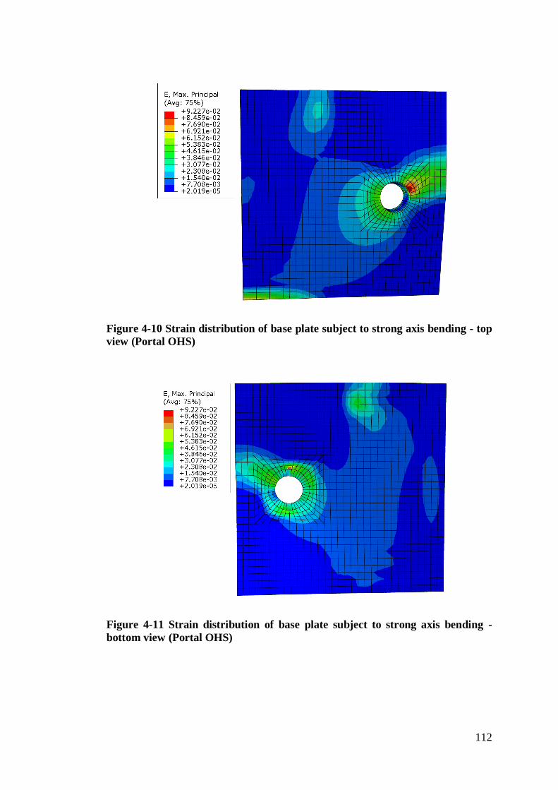
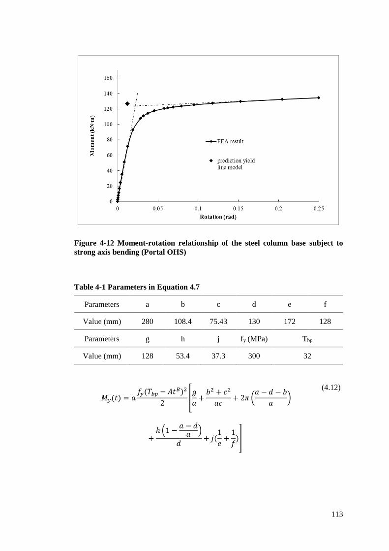


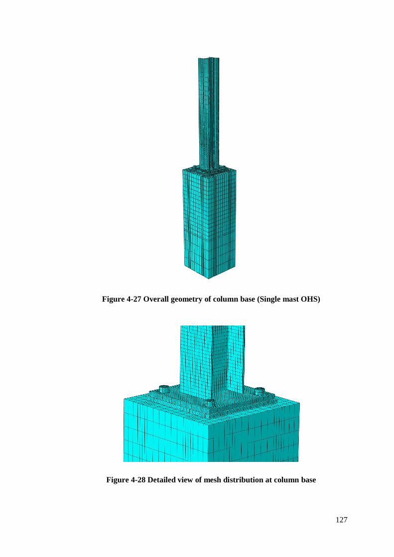


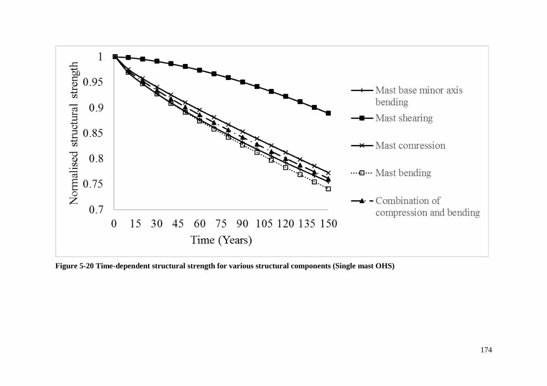
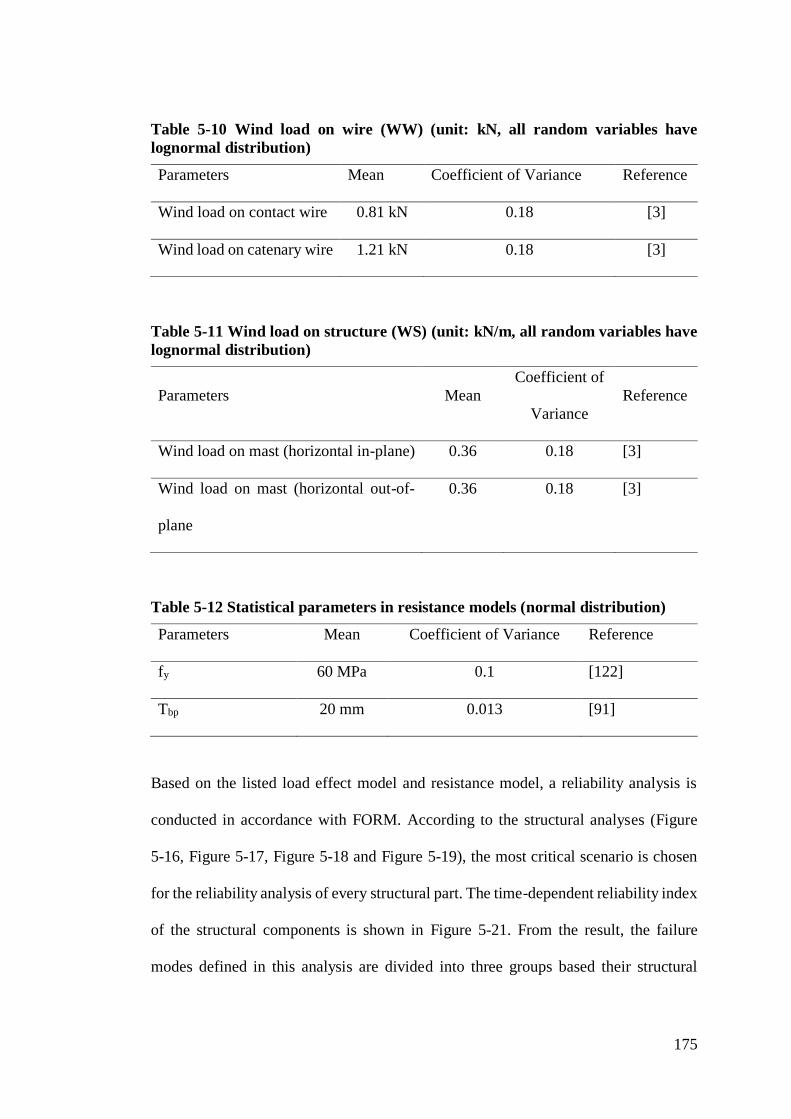


![PLEASE DO NOT REMOVE THIS PAGE - RMIT …researchbank.rmit.edu.au/eserv/rmit:38728/n2006067879.pdfdistances[17, 18], but an error-corrected repeater network with su cient bandwidth](https://static.documents.pub/doc/80x56/5f4b1ab468b0ac588c3e94b6/please-do-not-remove-this-page-rmit-38728n2006067879pdf-distances17-18-but.jpg)


