28
RELIABILITY ASSESSMENT OF STRUCTURAL DYNAMIC SYSTEMS DUE TO EARTHQUAKE- INDUCED TSUNAMIS Z. Shao & S.H. Cheung School of Civil and Environmental Engineering, NTU 07-Nov-2013 1

RELIABILITY ASSESSMENT OF STRUCTURAL DYNAMIC SYSTEMS DUE TO EARTHQUAKE-
INDUCED TSUNAMIS
Z. Shao & S.H. Cheung
School of Civil and Environmental Engineering, NTU
07-Nov-2013
1

Motivation
List of 10 COSTLIEST NATURAL HAZARDS from 1980 - 2012
Rank Overall loss [US$ mn] Fatalities Event Year
1. 210,000 15,840 Tohoku earthquake (JP) 2011
2. 125,000 1,322 Hurricane Katrina (US) 2005
3. 100,000 6,430 Kobe earthquake (JP) 1995
4. 85,000 84,000 Sichuan earthquake (CN) 2008
5. 65,000 210 Hurricane Sandy (US) 2012
6. 44,000 61 Northridge earthquake (US) 1994
7. 43,000 813 Thailand flood (SEA) 2011
8. 38,000 170 Hurricane Ike (US) 2008
9. 30,700 4159 China floods (CN) 1998
10. 30,000 520 Chile earthquake (CL) 2010
Source: Munich Re NatCatSERVICE 2

Motivation
List of 10 DEADLIEST TSUNAMIS in the history
Rank Death toll Location Year
1. 350,000 Indonesia (EQ) 2004
2. 100,000+ Ancient Greece (VC) 1410 B.C.
3. 100,000 Portugal (EQ) 1755
4. 100,000 Italy (EQ) 1908
5. 40,000 Taiwan (EQ) 1782
6. 36,500 Indonesia (VC) 1883
7. 30,000 Japan (EQ) 1707
8. 26,360 Japan (EQ) 1896
9. 25,674 Chile (EQ) 1868
10. 15,854 Japan (EQ) 2011
Source: Geist & Parsons 2011 Source: National Geophysical Data Center
EQ: earthquake; VC: volcano eruption 3

General Flowchart
1. Stochastic earthquake source modelling
2. Tsunami generation and propagation
3. Tsunami runup and wave-structure interaction
4. Reliability analysis and structural loss assessment
4

Earthquake Source Mechanism
• Far-field tsunami
– The amplitude of tsunami can be estimated reasonably well based
on the earthquake moment magnitude [Geist, 1999 and references therein]
• Near-field tsunami
– Slip distribution (uniform slip model, k-squared slip model, etc.)
– Fault dimension
– Fault geometry (slip angle, dip angle, strike angle)
– The above are also the important sources of uncertainties in
tsunami risk analysis
5

Tsunami Generation & Propagation
• Tsunami generation & propagation using COMCOT
(Cornell Multi-grid Coupled Tsunami Model)
– Initial water displacement calculation based on Okada’s
analytical solution for surface deformation in vertical
direction due to shear dislocation in a half space.
– Linear shallow water equations (SWE) and nonlinear
shallow water equations (NSWE).
– Explicit leap-frog finite difference method.
6

Tsunami-wave-structure Interaction
• Tsunami force classifications
– Hydrodynamic pressure
– Hydrostatic pressure
– Impact by debris
– etc.
• Simulation methods
– Monolithic & partitioned approaches
– ALE formulation (LS-DYNA)
Monolithic approach
Partitioned approach , ,( ) 0m
i j j i j ij j iv v v v f
7
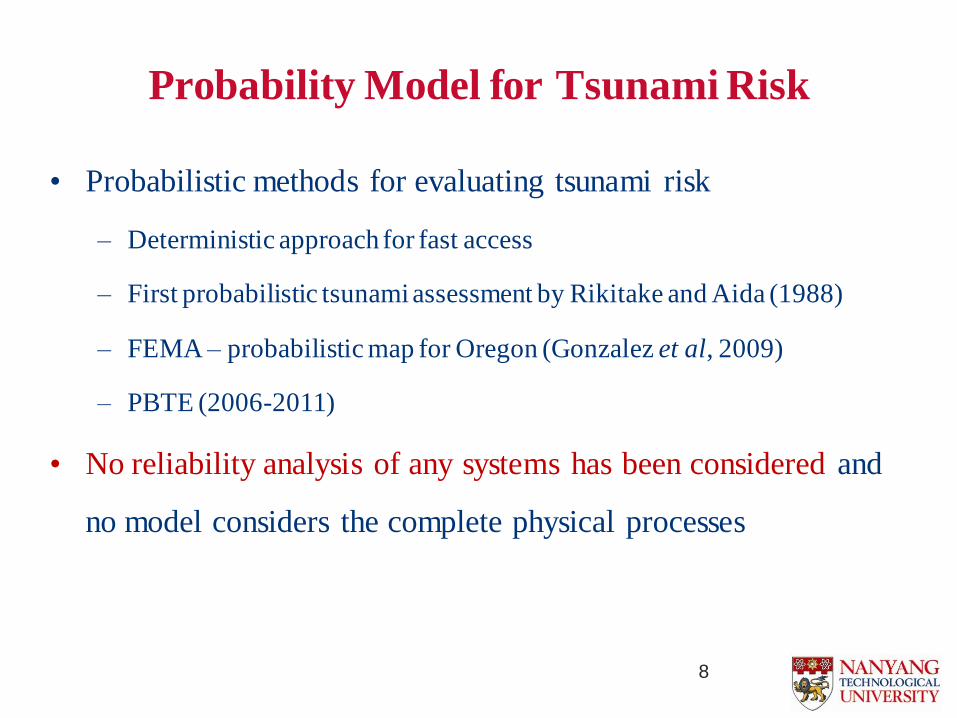
Probability Model for Tsunami Risk
• Probabilistic methods for evaluating tsunami risk
– Deterministic approach for fast access
– First probabilistic tsunami assessment by Rikitake and Aida (1988)
– FEMA – probabilistic map for Oregon (Gonzalez et al, 2009)
– PBTE (2006-2011)
• No reliability analysis of any systems has been considered and
no model considers the complete physical processes
8

Structural Reliability Analysis
• Structural reliability formulation
– The failure probability can be written in terms of a limit state
function L(θ) given by:
• Simulation methods for reliability analysis for general
nonlinear dynamic system involving high stochastic
dimension
– Monte Carlo
– Subset Simulation (Au and Beck, 2001)
– Competitive S3 and more efficient ADM (by Prof. Cheung and his
collaborators) and a new approach by Prof. Cheung and Sahil
9

Tohoku Tsunami Modelling • Tohoku tsunami (Mw 9.1) modeling: earthquake generation
Epicenter (Lat, Lon) [deg] 38.1, 143.2
Shao et al., 2011
Strike direction (θ) [deg] 199.0
Dip angle (δ) [deg] 10.0
Rake angle (λ) [deg] 92
Focal depth [m] 24400
Length of fault [m] 10^(-2.37+0.57*Mw) Blaster, 2010
Width of fault [m] 10^(-1.86+0.46*Mw) Blaster, 2010
Dislocation (slip) [m] Gallovic, 2004
Fault discretization 30 X 30 -
10

Tohoku Tsunami Modelling
Maximum inundation map (a) COMCOT simulation (b) Post-tsunami survey
observations and inundation lines (Source: Breanyn, Gusman et al. 2013)
(a) (b)
11

Tsunami & Structural Modelling
• Tsunami-wave-structure interaction using LS-DYNA
Geometry of the
structural wall [m]
Height 5
Length 7
Width 0.2
Water element size:
0.25m × 0.25m × 0.25m.
Structural wall
Air/Null Water part
12

Tsunami & Structural Modelling
• Material properties of the reinforced concrete
structural wall
Material parameters for concrete
MAT72 RL3
Mass density 2360 kg/m3
Elastic modulus Ec 27800 Mpa
Poisson ratio 0.2
34.5 MPa
Material parameters for steel rebar
MAT03
Mass density 7800 kg/m3
Young’s modulus Es 200 GPa
Poisson ratio 0.3
Yield’s strength 460 MPa
Percent reinforcement 2%
13

Stochastic Earthquake Parameter Modelling
• Earthquake parameter generation
Parameter Tohoku Region Earthquake Parameter for Mw 8.3
Epicenter (Lat, Lon) [deg] Fixed at 38.1, 143.2
Strike direction (θ) [deg] Fixed at 199.0
Dip angle (δ) [deg] Fixed at 10.0
Rake angle (λ) [deg] Normally distributed with a mean of 90 and a COV of 0.33*
Focal depth [m] Fixed at 24400
Length of fault [m] 10^(-2.37+0.57*Mw)**
Width of fault [m] 10^(-1.86+0.46*Mw)**
Dislocation (slip) [m]
Fault discretization 4 X 4
* Yamamoto & Hori, 2004;
** Blaster, 2010;
*** Gallovic, 2004. 14
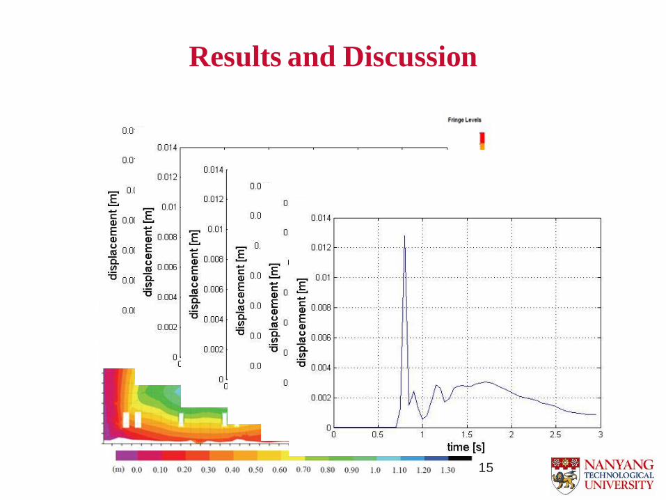
Results and Discussion
15

Problem Statement
• Computationally demanding in estimating the failure
probability in terms of a limit state function L(θ):
• MCS: 10/PF e.g. PF =10-3
• Subset Simulation: 500 * (-log(PF))
z(θ1)
z(θ2)
……
z(θNt)
Response
Performance Function
Numerical
simulations
Response Analysis
θ1
θ2
……
θNt
Stochastic
samples
Proposal Distribution
θi ∝ p(θ)
16

Problem Statement
• Computationally demanding in estimating the failure
probability in terms of a limit state function L(θ):
• MCS: 10/PF
• Subset Simulation: 500 * (-log(PF))
z(θ1)
z(θ2)
……
z(θNt)
Response
Performance Function
Response
Surface
Response Analysis
θ1
θ2
……
θNt
Stochastic
samples
Proposal Distribution
θi∝ p(θ)
RSM
RSM
17

Proposed Methodology
• Concept of the proposed method
Subset Simulation Algorithm
Modified Moving Least
Square Response Surface
SS-MLSRSA algorithm
18
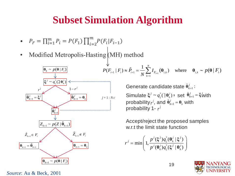
Subset Simulation Algorithm
Source: Au & Beck, 2001
*
*
( ) ( | )min 1,
( ) ( | )
j j
j k
j j j
k j k
j j
j
j
p qr
p q
ξ θ ξ
θ ξ θ
|~ ( )k iFpθ θ
*( | )~ j
j k
jq θξ
1
j j
k θ ξ 1 k
j
k θ θ
1
j
kθ
1k iZ F
1k i
FZ
1 ~ ( )ik p Fθ θ |
1 1
k k θ θ 1k k
θ θ
1 1~ ( | )k kZ p Z θ
jr 1
jr
j = 1 : N c
Generate candidate state
Simulate , set with
probability , and with
probability 1-
Accept/reject the proposed samples
w.r.t the limit state function
1 :j
kθ
*( | )~ j
j k
jq θξ 1
j j
k θ ξ
jr 1 k
j
k θ θj
r
11 1 , ,
1
1( | ) ) where( ( | )
i
N
i i i i k i k
k
F iP F F P IN
p F
θ θ θ
19

Modified Moving Least Square Response
Surface Approximation (MLSRSA)
Source: Taflanidis, A. A. & Cheung, S.-H., 2012
1
1 1
1
ˆ ( ) ( ) { } { }
[ ( ) ... ( )] [ ( ) ... ( )]
{ } [ ( ; ) ... ( ; ) ]
T T T
T T
NS NS
NS
f
f f
diag w d w d
θ b θ B W θ B B W θ F
B b θ b θ F θ θ
W θ θ θ θ θ
2 2
,
1
( ; )n
I I i i I i
i
d v
vθ θ θ θ θ θ
2
1
ˆ{ } { }[ ( ) ( )]NS
R I IIJ w f f
θ θ θ θ
2 2
2
1
1( ) if ; 0 else
1
k k
k
d
cD c
c
e ew d d D
e
w(d): weight measures depend on
the distance between support points
and interpolation point
d(θ;θI): norm distance with vi
represents importance of each
component of θ vector
20

Modified Moving Least Square Response
Surface Approximation (MLSRSA) (cont’d)
( ) ( )( ) ( ) ( )
( ) ( )
z pz p
z p d
θ θθ θ θ
θ θ θ
Source: Taflanidis, A. A. & Cheung, S.-H., 2012
( )( ( ) || ( )) ( ) log
( )
ire i i i i
i
D q dq
-4 -2 0 2 4 0
0.1
0.2
0.3
0.4
q(θ)
-4 -2 0 2 4 0
0.2
0.4
0.6
0.8
π(θ)
Gaussian kernel density
approximation of PDFs
ˆ( ) θ
21

General procedure of SS-MLSRSA
MCS • Stochastic NS ∝ p(θ)
• 𝜋(θ) ∝ p(θ|F1): Top 10% NS
Construct MLS
• Construct MLS surface
Stochastic sampling
• Stochastic Nmls ∝ p(θ)
• 𝜋(θ) ∝ p(θ|F2): Top 1% (NS+Nmls)
• 𝜋(θ) ∝ p(θ|F3): Top 0.1% (NS+Nmls)
• ……
22
• Naïve combination of Subset Simulation and MLSRSA…

General procedure of SS-MLSRSA
• Results and discussion
Smln Lv1 Lv2
350NS 2.1 -81.0
300NS 15.2 -25.0
250NS 24.0 -63.0
200NS 45.4 -39.0
Fit for the response surface model
based on the error (%) compared to
subset simulations
Threshold levels based on SS simulation:
b1= 0.75cm & b2 = 2.35cm
23

General procedure of SS-MLSRSA
Threshold lv 1
Threshold lv 2
MCS • Stochastic NS ∝ p(θ)
• 𝜋(θ) ∝ p(θ|F1): Top 10% NS
Construct MLS-lv1
• Stochastic Nmls ∝ p(θ)
• 𝜋(θ) ∝ p(θ|F1): Top 10% Nmls
Additional simulation Nsim =10% Nmls
• NS = Nmcs+Nsim
• 𝜋(θ) ∝ p(θ|F2): 10% Nsim+1% NS
Construct MLS-lv2 • Stochastic Nmls ∝ p(θ|F1)
• 𝜋(θ) ∝ p(θ|F2): Top 10% Nmls
24
• A NOVEL integration for them to communicate with each other to
obtain the performance as good as possible.

Results and Discussion
Top 10% of the maximum
displacement computed by
MLS-lv1 (theoretically, θ∝
p(θ|F1)) are selected and their
maximum displacements are computed using the original
physical numerical simulation
instead of using the response
surface.
The basic idea is to gain more
NS samples lying in the failure
domain for a more accurate
MLS-lv2. Failure probability curves for NS350 and SS
25

Results and Discussion
• Comparison of c.o.v. δ for SS and
SS-MLSRSA w.r.t MCS.
PF=10-2 Smln δ
SS 1,000 0.252
MCS 1,000 0.315
SS-MLSRSA 550 0.109
26
PF=10-2 SS MCS
SS-MLSRSA 10 20
SS - 2
• Factor of computational savings
PF=10-5 SS MCS
SS-MLSRSA 10 2500
SS - 250
• Factor of computational savings

Conclusions
• Tsunami-wave-structure interaction process simulation with credible
results using current numerical approaches.
• The proposed SS-MLSRSA approach based on a novel integration of
the SS algorithm and a recently proposed entropy-based MLSRSA
provides comparable failure probability estimates with much fewer
computational efforts compared with the SS without integrating with
the response surface approach.
27

THANK YOU
28


