Reliability of Pavement Structures Using Empirical ... Gossain and Manuel Page 2 INTRODUCTION The...

Reliability of Pavement Structures using Empirical-Mechanistic Models

by

J. A. Prozzi, Ph.D. (corresponding author)Assistant Professor

University of Texas at AustinDept. of Civil Engineering

1 University Station, C1761ECJ Hall 6.112

Austin, TX 78712-0278Phone: (512) 232-3488Fax: (512) 475-8744

[email protected]

Vishal GossainGraduate Research AssistantUniversity of Texas at Austin

Dept. of Civil Engineering1 University Station, C1761

ECJ Hall 6.154Austin, TX 78712-0278

L. Manuel, Ph.D.Assistant Professor

University of Texas at AustinDept. of Civil Engineering

1 University Station, C1761ECJ Hall 6.112

Austin, TX 78712-0278Phone: (512) 232-5691

Total number of words (4,052 words + 6 figures + 6 tables): 7,052

TRB 2005 Annual Meeting CD-ROM Paper revised from original submittal.

Prozzi, Gossain and Manuel Page 1

ABSTRACT

The National Cooperative Highway Research Program has undertaken a sizeable research effort

to develop a mechanistic-empirical design procedure for pavement structures: NCHRP 1-37A.

This procedure will likely replace the current AASHTO empirical design method, which has

been in use since the early 1970s. However, this change may take many years to materialize and

become widely accepted. One of the main improvements is the use of axle load spectra instead of

an aggregate measure of mixed traffic, such as the number of equivalent single axle loads

(ESALs). This change will considerably reduce the uncertainty in the pavement performance

estimations. In their present format, both the current AASHTO design method and the

forthcoming mechanistic procedure incorporate ad hoc procedures to assess design reliability.

The objective of this study is to develop and evaluate an alternative approach to assess this

reliability, and to highlight some important aspects that are often ignored.

Using Monte Carlo simulation techniques, the performance of a pavement structure designed

with the 1993 Guide with various levels of reliability under different traffic volumes is evaluated.

Effects of the environment, structural strength, and traffic volume on pavement reliability and

performance are discussed. The load models employed include consideration of the distribution

of loads by the actual load spectra measured in field. The reliability analysis results permit

discussion related to the implied reliability of the current AASHTO design method. An approach

to make the AASHTO design more robust is suggested. Another useful outcome of the present

study is the quantification of the relative influence on reliability of variables defining the loading

as well as the capacity. These findings might help identify critical areas to which resources

might be allocated to improve pavement reliability.



INTRODUCTION

The current AASHTO design equation for the design of flexible pavement structures (1) is

primarily based on the results of the AASHO Road Test, which took place in Ottawa, Illinois in

the late 1950s to early 1960s (2). The AASHO Committee on Design first published an interim

design guide in 1961. It was revised in 1972 (3) and 1981. In 1984-85, the Subcommittee on

Pavement Design and a team of consultants revised and expanded the guide under NCHRP

project 20-7/24 and issued the current guide in 1986 (1). The results of the AASHO Road test

were used to develop a deterioration model that has provided the basis for flexible and rigid

pavement design.

The original mathematical model chosen for both the flexible and rigid pavement analysis is

given by Equation 1.

( )β

ρ

−−= t

t

Wcccp 100 (1)

pt : serviceability value at time t ( ot cpc ≤≤1 )

c0 : initial serviceability value

c1 : serviceability level at which a test section was considered to have failed

Wt : accumulated axle load applications at the time t

β, ρ : regression parameters or functions.

Serviceability is defined as the ability of a specific section of pavement to serve traffic in its

existing conditions (4). Equation 1 estimates pt in terms of Present Serviceability Index (PSI),

defined as a mathematical combination of values obtained from certain distress measurements so

formulated as to predict the Present Serviceability Rating (PSR) for those pavements within

prescribed limits (4). PSR is the mean of the individual ratings (by individuals of a specific

panel) of the present serviceability of a specific section of roadway. The individual ratings varied

between 5 (Excellent) to 0 (Very Poor). Equation 2 was used by AASHO to determine PSI (2).

( ) 238.101.01log91.103.5 RDPCSVpt −+−+−= (2)



SV : mean of the slope variance

C : linear cracking

P : patching area

RD : average rut depth

β and ρ are given by Equations 3 and 4.

( )( ) 31

2

2

21

14.0

BB

Bo

LD

LLB

++

+=β(3)

( )( ) 2

31

21

20 1A

AA

LL

LDA

++

=ρ(4)

332211 DaDaDaD ++= (5)

D1 : surface thickness (in)

D2 : base thickness (in)

D3 : subbase thickness (in)

L1 : nominal axle load in kips

L2 : axle type (1 for single axles and 2 for tandem axles)

ai : layer coefficients.

It was found that designs failing early tended to have an increasing rate of serviceability loss,

while more adequate designs as a rule had a decreasing loss rate. The function ρ is equal to the

number of load applications at which pt = 1.5 (failure condition). The regression equations for ρ,

β and pt were obtained using a stepwise regression approach, which did not account for

unobserved events. In addition, there are serious inconsistencies in the specification of the

regression equations for β and ρ. These two aspects have led to the estimation of biased

regression parameters. Finally, all the models are intrinsically linear leading to unnecessary large

regression errors. The estimated standard error of Equation 1 was approximately 0.707 PSI (5).

Current AASHTO design equations

After estimating the regression parameters, Equations 6 and 7 were developed for flexible

pavements (2).



( )( ) 23.3

219.5

23.321

1

081.04.0

LD

LL

++

+=β(6)

)log(33.4)log(79.4)1log(36.993.5log 221 LLLSN ++−++=ρ (7)

SN : structural number of the pavement given by Equation 8

332211 DaDaDaSN ++= (8)

All other variables are previously defined.

The procedure is simplified if an equivalent 18 kip (80 kN) single axle load is used. By

combining Equations 1, 6 and 7 and setting L1 = 18 and L2 = 1, Equation 9 is obtained.

( )( ) 19.5

18

1

10944.0

5.12.4

2.4log

2.01log36.9log

++

−

−

+−+=

SN

p

SNW

f

t (9)

Wt18 : number of 18 kip (80 kN) single axle load applications to time t

pf : the terminal serviceability index.

Equation 9 is applicable only to flexible pavements in the AASHO Road Test with an effective

subgrade resilient modulus of 3,000 psi (20.7 MPa).

The original equations were developed under a given climatic setting with a specific set of

pavement materials and subgrade soils. The climate at the test section was temperate with an

average annual precipitation of about 34 in (864 mm). The average depth of frost penetration was

about 28 in. (711 mm). The subgrade soils consisted of A-6 and A-7-6 that were poorly drained

with CBR values ranging from 2 to 4.

For other subgrade and environmental conditions, Equation 9 was later modified to Equation 10

( )( )

( ) 07.8log32.2

1

10944.0

5.12.4

2.4log

2.01log36.9log

19.5

18 −+

++

−

−

+−+= R

f

t M

SN

p

SNW (10)



MR = the effective roadbed soil resilient modulus. To take local precipitation and drainage

conditions into account, Equation 8 was modified to Equation 11.

33322211 DmaDmaDaSN ++= (11)

m2 : drainage coefficient of base course.

m3 : drainage coefficient of subbase course.

Equation 10 is the performance equation which gives the allowable number of 18 kip single axle

load applications Wt18 to cause the reduction of PSI to pf. If the predicted number of applications

Wt18 is equal to W18 (expected traffic in ESALs), the reliability of the design is only 50%

because all variables in Equation 10 predicts pavement performance conditional on mean values

of the design variables. To achieve a higher level of confidence in the designs, W18 must be

smaller than Wt18 by a normal deviate ZR given by Equation 12.

0

1818 loglog

S

WWZ t

R

−=

(12)

Where ZR is the normal deviate for a given reliability R and S0 is overall standard deviation,

which accounts for the variability of all variables. Combining Equations 10 and 12 and replacing

(4.2 – pf) by ∆PSI yields Equation 13, which is the current final design equation for flexible

pavements.

( )( )

( ) 07.8log32.2

1

10944.0

5.12.4

2.4log

2.01log36.9log

19.5

018 −+

++

−

−

+−++= R

f

Rt M

SN

p

SNSZW (13)

The DNPS86 computer program issued by AASHTO can be used to solve Equation 13 along

with the nomograph provided by AASHTO 1993. Table 1 shows the percentage distribution of

overall variance when the AASHTO equations are used for pavement design as provided by

AASHTO 1986. Applications of the reliability concept require the selection of a standard

deviation that is representative of local conditions. It is suggested that standard deviations of 0.45

be used for flexible pavements and 0.35 for rigid pavements (4).

Non-linear Model



In order to address some of the shortcomings identified with the original AASHTO deterioration

model (Equation 1), on which the current AASHTO design equation is based (Equation 13), a

more accurate and statistically sound nonlinear deterioration model has been recently developed

(5). This model was developed using the same data set and the same number explanatory

variables, while relaxing the linear specification restriction and accounting for unobserved

events. The model also employed a simultaneous estimation approach rather than a stepwise

approach. A random effects approach was used for the estimation of the regression parameters

resulting in an estimated combined standard error of 0.377 PSI, which is approximately half the

standard error of the original model. By addressing these problems, the parameter estimates are

unbiased.

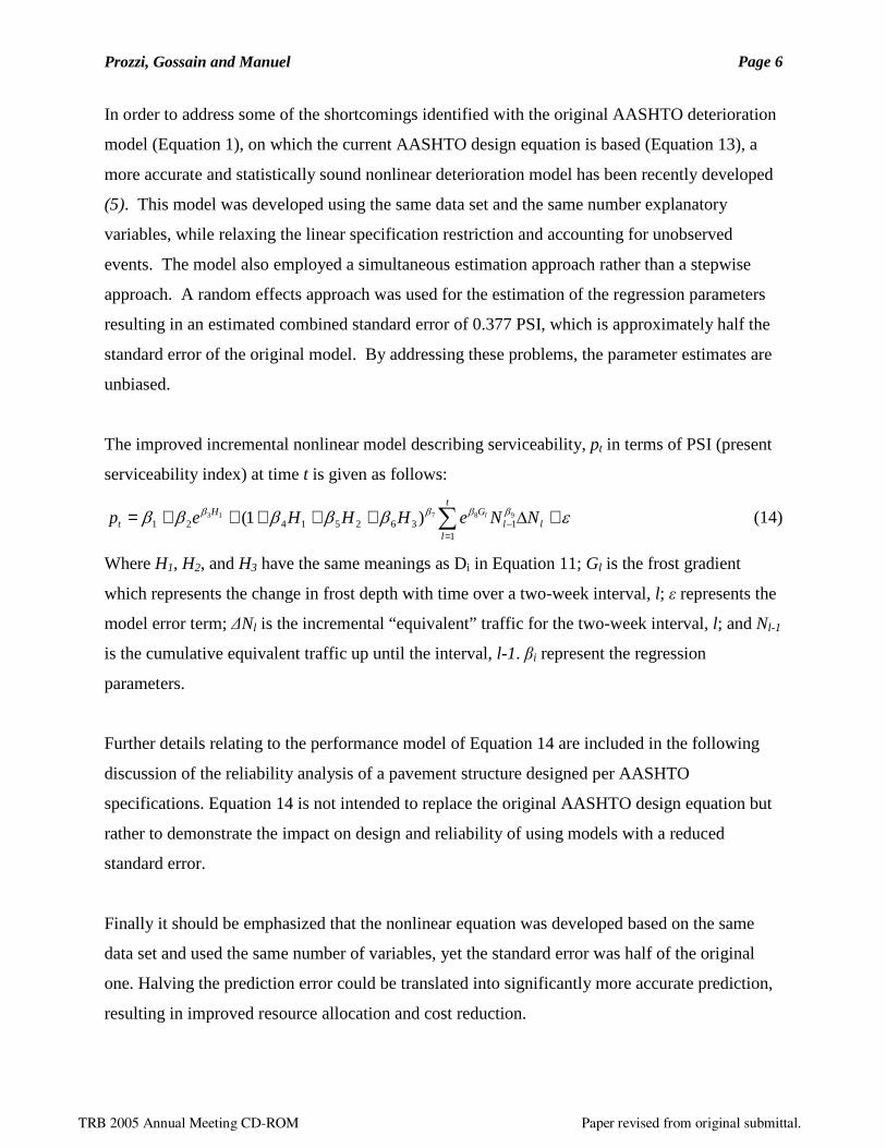
The improved incremental nonlinear model describing serviceability, pt in terms of PSI (present

serviceability index) at time t is given as follows:

∑=

− +∆+++++=t

lll

GHt NNeHHHep l

113625142198713 )1( εβββββ ββββ (14)

Where H1, H2, and H3 have the same meanings as Di in Equation 11; Gl is the frost gradient

which represents the change in frost depth with time over a two-week interval, l; ε represents the

model error term; ∆Nl is the incremental “equivalent” traffic for the two-week interval, l; and Nl-1

is the cumulative equivalent traffic up until the interval, l-1. βi represent the regression

parameters.

Further details relating to the performance model of Equation 14 are included in the following

discussion of the reliability analysis of a pavement structure designed per AASHTO

specifications. Equation 14 is not intended to replace the original AASHTO design equation but

rather to demonstrate the impact on design and reliability of using models with a reduced

standard error.

Finally it should be emphasized that the nonlinear equation was developed based on the same

data set and used the same number of variables, yet the standard error was half of the original

one. Halving the prediction error could be translated into significantly more accurate prediction,

resulting in improved resource allocation and cost reduction.



RELIABILITY ANALYSIS OF A PAVEMENT STRUCTURE DESIGNED PER

AASHTO SPECIFICATIONS

The reliability of a specific pavement structure was investigated using the performance model

given by Equation 14. The objective was to assess the actual reliability of the pavement

structure which is designed with a specific reliability according to AASHTO 1993 method.

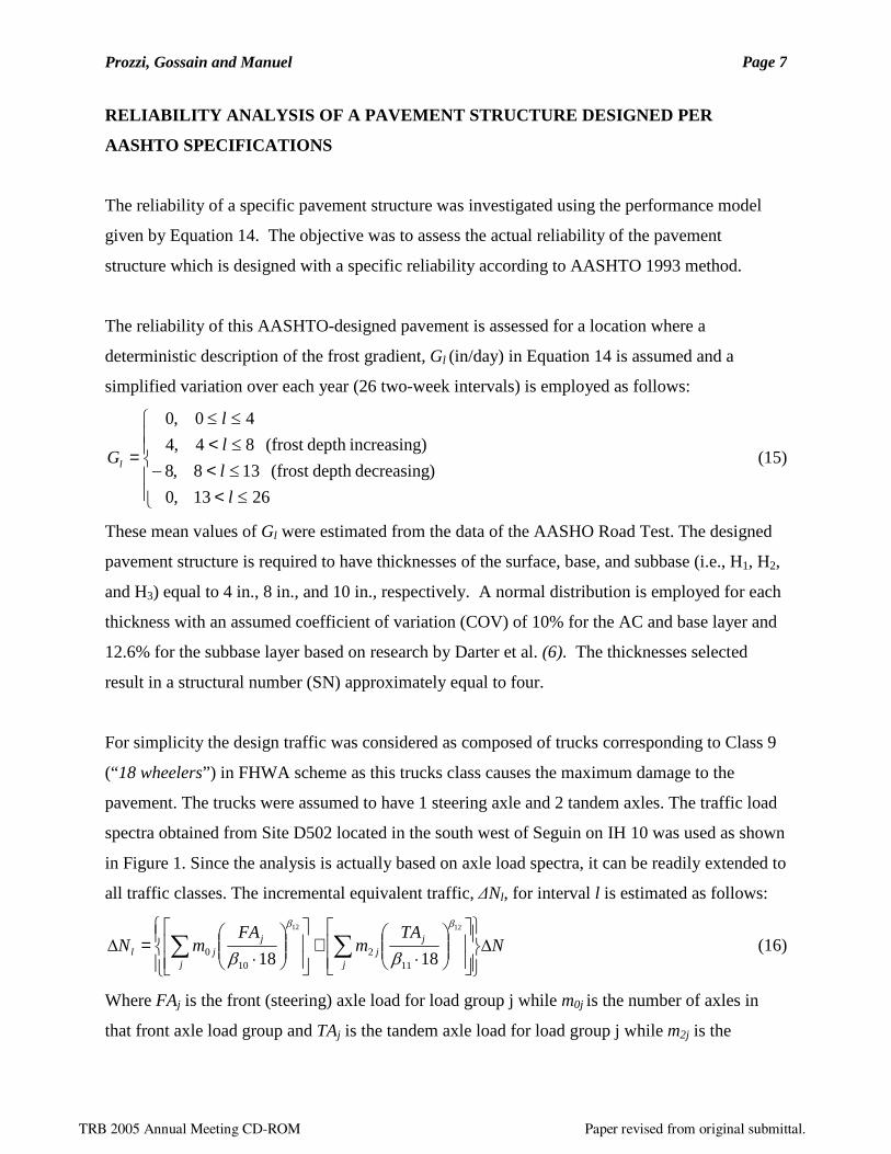
The reliability of this AASHTO-designed pavement is assessed for a location where a

deterministic description of the frost gradient, Gl (in/day) in Equation 14 is assumed and a

simplified variation over each year (26 two-week intervals) is employed as follows:

≤<≤<−≤<≤≤

=

2613,0

)decreasingdepth (frost 138,8

)increasingdepth (frost 84,4

40,0

l

l

l

l

Gl (15)

These mean values of Gl were estimated from the data of the AASHO Road Test. The designed

pavement structure is required to have thicknesses of the surface, base, and subbase (i.e., H1, H2,

and H3) equal to 4 in., 8 in., and 10 in., respectively. A normal distribution is employed for each

thickness with an assumed coefficient of variation (COV) of 10% for the AC and base layer and

12.6% for the subbase layer based on research by Darter et al. (6). The thicknesses selected

result in a structural number (SN) approximately equal to four.

For simplicity the design traffic was considered as composed of trucks corresponding to Class 9

(“18 wheelers”) in FHWA scheme as this trucks class causes the maximum damage to the

pavement. The trucks were assumed to have 1 steering axle and 2 tandem axles. The traffic load

spectra obtained from Site D502 located in the south west of Seguin on IH 10 was used as shown

in Figure 1. Since the analysis is actually based on axle load spectra, it can be readily extended to

all traffic classes. The incremental equivalent traffic, ∆Nl, for interval l is estimated as follows:

NTA

mFA

mNj

jj

j

jjl ∆

⋅

+

⋅

=∆ ∑∑1212

1818 112

100

ββ

ββ(16)

Where FAj is the front (steering) axle load for load group j while m0j is the number of axles in

that front axle load group and TAj is the tandem axle load for load group j while m2j is the



number of axles in that load group. The number of axles for each load group is for a two-week

interval. ∆N is the truck traffic for every two weeks. The cumulative equivalent traffic in

Equation 14 is given as follows:

∑−

=− ∆=

1

11

l

qql NN (17)

The regression parameters, β1 – β 12, in Equations 14 and 16 that were estimated using a random

effects approach are listed in Table 2.

Information on the various random variables required for the simulation-based reliability

analysis is summarized in Table 3. Note that the model error term, ε, in the performance

deterioration model of Equation 14 is modeled as normal random variable with a zero mean and

a standard deviation of 0.377. This is consistent with the assumptions of the classical regression

model used for the development of the model.

EXAMPLE OF SUMULATED LOADING AND PERFORMANCE

A terminal value of 2.5 is considered with the serviceability model of Equation 14. Thus, when

pt falls below 2.5, the pavement is assumed to have failed. Monte Carlo simulations for a

duration of ten years for the different levels of design reliability are conducted using the random

variable information in Table 3 in combination with the performance model of Equation 14.

The analysis focuses primarily on determining how different the predicted reliability of an

AASHTO-designed pavement structure is from the reliability based on the more accurate

nonlinear model. The influence of various parameters related to loading, climate, and structure

on the performance and reliability of the selected pavement structure are also assessed.

Three different cases of design reliability corresponding to 50%, 80% and 90% were considered

for the analysis.

Loading

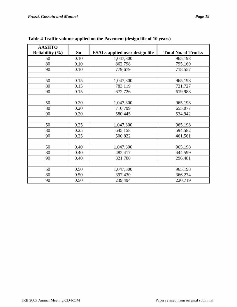
Table 4 shows the different cumulative traffic volumes applied on the pavement over the

duration of design life corresponding to different levels of reliability and different values of S0.



Performance

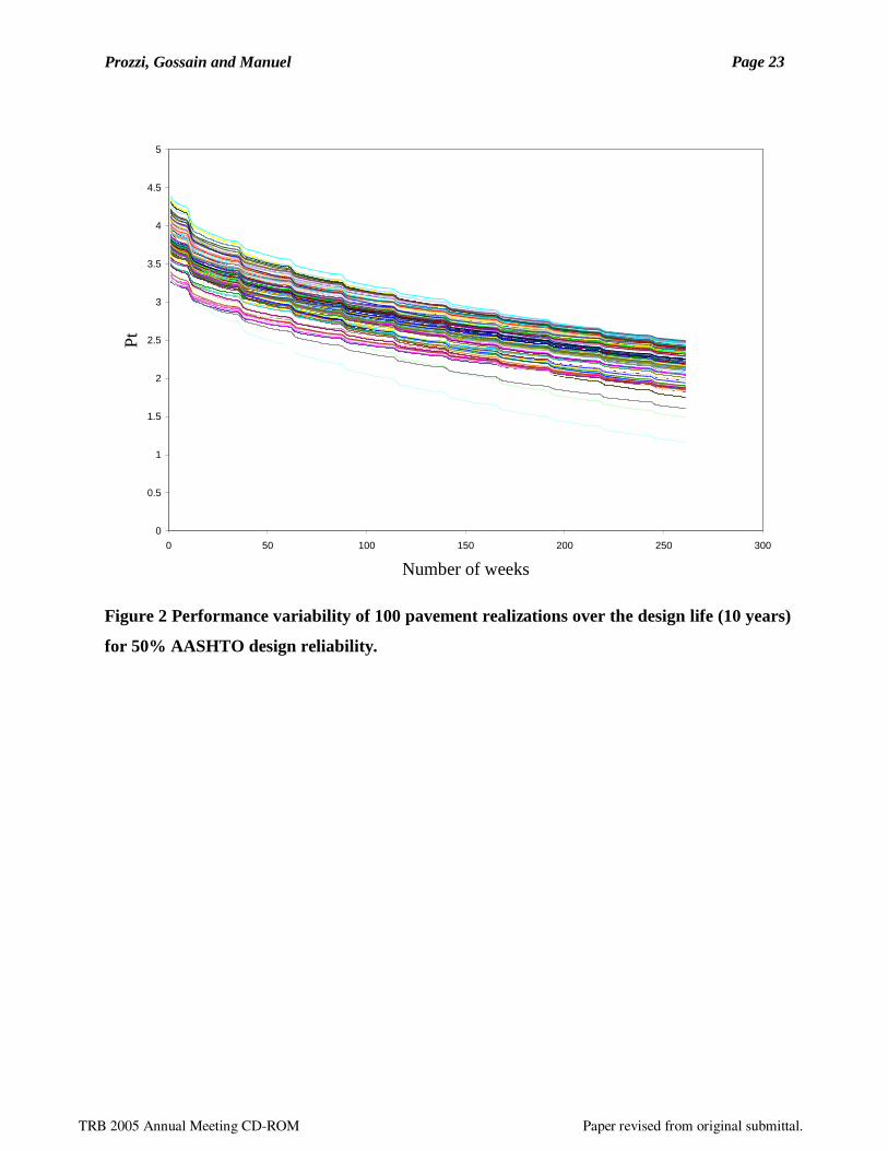
As an example, Figure 2 shows 100 realizations of the serviceability, pt, as a function of time for

the AASHTO design reliability of 50% and S0 = 0.5. For a terminal serviceability, pf, of 2.5, it is

seen that a fraction of the pavements fail within ten years. An expanded discussion about

pavement performance based on a larger number of simulations is presented in the following

section. It is worthy noting the steps observed in the performance predictions, which correspond

to the thawing periods.

RESULTS

The performance of the selected pavement structure was evaluated using Monte Carlo

simulations. Table 5 depicts the number of simulations carried out and the corresponding

reliabilities of the pavements for the various cases considered. The number of simulations

required is stated with a confidence level of 95% and an error range of ±1%.

AASHTO recommends values of S0 from 0.4 to 0.5 (1). As is evident from Table 5, the actual

reliabilities obtained for this range are very high as compared to the design reliabilities. This

large discrepancy between AASHTO’s implied reliability for the chosen design and the

simulation-based reliability estimate is attributed to the fact that a more accurate performance

model is used here in conjunction with a more accurate traffic characterization. Recall that the

estimated standard error of the original AASHTO design equation was 0.707 PSI, while the

standard error for the nonlinear model in Equation 14 is 0.377 PSI. From the above, it would

appear that the approach incorporated in the AASHTO design procedure is conservative or,

equivalently, that AASHTO designs may be more reliable than the procedure suggests.

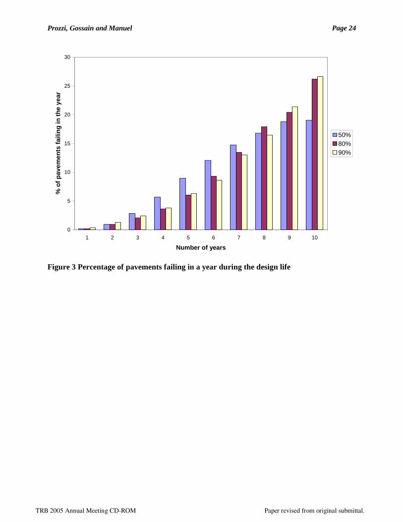
Figure 3 demonstrate that the simulations with the nonlinear model capture the pavement

behavior efficiently. As the design reliability is increased for the pavement with the same S0, the

number of pavement failures in the early years should reduce and those in the later years should

increase, which is consistent with the results obtained as depicted in Figure 3. It is also evident

from the simulation results that a reduction in the value of S0 causes the actual reliability to be

closer to the design reliability. It should be noted that changing the value of S0 also changes the



design traffic for the pavement. It was found that a value of 0.2 for S0 (much lower than the

range suggested by AASHTO) would be better as it reduces the gap between actual and design

reliabilities as determined by the simulation and depicted in Table 5. Thus changing the value of

S0 can be a way by which the AASHTO equation can be made robust and accurate.

EFFECT OF DESIGN VARIABLE ON PERFORMANCE

Aggregated Effect on Time to Failure based on Regression Analysis

In order to establish which design variables exert the largest influence on pavement performance,

a regression analysis was carried out to estimate time to failure (Tf) of the pavement structures

(that actually failed) as a function of the design variables. The following second-order surface

was used to fit the data:

314131211

1092

82

72

62

543210

1213

3221321321

HHHHH

HHHHHHHf

ZZZZZZZZ

ZZZZZZZZZZZZTHHH

αααα

ααααααααααα

εεε

ε ε

++++

++++++++++=(19)

Where the variables, Z(.), represent the number of standard deviations from their respective

means of the variables, H1, H2, H3 and ε (all normal), as described before. The parameter

estimates (α 0 – α 14) are given in Table 6 along with their t-statistics for the design reliability of

50% and S0 = 0.5. By expressing the values of the random variables in terms of standardized

deviations from their means, the parameter estimates in Table 6 make comparison of the

influence of each variable on pavement performance easier.

Based on the parameter estimates given in Table 6, the first-order effects of the variables can be

summarized by three broad statements:

1. The variables, H1 (surface thickness) and ε (model error), have the largest influence on

pavement performance. If the surface thickness is sampled one standard deviation below

its mean it will, on the average, cause a reduction in pavement life of approximately three

years. On the other hand, if the model error is sampled one standard deviation below its

mean it will, on the average, cause a reduction in pavement life of approximately five

years



2. The variables H2 and H3 (representing base and subbase thicknesses, respectively) are

clearly seen to have the smallest effect of performance. When they take on values that

are one standard deviation below their means they reduce the pavement life by

approximately one and a half years, on average.

Of the ten second-order terms in Equation 19, the largest second-order influence results from the

product terms involving surface thickness, H1, and model error, ε. Similar results were obtained

for all the cases considered as depicted in Table 4.

The findings from these simulation studies suggest that, to increase pavement life, placing

stricter quality control on the surface thickness might pay off twice as much, on average, than

controlling the base and subbase thicknesses. However, the model error is seen to be almost as

important. This suggests that efforts directed towards establishing accurate performance models

might translate directly into better predictions of time to failure and reliability.

Analysis of Early and Late Failures

Once the relative effects on performance of the pavement structure were assessed for the various

design variables, a more in-depth analysis was carried out to determine which variables were

responsible for early failures and which for later ones. Early failures are usually attributed to

poor construction practices without any further quantification or understanding of what causes

these failures.

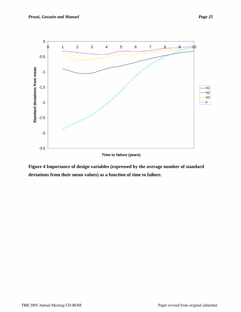
The 27,336 failed pavements were grouped into ten categories according to the year in which

they failed for the case of design reliability of 50% and S0 value of 0.5. Within each group, the

average of each of the design variables was determined. The averages of these various design

variables (expressed as standardized deviations from their mean values) are represented in Figure

4 for years 1 to 10.

Figure 4 reveals that for the failed pavements, two random variables show relatively uniform

variation with time in their averages. For example, the failed pavements had base and subbase

thicknesses (H2 and H3) on the order of half a standard deviation below their respective mean



values for all failed pavements uniformly over the ten years. Two variables, surface thickness

(H1) and model error (ε), however, displayed systematic variations with time. Considering the

model error first, it can be seen that the early failures seem to result when the model error is very

far below its mean (as many as 2 to 3 standard deviations on average in the first three years).

Also, in the early years, surface thickness (H1) among failed pavements was generally between 1

and 1.5 standard deviations below its mean value. Note however that among these early failures,

it was generally the case that only one of these two random variables needed to be sampled

significantly below its mean value for a failure to result. To explain this further, for the 1,106

early failures (or approximately 4.1% of all failures) where the time to failure, Tf, was less than 3

years, the sample correlation coefficient between ε and H1 was large but negative. This is show

graphically in Figure 5.

Although a very small number of pavements failed in the early years, these failures may be

attributed to limited understanding of the inherent variability in pavement performance as

reflected by performance model error. Otherwise, early failures may be generally attributed to

lower surface thickness values than recommended.

As can be seen in Figure 4, in later years, the importance of the model error (ε) is diminished

greatly. It is seen to have a noticeable trend with time. Late failures are generally less sensitive

to modeling uncertainty. The surface thickness, H1, is also seen to be of less importance among

the later failures than it was for early failures. To contrast early failures with later ones in the

light of the most important source of variability (model uncertainty) as well as to point out the

importance of the frost gradient term, Gl, one might examine Figure 6. It may be seen as

expected that there are systematic seasonal clusters of failures that occur over the five years

shown in the figure. This characteristic results from the effect of the deterministic frost gradient

modeled annually according to Equation 15, and reflects what was observed at the AASHO Road

Test.

Finally, it may be noted that the rate of occurrence of failures increases with time as the traffic

load cycles compromise the pavement’s performance. Similar results were obtained for the rest

of the cases considered.



CONCLUSIONS

Using simulation techniques, the reliability of a selected pavement structure has been studied.

The design for this structure was based on the current AASHTO design approach and was

designed with 50%, 80% and 90% reliability with overall standard deviations varying from 0.1 to

0.5. Results from the simulation studies that employed a nonlinear performance model with

reduced standard error suggest that the reliabilities were higher for the values of standard

deviation recommended by AASHTO, implying that the AASHTO design approach might be

overly conservative when axle load spectra are used. An overall standard deviation of around 0.2

could be used to reduce the gap between the design and actual reliabilities, especially in those

cases where accurate expected traffic information is available. It was also demonstrated that the

simulations capture the pavement behavior satisfactorily.

A detailed examination of the failed pavements showed that the parameters that influence

pavement performance to the greatest extent are the surface asphalt thickness and the model error.

This supports the idea that most simulation approaches that do not account for model error are

ignoring an important component of the overall performance variability.

When time to failure is studied, it is found that early failures may be attributed to either model

error (ε) or to surface thickness (H1) – sampling of these random variables two or more standard

deviations below their means often caused early failures. Since model error is inherent to the

modeling process and can not be avoided, during the construction process all possible resources

should be utilized to control the variability of the thickness of the surface layer.

ACKNOWLEDGEMENTS

The authors gratefully acknowledge the financial support from the Texas Department of

Transportation as part of the project, “Evaluate Equipment, Methods, and Pavement Design

Implications of the AASHTO 2002 Axle-Load Spectra Traffic Classification Methodology for

Texas Conditions,” directed by Joe Leidy and coordinated by German Claros.



REFERENCES

1. AASHTO, 1993. AASHTO Guide for Design of Pavement Structures, American

Association of Transportation and Highway Officials, Washington, DC.

2. HRB, 1962. The AASHO Road Test, Report 5: Pavement Research, Special Report 61E,

Highway Research Board, Washington, DC.

3. ASHTO, 1972. AASHTO Interim Guide for Design of Pavement Structures, American

Association of Transportation and Highway Officials, Washington, DC.

4. Huang, Y. H., 1993. Pavement Analysis and Design, Prentice-Hall, Inc., New Jersey.

5. Prozzi, J. A. and S.M. Madanat. A Nonlinear Model for Predicting Pavement Serviceability,

Proceedings of the Seventh International Conference Applications of Advanced Technology

in Transportation, American Society of Civil Engineering, pp. 481-488, Boston, MA, 2002.

6. Darter, M. I., Hudson, W. R., and Brown, J. L., 1973. Statistical Variations of Flexible

Pavement Properties and their Consideration in Design, Proceedings, Association of Asphalt

Pavement Technologists, Vol. 42, pp. 589-613.



LIST OF TABLES

Table 1 Percentage distribution of overall variance

Table 2 Estimates of Parameters in Nonlinear Model based on a Random Effects Approach.

Table 3 Random Variables included in the Simulation Studies.

Table 4 Traffic volume Applied on the pavement (design life of 10 years)

Table 5 Monte Carlo Simulations for the Pavement.

Table 6 Parameter estimates and corresponding t statistics for a second-order response surface

for time to failure (n= 26,866; R2 = 0.988; standard error = 5.77).

LIST OF FIGURES

Figure 1 Load spectra as obtained from the field

Figure 2 Performance variability of 100 pavement realizations over the design life (10 years)

for 50% AASHTO design reliability.

Figure 3 Percentage of pavements failing in a year during the design life

Figure 4 Importance of design variables (expressed by the average number of standard

deviations from their mean values) as a function of time to failure.

Figure 5 Variation of model error and surface thickness among pavements that experienced early

failures.

Figure 6 Variation of model error with time to failure for the failed.



Table 1 Percentage Distribution of overall variance

Type of

prediction

Source of

Variance

Value Flexible

pavement

Value Rigid

pavement

Traffic factor 14% 22%

Unexplained 3% 4%

Lack of fit 1% 1%

Traffic

prediction

Total Variance 0.0429 18% 0.0429 27%

Design Factor 45% 42%

Unexplained 5% 8%

Lack of fit 32% 23%

Performance

Prediction

Total Variance 0.1938 82% 0.1128 73%

Overall

Variance

0.2367 100% 0.1557 100%



Table 2 Estimates of Parameters in Nonlinear Model based on a Random Effects

Approach.

Parameter Random Effects Estimate

β1 4.24

β 2 -1.43

β 3 -0.856

β 4 1.39

β 5 0.329

β 6 0.271

β 7 -3.03

β 8 -0.173

β 9 -0.512

β 10 0.552

β 11 1.85

β 12 4.15



Table 3 Random Variables included in the Simulation Studies.

Random Variable Distribution Parameters

H1 Normal Mean = 4 in. (100 mm), CoV = 10%

H2 Normal Mean = 8 in. (200 mm), CoV = 10%

H3 Normal Mean = 10 in. (250 mm), CoV = 12.6%

ε Normal Mean = 0, std. dev. = 0.377

∆N Normal CoV = 15%



Table 4 Traffic volume applied on the Pavement (design life of 10 years)

AASHTO Reliability (%) So ESALs applied over design life Total No. of Trucks

50 0.10 1,047,300 965,19880 0.10 862,798 795,16090 0.10 779,679 718,557

50 0.15 1,047,300 965,19880 0.15 783,119 721,72790 0.15 672,726 619,988

50 0.20 1,047,300 965,19880 0.20 710,799 655,07790 0.20 580,445 534,942

50 0.25 1,047,300 965,19880 0.25 645,158 594,58290 0.25 500,822 461,561

50 0.40 1,047,300 965,19880 0.40 482,417 444,59990 0.40 321,700 296,481

50 0.50 1,047,300 965,19880 0.50 397,430 366,27490 0.50 239,494 220,719



Table 5 Monte Carlo Simulations for the Pavement

AASHTO

Reliability

(%)

So Number of

simulations

Number

of

failures

Actual

Reliability

(%)

Actual

Simulations

required

50 0.1 93,000 27,336 70.6 92,279

80 0.1 160,000 32,140 79.9 152,827

90 0.1 300,000 49,414 83.5 194,813

50 0.15 93,000 27,336 70.6 92,279

80 0.15 250,000 41,230 83.5 194,521

90 0.15 300,000 35,319 88.2 287,889

50 0.2 93,000 27,336 70.6 92,279

80 0.2 300,000 39,737 86.7 251,610

90 0.2 475,000 39,471 91.7 423,887

50 0.25 93,000 27,336 70.6 92,279

80 0.25 350,000 37,398 89.3 320,947

90 0.25 638,500 36,353 94.3 636,318

50 0.4 93,000 27,336 70.6 92,279

80 0.4 790,000 40,735 94.8 706,610

90 0.4 2,250,000 39,936 98.2 2,125,946

50 0.5 93,000 27,336 70.6 92,279

80 0.5 1,250,000 38,704 96.9 1,202,282

90 0.5 5,000,000 39,462 99.2 4,829,051



Table 6 Parameter estimates and corresponding t statistics for a second-order response

surface for time to failure (n= 26,866; R2 = 0.988; standard error = 5.77).

Non-standardized Coefficients

Standardized Coefficients

B Std. Error Betat

(Constant) 348.2 0.196 1774.1H1 83.5 0.155 1.468 540.1H2 36.5 0.104 0.678 352.9H3 47.8 0.114 0.884 420.0E 132.3 0.225 1.902 588.7

H12 4.5 0.039 0.140 116.2

H22 0.9 0.028 0.025 32.9

H32 1.6 0.030 0.045 52.6

e2 9.7 0.064 0.303 151.4H1 H2 4.4 0.048 0.092 93.0H2 H3 2.4 0.041 0.047 58.0H3 e 13.7 0.067 0.307 203.0e H1 23.1 0.084 0.511 275.6e H2 10.4 0.063 0.235 164.7

H1 H3 5.9 0.050 0.122 117.6



0

0.05

0.1

0.15

0.2

0.25

0.3

0.35

0 10 20 30 40 50 60 70 80 90

Axle load

No

rmal

ized

Fre

qu

ency

Steering AxleTandem Axle

Figure 1 Load Spectra (in kips) as obtained from the field



0

0.5

1

1.5

2

2.5

3

3.5

4

4.5

5

0 50 100 150 200 250 300

Number of weeks

Pt

Figure 2 Performance variability of 100 pavement realizations over the design life (10 years)

for 50% AASHTO design reliability.



0

5

10

15

20

25

30

1 2 3 4 5 6 7 8 9 10

Number of years

% o

f p

avem

ents

fai

ling

in t

he

year

50%80%90%

Figure 3 Percentage of pavements failing in a year during the design life



-3.5

-3

-2.5

-2

-1.5

-1

-0.5

0

0 1 2 3 4 5 6 7 8 9 10

Time to failure (years)

Sta

nd

ard

dev

iati

on

s fr

om

mea

n

H1H2H3e

Figure 4 Importance of design variables (expressed by the average number of standard

deviations from their mean values) as a function of time to failure.



-5

-4

-3

-2

-1

0

1

2

3

-5 -4.5 -4 -3.5 -3 -2.5 -2 -1.5 -1 -0.5 0 0.5

Number of st. dev. from the mean of e

Nu

mb

er o

f st

. dev

. fro

m t

he

mea

n o

f H

1

Early Failures : 0 < Tf < 3 years

Sample Correlation Coefficient = -0.66015

Figure 5 Variation of model error and surface thickness among pavements that

experienced early failures.



-2

-1.5

-1

-0.5

0

0.5

0 20 40 60 80 100 120 140

Number of periods to failure (bi weekly period)

Nu

mb

er o

f st

. dev

. fro

m t

he

mea

n f

or

e

Figure 6 Variation of model error with time to failure for the failed pavements


Date post:	12-Jun-2018
Category:	Documents
Upload:	truongnga
View:	220 times
Download:	0 times

Reliability of Pavement Structures Using Empirical ... Gossain and Manuel Page 2 INTRODUCTION The...

Documents