Remember Where You Came From: On The Second-OrderRandom Walk Based Proximity Measures

Yubao Wu, Yuchen Bian, Xiang ZhangDepartment of Electrical Engineering and Computer Science, Case Western Reserve University

{yubao.wu, yuchen.bian, xiang.zhang}@case.edu

ABSTRACTMeasuring the proximity between different nodes is a fun-damental problem in graph analysis. Random walk basedproximity measures have been shown to be effective andwidely used. Most existing random walk measures are basedon the first-order Markov model, i.e., they assume that thenext step of the random surfer only depends on the currentnode. However, this assumption neither holds in many real-life applications nor captures the clustering structure in thegraph. To address the limitation of the existing first-ordermeasures, in this paper, we study the second-order randomwalk measures, which take the previously visited node in-to consideration. While the existing first-order measuresare built on node-to-node transition probabilities, in thesecond-order random walk, we need to consider the edge-to-edge transition probabilities. Using incidence matrices,we develop simple and elegant matrix representations forthe second-order proximity measures. A desirable propertyof the developed measures is that they degenerate to theiroriginal first-order forms when the effect of the previousstep is zero. We further develop Monte Carlo methods toefficiently compute the second-order measures and providetheoretical performance guarantees. Experimental resultsshow that in a variety of applications, the second-order mea-sures can dramatically improve the performance comparedto their first-order counterparts.

1. INTRODUCTIONA fundamental problem in graph analysis is to measure

the proximity (or closeness) between different nodes. Itserves as the basis of many advanced tasks such as rankingand querying [22, 25, 11, 27], community detection [2, 26],link prediction [21, 19], and graph-based semi-supervisedlearning [29, 28].

Designing effective proximity measures is a challengingtask. The simplest notation of proximity is based on theshortest path or the network flow between two nodes [6].Random walk based measures have recently been shown tobe effective and widely used in various applications. The ba-

This work is licensed under the Creative Commons Attribution-NonCommercial-NoDerivatives 4.0 International License. To view a copyof this license, visit http://creativecommons.org/licenses/by-nc-nd/4.0/. Forany use beyond those covered by this license, obtain permission by emailinginfo@vldb.org.Proceedings of the VLDB Endowment, Vol. 10, No. 1Copyright 2016 VLDB Endowment 2150-8097/16/09.

smart phone flightFigure 1: An example of the web domain graph

sic idea is to allow a surfer to randomly explore the graph.The probabilities of the nodes being visited by the randomsurfer are used to measure the importance of the nodes orthe similarity between different nodes. The most commonlyused random walk based proximity measures include PageR-ank [22], random walk with restart [25], and SimRank [11].

Most existing random walk measures are based on thefirst-order Markov model [15], i.e., they assume the nextnode to be visited only depends on the current node and isindependent of the previous step. However, this assumptiondoes not hold in many real-life applications. For example,consider the clickstream data which records the sequencesof web domains visited by individual users [3]. The existingfirst-order random walk measures assume that the next pagea user will visit only depends on the current page and isindependent on the previous page the user has visited. Thisis clearly not true.

Figure 1 shows a subgraph of the real-life web domaingraph1[17]. Each node in the graph represents a domain, andtwo domains share an edge if there are hyperlinks betweenthem. The domains in the graph form two communities.The domains in the left community are about smart phones,and those in the right community are about flights. Supposethe random surfer is currently on google.com and the previ-ously visited node is apple.com, i.e., the surfer came from thesmart phone community. The existing first-order randomwalk measures do not consider where the surfer came fromand the transition probability only depends on the edges in-cident to the current node. Based on this assumption andthe graph topology, in the next step, the probabilities to visitatt.com and delta.com are 2.4×10 5 and 3.1×10 5 respec-tively. That is, the surfer has a higher probability to visita domain about flight even though she just visited a smartphone domain. However, using the real-life clickstream data(collected from comScore Inc.), given that the previous nodeis apple.com, the probabilities to visit att.com and delta.comare 8.5×10 4 and 3.7×10 6 respectively. That is, the proba-bility to visit a smart phone domain is more than 200 timeshigher than the probability to visit a flight domain.

1The entire graph is publicly available at http://webdatacommons.org

13

basketball football

Figure 2: An example of the Twitter follower network

Figure 3: An example of the research collaboration network

As another example, consider the Twitter follower net-work. Figure 2 shows a subgraph of the real Twitter followernetwork. The users form two communities, the basketballcommunity on the left and the football community on theright. If the NBA player LeBron James (@KingJames) postsa tweet, it is likely to be propagated among the users in thebasketball community instead of the football community.Similarly, if the Pittsburgh Steelers (@steelers) post a tweet,it is likely to be propagated in the football community.The real tweet cascade data supports this intuition: giventhat the tweet is from @KingJames, the transition prob-abilities from @espn to @NBA and from @espn to @NFLare 5.6× 10 2 and 2.1× 10 4 respectively. However, usingthe first-order random walk, the transition probabilities areboth 4.5× 10 3. That is, the probabilities to go to bothcommunities are similar.

In the examples above, the visiting sequences are recordedin the network flow data. When such data is not available, itis still important to know where the surfer came from. Con-sider the local community detection problem, whose goalis to find a community nearby a given query node [2, 26].Using the DBLP data2, Figure 3 shows three different re-search communities involving Prof. Jiawei Han at UIUC.The authors in the left community are senior researchers inthe core data mining research areas. The authors in the up-per right community have published many works on socialmedia mining. The authors in the lower right communitymostly collaborate on information retrieval. Suppose thatthe random surfer came from the left community, e.g., fromProf. Wei Wang, and is currently at node Prof. Jiawei Han.Intuitively, in the next step, the surfer should walk to a nodein the left community, since the authors in this communi-ty are more similar to Prof. Wei Wang. However, usingthe first-order random walk model, the probabilities of thesurfer walking into the three communities are similar.

To address the limitation of the existing first-order ran-dom walk based proximity measures, in this paper, we inves-tigate the second-order random walk measures, which takethe previously visited node into consideration. We systemat-ically study the theoretical foundations of the second-ordermeasures. Specifically, the existing first-order measures areall built on the node-to-node transition probabilities, whichcan be defined using the adjacency matrix of the graph.To take the previous step into consideration, in the second-order random walk, we need to consider edge-to-edge tran-

2The data is publicly available at http://dblp.uni-trier.de/xml/

sition probabilities. We show that such probabilities canbe conveniently represented by incidence matrices of thegraph [15]. Based on these mathematical tools, we developsimple and elegant matrix representations for the second-order measures including PageRank [22], random walk withrestart [25], SimRank [11], and SimRank* [27], which areamong the most widely used proximity measures. A de-sirable property of the developed second-order measures isthat they can degenerate to their original first-order formswhen the effect of the previous step is zero. Furthermore,to efficiently compute the second-order measures, we designMonte Carlo algorithms, which effectively simulate paths ofthe random surfer and estimate proximity values. We for-mally prove that the estimated proximity value is sharplyconcentrated around the exact value and converges to theexact value when the sample size is large. We perform exten-sive experiments to evaluate the effectiveness of the devel-oped second-order measures and the efficiency of the MonteCarlo algorithms using both real and synthetic networks.

2. RELATED WORKIn the first-order random walk, a random surfer explores

the graph according to the node-to-node transition prob-abilities determined by the graph topology. If the randomwalk on the graph is irreducible and aperiodic, there is a sta-tionary probability for visiting each node [15]. Various ran-dom walk based proximity measures have been developed,among which PageRank [22], random walk with restart [25],SimRank [11], and SimRank* [27] have gained significantpopularity and been extensively studied. In PageRank, inaddition to following the transition probability, at each timepoint, the surfer also has a constant probability to jump toany node in the graph. Random walk with restart is thequery biased version of PageRank: at each time point, thesurfer has a constant probability to jump to the query n-ode. SimRank is based on the intuition that two nodes aresimilar if their neighbors are similar. The SimRank valuebetween two nodes measures the expected number of step-s required before two surfers, one starting from each node,meet at the same node if they walk in lock-step. SimRank*is a variant of SimRank, which allows the two surfers not towalk in lock-step.

Very limited work has been done on the second-order ran-dom walk measure. In [24], the authors study memory-based PageRank, which considers the previously visitednode. However, the developed measure does not degenerateto the original PageRank when the effect from the previousnode is zero. Along the same line, multilinear PageRank[9] also tries to generalize PageRank to the second-order.It approximates the probability of visiting an edge by theproduct of the probabilities of visiting its two end nodes.This may not be reasonable, e.g., the probability of visit-ing a nonexistent edge would be non-zero. Both methodsare specifically designed for PageRank and do not apply toother measures.

3. THE SECOND-ORDER RANDOM WALKIn this section, we study the foundation of the second-

order random walk. The first-order random walk is based onnode-to-node transition probabilities. In the second-orderrandom walk, we need to consider edge-to-edge transition

14

Table 1: Main symbols

symbols definitions

G(V,E) directed graph Gwith node set V and edge set E

Ii , Oi set of in-/out-neighbor nodes of node i

n,m,σ number of nodes; number of edges; σ=∑i∈V |Ii| · |Oi|

B n×m incidence matrix, [B]i,u=1 : u is an out-edge of i

E m×n incidence matrix, [E]u,i=1 : u is an in-edge of i

wi,j , wi weight of edge (i, j); out-degree of i : wi=∑j∈Oiwi,j

W m×m diagonal matrix, [W]u,u=wi,j if edge u=(i, j)

D n×n diagonal matrix, [D]i,i=wipi,j transition probability from node i to j

pi,j,k transition prob. from j to k if the surfer came from i

pu,v transition prob. from edge u to v, p(i,j),(j,k) =pi,j,k

P n×n node-to-node transition matrix, [P]i,j=pi,j

H n×m node-to-edge transition matrix, [H]i,(i,j) =pi,j

M m×m edge-to-edge transition matrix, [M]u,v=pu,vri,j , ri ri,j : proximity value of node i w.r.t. node j; ri=ri,q

r,R r : n×1 vector, ri=ri; R : n×nmatrix, [R]i,j=ri,jsu, s(i,j) proximity value of edge u or (i, j) w.r.t. query node q

su,v proximity value between edges u and v

s,S s :m×1 vector, su=su; S :m×m matrix, [S]u,v=su,v

(a) a toy graph (b) the line graph

Figure 4: An example graph and its line graph

probabilities. The main symbols used in this paper andtheir definitions are listed in Table 1.

3.1 The Edge-to-Edge Transition ProbabilityConsider the first-order random walk, where a surfer walks

from node i to j with probability pi,j . Let Xt be a randomvariable representing the node visited by the surfer at timepoint t. The node-to-node transition probability pi,j can berepresented as a conditional probability P[Xt = j|Xt 1 = i].Let rtj = P[Xt = j] represent the probability of the surfer

visiting node j at time t. We have rtj =∑i∈Ij pi,j · r

t 1i ,

where Ij is the set of in-neighbors of j.Now consider the second-order random walk. We need to

consider where the surfer came from, i.e., the node visitedbefore the current node. We use pi,j,k to represent the tran-sition probability from node j to k given that the previousstep was from node i to j, i.e., pi,j,k = P[Xt 1 = k|Xt 1 = i,Xt=j] = P[Xt=j,Xt 1 =k|Xt 1 = i,Xt=j].

Let Yt = (i, j) represent the joint event (Xt 1 = i,Xt = j),i.e., the surfer is at node i at time (t−1) and at node j attime t. Then, the second-order transition probability canbe written as pi,j,k=P[Yt 1 =(j,k)|Yt=(i, j)], which can beinterpreted as the transition probability between edges: letu=(i, j) be the edge from node i to j, and v=(j,k) be theedge from node j to k, we can rewrite pi,j,k as pu,v.

Probability pi,j,k can be treated as the node-to-node tran-sition probability in the line graph of the original graph. Forexample, Figures 4(a) and 4(b) show an example graph andits line graph. The second-order transition probability p4,2,1

in Figure 4(a) is the same as the first-order transition prob-ability pe,b in Figure 4(b).

Let st(i,j) =P[Yt=(i, j)] denote the probability of visitingedge (i, j) between time (t−1) and t. We have that

st 1(j,k) =

∑i∈Ij pi,j,k ·s

t(i,j)

In the following, we introduce incidence matrices, whichwill be used as building blocks in the second-order randomwalk measures.

3.2 Incidence Matrices as the Basic ToolA graph can be represented by its adjacency matrix A,

whose element [A]i,j represents the weight of edge (i, j).Let D denote the diagonal matrix with [D]i,i being the out-degree of node i. In the first-order random walk, the node-to-node transition matrix can be represented as P=D 1A.In the second-order random walk, instead of using the adja-cency matrix, we will use incidence matrices [15].

The incidence matrices B and E represent the out-edgesand in-edges of the nodes respectively. In matrix B, eachrow represents a node and each column represents an edge.In matrix E, each row represents an edge and each columnrepresents a node. The elements in matrices B and E aredefined as follows.

[B]i,u=

{1 , if edge u is an out-edge of node i ,0 , otherwise .

[E]u,i =

{1 , if edge u is an in-edge of node i ,0 , otherwise .

For example, the incidence matrices of the graph in Figure4(a) are

B=

a b c d e f12345

[1 0 0 0 0 00 1 0 0 0 00 0 1 1 0 00 0 0 0 1 00 0 0 0 0 1

], and E =

a b c d e f12345

[0 1 1 0 0 00 0 0 0 1 00 0 0 0 0 11 0 0 0 0 00 0 0 1 0 0

].

Note that in the above definitions, the orders of nodes andedges are consistent in B and E.

The incidence matrices can be conveniently used to re-construct other commonly used matrices in graph analytics.For example, let W be a diagonal matrix with [W]u,u be-ing the weight of edge u, then the adjacency matrix can berepresented by the incidence matrices as A=BWE. Theout-degree matrix D can be represented as D=BWB .

Let H denote the node-to-edge transition probability ma-trix, with [H]i,u representing the probability that the surferwill go through an out-edge u of node i, i.e.,

[H]i,u=

{wu/wi , if edge u is an out-edge of node i ,0 , otherwise ,

where wu is the weight of edge u, and wi is the out-degreeof node i. H can be represented using incidence matricesas H=D 1BW. The node-to-node transition probabilitymatrix can then be represented as P=HE .

3.3 Obtaining Edge Transition ProbabilitiesIn the first-order random walk, the element pi,j in the

node-to-node transition matrix P is calculated as pi,j=wi,j

wi,

where wi,j and wi are the weight of edge (i, j) and out-degreeof node i respectively.

In the second-order random walk, we use M to representthe edge-to-edge transition matrix, with element pu,v=pi,j,k,where u=(i, j) and v=(j,k). Next, we discuss two differentways to obtain the edge-to-edge transition probability.

Utilizing Network Flow Data: In many applications, theinformation on the node visiting sequences is available. For

15

example, as discussed in Section 1, we may know the se-quences of web domains browsed by different users, or wemay have the tweet cascade information. In this case, wecan break each sequence into trigrams, i.e., segments con-sisting of two consecutive edges [24]. For example, sequencei→j→k→ l can be broken into two trigrams, i→j→k andj→k→ l.

To obtain the second-order transition probability, recallthat pi,j,k is the conditional probability of visiting edge (j,k)given that the previously visited edge is (i, j). Let γi,j,k bethe number of trigrams i→j→k. pi,j,k can be calculated as

pi,j,k=γi,j,k∑l∈Oj

γi,j,l,

where Oj is the set of out-neighbor nodes of j. That is, pi,j,kis the proportion of i→ j→k trigrams in all trigrams with(i, j) being the first edge.

When the network flow data is not available, we can usethe following approach to obtain pi,j,k .

Autoregressive Model : By taking the previous step in-to consideration, the autoregressive model calculates thesecond-order transition probability as follows [23]

pi,j,k=pi,j,k∑l∈Oj

pi,j,l,

where pi,j,k=(1−α)pj,k+αpi,k. The parameter α (0≤α<1)is a constant to control the strength of effect from the pre-vious step. If α= 0, the second-order transition probabili-ty degenerates to the first-order transition probability, i.e.,pi,j,k=pj,k .

The edge-to-edge transition matrix M based on the au-toregressive model can be represented using incidence ma-trices. Let

M′ = (1−α)EH + α(EB)�(B PE ) ,

where � denotes the Hadamard (entry-wise) product. ThenM is the row normalized M′ such that

∑v pu,v=1. If α=0,

it degenerates to the first-order form and we have M=EH .

Note that in addition to the two methods discussed above,other methods, such as calculating the edge similarity basedon the line graph [20], can also be applied to calculate theedge-to-edge transition probability. In this paper, we onlyfocus on the two methods discussed here.

3.4 Matrix FormNext we represent the second-order random walk in its

matrix form. Let st denote the edge visiting probabilityvector between time points (t−1) and t, i.e., stu=st(i,j) (u=(i, j)). We have

st 1 = M st .

If M is primitive, st converges according to the Perron-Frobenius theorem [15]. Let s= limt→∞st denote the edgestationary probability. After having s, the node stationaryprobability is simply the sum of all in-edge stationary prob-abilities, i.e., r=E s .

In the following, we show how to generalize the commonlyused proximity measures to their second-order forms. Ta-ble 2 summarizes recursive equations of these measures intheir first-order and second-order forms. In the table, RW,PR, RR, SR, and SS are shorthand notations for randomwalk, PageRank, random walk with restart, SimRank, andSimRank* respectively.

Table 2: Recursive equations of various measures

first-order second-order

RW r=P rs=M s

r=E s

PR r=cP r+(1− c)1/ns=cM s+(1− c)H 1/n

r=cE s+(1− c)1/n

RR r=cP r+(1− c)qs=cM s+(1− c)H q

r=cE s+(1− c)q

SR R=cPRP +(1− c)IS=cMSM +(1− c)EE

R=cHSH +(1− c)I

SS R= c2

(PR+RP )+(1−c)I

S= c2

(MS+SM )+(1− c)EE

R′= c2MR′+ c

2SH +(1− c)E

R= c2

(HR′+(R′) H )+(1−c)I

(a) first-order (b) second-order

Figure 5: The jumping process in PageRank

4. THE SECOND-ORDER PAGERANKIn the first-order PageRank, the surfer has a probability

of c to follow the node-to-node transition probabilities, anda probability of (1−c) to randomly jump to any node in thegraph. Figure 5(a) illustrates the jumping process.

The matrix form of the first-order PageRank is r=cP r +(1− c)1/n , where r is the node visiting probability vector,P is the node-to-node transition matrix, and 1 is a vectorof all 1’s.

Similarly, in the second-order PageRank, the surfer has aprobability of c to follow the edge-to-edge transition prob-abilities, and a probability of (1− c) to randomly jump toany node in the graph. Its matrix form can be written asst 1 =cM st+(1−c)v, where v is the vector correspondingto the jumping process. To determine v, we consider thejumping process in further details.

Figure 5(b) shows the jumping process in the second-orderPageRank. At time point (t−1), starting from node i, withprobability c, the surfer first visits node j and then k byfollowing the second-order transition probability pi,j,k, andwith probability (1− c), the surfer randomly jumps to anynode x first and then visits node y. After jumping, theeffect of the previous step is lost, thus pi,x,y = px,y, whichis the first-order transition probability. Since the sum ofprobabilities to jump to node x is (1−c)/n, the probabilityof visiting edge (x,y) between time points t and (t+1) is(1− c)px,y/n. Thus we have v = H 1/n, where H is thenode-to-edge transition matrix introduced in Section 3.2.Finally, we have

st 1 = cM st +(1−c)H 1/n .

Theorem 1. In the second-order PageRank, if the out-degree of every node is non-zero, there is a unique edgestationary distribution, i.e., limt→∞ s

tu = su, where su is a

constant.

Proof. Since the probability distribution vector st sumsto 1, i.e., 1 st=1, we have

st 1 =(cM + (1−c)

n H 1n×m)st ,

16

where 1n×m is an n×m matrix of all 1’s. The matrix T=cM + (1−c)

n H 1n×m is primitive since T is irreducible andhas positive diagonal elements [15]. Since the out-degree ofevery node is non-zero, every column of T sums to 1. Thus,1 is an eigenvalue of T. By the Perron-Frobenius theorem[15], there is a unique edge stationary distribution and thepower method converges.

The node stationary distribution r can be obtained fromthe edge stationary distribution s. The stationary probabil-ity of node i equals c times the sum of the edge stationaryprobabilities on the in-edges of i, plus an additional jumpingprobability (1−c)/n. The formula of r is given in Table 2.

Random walk with restart is the query biased version ofPageRank. In random walk with restart, instead of jumpingto every node uniformly, the surfer jumps to the given querynode q. Thus, for random walk with restart, the jumpingvector is v=H q, where qq=1, and qi=0 if i 6=q.

The developed second-order PageRank and random walkwith restart degenerate to their original first-order formswhen the second-order transition probability is the same asthe first-order transition probability, i.e., when pi,j,k=pj,k .Please see Appendix A [1] for the proofs.

5. THE SECOND-ORDER SIMRANKIn SimRank, the random walk process involves two ran-

dom surfers [11]. Next, we first give the preliminary of Sim-Rank and discuss its representation based on meeting paths.

5.1 SimRank and Meeting PathsThe intuition behind SimRank is that two nodes are sim-

ilar if their in-neighbors are also similar. Let ri,j denote theSimRank proximity value between nodes i and j. SimRankis defined as

ri,j =

{1 , if i=j ,

c|Ii|·|Ij |

∑k∈Ii

∑l∈Ij rk,l , if i 6=j ,

where Ii denotes the set of in-neighbors of node i, and c∈(0,1) is a constant.

The SimRank value ri,j measures the expected number ofsteps required before two surfers, one starting at node i andthe other at node j, meet at the same node if they randomlywalk backward, i.e., from a node to one of its in-neighbornodes, in lock-step [11].

Since walking backward is counter-intuitive, in the follow-ing, we study SimRank in the reverse graph, which is ob-tained by reversing the direction of every edge in the originalgraph. In the reverse graph, the two random surfers walkforward to a meeting node, and SimRank can be defined as

ri,j =

{1 , if i=j ,

c|Oi|·|Oj |

∑k∈Oi

∑l∈Oj

rk,l , if i 6=j ,

where Oi denotes the set of out-neighbors of node i in thereverse graph.

In matrix form, the above recursive definition can be de-noted as R=cPRP +(1−c)I, where matrix R records prox-imity values for all node pairs with [R]i,j =ri,j [18, 27, 13].

SimRank values can also be represented as the weightedsum of probabilities of visiting all meeting paths [27].

Definition 1. [Meeting Path]A meeting path φ of length{a,b} between nodes i and j in a graph G(V,E) is a sequenceof nodes, denoted as z0→ z1→ ·· · → za← ·· · ← zb 1← zb,

such that i= z0, j= zb, (zt 1,zt)∈E for t= 1,2, · · · ,a, and(zt,zt 1)∈E for t=a+1,a+2, · · · , b.

A meeting path of length {a,b} is symmetric if b=2a, suchas the meeting path 4→2→1←3←5 in Figure 4(a).

A meeting path φ : i= z0→ z1→·· ·→ za←·· ·← zb 1←zb= j can be decomposed into two paths ρ1 : i= z0→ z1→·· ·→ za and ρ2 : j= zb→ zb 1→·· ·→ za. In the first-orderrandom walk, starting from i, the probability to visit pathρ1 is P[ρ1] =

∏at 1 pzt 1,zt . Similarly, starting from j, the

probability to visit path ρ2 is P[ρ2] =∏bt a 1 pzt,zt 1

. Theprobability for the two surfers to visit φ and meet at nodeza is thus P[φ]=P[ρ1] ·P[ρ2].

Let Φa,bi,j denote the set of all meeting paths of length

{a,b} between nodes i and j, and P[Φa,bi,j ] be the sum of

probabilities of visiting the meeting paths in Φa,bi,j . We havethe following lemma [27].

Lemma 1. P[Φa,bi,j ]=[Pa(P )b a]i,j

Thus the SimRank value ri,j can be represented as

ri,j =(1−c)∑∞t 0 c

tP[Φt,2ti,j ]=(1−c)∑∞t 0 c

t[Pt(P )t]i,j (1)

That is, ri,j is the weighted sum of probabilities of visitingall symmetric meeting paths between nodes i and j. Inmatrix form, we have

R=(1−c)∑∞t 0 c

tPt(P )t .

5.2 Visiting Meeting Paths in the Second-OrderTo develop the second-order SimRank, we need to know

the probability of visiting the meeting paths in the second-order. Consider the second-order visiting probability of pathρ1 : i=z0→z1→·· ·→za. Starting from node i, in the firststep, the surfer follows the first-order transition probabili-ty, and then in the subsequent steps, the surfer follows thesecond-order transition probabilities. Thus in the second-order random walk, starting from i, the probability to vis-it path ρ1 is M[ρ1] = pz0,z1

∏a 1t 1

pzt 1,zt,zt 1. Similarly, the

probability to visit path ρ2 is M[ρ2]=pzb,zb 1

∏b 1t a 1

pzt 1,zt,zt 1.

The probability for the two surfers to visit the meeting pathφ and meet at node za is M[φ]=M[ρ1] ·M[ρ2].

Let M[Φa,bi,j ]=∑

φ∈Φa,bi,j M[φ] be the sum of probabilities of

visiting the meeting paths in Φa,bi,j in the second-order. The

following lemma shows how to compute M[Φa,bi,j ] for differentcases.

Lemma 2.

M[Φa,bi,j ]=

Ii,j , if 0=a=b ,

[HMa 1E]i,j , if 0<a=b ,

[E (M )b 1H ]i,j , if 0=a<b,

[HMa 1EE (M )b a 1H ]i,j , if 0<a<b.

Please see Appendix B [1] for the proof.

Lemma 1 for the first-order random walk is a special caseof Lemma 2 when the second-order transition probability isthe same as the first-order transition probability.

Lemma 3. If pi,j,k=pj,k, we have that M[Φa,bi,j ]=P[Φa,bi,j ] .

Please see Appendix B [1] for the proof.

Replacing P[Φt,2ti,j ] by M[Φt,2ti,j ] in Equation (1), we havethe second-order SimRank proximity

ri,j =(1−c)∑∞t 0 c

tM[Φt,2ti,j ] .

17

Theorem 2. The matrix form for the second-order Sim-Rank is {

S = cMSM + (1−c)EE

R = cHSH +(1−c)I

Please see Appendix C [1] for the proof.

Theorem 3. There exists a unique solution to the second-order SimRank.

Proof. From the recursive equation of S, we have

S=(1−c)∑∞t 0 c

tMtEE (M )t

Let S(η) =(1−c)∑ηt 0 c

tMtEE (M )t. Lemma 5 in Appen-

dix C shows that ‖S−S(η)‖max≤cη 1 for any η (η≥0). Theconvergence of the series follows directly from Lemma 5 andlimη→∞ c

η 1 =0 (0<c<1). Thus, S exists.Next, we prove that S is unique. Suppose that S and S′

are two solutions and we have{S = cMSM + (1−c)EE

S′ = cMS′M + (1−c)EE

Let ∆=S−S′ be the difference. We have ∆=cM∆M . Let|∆u,v|=‖∆‖max for some u,v∈E. We have

‖∆‖max = |∆u,v| = c ·∣∣[M]u,: ·∆ ·([M]v,:)

∣∣≤ c

∑x∈Ou

∑y∈Ov

pu,x ·pv,y ·∣∣[∆]x,y

∣∣≤ c

∑x∈Ou

∑y∈Ov

pu,x ·pv,y ·‖∆‖max = c ·‖∆‖max ,

where Ou denotes the set of out-neighbor edges of edge u.Since 0<c<1, we have that ‖∆‖max =0 and S=S′. Thus,S is unique.

Given that S exists and is unique, R also exists and isunique.

SimRank* [27] is a variant of SimRank that considers non-symmetric meeting paths. Following a similar approach, wecan develop the matrix form for the second-order SimRank*.The equations are summarized in Table 2.

The second-order SimRank degenerates to its original first-order form when the second-order transition probability isthe same as the first-order transition probability. Please seeAppendix A [1] for the proof.

6. COMPUTING ALGORITHMSIn this section, we discuss how to efficiently compute the

developed second-order measures. We first study the poweriteration method which utilizes the recursive definitions tocompute the exact proximity values. This method needs toiterate over the entire graph thus the complexity is high. Tospeed up the computation, we develop Monte Carlo method-s, which are randomized algorithms and provide a trade-offbetween accuracy and efficiency. We formally prove that theestimated value (1) converges to the exact proximity valuewhen the sample size is large, and (2) is sharply concentrat-ed around the exact value.

6.1 The Power Iteration MethodGiven the recursive equations in Table 2, we can apply

the power iteration methods to compute the second-ordermeasures. For example, the power method computes thesecond-order PageRank as follows

st=

{H 1/n, if t=0 ,

cM st 1 +(1−c)H 1/n, if t>0 .

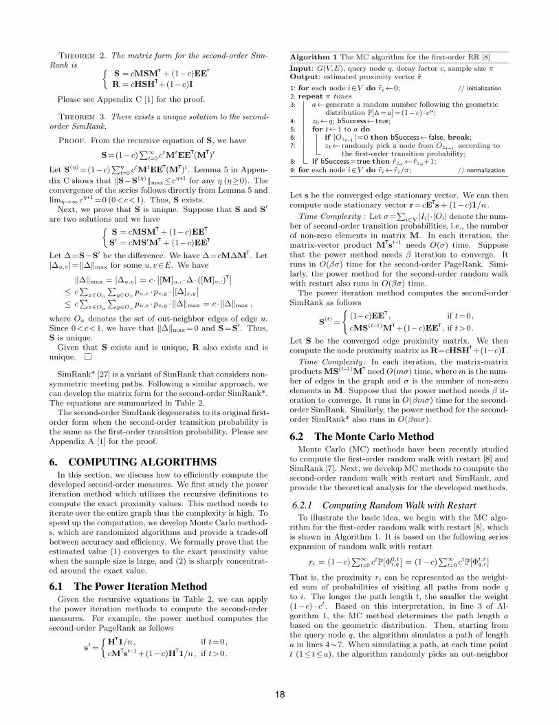
Algorithm 1 The MC algorithm for the first-order RR [8]

Input: G(V,E), query node q, decay factor c, sample size πOutput: estimated proximity vector r

1: for each node i∈V do ri←0; // initialization

2: repeat π times3: a←generate a random number following the geometric

distribution P[A=a]=(1−c) ·ca;4: z0←q; bSuccess← true;5: for t←1 to a do6: if |Ozt 1 |=0 then bSuccess← false, break;7: zt← randomly pick a node from Ozt 1 according to

the first-order transition probability;8: if bSuccess= true then rza← rza+1;9: for each node i∈V do ri← ri/π; // normalization

Let s be the converged edge stationary vector. We can thencompute node stationary vector r=cE s + (1−c)1/n .

Time Complexity : Let σ=∑i∈V |Ii|·|Oi| denote the num-

ber of second-order transition probabilities, i.e., the numberof non-zero elements in matrix M. In each iteration, thematrix-vector product M st 1 needs O(σ) time. Supposethat the power method needs β iteration to converge. Itruns in O(βσ) time for the second-order PageRank. Simi-larly, the power method for the second-order random walkwith restart also runs in O(βσ) time.

The power iteration method computes the second-orderSimRank as follows

S(t) =

{(1−c)EE , if t=0 ,

cMS(t 1)M +(1−c)EE , if t>0 .

Let S be the converged edge proximity matrix. We thencompute the node proximity matrix as R=cHSH +(1−c)I .

Time Complexity: In each iteration, the matrix-matrixproducts MS(t 1)M need O(mσ) time, where m is the num-ber of edges in the graph and σ is the number of non-zeroelements in M. Suppose that the power method needs β it-eration to converge. It runs in O(βmσ) time for the second-order SimRank. Similarly, the power method for the second-order SimRank* also runs in O(βmσ).

6.2 The Monte Carlo MethodMonte Carlo (MC) methods have been recently studied

to compute the first-order random walk with restart [8] andSimRank [7]. Next, we develop MC methods to compute thesecond-order random walk with restart and SimRank, andprovide the theoretical analysis for the developed methods.

6.2.1 Computing Random Walk with RestartTo illustrate the basic idea, we begin with the MC algo-

rithm for the first-order random walk with restart [8], whichis shown in Algorithm 1. It is based on the following seriesexpansion of random walk with restart

ri = (1−c)∑∞t 0 c

tP[Φ0,ti,q ] = (1−c)

∑∞t 0 c

tP[Φt,tq,i ]

That is, the proximity ri can be represented as the weight-ed sum of probabilities of visiting all paths from node qto i. The longer the path length t, the smaller the weight(1−c) · ct. Based on this interpretation, in line 3 of Al-gorithm 1, the MC method determines the path length abased on the geometric distribution. Then, starting fromthe query node q, the algorithm simulates a path of lengtha in lines 4∼7. When simulating a path, at each time pointt (1≤ t≤a), the algorithm randomly picks an out-neighbor

18

Algorithm 2 The MC algorithm for the second-order RR

Input: G(V,E), query node q, decay factor c, sample size πOutput: estimated proximity vector r

1: for each node i∈V do ri←0; // initialization

2: repeat π times3: a←generate a random number following the geometric

distribution P[A=a]=(1−c) ·ca;4: z0←q; bSuccess← true;5: for t←1 to a do6: if |Ozt 1 |=0 then bSuccess← false, break;7: if t=1 then zt← randomly pick a node from Ozt 1

according to the first-order transition probability;8: else zt←randomly pick a node from Ozt 1 according

to the second-order transition probability;9: if bSuccess= true then rza← rza+1;10:for each node i∈V do ri← ri/π; // normalization

of the previous node zt 1 to visit according to the first-ordertransition probability. The algorithm stops when the sim-ulated path reaches length a or there is no out-neighbor topick. The algorithm repeats this process π times, where π isthe number of paths to be simulated. The proximity valueof node i is estimated as the fraction of the π paths that endat i.

We can extend this MC algorithm to compute the second-order random walk with restart as shown in Algorithm 2. Itis based on the series expansion

ri = (1−c)∑∞t 0 c

tM[Φ0,ti,q ] = (1−c)

∑∞t 0 c

tM[Φt,tq,i ]

That is, the proximity ri can be represented as the weightedsum of probabilities of visiting all paths from node q to iin the second-order random walk. The difference betweenAlgorithm 1 and Algorithm 2 is how to sample a path. Inlines 5∼7 of Algorithm 1, at each step, the algorithm picksan out-neighbor with the first-order transition probability.In lines 5∼ 8 of Algorithm 2, only in the first step, i.e.,when t= 1, the algorithm picks an out-neighbor with thefirst-order transition probability. Then the algorithm picksout-neighbors with the second-order transition probabilitieswhen simulating subsequent steps.

Theorem 4 shows that when the sample size is large, theestimated proximity ri converges to the exact proximity ri.Theorem 5 shows that the error is bounded by a term thatis exponentially small in terms of the sample size.

Theorem 4. The estimated proximity ri converges to theexact proximity ri when π→∞.

Proof. In Algorithm 2, if we successfully sample a pathending at node i, we will increase ri by 1; otherwise, ri is

unchanged. Let S(d)i be a Bernoulli random variable denot-

ing the incremental value of ri at the d-th iteration (lines

3∼9). Random variables S(1)i , S(2)

i , · · · , S(π)i are independent

and identically distributed. Let Si be a Bernoulli random

variable following the same distribution as S(d)i ’s. Lemma 6

in Appendix D [1] shows that the expected value of Si equalsthe exact proximity ri, i.e., E[Si] = ri .

Let Si= 1π

∑πd 1 S

(d)i be the sample average, which repre-

sents the estimated proximity ri. By the law of large num-bers, if the sample size π→∞, Si converges to the expectedvalue E[Si] = ri .

Theorem 5. For any ε>0, we have that

P[|ri−ri|≥ε] ≤ 2 ·exp(−2πε2)

Algorithm 3 The basic MC algorithm for the first-order SR [7]

Input: G(V,E), query node q, decay factor c, sample size π,maximum length η

Output: estimated proximity vector r

1: for each node i∈V do // process each node individually

2: ri←0; // initialization

3: repeat π times // sample π pairs of paths

4: sample a path q= z0→z1→ ·· · →zη starting from q;5: sample a path i = z′0→z′1→ ·· · →z′η starting from i;

// find the common node with the smallest offset

6: for t= 0 to η do if zt= z′t then ri← ri+ ct, break;7: ri← ri/π; // normalization

Proof. Following the notations defined in the proof of

Theorem 4, random variables S(1)i ,S(2)

i , · · · ,S(π)i are indepen-

dent and bounded by interval [0,1]. By Hoeffding’s inequal-ity [10], we can prove this theorem.

Time Complexity : Generating a random number costsO(1) time. Since the path length a follows the geometric dis-tribution, the average length is (1− c)

∑∞a 0ac

a= c/(1− c).When sampling a path, at each step, the algorithm randomlypicks an out-neighbor, which costs O(ξ) on average, whereξ= 1

n

∑i∈V |Oi| denotes the average out-degree. Thus, on

average, sampling a path costs O(ξc/(1− c)) time. Sam-pling π paths costs O(πξc/(1−c)) time. Initialization andnormalization cost O(n) time. In total, Algorithm 2 runs inO(πξc/(1−c)+n) time.

The MC algorithm developed here is readily applicable tocompute the second-order PageRank. Let PR(i) denote thePageRank value of node i, and RRj(i) denote the randomwalk with restart proximity of node i when j is the query.

Theorem 6. PR(i) = 1n

∑j∈V RRj(i)

Proof. The proof is similar to that of the linearity theo-rem [12]. We omit the proof here due to the space limit.

Based on this theorem, we can use Algorithm 2 to computethe random walk with restart proximity vector for each node.The average of all vectors is the estimated PageRank vector.

6.2.2 Computing SimRankThe basic MC algorithm for computing the first-order

SimRank is proposed in [7], which is shown in Algorithm3. It is based on the original interpretation of SimRank[11], i.e., the proximity ri measures the expected number ofsteps required before two surfers, one starting at the querynode q and the other at node i, meet at the same node ifthey randomly walk on the reverse graph in lock-step.

As shown in Algorithm 3, the algorithm proposed in [7]directly simulates the meeting paths of the two surfers. Foreach node i, it simulates two paths of length η, one startingfrom node q and one from i. It then scans these two pathsto determine whether there is a common node. The fractionof the sampled paths that do have a common node is usedas the estimated proximity value for node i.

Algorithm 3 estimates the proximity of each node i indi-vidually and samples a fixed number of paths for each node.This method usually needs to simulate a large number ofmeeting paths to achieve an accurate estimation since notall simulated paths may have common nodes. The pathsthat do not have common nodes can only be used in thedenominator in the estimated proximity value.

19

Algorithm 4 The proposed MC algorithm for the first-order SR

Input: G(V,E), query node q, decay factor c, sample size π,maximum length η, matrix X

Output: estimated proximity vector r

1: for each node i∈V do ri←0; // initialization

2: repeat π times // sample π meeting paths

3: a←generate a random number following the geometricdistribution P[A=a]=(1−c) ·ca;

4: if a>η then continue;5: [bSuccess,z2a, δ]←SampleOneMeetingPath(q,a,X);

6: if bSuccess= true then rz2a← rz2a+δ;

7: for each node i∈V do ri← ri/π; // normalization

Algorithm 5 [bSuccess,z2a,δ]←SampleOneMeetingPath(q,a,X)

1: z0←q; bSuccess← true; // start from the query node

2: for t←1 to a do // sample the first half

3: if |Ozt 1 |=0 then bSuccess← false, return;

4: zt← randomly pick a node from Ozt 1 according to thefirst-order transition probability;

5: for t←(a+1) to 2a do // sample the second half

6: if |Izt 1|=0 or [X]zt 1,2a t 1=0 then bSuccess←false, return;

7: zt← randomly pick a node from Izt 1 according to the

probability pzt,zt 1 · [X]zt,2a t/[X]zt 1,2a t 1;

8: δ← [X]za,a/[X]z2a,0 ;

Algorithm 6 ComputeNodeVisitingProbabilities()

Input: G(V,E), transition matrix P, maximum length ηOutput: n×(η+1) matrix X

1: [X]:,0←1/n; // begin from the uniform probability distribution

2: for t←1 to η do [X]:,t←P [X]:,t 1;

Next, we propose a new sampling strategy to computethe SimRank values. Our sampling method estimates theproximity values for all the nodes at the same time. Everysimulated path is guaranteed to contribute to the numeratorof some node and to the denominators of all nodes. Experi-mental results show that compared to the previous method,our sampling method needs several orders of magnitude lesssimulated paths to achieve the same accuracy.

For simplicity, next, we illustrate the key idea of the de-veloped sampling strategy for the first-order SimRank. Itcan be easily extended to the second-order SimRank.

Algorithm 4 shows the overall procedure of the proposedalgorithm, which is based on the series expansion

ri = (1−c)∑∞t 0 c

tP[Φt,2ti,q ] = (1−c)∑∞t 0 c

tP[Φt,2tq,i ]

That is, the proximity ri can be represented as the weightedsum of probabilities of visiting all meeting paths of length{t,2t} between nodes q and i.

Instead of simulating meeting paths starting from bothnodes q and i, we only simulate paths starting from q. Algo-rithm 5 shows the procedure to sample a meeting path. Fora meeting path φ : q=z0→z1→·· ·→za←·· ·←z2a 1←z2a=i,when simulating the first half of the path, we simply followthe first-order transition probability. Since the second halfof the meeting path is in reverse order, we need to pick in-neighbors of the visited nodes. To do that, we need to knowthe probability of visiting in-neighbors. We can use Bayes’theorem to calculate these probabilities.

Let Xt be a random variable representing the node visitedby the surfer at time t. Suppose that node j is an in-neighborof k, i.e., j∈Ik. We have

P[Xt 1=j|Xt=k]=P[Xt 1=j]

P[Xt=k]·P[Xt=k|Xt 1=j]=

P[Xt 1=j]

P[Xt=k]·pj,k

Thus to calculate the probability of visiting in-neighbors,we only need the prior probability of visiting each node.Algorithm 6 computes these probabilities and stores themin an n× (η+1) matrix X in the preprocessing stage, with[X]j,t = P[Xt = j], where η is the maximum length of thesimulated paths.

Let ri = (1− c)∑ηt 0 c

tP[Φt,2tq,i ] be the SimRank value wetry to estimate. Next, we show that our sampling strategygives accurate estimation of ri .

Theorem 7. The estimated proximity ri converges to riwhen π→∞.

Proof. In Algorithm 4, if we successfully sample a pathending at node i, we will increase ri by δ; otherwise, ri isunchanged. For different sampled paths, the corresponding

value δ may be different. Let R(d)i be a random variable

denoting the incremental value of ri at the d-th iteration

(lines 3∼ 6). Random variables R(1)i ,R(2)

i , · · · ,R(π)i are in-

dependent and identically distributed. Let Ri be a random

variable following the same distribution as R(d)i ’s. Lemma

7 in Appendix D [1] shows that the expected value of Riequals the truncated proximity ri, i.e., E[Ri] = ri .

Let Ri= 1π

∑πd 1R

(d)i be the sample average, which repre-

sents the estimated proximity ri. By the law of large num-bers, if the sample size π→∞, Ri converges to the expectedvalue E[Ri] = ri .

Theorem 8. For any ε>0, we have that

P[ri−ri≤−ε]≤exp(−πε2

2nri) and P[ri−ri≥ε]≤exp( −πε2

2nri+2nε/3).

Proof. Following the notations defined in the proof of

Theorem 7, random variables R(1)i ,R(2)

i , · · · ,R(π)i are inde-

pendent and bounded by interval [0, δ] ⊆ [0,n]. Lemma 7in Appendix D [1] shows that the expected value of R2

i isbounded from above by nri , i.e., E[R2

i ]≤nri . Thus, we have

that∑πd 1E[(R(d)

i )2]≤πnri . By Theorem 14 in AppendixD [1], we can prove this theorem.

Time Complexity : Since the path length a follows the ge-ometric distribution, the average length is (1−c)

∑∞a 0 2aca=

2c/(1− c). When sampling a path in Algorithm 5, at eachstep, the algorithm randomly picks an out-neighbor or in-neighbor, which costs O(ψ) time on average, where ψ =1

2n

∑i∈V(|Ii| + |Oi|

)denotes the average degree. Thus, on

average, sampling a path costs O(ψc/(1− c)). Sampling πpaths costs O(πψc/(1−c)). Initialization and normalizationcost O(n). In total, Algorithm 4 runs in O(πψc/(1−c)+n)time. Algorithm 6 runs in O(mη) time.

The proposed MC algorithm is readily applicable to thesecond-order SimRank. The only difference is that in thesecond-order SimRank, we need to follow the second-ordertransition probability when sampling meeting paths. The-orems 7 and 8 also apply when we follow the second-ordertransition probability.

7. EXPERIMENTAL RESULTSIn this section, we perform comprehensive experimental

evaluations on the developed methods. To evaluate the effec-tiveness of the developed second-order proximity measures,

20

Figure 6: Ranking accuracy Figure 7: Query accuracy

we use both networks with and without the data flow infor-mation. We also evaluate the efficiency of proposed com-puting methods on large real and synthetic networks.

All programs are written in C++, and all experiments areperformed on a server with 32G memory, Intel Xeon 3.2GHzCPU, and Redhat OS.

7.1 Networks with Data Flow InformationWe first evaluate the effectiveness of the second-order mea-

sures using networks with data flow information.

7.1.1 Web Domain Network with Clickstream DataIn the web domain network, each node represents a do-

main, and an edge is weighted by the number of hyperlinksbetween pages contained in the two connected domains. Theweb graph was gathered in 2012 and is publicly available athttp://webdatacommons.org/hyperlinkgraph/ [17]. It contains463,824 domains and 6,285,354 edges.

Clickstream data records the sequences of domains visitedby different users [3]. The clickstream data is obtained fromcomScore Inc. It contains 5,000 users’ clickstreams recordedover 6 months in 2012. The total number of visits is 62.4million. Each domain was visited 135 times on average.

We first evaluate the domain ranking results of PageRank(PR). The original first-order PR [22], multilinear PR [9],memory PR [24], and our second-order PR (PR2) are usedfor comparison. PR uses the first-order transition probabil-ity. Multilinear PR approximates the stationary probabilityof an edge by the product of stationary probabilities of itstwo end nodes. Memory PR and PR2 use the second-ordertransition probabilities based on the frequencies of the tri-grams in the clickstream data as discussed in Section 3.3.

We use Alexa’s top domains (http://alexa.com/topsites)as the reference to evaluate the ranking results of the select-ed measures. The Normalized Discounted Cumulative Gain(NDCG) is used as the evaluation metric [27]. The NDCG

value at position k is NDCGk=β∑ki 1(2

s(i)−1)/ log2(1+ i),where s(i) is the score of the i-th node and β is a normal-izing factor to ensure the NDCG value of the ground-truthordering to be 1. We use NDCG100 to evaluate the top-100ranked domains of the selected measures. A retrieved do-main gets a score of 1 if it appears in the top-100 domainsin Alexa’s top domains; otherwise, it gets a score of 0.

In addition to using Alexa’s top domains as the reference,we also hired 10 human evaluators to manually evaluate theretrieved domains. An evaluator gives an importance score(ranging from 1 to 5, with 5 being the most important) toeach retrieved domain. For each domain, the average scoreof all evaluators is used as its final score. NDCG100 is thencalculated as the evaluation metric.

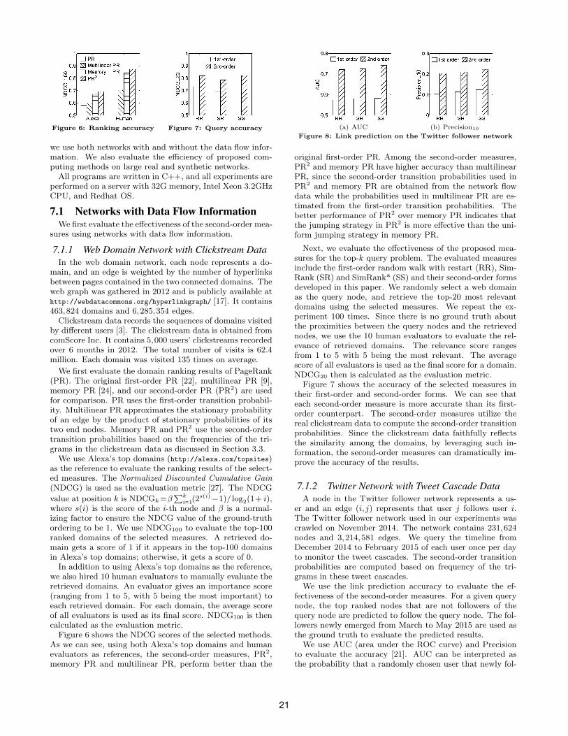
Figure 6 shows the NDCG scores of the selected methods.As we can see, using both Alexa’s top domains and humanevaluators as references, the second-order measures, PR2,memory PR and multilinear PR, perform better than the

(a) AUC (b) Precision10

Figure 8: Link prediction on the Twitter follower network

original first-order PR. Among the second-order measures,PR2 and memory PR have higher accuracy than multilinearPR, since the second-order transition probabilities used inPR2 and memory PR are obtained from the network flowdata while the probabilities used in multilinear PR are es-timated from the first-order transition probabilities. Thebetter performance of PR2 over memory PR indicates thatthe jumping strategy in PR2 is more effective than the uni-form jumping strategy in memory PR.

Next, we evaluate the effectiveness of the proposed mea-sures for the top-k query problem. The evaluated measuresinclude the first-order random walk with restart (RR), Sim-Rank (SR) and SimRank* (SS) and their second-order formsdeveloped in this paper. We randomly select a web domainas the query node, and retrieve the top-20 most relevantdomains using the selected measures. We repeat the ex-periment 100 times. Since there is no ground truth aboutthe proximities between the query nodes and the retrievednodes, we use the 10 human evaluators to evaluate the rel-evance of retrieved domains. The relevance score rangesfrom 1 to 5 with 5 being the most relevant. The averagescore of all evaluators is used as the final score for a domain.NDCG20 then is calculated as the evaluation metric.

Figure 7 shows the accuracy of the selected measures intheir first-order and second-order forms. We can see thateach second-order measure is more accurate than its first-order counterpart. The second-order measures utilize thereal clickstream data to compute the second-order transitionprobabilities. Since the clickstream data faithfully reflectsthe similarity among the domains, by leveraging such in-formation, the second-order measures can dramatically im-prove the accuracy of the results.

7.1.2 Twitter Network with Tweet Cascade DataA node in the Twitter follower network represents a us-

er and an edge (i, j) represents that user j follows user i.The Twitter follower network used in our experiments wascrawled on November 2014. The network contains 231,624nodes and 3,214,581 edges. We query the timeline fromDecember 2014 to February 2015 of each user once per dayto monitor the tweet cascades. The second-order transitionprobabilities are computed based on frequency of the tri-grams in these tweet cascades.

We use the link prediction accuracy to evaluate the ef-fectiveness of the second-order measures. For a given querynode, the top ranked nodes that are not followers of thequery node are predicted to follow the query node. The fol-lowers newly emerged from March to May 2015 are used asthe ground truth to evaluate the predicted results.

We use AUC (area under the ROC curve) and Precisionto evaluate the accuracy [21]. AUC can be interpreted asthe probability that a randomly chosen user that newly fol-

21

lows the query node is given a higher score than a randomlychosen user that does not follow the query node. Precisionis defined as Precisionk=k′/k, where k is the total numberof predicted users, and k′ is the number of users that actu-ally started to follow the query node. We randomly pick 103

query nodes and report the average.Figure 8(a) shows the AUC values of the first-order and

second-order RR, SR, and SS. We can observe that thesecond-order measures improve the AUC values by 23 ∼28% compared to their first-order counterparts. Figure 8(b)shows the Precision10 values. Similarly, the second-ordermeasures outperform the first-order measures consistently.The real tweet cascade data reflects how tweets propagateamong different users and provides more accurate transi-tion information than the network topology alone does. Thesecond-order measures use such information thus have bet-ter performance.

7.2 Networks without Data Flow InformationWhen the network data flow information is not avail-

able, we use three different applications, including local com-munity detection, link prediction, and graph-based semi-supervised learning, to evaluate the effectiveness of the de-veloped second-order proximity measures. We use the au-toregressive model discussed in Section 3.3 to obtain thesecond-order transition probabilities.

7.2.1 Local Community DetectionThe goal of local community detection is to find the com-

munity near a given query node [2, 26]. Intuitively, theidentified local community should contain the nodes havinglarge proximity to the query node. We use the query bi-ased densest connected subgraph (QB) method [26] and thePageRank-Nibble (NB) method [2] to evaluate the developedsecond-order measure. For a given query node, both QB andNB compute the node proximity values and use them to finda set of top-ranked nodes as the identified local community.Both methods use the first-order random walk with restart(RR) as their proximity measure. We simply replace thefirst-order RR with the proposed second-order RR (RR2)in QB and NB. All other parts in QB and NB remain thesame as the original algorithms. The second-order transi-tion probability is computed by the autoregressive modeland the default setting for α is 0.2.

We use F-score and consistency [26] as the evaluation met-rics. F-score measures the accuracy of the detected com-munity with regard to the ground-truth community labels.Consistency measures the standard deviation of F-scores ofthe identified communities when different nodes in the samecommunity are used as the query nodes. A high consistencyvalue indicates that the method tends to find the same localcommunity no matter which node in it is used as the query.We randomly pick 103 query nodes and report the average.

We first use real networks to evaluate the performance ofthe second-order measure. Table 3 shows the statistics ofreal networks. These datasets are provided with ground-truth community memberships and are publicly available athttp://snap.stanford.edu.

Figure 9(a) shows the F-scores on these networks. QBwith RR2 outperforms QB with RR for 26∼44%. NB withRR2 outperforms NB with RR for 18∼62%. Using RR2, therandom surfer is more likely to be trapped within the local

Table 3: Statistics of real networks

datasets abbr. #nodes #edges #communities

Amazon AZ 334,863 925,872 151,037

DBLP DP 317,080 1,049,866 13,477

Youtube YT 1,134,890 2,987,624 8,385

LiveJournal LJ 3,997,962 34,681,189 287,512

(a) F-score (b) consistency

Figure 9: F-scores and consistency values on real networks

(a) the QB method (b) the NB method

Figure 10: Tuning the parameter α (Amazon network, RR2)

(a) the QB method (b) the NB method

Figure 11: F-scores on synthetic networks

community containing the query node, since it takes the pre-vious step of the surfer into consideration. This results thatthe nodes in the local community have larger proximity val-ues than the nodes outside the community. It helps improvethe accuracy of the local community detection methods.

Figure 9(b) shows the consistency results. QB with RR2

outperforms QB with RR for 3∼ 11%. NB with RR2 out-performs NB with RR for 8∼15%. High consistency is im-portant for local community detection, since the identifiedcommunities should be similar even if different nodes in thesame community are used as the query. The higher consis-tency value of RR2 demonstrates that it better captures thecommunity structures.

Next we evaluate the sensitivity of RR2 with respect tothe tuning parameter α. Figure 10(a) shows the F-scores ofQB with RR2 on the Amazon network for different α values.We can see that the performance is stable when varying α.When α=0.2, QB has the best performance. Figure 10(b)shows the results of NB with RR2. A similar trend can beobserved. Note that when α= 0, RR2 degenerates to RRand has the same performance as RR.

In addition to real networks, we also generate a collectionof synthetic networks using the graph generator in [14] toevaluate the developed second-order measures. The numberof nodes in the network is 220 and the number of edges is 107.The network generating model contains a mixing parameterµ, which indicates the proportion of a node’s neighbors thatreside in other communities. By tuning µ, we can vary the

22

Figure 12: Link prediction on theco-author network

Figure 13: Graph-basedsemi-supervised learning

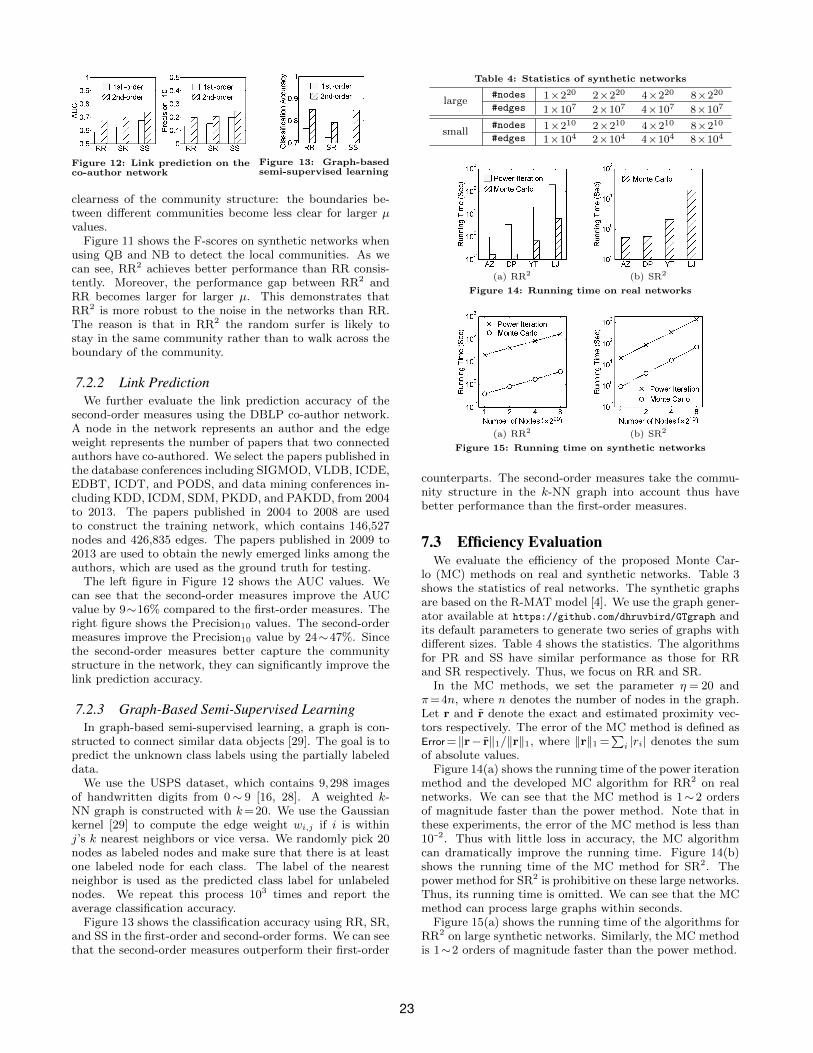
clearness of the community structure: the boundaries be-tween different communities become less clear for larger µvalues.

Figure 11 shows the F-scores on synthetic networks whenusing QB and NB to detect the local communities. As wecan see, RR2 achieves better performance than RR consis-tently. Moreover, the performance gap between RR2 andRR becomes larger for larger µ. This demonstrates thatRR2 is more robust to the noise in the networks than RR.The reason is that in RR2 the random surfer is likely tostay in the same community rather than to walk across theboundary of the community.

7.2.2 Link PredictionWe further evaluate the link prediction accuracy of the

second-order measures using the DBLP co-author network.A node in the network represents an author and the edgeweight represents the number of papers that two connectedauthors have co-authored. We select the papers published inthe database conferences including SIGMOD, VLDB, ICDE,EDBT, ICDT, and PODS, and data mining conferences in-cluding KDD, ICDM, SDM, PKDD, and PAKDD, from 2004to 2013. The papers published in 2004 to 2008 are usedto construct the training network, which contains 146,527nodes and 426,835 edges. The papers published in 2009 to2013 are used to obtain the newly emerged links among theauthors, which are used as the ground truth for testing.

The left figure in Figure 12 shows the AUC values. Wecan see that the second-order measures improve the AUCvalue by 9∼16% compared to the first-order measures. Theright figure shows the Precision10 values. The second-ordermeasures improve the Precision10 value by 24∼47%. Sincethe second-order measures better capture the communitystructure in the network, they can significantly improve thelink prediction accuracy.

7.2.3 Graph-Based Semi-Supervised LearningIn graph-based semi-supervised learning, a graph is con-

structed to connect similar data objects [29]. The goal is topredict the unknown class labels using the partially labeleddata.

We use the USPS dataset, which contains 9,298 imagesof handwritten digits from 0∼ 9 [16, 28]. A weighted k-NN graph is constructed with k=20. We use the Gaussiankernel [29] to compute the edge weight wi,j if i is withinj’s k nearest neighbors or vice versa. We randomly pick 20nodes as labeled nodes and make sure that there is at leastone labeled node for each class. The label of the nearestneighbor is used as the predicted class label for unlabelednodes. We repeat this process 103 times and report theaverage classification accuracy.

Figure 13 shows the classification accuracy using RR, SR,and SS in the first-order and second-order forms. We can seethat the second-order measures outperform their first-order

Table 4: Statistics of synthetic networks

large#nodes 1×220 2×220 4×220 8×220

#edges 1×107 2×107 4×107 8×107

small#nodes 1×210 2×210 4×210 8×210

#edges 1×104 2×104 4×104 8×104

(a) RR2 (b) SR2

Figure 14: Running time on real networks

(a) RR2 (b) SR2

Figure 15: Running time on synthetic networks

counterparts. The second-order measures take the commu-nity structure in the k-NN graph into account thus havebetter performance than the first-order measures.

7.3 Efficiency EvaluationWe evaluate the efficiency of the proposed Monte Car-

lo (MC) methods on real and synthetic networks. Table 3shows the statistics of real networks. The synthetic graphsare based on the R-MAT model [4]. We use the graph gener-ator available at https://github.com/dhruvbird/GTgraph andits default parameters to generate two series of graphs withdifferent sizes. Table 4 shows the statistics. The algorithmsfor PR and SS have similar performance as those for RRand SR respectively. Thus, we focus on RR and SR.

In the MC methods, we set the parameter η = 20 andπ=4n, where n denotes the number of nodes in the graph.Let r and r denote the exact and estimated proximity vec-tors respectively. The error of the MC method is defined asError =‖r− r‖1/‖r‖1, where ‖r‖1 =

∑i |ri| denotes the sum

of absolute values.Figure 14(a) shows the running time of the power iteration

method and the developed MC algorithm for RR2 on realnetworks. We can see that the MC method is 1∼2 ordersof magnitude faster than the power method. Note that inthese experiments, the error of the MC method is less than10 2. Thus with little loss in accuracy, the MC algorithmcan dramatically improve the running time. Figure 14(b)shows the running time of the MC method for SR2. Thepower method for SR2 is prohibitive on these large networks.Thus, its running time is omitted. We can see that the MCmethod can process large graphs within seconds.

Figure 15(a) shows the running time of the algorithms forRR2 on large synthetic networks. Similarly, the MC methodis 1∼2 orders of magnitude faster than the power method.

23

(a) real network, LiveJournal (b) synthetic network, 220 nodes

Figure 16: Error versus running time (first-order SimRank)

The power method for SR2 is prohibitive on large net-works, thus we report the results on small networks. Notethat the proposed MC method is applicable on large net-works. Since the power method computes all-pairs proxim-ity, to compare with the power method, we use each nodeas the query node and call the MC method. In this way, wealso compute all-pairs proximity using the MC method. Wethen report the overall running time. Figure 15(b) showsthe running time on synthetic networks. We can see thatthe MC method is 1∼2 orders of magnitude faster than thepower method. The error of the MC method is also less than10 2 in all these experiments.

We further compare the sampling strategy in the MCmethod developed in [7] and our sampling strategy describedin Algorithm 5. Recall that the method in [7] samples meet-ing paths starting from the query node q and every othernode i, while our method samples the meeting paths allstarting from the query node. We compare the running timethat the two methods need to take to achieve the same ac-curacy. When varying the number of sampled paths, therunning time and accuracy of the two methods will changecorrespondingly. For each setting, we repeat the query 103

times with randomly picked query nodes and report the av-erage running time and error.

Figure 16(a) shows the error versus running time on theLiveJournal network. We can see that to achieve the sameaccuracy, the proposed method is about 3 orders of magni-tude faster than the previous method. This demonstratesthe advantage of the proposed sampling strategy. Figure16(b) shows the error versus running time on the syntheticgraph with 220 nodes. A similar trend can be observed.

8. CONCLUSIONSDesigning effective proximity measures for large graphs

is an important and challenging task. Most existing ran-dom walk based measures only use the first-order transitionprobability. In this paper, we investigate the second-orderrandom walk measures which can capture the cluster struc-tures in the graph and better model real-life applications.We provide rigorous theoretical foundations for the second-order random walk and develop second-order forms for com-monly used measures. We further develop effective MonteCarlo methods to compute these measures. Extensive exper-imental results demonstrate that the second-order measurescan effectively improve the accuracy in various applications,and the developed Monte Carlo methods can significantlyspeed up the computation with little loss in accuracy.

Acknowledgements. This work was partially supportedby the National Science Foundation grants IIS-1162374, CA-REER, and the NIH grant R01GM115833.

9. REFERENCES[1] http://www.robwu.net .[2] R. Andersen, F. Chung, and K. Lang. Local graph partition-

ing using PageRank vectors. In FOCS, pp. 475–486, 2006.[3] R. E. Bucklin and C. Sismeiro. Click here for internet insight:

Advances in clickstream data analysis in marketing. Journalof Interactive Marketing, 23(1):35–48, 2009.

[4] D. Chakrabarti, Y. Zhan, and C. Faloutsos. R-MAT: A recur-sive model for graph mining. In SDM, pages 442–446, 2004.

[5] F. Chung and L. Lu. Complex graphs and networks, chapterOld and new concentration inequalities. AMS, 2006.

[6] S. Cohen, B. Kimelfeld, and G. Koutrika. A survey on prox-imity measures for social networks. In Search Computing,pages 191–206, 2012.

[7] D. Fogaras and B. Racz. Scaling link-based similarity search.In WWW, pages 641–650, 2005.

[8] D. Fogaras, B. Racz, K. Csalogany, et al. Towards scalingfully personalized PageRank: Algorithms, lower bounds, andexperiments. Internet Mathematics, 2(3):333–358, 2005.

[9] D. F. Gleich, L.-H. Lim, and Y. Yu. Multilinear PageRank.SIAM Journal on Matrix Analysis and Applications, 2015.

[10] W. Hoeffding. Probability inequalities for sums of boundedrandom variables. JASA, 58(301):13–30, 1963.

[11] G. Jeh and J. Widom. SimRank: A measure of structural-context similarity. In KDD, pages 538–543, 2002.

[12] G. Jeh and J. Widom. Scaling personalized web search. InWWW, pages 271–279, 2003.

[13] M. Kusumoto, T. Maehara, and K. Kawarabayashi. Scalablesimilarity search for SimRank. InSIGMOD, pp.325-336,2014.

[14] A. Lancichinetti, S. Fortunato, and F. Radicchi. Benchmarkgraphs for testing community detection algorithms. PhysicalReview E, 78(4):046110, 2008.

[15] A. N. Langville and C. D. Meyer. Google’s PageRank andbeyond: The science of search engine rankings, chapter Themathematics guide. Princeton University Press, 2006.

[16] Y. LeCun, B. E. Boser, et al. Handwritten digit recognitionwith a back-propagation network. In NIPS, 1990.

[17] O. Lehmberg, R. Meusel, and C. Bizer. Graph structure inthe web: Aggregated by pay-level domain. In WebSci, pages119–128, 2014.

[18] C. Li, J. Han, G. He, X. Jin, Y. Sun, Y. Yu, and T. Wu. Fastcomputation of SimRank for static and dynamic informationnetworks. In EDBT, pages 465–476, 2010.

[19] D. Liben-Nowell and J. Kleinberg. The link-prediction prob-lem for social networks. JASIST, 58(7):1019–1031, 2007.

[20] S. Lim, S. Ryu, S. Kwon, K. Jung, and J.-G. Lee.LinkSCAN*: Overlapping community detection using thelink-space transformation. In ICDE, pages 292–303, 2014.

[21] L. Lu and T. Zhou. Link prediction in complex networks: Asurvey. Physica A, 390(6):1150–1170, 2011.

[22] L. Page, S. Brin, R. Motwani, and T. Winograd. The PageR-ank citation ranking: Bringing order to the web. 1999.

[23] A. E. Raftery. A model for high-order Markov chains. J. ofthe Royal Statistical Society: Series B, pages 528–539, 1985.

[24] M. Rosvall, A. V. Esquivel, A. Lancichinetti, et al. Memoryin network flows and its effects on spreading dynamics andcommunity detection. Nature Commun., 5(4630), 2014.

[25] H. Tong, C. Faloutsos, and J.-Y. Pan. Fast random walk withrestart and its applications. In ICDM, pages 613–622, 2006.

[26] Y. Wu, R. Jin, J. Li, and X. Zhang. Robust local communitydetection: On free rider effect and its elimination. PVLDB,8(7):798–809, 2015.

[27] W. Yu, X. Lin, W. Zhang, L. Chang, and J. Pei. More issimpler: Effectively and efficiently assessing node-pair simi-larities based on hyperlinks. PVLDB, 7(1):13–24, 2013.

[28] X. Zhu, Z. Ghahramani, and J. Lafferty. Semi-supervisedlearning using Gaussian fields and harmonic functions. InICML, pages 912–919, 2003.

[29] X. Zhu and A. Goldberg. Introduction to semi-supervisedlearning, chapter Graph-based semi-supervised learning.Morgan & Claypool Publishers, 2009.

24