PNNL-14152

Remote Chemical Sensing Using Quantum Cascade Lasers WW Harper JR Schultz December 2002 Prepared for the U.S. Department of Energy under Contract DE-AC06-76RL01830

DISCLAIMER

This report was prepared as an account of work sponsored by an agency of the United States Government. Neither the United States Government nor any agency thereof, nor Battelle Memorial Institute, nor any of their employees, makes any warranty, express or implied, or assumes any legal liability or responsibility for the accuracy, completeness, or usefulness of any information, apparatus, product, or process disclosed, or represents that its use would not infringe privately owned rights. Reference herein to any specific commercial product, process, or service by trade name, trademark, manufacturer, or otherwise does not necessarily constitute or imply its endorsement, recommendation, or favoring by the United States Government or any agency thereof, or Battelle Memorial Institute. The views and opinions of authors expressed herein do not necessarily state or reflect those of the United States Government or any agency thereof.

PACIFIC NORTHWEST NATIONAL LABORATORY operated by BATTELLE

for the UNITED STATES DEPARTMENT OF ENERGY

under Contract DE-AC06-76RL01830

Printed in the United States of America

Available to DOE and DOE contractors from the Office of Scientific and Technical Information,

P.O. Box 62, Oak Ridge, TN 37831-0062; ph: (865) 576-8401 fax: (865) 576-5728

email: reports@adonis.osti.gov

Available to the public from the National Technical Information Service, U.S. Department of Commerce, 5285 Port Royal Rd., Springfield, VA 22161

ph: (800) 553-6847 fax: (703) 605-6900

email: orders@ntis.fedworld.gov online ordering: http://www.ntis.gov/ordering.htm

This document was printed on recycled paper. (8/00)

PNNL-14152

Remote Chemical Sensing Using Quantum Cascade Lasers Warren W. Harper John F. Schultz December 2002 Prepared for the U.S. Department of Energy under Contract DE-AC06-76RL01830 Pacific Northwest National Laboratory Richland, Washington 99352

iii

Contents 1.0 Introduction and Summary ................................................................................................ 1 1.1 Background .............................................................................................................. 1 1.2 Summary of FM DIAL Work Performed in FY02........................................................ 2 2.0 FM DIAL System Description and Characterization ............................................................ 2 2.1 FM Lidar Transmitter/Source Characterization ............................................................ 5 2.1.1 Laser Beam Divergence................................................................................... 5 2.1.2 Laser Frequency Calibration ............................................................................ 7 2.1.3 QC Laser Modulation Properties ...................................................................... 9 2.2 FM DIAL Receiver/Detector Characterization............................................................. 12 2.2.1 Receiver Noise and Response .......................................................................... 13 2.2.2 Detector/Preamp Linearity ............................................................................... 16 3.0 FM DIAL Experiments ..................................................................................................... 17 3.1 Monostatic Experiments ............................................................................................ 18 3.2 Bistatic ..................................................................................................................... 20 3.3 Perimeter Monitoring ................................................................................................ 21 4.0 Detection/Data Processing Development ............................................................................ 23 4.1 Intensity Noise Mitigation.......................................................................................... 24 4.2 Quantitative Signal Verification ................................................................................. 26 5.0 Future Plans ..................................................................................................................... 28 6.0 References ...................................................................................................................... 29

iv

Figures 2.1 Experimental Setup for FY01 (left) and FY02 (right) .......................................................... 3 2.2 Cart Optical Layout ......................................................................................................... 4 2.3 QC Laser Dewar and 5-Axis Lens Mount ........................................................................... 6 2.4 Laser Spot at 46 m, the Scale on the Ruler is Graduated in 1-cm Increments......................... 6 2.5 Laser Windows that are Accessible with the QC Laser Used in This Work ........................... 8 2.6 Laser Wavenumber Windows as a Function of Drive Current .............................................. 8 2.7 The Detector Response to the RAM of a QC Laser is Shown as a Function of Frequency and Current.................................................................................................. 10 2.8 The Modulation Index Due to a Current Modulation (dν/di) is Shown as a Function of Current and Modulation Frequency .................................................... 11 2.9 Frequency Modulation Index (dν/di) Plotted on a Semi-Log Plot ................................ 12 2.10 RAM and FM Detection Phase .......................................................................................... 12 2.11 Noise Density for the Detector/Preamp Combination Used for FY02.................................... 14 2.12 Detector/Preamp Linearity Curve ....................................................................................... 16 3.1 Experimental Configurations Used with the FM Lidar System............................................. 17 3.2 Preliminary Monostatic Field Experiment Test ................................................................... 19 3.3 Experimental Data Collected During Field Experiments from a 40 m Monostatic Experiment ..................................................................................................... 19 3.4 Bistatic Experiment over a Range of 1.0 km One-Way........................................................ 21 3.5 Perimeter Monitoring Configuration Used to Detect a Nitrous Oxide Chemical Release........ 22 4.1 Noise Reduction Demonstration......................................................................................... 25 4.2 Agreement Between the Absorption Calculated from the Added N2O Pressure and the Observed Direct Absorption Signal........................................................................ 27 4.3 Agreement Between the Observed Lock-in Detection Results and the Signal Calculated from the Direct Absorption Experiment ................................................... 27

v

Table 2.1 FM Lidar Specifications .................................................................................................... 3

1

1.0 Introduction and Summary

1.1 Background Spectroscopic chemical sensing research at Pacific Northwest National Laboratory (PNNL) is focused on developing advanced sensors for detecting the production of nuclear, chemical, or biological weapons; use of chemical weapons; or the presence of explosives, firearms, narcotics, or other contraband of significance to homeland security in airports, cargo terminals, public buildings, or other sensitive locations. For most of these missions, the signature chemicals are expected to occur in very low concentrations, and in mixture with ambient air or airborne waste streams that contain large numbers of other species that may interfere with spectroscopic detection, or be mistaken for signatures of illicit activity. PNNL’s emphasis is therefore on developing remote and sampling sensors with extreme sensitivity, and resistance to interferents, or selectivity. PNNL’s research activities include: 1. Identification of signature chemicals and quantification of their spectral characteristics, 2. Identification and development of laser and other technologies that enable breakthroughs in

sensitivity and selectivity, 3. Development of promising sensing techniques through experimentation and modeling the

physical phenomenology and practical engineering limitations affecting their performance, and 4. Development and testing of data collection methods and analysis algorithms. Close coordination of all aspects of the research is important to ensure that all parts are focused on productive avenues of investigation. Close coordination of experimental development and numerical modeling is particularly important because the theoretical component provides understanding and predictive capability, while the experiments validate calculations and ensure that all phenomena and engineering limitations are considered. The spectroscopic chemical sensors being developed at PNNL fall into two categories: (1) remote sensors that interrogate the chemical content of air external to the sensor and (2) point sensors that draw air samples into the sensor for interrogation. Remote sensors offer the potential advantages of wide area coverage, covert detection, and standoff detection. However, "pressure broadening" of molecular spectra inevitably reduces the selectivity of remote sensors, and their sensitivity is limited by a wide array of phenomena that reduce signal levels and introduce noise. During the past decade, the Department of Energy's National Nuclear Security Administration/Nonproliferation Research and Engineering Office (DOE/NNSA/NA-22) has thoroughly investigated the phenomenology, engineering constraints, sensitivity, and selectivity of chemical sensors based on conventional differential absorption lidar (DIAL), passive Fourier transform spectrometers, and passive dispersive spectrometers. However, the unique tuning characteristics of quantum cascade lasers in any part of the mid-infrared spectral region (MWIR - wavelengths of 3 to 20 microns) combined with their small physical size, intrinsic robustness, excellent modulation and stability characteristics, and relatively high continuous-wave power levels enable new

2

remote sensing techniques that promise improved selectivity and sensitivity. PNNL is therefore developing frequency modula ted differential absorption lidar (FM DIAL) for a subset of the applications mentioned above where remote sensing is advantageous. FM DIAL has been described in detail previously (Sheen 2000; Schultz 2002). Quantum cascade lasers and some of the more recently available short-wave infrared lasers developed for telecommunications also enable a variety of novel point sensing techniques. PNNL is therefore developing novel point sensing techniques for applications that require extreme sensitivity and selectivity, and permit air sampling. This report describes the progress made on FM DIAL development in FY02.

1.2 Summary of FM DIAL Work Performed in FY02 During FY02, PNNL continued the development and characterization of an experimental FM DIAL system, initiated field chemical sensing experiments, and compared the results of experiments with numerical modeling results. In FY00 PNNL initiated systematic investigation of FM DIAL through development of a numerical model (Sheen 2000). In FY01 the investigation proceeded to construction of a laboratory-bench lidar (Cannon et al. 2001), and a series of exploratory experiments. In FY02 the FM DIAL system was mounted on a cart so that it could be wheeled outdoors and used for measurements and experiments requiring longer ranges than are available in our laboratory. Quantum cascade (QC) lasers and application of FM spectroscopy to remote sensing are both fairly novel, so little information relevant to component performance, the phenomenology of FM DIAL measurements, or data collection and analysis methods is available in the literature. PNNL's experimental research included systematic measurements of each component's performance characteristics. Various components were upgraded as possibilities for improvement became evident. Field experiments were conducted in three configurations of potential operational interest to identify the physical phenomena impacting range, sensitivity, and selectivity, and provide preliminary indications of potential performance and the limiting factors. Novel data collection and data analysis methods were developed to reduce noise and improve estimates of chemical concentrations.

2.0 FM DIAL System Description and Characterization Figure 2.1 depicts PNNL's FM DIAL system as it was originally assembled in FY01, and after it was mounted on a cart in FY02. The system is composed of a transmitter, receiver telescope, detector, and detection electronics. Key specifications for the system and its components are summarized in Table 2.1. The transmitter source is a QC laser that produces up to 100 mW of continuous wave (cw) power at wavelengths near 8.2 µm. (The laser's wavelength is often expressed as a "wavenumber," which is the number of waves in its optical field per centimeter, or cm-1. For a wavelength of 8.2 microns, the wavenumber is 1219 cm-1. One can also refer to the laser's optical frequency, which is the number of cycles of the electrical field per second. For a wavelength of 8.2 µm, the laser's optical frequency is 3.7×1013 Hz, or 37 THz. When the laser is frequency modulated, its optical frequency is slewed back and forth between maximum and minimum values at a specified "modulation frequency" (ωm) which is much lower than the optical frequency (ω0).

3

Figure 2.1. Experimental Setup for FY01 (left) and FY02 (right)

Table 2.1. FM Lidar Specifications

Configuration Mobile cart Receiver telescope diameter 25.4 cm (10”) Receiver telescope focal length 76.2 cm (30”) Detector diameter 1 mm Detector/preamp noise floor 2.4 pA/(Hz)1/2

Blackbody noise 3.0 pA/(Hz)1/2

Receiver field of view (FOV) 1.3 mrad Detection bandwidth 0.05 - 25 kHz QC laser power ≤100 mW QC laser wavelength 8.2 µm QC laser divergence 1.6 mrad Typical QC laser modulation frequency 200 kHz Typical QC laser optical scan range 1.5 cm-1 Typical QC laser modulation index ≤0.2 cm-1

The "modulation index" (M) is half of the difference between the maximum and minimum optical frequencies produced while the laser frequency is slewed. The instantaneous frequency (ωi) is given by:

( )tM mi ωωω sin0 += , where ω0 is the center frequency, M is the modulation index, and ωm is the modulation frequency. Modulation index can also be described in terms of wavenumbers, or cm-1. The laser wavelength can be

4

tuned over a range of 1.5 cm-1 by changing the electrical current used to drive it. The laser can also be tuned over a range of about 10 cm-1 by changing its operating temperature. Modulating the drive current can modulate the laser’s optical frequency. The modulation index achieved is a function of the frequency and amplitude of the current modulation. During FY02 we achieved modulation indices of about 2.25 GHz, or 0.075 cm-1, with typical current modulation frequencies of 200 kHz, and current modulation amplitudes of 20 mArms imposed on a DC drive current of 300 mA to 800 mA delivered at a compliance voltage of 6 V. The laser's output beam is focused to a divergence of 1.6 mrad with a pair of ZnSe lenses that have a focal length of 5.4 mm. The laser is then directed to the target with flat turning mirrors. Returning light is captured by an f3 all-reflective telescope with a primary mirror diameter of 10 inches, and imaged onto a mercury-cadmium-telluride (MCT) detector. After amplification, lock-in detection is used to recover signals at the modulation frequency with narrow bandwidth recovery. Signals from the lock-in amplifier are recorded by a digital storage oscilloscope, which allows additional averaging capabilities. Small amounts of light are split from the transmitted beam and directed to a reference cell containing a known gas, and to a reference etalon. The etalon provides frequency calibration and allows various QC laser properties to be measured. The reference cell can be used to lock the laser to a specific wavelength corresponding to a well-characterized absorption feature of the reference gas to permit precise, concurrent control of the wavelengths used for remote sensing. The reference cell also provides a known concentration of the detected gas, and may therefore be used to validate a variety of remote sensing results. A schematic of the lidar is given in Figure 2.2, and the specifications for various components are given in Table 2.1.

Figure 2.2. Cart Optical Layout

5

Detailed understanding and characterization of each component of the lidar system allows the response of the overall system to be understood in terms of its fundamental building blocks. The characteristics of each component were therefore carefully measured and considered in estimates of system performance. Additional insight was gained by studying each component, and any upgrades that were evident were made while the characterization measurements were in progress. The components have been grouped into transmitter and receiver modules.

2.1 FM Lidar Transmitter/Source Characterization Because QC laser technology is fairly new and the lasers available to us are research prototypes, it is necessary to measure the QC laser characteristics relevant to each experiment. Typically, the lasers are specified by the approximate wavelength of operation and the approximate output power. For a specific application, many more parameters need to be known. Numerous measurements of various laser characteristics were therefore made throughout the year. The key laser performance characteristics are summarized below. 2.1.1 Laser Beam Divergence Laser remote sensing usually requires careful control of laser beam divergences to optimize illumination of the target, and careful control of receiver fields of view to optimize signal capture and background rejection. For most chemical sensing applications, the objective is to match the laser divergence to the target size, target range, and laser power to maximize absorption by the target gas and minimize noise effects. The receiver field of view should be larger than the illuminated spot to maximize return signal capture and avoid noise due to beam wander caused by turbulence or pointing errors, but kept as small as possible to minimize the amount of thermal background and scattered laser or sunlight that reaches the detector. Laser beam divergence is a function of the extent to which the laser light emerges from the laser with a well-characterized transverse distribution of intensity and phase (beam quality), and of the optics that are used to capture and shape the beam. Because QC lasers are edge emitters with very small end facets (approximately 5 by >10 microns), light typically emerges with full angle divergences of 60 to 70 degrees. This necessitates use of focusing optics with short-focal lengths, and placing focusing optics close to the laser. In FY02 a doublet ZnSe lens was designed to maximize light capture and to provide diffraction limited performance at 8.2 µm. The optics were fabricated, anti-reflection coated, implemented and tested. To position the lens as close to the laser as possible (<5 mm), it was held in a special 5-axis lens mount that formed the vacuum seal for the QC laser dewar. This mount, shown in Figure 2.3, allowed translation of the lens in three directions with 2-µm resolution and rotation about two axes with 30-µrad resolution. In practice, the three translation axes were found to be adequate for adjustment of the lens. To measure beam divergence and assess beam quality, the 8.2-µm laser beam was measured at intervals up to 46 m from the transmitter using a microbolometer camera, as illustrated in Figure 2.4. The observed beam profile was analyzed and found to be slightly oblong, which is consistent with the rectangular geometry of the QC laser output coupler.

6

The beam height is consistent with propagation of a Gaussian beam originating from the 1-cm aperture defined by the doublet lens.

Figure 2.3. QC Laser Dewar and 5-Axis Lens Mount

Figure 2.4. Laser Spot at 46 m, the Scale on the Ruler is Graduated in 1-cm Increments Analysis of the data yielded an effective beam divergence of 1.4 mrad (vertical) and 1.6 mrad (horizontal). Neglecting beam wander and jitter, this allows us to capture more than 75% of the laser power in the TEM00 mode with our receiver, which has a 1.3-mrad field of view. While less than optimal,

7

this was adequate for the initial experiments. To further optimize the match between transmitter and receiver, it will be necessary to expand the beam through a transmitter telescope with a larger aperture. An all-reflective beam expander has been ordered and is expected to arrive in December 2002. The new beam expander is designed to enlarge the beam by a factor of 4, and should be capable of focusing the transmitted beam to a spot smaller than the receiver field of view at any distance greater than 50 m. Because the beam divergence will be reduced by a factor of 4, the new beam expander will permit similar reduction in the receiver field of view to achieve a corresponding reduction in thermal background noise. 2.1.2 Laser Frequency Calibration Successful high-resolution laser absorption experiments require matching the laser optical frequency to a molecular absorption feature. Matching may be accomplished in one of two ways: a) selecting a laser that matches a particular absorption feature, or b) selecting an absorption feature that is within the tuning range of the laser. Because single -mode QC lasers are only capable of current tuning over narrow ranges of approximately 1.5 cm-1 (0.01 µm at 8.2 µm), the first method is more challenging. Matching a particular absorption feature near 8.2 µm requires that the laser must be manufactured such that the wavelength is accurate to better than 1 part per thousand. Experiments in FY02 were carried out with prototype lasers provided to PNNL for evaluation, so matching was performed using the second method. For a specific QC laser, accurate frequency calibration is needed to determine the frequency windows the laser will operate in at a given temperature and drive current. To accomplish absolute frequency calibration, the laser beam was split with zinc selenide beam splitters and directed into a gas cell and a reference etalon. Half of the beam was directed through a gas cell containing nitrous oxide at 1 Torr, and the other half was directed through an air-spaced reference etalon with a free spectral range of 0.0204 cm-1. Transmission of each beam was recorded simultaneously using two MCT detectors as the laser was tuned. The etalon fringes provided evenly spaced frequency markers for relative frequency calibration, while the reference gas absorption features provided absolute frequency calibration. During these measurements, we found that the QC laser could be operated on any of several different longitudinal Fabry-Perot cavity modes. Experimental results showed that when the laser current was quickly turned off and back on, memory effects cause a preference in the lasing longitudinal mode. These memory effects were attributed to the temperature of the laser when the current is restarted. Laser temperatures above 77 K are due to the amount of power (up to 5 W) that is dissipated into the QC laser when it is operating, and the thermal conductivity of the device and the liquid nitrogen cold finger. The influence of temperature on longitudinal mode is probably due to thermal expansion of the Bragg feedback grating period, as well as thermal expansion of the device length. This operation of the laser has only been used to hop laser longitudinal modes to find windows where there are absorption features; it has not been developed to the point where a particular longitudinal mode can be selected reliably. Figure 2.5 shows a piecewise nitrous oxide spectrum collected using lasing on seven different cavity modes (colored top traces), and the calculated spectrum for comparison. Current tuning was used to continuously scan the laser over its tuning range within each operating window. Figure 2.6 shows the wavenumber tuning range as a function of QC laser drive current for each operational window. The data in Figure 2.6 is sufficient to determine the longitudinal mode spacing of the laser. The five colored traces from 1202 cm-1 to 1208 cm-1 consist of five different cavity modes, in addition to two modes that were

8

Figure 2.5. Laser Windows that are Accessible with the QC Laser Used in This Work. The windows are spaced by approximately 0.75 cm-1, which corresponds to the cavity mode spacing of the laser.

Figure 2.6. Laser Wavenumber Windows as a Function of Drive Current

9

skipped. The difference in the wavenumber points corresponding to 0.500 A drive current for the modes marked 1 and 7, is 4.13 cm-1, giving a mode spacing of 0.69 cm-1. The mode spacing of the laser is physically determined by 1/2nL, where n is the index of refraction of the gain medium and L is the cavity length. For this QC laser, the index of refraction was 3.24 and the cavity length was 0.232 cm, giving a mode spacing of 0.67 cm-1. This behavior suggests the possibility of using QC lasers in multiple frequency windows to extend their effective scan range to enhance the flexibility of a given laser for chemical sensing. The current tuning scan range is approximately 1.5 cm-1, while the temperature tuning effects are at least 10 times larger. This is particularly important for spectroscopic applications at atmospheric pressure, where all features are broadened to at least 0.1 cm-1. Many spectroscopic features at this resolution consist of overlapping transitions, or branches, which are significantly wider than 1 cm-1 and may not be traversed with current tuning by itself. 2.1.3 QC Laser Modulation Properties Choosing an optimal FM detection scheme and converting FM signals to concentration estimates require a detailed understanding of laser modulation properties. The modulation index affects the signal level for an absorption feature (Sheen 2000; Schultz 2002). The QC laser residual amplitude modulation (RAM) is an important property to characterize; it directly affects the conversion (Harper et al. 2002) of raw data into column-integrated concentration estimates. When using an MCT detector to measure the QC laser RAM, it is important to remember to divide by the detector response function. Division eliminates the detector response from the measurements, allowing characterization of the RAM only. Because of the parallel relationship between QC laser RAM and the detector response, we have chosen to measure the combined observable, and refer to it as RAM. This combined measurement is appropriate because any conversion from observed modulated signals requires accounting for the detector response function and the QC laser RAM. The magnitude and phase of the RAM was measured at the lidar detector as a function of modulation frequency and laser drive current. The lidar transmitter was directed toward a foam scattering target 5 m from the laser. Scattered light was collected and imaged onto an MCT detector using the lidar telescope. The laser was current modulated (2 mArms), producing an intensity modulation in the laser beam. Signal magnitude and phase were monitored using lock-in detection as the laser was modulated at different frequencies (100 Hz to 2 MHz) and different currents (0.40 A, 0.60 A, and 0.80 A). The results are shown in Figure 2.7. Additional measurements using a high-speed IR LED with known frequency response confirmed that the high-frequency roll-off is due to the detector/preamp frequency response. The QC laser RAM has been shown (Martini et al. 2001) to roll off around 1 GHz, a property that makes these lasers attractive for telecommunication applications. The RAM phase, shown below in comparison to FM phase, was found to be nearly constant up to 100 kHz. Analysis of the data in Figure 2.7 shows that the measured RAM amplitude (including detector response) is roughly independent of modulation frequency up to 500 kHz.

10

Figure 2.7. The Detector Response to the RAM of a QC Laser is Shown as a Function of Frequency and Current. The roll-off in the curve is due to the detector/preamp combination.

The magnitude and phase of the FM were measured as a function of drive current and frequency. The laser beam was directed through a reference etalon, and transmission was monitored with an MCT detector. The drive current was modulated with small amplitudes (0.4 mArms) and scanned over the full current tuning range of the laser (0.30 A to 0.80 A). Transmission etalon fringe signals were recorded in direct detection (Vdirect) simultaneously with lock-in detection (Vlock-in). This procedure was repeated for numerous modulation frequencies. The direct data trace was calibrated using the etalon fringe spacings to provide a wavenumber abscissa. Numerical derivatives of the calibrated data were calculated and designated dVdirect/dν. The lock-in data (Vlock-in) and the current data were recorded as a function of time, and Vlock-in could be written as a single valued function in terms of current. The derivative with respect to current was designated dV lock-in/di. Dividing dVlock-in/di by dVdirect/dν gives dν/di, because dV lock-in and dVdirect are equivalent. Results for dν/di are shown in Figure 2.8. The derivative may be easily related to the modulation index through the following equation:

Pidid

M −∆= 0ν

,

where ∆i0-P is the zero-to-peak current modulation and M is the zero-to-peak modulation index (in wavenumbers). This equation also shows how the modulation index is selected through adjustment of the current modulation. M was found to be a function of drive current and modulation frequency. Measurements were only made up to 500 kHz so that the frequency response of the MCT detector did not contribute as an error source. Using small current modulations (0.4 mArms ) guaranteed insignificant contributions from RAM.

11

Figure 2.8. The Modulation Index Due to a Current Modulation (dν/di) is Shown as a Function of Current and Modulation Frequency. Higher frequencies show reduced modulation characteristics.

The modulation index is observed to decrease with both increasing modulation frequency and drive current. This behavior correlates with the tuning curve as determined from detailed calibration as in Section 2.1.2. For this particular device, as the current is increased, the laser tunes faster; therefore the modulation index will increase slightly with current. For constant current, the response is approximately linear on a semi-log plot (Figure 2.9) for modulation frequencies below 500 kHz. Because atmospheric transitions are typically broadened to about 0.1 cm-1, QC laser modulation frequencies must be limited to ≤ 200 kHz in order to modulate the laser over the full width of an individual transition. Because there is a frequency-dependent attenuation of the modulation index, there is an accompanying phase shift causing the modulation index to lag the current modulation at increasing frequencies. The phase data from the RAM and FM experiments is presented in Figure 2.10. The RAM plot consists of QC laser RAM in combination with the detector response function. The phase shifts are due to the detector response, and could be pushed to higher frequencies using a faster, albeit noisier, detector. At 200 kHz, the phase lag of the FM is about 45 degrees delayed with respect to the RAM. As will be seen in Section 4.1, this provides some useful advantages. A second advantage of modulating at 200 kHz is that the laser can be scanned quickly over a feature. For instance, if the laser is scanned over an absorption feature at 400 Hz, there are still 500 full cycles of modulation over each sweep, where each cycle provides an independent measurement. Sweeping the laser over an absorption feature quickly can help eliminate several sources of noise that are on slower timescales, such as atmospheric noise and some vibrations. This gives flexibility in the detection strategy because either a short time constant can be used in conjunction with rapid averaging or a long time constant can be used for narrow bandwidth (but slower) scans.

12

Figure 2.9. Frequency Modulation Index (dν/di) Plotted on a Semi-Log Plot

Figure 2.10. RAM and FM Detection Phase 2.2 FM DIAL Receiver/Detector Characterization One of the most important aspects in detecting weak or noisy signals is the detection electronics, which must be carefully optimized. The detector/preamp combination provides the opportunity to

13

amplify signal levels above the noise floor of subsequent processing electronics. Several sources of noise are present at the output of the detector/preamp, and total noise level is given by the following equation,

22,

2,

2,

2thdarkshbkgshsigshtot IIIII +++= .

Itot is the total noise, Ish,sig is the signal shot noise, Ish,bkg is the background shot noise, Ish,dark is the dark noise, and Ith is the detector/preamp thermal noise. Note that for our current system, Ith is dominated by the thermal noise in the preamp because the MCT detector is at 77 K while the preamp is at room temperature. Signal shot noise, which is caused by fluctuations in the signal photon arrival rate at the detector, is the fundamental physical limit to system noise. The ultimate objective is therefore to ensure that all of the other noise terms are less than signal shot noise through optimization of the FM DIAL system and component designs. For monostatic FM DIAL experiments, it is necessary to use CW lasers, which means that received signals are often weak compared to thermal background noise, resulting in background-limited performance (BLIP). To achieve BLIP operation, however, the detector and preamplifier must have excellent noise characteristics. Another important aspect of detecting signals is to operate the detector in the linear response regime. Linear operation maintains simple conversion between output signals and received optical power, aiding concentration estimation. Nonlinear operation can have numerous disadvantages, including unwanted signal components at higher-order harmonics. 2.2.1 Receiver Noise and Response In the absence of a signal, the remaining receiver noise is due to blackbody background, detector dark current, and preamplifier thermal noise terms. For FM DIAL, the signal is a beat at the laser modulation frequency or its harmonics, so we are interested in the receiver noise at a particular frequency of our choosing. Noise due to the blackbody background radiation (Ish,bkg), detector (Ish,dark), and preamp (Ith) was therefore investigated at 50 kHz, which is a representative modulation frequency. To measure preamplifier noise, a 50-kΩ resistor, biased to –0.1 V, was connected to the input of the preamplifier, and a spectrum analyzer was used to measure the preamp output noise. The output noise was converted to an equivalent input current noise by dividing by the gain of the preamp. The input referred current noise was determined to be 2.0 pA/Hz1/2. After removing the resistor’s Johnson and shot noise, and the spectrum analyzer noise floor contributions, the remaining noise due to the preamplifier (Ith) was 1.5 pA/Hz1/2. To measure detector noise (Ish,dark), the 50-kΩ resistor was replaced with the MCT detector viewing a 77 K thermal background. A gold mirror was placed directly in front of the detector and reflected the field-of-view onto the MCT detector and cold shield. This arrangement ensures that the cold shield, which is held at 77 K, fills the detector’s field of view. Changing the background temperature from 300 K to 77 K reduces the photon flux by more than 5 orders of magnitude, making noise contributions from blackbody radiation negligible compared to the detector noise. The measured noise levels were found to be 2.4 pA/Hz1/2, including the contribution from the preamplifier. Using quadrature rules, the preamplifier noise (Ith) contribution was removed. This left only the contribution of detector dark noise (Ish,dark), 1.9 pA/Hz1/2.

14

To measure the background shot noise (Ish,bkg), the MCT detector was positioned so that the field-of-view was filled with a room-temperature blackbody source. The total noise measured at 50 kHz was 3.9 pA/Hz1/2. After using quadrature rules to remove Ith and Ish,dark, the remaining noise (Ish,bkg) was found to be 3.0 pA/Hz1/2. At 50 kHz, the preamp contributes 1.5 pA/Hz1/2, while the blackbody and detector contributions are 3.0 and 1.9 pA/Hz1/2, respectively. In this situation, the preamp circuit contributes less than 10% to the total noise, which is dominated by blackbody radiation. Narrow band interference filters (30 cm-1 wide at 1220 cm-1) placed in front of the MCT detector removed more than 95% of the blackbody radiation, which reduced the receiver noise floor from 3.9 pA/Hz1/2 to 2.4 pA/Hz1/2. However, peak transmission of the filter was only 60%, so the laser signal was also reduced by 40%. Signal-to-noise ratios therefore remained the same for our current detector and amplifier, but narrow band filtering would be advantageous for receivers with lower detector and pre-amplifier noise. The detector/preamp noise spectral density (pA/Hz1/2) was investigated as a function of frequency using different blackbody illumination conditions. To measure the noise density in the absence of blackbody radiation (detector + preamp noise), a gold mirror was placed directly in front of the detector. This arrangement ensures that the cold shield, which is held at 77 K, fills the detector’s field of view. Changing the background temperature from 300 K to 77 K reduces the photon flux by more than 5 orders of magnitude, making noise contributions from blackbody radiation negligible compared to the detector noise. The measured noise is shown in Figure 2.11. The preamplifier gain of 104 is sufficient to amplify the detector noise (1.9 pA/Hz1/2 amplified to 19 nV/Hz1/2) significantly above the detection electronics noise floor (5 nV/Hz1/2 at 1 kHz).

Figure 2.11. Noise Density for the Detector/Preamp Combination Used for FY02 The frequency response of the detector/preamp determines the range over which signals may be monitored. The transfer function for the detector/preamp combination was measured using IR LEDs, as well as QC lasers. Output from either light source was attenuated and directed onto the MCT detector.

15

The source intensity was modulated using drive current modulation, and a spectrum analyzer was used to measure the detector response to the modulation. The IR LED had a bandwidth of 2 MHz, while the QC laser does not roll off until 1 GHz (Martini et al. 2001). Data showing the QC laser combined with detector response has already been presented in Figure 2.7. Because the QC laser has a flat RAM response up to 1 GHz, the roll off is attributed to the detector response. Measurements of the response using the IR LED yielded similar results, after dividing by the LED frequency response. The results show that the frequency response rolls off at around 1 MHz. This bandwidth is very adequate and exceeds the QC laser frequency modulation limitation (200 kHz) by a factor of 5. Because the bandwidth of the detector/preamp is significantly larger than the laser modulation limit, higher harmonics up to 5th order may be detected. One of the drawbacks of using QC lasers is their lack of spectral tunability, which is limited to about 1.5 cm-1 with current tuning. One option for extending the spectral coverage of the FM lidar system is to use multiple QC lasers to form the transmitted beam. The feasibility of performing simultaneous multiple wavelength experiments was investigated. A single QC laser was modulated at two frequencies, 80 kHz and 100 kHz, and projected toward a scattering target. Lock-in detection was used at each of the two frequencies simultaneously . The results showed that the detector was capable of monitoring return signals at each of the two frequencies simultaneously. This indicates that it should be possible to combine the output from two lasers into a transmit beam, and then detect the two returned signals with a single detector. This detection scheme could be implemented using interference filters to combine laser beams of different wavelengths, and using lock-in detection on the returned signals at multiple frequencies. Monitoring of time-dependent signals requires a minimum frequency bandwidth. Wide bandwidth detection gives the capability to monitor rapidly changing signals, while narrow bandwidth detection is only sensitive to slowly varying signals. Once the bandwidth is determined, the laser modulation frequencies can be organized into bands. If these bands are separated by at least the bandwidth, they have little overlap with each other. For 250 data points sampled over a fast (400-Hz) laser sweep, at least 12.5-kHz bandwidth is necessary so that each collected data point is independent, using a second order low-pass filter with the lock-in detection. Using multiple lasers modulated at frequencies separated by 20 kHz, it is feasible to detect 1-5 QC laser frequencies for modulation frequencies in the 100-kHz to 200-kHz range for a 400-Hz sweep rate. Signals at higher harmonics may also be present, and it is important to select frequency bands such that 2f signals from one band do not fall into another frequency band. Using a frequency separation of 20 kHz ensures negligible cross talk from adjacent channels. For slower scans (10 Hz), it should be possible to add additional QC lasers because the bandwidth for each band will be narrower. There could also be practical limitations of how many QC lasers can be combined into a single transmit beam. The interference filters have not been tested for beam combining and losses at each combining interface could reduce the power levels significantly. There could also be problems in maintaining alignment of all laser wavelengths in the transmitted beam. This multiple line capability would significantly add to the selectivity and sensitivity of the sensor by detecting multiple features of interest. Modeling efforts exploring the selectivity and sensitivity advantages of multiple wavelength detection with the FM lidar system are in progress.

16

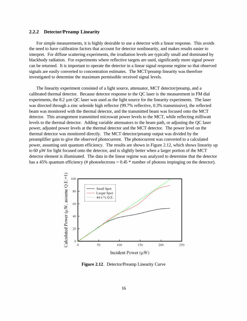
2.2.2 Detector/Preamp Linearity For simple measurements, it is highly desirable to use a detector with a linear response. This avoids the need to have calibration factors that account for detector nonlinearity, and makes results easier to interpret. For diffuse scattering experiments, the irradiation levels are typically small and dominated by blackbody radiation. For experiments where reflective targets are used, significantly more signal power can be returned. It is important to operate the detector in a linear signal response regime so that observed signals are easily converted to concentration estimates. The MCT/preamp linearity was therefore investigated to determine the maximum permissible received signal levels. The linearity experiment consisted of a light source, attenuator, MCT detector/preamp, and a calibrated thermal detector. Because detector response to the QC laser is the measurement in FM dial experiments, the 8.2 µm QC laser was used as the light source for the linearity experiments. The laser was directed through a zinc selenide high reflector (99.7% reflective, 0.3% transmissive), the reflected beam was monitored with the thermal detector, and the transmitted beam was focused onto the MCT detector. This arrangement transmitted microwatt power levels to the MCT, while reflecting milliwatt levels to the thermal detector. Adding variable attenuators to the beam path, or adjusting the QC laser power, adjusted power levels at the thermal detector and the MCT detector. The power level on the thermal detector was monitored directly. The MCT detector/preamp output was divided by the preamplifier gain to give the observed photocurrent. The photocurrent was converted to a calculated power, assuming unit quantum efficiency. The results are shown in Figure 2.12, which shows linearity up to 60 µW for light focused onto the detector, and is slightly better when a larger portion of the MCT detector element is illuminated. The data in the linear regime was analyzed to determine that the detector has a 45% quantum efficiency (# photoelectrons = 0.45 * number of photons impinging on the detector).

Figure 2.12. Detector/Preamp Linearity Curve

17

While the low return levels in diffuse scattering experiments guarantee operation in the linear regime, it can become necessary to attenuate the laser in applications with retro-reflective targets. In some cases, this can aid alignment and noise mitigation. For instance, one method of attenuating the return signal in retro-reflecting applications is to overfill the retro and detector. In addition to reducing the detected power levels to the linear regime, overfilling minimizes the sensitivity to vibrations.

3.0 FM DIAL Experiments In addition to the detailed measurements of FM DIAL component characteristics described above, a series of preliminary laboratory and outdoor FM DIAL experiments were conducted during FY02. The primary purpose of these experiments was to gain enough experience with field FM DIAL measurements to identify the most important phenomena limiting the range, sensitivity, and selectivity of our system in its envisioned operating configurations, permit a first round of system optimization, and develop some basic data collection and analysis techniques in preparation for more definitive experiments in FY03. To that end, the cart system was used successfully in three distinct configurations: monostatic, bistatic, and perimeter. These are illustrated in Figure 3.1.

Figure 3.1. Experimental Configurations Used with the FM Lidar System

18

In the monostatic configuration, the beam is directed toward diffuse scattering objects in the ambient background such as trees, buildings, hillsides or other terrain features, or vehicles. For our experiments, we often used a foam target to facilitate operating at different ranges without moving the lidar. The bistatic configuration requires a retro reflector to be deployed at some distance from the cart, but offers greatly increased return levels. Typically, a 2-in. or 6-in. retro reflector was mounted on a tripod and placed at distances ranging from 100 m to 2.5 km from the cart. The perimeter-monitoring configuration requires multiple mirrors to be carefully placed and aligned. The beam reflects off each mirror and proceeds toward the next, until it comes back to the cart. Setup time for the monostatic experiment can be as short as 10 minutes. The bistatic experiment takes about 15 minutes to set up because the retro has to be positioned. Perimeter experiments are slightly more difficult because several mirrors have to be aligned to bring the laser beam back to the cart. Alignment can be accomplished in about 20 minutes if two people are available, but can take a single experimenter up to 1 hour. These three experimental configurations provide enough diversity to cover many possible applications from covert sensing to fence line monitoring.

3.1 Monostatic Experiments The most important measurements from a chemical sensing lidar are the quantity of a probed chemical along the detection path (sensitivity), and selectivity between the target chemical and interferents. The sensitivity may be reported with many different units but the most fundamental for path-integrated absorption measurements is the concentration path length (e.g., molecules/cm2 or torr×m). Many other units are used depending on the application and required results. For instance, chemical detection in ppm×m, toxicity level, and mg/m3 are important for monitoring harmful chemicals. Infrared chemical sensors are sensitive to the absorbance integrated over the path length, and that quantity must be transformed into a concentration measurement. Because the measured quantity is absorbance, it is natural to describe the sensitivity of the instrument in terms of the noise equivalent absorbance (NEA). From that quantity, it is straightforward to determine the concentration × path length sensitivity of any chemical through the use of line strength factors. A study of the selectivity for the FM DIAL system has not been performed in FY02, but will be investigated in FY03. For the wavelengths used for nitrous oxide detection, no significant backgrounds were observed in field experiments. Therefore, the detection capability of the FM DIAL system should approach the detection sensitivity as measured, although as more interferents are allowed the detection capability may be degraded. A measurement of the NEA of the FM lidar system was performed and reported recently (Harper et al. 2002). While the details will not be given here, it is useful to point out several facts about the experiment. Foremost, this experiment was performed outside under real remote sensing conditions, as shown in Figure 3.2. The path length was 40 m (to the scattering target), and the signals that were scattered off a foam target were collected with a 10-in. telescope. Data for this nitrous oxide chemical release experiment is presented in Figure 3.3.

19

Figure 3.2. Preliminary Monostatic Field Experiment Test. The foam scattering target is 14 in.2 and located approximately 40 m from the cart.

Figure 3.3. Experimental Data Collected During Field Experiments from a 40 m Monostatic Experiment. The large derivative signal at 0.075 s is due to the nitrous oxide release, while the smaller peak at 0.055 s is due to ambient water absorption.

Over the past year, an absorption estimator was developed that may be applied directly to the lock-in output of the sensor. This algorithm was used in the determination of the NEA and is described in the report on detection sensitivity (Harper et a. 2002). After 10 seconds of data collection, the NEA, for the

20

derivative absorption feature at 0.08 s, was determined to be 4×10-4 absorbance units. It is worth pointing out that this NEA is limited by background thermal radiation, and can therefore be decreased (resulting in improved detection sensitivity) by increasing laser power, using a narrow-band filter with improved detectors and preamplifiers, optimizing laser divergence and receiver field of view, or using a retro-reflector to increase the signal return level. The use of intensity noise reduction techniques described in Section 4.1 could also decrease the NEA further. Additional details about the sensitivity experiments are given in another report (Harper et al. 2002). Because the power levels of the QC laser used in this work are ≤100 mW, the typical range for useful monostatic experiments is currently limited to <200 m. Under some circumstances, targets of opportunity (objects with favorable laser-scattering properties) may allow this range to be extended. Scattering from an air intake on a nearby building produced significant signal levels at 190 m and suggested that longer distances could be used. At these short ranges, laser speckle has been found not to play a significant role because there is a lack of range depth over the imaged area (<26 cm diameter). At much longer ranges (>1 km) significant range depth may be present; however, with 100-mW transmitted power, there is not enough returned power to obtain useful signal levels. In FY03, we plan to measure the detection sensitivity as a function of range. Long-range monostatic experiments are not currently feasible, even with more powerful lasers; however, shorter-range systems along with miniaturized systems are still viable. Development of a more powerful QC laser device (1 W) could extend the range by more than a factor of three. Lower noise detectors and preamplifiers (0.5 pA/Hz1/2) could also increase the range by a factor of two.

3.2 Bistatic The bistatic configuration has the advantage of much larger return signals as compared to monostatic experiments. While a retro-reflector must be deployed in the field, this may be possible in many operational scenarios. Because there are larger return signal levels, wider bandwidth detection may be used, which allows faster scans over absorption features. Retro-reflector experiments have been conducted at ranges between 0.2 km and 5 km (round trip). Numerous chemical sensing experiments have been performed, including nitrous oxide chemical release and monitoring of ambient water vapor. Figure 3.4 shows the returns from the retro-reflector, while monitoring ambient water vapor. The data consists of a 512-trace average collected at 200 Hz. This data is analogous, but with higher signal levels, to data from the monostatic experiments. The derivative line-shape for water is observed in Figure 3.4 near 3.5 ms, and corresponds to a peak absorbance of 0.1. While these experiments produce much higher signal levels than the monostatic experiments, retro-reflector experiments are currently limited by atmospheric turbulence rather than background thermal radiation. These turbulence effects are similar to visual distortions observed over a road on a hot day. While these effects will always be present in a remote sensing experiment, turbulence noise can be significantly reduced using the normalization scheme described in Section 4.1, and will be investigated in detail in FY03. Scanning over absorption features rapidly, using increased bandwidth, and then averaging scans together significantly reduced noise due to turbulence and vibrational effects. Because of the rapid

21

Figure 3.4. Bistatic Experiment over a Range of 1.0 km One-Way. A water signal was observed at about 3.5 ms in the scan. This trace is the result of averaging 512 individual scans, but did not employ the intensity normalization scheme.

scan time (200 Hz) and extent of averaging, the trace in Figure 3.4 does not show excessive intensity noise. At longer ranges the intensity noise problem becomes more significant, and will have to be treated appropriately. The bistatic experiments have not only shown feasibility, but have also brought up some potential limiting problems. Atmospheric turbulence appears to be a much more significant problem than the theoretical model currently predicts. While the atmospheric structure coefficients used in the modeling seemed to be appropriate for the conditions that the measurements were made, it may be necessary to measure the parameters experimentally. The experiments at 5-km round trip showed encouraging results that indicate that it should be possible to go to significantly longer ranges with the existing equipment (i.e., 10-in. telescope). Work in FY03 will focus on quantitatively measuring the detection sensitivity and range dependence for the bistatic configuration. The intensity noise reduction techniques, presented in Section 4.1, will be incorporated in a data acquisition program. This should help discriminate against atmospheric turbulence noise.

3.3 Perimeter Monitoring The perimeter-monitoring configuration can potentially be used for fence-line applications such as industrial monitoring or facility defense. This configuration was demonstrated by using two mirrors to direct the laser beam from the FM lidar cart, around a volleyball court, and back to the cart (115-m perimeter). Using the sensor in this configuration, chemical signals from ambient water vapor or released nitrous oxide were monitored. A simple gas release apparatus, which injected nitrous oxide directly into the beam-path, was employed for these preliminary experiments.

22

An averaged data trace (of 256 traces collected at 100 Hz) showing the detection of released nitrous oxide is presented in Figure 3.5. This data is analogous to the monostatic results from Harper et al. (2002). Two derivative line-shapes are observed at 0.005 s and 0.009 s. The stronger peak corresponds to an absorbance of 0.09, with a signal-to-noise greater than 150. This absorbance corresponds to 3.4 torr×m concentration path length. The NEA was not investigated in detail, but estimates from the preliminary data indicate that it is below 6×10-4, for a measurement time of 2.5 s. This level of sensitivity already provides a detection limit of 30 ppm×m for nitrous oxide.

Figure 3.5. Perimeter Monitoring Configuration Used to Detect a Nitrous Oxide Chemical Release. There are two absorption features observed in this trace located at 0.005 s and 0.009 s.

During the course of these preliminary experiments, several problems limiting system performance were observed. The first problem observed was vibration of the perimeter mirrors, which becomes increasingly important at larger perimeters. For these tests, flat mirrors were used to reflect the beam around the perimeter. Small vibrations in the mirror cause the reflected beam to vary in direction, causing a portion of the beam to miss the next mirror. This causes the received laser beam intensity to vary with time, because of mirror losses. A potential way to correct this problem, and help eliminate noise due to vibrations, is to use convex mirrors with long focal lengths. After a collimated beam reflects off the convex mirror surface, it becomes slightly divergent. The diverging beam then overfills the next mirror, and small vibrations in the first mirror will not cause the beam to miss the second mirror. The radius of curvature of the first mirror can be optimized so that a minimum amount of the beam is lost due to overfilling, while ensuring that vibrations will not cause the beam will miss the second mirror. When high concentrations of nitrous oxide were released, additional turbulence was generated and interfered with visible and infrared radiation. This noise was caused by the interface index mismatch and

23

density mismatch between nitrous oxide and air as the gas was released into the atmosphere. Because pure nitrous oxide was slowly released into the beam path, this effect was maximized. A more appropriate method of releasing gas samples has been developed and should provide a more realistic gas release for work in FY03. The improved apparatus includes a fan for premixing chemicals with air before introduction into the beam path. This should help correct for the gas interface intensity noise problems that were observed. The third problem is due to atmospheric turbulence, which was found to be larger than that predicted by the theoretical modeling. The turbulence caused fluctuations in the returned laser beam, which degraded the quality of the data. For larger perimeters, this problem becomes more substantial. While this problem cannot be corrected, we have developed methods that reduce the sensitivity to these deleterious noise effects. This data treatment is described in Section 4.1. In FY02 we demonstrated that the FM-DIAL system could be operated in a perimeter-monitoring configuration. The demonstration included a 115-m perimeter that encompassed a volleyball field and detected nitrous oxide chemical releases from within the perimeter. Additional experiments aimed at quantitatively measuring the detection sensitivity still need to be performed. The range of perimeters that can be monitored needs to be evaluated, along with how detection sensitivity changes with perimeter distance. Solutions for reducing vibrations of the perimeter mirrors need to be implemented and tested. Further improvements are likely to be realized using techniques to reduce the intensity noise and optimizing the perimeter optics.

4.0 Detection/Data Processing Development In addition to transmitter and detector modules, it is necessary to have data processing algorithms that handle the returned signals and convert them into concentration estimates. The lidar system operates using a frequency-modulation technique that incorporates narrow bandwidth lock-in detection, allowing signals to be monitored continuously. For FY02, the data processing falls into two categories—noise reduction and concentration estimation. Monostatic experiments involving diffuse scattering are already operating at shot-noise-limited (from blackbody radiation, i.e., BLIP) levels, whereas the bistatic and perimeter experiments are limited by atmospheric turbulence noise. An active normalization treatment has been developed to help reduce the effects of atmospheric turbulence. Initial tests show that this technique works well in eliminating intensity noise in the returned beam. Each of the three configurations has also benefited from the development of a concentration estimation method. This method utilizes RAM, normally thought of as a nuisance in frequency modulation measurement techniques, to gauge the magnitude of returned signal. This, along with the results from lock-in detection, allows calculation of absorbance and concentration estimation. This work, along with a sensitivity analysis, has already been described in a recent report (Harper et al. 2002). We have pursued an experimental verification of the concentration estimation treatment and noise reduction techniques.

24

4.1 Intensity Noise Mitigation Significant advances have been made in the detection and data processing experiments. One of the key problems in remote sensing is that it is inherently a single beam experiment, where it is difficult to remove or account for the effects of fluctuations in the intensity of the return beam. This problem is exacerbated by atmospheric turbulence, which causes significant fluctuations in the return beam at distances greater than 100 m. This turbulence is the same as that seen when looking into the distance over a hot highway. In bistatic and perimeter configurations, which have large signal returns, turbulence noise dominates other sources of noise. Recently, we have developed a detection scheme that will help discriminate against intensity noise. Initial experiments showed promising results; however, a more thorough investigation still needs to be performed. These turbulence effects are present in DIAL and FM DIAL systems, resulting from atmospheric fluctuations that interfere with the beam. In DIAL experiments, one of the simplest ways to counter this problem is to have two laser wavelengths—one on resonance and one off resonance—that are separated by sub millisecond timescales (Menyuk and Killinger 1981). During these short timescales, atmospheric turbulence (which changes on slower timescales) is effectively frozen. The problem is similar for FM DIAL, and data should be collected on timescales shorter than atmospheric turbulence effects. FM experiments using QC lasers also have additional advantages that can be used to eliminate intensity noise effects. From the frequency modulation measurements presented in Section 2.1.3, it was found that the FM component of the modulation lags the AM component by 45° at 200 kHz. By adjusting the phase of the lock-in detector so that it is optimized for the FM phase, both the full FM and part of the AM are detected. The orthogonal signal collected simultaneously consists only of the AM signal. Because both of these signals are proportional to the returned power, dividing the FM optimized signal by the orthogonal signal accomplishes normalization of the returned power. Laboratory demonstrations of this new technique have successfully shown this to be a useful approach for reducing the effects of turbulence-induced noise. The results of a simple laboratory experiment illustrate the power of this technique. The QC laser output was directed toward a foam scattering target 2.5 m from the QC laser. Scattered light was collected with the telescope receiver and imaged onto a MCT detector. A gas cell (15 cm) containing 100 Torr of nitrous oxide was placed in the beam path to provide absorption features. The laser was tuned across two absorption features by ramping the drive current. A chopper wheel was placed partially in the beam path and attenuated the beam intermittently. This attenuation is observed in the black trace of Figure 4.1 as sharp dips in the signal level. Dividing by the orthogonal trace (not shown) for power normalization yielded the trace shown in red. The red trace does not contain any of the intensity dips as seen in the original data. A close examination of the red trace reveals slightly larger noise during the time that the beam is attenuated. This results from how signal-to-noise levels propagate through the calculation and is entirely expected. Each trace, FM optimized and orthogonal, has a signal to noise determined by the signal level and the noise floor. As indicated in Section 2.2.1, the noise is dominated

25

Figure 4.1. Noise Reduction Demonstration. The black data shows the results from lock-in detection of

signal and noise. The red trace shows the intensity-normalized ratio, eliminating the intensity noise.

by background radiation, which is constant over the entire data trace. Further, the noise is the same for both traces. The signal to noise for each point in the traces is determined by the signal level for that point. For the simple ratio of two numbers (each with a given uncertainty)

bbaa

f∆±∆±

= ,

the following expression holds for the statistical uncertainty of f :

( ) ( )22

22

21b

ba

ab

f ∆

+∆

=∆ .

For the case where the uncertainties are the same (∆a=∆b),

22

1

∆

+

∆

=∆

bb

aaf

f.

This equation shows that the signal to noise of f is degraded to the lesser of the signal to noise of a or b. For intensity fluctuations that reduce the amount of each signal, the signal to noise for the ratio is decreased by the same factor. This explains why the noise levels in Figure 4.1 are

26

slightly larger when the beam is attenuated. In FY03, plans are being made to implement a computer interface that will collect and average this ratio data appropriately, using weighted averaging and propagation of errors. This type of averaging will give higher weights to data with larger return signals and smaller weights to weaker return signals. This procedure will cause noise to be averaged away more rapidly than with simple averaging. Similar experiments were also performed using second harmonic detection, normalized by the first harmonic signal. This collection scheme requires locking the laser to an absorption feature, recording the 1f and 2f signals, and calculating the ratio. This approach helps, but does not eliminate all of the intensity fluctuations in a remote sensing experiment because the 1f and 2f signals respond differently to the fluctuations. It also has the disadvantage that the laser cannot be scanned over an absorption feature.

4.2 Quantitative Signal Verification To have confidence in measurements from the FM lidar system, it is necessary to test and verify the data acquisition algorithms and processes. The best way to do this is to monitor a known concentration of a gas sample, apply the appropriate algorithms, and compare sensor measurements with the known concentration. To verify the methods used, experimental conditions were selected so that direct absorption signals could be observed simultaneously with lock-in detection of nitrous oxide absorptions. These conditions required significant absorption signals (0.1 absorbance) and small modulation index (0.0003 cm-1). The output from the QC laser was split into two beams using zinc selenide beam splitters. The first beam was directed through a 15.5-cm gas cell filled with nitrous oxide (1.02 Torr) and centered on an MCT detector. A second beam was directed through a reference etalon (FSR = 0.025 cm-1) and centered on a second MCT detector. The laser was modulated at 201 kHz and scanned over the full tuning range (~1.5 cm-1). The collected data consisted of the time-dependent signals from the MCT and the QC laser drive current. The first test was to compare the observed direct absorption signals with the calculated line-shape and intensity. Figure 4.2 shows the agreement between the calculated and observed direct absorption feature. The calculated trace was generated using only the gas cell length and the nitrous oxide pressure in the gas cell, which determines the intensity and the width of the feature. The agreement between measured and calculated line-shapes and intensities is excellent. This shows agreement between the added gas concentration and the observed signals. Experimental line-shapes were measured and compared to predicted line-shapes at low pressure (1 Torr), high pressure (100 Torr), and atmospheric broadened features (100 Torr buffered with air up to 1 Atm). Similar measurements were made to compare lock-in detection signals with data derived from the direct absorption scans. Derivatives of the direct data traces with respect to optical frequency were taken for the comparison (dVdirect/dν). The lock-in traces (dV lock-in/di * ∆i) were divided by the current modulation and the frequency derivative (dν/di) to obtain (dVlock-in/dν). These transformations allow comparison between the direct and lock-in traces as shown in Figure 4.3. Agreement is excellent between the observed and predicted signals, as shown in Figure 4.3, reiterating the quantitative understanding of the sensor output.

27

Figure 4.2. Agreement Between the Absorption Calculated from the Added N2O Pressure and the Observed Direct Absorption Signal

Figure 4.3. Agreement Between the Observed Lock-in Detection Results and the Signal Calculated from the Direct Absorption Experiment

One of the main advances made this year is the capability to transform the detected signal-to-concentration path length measurements. Absorbance measurements require measuring the number of incident photons (or alternatively, transmitted photons) and the number of photons absorbed. In FM experiments, the derivative signal is proportional to the number of photons absorbed; however, the number of photons transmitting through the sample is more difficult to determine. RAM, which is

28

typically thought of as a nuisance or problem in detection strategies, has provided a useful way to determine the number of transmitted photons. Modulating the QC laser produces a characteristic amount of RAM, which can in turn be measured by the receiver/detector. The amount of RAM observed by the detector is proportional to the total number of laser photons received. Because the proportionality constant can be measured, lock-in detection provides a measurement of the transmitted photons, as well as the number of absorbed photons. This allows calculation of absorbance, and ultimately, concentration measurements. Additional details pertaining to the concentration estimator method have been presented in another report (Harper et al. 2002).

5.0 Future Plans The main experimental goal for FY03 is to improve the FM lidar system to the point that quantitative comparison of theory and modeling can be performed to validate PNNL’s numerical model. Validation experiments will be performed in a field environment from the new lidar trailer. Additional tests and validation of the theoretical modeling will be performed through comparison to detailed field experiments in the monostatic, bistatic, and perimeter monitoring configurations. Performance of the system will be measured for each of the configurations and related to detection sensitivities for relevant chemical species. The trailer platform is also capable of supporting the FTIR sensor system and will provide the opportunity to use both sensors in tandem. The noise reduction techniques presented in this report will be investigated more thoroughly, in particular for applications with reflective targets. A computer-controlled data acquisition program will be developed to operate the data collection, provide the capability of accumulating the data collected for each of the experimental configurations, and provide real-time concentration estimates. Chemical release experiments will be used to investigate the capabilities and performance of the FM lidar system. One of the main drawbacks of the QC lasers is the lack of spectral tunability. Injection current tuning may be used to rapidly tune or modulate a QC laser, but gives at most about 1.5 cm-1 of tunability. Temperature tuning has not been explored yet, but offers the capability to tune the QC laser, although only at slow speeds. In FY03, a multiple wavelength lidar system will be explored by combining the output from two or three lasers to form the transmit beam. The received signals will be detected using a single detector using lock-in detection at unique modulation frequencies. Multiple wavelength detection should help both the detection sensitivity and background discrimination. Multiple wavelength detection may also give the opportunity to detect spectral features that are wider than the tuning range of a given QC laser. While a long-range monostatic FM lidar system is not feasible with the current QC laser technology, it may become so in the future. QC lasers have made rapid advances toward operating at higher powers as well as approaching room temperature operation. A potential area of interest is to try to leverage one of the biggest advantages of QC lasers—their small size. In the lidar system, most of the size is due to having an optical table, telescope, and detection electronics. For short-range and retro-reflector applications, a large telescope is not necessary to collect sufficient returned signals. Furthermore, the detection electronics could be much smaller than the commercial components that are convenient to use for the laboratory and trailer experiments.

29

6.0 References Cannon BD, WW Harper, TL Myers, MS Taubman, RM Williams, and JF Schultz. 2001. Progress Report on Frequency - Modulated Differential Absorption Lidar. PNNL-13736, Pacific Northwest National Laboratory, Richland, WA. Harper WW, DM Sheen, and JF Schultz. 2002. FM-DIAL Preliminary Detection Sensitivity Measurements. PNNL-13992, Pacific Northwest National Laboratory, Richland, WA. Martini R, R Paiella, C Cmachl, F Capasso, EA Whittaker, HC Liu, HY Hwang, DL Sivco, JN Baillargeon, and AY Cho. 2001. Electron. Lett. 37, 1290. Menyuk R and DK Killinger. 1981. Optics Lett. 6, 301. Schultz JF. 2002. Final Report - Airport Chemical Threat Project PNNL Project Number 40826. PNNL-14007, Pacific Northwest National Laboratory, Richland, WA. Sheen DM. 2000. FM Spectroscopy Modeling for Remote Chemical Detection. PNNL-13324, Pacific Northwest National Laboratory, Richland, WA.