Remote Magnetometry with Mesospheric Sodium by the laser light after any collision, because its...

Remote Magnetometry with Mesospheric Sodium

ONR Remote Atmospheric Magnetometry Workshop25 April 2014FASORtronics LLCContract N00014-14-C-0110

Tom Kane Craig Denman Paul Hillman

1

Friday, April 25, 2014

Goals of Talk

• Understand measurement sensitivity

• Scaling rules for sensitivity

• Technology of experiment

• Update on experimental program

• Magnetometry and guidestar laser technology

2


Laser Remote Magnetometry using Natural Sodium

3

• The Sensor• sodium atoms in the

mesosphere• 3000-5000 atoms/cm3 • 90 kilometer altitude

• Laser Interrogation of atoms• pulse laser near Larmor

frequency (~350kHz) • detect returned photon

fluorescence

• Laser similar to astronomical “guidestar” lasers

J.M. Higbie, et al, arXiv:0912.4310v1 [physics.atom-ph] 22 Dec 2009


The 350 kHz Larmor frequency corresponds to a 0.5 Gauss (50 µTesla) magnetic field, which is near the high extreme over the earth. This frequency is proportional to the B field.

Photon Limited Sensitivity

4

• N = expected number of photons collected during measurement

• √N = standard deviation in number of photons, “shot noise”

• 1/√N = fractional uncertainty

FWHM~150 nanotesla

Sign

al, P

hoto

nsPeakSignal

Frequency, ~350 kHz, or Field, ~50 µtesla

MaximumdN/dB

Magnetic field change equivalent to shot noise:

Roughly: ∆B = (1/√N) / (dN/dB / N)(1/1000) / (1%/nanotesla) = 0.1 nanotesla


The resonance is expected to be about 1 kHz wide, corresponding to about 150 nTesla. The point of steepest slope will have a slope of about 1% of signal per nTesla. With 1 million photons detected, and only shot noise, there is measurement uncertainty of 0.1%. Thus with 1 million photons detected, the magnetic field change equivalent to shot noise is about 0.1 nTesla. This case is for an optimized laser.

Sensitivity of Mesospheric Sodium Magnetometry

5

4 3FWHM9

Peak + Back|Peak ! Back |

nT / !Hz =

FWHM

Sign

al, P

hoto

n/se

cond

PeakSignal

Field, ~50 µtesla

BackgroundSignal


The equation is the shot-noise-limited sensitivity, assuming a Lorentzian lineshape. FWHM is the full-width at half-maximum of the resonance, in units of nTesla. Peak and Back are the signals at the peak of the resonance, and away from the resonance, in units of photons per second.

What Determines Linewidth?

• Rate of Loss of polarized atoms• 1 / Linewidth ≈ Decay time of polarized atoms

• Collisions with molecules

• Atoms moving out of laser beam

• Laser beam moving

• Rate of build-up of polarized atoms• Too much laser intensity broadens linewidth

• There is an optimum

6


The two types of collisions

• All collisions change velocity• Atom is “lost” only if laser is single-frequency

• 50 microseconds mean time between collisions @ 100 km

• Only some collisions change spins (polarization)• Collisions with oxygen (O2)

• Atom is lost

• 250 microseconds mean time between collisions with O2

• Collision rate is linear in pressure• Mesospheric pressure 10-6 of sea level

7


The linewidth of the resonance is determined by how long an atom sees the laser light before its spin is randomized. For a narrow-band laser, the atom stops being pumped by the laser light after any collision, because its velocity is changed to where its Doppler shift puts the laser light outside the sodium absorption. But with a broadband laser, the Doppler shift does not stop the pumping process,because light is present over the whole Doppler-broadened laser line. For a broadband laser, only collisions with oxygen will stop pumping, since the oxygen will exchange angular momentum with the sodium atom. Thus a broadband laser can narrow the linewidth by a factor of 5, improving magnetic sensitivity.

If Laser Linewidth ≥ Atom Doppler Linewidth

• Longer Lifetime applies

• ~1 GHz easily created by phase modulation

• Fiber-coupled, waveguide phase modulators

8

Phase Mod

frequency

Tfrequency

1/T

+90°

-90°

Nonlinear

Conversion

Amplifier"Random" Phase modulation

through 180° can broaden linewidthLinewidth ≈ Data Rate


Phase modulation of the laser can broaden linewidth in a very controllable way. However, high-frequency phase modulators are not available in bulk form. They are available in waveguide form, which is not compatible with power above a few milliwatts, or with visible light. An architecture which phase-modulates at low power, in the infrared, and then amplifies and frequency-converts afterward, can provide broad linewidth, at high power, at 589 nm.

Optimum Intensity

• Intensity too low:• Time to polarize atom >> spin exchange time

• Few atoms polarized

• Intensity too high:• Time to polarize atom << spin exchange time

• Polarization saturates; linewidth broadens

• Low value of optimum intensity leads to cheap, simple launch telescope• Commercial asphere lens is adequate

9


Launch telescope can be about 100 mm diameter.

Effect of Laser Spectrum

10

Laser SpectrumOptimum Average Intensity*

nanoteslas/!Hz @

2 watts avg.

nanoteslas/!Hz @

20 watt avg.

Single Frequency0.2 watt/

m2 6 2

Single Frequency + Repump

0.6 watt/m2 2.5 0.8

Broad Linewidth + Repump

8.5 watt/m2 0.34 0.11

*Average Intensity = time averaged over modulation cycleModeling: Rochester Scientific pulsed code


Our initial work will be with a 2 watt laser, narrow linewidth, with no "repump" sideband. Expected sensitivity is near 6 nTesla/√Hz. A 20 watt laser, with optimum spectral properties, could go down to 100 picoTesla /√Hz.

Factors Extrinsic to Atoms

• Goal: Return of order 106 photons per second• Atomic density

• Scatter fraction

• Collection geometry

• Range & telescope aperture

• Laser power

• Detector efficiency

11


Collection Geometry

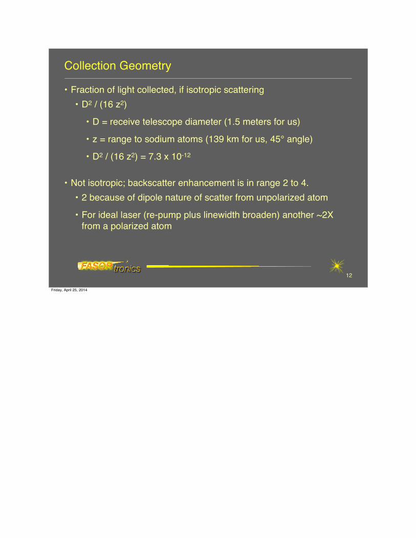
• Fraction of light collected, if isotropic scattering• D2 / (16 z2)

• D = receive telescope diameter (1.5 meters for us)

• z = range to sodium atoms (139 km for us, 45° angle)

• D2 / (16 z2) = 7.3 x 10-12

• Not isotropic; backscatter enhancement is in range 2 to 4.• 2 because of dipole nature of scatter from unpolarized atom

• For ideal laser (re-pump plus linewidth broaden) another ~2X from a polarized atom

12


Sodium Layer

• “Column Density” - per area• 40 million atoms/mm2

• Volume: 4 atoms/mm3

• Fraction of light scattered: 4%

• Total worldwide sodium: 800 kilograms

• Lifetime in mesosphere• Weeks

13


Laser Power & Detection Efficiency

• 50 watts is state-of-art for 589 nm

• Our project:• 10 watts x 20% duty cycle = 2 watts

14


In a later phase we hope to upgrade to 20 watts of transmitted power.

4 Nov 20122012 CfAO Fall Science Retreat - Laser Workshop

Laser Design to Obtain Beam Pulse Format

15

Ytterbium-dopedfiber amplifier

Fiber-coupledmodulators

1 µmoscillator

LBO589 nm output

1.3 µm resonator

=589 nm light=1.3 µm light=1 µm light

1.3 µmoscillator


This fiber / YAG "hybrid" design will provide an efficient laser pulsed at the right frequency for magnetic measurements. Since the 1 µm light is converted in a single pass, and is not resonant, its modulation will be passed directly to the generated 589 nm light, rather than stripped off by the filtering properties of the resonator. Thus any modulation at 1 µm appears directly at 589 nm. So a broad linewidth, or sidebands, can be generated using low-power, infrared phase modulators, and transferred to the high-power 589 nm.

Photodetectors that are shot-noise limited

16

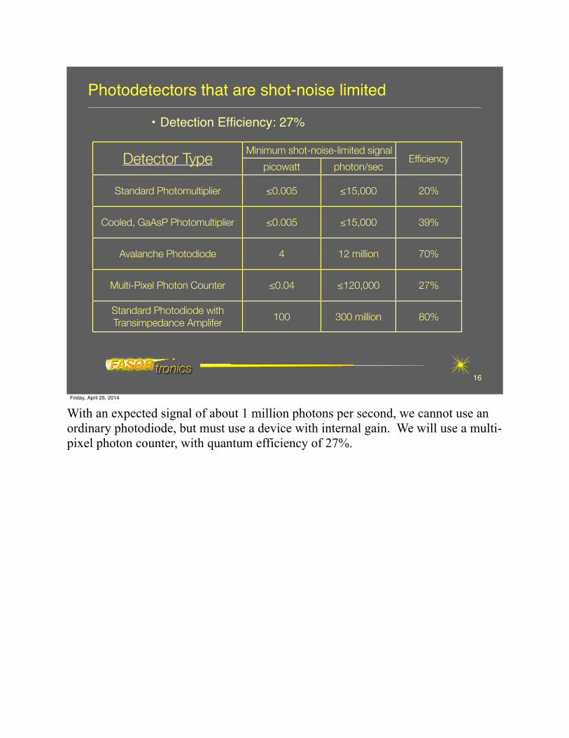
Detector TypeMinimum shot-noise-limited signalMinimum shot-noise-limited signal

EfficiencyDetector Typepicowatt photon/sec

Efficiency

Standard Photomultiplier !0.005 !15,000 20%

Cooled, GaAsP Photomultiplier !0.005 !15,000 39%

Avalanche Photodiode 4 12 million 70%

Multi-Pixel Photon Counter !0.04 !120,000 27%

Standard Photodiode with Transimpedance Amplifer

100 300 million 80%

• Detection Efficiency: 27%


With an expected signal of about 1 million photons per second, we cannot use an ordinary photodiode, but must use a device with internal gain. We will use a multi-pixel photon counter, with quantum efficiency of 27%.

Our Team: FASORtronics + University of Arizona

17

Steward Observatoryʼs 61” Kuiper Telescope

Laser owned by Air Force


University of Arizona partners: Michael Hart and Randy "Phil" Scott

The Telescope: University of Arizona 61-inch “Kuiper”

18

~ 1.55 meter


Reference Magnetometer: USGS “Observatory”

19

~0.1 nanoTesla noise, 1 sample per second


The USGS data, Tucson observatory, is posted on the net. http://magweb.cr.usgs.gov/data/magnetometer/TUC/OneSecond/

http://magweb.cr.usgs.gov/data/magnetometer/TUC/OneSecond/

http://magweb.cr.usgs.gov/data/magnetometer/TUC/OneSecond/

Expected Signal on Magnetic Storm Day

20

Data from USGS,Jan 22, 2012

Added noise of 4 nT √Hzdoes not cover signal


Even with our non-optimized laser, we should easily be able to see a magnetic storm. Shifts of many nanoTesla, over hours, should be readily observed, if the laser is reliable.

Expected Signal on Typical Quiet Day

21

47802.8

47803

47803.2

47803.4

47803.6

47803.8

47804

47804.2

0 100 200 300 400 500 600 700 800 900 1000

Seconds

nanoTesla

With NoiseNo Noise

Data from USGS,

April 14, 2012

Added noise of 0.2 nT √Hzdoes not cover signalfor >30 sec


An optimized laser should be able to see the change which typically occurs in 30 seconds, on a magnetically quiet day.

Date post:	01-May-2018
Category:	Documents
Upload:	phungxuyen
View:	216 times
Download:	2 times

Remote Magnetometry with Mesospheric Sodium by the laser light after any collision, because its...

Documents