Contents lists available at SciVerse ScienceDirect
Remote Sensing of Environment
j ourna l homepage: www.e lsev ie r .com/ locate / rse
An algorithm to retrieve absorption coefficient of chromophoric dissolved organicmatter from ocean color
Qiang Dong a, Shaoling Shang a,b,⁎, Zhongping Lee c
a Research and Development Center for Ocean Observation Technologies, Xiamen University, Xiamen 361005, Chinab State Key Laboratory of Marine Environmental Science, Xiamen University, Xiamen 361005, Fujian, Chinac Environmental, Earth, and Ocean Sciences, University of Massachusetts at Boston, MA 02125, USA
⁎ Corresponding author at: Research and DevelopmenTechnologies, Xiamen University, Xiamen 361005, Chin
We extended the quasi-analytical algorithm (QAA) architecture to analytically derive absorption coefficientof chromophoric dissolved organic matter (ag). Specifically, we used an empirical formula based on total ab-sorption and particle backscattering coefficients to estimate and then remove detritus absorption coefficient(ad), and developed a scheme to use absorption coefficients at three wavelengths (412, 443, and 490 nm) forthe separation of ag and aph (absorption coefficient of phytoplankton). The algorithm was tested using an insitu data set collected in the South China Sea and the Taiwan Strait and a global in situ data set—the NASABio-Optical Marine Algorithm Data set (NOMAD). Our results indicated that this new analytical algorithmfor retrieving ag performed reasonably well with a mean absolute percentage error of approximately 45%for ag(412), while it also presented a satisfactory performance for aph and ad in both coastal and oceanic wa-ters. Furthermore, the applicability of this new algorithm for general oceanographic studies was briefly illus-trated by applying it to MODIS measurements over the Taiwan Strait and the shelf region near the MississippiRiver delta. Nevertheless, more independent tests with in situ and satellite data are needed to further validateand improve this innovative approach.
Gelbstoff, or chromophoric dissolved organic matter (CDOM; fre-quently used abbreviations are summarized in Table 1), is an opticallyactive component and plays an important role in carbon cycling(Coble, 2007). CDOM provides an effective sun shade, modulates theunderwater light field and thus affects the growth of phytoplanktonand other aquatic organisms (e.g., Jerlov, 1968; Karentz & Lutze,1990). In addition, CDOM makes up part of the pool of dissolved or-ganic carbon (e.g., Nelson et al., 1998; Vodacek et al., 1997). It is im-portant therefore to study CDOM, including its abundance, source,composition, and final fate at local and global scales, in order to even-tually model and forecast CDOM's variations as well as its contribu-tions to global carbon budgets (e.g., Mannino et al., 2008).
Because field studies, although quite precise and extremely useful,provide limited information in space and time, CDOM propertyobtained through satellite remote sensing is the only feasible meansto inform its distribution at global scales. In the past decades,semi-analytical algorithms to retrieve the absorption coefficients ofthe sum (adg; m−1) of CDOM (ag; m−1) and detritus (ad; m−1), col-lectively named as CDM, have been developed (Carder et al., 1999;
t Center for Ocean Observationa. Tel./fax: +86 592 2184781..edu.cn (S. Shang).
rights reserved.
IOCCG, 2006), enabling the characterization of CDM on a globalscale (e.g., Siegel et al., 2002). These algorithms, however, do not di-vide adg into ag and ad analytically, thus could not provide a preciseevaluation for the spatial and temporal variations of ag, a proxy forCDOM. Recently, Mannino et al. (2008) developed an empirical algo-rithm to retrieve ag for coastal waters in the middle Atlantic Bight, butit is not clear if the empirical coefficients are applicable to other re-gions or oceanic waters. Separately, Zhu et al. (2011) used data mea-sured in the Mississippi River plume to develop a semi-analyticalalgorithm for the separation of ag from adg and achieved some suc-cesses for their data set. The derivation of ad there followed theapproach of Lee (1994), i.e., using derived particle backscattering co-efficient (bbp; m−1) as an input to estimate ad. Our latest in situ mea-surements suggest that this approach may be reasonable for turbidcoastal waters where suspended particles are dominated by mineralparticles (e.g., Mississippi River plume), but may have limitations forwaters where particles are dominated by phytoplankton (e.g., oceanicwaters). Therefore, for the evaluation of CDOM in both coastal and oce-anic waters, there is still a lack of robust algorithm to estimate ag fromocean color satellite measurements.
Here, we propose a new approach to derive CDOM absorptioncoefficient from ocean color based on the quasi-analytical algorithm(QAA; Lee et al., 2002). The performance of the approach is assessedusing an in situ data set collected in the South China Sea and theTaiwan Strait (hereafter abbreviated as SCSD) and a global scale in
adg Absorption coefficient of detritus and CDOM m−1
ag Absorption coefficient of CDOM m−1
ap Particulate absorption coefficient (ap=aph+ad) m−1
aph Absorption coefficient of phytoplankton m−1
aphg Absorption coefficient of phytoplankton and CDOM m−1
anw Total absorption coefficient without pure watercontribution (anw=aph+ad+ag)
m−1
bbp Backscattering coefficient of suspended particles m−1
CDOM Chromophoric dissolved organic matterNOMAD NASA Bio-Optical Marine Algorithm Data setQAA Quasi-analytical algorithm (Lee et al., 2002)Rrs Above-surface remote-sensing reflectance sr−1
Sag Spectral slope for CDOM absorption coefficient nm−1
Sad Spectral slope for detritus absorption coefficient nm−1
SCSD In situ data set collected in the South China Sea andthe Taiwan Strait
260 Q. Dong et al. / Remote Sensing of Environment 128 (2013) 259–267
situ data set—the NASA Bio-Optical Marine Algorithm Data set(NOMAD; Werdell & Bailey, 2005). As comparison, the performanceof an earlier empirical-style algorithm (Mannino et al., 2008) and asemi-analytical algorithm (Zhu et al., 2011) was also assessed usingthe same data sets. The proposed algorithm is further applied to Mod-erate Resolution Imaging Spectroradiometer (MODIS) measurementsover the Taiwan Strait and the shelf region near the Mississippi Riverdelta to briefly illustrate its applicability for general oceanographicstudies.
2. Data and methods
2.1. SCSD data set
The SCSD data were collected during 10 cruises over the years of2003–2007. They included five parameters, which were remote-sensing reflectance (Rrs; sr−1), total absorption coefficient withoutwater (anw; m−1), ag, ad, and absorption coefficient of phytoplankton(aph; m−1).
The above-surface Rrs was derived from the measurements of(1) upwelling radiance (Lu; W m−2 nm−1 sr−1), (2) downwellingsky radiance (Lsky; W m−2 nm−1 sr−1), and (3) radiance from a stan-dard Spectralon reflectance plaque (Lplaque; W m−2 nm−1 sr−1). Theinstrument used was the GER1500 spectroradiometer (Spectra VistaCorporation, USA), which covers a spectral range of 350–1050 nmwith a spectral resolution of 3 nm. From these three components, Rrscan be calculated as:
Rrs ¼ ρ� Lu−F � Lskyπ � Lplaque
−Δ ð1Þ
where ρ is the reflectance of the Spectralon plaque with Lambertiancharacteristics, and F is the surface Fresnel reflectance (around 0.023for the viewing geometry). Δ(sr−1) accounts for the residual surfacecontribution (glint, etc.), which was determined either by assumingRrs(750)=0 (clear oceanic waters) or through iterative derivationaccording to optical models for coastal turbid waters, as described inLee et al. (2010).
Measurements of ag were performed according to the OceanOptics Protocols Version 2.0 (Mitchell et al., 2000), and were detailedin Hong et al. (2005) and Du et al. (2010). Briefly, seawater wasfiltered with a thoroughly cleaned 0.2-μm Millipore filter, and theabsorbance of the filtered water was measured in a 10-cm quartzcell between 250 and 800 nm with 1 nm increment using a VarianCary100 dual-beam spectrophotometer. The reference was 0.2-μm
filteredMilliQ water. After converting the absorbance to absorption co-efficient, a nonlinear least square regression (Eq. 2 with λ0=443 nm)was employed to obtain the spectral slope (Sag; nm−1) over a wave-length range from 300 to 500 nm (Bricaud et al., 1981).
ag λð Þ ¼ ag λ0ð Þ � exp −Sag λ−λ0ð Þ� �
ð2Þ
The particulate absorption coefficient (ap; m−1) was measured bythe filter-pad technique (Kiefer & Soohoo, 1982) with a dual-beam PELambda 950 spectrophotometer equipped with an integrating sphere(150 mm in diameter), in accordance with a modified Transmittance-Reflectance (T-R) method (Dong et al., 2008; Tassan & Ferrari, 1995).This approach was selected instead of the T method recommended inthe NASA protocol (Mitchell et al., 2000), because some of thesamples were rich in highly scattering non-pigmented particles; as aresult, the standard T method overestimated the sample absorption(Dong et al., 2009; Tassan & Ferrari, 1995). Coefficient ad was obtainedby repeating the measurement on samples after pigment extraction bymethanol (Kishino et al., 1985), and then aph was calculated bysubtracting ad from ap. Eq. (3) with λ0=443 was fitted by a nonlinearleast square regression to obtain the spectral slope (Sad; nm−1) over awavelength range from 400 to 600 nm.
ad λð Þ ¼ ad λ0ð Þ � exp −Sad λ−λ0ð Þð Þ ð3Þ
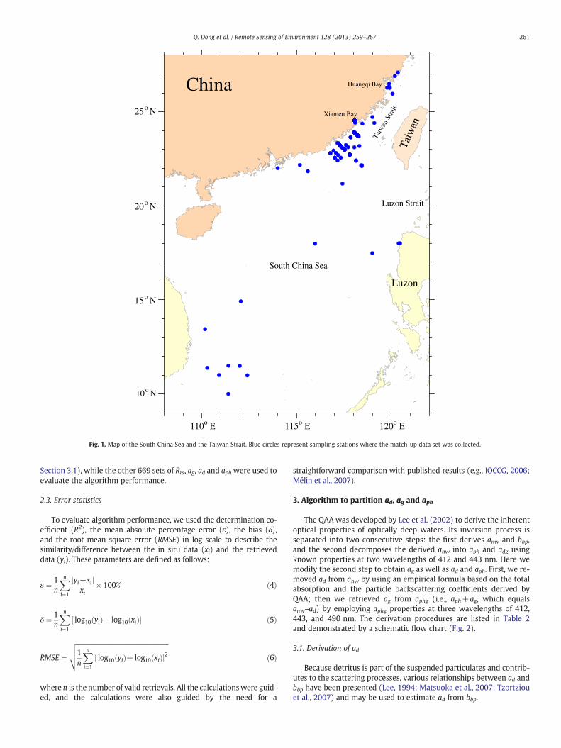
In total, there were 104 sets of in situ data, of which 86% was fromthe Taiwan Strait and the other 14% was from the South China Sea(see their locations in Fig. 1). The Taiwan Strait, a shallow channelconnecting the South China Sea with the East China Sea, has complexhydrographic conditions determined by influences of several currentsunder the forcing of monsoonal winds (e.g., Jan et al., 2002). Severalmedium-sized rivers and numerous bays are located on the westcoast (on mainland China) of the strait. Algae blooms often occur dur-ing spring in these bays (e.g., Wang et al., 2009). Also along this coast,upwelling develops in summer, driven by the prevailing southwestmonsoon, which runs parallel to the coast due to Ekman transport(e.g., Hong et al., 2009). The Taiwan Strait portion of the SCSD mainlyconsisted of summer upwelling samples, intensive algae bloom sam-ples in two bays (Xiamen Bay and Huangqi Bay), and samples in thevicinity of river mouths.
The South China Sea is one of the largest marginal seas in theworld. Its basin is deep (~5000 m) and oligotrophic, with surfacechlorophyll concentration lower than 0.1 mg/m3 except in winter(e.g., Liu et al., 2002; Shang et al., 2012). Two large rivers, the PearlRiver and the Meikong River, discharge into the South China Sea.Plume-induced blooms are often observed (e.g., Dai et al., 2008).Meso-scale eddies and upwelling events are also prominent, resultingin significant biological enhancements (e.g., Chen et al., 2007; Ganet al., 2009).
In summary, this in situ data set used for algorithm assessment cov-ered a variety of coastal and oceanic water regimes, and thus a widerange of absorption properties, with anw(443) ranging from 0.021 to2.16 m−1, and the ratios of aph(443)/anw(443), ag(443)/anw(443), andad(443)/anw(443) varying in a range of 8.9%–78.9%, 5.4%–54.8%, and6.9%–85.7%, respectively.
2.2. NOMAD data set
The NOMAD data set was downloaded from the website: http://seabass.gsfc.nasa.gov/. This is a publicly available, global, in situ bio-optical data set for use in ocean color algorithm development andsatellite data product validation activities (Werdell & Bailey, 2005).In this data set, 89 sets contain concurrent Rrs, anw, bbp and ad,which were used to derive empirical functions (see Eqs. 7–8 in
Fig. 1. Map of the South China Sea and the Taiwan Strait. Blue circles represent sampling stations where the match-up data set was collected.
261Q. Dong et al. / Remote Sensing of Environment 128 (2013) 259–267
Section 3.1), while the other 669 sets of Rrs, ag, ad and aph were used toevaluate the algorithm performance.
2.3. Error statistics
To evaluate algorithm performance, we used the determination co-efficient (R2), the mean absolute percentage error (ε), the bias (δ),and the root mean square error (RMSE) in log scale to describe thesimilarity/difference between the in situ data (xi) and the retrieveddata (yi). These parameters are defined as follows:
where n is the number of valid retrievals. All the calculationswere guid-ed, and the calculations were also guided by the need for a
straightforward comparison with published results (e.g., IOCCG, 2006;Mélin et al., 2007).
3. Algorithm to partition ad, ag and aph
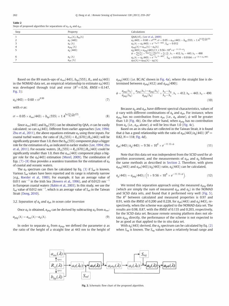
The QAA was developed by Lee et al. (2002) to derive the inherentoptical properties of optically deep waters. Its inversion process isseparated into two consecutive steps: the first derives anw and bbp,and the second decomposes the derived anw into aph and adg usingknown properties at two wavelengths of 412 and 443 nm. Here wemodify the second step to obtain ag as well as ad and aph. First, we re-moved ad from anw by using an empirical formula based on the totalabsorption and the particle backscattering coefficients derived byQAA; then we retrieved ag from aphg (i.e., aph+ag, which equalsanw–ad) by employing aphg properties at three wavelengths of 412,443, and 490 nm. The derivation procedures are listed in Table 2and demonstrated by a schematic flow chart (Fig. 2).
3.1. Derivation of ad
Because detritus is part of the suspended particulates and contrib-utes to the scattering processes, various relationships between ad andbbp have been presented (Lee, 1994; Matsuoka et al., 2007; Tzortziouet al., 2007) and may be used to estimate ad from bbp.
Table 2Steps of proposed algorithm for separations of ad, ag and aph.
Step Property Calculations
1 anw(λ), bbp(λ) QAA(v5), (Lee et al., 2009)2 ad (443) ad 443ð Þ ¼ 0:60� σ0:90;σ ¼ 0:05� anw 443ð Þ þ bbp 555ð Þ � 1:4
Rrs 555ð ÞþRrs 670ð ÞRrs 443ð Þ
3 ad (λ) ad λð Þ ¼ ad 443ð Þ � e−Sad λ−443ð Þ ; Sad ¼ 0:0124 aphg (λ) aphg(λ)=anw(λ)−ad(λ)5 ag (443) ag(443)=aphg(443)/(1+9.56×104×e−11.13×ψ)
ψ ¼ aphg λ2ð Þaphg λ0ð Þ þ
aphg λ1ð Þ−aphg λ2ð Þaphg λ0ð Þ � λ2−λ0
λ2−λ1;λ1 ¼ 412;λ0 ¼ 443;λ2 ¼ 490
6 ag (λ) ag λð Þ ¼ ag 443ð Þ � e−Sag λ−443ð Þ; Sag ¼ 0:0156þ 0:0164� e−31:1�ag 443ð Þ
7 aph (λ) aph(λ)=aphg(λ)−ag(λ)
262 Q. Dong et al. / Remote Sensing of Environment 128 (2013) 259–267
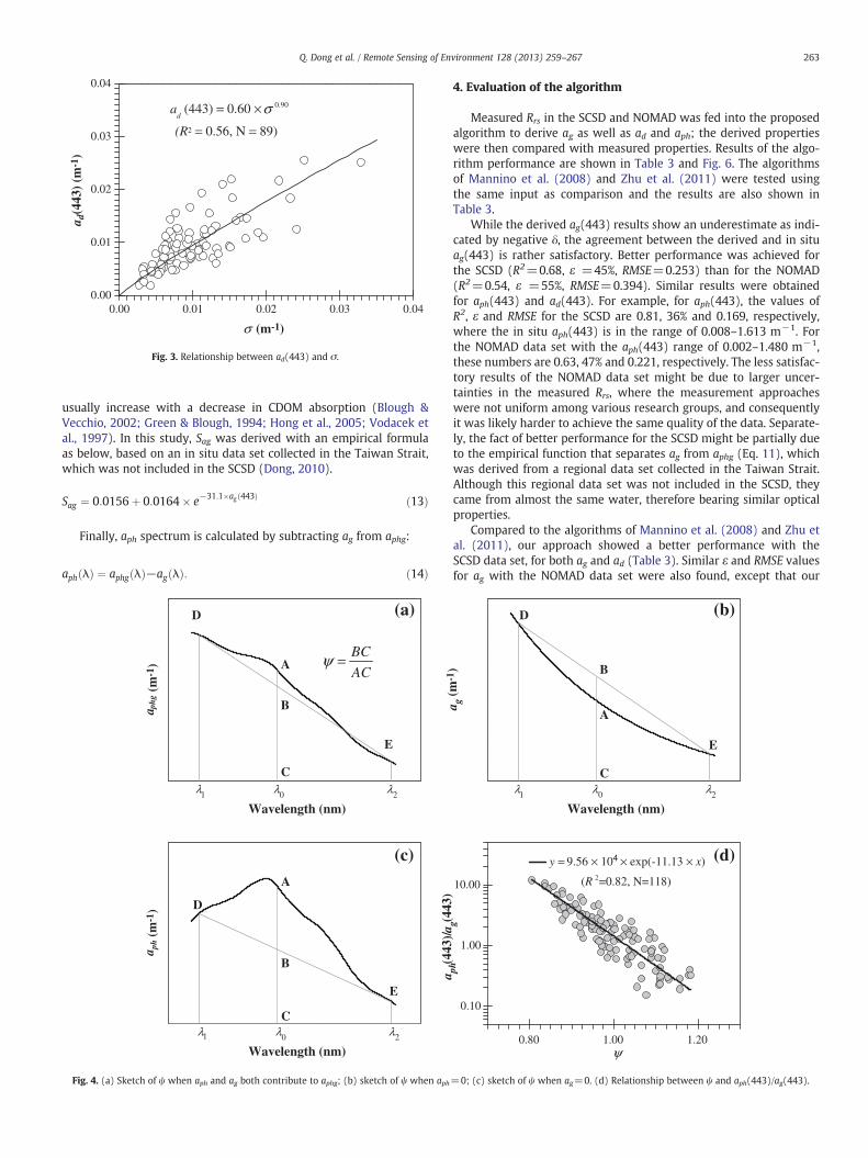
Based on the 89 match-ups of anw(443), bbp(555), Rrs and ad(443)in the NOMAD data set, an empirical relationship to estimate ad(443)was developed through trial and error (R2=0.56, RMSE=0.147,Fig. 3):
Since anw(443) and bbp(555) can be obtained by QAA, σ can be easilycalculated; so can ad(443). Different from earlier approaches (Lee, 1994;Zhu et al., 2011), the above equations estimate ad using three inputs. Forcoastal turbid waters, the ratio of (Rrs(555)+Rrs(670))/Rrs(443) will besignificantly greater than 1.0, then the bbp(555) component plays a biggerrole for the estimation of ad as indicated in earlier studies (Lee, 1994; Zhuet al., 2011). For oceanic waters, (Rrs(555)+Rrs(670))/Rrs(443) could besignificantly smaller than 1.0, then the anw(443) component plays a big-ger role for the ad(443) estimation (Morel, 2009). The combination ofEqs. (7)–(8) thus provides a seamless transition for the estimation of adof coastal and oceanic waters.
The ad spectrum can then be calculated by Eq. (3) if Sad is known.Various Sad values have been reported and its range is relatively narrow(e.g., Roesler et al., 1989). For example, it has an average value of0.011 nm−1 in the Irish Sea (Bowers et al., 1996), and of 0.0123 nm−1
in European coastal waters (Babin et al., 2003). In this study, we use theSad value of 0.012 nm−1, which is an average value of Sad in the TaiwanStrait (Dong, 2010).
3.2. Separation of ag and aph in ocean color inversion
Once ad is obtained, aphg can be derived by subtracting ad from anw:
aphg λð Þ ¼ anw λð Þ−ad λð Þ: ð9Þ
In order to separate ag from aphg, we defined the parameter ψ asthe ratio of the height of a straight line at 443 nm to the height of
ad(λλ)ad(λ0)
Sad
aphg(
anw(λ)
Rrs(λ)QAA
QAA
bbp(λ)
Fig. 2. Schematic flow chart o
aphg(443) (i.e. BC/AC shown in Fig. 4a), where the straight line is de-termined between aphg(412) and aphg(490):
ψ ¼ aphg λ2ð Þaphg λ0ð Þ þ
aphg λ1ð Þ−aphg λ2ð Þaphg λ0ð Þ � λ2−λ0
λ2−λ1;λ1 ¼ 412;λ0 ¼ 443;λ2 ¼ 490:
ð10Þ
Because ag and aph have different spectral characteristics, values ofψ vary with different combinations of ag and aph. For instance, whenaphg has no contribution from aph (i.e., ag alone), ψ will be greaterthan 1.0 (Fig. 4b). On the other hand, when aphg has no contributionfrom ag (i.e., aph alone), ψ will be less than 1.0 (Fig. 4c).
Based on an in situ data set collected in the Taiwan Strait, it is foundthat ψ has a good relationship with the ratio of aph(443)/ag(443) (R2=0.82, N=118; Fig. 4d).
aph 443ð Þ=ag 443ð Þ ¼ 9:56� 104 � e−11:13�ψ ð11Þ
Note that this data set was independent from the SCSD used for al-gorithm assessment, and the measurements of aph and ag followedthe same methods as described in Section 2. Therefore, with givenaphg(443) and aph(443)/ag(443) ratio, ag(443) can be calculated,
We tested this separation approach using the measured aphg data(which are simply the sum of measured aph and ag) in the NOMADand SCSD data sets, and found that it performed very well (Fig. 5).The R2 between calculated and measured properties is 0.97 and0.91, with the RMSE of 0.200 and 0.228, for aph(443) and ag(443), re-spectively, when the scheme was applied to the NOMAD data set. Theresults are 0.98, 0.87, with the RMSE of 0.135 and 0.203, respectively,for the SCSD data set. Because remote sensing platform does not ob-tain aphg directly, the performance of the scheme is not expected tobe as good as that applied to the in situ data set.
With ag(443) derived, the ag spectrum can be calculated by Eq. (2)when Sag is known. The Sag values have a relatively broad range and
aph(λ)ag(λ0)λ) ag(λ)
Sag
f the proposed algorithm.
a d(4
43)
(m-1
)
0.00 0.01 0.02 0.03 0.040.00
0.01
0.02
0.03
0.04
0.90(443) = 0.60 ×d
a
(R2 = 0.56, N = 89)
σ (m-1)
σ
Fig. 3. Relationship between ad(443) and σ.
263Q. Dong et al. / Remote Sensing of Environment 128 (2013) 259–267
usually increase with a decrease in CDOM absorption (Blough &Vecchio, 2002; Green & Blough, 1994; Hong et al., 2005; Vodacek etal., 1997). In this study, Sag was derived with an empirical formulaas below, based on an in situ data set collected in the Taiwan Strait,which was not included in the SCSD (Dong, 2010).
Sag ¼ 0:0156þ 0:0164� e−31:1�ag 443ð Þ ð13Þ
Finally, aph spectrum is calculated by subtracting ag from aphg:
aph λð Þ ¼ aphg λð Þ−ag λð Þ: ð14Þ
a ph
(m-1
)
Wavelength (nm)
a phg
(m
-1)
BC
ACψ =
A
B
C
D
E
A
B
C
E
D
(c)
(a)
Wavelength (nm)0λ 2λ1λ
0λ 2λ1λ
Fig. 4. (a) Sketch of ψ when aph and ag both contribute to aphg; (b) sketch of ψ when aph
4. Evaluation of the algorithm
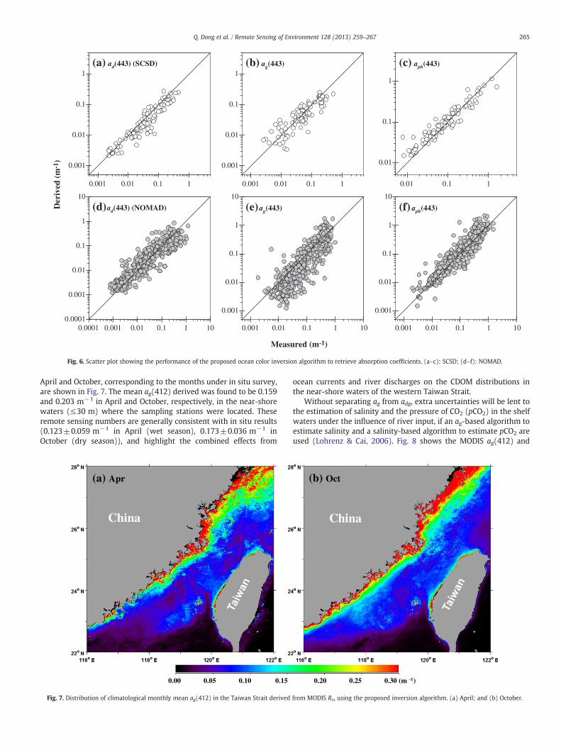
Measured Rrs in the SCSD and NOMAD was fed into the proposedalgorithm to derive ag as well as ad and aph; the derived propertieswere then compared with measured properties. Results of the algo-rithm performance are shown in Table 3 and Fig. 6. The algorithmsof Mannino et al. (2008) and Zhu et al. (2011) were tested usingthe same input as comparison and the results are also shown inTable 3.
While the derived ag(443) results show an underestimate as indi-cated by negative δ, the agreement between the derived and in situag(443) is rather satisfactory. Better performance was achieved forthe SCSD (R2=0.68, ε =45%, RMSE=0.253) than for the NOMAD(R2=0.54, ε =55%, RMSE=0.394). Similar results were obtainedfor aph(443) and ad(443). For example, for aph(443), the values ofR2, ε and RMSE for the SCSD are 0.81, 36% and 0.169, respectively,where the in situ aph(443) is in the range of 0.008–1.613 m−1. Forthe NOMAD data set with the aph(443) range of 0.002–1.480 m−1,these numbers are 0.63, 47% and 0.221, respectively. The less satisfac-tory results of the NOMAD data set might be due to larger uncer-tainties in the measured Rrs, where the measurement approacheswere not uniform among various research groups, and consequentlyit was likely harder to achieve the same quality of the data. Separate-ly, the fact of better performance for the SCSD might be partially dueto the empirical function that separates ag from aphg (Eq. 11), whichwas derived from a regional data set collected in the Taiwan Strait.Although this regional data set was not included in the SCSD, theycame from almost the same water, therefore bearing similar opticalproperties.
Compared to the algorithms of Mannino et al. (2008) and Zhu etal. (2011), our approach showed a better performance with theSCSD data set, for both ag and ad (Table 3). Similar ε and RMSE valuesfor ag with the NOMAD data set were also found, except that our
0.80 1.00 1.20
a ph(4
43)/ a
g(44
3)
0.10
1.00
10.002
9.56 × 10⁴ × exp(-11.13 × x)
=0.82, N=118)
y
(R
= (d)
Wavelength (nm)
a g (m
-1)
A
B
C
D
E
(b)
ψ
0λ 2λ1λ
=0; (c) sketch of ψ when ag=0. (d) Relationship between ψ and aph(443)/ag(443).
Mod
el r
esul
ts (
m-1
)
0.001
0.01
0.1
1
0.001
0.01
0.1
1
Measured (m-1)
0.001
0.01
0.1
1
0.001 0.01 0.1 1 0.001 0.01 0.1 1
0.001 0.01 0.1 10.001 0.01 0.1 1
0.001
0.01
0.1
1
(d) aph(443) (NOMAD)
(a) ag(443) (SCSD)
(c) ag(443) (NOMAD)
(b) aph(443) (SCSD)
Fig. 5. (a and c) Measured ag versus modeled ag, which is partitioned from aphg based on Eqs (10)–(13). (b and d) Measured aph versus modeled aph partitioned from aphg using Eq. (14).
264 Q. Dong et al. / Remote Sensing of Environment 128 (2013) 259–267
approach resulted in more serious underestimate of ag(443). Howev-er, we noticed that the ad(443) produced with the approach of Zhu etal. (2011) was deviated seriously from the observed ad(443), while εand δ were 84% and −0.716, respectively. This indicates that using acombination of bbp, anw, and Rrs to derive ad, which was one of the key
Table 3Error statistics between derived and in situ absorption coefficients.
N is the number of data tested, while n is the number of valid retrievals. ag1 and ad1 were
derived using the approach of Zhu et al. (2011); ag2 was derived using the approach ofMannino et al. (2008).
elements of the proposed algorithm in this study, was more adequatethan the approaches that simply employ bbp alone (Lee, 1994; Zhu etal., 2011). It is also noticeable that there were 172 invalid retrievalswhen using the empirical algorithmofMannino et al. (2008). Of course,part of the less satisfied performance of the above two regional algo-rithms may be arisen from the fact that the empirical coefficients inthe algorithms were not tuned using data included in this study.
The above results are encouraging because ag, as an important bio-geochemical property, is nearly analytically derived from ocean colormeasurements. This approach is likely applicable to global waters,although tests with more data are certainly needed.
5. Implications
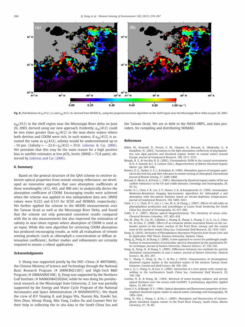
Our results demonstrate that ag can be analytically derived fromremote sensing reflectance in both coastal and oceanic waters. Thisis especially significant for a better understanding of the biogeochem-istry of coastal systems using satellite data. We previously reportedseasonal variations of ag(412) based on field measurements in thenear-shore waters of the Taiwan Strait (Du et al., 2010). In the presentwork, we produced climatological monthly mean ag(412) of this re-gion using MODIS Rrs (version R2005.1, period of 2003–2008) as theinput, based on the assumption that the default atmospheric correc-tion approach (Gordon & Wang, 1994) was applicable to this region.The reason to produce climatological monthly mean numbers is thatthere were no applicable MODIS Rrs data during the cruise time(4–5 days) owing to serious influences of clouds and sun glints. Togenerate climatological monthly mean ag(412), daily ag(412) wasfirst derived by feeding Level 2 daily Rrs of 1 km resolution (http://oceancolor.gsfc.nasa.gov/) into the proposed algorithm. Results in
Fig. 6. Scatter plot showing the performance of the proposed ocean color inversion algorithm to retrieve absorption coefficients. (a–c): SCSD; (d–f): NOMAD.
265Q. Dong et al. / Remote Sensing of Environment 128 (2013) 259–267
April and October, corresponding to the months under in situ survey,are shown in Fig. 7. The mean ag(412) derived was found to be 0.159and 0.203 m−1 in April and October, respectively, in the near-shorewaters (≤30 m) where the sampling stations were located. Theseremote sensing numbers are generally consistent with in situ results(0.123±0.059 m−1 in April (wet season), 0.173±0.036 m−1 inOctober (dry season)), and highlight the combined effects from
0.00 0.05 0.150.10
(a) Apr
China
Fig. 7. Distribution of climatological monthly mean ag(412) in the Taiwan Strait derived
ocean currents and river discharges on the CDOM distributions inthe near-shore waters of the western Taiwan Strait.
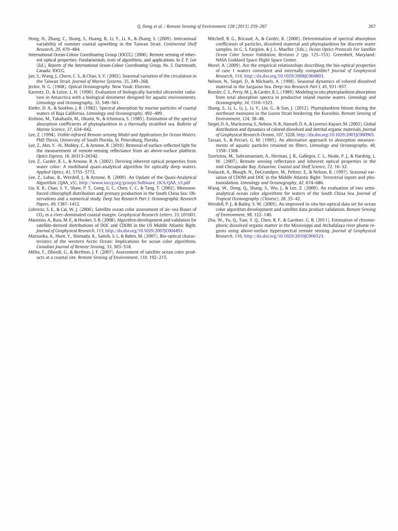
Without separating ag from adg, extra uncertainties will be lent tothe estimation of salinity and the pressure of CO2 (pCO2) in the shelfwaters under the influence of river input, if an ag-based algorithm toestimate salinity and a salinity-based algorithm to estimate pCO2 areused (Lohrenz & Cai, 2006). Fig. 8 shows the MODIS ag(412) and
0.20 0.25 0.30 (m -1)
(b) Oct
China
from MODIS Rrs using the proposed inversion algorithm. (a) April; and (b) October.
(a) (b)
0.00 0.20 0.800.600.40 1.00 (m -1)
Fig. 8. Distributions of ag(412) (a) and adg(412) (b) derived fromMODIS Rrs using the proposed inversion algorithm on the shelf region near the Mississippi River delta on June 26, 2003.
266 Q. Dong et al. / Remote Sensing of Environment 128 (2013) 259–267
adg(412) in the shelf region near the Mississippi River delta on June26, 2003, derived using our new approach. Evidently, adg(412) couldbe two times greater than ag(412) in the near-shore waters whereboth detritus and CDOM were rich. In such waters, if adg(412) is as-sumed the same as ag(412), salinity would be underestimated up to~10 psu (Salinity=−22.4×ag(412)+35.0; Lohrenz & Cai, 2006).We postulate that this may be the main reason for a high positivebias in satellite estimates at low pCO2 levels (RMSE=72.8 μatm) ob-served by Lohrenz and Cai (2006).
6. Summary
Based on the general structure of the QAA scheme to retrieve in-herent optical properties from remote sensing reflectance, we devel-oped an innovative approach that uses absorption coefficients atthree wavelengths (412, 443, and 490 nm) to analytically derive theabsorption coefficient of CDOM. Encouraging results were achievedwhen the scheme was applied to two independent data sets (RMSEvalues were 0.222 and 0.315 for SCSD and NOMAD, respectively).We further applied the scheme to the MODIS measurements overthe Taiwan Strait as well as the Mississippi River Delta, and foundthat the scheme not only generated consistent results comparedwith the in situ measurements but also improved the estimation ofsalinity in near-shore regions where absorption of CDOM is used asan input. While this new algorithm for retrieving CDOM absorptionhas produced encouraging results, as with all evaluations of remotesensing products (such as chlorophyll a concentration or diffuse at-tenuation coefficient), further studies and refinements are certainlyrequired to ensure a robust application.
Acknowledgments
S. Shang was supported jointly by the NSF—China (# 40976068),the Chinese Ministry of Science and Technology through the NationalBasic Research Program (# 2009CB421201) and High-Tech R&DProgram (# 2008AA09Z108). Q. Dong was supported by the NorthernGulf Institute (# NA06OAR4320264) while he was doing his postdoc-toral research at the Mississippi State University. Z. Lee was partiallysupported by the Energy and Water Cycle Program of the NationalAeronautics and Space Administration (# NNX09AV97G). We thankthe crew of R/V Yanping II, and Jingyu Wu, Xiaoxin Ma, Xiaofei Sui,Wen Zhou, Wenqi Wang, Min Yang, Cuifen Du and Guomei Wei fortheir help in collecting the in situ data in the South China Sea and
the Taiwan Strait. We are in debt to the NASA-OBPG, and data pro-viders, for compiling and distributing NOMAD.
References
Babin, M., Stramski, D., Ferrari, G. M., Claustre, H., Bricaud, A., Obolensky, G., &Hoepffner, N. (2003). Variations in the light absorption coefficients of phytoplank-ton, non algal particles and dissolved organic matter in coastal waters aroundEurope. Journal of Geophysical Research, 108, 3211–3231.
Blough, N. V., & Vecchio, R. D. (2002). Chromophoric DOM in the coastal environment.In D. A. Hansell, & C. A. Carlson (Eds.), Biogeochemistry of Marine Dissolved OrganicMatter (pp. 509–546).
Bowers, D. G., Harker, G. E. L., & Stephan, B. (1996). Absorption spectra of inorganic parti-cles in the Irish Sea and their relevance to remote sensing of chlorophyll. InternationalJournal of Remote Sensing, 17, 2449–2460.
Bricaud, A., Morel, A., & Prieur, L. (1981). Absorption by dissolved organicmatter of the sea(yellow Substance) in the UV and visible domains. Limnology and Oceanography, 26,43–53.
Carder, K. L., Chen, F. R., Lee, Z. P., Hawes, S. K., & Kamykowski, D. (1999). SemianalyticModerate-Resolution Imaging Spectrometer algorithms for chlorophyll a andabsorption with bio-optical domains based on nitrate-depletion temperatures.Journal of Geophysical Research, 104, 5403–5421.
Chen, Y. L. L., Chen, H. Y., Lin, I. I., Lee, M. A., & Chang, J. (2007). Effects of cold eddy onphytoplankton production and assemblages in Luzon Strait bordering the SouthChina Sea. Journal of Oceanography, 63, 671–683.
Coble, P. G. (2007). Marine optical biogeochemistry: The chemistry of ocean color.Chemical Reviews-Columbus, 107, 402–418.
Dai, M., Zhai, W., Cai, W., Callahan, J., Huang, B., Shang, S., Huang, T., Li, X., Lu, Z., Chen,W., & Chen, Z. (2008). Effects of an estuarine plume-associated bloom on the car-bonate system in the lower reaches of the Pearl River estuary and the coastalzone of the northern South China Sea. Continental Shelf Research, 28, 1416–1423.
Dong, Q. (2010). Derivation of Phytoplankton Absorption Properties from Ocean Color andIts Application. PhD Thesis, Xiamen University, Xiamen, China.
Dong, Q., Hong, H., & Shang, S. (2008). A new approach to correct for pathlength ampli-fication in measurements of particulate spectral absorption by the quantitative fil-ter technique. Journal of Xiamen University (Natural Science), 47, 556–561.
Dong, Q., Hong, H., & Shang, S. (2009). Differences between two methods for particleabsorption measurements in case-2 waters. Journal of Xiamen University (NaturalScience), 48, 293–297.
Du, C., Shang, S., Dong, Q., Hu, C., & Wu, J. (2010). Characteristics of chromophoricdissolved organic matter in the nearshore waters of the western Taiwan Strait.Estuarine, Coastal and Shelf Science, 88, 350–356.
Gan, J., Li, L., Wang, D., & Guo, X. (2009). Interaction of a river plume with coastal up-welling in the northeastern South China Sea. Continental Shelf Research, 29,728–740.
Gordon, H. R., & Wang, M. (1994). Retrieval of water-leaving radiance and aerosoloptical thickness over the oceans with SeaWiFS: A preliminary algorithm. AppliedOptics, 33, 443–452.
Green, S. A., & Blough, N. V. (1994). Optical absorption and fluorescence properties of chro-mophoric dissolved organic matter in natural waters. Limnology and Oceanography, 39,1903–1916.
Hong, H., Wu, J., Shang, S., & Hu, C. (2005). Absorption and fluorescence of chromo-phoric dissolved organic matter in the Pearl River Estuary, South China. MarineChemistry, 97, 78–89.
267Q. Dong et al. / Remote Sensing of Environment 128 (2013) 259–267
Hong, H., Zhang, C., Shang, S., Huang, B., Li, Y., Li, X., & Zhang, S. (2009). Interannualvariability of summer coastal upwelling in the Taiwan Strait. Continental ShelfResearch, 29, 479–484.
International Ocean-Colour Coordinating Group (IOCCG) (2006). Remote sensing of inher-ent optical properties: Fundamentals, tests of algorithms, and applications. In Z. P. Lee(Ed.), Reports of the International Ocean-Colour Coordinating Group, No. 5. Dartmouth,Canada: IOCCG.
Jan, S., Wang, J., Chern, C. S., & Chao, S. Y. (2002). Seasonal variation of the circulation inthe Taiwan Strait. Journal of Marine Systems, 35, 249–268.
Jerlov, N. G. (1968). Optical Oceanography. New Youk: Elsevier.Karentz, D., & Lutze, L. H. (1990). Evaluation of biologically harmful ultraviolet radia-
tion in Antarctica with a biological dosimeter designed for aquatic environments.Limnology and Oceanography, 35, 549–561.
Kiefer, D. A., & SooHoo, J. B. (1982). Spectral absorption by marine particles of coastalwaters of Baja California. Limnology and Oceanography, 492–499.
Kishino, M., Takahashi, M., Okami, N., & Ichimura, S. (1985). Estimation of the spectralabsorption coefficients of phytoplankton in a thermally stratified sea. Bulletin ofMarine Science, 37, 634–642.
Lee, Z. (1994). Visible-infrared Remote-sensing Model and Applications for Ocean Waters.PhD Thesis, University of South Florida, St. Petersburg, Florida.
Lee, Z., Ahn, Y. -H., Mobley, C., & Arnone, R. (2010). Removal of surface-reflected light forthe measurement of remote-sensing reflectance from an above-surface platform.Optics Express, 18, 26313–26342.
Lee, Z., Carder, K. L., & Arnone, R. A. (2002). Deriving inherent optical properties fromwater color: A multiband quasi-analytical algorithm for optically deep waters.Applied Optics, 41, 5755–5772.
Lee, Z., Lubac, B., Werdell, J., & Arnone, R. (2009). An Update of the Quasi-AnalyticalAlgorithm (QAA_v5). http://www.ioccg.org/groups/Software_OCA/QAA_v5.pdf
Liu, K. K., Chao, S. Y., Shaw, P. T., Gong, G. C., Chen, C. C., & Tang, T. (2002). Monsoon-forced chlorophyll distribution and primary production in the South China Sea: Ob-servations and a numerical study. Deep Sea Research Part I: Oceanographic ResearchPapers, 49, 1387–1412.
Lohrenz, S. E., & Cai, W. J. (2006). Satellite ocean color assessment of air–sea fluxes ofCO2 in a river-dominated coastal margin. Geophysical Research Letters, 33, L01601.
Mannino, A., Russ,M. E., & Hooker, S. B. (2008). Algorithmdevelopment and validation forsatellite-derived distributions of DOC and CDOM in the US Middle Atlantic Bight.Journal of Geophysical Research, 113, http://dx.doi.org/10.1029/2007JC004493.
Matsuoka, A., Huot, Y., Shimada, K., Saitoh, S. I., & Babin, M. (2007). Bio-optical charac-teristics of the western Arctic Ocean: Implications for ocean color algorithms.Canadian Journal of Remote Sensing, 33, 503–518.
Mélin, F., Zibordi, G., & Berthon, J. F. (2007). Assessment of satellite ocean color prod-ucts at a coastal site. Remote Sensing of Environment, 110, 192–215.
Mitchell, B. G., Bricaud, A., & Carder, K. (2000). Determination of spectral absorptioncoefficients of particles, dissolved material and phytoplankton for discrete watersamples. In G. S. Fargion, & J. L. Mueller (Eds.), Ocean Optics Protocols For SatelliteOcean Color Sensor Validation, Revision 2 (pp. 125–153). Greenbelt, Maryland:NASA Goddard Space Flight Space Center.
Morel, A. (2009). Are the empirical relationships describing the bio-optical propertiesof case 1 waters consistent and internally compatible? Journal of GeophysicalResearch, 114, http://dx.doi.org/10.1029/2008JC004803.
Nelson, N., Siegel, D., & Michaels, A. (1998). Seasonal dynamics of colored dissolvedmaterial in the Sargasso Sea. Deep-Sea Research Part I, 45, 931–957.
Roesler, C. S., Perry,M. J., & Carder, K. L. (1989).Modeling in situ phytoplankton absorptionfrom total absorption spectra in productive inland marine waters. Limnology andOceanography, 34, 1510–1523.
Shang, S., Li, L., Li, J., Li, Y., Lin, G., & Sun, J. (2012). Phytoplankton bloom during thenortheast monsoon in the Luzon Strait bordering the Kuroshio. Remote Sensing ofEnvironment, 124, 38–48.
Siegel, D. A.,Maritorena, S., Nelson, N. B., Hansell, D. A., & Lorenzi-Kayser,M. (2002). Globaldistribution and dynamics of colored dissolved and detrital organic materials. Journalof Geophysical Research-Oceans, 107, 3228, http://dx.doi.org/10.1029/2001JC000965.
Tassan, S., & Ferrari, G. M. (1995). An alternative approach to absorption measure-ments of aquatic particles retained on filters. Limnology and Oceanography, 40,1358–1368.
Tzortziou, M., Subramaniam, A., Herman, J. R., Gallegos, C. L., Neale, P. J., & Harding, L.W. (2007). Remote sensing reflectance and inherent optical properties in themid Chesapeake Bay. Estuarine, Coastal and Shelf Science, 72, 16–32.
Vodacek, A., Blough, N., DeGrandpre, M., Peltzer, E., & Nelson, R. (1997). Seasonal var-iation of CDOM and DOC in the Middle Atlantic Bight: Terrestrial inputs and pho-tooxidation. Limnology and Oceanography, 42, 674–686.
Wang, W., Dong, Q., Shang, S., Wu, J., & Lee, Z. (2009). An evaluation of two semi-analytical ocean color algorithms for waters of the South China Sea. Journal ofTropical Oceanography (Chinese), 28, 35–42.
Werdell, P. J., & Bailey, S. W. (2005). An improved in-situ bio-optical data set for oceancolor algorithm development and satellite data product validation. Remote Sensingof Environment, 98, 122–140.
Zhu, W., Yu, Q., Tian, Y. Q., Chen, R. F., & Gardner, G. B. (2011). Estimation of chromo-phoric dissolved organic matter in the Mississippi and Atchafalaya river plume re-gions using above-surface hyperspectral remote sensing. Journal of GeophysicalResearch, 116, http://dx.doi.org/10.1029/2010JC006523.