The Occultation Radiometer ~ORA! developed bythe Belgian Institute for Space Aeronomy is a sim-ple UV–visible instrument that was launched inJuly 1992 onboard the European Retrievable Carrier~EURECA! for a 1-year mission. The instrumentwas dedicated to the measurement of vertical profilesof O3, NO2, and H2O number densities as well as ofstratospheric aerosols.
Using the well-known method of solar occultationthrough the Earth’s atmosphere, the ORA recorded;7000 sunsets and sunrises from a circular orbit atan altitude of 508 km. Although the low orbitalplane inclination ~28°! of the satellite restricted thelatitude coverage to 40 °S and 40 °N, the period ofmeasurement was particularly interesting because itpresented a unique opportunity for observing the re-laxation of the Pinatubo eruptive perturbations.
The experimental design has been described else-where.1 Briefly, it consists of eight broadband chan-nels whose nominal wavelengths are presented inTable 1 together with the associated predominantconstituents.
The authors are with the Institut d’Aeronomie Spatiale de Bel-gique, 3 avenue Circulaire, B 1180 Brussels, Belgium. The e-mailaddress for D. Fussen is [email protected].
Received 23 November 1999; revised manuscript received 10October 2000.
A major characteristic of the ORA is its simpleoptics that has a 62° field of view and is aligned withthe Sun-tracking system of the satellite. As a con-sequence, the apparent vertical resolution of the in-strument appears to be poor ~;25 km, defined by thesize of the solar disk at the tangent point!. Howeverthe signal-to-noise ratio was high for the same rea-son, suggesting that a large amount of informationcan be retrieved from the transmission and permit-ting the achievement of a 2–3-km vertical resolution.
In this paper we present the final inversion algo-rithm of the ORA experiment. In Section 2 we de-scribe the improvements made to the alreadydeveloped vertical inversion scheme. Then we dis-cuss the spectral inversion ~or separation among thearious constituents! as well as the error budget.inally, we compare the inverted ORA profiles withhose obtained by the Stratospheric Aerosol and Gasxperiment II ~SAGE II!.2,3
2. Vertical Inversion Algorithm
The retrieval of constituent altitude profiles faces twoinversion problems: For vertical inversion, one hasto compute the relative contribution of each atmo-spheric layer to the slant path’s optical thickness; forspectral inversion, one separates different speciesthat absorb light at the same wavelength. The un-usual choice of performing the vertical inversion be-fore the spectral inversion was motivated by our needto solve the more difficult problem first. Further-more, the wavelength dependence of aerosol extinc-tion is unknown but varies a priori with altitude.
20 February 2001 y Vol. 40, No. 6 y APPLIED OPTICS 941
ts
v
st
T
v
1cttproiabprc
evtf
tmma
o
Table 1. Major Light Absorbers for the ORA Channels
9
Performing the spectral inversion first permits onlyaveraged values that correspond to a particular tan-gent altitude to be obtained. In the vertical inver-sion, the atmospheric extinction coefficient isintegrated along the line of sight but also over thesolid angle spanned by the apparent solar disk.When the refractive effects and solar limb darkeningare taken into account, the inversion problem of re-trieving the vertical extinction profile becomes quitecomplicated and is highly nonlinear. There arewell-known published algorithms for addressing theproblem of inverting a slant path’s optical thick-nesses recorded during a solar occultation. Theclassic onion-peeling method is clearly inadequatebecause of the collective contribution of a large alti-tude range to the signal. The Chahine algorithmused in the SAGE II ~Ref. 2! was also tested butturned out to become unstable ~wavy spurious struc-tures appeared! beyond an optimal number of itera-ions that is difficult to determine a priori and isomewhat arbitrary. Optimal estimation methods,4
were also considered, but the effects of the high non-linearity of the problem in a Bayesian approach wereexpected to perturb the error analysis that is a majoradvantage of this formalism. Also, the absence ofvalidated climatologies related to the covariance ma-trix of the altitude profiles of the aerosol extinctionwas judged to be a large uncertainty factor inhibitingdefinition of the a priori state vector after a majorolcanic eruption.In an earlier publication,5 the Natural Orthogonal
Polynomial Expansion ~NOPE! method was pre-ented as a useful tool for describing the total extinc-ion profile b~z! ~expressed in units of inverse meters!
b~z! 5 b0~z! (i50
n
aiPi~z!, (1)
where b0~z! stands for a reasonable a priori profile.he family of orthogonal polynomials Pi~z! was nu-
merically generated by the Stieltjes procedure. Fi-nally, a merit function that compared the squareddifference between the modeled and the observedtransmissions was minimized with respect to the aicoefficients, by use of a Levenberg–Marquardt algo-rithm.
In a recent publication6 the whole algorithm wasalidated by comparison of ;25 coincident ORA and
SAGE II ~Ref. 2! total extinction profiles for three
42 APPLIED OPTICS y Vol. 40, No. 6 y 20 February 2001
common spectral channels ~l 5 385, 600, 1020 nm!.The agreement was acceptable ~typically 20% in the
5–40-km altitude range!, proving that the methodan be used to retrieve small- to medium-scale ver-ical structures ~2–5 km! that are much smallerhan the Sun’s apparent size. However, the ORArofiles turned out to be slightly oversmoothed withespect to the SAGE because they are constructedn the basis of continuous functions. A second lim-tation of the method was the intermittent appear-nce of a more chaotic profile behavior above 35 andelow 15 km, where the transmission signal ap-roaches 1 ~small optical thickness! or 0 ~saturationegime!. The problem was clearly identified asancellation effects in the ai coefficients enhanced
by the important redundancy between two trans-missions recorded at two neighboring tangent alti-tudes ~for which there is a large overlap betweenthe corresponding apparent solar disks!. How-ver, increasing the size n ~which normally has thealue of 10! of the basis was inefficient because ofhe complicated and flat topology about the meritunction minimum.
Preliminary spectral inversion of the retrieved to-al extinction profiles showed, in the altitude rangeentioned, the high sensitivity of the results to theore chaotic part of the extinction profile. Looking
t the residual ~typically 2 3 1023! of the merit func-tion, however, clearly showed that this residual wasan oscillating but smooth function of altitude, wellabove the noise level of the instrument. As no moreinformation could be extracted from the inversion ofone occultation by the NOPE method, we decided toincrease the information content by using a largesubset of inverted profiles to construct a geometricdirect method ~DM! that would be capable of produc-ing more-robust profiles in the low- and high-altituderegions.
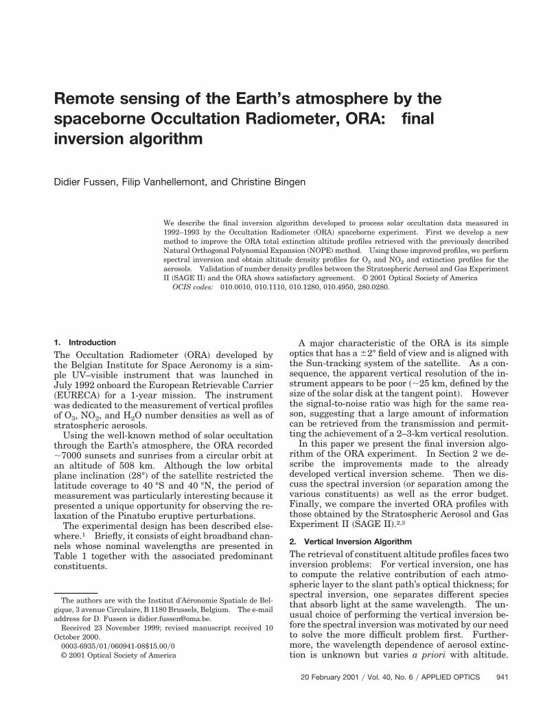
In Fig. 1 we present a schematic view of the occul-tation geometry. It is clear that the main contribu-tion to the slant-path optical thickness comes from a
Fig. 1. Measured transmittance ~inset! is a smooth function of thetangent altitude. At satellite position 2, the signal is influencedmainly by the atmospheric layers that define the Sun’s apparentsize ~z 5 hmin to z 5 hmax!. Note that we use h for the tangentaltitude, which varies during the occultation, and z for the altitudeat which the profile is computed. Reciprocally, the value of theextinction coefficient at z 5 h is strongly determined by the valuef the transmittance recorded between satellite positions 1 and 3.
stiaa
t
Utttdmo
limited region of length S ~;500 km for Rayleighcattering! surrounding the tangent point. Theransmitted signal at satellite position 2 is thereforenfluenced mainly by the value of the total extinctiont z 5 h and also by all rays that issue from theltitudes that range approximately from hmin to hmax.
It is natural to consider that the value of the totalextinction at z 5 h can be formally determined fromthe evolution of the total transmission betweenpoints 1 and 3. Using a scale factor ~S 5 500 km! forhe optical path, we express b~z! as
b~z! 52ln~y!
S1 bmin
R ~z!, (2)
where
y 5 y~z! 5 $tanh@z~z! 2 1y2# 1 1%y2, (3)
z~z! 5 *hmin~ z!
hmax~ z!
f ~h; z!T~h!dh, (4)
where f ~h; z! is an unknown function that weights themeasured transmittance T~h! along the nominal tan-gent altitude h. Equation ~4! defines z~z! as aweighted sum of the transmission values that con-tribute to the value of b~z!. The nonlinear transfor-mation of Eq. ~3! has the property of constraining theeffective transmission y~z! to range from 0 to 1. ForEq. ~2! we decided to constrain the total extinctioncoefficient to be greater than or equal to a minimalvalue acceptable for the Rayleigh extinction coeffi-cient. Considerations about the natural variabilityof air density led us to choose
bminR ~z! 5 0.9b0
R~z! ~z # 30 km!
5 @0.9 2 0.01~z 2 30!#b0R~z! ~30 km , z
# 50 km!, (5)
where b0R~z! is the Rayleigh extinction profile for the
.S. 1976 Standard Atmosphere. We believe thathis piecewise linear profile is a good approximationo a lower bound of the climatological Rayleigh scat-ering ~this means that the DM cannot be used toescribe total extinction profiles that lie below thisinimal profile!. Finally, we introduce the change
f variable
x~h! 5@h 2 hmin~z!#
Dh2 1 HDh ;
@hmax~z! 2 hmin~z!#
2 J .
(6)
We obtain
z~z! 5 *21
1
f @h~x!; z#T@h~x!#dx. (7)
The weighting function f @h~x!; z# is developed, for anyaltitude z, on the basis of the first eleven Chebyshevpolynomials as
f ~x, z! 5 (j50
10
aj~z!cos@ j arccos~x!#. (8)
After algebraic inversion of Eqs. ~2!–~4!, the aj~z! co-efficients were determined by use of a linear least-squares procedure with the results of 1000occultations that had been vertically inverted by theNOPE method, and the error in b~z! was estimatedfrom the associated covariance matrix and standarderror propagation ~the ORA error characterizationhas been discussed in Ref. 6!. The DM is in fact anonlinear mapping between transmission curves andextinction profiles. It presupposes that the effec-tive inversion scheme is determined only by theoccultation geometry, which does not vary with time.However, we used the refracted rays produced by aray-tracing computation to determine hmin~z! andhmax~z!.
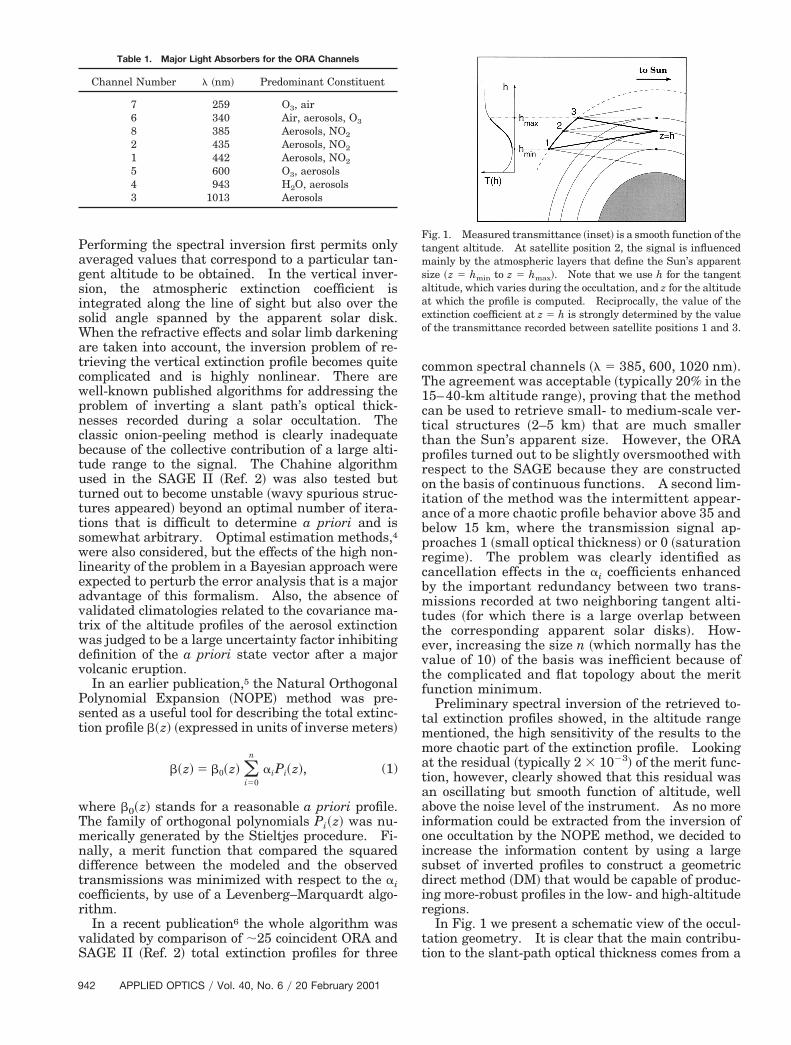
In Fig. 2 we present a typical result of both theNOPE method and the DM. In the upper part of thefigure the NOPE total extinction profiles at l 5 600nm and l 5 1013 nm are represented by circles. Atl 5 1013 nm, some erratic behavior occurs above 40km. Note, however, the large dynamic range of theprofile. In the lower part of the figure the associatedbest-fit transmission is plotted relative to the mea-sured transmission. A close examination revealsthat the modeled transmission in the NOPE methoddoes not perfectly fit the dip at 15 km associated withthe Junge layer maximum at 20 km. Below 5 km,the NOPE transmission seems to be slightly overes-timated. All these effects seem to have been ame-liorated by the application of the DM. Also, at l 5600 nm, we observe a very good fit between measure-ment and NOPE modeled transmission in the rangefrom 20 to 40 km. The DM does not introduce a
Fig. 2. Top, NOPE total extinction ~circles! and corrected DMprofiles ~solid curves!. Dashed curves, Rayleigh extinction. Bot-tom, Measured transmission ~solid curves! and modeled NOPEtransmission ~circles!.
20 February 2001 y Vol. 40, No. 6 y APPLIED OPTICS 943
wc
senotu
1aKwn
r
9
large correction at these altitudes, as we would ex-pect for consistency. Below 20 km, where the trans-mission is almost zero, the total extinction receivesextra stabilization. It is worth noting that the re-sults of the DM are independently computed for eachevent and for each altitude from the raw normalizedtransmission even if the coefficients used, aj~z!, weredetermined by use of a large number of statistics ofoccultations.
Finally, it is interesting to evaluate the verticalresolution of the ORA instrument. A good descrip-tion of the error analysis formalism may be found inRef. 7, where the matrix of averaging kernels F re-lates the a priori profile b0~z!, the retrieved profileb~z!, and the true profile bt~z! through the relation
@b~z! 2 b0~z!# 5 F@bt~z! 2 b0~z!#. (9)
At a given altitude, the averaging kernel is repre-sented by the corresponding row of F. However, F isnot guaranteed to be positive, and negative lobes mayappear that make the interpretation of vertical reso-lution difficult. Such was the case for the ORA,probably because of the nonlinearities of both themeasured signal and inversion methods. Instead,we decided to rewrite Eq. ~9! as
@b~z! 2 b0~z!# 5 *0
`
f~z9!@bt~z9! 2 b0~z9!#dz9, (10)
where the kernel function f is constrained to be pos-itive by the choice of
f~z9! 5g
dÎpexpF2Sz9 2 zp
d D2G , (11)
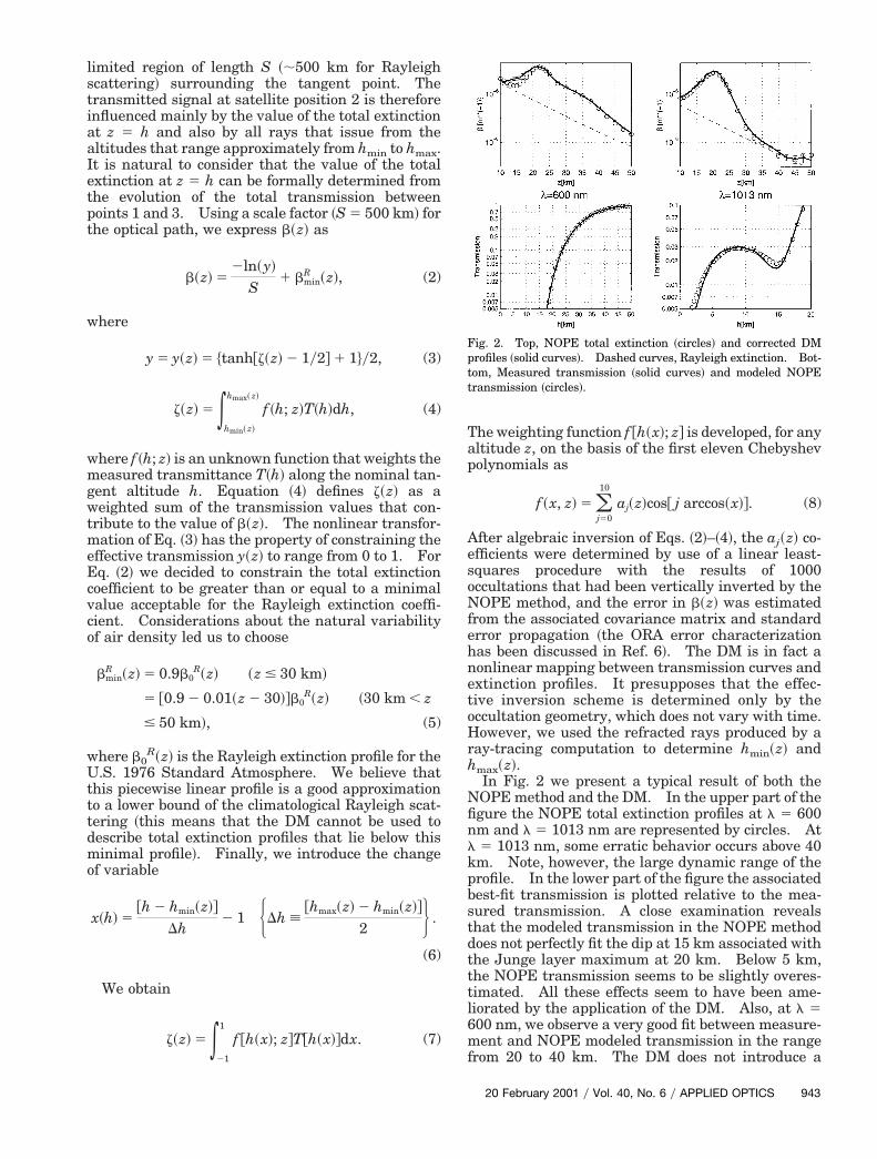
and g, zp, and d are undetermined constants. Ateach altitude z, Eq. ~10! has been numerically solvedin a least-squares sense with respect to g, zp, and d fora large number of input and retrieved profiles inchannel 5 ~l 5 600 nm!. In Fig. 3, we present thevalue of d~z!, showing a good indication of the ORA
Fig. 3. Left, centroid ~zp! of the averaging kernel; right, verticalesolution d~z!.
44 APPLIED OPTICS y Vol. 40, No. 6 y 20 February 2001
vertical resolution, which is ;2 km except below 20km where it increases to 5 km. In the same figurewe have also plotted zp~z!, which indicates that theaveraging kernel above 40 km is influenced mainly bythe lower edge of the Sun.
3. Spectral Inversion Algorithm
In considering the acceptable quality of the verticalinversion, we restrict the spectral inversion to the 26U.S. Standard Atmosphere layers at zi 5 10,11, . . . 25, 27.5, . . . 50 km and, for the time being, wediscard channel 7 ~l 5 259 nm!, which turned out tobe defective, and channel 4 ~l 5 943 nm!, where
ater absorption requires a specific line-by-line cal-ulation.
A common problem that one encounters in thepectral inversion of UV–visible data is the interfer-nce of absorbing constituents that do not exhibit aoticeably structured wavelength dependence. Inther words, the measurement channels are not spec-rally independent, and an example of an extremelynfavorable case would be a l24 aerosol dependence,
making the aerosol contribution indistinguishablefrom Rayleigh scattering by air. Therefore we de-cided to remove the air density by using assimilateddata computed by the United Kingdom Meteorologi-cal Office and suitably interpolated at the ORA tan-gent point ~the estimated error grows roughlylinearly from 1% at 20 km to 2.5% at 50 km!.
Considering the set of total extinction coefficientsat altitude zi, one can write a system of linear equa-tions that relate the extinction by O3, NO2, and aero-sols in the ORA channels as
3R6
N R6O 1 0 0 0 0 0
R8N R8
O 0 1 0 0 0 01 R2
O 0 0 1 0 0 0R1
N R1O 0 0 0 1 0 0
R5N 1 0 0 0 0 1 0
R3N R3
O 0 0 0 0 0 1
43b2
N
b5O
b6A
b8A
b2A
b1A
b5A
b3A
4 5 3b6
b8
b2
b1
b5
b3
4 , (12)
or, in matrix form,
Ai z xi 5 bi, (13)
where RjN 5 sj
Nys2N, Rj
O 5 sjOys5
O, and sjN and sj
O
refer to photoabsorption cross sections by, respec-tively, NO2 and O3 in channel j after convolution withthe instrument function and bj
A stands for the aero-sol extinction coefficient in channel j.
The aerosol wavelength dependence is a product ofthe spectral inversion, unlike in absorption cross sec-tions for O3 and NO2, which are measured in thelaboratory. By simultaneously retrieving O3 andNO2, the six available measurement channels $6, 8, 2,, 5, 3% allow for four degrees of freedom for aerosol,nd this leads to exaggerated noise sensitivity.eeping in mind, however, that broad extrema in theavelength dependence were observed after the Pi-atubo eruption, we decided to describe the spectral
gtaOte
c
a
behavior of the aerosol extinction coefficient in chan-nel j as
bjA~l! 5 c0 1 c1~lj 2 l3! 1 c2~lj 2 l3!
2, (14)
where the reference l3 5 1013 nm is the nominalwavelength of channel 3.
All cross sections have been taken from the litera-ture and are assumed to be constant for all altitudes,except for s6
O, the O3 cross section at 340 nm ~Hig-ins band absorption!. Here we calculated an effec-ive temperature for every altitude as a weightedverage of all local United Kingdom Meteorologicalffice temperatures along the slant path. Using
his effective temperature, we then interpolated theffective O3 cross section from tabulated O3 data and
convolved it with the instrument function.From Eq. ~14! in matrix form,
3B2
N
b5O
b6A
b8A
b2A
B1A
b5A
b3A
4 5 31 0 0 0 00 1 0 0 00 0 1 l6 2 l3 ~l62l3!
2
0 0 1 l82l3 ~l82l3!2
0 0 1 l22l3 ~l22l3!2
0 0 1 l12l3 ~l12l3!2
0 0 1 l52l3 ~l52l3!2
0 0 1 0 0
43b2N
b5O
c0
c1
c2
4(14)
or
xi 5 Kyi, (16)
system ~12! reduces to an overdetermined system ofsix equations with five unknowns. From inspectionof the vertical inversion results, a small contributionof stray light, roughly proportional to l24, was clearlyvisible. This stray light is measured because thefield of view of the instrument is much larger than thesolar disk and the instrument actually views the com-plete altitude range at every point during the courseof the occultation. Because of this, we can assumethat the stray light contribution is fairly constantduring the occultation. We use this assumption in-stead of performing an explicit modelization of thestray light, which is an extremely difficult task.Therefore we write for the ensemble of 26 altitudelevels
3A1 s
A2 s· · ·
···A26 s
4 z 3x1
x2···x26
xs
4 5 3b1
b2···b26
4 , (17)
where
s 5 ~l624l8
24l224l1
24l524l3
24!T. (18)
We rewrite system ~17! symbolically as
Atxt 5 Bt. (19)
The main reason for inverting all the layers to-gether is to regularize the solution at each layer byconstraining it to be strongly correlated with the so-lution in the neighboring layers. By using the apriori variance s2~zi1! for a particular constituent, weonstructed a vertical covariance matrix Cv with off-
diagonal elements defined by
s2~zi1, zi2! 5 @s2~zi1!s2~zi2!#
1y2expF2Szi1 2 zi2
L D2G , (20)
where a good trade-off between efficient regulariza-tion and oversmoothing is L . 5 km. The exponen-tial form is a Gaussian altitude-correlation function.8Using
Kt 5 3K
· · ·K
14 (21)
nd combining Eqs. ~16! and ~19!, we get
At Ktyt 5 Btyt 5 bt, (22)
and the a priori covariance matrix becomes
Cz 5 ~KtTKt!
21KtTCv Kt~Kt
TKt!21, (23)
whereas the a priori vertical profiles xt lead to
yt 5 ~KtTKt!
21KtTxt. (24)
Taking into account the data covariance matrix Cdyields the full least-squares problem ~see Ref. 8!:
~BtTCd
21Bt 1 Cz21!~yt 2 yt! 5 Bt
TCd21~Bt 2 Btyt!, (25)
which has the solution
yt 5 yt 1 ~BtTCd
21Bt 1 Cz21!21Bt
TCd21~bt 2 Btyt! (26)
associated with the posterior covariance matrix
Cp 5 ~BtTCd
21Bt 1 Cz21!21. (27)
For NO2 and O3 we used an a priori variance of50% with respect to the climatological a priori profile.This choice may seem rather arbitrary, but it ensuresa positive solution in most cases and, at the sametime, provides a constraint that is not too tight.
For aerosols, the case is different. We cannotmake use of a climatological profile because the mea-surements were taken in the period following thePinatubo eruption. We do know, however, that, af-ter removal of the Rayleigh component, only aerosolextinction is present in channel 3 ~1013 nm!, so wecan use this as an a priori assumption. The a prioriprofiles at other wavelengths were evaluated, withEq. ~14! and the choice c0 5 b3
A, c1 5 22b3A, and c2 5
2b3A. This choice corresponds to a wavelength de-
pendence that gradually increases with decreasingwavelength. The a priori variance at every wave-length is chosen to be 100% to ensure that theconstraint is not too tight. The effect of this con-struction is that the regularization has practically
20 February 2001 y Vol. 40, No. 6 y APPLIED OPTICS 945
M
9
no effect at the Junge layer level but only at highaltitudes, where the solution for aerosol is unstable.It is important to realize that regularization withcovariance matrices is not strict. When an a priorivariance is assumed, this does not mean that thesolution will actually be in this range. Only in the
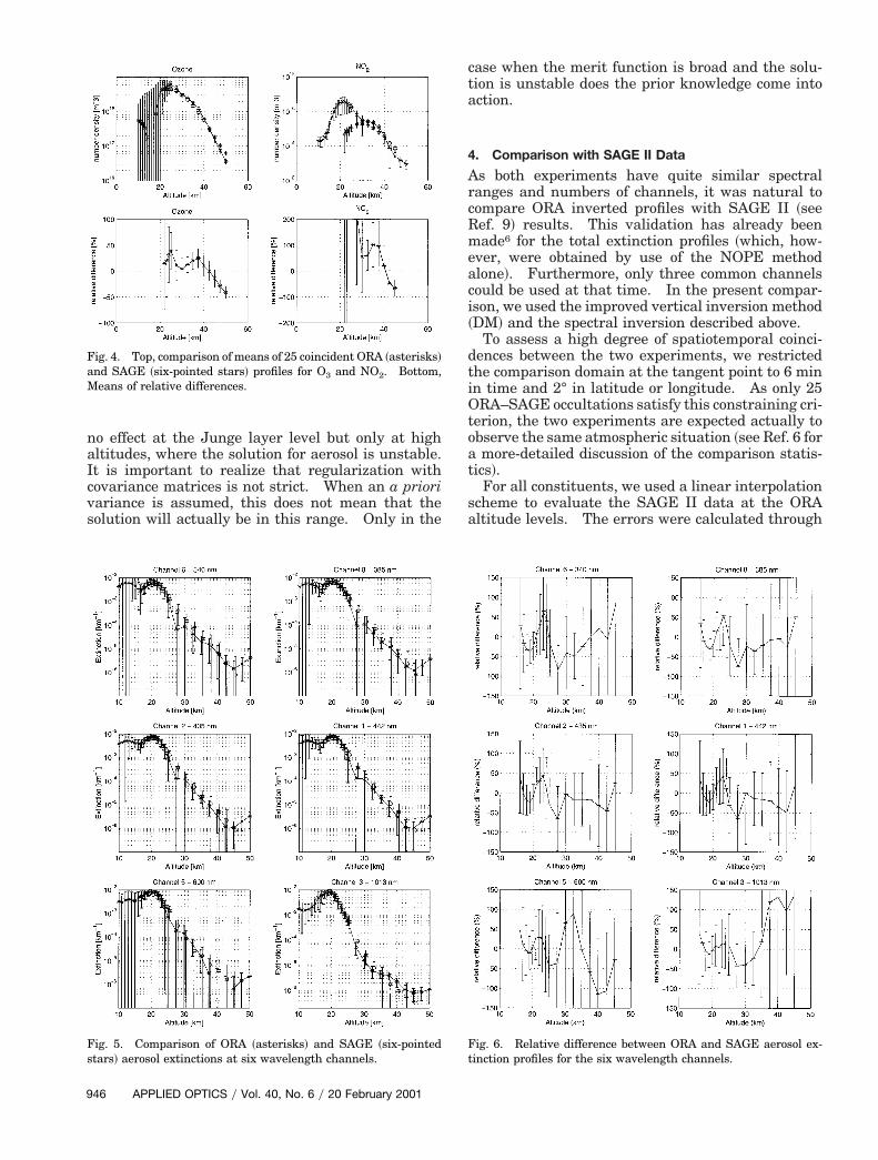
Fig. 4. Top, comparison of means of 25 coincident ORA ~asterisks!and SAGE ~six-pointed stars! profiles for O3 and NO2. Bottom,
eans of relative differences.
46 APPLIED OPTICS y Vol. 40, No. 6 y 20 February 2001
case when the merit function is broad and the solu-tion is unstable does the prior knowledge come intoaction.
4. Comparison with SAGE II Data
As both experiments have quite similar spectralranges and numbers of channels, it was natural tocompare ORA inverted profiles with SAGE II ~seeRef. 9! results. This validation has already beenmade6 for the total extinction profiles ~which, how-ever, were obtained by use of the NOPE methodalone!. Furthermore, only three common channelscould be used at that time. In the present compar-ison, we used the improved vertical inversion method~DM! and the spectral inversion described above.
To assess a high degree of spatiotemporal coinci-dences between the two experiments, we restrictedthe comparison domain at the tangent point to 6 minin time and 2° in latitude or longitude. As only 25ORA–SAGE occultations satisfy this constraining cri-terion, the two experiments are expected actually toobserve the same atmospheric situation ~see Ref. 6 fora more-detailed discussion of the comparison statis-tics!.
For all constituents, we used a linear interpolationscheme to evaluate the SAGE II data at the ORAaltitude levels. The errors were calculated through
Fig. 5. Comparison of ORA ~asterisks! and SAGE ~six-pointedstars! aerosol extinctions at six wavelength channels.
Fig. 6. Relative difference between ORA and SAGE aerosol ex-tinction profiles for the six wavelength channels.
S
mpda
solSiPmOu
ceutwmlaw
wwa
I
combination of the statistical variance of the 25 pro-files with the individual profile errors:
e2 5( ~pi 2 p# !2
n1
( ei2
n, (28)
where pi and ei are the ith profile and its error, re-spectively. The relative difference between the twoexperiments is evaluated as 100 3 ~ORA 2 SAGE!y
AGE.The results for O3 and NO2 are depicted in Fig. 4.
Data for SAGE II were available only in the altituderange from 20 to 50 km. For O3, the difference is atmost 40%. The NO2 profiles are also in fair agree-
ent, except at lower altitudes, where the ORA meanrofile is abnormally large. The main reason for thisisagreement is probably the coupling between theerosols and NO2 during the spectral inversion, be-
cause the spurious peak of the NO2 profile occurs atthe same altitude as the aerosol peak. Also, this isan altitude region where the relative contribution ofNO2 to the total extinction is very low compared withthose of other constituents.
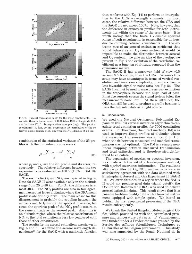
The results for the aerosol extinctions are shown inFig. 5 and 6. We fitted the aerosol wavelength de-pendence10 for the SAGE with a quadratic function
Fig. 7. Typical correlation plots for the three constituents. Re-sults for the occultation event of 10 October 1992 at longitude 13.5°and latitude 27.1°. Interpretation example ~top!: The point atcoordinates ~30 km, 20 km! represents the correlation of the re-trieved ozone density at 30 km with the NO2 density at 20 km.
that conforms with Eq. ~14! to perform an interpola-tion to the ORA wavelength channels. In mostcases, the relative difference between the ORA andthe SAGE did not exceed 100%. Note, however, thatthe difference in extinction profiles for both instru-ments fits within the range of the error bars. It isworth noting that the finite UV–visible spectralrange of both experiments is responsible for an irre-ducible coupling between constituents. In the ex-treme case of an aerosol extinction coefficient thatwould behave as an O3 cross section, it would beimpossible to make the distinction between aerosoland O3 content. To give an idea of the overlap, wepresent in Fig. 7 the evolution of the correlation co-efficient as a function of altitude, computed from thecovariance matrix.
The SAGE II has a narrower field of view ~0.5arcmin 3 2.5 arcmin! than the ORA. Whereas thisetup may have advantages in terms of vertical res-lution and inversion complexity, it suffers from aess favorable signal-to-noise ratio ~see Fig. 5!. TheAGE II cannot be used to measure aerosol extinction
n the troposphere because the huge load of post-inatubo aerosols causes the signal to drop below theeasurement noise level. At these altitudes, theRA can still be used to produce a profile because itses the full solar disk as a light source.
5. Conclusions
We used the Natural Orthogonal Polynomial Ex-pansion ~NOPE! vertical inversion algorithm to cal-ulate total extinction profiles for 7000 occultationvents. Furthermore, the direct method ~DM! wassed to improve these profiles at altitudes wherehe measured transmission was almost 0 or 1 orhen the fit between measured and modeled trans-ission was not optimal. The DM is a simple non-
inear mapping between measured transmissionnd total extinction and is therefore straightfor-ard to calculate.The separation of species, or spectral inversion,as made with the aid of a least-squares method,ith a priori covariance information. The resultantltitude profiles for O3, NO2, and aerosols were in
satisfactory agreement with the data obtained withStratospheric Aerosol and Gas Experiment II ~SAGEII!. At lower altitudes, in a region where the SAGEI could not produce good data ~signal cutoff !, the
Occultation Radiometer ~ORA! was used to deliveraerosol extinction data. This result shows that it ispossible to obtain quality data with a low-cost instru-ment equipped with simple optics. We intend topublish the first geophysical processing of the ORAresults subsequently.
We thank the United Kingdom Meteorological Of-fice, which provided us with the assimilated pres-sure and temperature data sets. F. Vanhellemontwas funded under a Prodex contract granted by theService des Affaires Scientifiques, Techniques etCulturelles of the Belgian government. This studywas also supported by the Fonds National de la
20 February 2001 y Vol. 40, No. 6 y APPLIED OPTICS 947
5. D. Fussen, E. Arijs, D. Nevejans, and F. Leclere, “Tomography
9
Recherche Scientifique of Belgium under grant1.5.155.98.
References1. E. Arijs, D. Nevejans, D. Fussen, P. Frederick, E. Van Rans-
beeck, F. W. Taylor, S. B. Calcutt, S. T. Werrett, C. L. Hepple-white, T. M. Pritchard, I. Burchell, and C. D. Rodgers, “TheORA ocultation radiometer on EURECA: instrument descrip-tion and preliminary results,” Adv. Space Res. 16, 33–36(1995).
2. W. P. Chu, M. P. McCormick, J. Lenoble, C. Brogniez, and P.Pruvost, “SAGE II inversion algorithm,” J. Geophys. Res. 94,8839–8351 ~1989!.
3. L. E. Mauldin III, N. H. Zaun, M. P. McCormick, J. H. Guy, andW. R. Vaughn, “Stratospheric Aerosol and Gas Experiment IIinstrument: a functional description,” Opt. Eng. 24, 307–312~1985!.
4. C. D. Rodgers, “Retrieval of atmospheric temperature and com-position from remote measurements of thermal radiation,”Rev. Geophys. Space Phys. 18, 609–624 ~1976!.
48 APPLIED OPTICS y Vol. 40, No. 6 y 20 February 2001
of the Earth’s atmosphere by the space-borne ORA radiometer:spatial inversion algorithm,” J. Geophys. Res. 102, 4357–4365~1997!.
6. D. Fussen, E. Arijs, D. Nevejans, F. V. Hellemont, C.Brogniez, and J. Lenoble, “Validation of the ORA spatialinversion algorithm with respect to the Stratospheric Aero-sol and Gas Experiment II data,” Appl. Opt. 37, 3121–3127~1998!.
7. C. D. Rodgers, “Characterization and error analysis of profilesretrieved from remote sounding measurements,” J. Geophys.Res. 95, 5587–5595 ~1990!.
8. A. Tarentola, Inverse Problem Theory ~Elsevier, Amsterdam,1987!.
9. J. Lenoble, “Presentation of the European correlative experi-ment program for SAGE II,” J. Geophys. Res. 94, 8395–8398~1989!.
10. C. Brogniez and J. Lenoble, “Analysis of 5-year aerosol datafrom the stratospheric aerosol and gas experiment,” J. Geo-phys. Res. 96, 15,479–15,497 ~1991!.