PoS(MCCT-SKADS)006 Front-end and Back-end in radioastronomy Enzo Natale * INAF Istituto di Radioastronomia E-mail: [email protected]Renzo Nesti Osservatorio Astrofisico di Arcetri E-mail: [email protected]In this paper we describe high performance microwave components commonly used in large band- width receivers for the centimetric and millimetric frequency range. Limitations to the ideal re- ceiver sensitivity due to different sources of noise are discussed. Finally two different focal plane arrays, which offer a major way to increase the data rate of astronomical observation of extended sources, are presented. First MCCT-SKADS Training School September 23-29, 2007 Medicina, Bologna Italy * Speaker. c Copyright owned by the author(s) under the terms of the Creative Commons Attribution-NonCommercial-ShareAlike Licence. http://pos.sissa.it/
Transcript
PoS(MCCT-SKADS)006
Front-end and Back-end in radioastronomy
Enzo Natale∗INAF Istituto di RadioastronomiaE-mail: [email protected]
Renzo NestiOsservatorio Astrofisico di ArcetriE-mail: [email protected]
In this paper we describe high performance microwave components commonly used in large band-width receivers for the centimetric and millimetric frequency range. Limitations to the ideal re-ceiver sensitivity due to different sources of noise are discussed. Finally two different focal planearrays, which offer a major way to increase the data rate of astronomical observation of extendedsources, are presented.
First MCCT-SKADS Training SchoolSeptember 23-29, 2007Medicina, Bologna Italy
Front-end and Back-end in radioastronomy Enzo Natale
1. Introduction
Purpose of these notes are to give some information on the technical aspects to be faced indesigning and building heterodyne receivers for radioastronomy. Of course not all aspects wouldbe covered in detail in the short time we have; certainly not in the few pages of this paper, sowe will focus our attention on arguments which seems to us of relevant importance. One mustalso consider the fact that the sensitivity of modern radioreceivers is approaching, at least in somebands, the quantum limit, so the only way to increase the time productivity of large antennas isto increase the "instantaneous" field of view or, in other words, the number of detectors. This canbe achieved with the deployment of focal plane arrays or phased arrays. Both these approacheswill require strong efforts in solving problems involved both in building complex receivers and inthe handling, storing and analyzing huge amount of data. Here we deal with single dish systemsapproach because of their flexibility and because they can be also used as elements of synthesisarrays like VLBI and similar networks.
2. The basic receiver
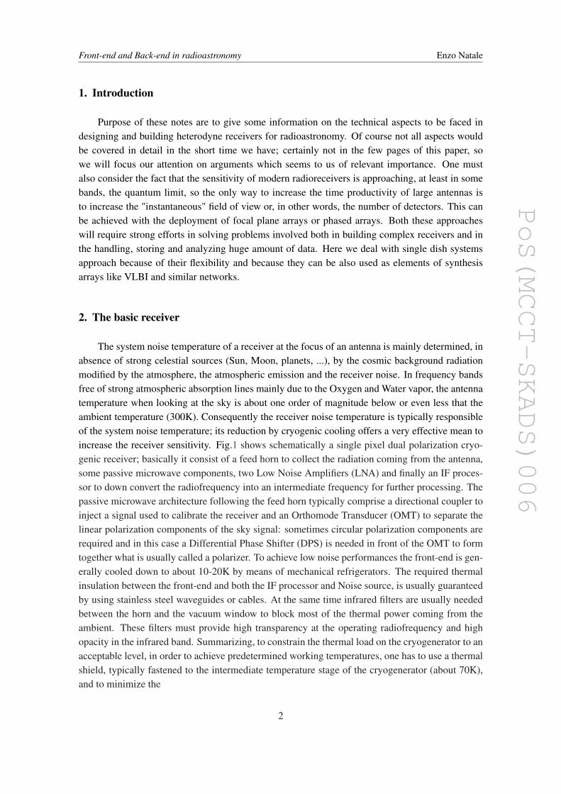
The system noise temperature of a receiver at the focus of an antenna is mainly determined, inabsence of strong celestial sources (Sun, Moon, planets, ...), by the cosmic background radiationmodified by the atmosphere, the atmospheric emission and the receiver noise. In frequency bandsfree of strong atmospheric absorption lines mainly due to the Oxygen and Water vapor, the antennatemperature when looking at the sky is about one order of magnitude below or even less that theambient temperature (300K). Consequently the receiver noise temperature is typically responsibleof the system noise temperature; its reduction by cryogenic cooling offers a very effective mean toincrease the receiver sensitivity. Fig.1 shows schematically a single pixel dual polarization cryo-genic receiver; basically it consist of a feed horn to collect the radiation coming from the antenna,some passive microwave components, two Low Noise Amplifiers (LNA) and finally an IF proces-sor to down convert the radiofrequency into an intermediate frequency for further processing. Thepassive microwave architecture following the feed horn typically comprise a directional coupler toinject a signal used to calibrate the receiver and an Orthomode Transducer (OMT) to separate thelinear polarization components of the sky signal: sometimes circular polarization components arerequired and in this case a Differential Phase Shifter (DPS) is needed in front of the OMT to formtogether what is usually called a polarizer. To achieve low noise performances the front-end is gen-erally cooled down to about 10-20K by means of mechanical refrigerators. The required thermalinsulation between the front-end and both the IF processor and Noise source, is usually guaranteedby using stainless steel waveguides or cables. At the same time infrared filters are usually neededbetween the horn and the vacuum window to block most of the thermal power coming from theambient. These filters must provide high transparency at the operating radiofrequency and highopacity in the infrared band. Summarizing, to constrain the thermal load on the cryogenerator to anacceptable level, in order to achieve predetermined working temperatures, one has to use a thermalshield, typically fastened to the intermediate temperature stage of the cryogenerator (about 70K),and to minimize the
2
PoS(MCCT-SKADS)006
Front-end and Back-end in radioastronomy Enzo Natale
Figure 1: Layout of a single beam, dual polarization, cryogenic receiver
• radiative power coming through the vacuum window by using suitable infrared blockingfilters;
• thermal exchanges between the dewar walls and the shield by using superinsulation [3];
• power due to the Joule effect and the thermal conductivity of the harness.
In the following a brief description of the basic components are given.
2.1 Feed horn
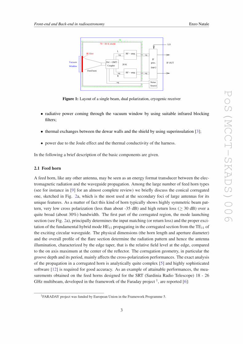
A feed horn, like any other antenna, may be seen as an energy format transducer between the elec-tromagnetic radiation and the waveguide propagation. Among the large number of feed horn types(see for instance in [9] for an almost complete review) we briefly discuss the conical corrugatedone, sketched in Fig. 2a, which is the most used at the secondary foci of large antennas for itsunique features. As a matter of fact this kind of horn typically shows highly symmetric beam pat-tern, very low cross polarization (less than about -35 dB) and high return loss (≥ 30 dB) over aquite broad (about 30%) bandwidth. The first part of the corrugated region, the mode launchingsection (see Fig. 2a), principally determines the input matching (or return loss) and the proper exci-tation of the fundamental hybrid mode HE11 propagating in the corrugated section from the TE11 ofthe exciting circular waveguide. The physical dimensions (the horn length and aperture diameter)and the overall profile of the flare section determine the radiation pattern and hence the antennaillumination, characterized by the edge taper, that is the relative field level at the edge, comparedto the on axis maximum at the center of the reflector. The corrugation geometry, in particular thegroove depth and its period, mainly affects the cross-polarization performances. The exact analysisof the propagation in a corrugated horn is analytically quite complex [5] and highly sophisticatedsoftware [12] is required for good accuracy. As an example of attainable performances, the mea-surements obtained on the feed horns designed for the SRT (Sardinia Radio Telescope) 18 - 26GHz multibeam, developed in the framework of the Faraday project 1, are reported [6]:
1FARADAY project was funded by European Union in the Framework Programme 5.
3
PoS(MCCT-SKADS)006
Front-end and Back-end in radioastronomy Enzo Natale
R
a
z
α waist
w0
a b
Figure 2: a) Cross section of a corrugated feed horn. b) Geometrical and Gaussian fundamental beam modeparameters
Return loss : ≥ 30 dBInsertion loss : ≤ -0.1 dBOff axis cross polarization : ≤ -30 dBBandwidth : 30% or larger
and illustrated in Fig. 3
To evaluate the performances achievable at the focus of a large antenna, i.e. an antenna whosediameter D is much larger than the wavelength λ , it is sufficient to give here some results based onthe approximation of the electromagnetic field distribution in terms of Gaussian beam modes (in[9] there is a very good and complete treatment of the argument).
In this approximation, it can be shown [9] that, for a not too large flare angle α and an apertureradius a greater than the wavelength (see Fig. 2b) a feed horn produces a gaussian beam whosewaist radius is w = 0.644 a located inside the horn at a distance z approximately equal to 1/3 ofthe horn length. In these conditions about 98% of the power radiated by the horn can be associatedwith the fundamental Gaussian beam mode. Using the standard formulae for Gaussian mode prop-agation [9], it becomes simple to compute the antenna illumination (the taper T ) and consequentlythe Full Width to Half Maximum beam width in the sky (FWHM) which, for a in-focus system andunblocked aperture, is given by:
4θFWHM = (1.02+0.0135T (dB))λ
Drad
2.2 DPS and OMT
To increase the capability and versatility of the antenna system, dual polarization operation isoften required. This can be done using a single feed (operating in dual polarization mode) withthe separation of the two orthogonal linearly polarized signals by using OMTs. Further, if it isdesired to separate the circular polarizations, a wide-band Differential Phase Shifter (DPS), whichtransforms circular to linear polarizations, can be inserted between the horn and the OMT. Theperformances generally required for astronomical observations to the combination DPS+OMT are:
4
PoS(MCCT-SKADS)006
Front-end and Back-end in radioastronomy Enzo Natale
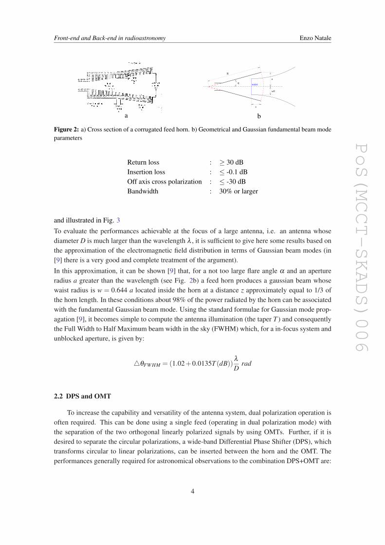
Figure 3: Copolar E-plane pattern of the feed horn for the 18-26 GHz multibeam
a b
Figure 4: a) Bøifot dual junction and b) Differential Phase shifter.
Return Loss : ≤ -20 dBInsertion Loss : ≤ 0.2 dBIsolationInput port - Output port : ≥ 40 dBbetween Output ports : ' 25 dBBandwidth : 30% or higher
There are various OMT designs (for a review see for instance [8]) commonly used operating withacceptable performance over a limited bandwidth, typically between 10% and 20%. Much widerbandwidths, of the order of 30% or higher, to match the bandwidth attainable by circular corrugatedhorns, can be obtained by using, for instance, the rectangular waveguide dual junctions as devel-oped by Bøifot [2] (depicted in Fig. 4a) or its derivation, see for instance [1] and the referencestherein cited , or the turnstile solution [14].
5
PoS(MCCT-SKADS)006
Front-end and Back-end in radioastronomy Enzo Natale
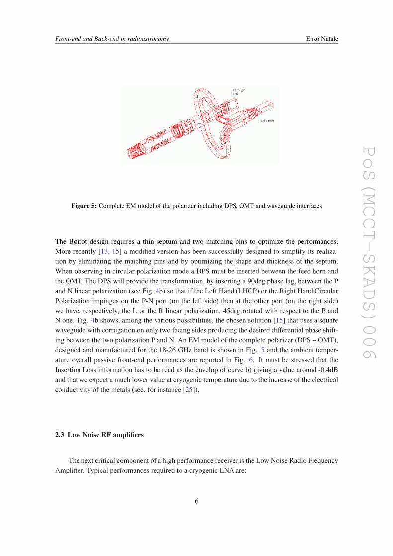
Figure 5: Complete EM model of the polarizer including DPS, OMT and waveguide interfaces
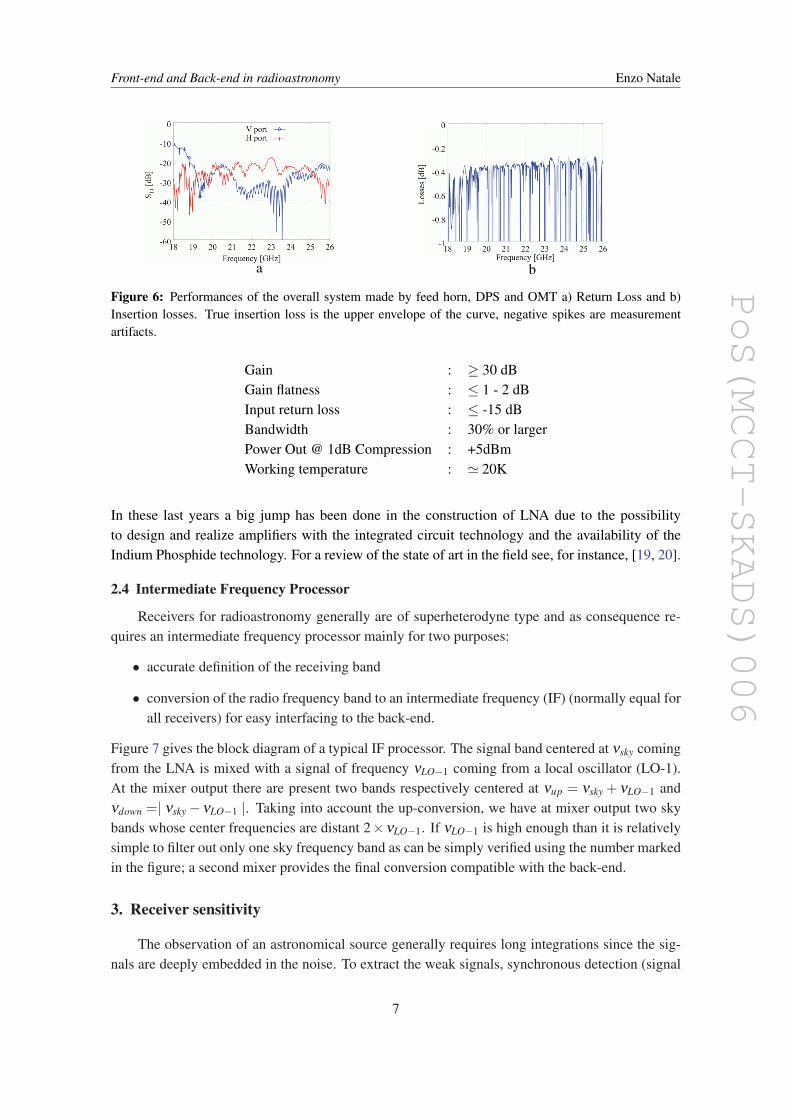
The Bøifot design requires a thin septum and two matching pins to optimize the performances.More recently [13, 15] a modified version has been successfully designed to simplify its realiza-tion by eliminating the matching pins and by optimizing the shape and thickness of the septum.When observing in circular polarization mode a DPS must be inserted between the feed horn andthe OMT. The DPS will provide the transformation, by inserting a 90deg phase lag, between the Pand N linear polarization (see Fig. 4b) so that if the Left Hand (LHCP) or the Right Hand CircularPolarization impinges on the P-N port (on the left side) then at the other port (on the right side)we have, respectively, the L or the R linear polarization, 45deg rotated with respect to the P andN one. Fig. 4b shows, among the various possibilities, the chosen solution [15] that uses a squarewaveguide with corrugation on only two facing sides producing the desired differential phase shift-ing between the two polarization P and N. An EM model of the complete polarizer (DPS + OMT),designed and manufactured for the 18-26 GHz band is shown in Fig. 5 and the ambient temper-ature overall passive front-end performances are reported in Fig. 6. It must be stressed that theInsertion Loss information has to be read as the envelop of curve b) giving a value around -0.4dBand that we expect a much lower value at cryogenic temperature due to the increase of the electricalconductivity of the metals (see. for instance [25]).
2.3 Low Noise RF amplifiers
The next critical component of a high performance receiver is the Low Noise Radio FrequencyAmplifier. Typical performances required to a cryogenic LNA are:
6
PoS(MCCT-SKADS)006
Front-end and Back-end in radioastronomy Enzo Natale
a b
Figure 6: Performances of the overall system made by feed horn, DPS and OMT a) Return Loss and b)Insertion losses. True insertion loss is the upper envelope of the curve, negative spikes are measurementartifacts.
Gain : ≥ 30 dBGain flatness : ≤ 1 - 2 dBInput return loss : ≤ -15 dBBandwidth : 30% or largerPower Out @ 1dB Compression : +5dBmWorking temperature : ' 20K
In these last years a big jump has been done in the construction of LNA due to the possibilityto design and realize amplifiers with the integrated circuit technology and the availability of theIndium Phosphide technology. For a review of the state of art in the field see, for instance, [19, 20].
2.4 Intermediate Frequency Processor
Receivers for radioastronomy generally are of superheterodyne type and as consequence re-quires an intermediate frequency processor mainly for two purposes:
• accurate definition of the receiving band
• conversion of the radio frequency band to an intermediate frequency (IF) (normally equal forall receivers) for easy interfacing to the back-end.
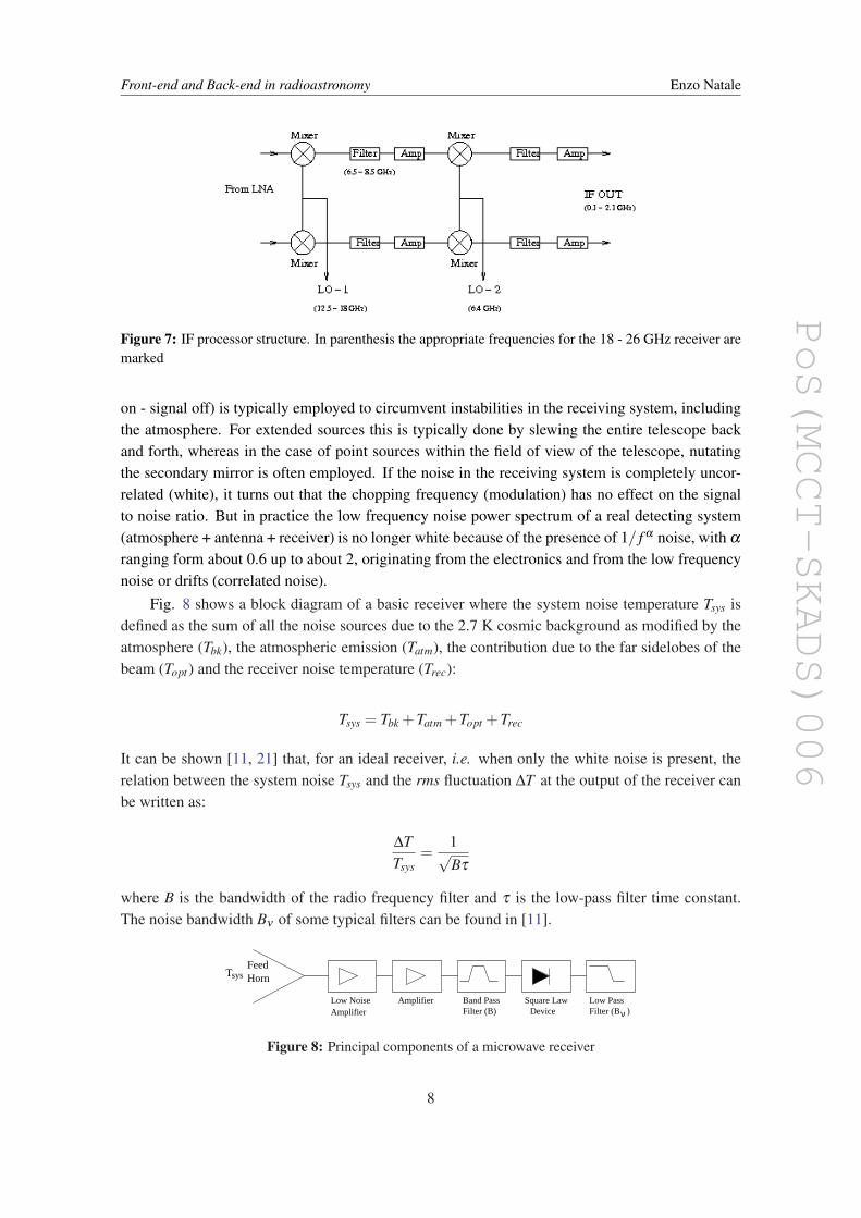
Figure 7 gives the block diagram of a typical IF processor. The signal band centered at νsky comingfrom the LNA is mixed with a signal of frequency νLO−1 coming from a local oscillator (LO-1).At the mixer output there are present two bands respectively centered at νup = νsky + νLO−1 andνdown =| νsky−νLO−1 |. Taking into account the up-conversion, we have at mixer output two skybands whose center frequencies are distant 2×νLO−1. If νLO−1 is high enough than it is relativelysimple to filter out only one sky frequency band as can be simply verified using the number markedin the figure; a second mixer provides the final conversion compatible with the back-end.
3. Receiver sensitivity
The observation of an astronomical source generally requires long integrations since the sig-nals are deeply embedded in the noise. To extract the weak signals, synchronous detection (signal
7
PoS(MCCT-SKADS)006
Front-end and Back-end in radioastronomy Enzo Natale
Figure 7: IF processor structure. In parenthesis the appropriate frequencies for the 18 - 26 GHz receiver aremarked
on - signal off) is typically employed to circumvent instabilities in the receiving system, includingthe atmosphere. For extended sources this is typically done by slewing the entire telescope backand forth, whereas in the case of point sources within the field of view of the telescope, nutatingthe secondary mirror is often employed. If the noise in the receiving system is completely uncor-related (white), it turns out that the chopping frequency (modulation) has no effect on the signalto noise ratio. But in practice the low frequency noise power spectrum of a real detecting system(atmosphere + antenna + receiver) is no longer white because of the presence of 1/ f α noise, with α
ranging form about 0.6 up to about 2, originating from the electronics and from the low frequencynoise or drifts (correlated noise).
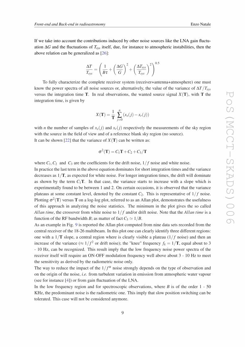
Fig. 8 shows a block diagram of a basic receiver where the system noise temperature Tsys isdefined as the sum of all the noise sources due to the 2.7 K cosmic background as modified by theatmosphere (Tbk), the atmospheric emission (Tatm), the contribution due to the far sidelobes of thebeam (Topt) and the receiver noise temperature (Trec):
Tsys = Tbk +Tatm +Topt +Trec
It can be shown [11, 21] that, for an ideal receiver, i.e. when only the white noise is present, therelation between the system noise Tsys and the rms fluctuation ∆T at the output of the receiver canbe written as:
∆TTsys
=1√Bτ
where B is the bandwidth of the radio frequency filter and τ is the low-pass filter time constant.The noise bandwidth Bν of some typical filters can be found in [11].
sysFeedHorn
AmplifierLow NoiseAmplifier
Band PassFilter (B)
Square LawDevice
Low Pass
ν )Filter (B
T
Figure 8: Principal components of a microwave receiver
8
PoS(MCCT-SKADS)006
Front-end and Back-end in radioastronomy Enzo Natale
If we take into account the contributions induced by other noise sources like the LNA gain fluctu-ation ∆G and the fluctuations of Tsys itself, due, for instance to atmospheric instabilities, then theabove relation can be generalized as [26]:
∆TTsys
=
(1
Bτ+(
∆GG
)2
+(
∆Tsys
Tsys
)2)0.5
To fully characterize the complete receiver system (receiver+antenna+atmosphere) one mustknow the power spectra of all noise sources or, alternatively, the value of the variance of ∆T/Tsys
versus the integration time T. In real observations, the wanted source signal X(T), with T theintegration time, is given by
X(T) =1T
n
∑j=0
(xs( j)− xr( j))
with n the number of samples of xs( j) and xr( j) respectively the measurements of the sky regionwith the source in the field of view and of a reference blank sky region (no source).It can be shown [22] that the variance of X(T) can be written as:
σ2(T) = C1T+C2 +C3/T
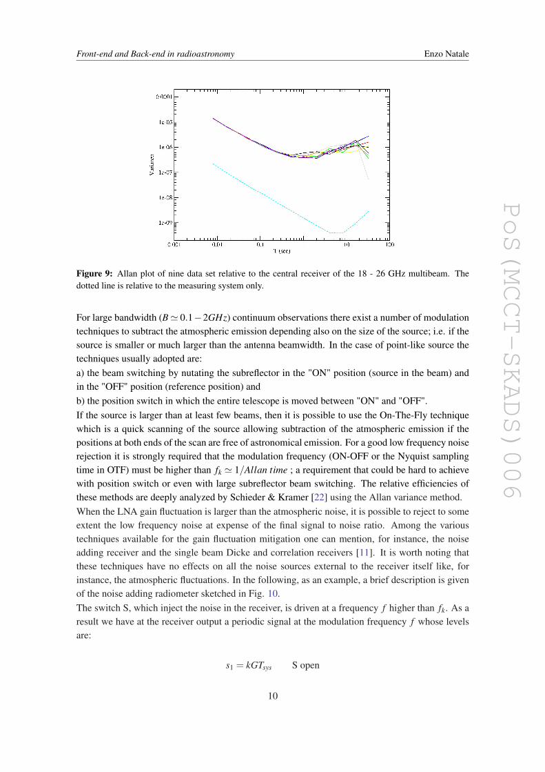
where C1,C2 and C3 are the coefficients for the drift noise, 1/ f noise and white noise.In practice the last term in the above equation dominates for short integration times and the variancedecreases as 1/T, as expected for white noise. For longer integration times, the drift will dominateas shown by the term C1T. In that case, the variance starts to increase with a slope which isexperimentally found to be between 1 and 2. On certain occasions, it is observed that the varianceplateaus at some constant level, denoted by the constant C2. This is representative of 1/ f noise.Plotting σ2(T) versus T on a log-log plot, referred to as an Allan plot, demonstrates the usefulnessof this approach in analyzing the noise statistics. The minimum in the plot gives the so calledAllan time, the crossover from white noise to 1/ f and/or drift noise. Note that the Allan time is afunction of the RF bandwidth B; as matter of fact C3 ' 1/B.As an example in Fig. 9 is reported the Allan plot computed from nine data sets recorded from thecentral receiver of the 18-26 multibeam. In this plot one can clearly identify three different regions:one with a 1/T slope, a central region where is clearly visible a plateau (1/ f noise) and then anincrease of the variance (≈ 1/ f 2 or drift noise); the "knee" frequency fk = 1/T, equal about to 3- 10 Hz, can be recognized. This result imply that the low frequency noise power spectra of thereceiver itself will require an ON-OFF modulation frequency well above about 3 - 10 Hz to meetthe sensitivity as derived by the radiometric noise only.The way to reduce the impact of the 1/ f α noise strongly depends on the type of observation andon the origin of the noise, i.e. from turbulent variation in emission from atmospheric water vapour(see for instance [4]) or from gain fluctuation of the LNA.In the low frequency region and for spectroscopic observations, where B is of the order 1 - 50KHz, the predominant noise is the radiometric one. This imply that slow position switching can betolerated. This case will not be considered anymore.
9
PoS(MCCT-SKADS)006
Front-end and Back-end in radioastronomy Enzo Natale
Figure 9: Allan plot of nine data set relative to the central receiver of the 18 - 26 GHz multibeam. Thedotted line is relative to the measuring system only.
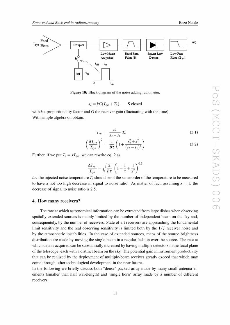
For large bandwidth (B' 0.1−2GHz) continuum observations there exist a number of modulationtechniques to subtract the atmospheric emission depending also on the size of the source; i.e. if thesource is smaller or much larger than the antenna beamwidth. In the case of point-like source thetechniques usually adopted are:a) the beam switching by nutating the subreflector in the "ON" position (source in the beam) andin the "OFF" position (reference position) andb) the position switch in which the entire telescope is moved between "ON" and "OFF".If the source is larger than at least few beams, then it is possible to use the On-The-Fly techniquewhich is a quick scanning of the source allowing subtraction of the atmospheric emission if thepositions at both ends of the scan are free of astronomical emission. For a good low frequency noiserejection it is strongly required that the modulation frequency (ON-OFF or the Nyquist samplingtime in OTF) must be higher than fk ' 1/Allan time ; a requirement that could be hard to achievewith position switch or even with large subreflector beam switching. The relative efficiencies ofthese methods are deeply analyzed by Schieder & Kramer [22] using the Allan variance method.When the LNA gain fluctuation is larger than the atmospheric noise, it is possible to reject to someextent the low frequency noise at expense of the final signal to noise ratio. Among the varioustechniques available for the gain fluctuation mitigation one can mention, for instance, the noiseadding receiver and the single beam Dicke and correlation receivers [11]. It is worth noting thatthese techniques have no effects on all the noise sources external to the receiver itself like, forinstance, the atmospheric fluctuations. In the following, as an example, a brief description is givenof the noise adding radiometer sketched in Fig. 10.The switch S, which inject the noise in the receiver, is driven at a frequency f higher than fk. As aresult we have at the receiver output a periodic signal at the modulation frequency f whose levelsare:
s1 = kGTsys S open
10
PoS(MCCT-SKADS)006
Front-end and Back-end in radioastronomy Enzo Natale
Figure 10: Block diagram of the noise adding radiometer.
s2 = kG(Tsys +Tn) S closed
with k a proportionality factor and G the receiver gain (fluctuating with the time).With simple algebra on obtain:
Tsys =s1
s2− s1Tn (3.1)(
∆Tsys
Tsys
)2
=1
Bτ
(1+
s22 + s2
1(s2− s1)2
)(3.2)
Further, if we put Tn = xTsys, we can rewrite eq. 2 as
∆Tsys
Tsys=
√2
Bτ
(1+
1x
+1x2
)0.5
i.e. the injected noise temperature Tn should be of the same order of the temperature to be measuredto have a not too high decrease in signal to noise ratio. As matter of fact, assuming x = 1, thedecrease of signal to noise ratio is 2.5.
4. How many receivers?
The rate at which astronomical information can be extracted from large dishes when observingspatially extended sources is mainly limited by the number of independent beam on the sky and,consequentely, by the number of receivers. State of art receivers are approaching the fundamentallimit sensitivity and the real observing sensitivity is limited both by the 1/ f receiver noise andby the atmospheric instabilities. In the case of extended sources, maps of the source brightnessdistribution are made by moving the single beam in a regular fashion over the source. The rate atwhich data is acquired can be substantially increased by having multiple detectors in the focal planeof the telescope, each with a distinct beam on the sky. The potential gain in instrument productivitythat can be realized by the deployment of multiple-beam receiver greatly exceed that which maycome through other technological development in the near future.In the following we briefly discuss both "dense" packed array made by many small antenna el-ements (smaller than half wavelength) and "single horn" array made by a number of differentreceivers.
11
PoS(MCCT-SKADS)006
Front-end and Back-end in radioastronomy Enzo Natale
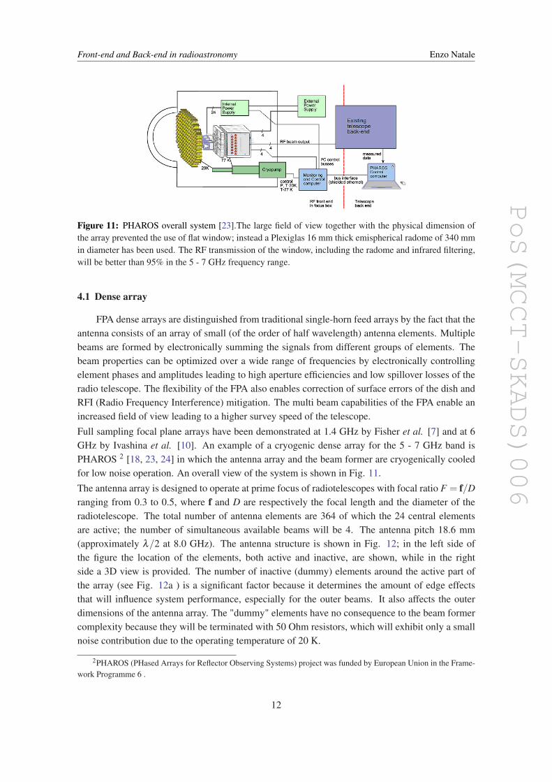
Figure 11: PHAROS overall system [23].The large field of view together with the physical dimension ofthe array prevented the use of flat window; instead a Plexiglas 16 mm thick emispherical radome of 340 mmin diameter has been used. The RF transmission of the window, including the radome and infrared filtering,will be better than 95% in the 5 - 7 GHz frequency range.
4.1 Dense array
FPA dense arrays are distinguished from traditional single-horn feed arrays by the fact that theantenna consists of an array of small (of the order of half wavelength) antenna elements. Multiplebeams are formed by electronically summing the signals from different groups of elements. Thebeam properties can be optimized over a wide range of frequencies by electronically controllingelement phases and amplitudes leading to high aperture efficiencies and low spillover losses of theradio telescope. The flexibility of the FPA also enables correction of surface errors of the dish andRFI (Radio Frequency Interference) mitigation. The multi beam capabilities of the FPA enable anincreased field of view leading to a higher survey speed of the telescope.Full sampling focal plane arrays have been demonstrated at 1.4 GHz by Fisher et al. [7] and at 6GHz by Ivashina et al. [10]. An example of a cryogenic dense array for the 5 - 7 GHz band isPHAROS 2 [18, 23, 24] in which the antenna array and the beam former are cryogenically cooledfor low noise operation. An overall view of the system is shown in Fig. 11.The antenna array is designed to operate at prime focus of radiotelescopes with focal ratio F = f/Dranging from 0.3 to 0.5, where f and D are respectively the focal length and the diameter of theradiotelescope. The total number of antenna elements are 364 of which the 24 central elementsare active; the number of simultaneous available beams will be 4. The antenna pitch 18.6 mm(approximately λ/2 at 8.0 GHz). The antenna structure is shown in Fig. 12; in the left side ofthe figure the location of the elements, both active and inactive, are shown, while in the rightside a 3D view is provided. The number of inactive (dummy) elements around the active part ofthe array (see Fig. 12a ) is a significant factor because it determines the amount of edge effectsthat will influence system performance, especially for the outer beams. It also affects the outerdimensions of the antenna array. The "dummy" elements have no consequence to the beam formercomplexity because they will be terminated with 50 Ohm resistors, which will exhibit only a smallnoise contribution due to the operating temperature of 20 K.
2PHAROS (PHased Arrays for Reflector Observing Systems) project was funded by European Union in the Frame-work Programme 6 .
12
PoS(MCCT-SKADS)006
Front-end and Back-end in radioastronomy Enzo Natale
a b
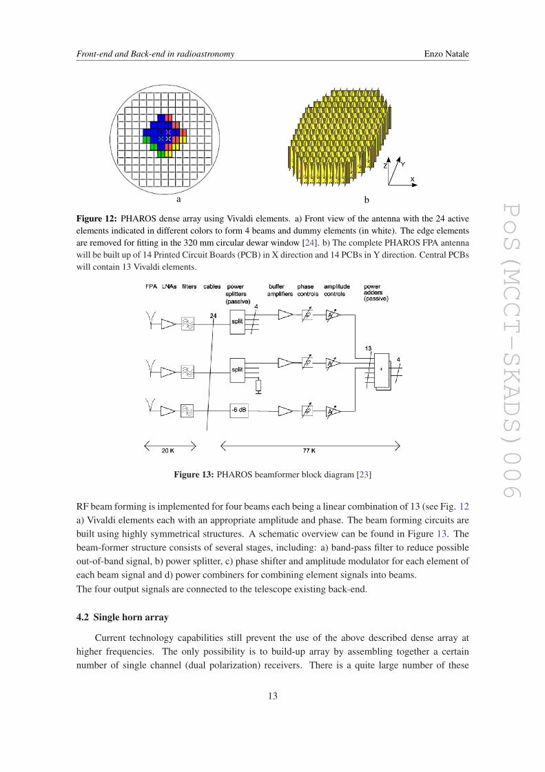
Figure 12: PHAROS dense array using Vivaldi elements. a) Front view of the antenna with the 24 activeelements indicated in different colors to form 4 beams and dummy elements (in white). The edge elementsare removed for fitting in the 320 mm circular dewar window [24]. b) The complete PHAROS FPA antennawill be built up of 14 Printed Circuit Boards (PCB) in X direction and 14 PCBs in Y direction. Central PCBswill contain 13 Vivaldi elements.
Figure 13: PHAROS beamformer block diagram [23]
RF beam forming is implemented for four beams each being a linear combination of 13 (see Fig. 12a) Vivaldi elements each with an appropriate amplitude and phase. The beam forming circuits arebuilt using highly symmetrical structures. A schematic overview can be found in Figure 13. Thebeam-former structure consists of several stages, including: a) band-pass filter to reduce possibleout-of-band signal, b) power splitter, c) phase shifter and amplitude modulator for each element ofeach beam signal and d) power combiners for combining element signals into beams.The four output signals are connected to the telescope existing back-end.
4.2 Single horn array
Current technology capabilities still prevent the use of the above described dense array athigher frequencies. The only possibility is to build-up array by assembling together a certainnumber of single channel (dual polarization) receivers. There is a quite large number of these
13
PoS(MCCT-SKADS)006
Front-end and Back-end in radioastronomy Enzo Natale
a b
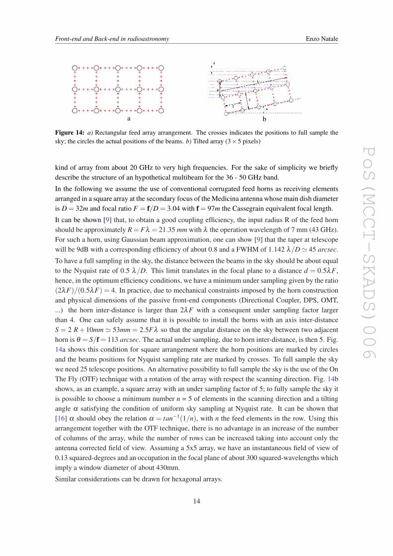
Figure 14: a) Rectangular feed array arrangement. The crosses indicates the positions to full sample thesky; the circles the actual positions of the beams. b) Tilted array (3×5 pixels)
kind of array from about 20 GHz to very high frequencies. For the sake of simplicity we brieflydescribe the structure of an hypothetical multibeam for the 36 - 50 GHz band.
In the following we assume the use of conventional corrugated feed horns as receiving elementsarranged in a square array at the secondary focus of the Medicina antenna whose main dish diameteris D = 32m and focal ratio F = f/D = 3.04 with f = 97m the Cassegrain equivalent focal length.
It can be shown [9] that, to obtain a good coupling efficiency, the input radius R of the feed hornshould be approximately R = Fλ = 21.35 mm with λ the operation wavelength of 7 mm (43 GHz).For such a horn, using Gaussian beam approximation, one can show [9] that the taper at telescopewill be 9dB with a corresponding efficiency of about 0.8 and a FWHM of 1.142 λ/D' 45 arcsec.
To have a full sampling in the sky, the distance between the beams in the sky should be about equalto the Nyquist rate of 0.5 λ/D. This limit translates in the focal plane to a distance d = 0.5λF ,hence, in the optimum efficiency conditions, we have a minimum under sampling given by the ratio(2λF)/(0.5λF) = 4. In practice, due to mechanical constraints imposed by the horn constructionand physical dimensions of the passive front-end components (Directional Coupler, DPS, OMT,...) the horn inter-distance is larger than 2λF with a consequent under sampling factor largerthan 4. One can safely assume that it is possible to install the horns with an axis inter-distanceS = 2 R + 10mm ' 53mm = 2.5Fλ so that the angular distance on the sky between two adjacenthorn is θ = S/f = 113 arcsec. The actual under sampling, due to horn inter-distance, is then 5. Fig.14a shows this condition for square arrangement where the horn positions are marked by circlesand the beams positions for Nyquist sampling rate are marked by crosses. To full sample the skywe need 25 telescope positions. An alternative possibility to full sample the sky is the use of the OnThe Fly (OTF) technique with a rotation of the array with respect the scanning direction. Fig. 14bshows, as an example, a square array with an under sampling factor of 5; to fully sample the sky itis possible to choose a minimum number n = 5 of elements in the scanning direction and a tiltingangle α satisfying the condition of uniform sky sampling at Nyquist rate. It can be shown that[16] α should obey the relation α = tan−1(1/n), with n the feed elements in the row. Using thisarrangement together with the OTF technique, there is no advantage in an increase of the numberof columns of the array, while the number of rows can be increased taking into account only theantenna corrected field of view. Assuming a 5x5 array, we have an instantaneous field of view of0.13 squared-degrees and an occupation in the focal plane of about 300 squared-wavelengths whichimply a window diameter of about 430mm.
Similar considerations can be drawn for hexagonal arrays.
14
PoS(MCCT-SKADS)006
Front-end and Back-end in radioastronomy Enzo Natale
5. Conclusions
To increase the observing efficiency one has to to recover a significant fraction of the infor-mation available in the focal plane of large radio telescopes; as a consequence, large arrays, of theorder of several tens of receivers, are needed in the millimetric bands. The near future efforts must,hence, be directed towards the making of high performance complete receivers far less expensiveand time consuming to construct and test.
ACKNOWLEDGMENTS The authors gratefully acknowlwdges many stimulating discus-sions with A. Orfei and G. Comoretto.
References
[1] R. Banham ,G. Valsecchi, L. Lucci, G. Pelosi, S. Selleri, V. Natale, R. Nesti and G. Tofani, G.,Electroformed Front-end at 100 GHz for Radioastronomical Applications, Microwave Journal 48, n.8,112, August 2005
[2] A.M. Bøifot, E. Lier and T. Shaug-Petersen, Simple and Broadband Orthomode Transducer, Proc.IEE, part H, Vol.137, n. 6, pp. 396-400, Dec. 1990.
[3] R.R. Conte, Elements de Cryogenie, Masson&Cie Editeurs, Paris, 1970
[4] S. Church, M.N.R.A.S., 272, 551, 1995
[5] P.J.B. Clarricoats and A.D. Olver, Corrugated Horn for Microwave Antennas, Peter Peregrinus,London, 1984
[6] Faraday - IRA Final Report, 2007
[7] J.R. Fisher and R.F. Bradley, R.F., Full-Sampling Focal Plane Arrays in Imaging at Radio throughSubmillimeter Wavelengths, ASP Conference Series, Vol. 217, J.G. Mangum and S.J.E. RadfordEditors, 2000
[8] G.G. Gentili, R. Nesti, G. Pelosi and S. Selleri, Orthomode Transducers in The Wiley Encyclopediaof RF and Microwave Engineering, John Wiley & Sons, (New York, NY, USA), Vol. 4, 2005
[9] P.F. Goldsmith, Quasioptical Systems: Gaussian Beam Quasioptical Propagation and Applications,IEEE Press, Piscataway, 1998
[10] M.V. Ivashina, J. Simons, and J.G. Bij de Vaate, Efficiency Analysis of Focal Plane Arrays in DeepDishes, Experimental Astronomy 17, pp.149-162, 2004.
[11] J.D. Kraus, Radio Astronomy, McGraw-Hill Book Company, 1966
[12] L. Lucci, R. Nesti, G. Pelosi, and S. Selleri, Corrugated Horns in The Wiley Enciclopedia of RF andMicrowave Engineering, John Wiley & Sons, (New York, NY, USA), Vol. 4, 2005
[13] G. Narayanan, and N.R. Erickson, Design and performance of a novel full-waveguide bandorthomode transducer, 13th Symposium On Space THz Technology, Cambridge,MA, 2002
[14] A. Navarrini and R.L. Plambeck, A Turnstile Junction Waveguide Orthomode Transducer, IEEE MTT54, n. 1, Jan 2006
[15] Nesti, R. et. al. The 22 GHz Polarizer Technical Report FARFI1 02/04, 2004
15
PoS(MCCT-SKADS)006
Front-end and Back-end in radioastronomy Enzo Natale
[16] A. Orfei, et al. Feasibility study for a multifeed in the 43GHz band, IRA Internal Report n. 401, 2007
[17] R. Padman, Optical Fundamentals for Array Feeds in Multi-Feed Systems for Radio Telescopes ASPConference Series, Volume 75, D.T. Emerson and J.M. Payne Editors, 1995
[18] PHAROS project (http://www.pharos-eu.org)
[19] M.W. Pospieszalski, Extremely Low-Noise Amplification with Cryogenic FETs and HFETs:1970-2004, NRAO ELECTRONICS DIVISION Internal Report NO. 314, 2005
[20] M.W. Pospieszalski, and E.J. Wollack, Characteristics of broadband InP HFET millimeter waveamplifiers and their applications in radioastronomy receivers, in Proc. of ESA Workshop onmm-wave, Helsinki, May 1998
[21] Rohlfs, K., Wilson, T.L., Tools of Radio Astronomy, Springer, 1996
[22] R. Schieder, and C. Kramer, Optimization of heterodyne observations, A&A 373, 746, 2001
[23] J. Simons, J.G. Bij de Vaate, M.V. Ivashina, M. Zuliani, V. Natale, and N. Roddis, Design of a focalplane array system at cryogenic temperatures, The European Conference on Antennas andPropagation: EuCAP 2006, ESA SP-626, Nice, 6 - 10 November 2006
[24] J. Simons, PHAROS System specifications Ver.0.7, June 2006
[26] E.J. Wollack, High-electron-mobility-transistor gain stability and its design implications for wideband millimeter wave receivers, Rev. Sci. Instrum. 66, August 1995, 4305