HAL Id: hal-00866058 https://hal.inria.fr/hal-00866058 Submitted on 25 Sep 2013 HAL is a multi-disciplinary open access archive for the deposit and dissemination of sci- entific research documents, whether they are pub- lished or not. The documents may come from teaching and research institutions in France or abroad, or from public or private research centers. L’archive ouverte pluridisciplinaire HAL, est destinée au dépôt et à la diffusion de documents scientifiques de niveau recherche, publiés ou non, émanant des établissements d’enseignement et de recherche français ou étrangers, des laboratoires publics ou privés. Repair Time in Distributed Storage Systems Frédéric Giroire, Sandeep Kumar Gupta, Remigiusz Modrzejewski, Julian Monteiro, Stéphane Perennes To cite this version: Frédéric Giroire, Sandeep Kumar Gupta, Remigiusz Modrzejewski, Julian Monteiro, Stéphane Perennes. Repair Time in Distributed Storage Systems. 6th International Conference on Data Man- agement in Cloud, Grid and P2P Systems (Globe 2013), Aug 2013, Prague, Czech Republic. pp.99-110, 10.1007/978-3-642-40053-7_9. hal-00866058
Transcript
HAL Id: hal-00866058https://hal.inria.fr/hal-00866058
Submitted on 25 Sep 2013
HAL is a multi-disciplinary open accessarchive for the deposit and dissemination of sci-entific research documents, whether they are pub-lished or not. The documents may come fromteaching and research institutions in France orabroad, or from public or private research centers.
L’archive ouverte pluridisciplinaire HAL, estdestinée au dépôt et à la diffusion de documentsscientifiques de niveau recherche, publiés ou non,émanant des établissements d’enseignement et derecherche français ou étrangers, des laboratoirespublics ou privés.
Repair Time in Distributed Storage SystemsFrédéric Giroire, Sandeep Kumar Gupta, Remigiusz Modrzejewski, Julian
Monteiro, Stéphane Perennes
To cite this version:Frédéric Giroire, Sandeep Kumar Gupta, Remigiusz Modrzejewski, Julian Monteiro, StéphanePerennes. Repair Time in Distributed Storage Systems. 6th International Conference on Data Man-agement in Cloud, Grid and P2P Systems (Globe 2013), Aug 2013, Prague, Czech Republic. pp.99-110,�10.1007/978-3-642-40053-7_9�. �hal-00866058�
Frederic Giroire1, Sandeep K. Gupta2, Remigiusz Modrzejewski1, JulianMonteiro3 and Stephane Perennes1
1Project MASCOTTE, I3S (CNRS/Univ. of Nice)/INRIA, Sophia Antipolis, France2IIT Delhi, New Delhi, India
3Department of Computer Science, IME, University of Sao Paulo, Brazil
Abstract. In this paper, we analyze a highly distributed backup stor-age system realized by means of nano datacenters (NaDa). NaDa havebeen recently proposed as a way to mitigate the growing energy, band-width and device costs of traditional data centers, following the popu-larity of cloud computing. These service provider-controlled peer-to-peersystems take advantage of resources already committed to always-on settop boxes, the fact they do not generate heat dissipation costs and theirproximity to users.
In this kind of systems redundancy is introduced to preserve the data incase of peer failures or departures. To ensure long-term fault tolerance,the storage system must have a self-repairing service that continuouslyreconstructs the fragments of redundancy that are lost. The speed ofthis reconstruction process is crucial for the data survival. This speedis mainly determined by how much bandwidth, which is a critical re-source of such systems, is available. In the literature, the reconstruc-tion times are modeled as independent (e.g., poissonian, deterministic,or more generally following any distribution). In practice, however, nu-merous reconstructions start at the same time (when the system detectsthat a peer has failed). Consequently, they are correlated to each otherbecause concurrent reconstructions do compete for the same bandwidth.This correlation negatively impacts the efficiency of the bandwidth uti-lization and henceforth the repair time.
We propose a new analytical framework that takes into account thiscorrelation when estimating the repair time and the probability of dataloss. Mainly, we introduce a queuing model in which reconstructions areserved by peers at a rate that depends on the available bandwidth. Weshow that the load is unbalanced among peers (young peers inherentlystore less data than the old ones). This leads us to introduce a correctingfactor on the repair rate of the system. The models and schemes proposedare validated by mathematical analysis, extensive set of simulations, andexperimentation using the GRID5000 test-bed platform. This new modelallows system designers to operate a more accurate choice of systemparameters in function of their targeted data durability.
? The research leading to these results has received funding from the European ProjectFP7 EULER, ANR CEDRE, ANR AGAPE, Associated Team AlDyNet, projectECOS-Sud Chile and region PACA.
2 Authors Suppressed Due to Excessive Length
1 Introduction
Nano datacenters (NaDa) are highly distributed systems owned and controlledby the service provider. This alleviates the need of incentives and mitigates therisk of malicious users, but otherwise they face the same challenges as peer-to-peer systems. The set-top boxes realizing them are connected using consumerlinks, which can be relatively slow, unreliable and congested. The devices them-selves, compared to servers in a traditional datacenter, are prone to failures andtemporary disconnections, e.g. if the user cuts the power supply when not inhome. When originally proposed in [1], they were assumed to be available nomore than 85% of the time, with values as low as 7% possible.
In this paper we concentrate on application of NaDa, or any similar peer-to-peer system, for backup storage. In this application, users want to store massiveamounts of data indefinitely, accessing them very rarely, i.e. only when originalcopies are lost. Due to risk of peer failures or departures, redundancy data isintroduced to ensure long term data survival. To this end, most of the proposedstorage systems use either the simple replication or the space efficient erasurecodes [2], such as the Reed-Solomon or Regenerating Codes [3]. The redundancyneeds to be maintained by a self-repair process. Its speed is crucial to determinethe system reliability, as long repairs exponentially increase the probability oflosing data. The limiting factor, in this setting, is the upload link capacity.
Imagine a scenario where the system is realized using home connections, outof which an average 128kbps are allocated to the backup application. Further-more, each device is limited to 300GB, while average data stored is 100GB,redundancy is double, 100 devices take part in each repair and the algorithmsare as described in the following sections. A naive back-of-envelope computa-tion gives that the time needed to repair contents of a failed device is 17 hours(= 100 · 8 · 106kb/(100 · 128kbps)). This translates, by our model, to a probabil-ity of data loss per year (PDLPY) of 10−8. But, taking into account all findingspresented in this work, the actual time can reach 9 days. This gives a PDLPYof 0.2, many orders of magnitude more than the naive computation. Hence, it isimportant to have models that estimate accurately the repair time for limitedbandwidth.
Our contribution
We propose a new analytical model that precisely estimates the repair timeand the probability of losing data in distributed storage systems. This modeltakes into account the bandwidth constraints and inherent workload imbalance(young peers inherently store less data than the old ones, thus they contributeasymmetrically to the reconstruction process) effect on the efficiency. It allowssystem designers to obtain an accurate choice of system parameters to obtain adesired data durability.
We discuss how far the distribution of the reconstruction time given by themodel is from the exponential, classically used in the literature. We exhibit thedifferent possible shapes of this distribution in function of the system parameters.
Repair Time in Distributed Storage Systems 3
This distribution impacts the durability of the system. We also show a somewhatcounter-intuitive result that we can reduce the reconstruction time by using aless bandwidth efficient Regenerating Code. This is due to a degree of freedomgiven by erasure codes to choose which peers participate in the repair process.
To the best of our knowledge, this is the first detailed model proposed toestimate the distribution of the reconstruction time under limited bandwidthconstraints. We validate our model by an extensive set of simulations and by test-bed experimentation using the Grid’5000 platform, see [4] for its description.
Related Work
Several works related to highly distributed storage systems have been done, anda large number of systems have been proposed [5–8], but few theoretical studiesexist. In [9–11] the authors use a Markov chain model to derive the lifetimeof the system. In these works, the reconstruction times are independent foreach fragment. They follow an exponential or geometric distribution, which is atunable parameter of the models. However, in practice, a large number of repairsstart at the same time when a disk is lost, corresponding to tens or hundredsof GBs of data. Hence, the reconstructions are not independent of each other.Furthermore, in these models, only the average analysis are studied and theimpact of congestion is not taken into account.
Dandoush et al. in [12] perform a simulation study of the download and therepairing process. They use the NS2 simulator to measure the distribution ofthe repair time. They state that a hypo-exponential distribution is a good fitfor the block reconstruction time. However, again, concurrent reconstructionsare not considered. Picconi et al. in [13] study the durability of storage sys-tems. Using simulations they characterize a function to express the repair rateof systems based on replication. However, they do not study the distribution ofthe reconstruction time and the case of erasure coding. Venkatesan et al. in [14]study placement strategies for replicated data, deriving a simple approximationfor mean time to data loss by studying the expected behaviour of most dam-aged data block. The closest to our work is [15] by Ford et al., where authorsstudy reliability of distributed storage in Google, what constitutes a datacen-ter setting. However, they do not look into load imbalance, their model tracksonly one representative data fragment and is not concerned by competition forbandwidth.
Organization
The remainder of this paper is organized as follows: in the next section we givesome details about the studied system, then in Section 3 we discuss the impactof load imbalance. The queuing model is presented in the Section 4, followed byits mathematical analysis. The estimations are then validated via an extensiveset of simulations in Section 5. Lastly, in Section 6, we compare the results ofthe simulations to the ones obtained by experimentation.
4 Authors Suppressed Due to Excessive Length
2 System Description
This section outlines the mechanisms of the studied system and our modellingassumptions.
Storage. In this work we assume usage of the Regenerating Codes, as describedin [3], due to their high storage and bandwidth efficiency. More discussion ofthem follows later in this section. All data stored in the system is divided intoblocks of uniform size. Each block is further subdivided into s fragments of sizeLf , with r additional fragments of redundancy. All these n = s+r fragments aredistributed among random devices. We assume that in practice this distributionis performed with a Distributed Hash Table overlay like Pastry [16]. This, due topractical reasons, divides devices into subsets called neighbourhoods or leaf sets.
Our model does not assume ownership of data. The device originally introduc-ing a block into the system is not responsible for its storage or maintenance. Wesimply deal with a total number of B blocks of data, which results in F = n ·Bfragments stored in N cooperating devices. As a measure of fairness, or loadbalancing, each device can store up to the same amount of data equal to C frag-ments. Note that C can not be less than average number of fragments per deviceD = F/N.
In the following we treat a device and its disk as synonyms.
Bandwidth. Devices of NaDa are connected using consumer connections. These,in practice, tend to be asymmetric with relatively low upload rates. Furthermore,as the backup application occasionally uploads at maximum throughput for pro-longed times, while the consumer expects the application to not interfere withhis network usage, we assume it is allocated only a fraction of the actual linkcapacity. Each device has a maximum upload and download bandwidth, respec-tively BWup and BWdown. We set BWdown = 10BWup (in real offerings, thisvalue is often between 4 and 20). The bottleneck of the system is considered tobe the access links (e.g. between a DSLAM and an ADSL modem) and not thenetwork internal links.
Availability and failures. Mirroring requirements of practical systems, we as-sume devices to stay connected at least a few hours per day. Following the workby Dimakis [3] on network coding, we use values of availability and failure ratefrom the PlanetLab [17] and Microsoft PCs traces [6]. To distinguish transientunavailability, which for some consumers is expected on a daily basis, from per-manent failures, a timeout is introduced. Hence, a device is considered as failedif it leaves the network for more than 24 hours. In that case, all data stored byit is assumed to be lost.
The Mean Time To Failure (MTTF) in the Microsoft PCs and the PlanetLabscenarios are respectively 30 and 60 days. The device failures are then consideredas independent, like in [9], and Poissonian with mean value given by the tracesexplained above. We consider a discrete time in the following and the probabilityto fail at any given time step is denoted as α = 1/MTTF .
Repair Time in Distributed Storage Systems 5
Repair process. When a failure is detected, neighbours of the failed devicestart a reconstruction process, to maintain desired redundancy level. For eachfragment stored at the failed disk, a random device from the neighbourhood ischosen to be the reconstructor. It is responsible for downloading necessary datafrom remaining fragments of the block, reconstructing and storing the fragment.
Redundancy schemes. Minimum Bandwidth Regenerating Codes, assumedin this paper, are very efficient due to not reconstructing the exact same lostfragment, but creating a new one instead, in the spirit of Network Coding. Thereconstructor downloads, combines and stores small subfragments from d deviceshaving other fragments of the repaired block. We call d the repair degree, s ≤d ≤ n. Construction of the code requires some additional redundancy for eachfragment. In other words Lr, the total amount of data transferred for a repair of afragment, is greater than Lf by some overhead factor. This factor, the efficiencyof the code, has been given for MBR in [3] as:
δMBR(d) =2d
2d− s+ 1.
The most bandwidth efficient case is clearly when d = n−1. However, as we willshow in following sections, it may be beneficial to set it to a lower value to givethe reconstruction an additional degree of freedom.
The model presented in this work was also successfully applied to other re-dundancy schemes. Minimum Storage Regenerating Codes, also given in [3], aremore space efficient at the cost of additional transfer overhead. Reed-Solomoncodes, more popular in practice, are reconstructed by recreating the input dataand then coding again the lost fragment. In both cases the only difference forthe model are different values of Lr. In practical systems, it may be interestingfor RS-based systems to reconstruct at one device, but store the new fragmenton some other one. This is especially true for saddle-based systems, where wewait until a few fragments of a block are lost, to repair them all at once. Themodel gives good results also for these more complicated cases. We omit themdue to lack of space, and because this only brings slightly longer analysis withlittle new insight.
3 Preliminary: Impact of Disk Asymmetry
Disk occupancy follows a truncated geometric distribution. Denote by x theaverage disk size divided by the average amount of data stored per device. Let ρbe the factor of efficiency : the average bandwidth actually used during a repairprocess divided by the total bandwidth available to all devices taking part in it.It has been observed in simulations that ρ ≈ 1/x. This has been further confirmedboth by experiments and by theoretical analysis, which has to be omitted heredue to lack of space, but can be found in the research report [18]. What followsis a brief intuition of the analysis.
First, notice that a new device joins the system empty and is gradually filledthroughout its lifetime. Thus, we have disks with heterogeneous occupancy. For
6 Authors Suppressed Due to Excessive Length
x < 2 almost all disks in the system are full. Most blocks have a fragment on afull disk. Even for x = 3, when only 6% of disks are full, probability of a blockhaving a fragment on a full disk is 92%. Thus the average repair time dependson the time the full disks take, which is in turn x times the average disks take.This shows that load balancing is crucial and for practical systems x should bekept below two.
4 The Queuing Model
We introduce here a Markov Chain Model that allows us to estimate the re-construction time under bandwidth constraints. The model makes an importantassumption: the limiting resource is always the upload bandwidth. It is rea-sonable because download and upload bandwidths are strongly asymmetric insystems built on consumer connections. Using this assumption, we model thestorage system with a queue tracking the upload load of the global system.
4.1 Model Definition
We model the storage system with a Markovian queuing model storing the uploadneeds of the global system. The model has one server, Poissonian batch arrivalsand deterministic time service (Mβ/D/1, where β is the batch size function).We use a discrete time model, all values are accounted in time steps. The devicesin charge of repairs process blocks in a FIFO order.
Chain States. The state of the chain at a time t is the current number offragments in reconstruction, denoted by Q(t).
Transitions. At each time step, the system reconstructs blocks as fast as itsbandwidth allows. The upload bandwidth of the system, BWupN , is the limitingresource. Then, the service provided by the server is
µ = ρBWupN
Lr,
which corresponds to the number of fragments that can be reconstructed at eachtime step. The factor ρ is the bandwidth efficiency as calculated in the previoussection, and Lr is the number of bytes transferred to repair one fragment. Hence,the number of fragments repaired during a time step t is µ(t) = min(µ,Q(t)).
The arrival process of the model corresponds to device failures. When afailure occurs, all the fragments stored in the failed device are lost. Hence, alarge number of block repairs start at the same time. We model this with batchinputs (sometimes also called bulk arrival in the literature). The size of an arrivalis given by the number of fragments that were stored on the disk. As stated inSection 3, it follows a truncated geometric distribution.
We define β as a random variable taking values β ∈ {0, v, 2v, . . . , Tmaxv},which represents the number of fragments inside a failed disk Recall that v isthe speed at which empty disks get filled, and that Tmax = C/v is the expected
Repair Time in Distributed Storage Systems 7
time to fill a disk. Further on, β/v is the expected time to have a disk with βfragments.
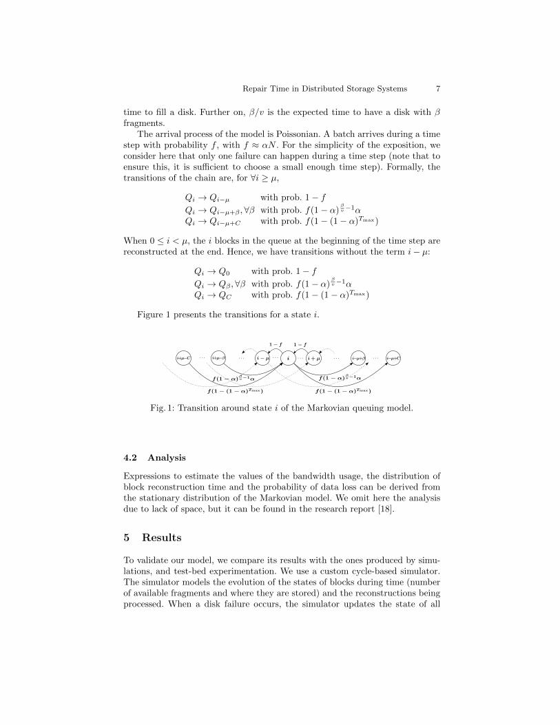
The arrival process of the model is Poissonian. A batch arrives during a timestep with probability f , with f ≈ αN . For the simplicity of the exposition, weconsider here that only one failure can happen during a time step (note that toensure this, it is sufficient to choose a small enough time step). Formally, thetransitions of the chain are, for ∀i ≥ µ,
Qi → Qi−µ with prob. 1− fQi → Qi−µ+β ,∀β with prob. f(1− α)
βv−1α
Qi → Qi−µ+C with prob. f(1− (1− α)Tmax)
When 0 ≤ i < µ, the i blocks in the queue at the beginning of the time step arereconstructed at the end. Hence, we have transitions without the term i− µ:
Qi → Q0 with prob. 1− fQi → Qβ ,∀β with prob. f(1− α)
βv−1α
Qi → QC with prob. f(1− (1− α)Tmax)
Figure 1 presents the transitions for a state i.
Fig. 1: Transition around state i of the Markovian queuing model.
4.2 Analysis
Expressions to estimate the values of the bandwidth usage, the distribution ofblock reconstruction time and the probability of data loss can be derived fromthe stationary distribution of the Markovian model. We omit here the analysisdue to lack of space, but it can be found in the research report [18].
5 Results
To validate our model, we compare its results with the ones produced by simu-lations, and test-bed experimentation. We use a custom cycle-based simulator.The simulator models the evolution of the states of blocks during time (numberof available fragments and where they are stored) and the reconstructions beingprocessed. When a disk failure occurs, the simulator updates the state of all
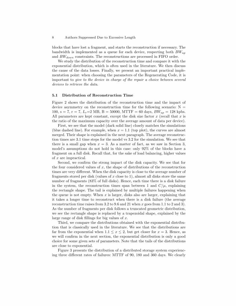
8 Authors Suppressed Due to Excessive Length
blocks that have lost a fragment, and starts the reconstruction if necessary. Thebandwidth is implemented as a queue for each device, respecting both BWup
and BWdown constraints. The reconstructions are processed in FIFO order.We study the distribution of the reconstruction time and compare it with the
exponential distribution, which is often used in the literature. We then discussthe cause of the data losses. Finally, we present an important practical imple-mentation point: when choosing the parameters of the Regenerating Code, it isimportant to give to the device in charge of the repair a choice between severaldevices to retrieve the data.
5.1 Distribution of Reconstruction Time
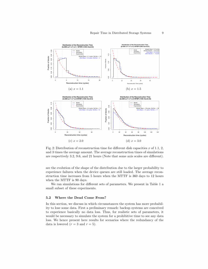
Figure 2 shows the distribution of the reconstruction time and the impact ofdevice asymmetry on the reconstruction time for the following scenario: N =100, s = 7, r = 7, Lr=2 MB, B = 50000, MTTF = 60 days, BWup = 128 kpbs.All parameters are kept constant, except the disk size factor x (recall that x isthe ratio of the maximum capacity over the average amount of data per device).
First, we see that the model (dark solid line) closely matches the simulations(blue dashed line). For example, when x = 1.1 (top plot), the curves are almostmerged. Their shape is explained in the next paragraph. The average reconstruc-tion times are 3.1 time steps for the model vs 3.2 for the simulation. We see thatthere is a small gap when x = 3. As a matter of fact, as we saw in Section 3,model’s assumptions do not hold in this case: only 92% of the blocks have afragment on a full disk. Recall that, for the sake of load balancing, higher valuesof x are impractical.
Second, we confirm the strong impact of the disk capacity. We see that forthe four considered values of x, the shape of distributions of the reconstructiontimes are very different. When the disk capacity is close to the average number offragments stored per disk (values of x close to 1), almost all disks store the samenumber of fragments (83% of full disks). Hence, each time there is a disk failurein the system, the reconstruction times span between 1 and C/µ, explainingthe rectangle shape. The tail is explained by multiple failures happening whenthe queue is not empty. When x is larger, disks also are larger, explaining thatit takes a longer time to reconstruct when there is a disk failure (the averagereconstruction time raises from 3.2 to 9.6 and 21 when x goes from 1.1 to 2 and 3).As the number of fragments per disk follows a truncated geometric distribution,we see the rectangle shape is replaced by a trapezoidal shape, explained by thelarge range of disk fillings for big values of x.
Third, we compare the distributions obtained with the exponential distribu-tion that is classically used in the literature. We see that the distributions arefar from the exponential when 1.1 ≤ x ≤ 2, but get closer for x = 3. Hence, aswe will confirm in the next section, the exponential distribution is only a goodchoice for some given sets of parameters. Note that the tails of the distributionsare close to exponential.
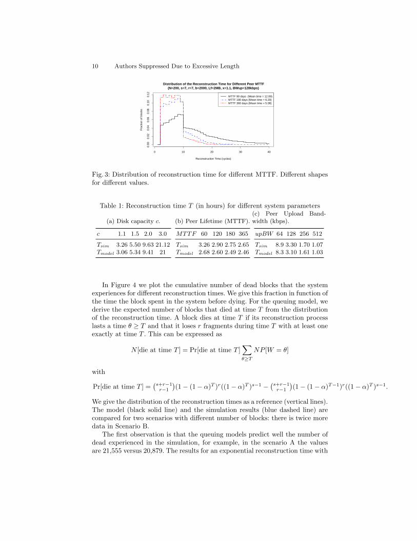
Figure 3 presents the distribution of a distributed storage system experienc-ing three different rates of failures: MTTF of 90, 180 and 360 days. We clearly
Repair Time in Distributed Storage Systems 9
0 5 10 15 20
0.00
0.05
0.10
0.15
0.20
0.25
0.30
Distribution of the Reconstruction Time (b=500 s=7 r=7 x=1.1 MTBF=1440 rho=0.9)
Reconstruction Time (cycles)
Frac
tion
of b
lock
s
(Model) Mean = 3.1 cycles Std.Dev. = 1.8 (Sim) Mean = 3.2 cycles Std.Dev = 2
ModelSimulationExponential
Frac
tion
of b
lock
s
Reconstruction time (cycles)
(a) x = 1.1
0 10 20 30 40
0.00
0.05
0.10
0.15
Distribution of the Reconstruction Time (b=500 s=7 r=7 c=1.5 MTBF=1440 rho=0.67)
Reconstruction Time (cycles)
Fra
ctio
n of
blo
cks
(Model) Mean = 5.3 cycles(Model) Std.Dev. = 3.8 cycles
(Sim) Mean = 5.5 cycles(Sim) Std.Dev. = 4 cycles
ModelSimulationExponential
(b) x = 1.5
0 20 40 60
0.00
0.02
0.04
0.06
0.08
0.10
Distribution of the Reconstruction Time (b=500 s=7 r=7 x=2 MTBF=1440 rho=0.5)
Reconstruction Time (cycles)
Frac
tion
of b
lock
s
(Model) Mean = 9.4 cycles Std.Dev. = 7.4 (Sim) Mean = 9.6 cycles Std.Dev = 7.8
ModelSimulationExponential
Frac
tion
of b
lock
s
Reconstruction time (cycles)
(c) x = 2.0
0 20 40 60 80 100 120 140
0.00
0.01
0.02
0.03
0.04
Distribution of the Reconstruction Time (b=500 s=7 r=7 x=3 MTBF=1440 rho=0.33)
Reconstruction Time (cycles)
Frac
tion
of b
lock
s
(Model) Mean = 28 cycles Std.Dev. = 26 (Sim) Mean = 21 cycles Std.Dev = 17
ModelSimulationExponential
Frac
tion
of b
lock
s
Reconstruction time (cycles)
(d) x = 3.0
Fig. 2: Distribution of reconstruction time for different disk capacities x of 1.1, 2,and 3 times the average amount. The average reconstruction times of simulationsare respectively 3.2, 9.6, and 21 hours (Note that some axis scales are different).
see the evolution of the shape of the distribution due to the larger probability toexperience failures when the device queues are still loaded. The average recon-struction time increases from 5 hours when the MTTF is 360 days to 12 hourswhen the MTTF is 90 days.
We ran simulations for different sets of parameters. We present in Table 1 asmall subset of these experiments.
5.2 Where the Dead Come From?
In this section, we discuss in which circumstances the system has more probabil-ity to lose some data. First a preliminary remark: backup systems are conceivedto experience basically no data loss. Thus, for realistic sets of parameters, itwould be necessary to simulate the system for a prohibitive time to see any dataloss. We hence present here results for scenarios where the redundancy of thedata is lowered (r = 3 and r = 5).
10 Authors Suppressed Due to Excessive Length
0 10 20 30 400.
000.
020.
040.
060.
080.
100.
12
Distribution of the Reconstruction Time for Different Peer MTTF(N=200, s=7, r=7, b=2000, Lf=2MB, x=1.1, BWup=128kbps)
Reconstruction Time (cycles)
Fra
ctio
n of
blo
cks
MTTF 90 days (Mean time = 12.09)MTTF 180 days (Mean time = 6.20)MTTF 360 days (Mean time = 5.08)
Fig. 3: Distribution of reconstruction time for different MTTF. Different shapesfor different values.
Table 1: Reconstruction time T (in hours) for different system parameters
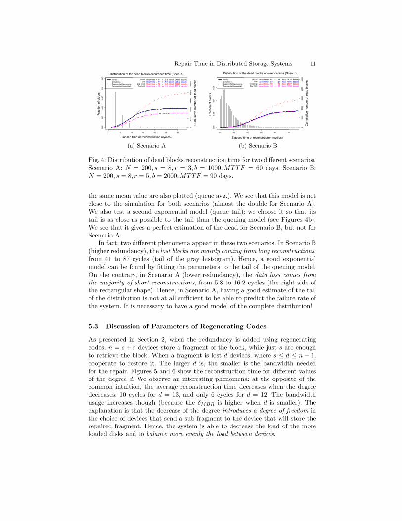
In Figure 4 we plot the cumulative number of dead blocks that the systemexperiences for different reconstruction times. We give this fraction in function ofthe time the block spent in the system before dying. For the queuing model, wederive the expected number of blocks that died at time T from the distributionof the reconstruction time. A block dies at time T if its reconstruction processlasts a time θ ≥ T and that it loses r fragments during time T with at least oneexactly at time T . This can be expressed as
N [die at time T ] = Pr[die at time T ]∑θ≥T
NP [W = θ]
with
Pr[die at time T ] =(s+r−1r−1
)(1− (1− α)T )r((1− α)T )s−1 −
(s+r−1r−1
)(1− (1− α)T−1)r((1− α)T )s−1.
We give the distribution of the reconstruction times as a reference (vertical lines).The model (black solid line) and the simulation results (blue dashed line) arecompared for two scenarios with different number of blocks: there is twice moredata in Scenario B.
The first observation is that the queuing models predict well the number ofdead experienced in the simulation, for example, in the scenario A the valuesare 21,555 versus 20,879. The results for an exponential reconstruction time with
Repair Time in Distributed Storage Systems 11
0 5 10 15 20 25 30
0.00
0.05
0.10
0.15
0.20
0.25
Distribution of the Dead Blocks Occurence Time
Elapsed time of Reconstruction (cycles)
Frac
tion
of B
lock
s
010
000
2000
030
000
4000
050
000
Mean time = 11 +− 5.2 (total 21555 deads) Mean time = 11 +− 4.9 (total 20879 deads) Mean time = 12 +− 6.2 (total 39325 deads) Mean time = 10 +− 5.4 (total 21314 deads)
Distribution of the dead blocks occurence time (Scen. A)
(a) Scenario A
0 20 40 60 80 100
0.00
0.02
0.04
0.06
Distribution of the Dead Blocks Occurence Time
Elapsed time of Reconstruction (cycles)
Frac
tion
of B
lock
s
010
0020
0030
0040
0050
00 Mean time = 64 +− 23 (total 1676 deads) Mean time = 53 +− 21 (total 1696 deads) Mean time = 60 +− 23 (total 2827 deads) Mean time = 56 +− 22 (total 1733 deads)
Distribution of the dead blocks occurence time (Scen. B)
Elapsed time of reconstruction (cycles)
Frac
tion
of b
lock
s
Cum
ulat
ive
num
ber o
f dea
d bl
ocks
Model:Sim:
Exp (avg):Exp (tail):
(b) Scenario B
Fig. 4: Distribution of dead blocks reconstruction time for two different scenarios.Scenario A: N = 200, s = 8, r = 3, b = 1000,MTTF = 60 days. Scenario B:N = 200, s = 8, r = 5, b = 2000,MTTF = 90 days.
the same mean value are also plotted (queue avg.). We see that this model is notclose to the simulation for both scenarios (almost the double for Scenario A).We also test a second exponential model (queue tail): we choose it so that itstail is as close as possible to the tail than the queuing model (see Figures 4b).We see that it gives a perfect estimation of the dead for Scenario B, but not forScenario A.
In fact, two different phenomena appear in these two scenarios. In Scenario B(higher redundancy), the lost blocks are mainly coming from long reconstructions,from 41 to 87 cycles (tail of the gray histogram). Hence, a good exponentialmodel can be found by fitting the parameters to the tail of the queuing model.On the contrary, in Scenario A (lower redundancy), the data loss comes fromthe majority of short reconstructions, from 5.8 to 16.2 cycles (the right side ofthe rectangular shape). Hence, in Scenario A, having a good estimate of the tailof the distribution is not at all sufficient to be able to predict the failure rate ofthe system. It is necessary to have a good model of the complete distribution!
5.3 Discussion of Parameters of Regenerating Codes
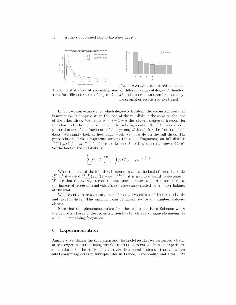
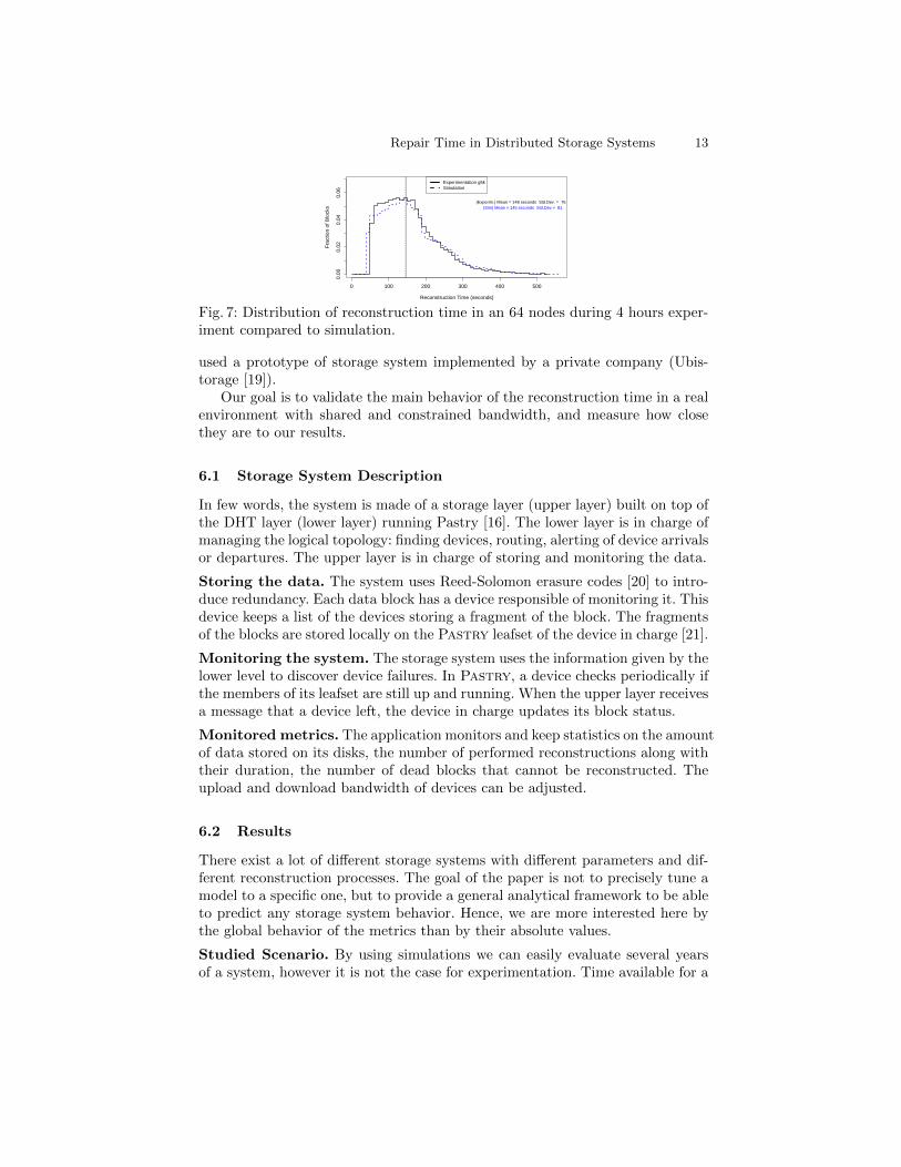
As presented in Section 2, when the redundancy is added using regeneratingcodes, n = s + r devices store a fragment of the block, while just s are enoughto retrieve the block. When a fragment is lost d devices, where s ≤ d ≤ n − 1,cooperate to restore it. The larger d is, the smaller is the bandwidth neededfor the repair. Figures 5 and 6 show the reconstruction time for different valuesof the degree d. We observe an interesting phenomena: at the opposite of thecommon intuition, the average reconstruction time decreases when the degreedecreases: 10 cycles for d = 13, and only 6 cycles for d = 12. The bandwidthusage increases though (because the δMBR is higher when d is smaller). Theexplanation is that the decrease of the degree introduces a degree of freedom inthe choice of devices that send a sub-fragment to the device that will store therepaired fragment. Hence, the system is able to decrease the load of the moreloaded disks and to balance more evenly the load between devices.
12 Authors Suppressed Due to Excessive Length
0 10 20 30 40 50
0.00
0.05
0.10
0.15
Distribution of the reconstruction time for different values of d(N=200, s=7, n=14, b=500, MTBF=60 days)
Reconstruction Time (cycles)
Fra
ctio
n of
blo
cks
[ d=13 ] Mean = 10 cycles [ d=12 ] Mean = 6 cycles [ d=11 ] Mean = 5 cycles
[ d=10 ] Mean = 4.6 cycles
d=13d=12d=11d=10
Fig. 5: Distribution of reconstructiontime for different values of degree d.
13 12 11 10 9 8 7
d
Ave
rage
Rec
onst
ruct
ion
Tim
e (c
ycle
s)
02
46
810 Simulation
10
6
5 4.6 4.3 4.3 4.4
Fig. 6: Average Reconstruction Timefor different values of degree d. Smallerd implies more data transfers, but maymean smaller reconstruction times!
In fact, we can estimate for which degree of freedom, the reconstruction timeis minimum. It happens when the load of the full disks is the same as the loadof the other disks. We define δ = n − 1 − d the allowed degree of freedom forthe choice of which devices upload the sub-fragments. The full disks store aproportion ϕx of the fragments of the system, with ϕ being the fraction of fulldisks. We simply look at how much work we must do on the full disks. Theprobability to have i fragments (among the n − 1 fragments) on full disks is(n−1i
)(ϕx)i(1 − ϕx)n−1−i. Those blocks send i − δ fragments (whenever i ≥ δ).
So the load of the full disks is:
n−1∑i=δ
(i− δ)(n− 1
i
)(ϕx)i(1− ϕx)n−1−i.
When the load of the full disks becomes equal to the load of the other disks(∑n−1i=δ (d − i + δ)
(n−1i
)(ϕx)i(1 − ϕx)n−1−i), it is no more useful to decrease d.
We see that the average reconstruction time increases when d is too small, asthe increased usage of bandwidth is no more compensated by a better balanceof the load.
We presented here a cut argument for only two classes of devices (full disksand non full disks). This argument can be generalized to any number of deviceclasses.
Note that this phenomena exists for other codes like Reed Solomon wherethe device in charge of the reconstruction has to retrieve s fragments among thes+ r − 1 remaining fragments.
6 Experimentation
Aiming at validating the simulation and the model results, we performed a batchof real experimentation using the Grid’5000 platform [4]. It is an experimen-tal platform for the study of large scale distributed systems. It provides over5000 computing cores in multiple sites in France, Luxembourg and Brazil. We
Repair Time in Distributed Storage Systems 13
0 100 200 300 400 500
0.00
0.02
0.04
0.06
Reconstruction Time (seconds)
Fra
ctio
n of
Blo
cks
(Experim.) Mean = 148 seconds Std.Dev. = 76 (Sim) Mean = 145 seconds Std.Dev = 81
Experimentation g5kSimulation
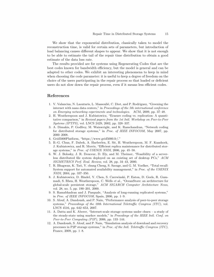
Fig. 7: Distribution of reconstruction time in an 64 nodes during 4 hours exper-iment compared to simulation.
used a prototype of storage system implemented by a private company (Ubis-torage [19]).
Our goal is to validate the main behavior of the reconstruction time in a realenvironment with shared and constrained bandwidth, and measure how closethey are to our results.
6.1 Storage System Description
In few words, the system is made of a storage layer (upper layer) built on top ofthe DHT layer (lower layer) running Pastry [16]. The lower layer is in charge ofmanaging the logical topology: finding devices, routing, alerting of device arrivalsor departures. The upper layer is in charge of storing and monitoring the data.
Storing the data. The system uses Reed-Solomon erasure codes [20] to intro-duce redundancy. Each data block has a device responsible of monitoring it. Thisdevice keeps a list of the devices storing a fragment of the block. The fragmentsof the blocks are stored locally on the Pastry leafset of the device in charge [21].
Monitoring the system. The storage system uses the information given by thelower level to discover device failures. In Pastry, a device checks periodically ifthe members of its leafset are still up and running. When the upper layer receivesa message that a device left, the device in charge updates its block status.
Monitored metrics. The application monitors and keep statistics on the amountof data stored on its disks, the number of performed reconstructions along withtheir duration, the number of dead blocks that cannot be reconstructed. Theupload and download bandwidth of devices can be adjusted.
6.2 Results
There exist a lot of different storage systems with different parameters and dif-ferent reconstruction processes. The goal of the paper is not to precisely tune amodel to a specific one, but to provide a general analytical framework to be ableto predict any storage system behavior. Hence, we are more interested here bythe global behavior of the metrics than by their absolute values.
Studied Scenario. By using simulations we can easily evaluate several yearsof a system, however it is not the case for experimentation. Time available for a
14 Authors Suppressed Due to Excessive Length
simple experiment is constrained to a few hours. Hence, we define an accelerationfactor, as the ratio between experiment duration and the time of real systemwe want to imitate. Our goal is to check the bandwidth congestion in a realenvironment. Thus, we decided to shrink the disk size (e.g., from 10 GB to 100MB, a reduction of 100×), inducing a much smaller time to repair a failed disk.Then, the device failure rate is increased (from months to a few hours) to keepthe ratio between disk failures and repair time proportional. The bandwidthlimit value, however, is kept close to the one of a “real” system. The idea is toavoid inducing strange behaviors due to very small packets being transmitted inthe network.
4000 5000 6000 7000 8000 9000 10000 11000
050
010
0015
0020
00
Timeseries of the Reconstructions in Queue (Experimentation)
Time (seconds)
Que
ue L
engt
h (fr
agm
ents
)
Timeseries of number of reconstructions in queue (Experimentation)
Time (seconds)
Que
ue le
ngth
(fra
gmen
ts)
4000 5000 6000 7000 8000 9000 10000 110000.
00.
20.
40.
60.
81.
0
Upload Bandwidth Consumption over Time (Experimentation)
Time (seconds)
Rat
io o
f Ban
dwid
th U
sage
(rho
)
Mean rho = 0.78
Timeseries of the upload bandwidth consumption (Experimentation)
Frac
tion
of B
W u
sage
(rho
)Time (seconds)
Fig. 8: Time series of the queue size (left) and the upload bandwidth ratio (right).
Figure 7 presents the distribution of the reconstruction times for two differ-ent experimentation involving 64 nodes on 2 different sites of Grid’5000. Theamount of data per node is 100 MB (disk capacity 120MB), the upload band-width 128 KBps, s = 4, r = 4, LF = 128 KB. We confirm that the simulatorgives results very close to the one obtained by experimentation. The averagevalue of reconstruction time differs by a few seconds.
Moreover, to have an intuition of the system dynamics over time, in Figure 8we present a time series of the number of blocks in the queues (top plot) andthe total upload bandwidth consumption (bottom plot). We note that the rateof reconstructions (the descending lines on the top plot) follows an almost linearshape. Comforting our claim that a deterministic processing time of blocks couldbe assumed. In these experiments the disk size factor is x = 1.2, which givesa theoretical efficiency of 0.83. We can observe that in practice, the factor ofbandwidth utilization, ρ, is very close to this value (value of ρ = 0.78 in thebottom plot).
7 Conclusions and take-aways
In this paper, we propose and analyze a new Markovian analytical model tomodel the repair process of distributed storage systems. This model takes intoaccount competition for bandwidth between correlated failures. We bring tolight the impact of device heterogeneity on the system efficiency. The model isvalidated by simulation and by real experiments on the Grid’5000 platform.
We show that load balancing in storage is crucial for reconstruction time. Weintroduce a simple linear factor of efficiency, where throughput of the system isdivided by the ratio of maximum allowed disk size to the average occupancy.
Repair Time in Distributed Storage Systems 15
We show that the exponential distribution, classically taken to model thereconstruction time, is valid for certain sets of parameters, but introduction ofload balancing causes different shapes to appear. We show that it is not enoughto be able to estimate the tail of the repair time distribution to obtain a goodestimate of the data loss rate.
The results provided are for systems using Regenerating Codes that are thebest codes known for bandwidth efficiency, but the model is general and can beadapted to other codes. We exhibit an interesting phenomena to keep in mindwhen choosing the code parameter: it is useful to keep a degree of freedom on thechoice of the users participating in the repair process so that loaded or deficientusers do not slow down the repair process, even if it means less efficient codes.
References
1. V. Valancius, N. Laoutaris, L. Massoulie, C. Diot, and P. Rodriguez, “Greening theinternet with nano data centers,” in Proceedings of the 5th international conferenceon Emerging networking experiments and technologies. ACM, 2009, pp. 37–48.
2. H. Weatherspoon and J. Kubiatowicz, “Erasure coding vs. replication: A quanti-tative comparison,” in Revised papers from the 1st Intl. Workshop on Peer-to-PeerSystems (IPTPS), vol. LNCS 2429, 2002, pp. 328–337.
3. A. Dimakis, P. Godfrey, M. Wainwright, and K. Ramchandran, “Network codingfor distributed storage systems,” in Proc. of IEEE INFOCOM, May 2007, pp.2000–2008.
4. Grid5000Platform, “https://www.grid5000.fr/.”5. B.-G. Chun, F. Dabek, A. Haeberlen, E. Sit, H. Weatherspoon, M. F. Kaashoek,
J. Kubiatowicz, and R. Morris, “Efficient replica maintenance for distributed stor-age systems,” in Proc. of USENIX NSDI, 2006, pp. 45–58.
6. W. J. Bolosky, J. R. Douceur, D. Ely, and M. Theimer, “Feasibility of a server-less distributed file system deployed on an existing set of desktop PCs,” ACMSIGMETRICS Perf. Eval. Review, vol. 28, pp. 34–43, 2000.
7. R. Bhagwan, K. Tati, Y. chung Cheng, S. Savage, and G. M. Voelker, “Total recall:System support for automated availability management,” in Proc. of the USENIXNSDI, 2004, pp. 337–350.
8. J. Kubiatowicz, D. Bindel, Y. Chen, S. Czerwinski, P. Eaton, D. Geels, R. Gum-madi, S. Rhea, H. Weatherspoon, C. Wells et al., “OceanStore: an architecture forglobal-scale persistent storage,” ACM SIGARCH Computer Architecture News,vol. 28, no. 5, pp. 190–201, 2000.
9. S. Ramabhadran and J. Pasquale, “Analysis of long-running replicated systems,”in Proc. of IEEE INFOCOM, Spain, 2006, pp. 1–9.
10. S. Alouf, A. Dandoush, and P. Nain, “Performance analysis of peer-to-peer storagesystems,” Proceedings of the 20th International Teletraffic Congress (ITC), vol.LNCS 4516, pp. 642–653, 2007.
11. A. Datta and K. Aberer, “Internet-scale storage systems under churn – a study ofthe steady-state using markov models,” in Procedings of the IEEE Intl. Conf. onPeer-to-Peer Computing (P2P), 2006, pp. 133–144.
12. A. Dandoush, S. Alouf, and P. Nain, “Simulation analysis of download and recoveryprocesses in P2P storage systems,” in Proc. of the Intl. Teletraffic Congress (ITC),France, 2009, pp. 1–8.
16 Authors Suppressed Due to Excessive Length
13. F. Picconi, B. Baynat, and P. Sens, “Predicting durability in dhts using markovchains,” in Proceedings of the 2nd Intl. Conference on Digital Information Man-agement (ICDIM), vol. 2, Oct. 2007, pp. 532–538.
14. V. Venkatesan, I. Iliadis, and R. Haas, “Reliability of data storage systems undernetwork rebuild bandwidth constraints,” in Modeling, Analysis & Simulation ofComputer and Telecommunication Systems (MASCOTS), 2012 IEEE 20th Inter-national Symposium on. IEEE, 2012, pp. 189–197.
15. D. Ford, F. Labelle, F. I. Popovici, M. Stokely, V.-A. Truong, L. Barroso,C. Grimes, and S. Quinlan, “Availability in globally distributed storage systems,”in Proceedings of the 9th USENIX conference on Operating systems design andimplementation. USENIX Association, 2010, pp. 1–7.
16. A. Rowstron and P. Druschel, “Pastry: Scalable, decentralized object location, androuting for large-scale peer-to-peer systems,” in Proc. of IFIP/ACM Intl. Conf. onDistributed Systems Platforms (Middleware), vol. LNCS 2218, 2001, pp. 329–350.
17. “Planetlab.” [Online]. Available: http://www.planet-lab.org/18. F. Giroire, S. Gupta, R. Modrzejewski, J. Monteiro, and S. Perennes, “Analysis
of the repair time in distributed storage systems,” INRIA, Tech. Rep. 7538, Feb.2011.
19. “Ubistorage,” http://www.ubistorage.com/.20. M. Luby, M. Mitzenmacher, M. Shokrollahi, D. Spielman, and V. Stemann, “Prac-
tical loss-resilient codes,” in Proceedings of the 29th annual ACM symposium onTheory of computing, 1997, pp. 150–159.
21. S. Legtchenko, S. Monnet, P. Sens, and G. Muller, “Churn-resilient replicationstrategy for peer-to-peer distributed hash-tables,” in Proceedings of SSS, vol. LNCS5873, 2009, pp. 485–499.