Repairing wireless sensor network connectivity with mobility and hop-count constraints Thuy T. Truong, Kenneth N. Brown and Cormac J. Sreenan Mobile & Internet Systems Laboratory and Cork Constraint Computation Centre, Department of Computer Science, University College Cork, Ireland Email: {tt11, k.brown, cjs}@cs.ucc.ie Abstract. Wireless Sensor Networks can become partitioned due to node failure or damage, and must be repaired by deploying new sen- sors, relays or sink nodes to restore some quality of service. We formu- late the task as a multi-objective problem over two graphs. The solution specifies additional nodes to reconnect a connectivity graph subject to network path-length constraints, and a path through a mobility graph to visit those locations. The objectives are to minimise both the cost of the additional nodes and the length of the mobility path. We propose two heuristic algorithms which prioritise the different objectives. We eval- uate the two algorithms on randomly generated graphs, and compare their solutions to the optimal solutions for the individual objectives. Fi- nally, we assess the total restoration time for different classes of agent, i.e. small robots and larger vehicles, which allows us to trade-off longer computation times for shorter mobility paths. Keywords: Sensor Network, Connectivity Repair, Sink Placement 1 Introduction Wireless Sensor Networks are becoming increasingly important for monitoring phenomena in remote or hazardous environments, including pollution monitor- ing, chemical process sensing, disaster response, and battlefield monitoring. As these environments are uncontrolled and may be volatile, the network may suf- fer damage, from hazards, direct attack or accidental damage from wildlife and weather. They may also degrade through battery depletion or hardware failure. The failure of an individual sensor node may mean the loss of particular data streams generated by that node; more significantly, node failure may partition the network, meaning that many data streams cannot be transmitted to the sink. This creates the network repair problem, in which we must place new radio nodes in the environment to restore connectivity to the sink for all sub-partitions. In this work, we assume a survey has been completed, and so we know which nodes have failed, which radio links have been blocked, and which routes between positions can no longer be traversed. The tasks that remain are to decide on the positions for the new radio nodes, and to plan and follow a route through the environment to place those nodes. We assume possible locations for new radio
Transcript
Repairing wireless sensor network connectivitywith mobility and hop-count constraints
Thuy T. Truong, Kenneth N. Brown and Cormac J. Sreenan
Mobile & Internet Systems Laboratory and Cork Constraint Computation Centre,Department of Computer Science, University College Cork, Ireland
Email: {tt11, k.brown, cjs}@cs.ucc.ie
Abstract. Wireless Sensor Networks can become partitioned due tonode failure or damage, and must be repaired by deploying new sen-sors, relays or sink nodes to restore some quality of service. We formu-late the task as a multi-objective problem over two graphs. The solutionspecifies additional nodes to reconnect a connectivity graph subject tonetwork path-length constraints, and a path through a mobility graph tovisit those locations. The objectives are to minimise both the cost of theadditional nodes and the length of the mobility path. We propose twoheuristic algorithms which prioritise the different objectives. We eval-uate the two algorithms on randomly generated graphs, and comparetheir solutions to the optimal solutions for the individual objectives. Fi-nally, we assess the total restoration time for different classes of agent,i.e. small robots and larger vehicles, which allows us to trade-off longercomputation times for shorter mobility paths.
Wireless Sensor Networks are becoming increasingly important for monitoringphenomena in remote or hazardous environments, including pollution monitor-ing, chemical process sensing, disaster response, and battlefield monitoring. Asthese environments are uncontrolled and may be volatile, the network may suf-fer damage, from hazards, direct attack or accidental damage from wildlife andweather. They may also degrade through battery depletion or hardware failure.The failure of an individual sensor node may mean the loss of particular datastreams generated by that node; more significantly, node failure may partitionthe network, meaning that many data streams cannot be transmitted to the sink.This creates the network repair problem, in which we must place new radio nodesin the environment to restore connectivity to the sink for all sub-partitions.
In this work, we assume a survey has been completed, and so we know whichnodes have failed, which radio links have been blocked, and which routes betweenpositions can no longer be traversed. The tasks that remain are to decide on thepositions for the new radio nodes, and to plan and follow a route through theenvironment to place those nodes. We assume possible locations for new radio
2 Thuy T. Truong, Kenneth N. Brown and Cormac J. Sreenan
nodes are limited to a finite set of positions where a node can be securely placedand which can be accessed. Radio nodes are expensive, and so solutions whichrequire fewer nodes are preferred. In addition, the users of the WSN may requiredata to be transmitted from the sensors quickly, to allow a timely response,and so there will be limits on the number of radio hops allowed between thesensors and the wider network. To achieve this, we may prefer to deploy someexpensive sink nodes which provide their own network connection, in additionto relay nodes. Physically moving around the environment may be expensivein energy use, may take significant time, or may expose the agent placing thenodes to danger, and so solutions which allow cheaper path plans are also pre-ferred. Depending on the application, either one of the two objectives may bemore important: placing expensive nodes in, for example, agricultural pollutionmonitoring favours solutions with fewer nodes, while restoring connectivity dur-ing disaster response favours solutions that can be deployed quickly even if theyrequire more nodes. Thus the network repair problem is multi-objective.
We introduce the problem of simultaneous network repair with hop countlimits and route planning with limited mobility. We assume a set of desiredlocations from which sensor data is required by the network, and we assume theagent knows the state of the network and accessibility. The objective is to connectas many as possible of these locations, placing extra sensors, relays and sinksas required, minimising the relay and sink costs and the mobility costs, whileobeying the constraint on the number of allowed radio hops. We consider twodifferent heuristic approaches for the multi-objective problem, each prioritisinga different objective: minimising mobility costs, and minimising the relay andsink costs. We evaluate the two algorithms on randomly generated problems,and analyse their effectiveness under different assumptions. Finally, we considerthe total estimated time to restore the network, for two different classes of agent(a small robot and a larger vehicle), and we show that the choice of priorityshould be dependent on the performance of the agent.
2 The Network Repair Problem
Given a damaged sensor network and set of terminal locations from which werequire sensed data, our goal is to place new nodes to ensure that each terminal isconnected to a sink within a given number of radio links, and to find a mobilitypath through the environment to place the nodes, while minimising both thecost of the radio nodes and the length of the path.
Let V be a set of possible radio locations. Ec⊆V×V is the set of possible radiolinks, Em⊆V×V is a set of traversable edges, and w:Em→N specifies the lengthof each edge. A path p in graph G=(V,E) is a sequence [x1, x2, x3, . . . , xk−1, xk]where each {xi, xi+1}∈E. The hop count of a path in the connectivity graphGc=(V,Ec) is one less than the number of nodes in the path, while the lengthof a path p in the mobility graph Gm=(V,Em) is
∑(xi,xi+1)∈p w({xi, xi+1}). Lr
is the set of locations with existing relay (and sensor) nodes, while Ls is the setof locations with existing sink (and sensor) nodes. T is the set of terminal nodes
Repairing WSN connectivity with mobility and hop-count constraints 3
which must be reconnected within the hop count limit k, and α∈V is the initialstarting location of our agent. cr is the cost of a relay node, while cs is the costof a sink node. The problem is to find two new subsets R⊆V and S⊆V of relaynodes and sink nodes, such that for each terminal t∈T there is a sink s∈S anda path through the connectivity graph (Lr∪Ls∪R∪S,Ec) to s with a hop count≤k, and a tour p in the mobility graph Gm that starts and finishes at α and visitseach element of R∪S, which minimises the pair (length(p), (|R| ∗ cr)+(|S| ∗ cs))of the mobility tour length and the node cost.
Note that the two objectives may conflict. As an example, Figure 1 shows (a)a connectivity graph and (b) a mobility graph for a set of terminals T={t1, t2, t3}and a set of candidate locations {a,b,d,e,f,g,h,j}. Assuming cs=3∗cr, k=2 and thecurrent location of the agent is at f , a minimal cost node deployment to reconnectall terminals within a hop count limit of 2 is S={d, t3}, R={t1}, with cost 7∗ cr.The shortest path in the mobility graph is [f, t3, f, e, b, h, t1, h, a, d, a, e, f ] withlength 45. For a deployment of S={t1, t3, g}, R={}, the node cost is 9 ∗ cr, butthere is a path [f, g, f, t3, f, e, b, h, t1, h, b, e, f ] with length 34. Which of thesesolutions should be selected will depend on the relative cost of the sink andradio nodes compared to the cost of traversing the path. High node costs andlow mobility costs will prefer the first solution, while high mobility costs willprefer the second solution.
(a) Connectivity Graph (b) Mobility Graph
h
a
d
b
e
f
gjt2
t1
t3
2
2 h
a
d
b
e
f
gj
6
3
34
82
2
2
t1
t2
5
t3
candidate position
candidate positionwith live node
terminal
terminal with live node
agent’s location
Fig. 1. Example Network Repair Problem
The objective of minimising the mobility path length has a travelling sales-man path problem embedded inside it, and so we choose to investigate heuristicapproaches. To address the two objectives, we consider two approaches, whicheach prioritise one of the objectives.
3 The Node Optimisation Heuristic Algorithm
Our first approach prioritises the node cost, by searching for a low cost setof relay and sink nodes which connect the terminals to sinks within the hopcount limit (Algorithm 1). Given a set of nodes, we then search for the cheapestmobility path that visits those nodes (Algorithm 2). We start by finding, for eachterminal j the set Tj of all possible sink locations (i.e. locations within k hops
4 Thuy T. Truong, Kenneth N. Brown and Cormac J. Sreenan
of j in the connectivity graph). For each sink location si which is associatedwith two or more terminals, we determine the valuation (xi, yi), where xi isthe number of terminals which could be connected by si, and yi is an upperbound on the number of new relay nodes that would be required to connectthem. The set O={si|xi∗cs≥cs+yi∗cr} then contains all such sinks that couldconnect all of their terminals for less than the cost of placing a separate sinkfor each terminal. We order O by the expected total cost of deploying that sink,(|T |−xi)∗cs + yi∗cr + cs, where yi∗cr + cs is the cost of placing that sink withextra radio nodes yi to reconnect the expected xi terminals, and (|T |−xi)∗cs isan upper bound on the cost of placing sinks at the remaining terminals in T . Wethen select the first sink location in O, add it to S, the set of new sinks, computerelay node locations to connect the terminals and add them to R, the new relays.We then recompute the valuations and reorder the set O to reflect the changesin the unconnected terminals, and repeat. Once O is empty, for each remainingunconnected terminal j we place a sink at a random location in Tj . The mostexpensive operation is the calculation of (xi, yi) where we use a best-first searchto find the shortest connectivity path from a terminal to each location si ∈ O,and we re-use those paths when we select the relay node locations.
For the problem of finding a short tour for the selected nodes (Algorithm2), we create from the mobility graph Gm a metric closure graph for the newnodes in S∪R. We then apply [1]’s Greedy-TSP heuristic - we sort the edges inincreasing order of cost, and we iteratively add the lowest cost edge which doesnot increase any vertex’s degree to 3, and which does not create a cycle unless itcompletes the tour. The runtime is dominated by the time of building the metricclosure graph, i.e. O(|S∪R|∗|V |2).
Figure 2 shows the NOH algorithm being applied to the example of Figure1. First we find all sets Tj for each j∈T (Figure 2(a)). We then find and orderthe set O (b). We select the first entry in O for a sink node, and it requires oneadditional relay node at t1 (c). As t1 and t2 now have a connection to the sink atd within 2 hops, we remove them from the list T . Now a connects no terminalsin T , while b and g only connect one terminal t3. Therefore, we remove them allfrom the list O and terminate the while loop. We then select t3 for a new sink (d)and finish the algorithm. Finally, we apply Greedy TSP to find a tour visitingthose selected locations, giving P = [f, t3, f, e, b, h, t1, h, a, d, a, e, f ] which costs45 units for 2 sinks and 1 relay node.
4 The Path Optimisation Heuristic Algorithm
Our second approach prioritises the mobility cost. First, for each terminal j∈T ,we find the set Cj of all locations within the hop count limit from j but thatrequire at most one extra node to connect j. Since we must guarantee connec-tivity within k hops for each terminal, we must place at least one node in eachCj . Placing a sink node in Cj ensures that no other node is required in Cj . Sincethe aim is to minimise mobility cost, we now search for a set of nodes that coverthe Cj and which can be visited with the shortest possible tour.
Repairing WSN connectivity with mobility and hop-count constraints 5
Algorithm 1: Node Selection
Data: Gc=(V,Ec), Gm=(V,Em), Ls, Lr, T , kResult: S (new sinks), R (new relays)begin
foreach j in T doFind the set Tj⊆V within k hops of j in Gc
O={}foreach oi in more than one Tj do
Compute the values (xi, yi)if cs ∗ xi≥cr ∗ yi + cs then
add oi to O in increasing order of (|T |−xi)∗cs + yi∗cr + cs
while O and T are not empty doMove first oi from O into Sforeach j∈T such that oi∈Tj do
Find connectivity path p for oi to jforeach location l in p not in Ls∪Lr do
add l into R
Remove j from T
Re-calculate (xi, yi) for all affected entries in Oforeach oj ∈ O with xj=1 do
Remove oj from O
Re-order O
foreach j ∈ T doselect a location l from Tj and add to S
Algorithm 2: GreedyTour
Data: A set of vertices V ′, a graph GM = (V,EM )Result: a tour in GM visiting all nodes in V ′
j∈T Cj , and E′={{u, v}|u∈Ci,v∈Cj , i6=j}, i.e. the graph of locations in the cluster sets Cj with an edge be-tween every pair of locations from different cluster sets. We associate a weightto each edge in E′ equal to the shortest path length in Gm between the twoendpoints. Note that any location which appears in two cluster sets will have a0-weighted self-edge. The path optimisation problem can now be modeled as aGeneralized Travelling Salesman Problem (GTSP) on G where the agent needsto visit exactly one node in each cluster Ci ([2]). We use the memetic algorithmfor the GTSP proposed by Gutin and Karapetyan in [3]. The algorithm cre-
6 Thuy T. Truong, Kenneth N. Brown and Cormac J. Sreenan
(a) (b) (c) (d) (e)h
a
d
b
e
f
gj
t2
t1
t3
T1={t1,h,a,d,b}, T2={t2,a,d,j,g},T3={t3,b,e,f,g}
T1
T2 T3
h
a
d
b
e
f
g
j
t2
t1
t3
T={t1,t2,t3}, O={d, a, g, b},fd=<2,1>, fa=<2,2>,fg=<2,2>, fb=<2,4>
T1
T2
T3
h
a
d
b
e
f
gj
t2
t1
t3
- Select d for new sink-> t1 for radio- t1, t2 connected to sink d: T={t3}- Remove a, b, g from O as they areno longer in overlapped area
h
a
d
b
e
f
gj
t2
t1
t3
- Select t3 for new sink.- Result: 2 sinks at d and t3
and 1 radio node at t1.
2
2 h
a
d
b
e
f
gj
2
3
34
72
22
t1
t2
5
t3
Tour: f-t3-f-e-b-h-t1-h-a-d-a-e-f with 45
units.
Fig. 2. A sample execution of NOH
ates a first generation of 2∗|T | tours by creating random permutations of theclusters and then finds the best vertex in each cluster using the Cluster Optimi-sation Heuristic (CO). The CO heuristic uses the shortest (s, t)-path for acyclicdigraphs to find the best vertex for each cluster when the order of clusters isfixed (see [4]). It then runs a local improvement procedure on each solution.The procedure runs several local search heuristics sequentially including Swaps(swap every non-neighboring pair of vertices), k-Neighbor Swap (try all the per-mutations which are not covered by any of i-Neighbor Swap, i = 2, 3, ..., k − 1),2-opt (try to replace every non-adjacent pair of edges (si, si+1) and (sj , sj+1) bythe edges (si, sj) and (si+1, sj+1)), Direct 2-opt (a modification of 2-opt, whichonly selects some of the longest edges in the solution), and Insert (remove avertex from the solution and insert it in different position). The procedure ap-plies all those local search heuristics in a loop, removing any heuristic that failsto improve the solution. Once the loop terminates, it applies the CO heuristicagain, and stops. The next generation is created by reproduction, crossover, andmutation operators applied in parallel to the previous generation. Reproductionsimply copies the best solutions from the previous generation. The crossover op-erator is a 2-point crossover producing a single child, by selecting a fragmentfrom the first parent, and then completes the tour by copying the order of the2nd parent’s nodes starting with the node at the end of the selected fragment,and deleting any repeated nodes. The parents are selected randomly from thetop 33% of individuals. The mutation operator modifies each selected parent(selected from the top 75%) by removing a random fragment and inserting itrandomly in a new position. Reproduction, crossover and mutation generate newchildren in the ratio (1 : 8 : 2). The local improvement moves are then appliedto each individual. The algorithm repeats until a time limit is reached. Whenrunning the algorithm in the experiments, we use the same parameter valuesgiven in [3]. Note that the overall running time is dominated by the creation ofthe initial weighted graph.
The memetic algorithm results in a sequence of locations to be visited, andwe obtain a feasible solution if we place a sink at each location. We now improvethat solution by replacing as many sinks with relay nodes as possible (Algorithm4). We start by assuming all locations in the set are occupied by relay nodes.
Repairing WSN connectivity with mobility and hop-count constraints 7
Algorithm 3: Memetic Algorithm
Data: G = (V ′, E′) (graph), a set of clusters Ci, i∈TResult: a tour visiting exactly one node in each Ci
beginInitialize, construct first generation of solutions;Improve the first generation by local search, eliminate duplicate solutions;while not termination condition do
Produce next generation by genetic operators (reproduction, crossover,mutation);Improve the next generation by local search, eliminate duplicatesolutions;
We order the set in decreasing order of the number of terminals within k hopsof each location. We select the first location, convert it into a sink, and removefrom T all terminals connected to that sink in ≤ k hops. We repeat until T isempty. Any locations remaining in N are left as relay nodes.
Algorithm 4: Node Selection Algorithm
Data: N (set of locations), Gc = (Ls∪Lr∪N,Ec) (graph), T (set of terminals)Result: S (locations for sinks), R (locations for relays)begin
S←{};while T is not empty do
Sort N in decreasing order of number of j∈T within k hops in Gc;Move first element n0 from N to S;Remove all j from T where j is connected to n0 within k hops in Gc;
R←N
Figure 3 shows the POH algorithm being applied to the example of Figure1. First, we find a set of clusters for each terminal in Gc (Figure 3(a)). We thencalculate the costs of moving from each node in each cluster to other nodesin different clusters (b). We apply the memetic algorithm to this new graphand it produces the tour [f, t3, g, t1, f ] (c) which is then mapped into Gm asP=[f, t3, f, g, f, e, b, h, t1, h, b, e, f ] with a mobility cost of 34 (d). Finally, weapply the Node Selection algorithm in Gc for those visited locations {t1, t3, g}which results in 3 new sinks.
5 Evaluation
Both proposed algorithms (NOH and POH) are heuristic, and take differentapproaches to the multi-objective problem. Therefore, we evaluate them empir-ically on randomly generated graphs, to compare the quality of their solutions
8 Thuy T. Truong, Kenneth N. Brown and Cormac J. Sreenan
(a) (b) (c) (d) (e)h
a
d
b
e
f
gjt2
t1
t3
C1={t1}, C2={t2,j,d, g}, C3={t3}, C0={f}
C1
C3
C2
C0
df
jt2
t1
t3
C1={t1}, C2={t2,j,d,g}, C3={t3}, C0={f}
C1
C3
C2
101619
17 14
279
911
16
g
15
8
df
jt2
t1
t3
The memetic result:f-t3-g-t1-f
C1
C3
C2
101619
17 14
279
911
16
g
15
7
2
2 h
a
d
b
e
f
gj
6
3
34
82
22
t1
t2
5
t3
Result in GM: f-t3-f-g-f-e-b-h-t1-h-b-e-f with
34 units
h
a
d
b
e
f
gjt2
t1
t3
The Node Selection result: 3 sinks at t1, t3
and g
Fig. 3. A sample execution of POH
on both objectives, and also on their runtime. For the graphs, our aim is torepresent a physical area rather than abstract random graphs, and so we use agrid to generate the graphs. Connectivity is based on the distance between twolocations. To represent a landscape or a building interior, we add obstacles intothe grid, which may hinder or forbid access. The mobility graph is then basedon line-of-sight, with some limited ability to cross the obstacles.
We generate graphs within a rectangular area consisting of n×m squares ofsize 10 units. Within this space, we place o mobility obstacles, where each ob-stacle is a random polygon contained within a randomly selected pair of neigh-bouring cells. For each square, we generate a random position within it; if thatposition is inside an obstacle, we discard it, otherwise we designate it as a can-didate location. Each obstacle is given a random weight w between 0 and 1,representing the difficulty it creates for the agent to traverse it, and such thatany obstacle with a weight greater than 0.2 is assumed not able to be traversed.
We then create the connectivity graph by adding edges indicating that twocandidate locations are within transmission range. For each pair of locations, weadd with probability 0.85 an edge if they are within 10 units apart; we add withprobability 0.2 an edge for each pair of locations which is between 10 and 20units apart. This is to simulate the radio obstacles where we don’t have uniformcommunication ranges. For the mobility graph, we add an edge between any pairof locations which are less than 25 units apart and which can be connected by astraight line that does not cross an obstacle. The weight of the edge is simply thelength of the connecting line. For any pair of locations separated by a distanceof less than 25 and which has a straight line that traverses all obstacle with aweight less than or equal to 0.2, we add those edges into the mobility graph. Thecost of the edge is the distance plus 10*weight for each obstacle it crosses.
We consider the problem size: (i) a 10 × 10 grid, and thus a maximumof 100 candidate locations, and 20 possible obstacles1. We perform two sets ofexperiments: varying the number of terminals and varying the hop count limit k.For each data point, we generate 50 instances, and present the average solution
1 We also experimented with the problem size 5 × 10 grid, and thus a maximum of50 candidate locations, and 10 possible obstacles, and got similar results.
Repairing WSN connectivity with mobility and hop-count constraints 9
cost (mobility cost, number of nodes needed) and runtime. For each instance,we randomly select candidate locations as terminals or live nodes. Finally, wecalculate the total time to restore the network for different agent speeds, bycombining the runtime with the estimated travel time.
To assess the quality of the solutions, we compare the results against the op-timal solutions for each individual objective, generated by an exhaustive search.That is, OPT-N first finds the set of sinks and relay nodes with lowest costthat connect all the terminals with the hop count. For that set, a tour is thengenerated using Algorithm 2. OPT-P first generates the optimal mobility tourthat could connect all terminals within the hop count (by selecting the optimaltour that visits each cluster set). For the locations on the tour, we then selectthe locations to be used as sinks using Algorithm 4.
First, we vary the number of terminals and fix the hop count limit as k = 2.Figure 4 shows the number of nodes placed by each algorithm. As the numberof terminals to be connected increases, the node cost rises as expected. The twoalgorithms that prioritise mobility incur 25% higher node costs than their nodeequivalents. The mobility costs rise as we increase the number of terminals. Theheuristic POH is within 30% of the exact OPT-P. As above, the algorithms thatprioritise node cost create approximately 40% higher mobility costs.
0
2
4
6
8
10
12
14
16
4 5 6 7
no
de
co
st (
*cn
)
number of terminals
Node cost with different number of terminals.
NOH
POH
N-OPT
P-OPT
150
200
250
300
350
400
450
4 5 6 7
mo
bil
ity
co
st
Mobility cost with different number of terminals.
NOH
POH
N-OPT
P-OPT
Fig. 4. Varying number of terminals
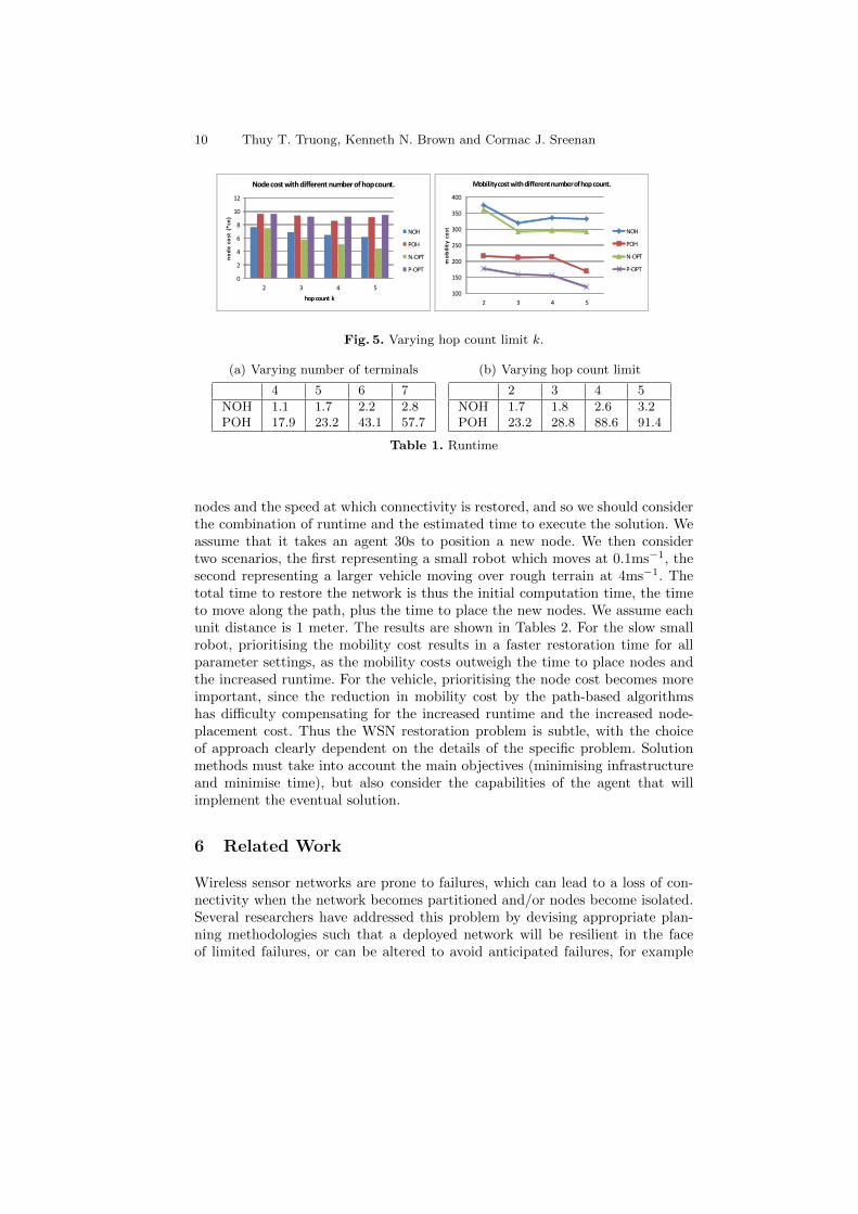
In the second set of the experiments, we fix the number of terminals at 5, andvary the hop count limit k. As the hop limit increases, the node costs decrease,as the connectivity problem becomes easier (Figure 5). The performance gapbetween the node-based algorithms and the path-based algorithms increases.The mobility costs also decrease as the hop limit increases. We believe this isbecause the reduction in the cost is due to placing a small number of sinks inthe centre of the map, thus requiring a shorter path to visit those locations.
Table 1 shows the runtimes for the algorithms in both experiments. All in-crease with the number of terminals and the hop count k. The running time ofNOH is significantly faster that of POH due to POH takes time to compute theclusters and path cost between clusters.
Finally, we note that the mobility costs are associated only with the distancetravelled. For real scenarios, there is a tradeoff between the cost of the extra
10 Thuy T. Truong, Kenneth N. Brown and Cormac J. Sreenan
0
2
4
6
8
10
12
2 3 4 5
no
de
co
st (
*cn
)
hop count k
Node cost with different number of hop count.
NOH
POH
N-OPT
P-OPT
100
150
200
250
300
350
400
2 3 4 5
mo
bil
ity
co
st
Mobility cost with different number of hop count.
NOH
POH
N-OPT
P-OPT
Fig. 5. Varying hop count limit k.
(a) Varying number of terminals
4 5 6 7
NOH 1.1 1.7 2.2 2.8POH 17.9 23.2 43.1 57.7
(b) Varying hop count limit
2 3 4 5
NOH 1.7 1.8 2.6 3.2POH 23.2 28.8 88.6 91.4
Table 1. Runtime
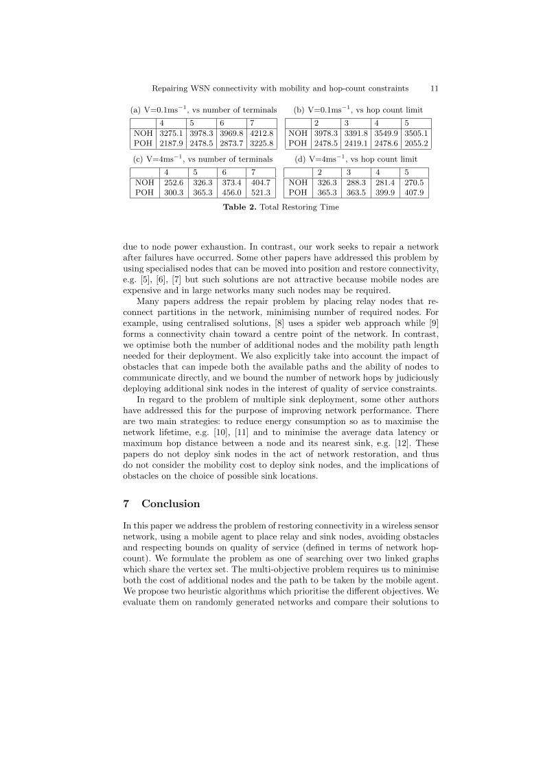
nodes and the speed at which connectivity is restored, and so we should considerthe combination of runtime and the estimated time to execute the solution. Weassume that it takes an agent 30s to position a new node. We then considertwo scenarios, the first representing a small robot which moves at 0.1ms−1, thesecond representing a larger vehicle moving over rough terrain at 4ms−1. Thetotal time to restore the network is thus the initial computation time, the timeto move along the path, plus the time to place the new nodes. We assume eachunit distance is 1 meter. The results are shown in Tables 2. For the slow smallrobot, prioritising the mobility cost results in a faster restoration time for allparameter settings, as the mobility costs outweigh the time to place nodes andthe increased runtime. For the vehicle, prioritising the node cost becomes moreimportant, since the reduction in mobility cost by the path-based algorithmshas difficulty compensating for the increased runtime and the increased node-placement cost. Thus the WSN restoration problem is subtle, with the choiceof approach clearly dependent on the details of the specific problem. Solutionmethods must take into account the main objectives (minimising infrastructureand minimise time), but also consider the capabilities of the agent that willimplement the eventual solution.
6 Related Work
Wireless sensor networks are prone to failures, which can lead to a loss of con-nectivity when the network becomes partitioned and/or nodes become isolated.Several researchers have addressed this problem by devising appropriate plan-ning methodologies such that a deployed network will be resilient in the faceof limited failures, or can be altered to avoid anticipated failures, for example
Repairing WSN connectivity with mobility and hop-count constraints 11
due to node power exhaustion. In contrast, our work seeks to repair a networkafter failures have occurred. Some other papers have addressed this problem byusing specialised nodes that can be moved into position and restore connectivity,e.g. [5], [6], [7] but such solutions are not attractive because mobile nodes areexpensive and in large networks many such nodes may be required.
Many papers address the repair problem by placing relay nodes that re-connect partitions in the network, minimising number of required nodes. Forexample, using centralised solutions, [8] uses a spider web approach while [9]forms a connectivity chain toward a centre point of the network. In contrast,we optimise both the number of additional nodes and the mobility path lengthneeded for their deployment. We also explicitly take into account the impact ofobstacles that can impede both the available paths and the ability of nodes tocommunicate directly, and we bound the number of network hops by judiciouslydeploying additional sink nodes in the interest of quality of service constraints.
In regard to the problem of multiple sink deployment, some other authorshave addressed this for the purpose of improving network performance. Thereare two main strategies: to reduce energy consumption so as to maximise thenetwork lifetime, e.g. [10], [11] and to minimise the average data latency ormaximum hop distance between a node and its nearest sink, e.g. [12]. Thesepapers do not deploy sink nodes in the act of network restoration, and thusdo not consider the mobility cost to deploy sink nodes, and the implications ofobstacles on the choice of possible sink locations.
7 Conclusion
In this paper we address the problem of restoring connectivity in a wireless sensornetwork, using a mobile agent to place relay and sink nodes, avoiding obstaclesand respecting bounds on quality of service (defined in terms of network hop-count). We formulate the problem as one of searching over two linked graphswhich share the vertex set. The multi-objective problem requires us to minimiseboth the cost of additional nodes and the path to be taken by the mobile agent.We propose two heuristic algorithms which prioritise the different objectives. Weevaluate them on randomly generated networks and compare their solutions to
12 Thuy T. Truong, Kenneth N. Brown and Cormac J. Sreenan
the optimal solutions. Finally, we also evaluate the total restoration time for eachsolution as a function of the mobile agent’s speed, quantifying a trade-off withcomputation time. In future work, we will consider different algorithms for thetwo different priorities, and we will investigate the Pareto frontier. We will alsoconsider the more general problem, in which we must discover the damage tothe network as we repair it. Finally, we will consider the problem of continuallyspreading damage, and the use of teams of agents cooperating to repair thenetwork.
Acknowledgment
This work was funded by the HEA PRTLI4 project NEMBES, and by the SFIcentre CTVR (10/CE/I1853).
References
1. Lawler, E.L., Lenstra, J.K., Rinnooy Kan, A.H.G., Shmoys, D.B.: The TravelingSalesman Problem. John Wiley & Sons (1985)
2. Fischetti, M., Salazar-Gonzalez, J.J., Toth, P.: The generalized traveling sales-man and orienteering problems. In Gutin, G., Punnen, A.P., eds.: The TravelingSalesman Problem and Its Variations. Volume 12 of Combinatorial Optimization.Springer (2004) 609–662
3. Gutin, G., Karapetyan, D.: A memetic algorithm for the generalized travelingsalesman problem. Journal of Natural Computing 9(1) (2010) 47–60
4. Fischetti, M., Gonzlez, J.J.S., Toth, P.: A branch-and-cut algorithm for the sym-metric generalized travelling salesman problem. Operations Research 45 (1997)378–394
5. Akkaya, K., Senel, F., Thimmapuram, A., Uludag, S.: Distributed recovery fromnetwork partitioning in movable sensor/actor networks via controlled mobility.IEEE Transaction on Computing 59 (2010) 258–271
6. Abbasi, A.A., Younis, M.F., Baroudi, U.A.: A least-movement topology repairalgorithm for partitioned wireless sensor-actor networks. International Journal ofSensor Networks 11(4) (2012) 250–262
7. Abbasi, A.A., Younis, M.F., Baroudi, U.A.: Recovering from a node failure inwireless sensor-actor networks with minimal topology changes. IEEE Transactionon Vehicular Technology 62(1) (2013) 256–271
9. Lee, S., Younis, M.: Recovery from multiple simultaneous failures in wireless sensornetworks using minimum steiner tree. Journal of Parallel Distributed Computing70 (2010) 525–536
10. Kim, H., Kwon, T., Mah, P.S.: Multiple sink positioning and routing to maximizethe lifetime of sensor networks. IEICE Transactions on Communications 91-B(11)(2008) 3499–3506
11. Gu, Y., Ji, Y., Li, J., Chen, H., Zhao, B., Liu, F.: Towards an optimal sinkplacement in wireless sensor networks. In: ICC’10. (2010) 1–5
12. Kim, D., Wang, W., Sohaee, N., Ma, C., Wu, W., Lee, W., Du, D.Z.: Mini-mum data-latency-bound k-sink placement problem in wireless sensor networks.IEEE/ACM Transaction on Networking 19(5) (2011) 1344–1353