Repeat Fuel Specific Emission Measurements on Two CaliforniaHeavy-Duty Truck FleetsMolly J. Haugen and Gary A. Bishop*
Department of Chemistry and Biochemistry, University of Denver, Denver, Colorado 80208, United States
*S Supporting Information
ABSTRACT: The University of Denver repeated its 2013 fuel specific gaseousand particle emission measurements on two California heavy-duty vehiclefleets. In 2015 1456 measurements at the Port of Los Angeles and 694measurements at the Cottonwood weigh station in northern California werecollected. The Port fleet changed little since 2013, increasing the average age(+1.8 years), accompanied by an increase in particle mass (PM) by +266%(0.03 ± 0.01 to 0.11 ± 0.01 gPM/kg of fuel) and black carbon (BC) by +300%(0.02 ± 0.003 to 0.08 ± 0.01 gBC/kg of fuel). Particle number (PN) alsoincreased (1.5 × 10¹⁴ ± 2.5 × 10¹³ to 2.8 × 10¹⁴ ± 2.8 × 10¹³ PN/kg of fuel)by a smaller percentage (+87%). Chassis model year 2008 and 2009 vehiclescurrently dominate the fleet, accounting for the majority of these increases.The long-haul Cottonwood fleet decreased in fleet age (−0.6 model years),where half the decreases in fuel specific PM (−66%), BC (−65%), and PN(−19%) emissions are due to the newer fleet; an increased fraction of pre-2008 chassis model year vehicles with retrofit dieselparticulate filters (DPFs) account for the remaining reductions. These opposing emissions trends emphasize the importance offully functional DPFs.
■ INTRODUCTION
Traditional heavy-duty diesel vehicle exhaust has beenassociated with a variety of health problems including lungdamage, respiratory diseases, and premature death, and hasbeen designated as a carcinogen.1−4 Along with negative healthimplications, oxides of nitrogen (NOx = NO + NO2), found indiesel exhaust, also contribute to ozone formation andsecondary particle mass (PM), while black carbon (BC)emissions are an important climate forcing agent.5−7 Healthrisks and environmental deterioration associated with dieselexhaust constituents raised concern from the EnvironmentalProtection Agency, thus amendments were made to the CleanAir Act in 1990 to reduce six “criteria pollutant” emissionsincluding PM and NOx from diesel vehicles.8 More recently,Federal and State of California regulations have been enactedfor 2007 and newer engines that have further reduced heavy-duty vehicle (HDV) PM (0.1 g/bhp-h to 0.01 g/bhp-h) andNOx (2 g/bhp-h to 0.2 g/bhp-h) emissions necessitating thedevelopment of new exhaust after-treatment systems.9−11
The PM reduction regulations began with the 2007 yearengines. Diesel particulate filters (DPFs) were utilizedexclusively for meeting the lower PM standards and work byphysically capturing particles emitted by the engine. DPFs haveproved so successful that a recent lifetime animal study foundno evidence of carcinogenic lung tumors from exposure to newtechnology diesel exhaust.12 Regulations allowed a phase-in ofthe more stringent NOx standards until 2010 year enginesenabling most 2007 to 2009 year engines to be designed withNOx emissions between 2 and 0.2 g/bhp-h. These engines
typically have higher engine out PM emissions to suppress NOx
and rely on the DPF to limit tailpipe PM emissions.13 Selectivecatalytic reduction (SCR) systems reduce NOx emitted fromvehicles by reducing it to nitrogen with ammonia generated bythermalizing a urea solution and are generally needed to meetthe 0.2 g/bhp-h NOx standard. Engines meeting the 2010standard are generally engineered to suppress engine out PMemissions, increase fuel economy and rely on the SCR tocontrol higher engine out NOx emissions.
14
Because the life of a HDV can be as long as 30 years, theState of California, and the Ports of Long Beach and LosAngeles, instituted rules requiring accelerated retirement forpre-2007 HDV engines. The San Pedro Bay Ports Clean AirAction Plan required all HDVs entering the Los Angeles andLong Beach ports after January 1, 2012 to meet the 2007Federal PM emission’s standard.15,16 The State of California’sAir Resources Board adopted the Truck and Bus rule, whichrequired 1996 and newer federally or privately owned trucksand buses with a gross vehicle weight rating greater than 14 000pounds to be equipped with DPFs as of January 1, 2014. Allpre-1996 models were required to upgrade to a 2010 engine byJanuary 1, 2016, and will be mandatory for all HDVs as of2023.10 California expects the adoption of these rules to resultin an 85% reduction in 2000 PM emission levels by 2020.2
Received: December 6, 2016Revised: February 23, 2017Accepted: February 24, 2017Published: March 14, 2017
Early research results have been promising showing significantreductions in PM and NOx emissions.17−20 For reductions tobe truly meaningful, they must persist over the useful life of theHDV. The work described in this paper is concerned with thisaspect and is focused on revealing emission changes that maytake place as the new HDV technology ages for vehicles that aresubject to similar driving patterns.
■ EXPERIMENTAL SECTION
The University of Denver has established two locations inCalifornia and has collected repeat measurements of HDVemissions with the On-Road Heavy-Duty Measurement System(OHMS) in 2013 and 2015, with the 2013 data previouslyreported.21 One site is at the Port of Los Angeles withmeasurements collected at the exit from TRAPAC Inc.container operations; however, the physical location changedin 2015 due to reconstruction of TRAPAC’s exit. Both 2013and 2015 Port sites were located at the exits on a flat roadway,(0° grade) and HDVs were generally required to stop beforethe exit, which encouraged acceleration through the tent. Thesecond site is at the Cottonwood weigh station, an inland site innorthern California on I-5 south of Redding, CA. Both 2013and 2015 measurements were collected at the same locationwithin the weigh station on a slight decent (−0.5° grade).These two sites complement one another with measurementsat the Port focusing on short-haul drayage operations and theHDVs at the weigh station dominated by long-haul activities.OHMS measures fuel specific emissions from the exhaust of
HDVs with elevated exhaust stacks using a 15.2 m long and 4.6m high tent for the purpose of containing the vehicle’s exhaust(see Supporting Information, Figure S1). This innovative setupintegrates the diluted (∼1000 fold dilution) exhaust from aHDV as it drives through the tent via a ceiling mountedperforated pipe. The exhaust is drawn through the pipe with anend-mounted exhaust fan that allows the plume to be sampledby various analyzers. A mobile lab houses the analyzers near theexit of the tent setup. In general OHMS does not measureHDVs with ground level exhaust; however, at the Port theexhaust of some of the liquefied natural gas (LNG) vehicles istested as their high exhaust temperatures lift the plume quicklyenough enabling the pipe to capture some of their exhaustemissions.A detailed description of the instruments used to analyze the
emissions has been previously published.21 Briefly, OHMScollects data using a Horiba AIA-240 nondispersive IR analyzerfor carbon dioxide (CO2) and carbon monoxide (CO). OneHoriba FCA-240 instrument collects data on total hydro-carbons (HC) using a flame ionization detector, and ozonechemiluminescence to detect NO, and a second Horiba FCA-240 measures total NOx by ozone chemiluminescence and NO2by difference (NOx − NO) between the two. The instrumentsreceive the exhaust gases through a twin piston diaphragmpump (KNF Neuberger, Inc. UN035.1.2ANP, 55 L/min) with1/4 in. Teflon tubing and a water condensation trap. PM andparticle number concentrations ([PN]) are measured via aDekati mass monitor (DMM-230A, 0−1.2 μm). A DropletMeasurement Technologies photoacoustic extinctiometer(PAX 0−1 μm) is used to measure BC mass via absorptionat 870 nm using a photoacoustic technique. The particleinstruments have individual internal sampling pumps thatsample exhaust through separate 1/4 in. copper lines. New tothe campaign in 2015, a fast mobility particle sizer (model
3091, FMPS, TSI Inc.) was used to measure particles sizedistributions between 5.6 and 560 nm.The CO2 analyzer’s maximum span adjustment is set at each
site using a certified mixture of 3.5% CO2 in nitrogen (AirLiquide). The remaining analyzers were calibrated in the field atthe beginning and end of each day with multiple injections ofBar-97 certified low-range calibration gas (0.5% CO, 6% CO2,200 ppm propane, and 300 ppm of NO in nitrogen) into thesampling pipe upstream of the exhaust fan. All measured ratios(CO, HC, NO, and NOx to CO2) are averaged and divided bythe certified ratios to give a scaling factor (0.79 (CO), 2.92(HC), 0.89 (NO), and 0.91 (NOx)) that was applied to eachHDV measurement. The DMM-230A was factory calibrated byDekati, and the PAX was calibrated according to themanufacturer’s procedure in the lab prior to the fieldmeasurements. The DMM-230A and the PAX are zerocorrected daily as needed.When a HDV exits the tent, an IR body sensor prompts the
start of 15 s of data collection at 1 Hz for all analyzers. Toensure only one HDV comprised each emission record all CO2plumes were graphically post-processed and visually inspected.Any multiple plume measurements were excluded from theresults. Speed bars record the speed and acceleration at theentrance and exit of the tent, and three cameras take timedependent images as the vehicle passes (see SupportingInformation, Figure S1). One camera in front of the HDVcaptures the license plate of the vehicle, which is used toretrieve state motor vehicle information such as make, modelyear, fuel, vehicle identification number (VIN), etc. Vehicleregistration information was acquired from the license plates ofCalifornia, Oregon, and Washington State HDVs. HDVsmeasured at the Port from additional states (CO, GA, IL, NJ,OH, TX, and UT) were acquired using California’s DrayageTruck Registry. HDV emission standards are enforced based onthe year in which the engine is manufactured. The onlyinformation accessible through vehicle registrations is the yearthe chassis is manufactured. All of the model year data reportedherein is for chassis model years, and we assume that the enginewas built in the prior year. The HDV external exhaust pipetemperature was estimated using an IR camera (FLIR A320)that attempts to image the bottom of elevated exhaust pipes toestimate operating temperatures. Interpretation of the IRcamera images utilized a new field emissivity calibration,which significantly lowered the estimated exhaust pipetemperatures previously reported (see Supporting Information,Figures S2−S5). The final camera captures the driver side ofthe HDV to locate diesel emission fluid tanks, which are oftendistinguished by a blue cap, and if visible, signifies the vehicle isequipped with an SCR.All emissions are expressed as a ratio to CO2 and converted
into fuel-specific emissions to give grams of emissions perkilogram of fuel burned (g/kg of fuel) using the molecularweight of each species and the carbon mass fraction in the fuel.Carbon mass fractions of 0.86 and 0.75 were used for the dieseland LNG fueled vehicles, respectively. Fuel specific particlenumber data is reported for the first time for the previous 2013measurements and this campaign. [PN] data is collectedconcurrently with particle mass by the Dekati DMM-230Aanalyzer but only stored internally requiring the measurementsto be post-processed. The [PN] data were time-aligned withthe gas analyzer data using high emitters as reference points,and the slope of the [PN] and CO2 data for each HDV wascalculated using a linear least-squares fit and converted to PN
per kilogram of fuel burned (see Supporting Information, TableS1). To calculate particle size distributions for fuel specific PNemissions using the FMPS data, the calculation described inTable S1 was repeated for each FMPS particle size bin.
■ RESULTS AND DISCUSSIONIn 2015 fuel specific emission measurements were collectedwith OHMS at the Port of Los Angeles over 5 days (March23−27) and over 3 days (April 8−10) at Cottonwood. Thefewer days at Cottonwood was due to high winds, whichprohibited tent set up. This resulted in emission data sets andvehicle information from the Port of Los Angeles of 1456measurements and 694 measurements from the Cottonwoodweigh station. The mean emissions, with standard errors of themeans (SEM) calculated from the daily averages (seeSupporting Information), mean model year, mean exhaustpipe temperature (°C), speeds, and accelerations for the 2015data are in Table 1. The diesel and LNG vehicles measured atthe Port have been listed separately in Table 1 for reference butall analyses presented use the entire Port fleet. Table 1 alsoincludes the PN/kg of fuel measurements that were calculatedfrom the 2013 data sets from these two locations that were notpreviously reported. Exit acceleration at the Port of Los Angeleshas been omitted due to an equipment problem.Emissions Trends. Fuel specific PM, BC, and PN trends
are shown in Figure 1 for the Port of Los Angeles and theCottonwood weigh station for the 2013 (blue, left most bars)and 2015 (green, right most bars) measurement years. FleetPM (solid bars) and BC (hatched bars) data are graphedagainst the left axis, and fleet PN (open bars) means are plottedagainst the right axis. Uncertainties plotted are SEM calculatedfrom the daily means. Between 2013 and 2015 the fleet ageincreased at the Port, (mean model year of 2009.1 to 2009.3,1.8 years older in 2015) which is a major contributor to theincrease in mean PM (+266%), BC (+300%), and PN (+87%)emissions. The Cottonwood fleet, which is getting newer,(mean model year of 2005.6 to 2008.1, 0.6 years newer in2015) saw mean emissions decrease, −66%, −65%, −19%,respectively.Beginning in 2009 and culminating by the beginning of 2010
all HDVs without DPFs serving the Ports of Los Angeles andLong Beach were forced to retire in accordance with the SanPedro Bay Ports Clean Air Action Plan. This resulted in a largepercentage of the Ports fleet (88% of these measurements)being composed of 2008−2010 chassis model year vehiclespurchased to comply with the regulations. Large initialreductions occurred with the installation of DPFs,22,23 butour newest measurements from the Port of Los Angeles showan overall increase in fuel specific particle emissions as theseHDVs have aged, though these increases are still small relativeto initial reductions.Figure 2 shows mean gPM/kg of fuel versus chassis model
year at the Port of Los Angeles for the 2013 (diamonds) and2015 (circles) measurements for model years with at least 20measurements. The uncertainties plotted are SEM calculatedfrom the daily means. The increases in overall mean gPM/kg offuel are concentrated in the oldest model years and arestatistically significant at the 95% confidence interval for 2008−2010 model years with no significant changes in 2011 andnewer models. The large increase in 2009 model year emissionsis heavily influenced by a single vehicle, to be discussed in detaillater, which was measured 6 times over the five day period. Ifthis vehicle were removed, the mean for 2009 model HDVs Table
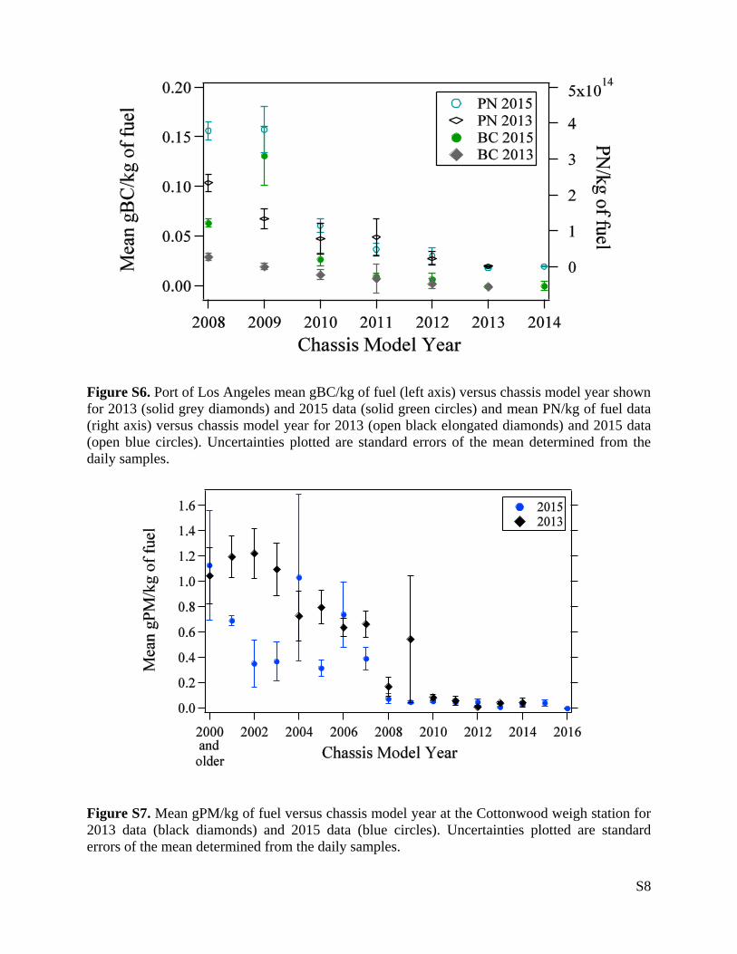
would lower from 0.18 to 0.07 gPM/kg of fuel. Fuel specific BCand PN (see Supporting Information, Figure S6) show a similarpattern with increases for the older model year vehicles.The box and whisker plot in Figure 3 shows the 2013 and
2015 gPM/kg of fuel emissions for chassis model years 2008−
2014 measured at the Port. The box denotes the 25th and 75thpercentiles for each model year and medians are represented bya horizontal line within the box. The whiskers show the 10thand 90th percentiles with measurements outside the whiskerssymbolized as diamonds (2013) and circles (2015). The meanfor each model year is represented by a filled square. Negativevalues in the data set reflect the uncertainties in determiningthe zero slope emissions, and as such also indicate an equaluncertainty in the positive direction and if omitted would biasthe means high. For the two oldest model years in Figure 3there is an obvious expansion of the interquartile range and anincrease in the number of measurements beyond the 2013 90thpercentiles. The increased means are a result of a more skewedemissions distribution. This is not due to an overalldeterioration in filter efficiency for every HDV, but an increasein the number of vehicles, originally equipped with DPFs, thathave unexplained high particle emissions. In 2013 the highestemitting 1% of the fleet was responsible for 25% of the totalgPM/kg of fuel which has increased to 53% in the 2015 dataset. 2010 model year emissions show a smaller increase in meanemissions, again as a result of more measurements at higheremission levels. 2011 and newer chassis model years show few,if any, changes over the two year period though they makeuponly 11% of the measurements in both years. The observedincreases shown here are consistent with previously reportedmeasurements at the Port of Oakland.18
In contrast, fleet turnover at Cottonwood has resulted in ayounger fleet, (0.6 years newer) responsible for approximatelyhalf of the observed reductions in fuel specific PM and BCemissions since 2013, though it did not have a significantinfluence on the fuel specific PN emissions. The 2015measurements had 25% more HDVs with chassis model year2008 and newer. Cottonwood gBC/kg of fuel emissions versuschassis model year for the 2013 (diamonds) and 2015 (circles)measurements are shown in Figure 4 with each model year
grouping shown having at least 10 measurements. Theuncertainties plotted are the SEM calculated from the dailymeans. The 2008 and newer model year vehicles show thecharacteristic drop in BC emissions due to the addition ofDPFs, with little change between the two measurement yearsfor the newer models. At Cottonwood interstate truck trafficresults in few reoccurring HDV measurements (36 out of 619unique HDVs). High emitting 2009 model year vehicles
Figure 1. Mean gPM/kg of fuel (solid bars, left axis) and mean gBC/kg of fuel (hatched bars, left-axis) and mean PN/kg of fuel (open bars,right-axis) at the Port of Los Angeles and Cottonwood locations. Both2013 (blue, left most bars) and 2015 (green, right most bars) data areshown. The uncertainties are standard errors of the mean calculatedfrom the daily means.
Figure 2. Mean gPM/kg of fuel at the Port of Los Angeles versuschassis model year for the data collected in 2013 (diamonds) and 2015(circles). The uncertainties plotted are standard errors of the meancalculated from the daily means.
Figure 3. Box and whisker plot of gPM/kg of fuel versus chassis modelyear for the 2013 (left, diamonds) and 2015 (right, circles) emissionmeasurements from the Port of Los Angeles. The box encloses the25th to the 75th percentile and the median is represented by thehorizontal line within the box. The whiskers extend from the 10th tothe 90th percentile. The black squares denote the mean and theindividual points are HDV measurements beyond the 10th and 90thpercentiles.
Figure 4. Mean gBC/kg of fuel versus chassis model year atCottonwood for 2013 (diamonds) and 2015 (circles) measurements.The uncertainties plotted are the standard errors of the meancalculated using the daily means.
observed in 2013 resulting in fuel specific BC and PM meanemissions that are higher than the 2015 mean measurementswere not repeated. A similar pattern was observed for fuelspecific PM emissions (see Supporting Information, Figure S7).A decrease in PM and BC at Cottonwood for older HDVssuggests that some vehicles in 2015 have been retrofit withDPFs in accordance with the State’s Truck and Bus rule.The State of California has a Truck and Bus Rule Reporting
System that records retrofit activity based on informationprovided by the owner. This system provided information on109 out of the 142 pre-2008 chassis model year HDVs fromCalifornia, 24 of which had reported installing retrofit DPFs.24
The mean and SEM for fuel specific PM and BC emissions ofthose 24 HDVs were 0.06 ± 0.07 and 0.03 ± 0.04, respectively,and are comparable to newer DPF-equipped HDV emissionlevels. The remaining 85 nonretrofit HDVs had mean fuelspecific PM and BC emissions of 0.66 ± 0.16 and 0.21 ± 0.001,respectively, which are an order of magnitude larger. Two ofthe 24 HDVs reported as having a retrofit DPF had PM and BCemissions at pre-DPF levels (0.84 and 0.81 gPM/kg of fuel and0.45 and 0.35 gBC/kg of fuel) indicating either the time of theinstallation was misreported or the DPF has failed or has beenuninstalled. The increase in the fraction of pre-2008 HDVsequipped with DPFs in the 2015 Cottonwood fleet accounts forthe additional PM emission reductions seen since 2013.The fuel specific particle emissions from these two locations
are significantly lower than similar measurements collected atthe Port of Oakland in 2011 and 2013.18 Directly comparablegBC/kg of fuel emissions from the Port of Los Angeles showsimilar emission trends by model year with the Port of Oaklanddata but the OHMS means are exactly an order of magnitudelower. It is important to note that there are a number ofdifferences between these two studies, different BC instrumen-tation (photoacoustic versus aethalometer), OHMS integratesemissions over 15.2 m and the Oakland study measuresemissions from a single inlet suspended off a bridge, differentfleets, and the data from the Oakland study was collected athigher operating speeds. However, despite the differences inmethod and vehicle operating modes, fuel specific NOxemissions in the two studies are similar.One possible explanation that has been explored is whether
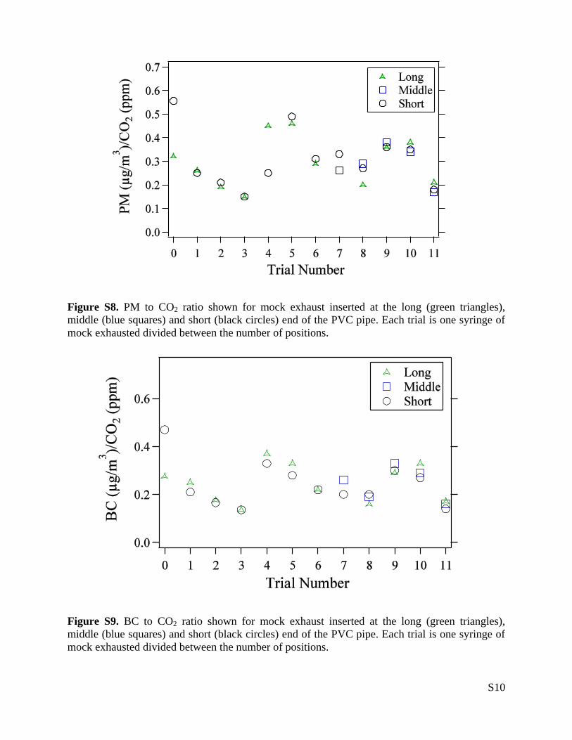
particle loss occurs in the OHMS sampling system, whichwould lead to underreporting of emissions and be consistentwith the direction of the difference. Repeatability experimentswere conducted in the lab using the OHMS sampling system,testing for particle losses in the sampling line, before and afterthe 90° bend, and before and after the exhaust fan. Throughthese experiments we have been unable to find any significantparticle losses in our sampling of PM or BC that could explain
the differences (see the Supporting Information, Figures S8−S13).The Federal particle standard for HDVs is 0.01g/bhp-h
which translates to approximately 0.07gPM/kg of fuel assumingaverage fuel consumption at our sites is 0.15 kg of fuel/bhp-h.21
In the 2015 measurements for 2008 and newer chassis modelyears 19% of the measurements at the Port and 17% of themeasurements at Cottonwood exceed 0.07 gPM/kg of fuel,indicating that a large majority of the HDVs have PM emissionslower than the certification standard. In the literature, May et al.(2014) reported chassis dynamometer results for a 2010 and2007 HDV with gPM/kg of fuel of 0.007 ± 0.004 and 0.15 ±0.14, respectively.25 Johnson et al. (2011) reported on-road PMmeasurement results for a 2008 ProStar and Volvo HDV. TheProStar never exceeded 0.01g/bhp-h while the Volvo’s PMemissions ranged as high as 0.04 (0.26 gPM/kg of fuel) butwith average emissions well below 0.01g/bhp-h.26 Quiros et al.(2016) have also recently reported on-road measurements onseven additional HDVs that were all below the PM certificationlevel.27 The literature values, though few, are more consistentwith the mean values reported here.The mean emission trends at both sites for CO, HC, NO,
NO2, and NOx are shown in the Supporting Information(Figure S14). There were no statistically significant changes inemissions of CO, NO, NO2, and NOx at the Port during theintervening two years; however, there was a statisticallysignificant increase in mean HC emissions (152%). This isthe result of methane emissions from an increase in the numberof liquefied natural gas trucks sampled during 2015 at the Port(see Table 1).17 These vehicles also increase the fleet gCO/kgof fuel means. At Cottonwood, decreasing CO emissions forthe overall fleet average corresponds to the reduction in PMemissions from older trucks. While mean fleet NOx emissionsdid not increase significantly, there was an increase for thenewer chassis model years, (see Supporting Information, FigureS14) that is currently unexplained.
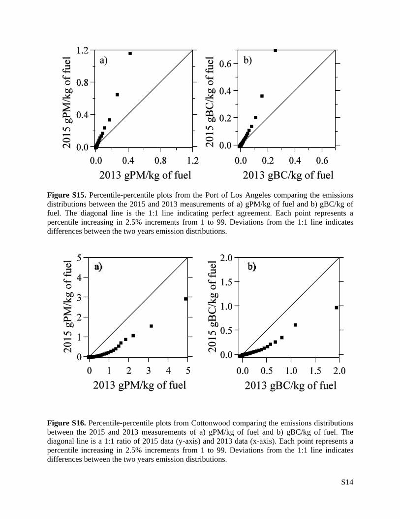
High Emitters.We have previously used a standard for highemitting HDVs as ∼0.21 gPM/kg of fuel, which isapproximately 3 times the equivalent Federal PM Certificationlimit of 0.07gPM/kg of fuel.21 The Port fleet saw increases inthe number of HDVs over 0.21 gPM/kg of fuel from 4% in2013 to over 8% in 2015, contributing to the emission increasesshown in Figures 2 and 3. Percentile−percentile plotscomparing the two years’ emissions distributions for fuelspecific PM and BC emissions at the Port of Los Angeles (seeSupporting Information, Figures S15a,b) show the 2015emission distributions deviate from the 1:1 line beginning atthe 53rd and 35th percentiles, respectively. The percentage ofHDVs over 0.21 gPM/kg of fuel at Cottonwood decreased
Table 2. 2015 Measurement Summary for a 2009 Model Year Repeat HDV at the Port of Los Angeles Showing the Date, Beforeor After Noon, Fuel Specific Emissions, Speed and Acceleration, IR Exhaust temperatures (°C), Roadside Opacity Percentage,and Pass or Fail of the Roadside Test
from 49% in 2013 to 23% in 2015 as a result of fleet-turnoverand retro-fit activities. Percentile−percentile plots (FiguresS16a,b) show the large negative percentile changes atCottonwood for PM and BC fuel specific emissions.With the observed increases in fuel specific PM and BC
emissions at the Port, particularly in the oldest model years,there is also an increase in the variability of the repeatmeasurements, both within the 2015 measurements andreoccurring trucks measured in both years. In general theemission’s variability increases with increasing mean emissions(see Supporting Information, Figure S17), a pattern that hasbeen previously observed for gaseous emissions from light-dutyvehicles.28
One 2009 vehicle at the Port of Los Angeles was measuredsix times during the 2015 campaign and exhibits an apparenttime dependence in its particle emissions. Table 2 summarizesthe six emission measurements collected over the course of 4days in chronological order with measurements made beforenoon (AM, bold-italic font) differentiated from those collectedafter noon (PM). Exit accelerations were invalid for allmeasurements due to an equipment problem; all othermeasurements that exceeded confidence limits are denoted bya dash in Table 2. Noticeably the DPF in this HDV is not inperfect working order, as most of the gPM/kg of fuel emissionsare significantly higher than the average for any model year atthe Port and often resemble pre-DPF HDV emission levels.21
However, the two morning measurements on March 26th and27th (2.0 and 0.14 gPM/kg of fuel) were much lower, and themeasurement on the morning of the 27th is close to the Port’sfleet mean of 0.11 ± 0.01.Concurrent with OHMS measurements the State of
California conducted random roadside opacity inspectionsusing a snap-acceleration test which reports an average tailpipeopacity reading for three rapid acceleration events.29,30 The2009 HDV discussed in Table 2 was tested by the inspectionteam on the afternoon of the 26th and the morning of the 27thimmediately after passing through the OHMS tent. Theinspection results mirror the OHMS results with the vehiclehaving an afternoon average tailpipe opacity of 95.5% andfailing the test followed the next morning with a passing opacitytest of only 10.8%. If repairs were attempted on the vehicleovernight they were not lasting as we measured the vehicle onthe afternoon of the 27th with results that would again farexceed limits.The extreme variability of the particle emissions from this
vehicle, observed by two different testing methods, is difficult toexplain. One possibility is that this truck’s DPF has beentampered with or removed leaving tailpipe particle emissionsstrictly a function of engine operation. However, the observedentrance and exit speeds for these measurements are all similar,as well as the State’s opacity inspection. Fuel specific COemissions correlate with the fuel specific PM and BC emissionsindicating fuel enrichment for the high PM events. Figure 5shows FMPS fuel specific particle size distribution datacollected in the morning (solid line) and afternoon (dashedline) of March 26th for this HDV post-processed with TSI’ssoot inversion matrix. PM increases in the afternoon result in ashift in the peak particle size from ∼70 nm to >150 nm. Thisshift in peak particle size is also seen between the morning andafternoon measurements, collected on March 27th, as well as anumber of other high emitting HDVs at the Port of LosAngeles in 2015. The shift in the particle distribution isconsistent with the use of large amounts of exhaust gas
recirculation (EGR) in combustion, which would lower NOxemissions by enrichening the cylinder air to fuel ratio, and hasbeen observed by other researchers.31,32 Increased EGR in theafternoon could be a consequence of increased ambienttemperature and/or may reflect this vehicles particular workcycle.A second potential explanation has to include the possibility
that the DPF remains in the vehicle but only functionssporatically. It has been shown that cracks due to thermalexpansion or vibrations over time will reduce filter surface areain a DPF, as well as cause filter “leakages” which may increaseas the day progresses.33,34 In addition, the presence of a soot-cake significantly increases the filter efficiency of the DPF, thusit is also within the realm of possibilities that some of theemissions variability is related to its regeneration frequencywith lower PM emissions prior to a regeneration event.35
To date there has been no research that has looked at howand why DPFs fail and the resultant emissions reductions thatare lost. The Port measurements show the largest increase inemissions are from the 2008−2010 model year vehicles whichwere initially designed with higher engine out PM emissions, tolimit NOx emissions since they do not have a NOxaftertreatment system.13 DPFs in these vehicles therfore willrequire more frequent active regeneration events, where fuel isintroduced into the filter to combust the accumulated soot andrestore exhaust flow rates. The increased thermal stress coupledwith the likely need to manually remove accumulated ash moreoften may increase the chances for defects to be introducedinto these early generation filters. Many of these issues havebeen addressed in the later model vehicles (2011 and newer) asengines are now designed to limit PM emissions reducing thedemand on DPFs. However, ensuring the long-term integrity ofinstalled DPFs is paramount to maintaining the particleemissions reductions achieved to date.
■ ASSOCIATED CONTENT*S Supporting InformationThe Supporting Information is available free of charge on theACS Publications website at DOI: 10.1021/acs.est.6b06172.
Example of how particle number per kilogram of fuel wascalculated; estimation of standard errors of the mean forreported uncertainties; field emissivity calibration of theinfrared camera; tests of PVC pipe particle loss;additional figures (PDF)
Figure 5. Fuel specific particle size distributions collected with a FastMobility Particle Sizer using the soot inversion on March 26th beforenoon (AM, solid line) and afternoon (PM, dashed line) from a 2009HDV at the Port of Los Angeles in 2015.
Corresponding Author*Phone: (303) 871-2584; e-mail: [email protected]; address:Department of Chemistry and Biochemistry, University ofDenver, Denver, Colorado 80208
ORCID
Molly J. Haugen: 0000-0003-2394-7603Gary A. Bishop: 0000-0003-0136-997XNotesThe authors declare the following competing financialinterest(s): G. A. Bishop acknowledges receipt of patentroyalty payments from Envirotest, an operating subsidiary ofOpus Inspection, which licenses vehicle emissions testingtechnology developed at the University of Denver.
■ ACKNOWLEDGMENTS
The authors would like to thank the California EnvironmentalProtection Agency-Air Resources Board for funding (ContractNo. 11-309), the California Highway Patrol and Trans PacificContainer Service Corporation for site access, the University ofDenver, TSI Inc for software, and Ian Stedman for logisticalsupport. We acknowledge the late Donald Stedman for theinvention of the OHMS and his irreplaceable guidance.
■ REFERENCES(1) Health Risk Assessment for Diesel Exhaust, Part B; Office ofEnvironmental Health Hazard Assessment, California EnvironmentalProtection Agency: Sacramento CA, 1998.(2) Risk Reduction Plan to Reduce Particulate Matter Emissions fromDiesel-fueled Engines and Vehicles; California Air Resources Board,Sacramento, CA, 2000.(3) International Agency for Research on Cancer IARC: Dieselengine exhaust carcinogenic. Press Release 213. http://www.iarc.fr/en/media-centre/pr/2012/pdfs/pr213_E.pdf (accessed August 2016).(4) Traffic-Related Air Pollution: A Critical Review of the Literature onEmissions, Exposure, and Health Effects. A Special Report of the HEIPanel of the Health Effects of Traffic-related Air Pollution; Health EffectsInstitute, 2010.(5) Simon, H.; Reff, A.; Wells, B.; Xing, J.; Frank, N. Ozone trendsacross the United States over a period of decreasing NOx and VOCemissions. Environ. Sci. Technol. 2015, 49, 186−195.(6) Bahadur, R.; Feng, Y.; Russell, L. M.; Ramanathan, V. Impact ofCalifornia’s air pollution laws on black carbon and their implicationsfor direct radiative forcing. Atmos. Environ. 2011, 45, 1162−1167.(7) Gentner, D. R.; Jathar, S. H.; Gordon, T. D.; Bahreini, R.; Day, D.A.; El Haddad, I.; Hayes, P. L.; Pieber, S. M.; Platt, S. M.; de Gouw, J.;Goldstein, A. H.; Harley, R. A.; Jimenez, J. L.; Prevot, A. S. H.;Robinson, A. L. Review of urban secondary organic aerosol formationfrom gasoline and diesel motor vehicle emissions. Environ. Sci. Technol.2017, 51 (3), 1074−1093.(8) The Clean Air Act; U.S. Environmental Protection Agency, 2004.(9) Emission standards and supplemental requirements for 2007 andlater model year diesel heavy-duty engines and vehicles. Code ofFederal Regulations, Title 40, Chapter I, Subchapter C, Part 86, SubpartA, Section 86.007-11 2008.(10) Regulation to reduce emissions of diesel particulate matter,oxides of nitrogen and other criteria pollutants, from in-use heavy-dutydiesel-fueled vehicles. California Code of Regulations, Title 13, Division3, Chapter 1, 2008.(11) Amendments to the regulation to reduce emissions of dieselparticulate matter, oxides of nitrogen and other criteria pollutants fromin-use on-road diesel-fueled vehicles. California Code of Regulations,Title 13, 2011.
(12) Advanced Collaborative Emissions Study (ACES). LifetimeCancer and Non-Cancer Assessment in Rats Exposed to New-TechnologyDiesel Exhaust; Health Effects Institute: Boston, MA, 2015.(13) Bell, J. Modern Diesel Technology: Electricity and Electronics, 2nded.; Cengage Learning, 2013.(14) Misra, C.; Collins, J. F.; Herner, J. D.; Sax, T.; Krishnamurthy,M.; Sobieralski, W.; Burntizki, M.; Chernich, D. In-use NOx emissionsfrom model year 2010 and 2011 heavy-duty diesel engines equippedwith aftertreatment devices. Environ. Sci. Technol. 2013, 47 (14),7892−7898.(15) Port of Long Beach; Port of Los Angeles San Pedro Bay PortsClean Air Action Plan: About the Clean Air Action Plan. http://www.cleanairactionplan.org (accessed Dec. 2016).(16) 2010 Update San Pedro Bay Ports Clean Air Action Plan; ThePort of Los Angeles; Port of Long Beach, 2010.(17) Bishop, G. A.; Schuchmann, B. G.; Stedman, D. H.; Lawson, D.R. Emission changes resulting from the San Pedro Bay, CaliforniaPorts Truck Retirement Program. Environ. Sci. Technol. 2012, 46, 551−558.(18) Preble, C. V.; Dallmann, T. R.; Kreisberg, N. M.; Hering, S. V.;Harley, R. A.; Kirchstetter, T. W. Effects of particle filters and selectivecatalytic reduction on heavy-duty diesel drayage truck emissions at thePort of Oakland. Environ. Sci. Technol. 2015, 49 (14), 8864−8871.(19) Herner, J. D.; Hu, S.; Robertson, W. H.; Huai, T.; Collins, J. F.;Dwyer, H.; Ayala, A. Effect of advanced aftertreatment for PM andNOx control on heavy-duty diesel truck emissions. Environ. Sci.Technol. 2009, 43, 5928−5933.(20) Kozawa, K. H.; Park, S. S.; Mara, S. L.; Herner, J. D. Verifyingemission reductions from heavy-duty diesel trucks operating onSouthern California freeways. Environ. Sci. Technol. 2014, 48 (3),1475−1483.(21) Bishop, G. A.; Hottor-Raguindin, R.; Stedman, D. H.;McClintock, P.; Theobald, E.; Johnson, J. D.; Lee, D.-W.; Zietsman,J.; Misra, C. On-road heavy-duty vehicle emissions monitoring system.Environ. Sci. Technol. 2015, 49 (3), 1639−1645.(22) Bishop, G. A.; Schuchmann, B. G.; Stedman, D. H. Heavy-dutytruck emissions in the South Coast Air Basin of California. Environ. Sci.Technol. 2013, 47 (16), 9523−9529.(23) Dallmann, T. R.; Harley, R. A.; Kirchstetter, T. W. Effects ofdiesel particle filter retrofits and accelerated fleet turnover on drayagetruck emissions at the Port of Oakland. Environ. Sci. Technol. 2011, 45,10773−10779.(24) California Environmental Protection Agency Air ResourcesBoard Truck and Bus Regulation Reporting. http://www.arb.ca.gov/msprog/onrdiesel/reportinginfo.htm (accessed July 2016).(25) May, A. A.; Nguyen, N. T.; Presto, A. A.; Gordon, T. D.; Lipsky,E. M.; Karve, M.; Gutierrez, A.; Robertson, W. H.; Zhang, M.;Brandow, C.; et al. Gas- and particle-phase primary emissions from in-use, on-road gasoline and diesel vehicles. Atmos. Environ. 2014, 88,247−260.(26) Johnson, K. C.; Durbin, T. D.; Jung, H.; Cocker, D. R.; Bishnu,D.; Giannelli, R. Quantifying in-use PM measurements for heavy dutydiesel vehicles. Environ. Sci. Technol. 2011, 45 (14), 6073−6079.(27) Quiros, D. C.; Thiruvengadam, A.; Pradhan, S.; Besch, M.;Thiruvengadam, P.; Dermirgok, B.; Carder, D.; Oshinuga, A.; Huai, T.;Hu, S. Real-world emissions from modern heavy-duty diesel, naturalgas, and hybrid diesel trucks operating along major California freightcorridors. Emiss. Control Sci. Technol. 2016, 2, 156−172.(28) Bishop, G. A.; Stedman, D. H.; Ashbaugh, L. Motor vehicleemissions variability. J. Air Waste Manage. Assoc. 1996, 46, 667−675.(29) Snap Acceleration Smoke Test Procedure for Heavy-Duty PoweredVehicles; Society of Automotive Engineers, Inc., 1996.(30) California Air Resources Board. Heavy-Duty Diesel InformationSeries. https://www.arb.ca.gov/enf/hdvip/hdvip_pamphlet.pdf (ac-cessed February 2017).(31) Li, X.; Xu, Z.; Guan, C.; Huang, Z. Particle size distributions andOC, EC emissions from a diesel engine with the application of in-cylinder emission control strategies. Fuel 2014, 121, 20−26.