62
Thermal Imaging Diagnostic Development: Ratio Pyrometry Arun Nair Graduate Student Mechanical and Aerospace Engineering

Thermal Imaging Diagnostic Development:
Ratio Pyrometry
Arun NairGraduate Student
Mechanical and Aerospace Engineering
Overview• Measurement of temperature
– Contact methods• Thermometers• Thermocouples
– Non contact methods (Pyrometry)• Infrared thermometers• Pyrometry of gases/flames
– Thin filament pyrometry– Soot pyrometry– Ratio pyrometry

Overview• Thin filament pyrometry
– Placing a thin filament in flame. – Radiative emissions from the filament correlated with
flame temperature. – Typically Silicon carbide (SiC) is used as filament
• Soot pyrometry– Soot (carbon) particles in flames– Emissions from soot correlated with flame temperature
• Ratio pyrometry

Ratio pyrometry• Intensity ratio approach
– Ratio of intensity at two different wavelengths calculated
– Ratio correlated to flame temperature
• Wien's law
h: Planck’s constant c: Speed of light
k: Boltzmann’s constant T: Temperature
𝐼𝑏(λ, ): 𝑇 Radiance of blackbody : Wavelength
Ratio pyrometry• Intensity ratio
• Temperature
• Color ratio approach– Ratio of two different colors calculated– Ratio correlated to flame temperature
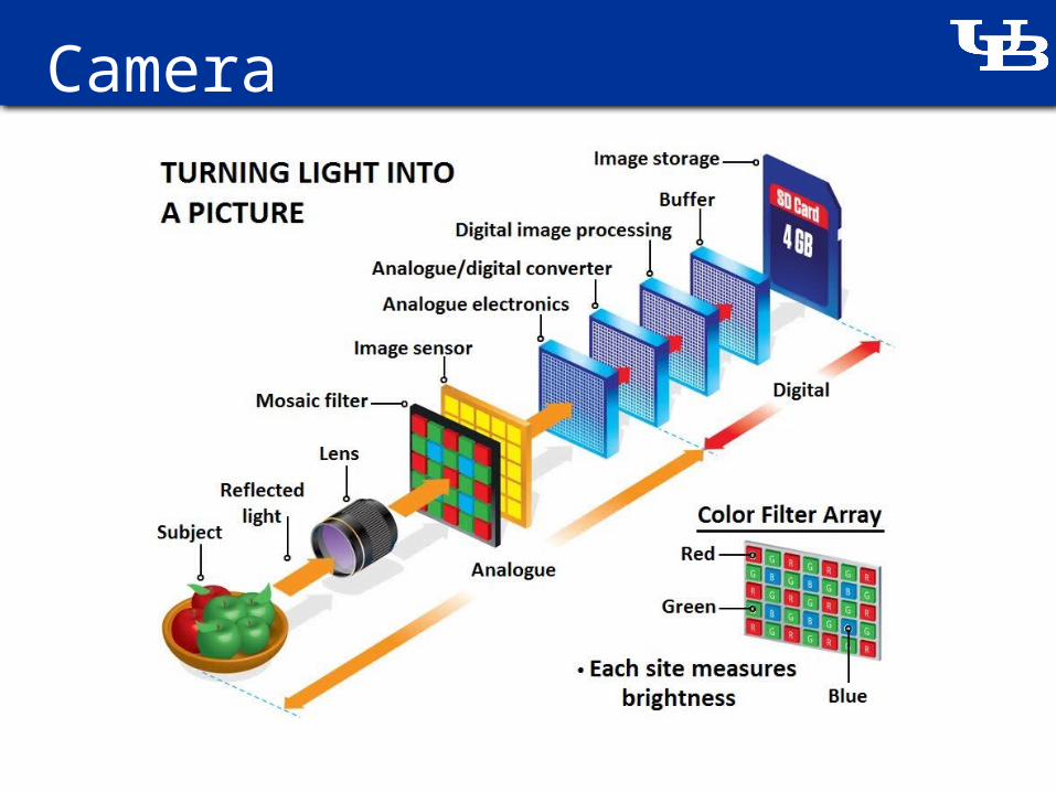
Camera

Image
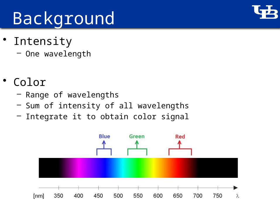
Background• Intensity
– One wavelength
• Color– Range of wavelengths– Sum of intensity of all wavelengths– Integrate it to obtain color signal

Background• Objects when heated:
– Melt, boil– Burn– Glow
• Emit light when the burn and/or glow
• Planck’s law

Background• Color ratio approach
h: Planck’s constant ε: Emissivity
k: Boltzmann’s constant T: Temperature
c: Speed of light. Λ: Wavelength
𝐼𝑏 (λ, ): 𝑇 Radiance of blackbody η: Filter efficiency
Grey body assumption: Emissivity is a constant.

Ratio pyrometry • Present research
– Combine thin filament pyrometry with ratio pyrometry• (Peter Kuhn et. al. , Bin Ma et. al.)
• Advantages– Independent of emissivity– Field measurement of temperature instead of line(TFP) or point
(conventional methods)– Low cost method for pyrometry– Works for any commercially available digital camera
• Potential– Data can be extracted from archived video footage/images

Goal• Determine temperature field of body from a picture
• Is it possible?– Yes
• Commercial cameras available– Expensive: $30,000 +– Tailored for low
temperatures

Study• Calculate the signal values• Planck’s law
• Integral function in Matlab– int(function, variable, lower limit, upper limit)
• Numerical integration– Composite Simpson’s rule
• Blackbody radiation function– Fraction of radiation emitted up to a particular wavelength
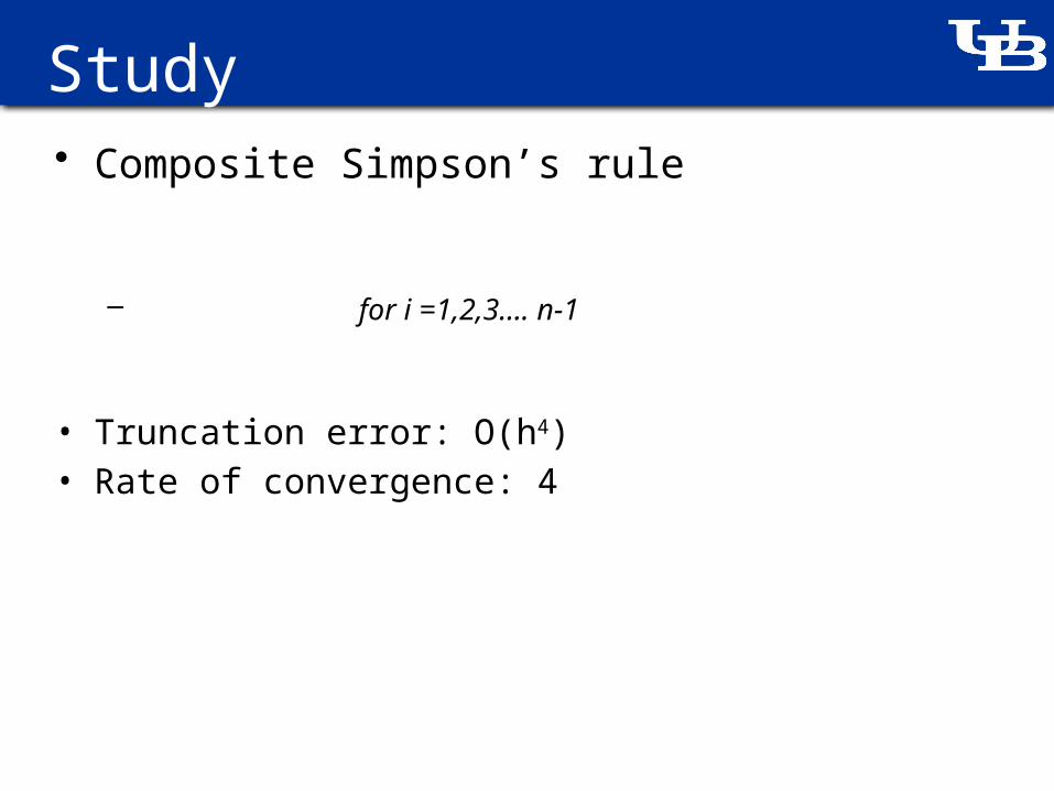
Study• Composite Simpson’s rule
– for i =1,2,3…. n-1
• Truncation error: O(h4)• Rate of convergence: 4

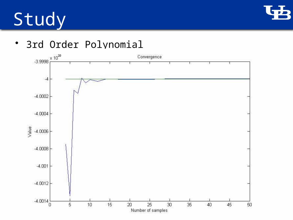
Study• Convergence
• Slope: -4.000104313216625

Study• Blackbody radiation function

Study
• Blackbody radiation function – Thermal Radiation Heat Transfer (Second Edition)
• Robert Siegel & John R. Howell
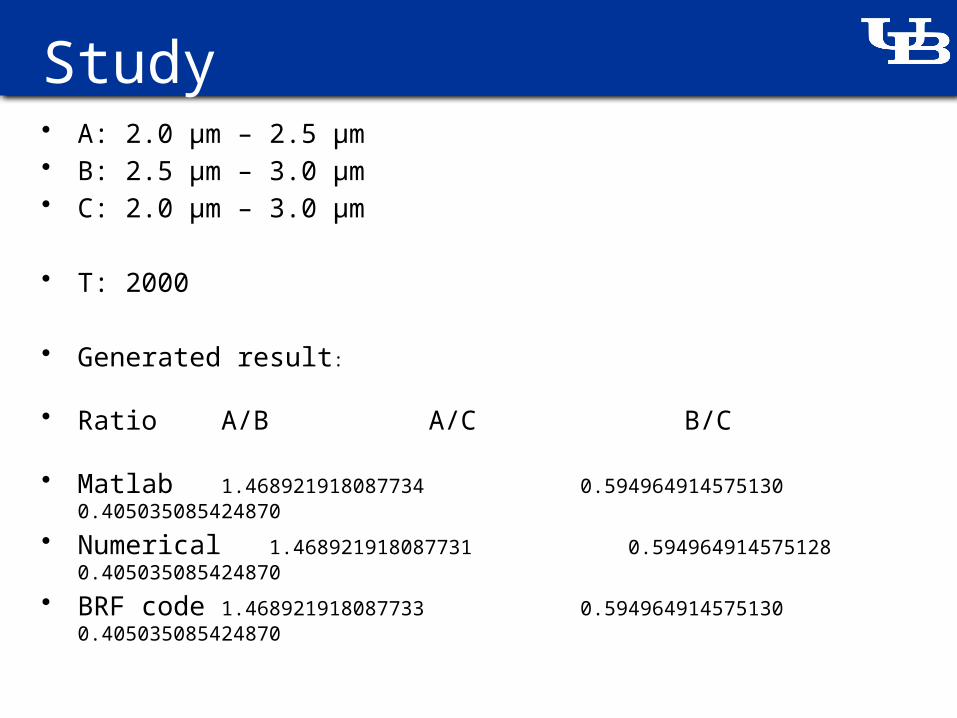
Study• A: 2.0 μm – 2.5 μm • B: 2.5 μm – 3.0 μm • C: 2.0 μm – 3.0 μm
• T: 2000
• Generated result:
• Ratio A/B A/C B/C
• Matlab 1.468921918087734 0.594964914575130 0.405035085424870
• Numerical 1.468921918087731 0.594964914575128 0.405035085424870
• BRF code 1.468921918087733 0.594964914575130 0.405035085424870

Study• Filter efficiency: η(λ)
• Nikon D70– Kuhn et. al.
• Data digitized using
software
• Blue: 3.70nm – 5.6nm • Green: 3.70 nm – 6.2nm
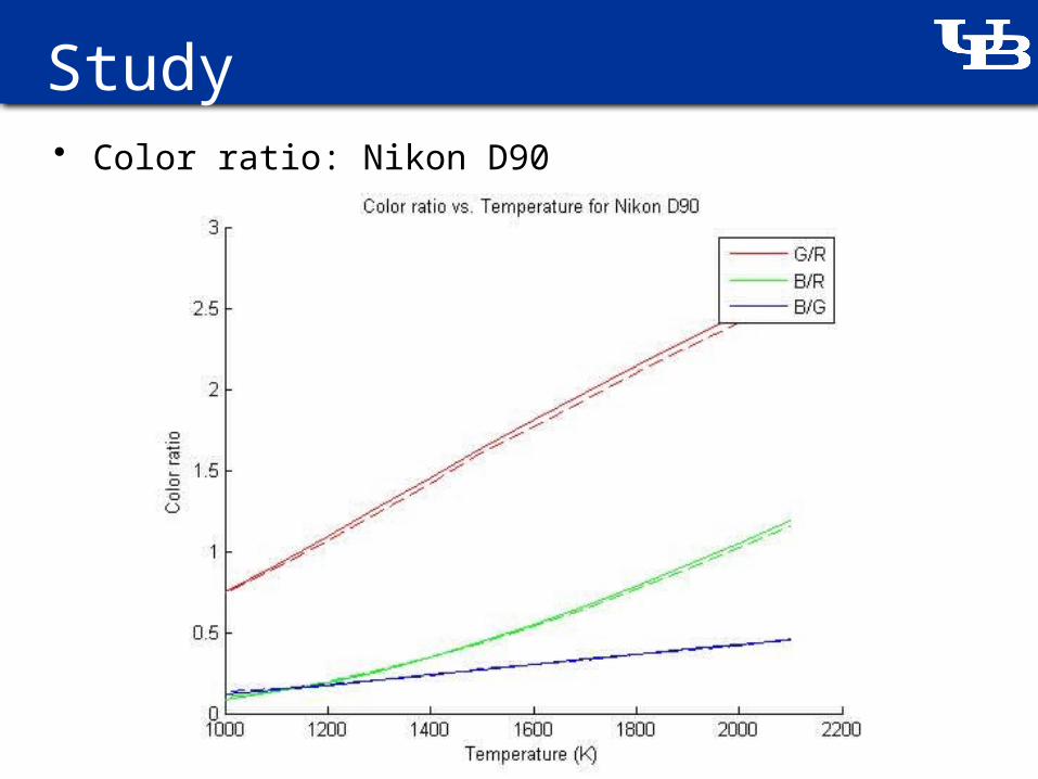
Study• Color ratio: Nikon D90

Study• Filter efficiency: η(λ)
– Experimental method:• Spectrum from known source is dispersed using a diffraction
grating• The spectrum is imaged using a camera and the component
colors separated• Spectrum is calibrated and normalized using spectral lines
from mercury vapor lamp.– 404.7 nm, 435.8 nm, 546.1 nm, 578.2 nm
– Analytical method:• Develop a “black box” function, which correlates input signal
to output temperature

Study• Filter efficiency: η(λ)
– Ideally Gaussian distribution
– Functions considered:• Polynomial function
• Cubic spline function
• Quadratic spline function

Study• Method of Least Squares
N-order polynomial
Study• Method of Least Squares
M temperature samples

Study• Method of Least Squares
j=0 to N
n x n matrix
n x 1 matrix
n x 1 matrix

Study• 3rd Order Polynomial
3.50E-07 4.00E-07 4.50E-07 5.00E-07 5.50E-07 6.00E-070
0.2
0.4
0.6
0.8
1
1.2
f(x) = − 4.00523163511332E+020 x³ + 541022875015011 x² − 236180096.469051 x + 33.5692180090286
Green Channel
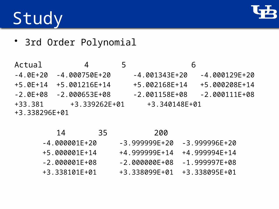
Study• 3rd Order Polynomial
Actual 4 5 6-4.0E+20 -4.000750E+20 -4.001343E+20 -4.000129E+20
+5.0E+14 +5.001216E+14 +5.002168E+14 +5.000208E+14
-2.0E+08 -2.000653E+08 -2.001158E+08 -2.000111E+08
+33.381 +3.339262E+01 +3.340148E+01 +3.338296E+01
14 35 200-4.000001E+20 -3.999999E+20 -3.999996E+20
+5.000001E+14 +4.999999E+14 +4.999994E+14
-2.000001E+08 -2.000000E+08 -1.999997E+08
+3.338101E+01 +3.338099E+01 +3.338095E+01
Study• 3rd Order Polynomial
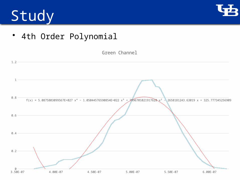
Study• 4th Order Polynomial
3.50E-07 4.00E-07 4.50E-07 5.00E-07 5.50E-07 6.00E-070
0.2
0.4
0.6
0.8
1
1.2
f(x) = 5.0875803099567E+027 x⁴ − 1.05044576590854E+022 x³ + 7996701021917631 x² − 2658181243.63019 x + 325.777345256909
Green Channel

Study• 4th Order Polynomial
Actual 12 14 16+5.0E+27 +5.087979E+27 +5.128295E+27 +5.118779E+27
-1.0E+22 -1.018115E+22 -1.026373E+22 -1.024293E+22
+8.0E+15 +8.138792E+15 +8.201706E+15 +8.184809E+15
-3.0E+09 -3.046873E+09 -3.067996E+09 -3.061950E+09
+325.78 +3.316646E+02 +3.343004E+02 +3.334974E+02
50 100 500+5.023995E+27 +4.834364E+27 +5.434768E+27
-1.004838E+22 -9.667522E+21 -1.086809E+22
+8.036259E+15 +7.751986E+15 +8.644015E+15
-3.011967E+09 -2.918543E+09 -3.210330E+09
+3.272469E+02 +3.158439E+02 +3.512897E+02

Study• 4th Order Polynomial

Study• 5th Order Polynomial
3.50E-07 4.00E-07 4.50E-07 5.00E-07 5.50E-07 6.00E-070
0.2
0.4
0.6
0.8
1
1.2
f(x) = 7.79393189172729E+034 x⁵ − 1.88396778902105E+029 x⁴ + 1.80250813001394E+023 x³ − 8.53482157102074E+016 x² + 20011050584.8252 x − 1859.83317642822
Green Channel

Study• 5th Order Polynomial

Study• Signal Ratio
3.50E-07 4.00E-07 4.50E-07 5.00E-07 5.50E-07 6.00E-070
0.2
0.4
0.6
0.8
1
1.2
f(x) = − 4.00523163511332E+020 x³ + 541022875015011 x² − 236180096.469051 x + 33.5692180090286
Green Channel
Wavelength (m)
Sen
sitiv
ity

Study• Signal Ratio
3.50E-07 4.00E-07 4.50E-07 5.00E-07 5.50E-070
0.2
0.4
0.6
0.8
1
1.2
f(x) = 6.24807341207282E+020 x³ − 989260610456236 x² + 509762744.770074 x − 85.1750066574398
Blue Channel
Wavelength (m)
Sen
sitiv
ity

Study• Signal Ratio
– 2nd Order Polynomial
Actual 10 15-1.180233E+14 -1.182471E+14 -1.180380E+14
+1.081001E+08 +1.082962E+08 +1.081126E+08
-23.96354 -2.395876E+01 -2.396334E+01
-5.623263E+13 -5.632741E+13 -5.623903E+13
+5.691230E+07 +5.700364E+07 +5.691833E+07
-13.73959 -1.373959E+01 -1.373959E+01
20 30-1.180269E+14 -1.180233E+14
+1.081031E+08 +1.081001E+08
-2.396351E+01 -2.396354E+01
-5.623422E+13 -5.623261E+13
+5.691377E+07 +5.691228E+07
-1.373959E+01 -1.373959E+01

Study• Signal Ratio
– 3rd Order Polynomial
Actual 50 200 500+5.882149E+20 +7.032672E+20 +5.905079E+20 +5.612230E+20
-9.368183E+14 -1.113896E+15 -9.403226E+14 -8.962225E+14
+4.848695E+8 +5.733508E+08 +4.866119E+08 +4.649229E+08
-81.26233 -9.552129E+01 -8.154242E+01 -7.807783E+01
-3.991030E+20 -4.243452E+20 -3.995615E+20 -3.947716E+20
+5.388299E+14 +5.636853E+14 +5.392815E+14 +5.345657E+14
-2.350623E+8 -2.408562E+08 -2.351677E+08 -2.340656E+08
+33.38127 +3.338127E+01 +3.338127E+01 +3.338127E+01
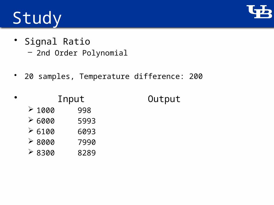
Study• Signal Ratio
– 2nd Order Polynomial
• 20 samples, Temperature difference: 200
• Input Output 1000 998 6000 5993 6100 6093 8000 7990 8300 8289

Study• Signal Ratio
– 3rd Order Polynomial
• 200 samples, Temperature difference: 200
• Input Output 6010 6009 8268 8267 10479 10529 21637 21628

Study• Signal Ratio
– 3rd Order Polynomial
• 500 samples, Temperature difference: 5
• Input Output 3463 3463 5924 5921 6081 6078 8237 8221 9003 8980 11257 11201

Study• Cubic spline
• Piecewise continuous polynomials
• Given n data points (x1 ,y1) , (x2 ,y2) …(xn ,yn)
y1 = a1x13+ b1x1
2 + c1x1+ d1
yn = anxn3+ bnxn
2 + cnxn+ dn
• C1 continuity: • Slopes are equal at internal points
3aixi+12+ 2bixi+1+ ci = 3ai+1xi+1
2+ 2bi+1xi+1+ ci+1
• Slopes are 0 at endpoints
3aixi2 + 2bixi + ci = 0
• C2 continuity: Second derivative is zero
6aixi + 2bi= 0

Study• Cubic spline
• C0 continuity:
ai λi+13+ bi λi+1
2+ ci λi+1+ di = ai+1 λi+13+ bi+1 λi+1
2+ ci+1 λi+1+ di+1
• C1 continuity: • Slopes are equal at internal points
3ai λi+12 + 2bi λi+1 + ci = 3ai+1 λi+1
2 + 2bi+1 λi+1 + ci+1
• Slopes are 0 at endpoints
3ai λi2 + 2bi λi + ci = 0
• C2 continuity: Second derivative is zero at internal points
6ai λi+1+ 2bi= 6ai+1 λi+1+ 2bi+1
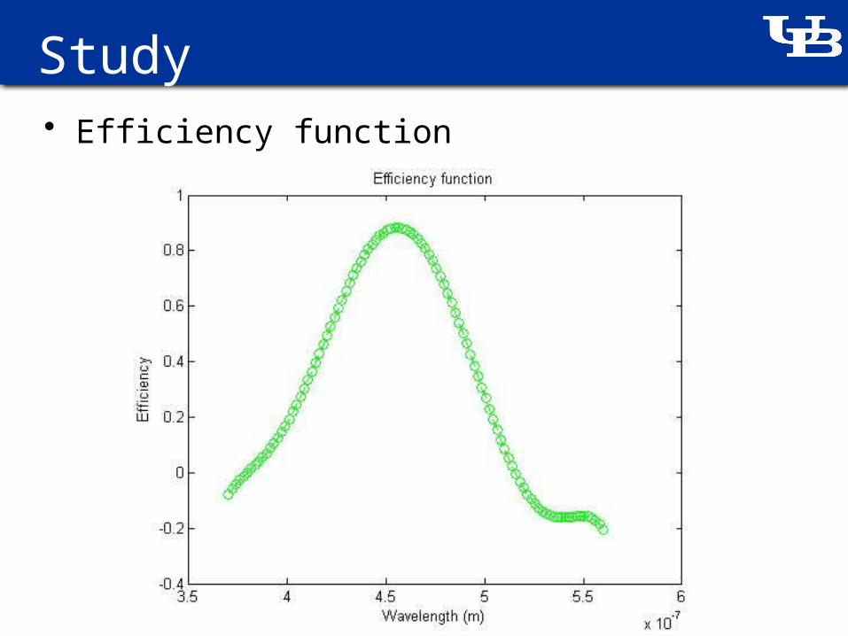
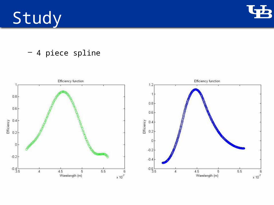
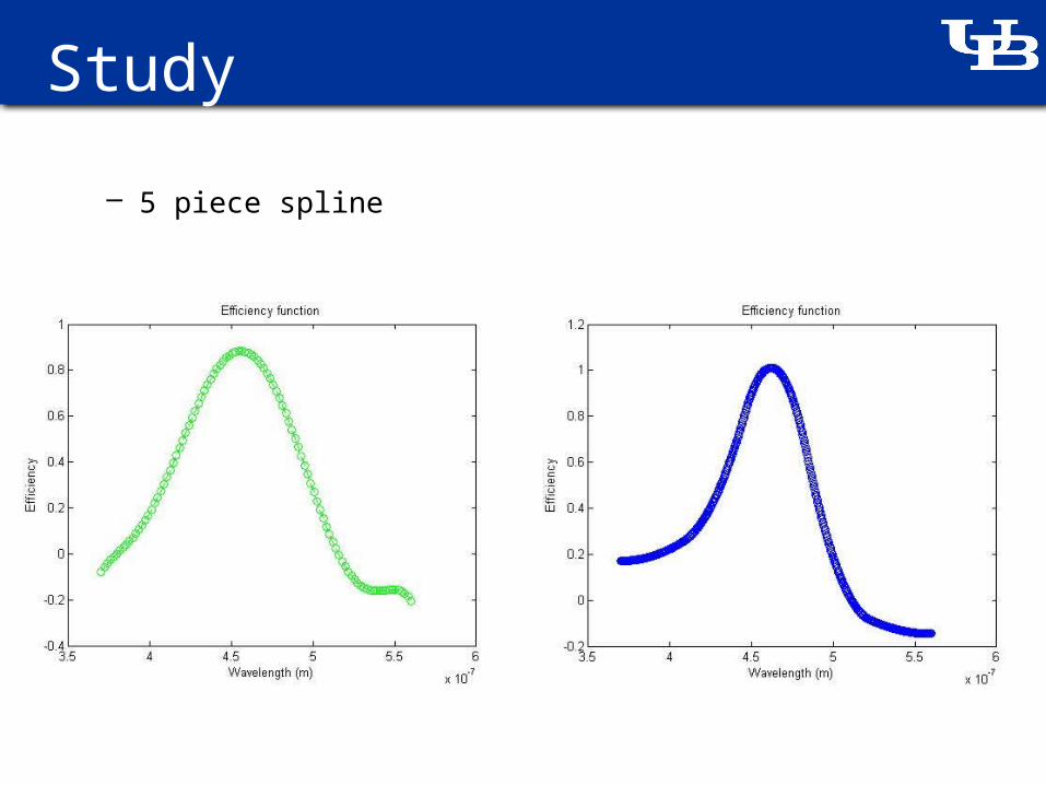
Study• Efficiency function

Study• Efficiency function
– Cubic Spline: 4 points (3 piece spline)
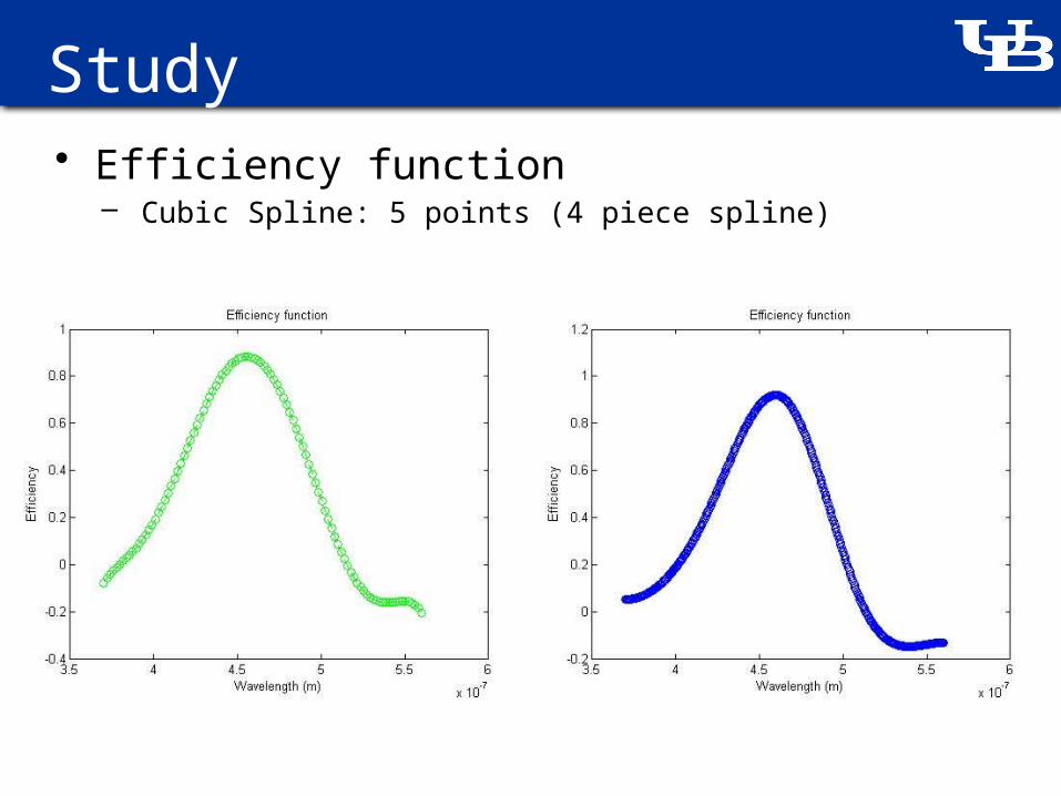
Study• Efficiency function
– Cubic Spline: 5 points (4 piece spline)

Study• Efficiency function
– Cubic Spline: 6 points (5 piece spline)
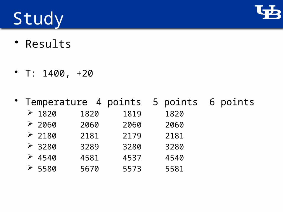
Study• Results
• T: 1400, +20
• Temperature 4 points 5 points 6 points 1820 1820 1819 1820 2060 2060 2060 2060 2180 2181 2179 2181 3280 3289 3280 3280 4540 4581 4537 4540 5580 5670 5573 5581

Study• Signal Ratio
Blue filter Green filter

Study• Cubic spline: 3 piece
Blue filter Green filter

Study• Cubic spline: 4 piece
Blue filter Green filter

Study• Cubic spline: 5 piece
Blue filter Green filter
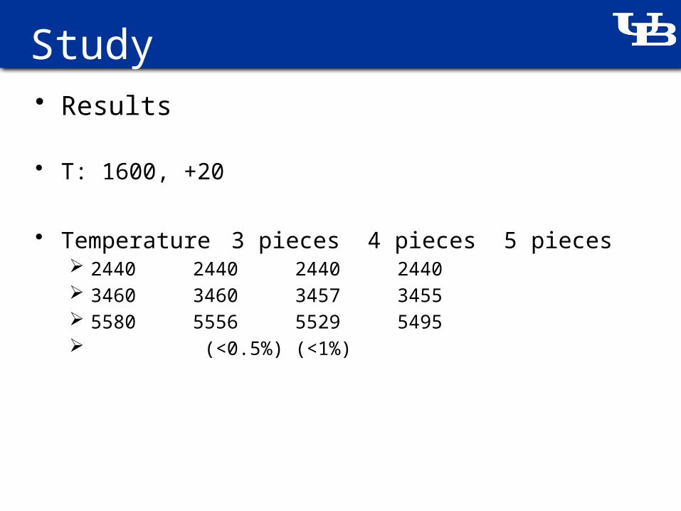
Study• Results
• T: 1600, +20
• Temperature 3 pieces 4 pieces 5 pieces 2440 2440 2440 2440 3460 3460 3457 3455 5580 5556 5529 5495 (<0.5%) (<1%)

Study• Quadratic spline
• C0 continuity:
ai λi+13+ bi λi+1
2+ ci = ai+1 λi+13+ bi+1 λi+1
2+ ci+1
• C1 continuity: • Slopes are equal at internal points
2ai λi+1 + bi = + 2ai+1 λi+1 + bi+1
• Slopes are 0 at endpoints
2ai λi + bi = 0
Study
– 4 piece spline
Study
– 5 piece spline

Study• Results
• T: 1400, +20
• Temperature 5 pieces 1960 1959 2220 2219 2780 2779 3580 3577

Study• Quadratic spline: 3 piece
Blue filter Green filter
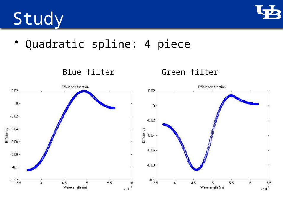
Study• Quadratic spline: 4 piece
Blue filter Green filter

Study• Quadratic spline: 5 piece
Blue filter Green filter
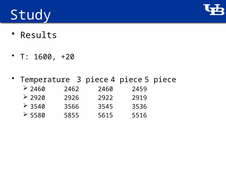
Study• Results
• T: 1600, +20
• Temperature 3 piece 4 piece 5 piece 2460 2462 2460 2459 2920 2926 2922 2919 3540 3566 3545 3536 5580 5855 5615 5516
Summary
• Develop ratio pyrometry technique for digital camera– Calculate temperature from images
• Advantages– Independent of emissivity– Field measurement of – Low cost method– Works for any commercially available digital camera– Potential to obtain experimental data from digital image/footage
• Study– Develop codes for calculating signal
• Matlab integration, Numeric integration, Blackbody radiation function

Summary• Study
– Black box function to convert signal to temperature• Polynomial functions• Cubic splines• Quadratic splines
– Code developed to calculate signal and signal ratio• 3rd order polynomial with 20 samples• 4th order polynomial with approximately 50 samples• Signal ratio of 3rd order polynomials with 500 samples
– Too many samples required – Cubic splines
• High level of accuracy for signal with 6 points• Signal ratio decreasing in accuracy with more samples
– Quadratic splines• Better results


