89
a survey of spatial economic planning models in the netherlands NAi Publishers A survey of spatial economic planning models in the Netherlands Theory, application and evaluation

1 a s u rv e y o f s pat i a l eco n om i c p l a nni n g mo d el s i n t he ne t her l a nd s
NAi Publishers
A survey of spatial economic planning models in the Netherlands
Theory, application and evaluation

a surve y of spatial economic pl anning model s in the nether l ands . theory, applic ation and e valuation
Frank van OortMark ThissenLeo van Wissen(eds.)
NAi Publishers, RotterdamNetherlands Institute for Spatial Research (rpb), Den Haag2005
Earlier publications
Een andere marktwerking
Barrie Needham (2005)
isbn 90 5662 437 7
Kennis op de kaart. Ruimtelijke patronen in de kenniseconomie
Raspe et al. (2004)
isbn 90 5662 414 8
Scenario’s in Kaart. Model- en ontwerpbenaderingen voor
toekomstig ruimtegebruik
Groen et al. (2004)
isbn 90 5662 377 X
Unseen Europe. A survey of EU politics and its impact on spatial
development in the Netherlands, Van Ravesteyn & Evers
(2004)
isbn 90 5662 376 1
Behalve de dagelijkse files. Over betrouwbaarheid van reistijd
Hilbers et al. (2004)
isbn 90 5662 375 3
Ex ante toets Nota Ruimte
cpb, rpb, scp (2004)
isbn 90 5662 412 1
Tussenland
Frijters et al. (2004)
ISBN 90 5662 373 7
Ontwikkelingsplanologie. Lessen uit en voor de praktijk
Dammers et al. (2004)
isbn 90 5662 374 5
Duizend dingen op een dag. Een tijdsbeeld uitgedrukt in ruimte
Galle et al. (2004)
isbn 90 5662 372 9
De ongekende ruimte verkend
Gordijn (2003)
isbn 90 5662 336 2
De ruimtelijke effecten van ict
Van Oort et al. (2003)
isbn 90 5662 342 7
Landelijk wonen
Van Dam (2003)
isbn 90 5662 340 0
Naar zee! Ontwerpen aan de kust
Bomas et al. (2003)
isbn 90 5662 331 1
Energie is ruimte
Gordijn et al. (2003)
isbn 90 5662 325 7
Scene. Een kwartet ruimtelijke scenario’s voor Nederland
Dammers et al. (2003)
isbn 90 5662 324 9

content s
Introduction 7Frank van Oort, Mark Thissen & Leo van Wissen
Theoretical and empirical developments in regional economic modelling 13Mark Thissen & Frank van Oort
The remi model for the Netherlands 27Gerbrand van Bork & Fred Treyz
The cpb Regional Labour Market Model. A tool for long-term scenario construction 45Eugene Verkade & Wouter Vermeulen
r aem: Regional Applied general Equilibrium Model for the Netherlands 63Mark Thissen
mobilec 87Floris van de Vooren
regina. A model of economic growth prospects for Dutch regions 103Olaf Koops & Jos Muskens
Forecasting regional labour market developments by occupation and education 117Frank Cörvers & Maud Hensen
The primos model for demographic develop-ments: Model description and application to four housing scenarios 135Michiel de Bok, Berry Blijie, Jan Brouwer & Hans Heida
Social Cost-Benefit Analysis and Spatial-Economic Models in the Netherlands 153Arjan Heyma & Jan Oosterhaven
About the authors inside cover

6 • 76
introduc tion Frank van Oort, Mark Thissen & Leo van Wissen
Justification and relevanceOver the last decennia we have seen an increase in the interest in regional economic modelling in the Netherlands. To a large extent this is associated with institutional and theoretical developments. Institutionally, the growing formalization of government policy, especially with respect to large infra-structure investment projects, means a demand for clear and accountable models. These models are helpful in carrying out the strict analysis needed to satisfy the accounting rules of the required cost-benefit analyses as written down in the so-called ‘oeei-guideline’ (Eijgenraam et al. 2000), the Dutch official document on accounting rules for cost-benefit analyses. Especially the indirect effects of government investment can best be analyzed using regional economic models. New theoretical developments in regional eco-nomic modelling also add to a new and increased scientific interest in applied regional economic models using the new theoretical insights. This new scientific interest in regional economic modelling is based on the so-called New Economic Geography (neg) that started with the paper by Krugman (1991). In the economic sciences this new way of looking at locations revoluti-onized both international economics as well as regional economics. Dynamic economic spatial processes are at the heart of these neg models, making them very well equipped to analyze the effect of changes in the environment and regional contexts such as changes in infrastructure. The increased governmental and scientific interest in regional economic modelling, leads to a need for an adequate overview of existing economic models for the Netherlands. Moreover, the formalization of the govern-ment’s policy asks for a more thorough description of the models at hand such that an evaluation can be given about the usefulness of the models for diffe-rent purposes. This book aims at providing these descriptions. Four models (r am, Regina, r aem and remi) were presented and comparatively dis-cussed at a meeting organized by the Netherlands Institute for Spatial Research (rpb) and the Dutch section of the Regional Science Association (r sa) on the 27th of November, 2003. In this volume, these four models – and three additional ones – are formally presented, and their capabilities and use-fulness are illustrated by a recent case study. The models are selected on the basis of covering the spectrum of modelling types in the Netherlands and on availability of descriptions. The building blocks of the models are presented in a short but complete discussion of the recent spatial-economic theoretical developments (in the second chapter). In the concluding chapter the spatial economic models are evaluated. A comparison between five of the most applied models presented in this book is made, focussing on their policy- usefulness for (spatial) indirect effects estimation needed in a cost benefit
Introduction

8 a s u rv e y o f s pat i a l eco n om i c p l a nni n g mo d el s i n t he ne t her l a nd s • 98
analysis along the lines of the oeei-guideline. All models presented in this volume have unique qualities that make them valuable in the spatial-economic modelling and policy discussion in the Netherlands .
Theoretical and empirical developments The second chapter (by Mark Thissen and Frank van Oort) focuses on the theoretical frameworks recently developed and applied in the international literature. The observation that economic activities are not spread homo-geneously in space, but clustered in concentrations of different sizes, is an important common element in economic geography, regional economics and the New Economic Geography modelling traditions. The stylised facts of concentration and divergent growth suggest that agglomeration forces (of activities, people and resources) contribute to cumulative regional econom-ic development or lock-in due to their (dis)advantageous location factors. Considering the still growing size of agglomerations, the strength of disper-sion effects is not overwhelmingly strong. Regional economic models focus on explaining regional economic development, the location of economic activity and the dynamic processes that lead to present and future economic landscapes. The chapter provides insight in the usefulness of different scientific approaches that focus on the relation between geography and economics. The basic elements of the New Economic Geography and recent reactionary modelling questions raised by the ‘old’ economic geography and by evolutionary economics are described. It is argued that economic proces-ses at work differ over the levels of spatial aggregation, resulting in different models for different spatial problems (neglecting this spatial determinism would lead to ‘ecological fallacies’). Modelling traditions differ in their attempt to examine both the effects of nation wide economic growth on different regions (distributive effects) and the effects of regional economic growth on the national economy (generative effects). Most approaches stress the importance of spatially determined externalities for explaining regional growth differences, but not one single theoretical modelling frame-work is able to cover this important aspect completely. Thus, besides that it is concluded that alternative modelling approaches have reason for existence alongside the economically superior neg approach, because these have spe-cific properties (like the quality of labour, low spatial scales of analysis and the relation with mobility) that cannot be incorporated in the neg approach.
Applications in seven modelsFrom the second and the evaluating final chapter we learn that different processes are distinguishingly important at different spatial aggregation levels, but also at different time stages. Crucial is also how so-called exter-nalities (circumstances outside the firm that influence a firm’s economic performance) are dealt with in the models. For instance, if at a certain spatial aggregation level for a certain time period technological externalities are more important than pecuniary externalities, a model solely focused on tech-nological externalities probably outperforms a more sophisticated model
focused on both pecuniary and technological externalities. The reason is that models are generally specialized in certain types of questions, being sophisticated from one point of view and less so from another. Models based on technological externalities are capable of explaining distributive effect. That is, they are capable of explaining why one region has a higher income than other regions given the national economic developments. Models focused on pecuniary externalities also take into account generative effects and thus add dynamic spatial economic effects to the analysis. It is useful to make a distinction between exogenous externalities models and endogenous externalities models. Exogenous pecuniary externalities models take into account the spatial economic effects of pecuniary externalities exogenously (for instance, as fixed effects). They hereby improve their explanatory power for regional development given the national development. However, just like the technological externality models, they lack the feedback effects and thus the dynamic spatial economic interaction, which makes them less useful for simulation analyses. The r aem model (presented in the fifth chapter, written by Mark Thissen) and the remi model (presented in the third chapter, written by Gerbrand van Bork and Fred Treyz) endogenously focus on pecuniary externalities. Given their focus and associated assumptions of clearing markets with new produc-tion facilities and the migration of people, these models are generally focused on the medium to long run and especially equipped for simulation analyses. The r aem model is based on a strict theoretical basis while the rem model is based on a more empirical approach with practical shortcuts to overcome cer-tain theoretical difficulties. From the other models, the r am model (present-ed in the fourth chapter, written by Eugene Verkade and Wouter Vermeulen) and the Regina model (presented in the seventh chapter, written by Olaf Koops and Jos Muskens) are examples of models with exogenous pecuniary externalities. They can also be used for shorter time periods. The r aem model focuses in its case study on the welfare effects of the damaging of a crucial piece of transport infrastructure (the Van Brienenoord bridge near Rotterdam). The case study of the rem model focuses on a cost benefit analysis of urbanization alternatives around the agglomeration of Amsterdam. The r am model focuses on time series analyses and the interac-tion of employment and population dynamics on the regional level, an often neglected but important interaction mechanism in spatial-economic model-ling not included in any other model in the Netherlands. The Regina model is focused on explaining and forecasting employment growth at a lower spatial scale of analyses (nuts3 regions and municipalities), and takes many exter-nal spatial conditions exogenously into account. None of the other models presented in this volume is spatially as detailed as the Regina model, which focuses on the Dutch province of North Brabant. The mobilec model is presented in the sixth chapter (written by Floris van de Vooren). This dynamic, interregional model specifies the relationships between the economy, mobility, infrastructure and other regional charac-teristics. It estimates the effects of transport policy and spatial planning on
Introduction

10 a s u rv e y o f s pat i a l eco n om i c p l a nni n g mo d el s i n t he ne t her l a nd s • 1110
the economy and mobility over time. In the past it focused on infrastructure expansion, rises in mobility tariffs and the promotion of public transport. The main feature of the model is the interaction between transport and the econ-omy: the economy influences mobility, and vice versa. The model thus not only takes into account the direct effects of transport policy on transport but also the indirect effects, i.e. those via the economy. The regional labour market model of roa presented in the eighth chapter predicts mismatches between labour supply and demand at the regional level in the medium term. It covers the regional labour market with regard to detailed occupational groups and types of education. Major inputs to this model are the regional forecasts of employment growth by sector, age com-position and participation rates at regional level. An advantage is that, in spite of the data constraints, a fairly high level of disaggregation by occupation and education can be achieved at the regional level. The forecasts can therefore be useful both to policy-makers, who can use the regional forecasts at a more aggregate level, and to individual employers who may be interested in the future labour market situation in particular occupational groups. The empir-ical application concerns labour market prediction in the Dutch province of Gelderland. The primos model is an integrated regional demographic and housing market projection model, presented in the ninth chapter by Michiel de Bok, Berry Blijie, Jan Brouwer and Hans Heida. Although the model is driven by demographic processes, non-demographic inputs from the housing market and the labour market at the local and regional scale are very important. Over the past years, the model has made a considerable empirical contribution to national and regional policy research. The model generates demographic projections, accounting for changes in the personal lifecycle or household situation, accounting for regional variations in household behaviour. The model determines the employment migration based on regional employment change. The case study concerns housing production projections at nuts3 regional level in different national scenario’s.
An evaluation of spatial-economic models with respect to social cost-benefit analysis
The empirical regional economic models discussed in this volume can be clas-sified with respect to their theoretical and empirical background and their possible capabilities and uses. Arjan Heyma and Jan Oosterhaven took up that task in the final chapter. Taking seriously the notion of ecological fallacy that different processes work at different levels of aggregation, it is obvious that from a theoretical point of view there exists no model that is relevant at all dif-ferent regional aggregation levels. Heyma and Oosterhaven distinguish five market imperfections in their comparison of models : effects connected to product markets, effects connected to labour markets, external effects (such as knowledge spillovers), international effects and land market effects. The cost-benefit approach presents welfare effects in terms of valued non-market goods and distinguishes between direct and indirect effects and
(spatial) generating and (spatial) distribution effects. From the model com-parison it can be concluded that additional (indirect welfare effects of market imperfections in product markets can be derived from most of the models discussed, either by a quasi-production function, an input-output model or an equilibrium approach. In most cases, the additional welfare effects from non-perfect competition can be derived outside the spatial models from the production levels per sector. Knowledge and innovation spillovers are not treated in any of the Dutch spatial models. The fact that these spillovers occur outside market transactions, and therefore should be considered as external effects, may be a reason for this. Extensions of the models in this direction are desirable to account for these spillovers in social cost-benefit analysis of spa-tial policy interventions. The extent to which labour market rigidities are modelled varies largely between the models. r aem shows theoretically the most appropriate way in modelling imperfections on the labour market, but the r am model focuses on regional labour market matching over time more accurately. Heyma and Oosterhaven remark that it is regrettable that none of the models distin-guishes between occupational levels – this is a central element in the roa-model not discussed by them (see the eighth chapter in this book). It is also remarkable that international effects are hardly given attention in most of the Dutch spatial-economic models. In actual policy applications a combination of models is commonly used to estimate the full array of potential indirect effects. Heyma and Oosterhaven formulate the conditions when such an approach is fruitful.
References
Eijgenraam, C.J.J., C.C. Koop mans, P.J.G.
Tang and A.C.P. Verster (2000), Evaluatie
van infrastructuurprojecten; leidraad voor
kosten-batenanalyse, Den Haag: cpb & nei.
Krugman, P.R. (1991), ‘Increasing returns
and economic geography’ Journal of Political
Economy 99: 483–499.
Introduction

12 • 1312
Theoretical and empirical
developments in regional
economic modelling

14 • 1514
theor etic al and empir ic al de velopment s in r egional economic modelling Mark Thissen & Frank van Oort
IntroductionThe observation that economic activities are not spread homogeneously in space, but clustered in concentrations of different sizes, is an important common element in economic geography, regional economics and the ‘geo-graphical economics (neg)’ modelling traditions. High- and low economic growth regions can be observed, while economic activity appears to be con-centrated in large agglomerations of population and economic activity. These stylized facts suggest that concentration of activities, people and resources contribute to regional economic development and can ultimately result in a lock-in effect where agglomerations attract more and more economic activ-ity due to their advantageous location factors. Economic activity would be concentrated in one place if there were no dispersion effects at work as well. However, considering the still growing size of agglomerations, the strength of these dispersion effects are not overwhelmingly strong. Regional eco-nomic models try to explain these stylized facts. They focus on explaining regional economic development, the location of economic activity and the dynamic processes that lead to present and future economic landscapes. In this chapter we will provide insights in the usefulness of different scien-tific approaches that focus on the relation between geography and econom-ics. We will describe the basic elements of the New Economic Geography and recent reactionary modelling questions raised by the ‘old’ economic geog-raphy and by evolutionary economics. Depending on the research (policy) goals and the particular circumstances all approaches are potentially useful. Economic processes at work differ over the levels of spatial aggregation, resulting in different models for different spatial problems (neglecting this spatial determinism leads to ‘ecological fallacies’, Van Oort 2004). Moreover, the modelling traditions differ in their attempt to examine both the effects of nation wide economic growth on different regions (distributive effects) and the effects of regional economic growth on the national economy (genera-tive effects). All approaches stress the importance of spatially determined externalities for explaining regional growth differences, but one single useful modelling framework for this is not available yet (Heyma & Oosterhaven 2005). It is concluded that alternative modelling approaches have reason to exist alongside the New Economic Geography approach, because these have specific properties that cannot be incorporated in the neg approach.
Formal economic modelling before the New Economic GeographyStrong progression has been made in regional economic modelling over the last decades. In most textbooks on regional economics these developments in economic theory are discussed along historical lines (see Fujita and Thisse
Theoretical and empirical developments in regional economic modelling

16 a s u rv e y o f s pat i a l eco n om i c p l a nni n g mo d el s i n t he ne t her l a nd s • 1716 Theoretical and empirical developments in regional economic modelling
2001). In this section, we focus on the traditional theoretical modelling and its foundations, focusing on the relation to mainstream non-spatial economics. The mainstream vehicle used in economic analyses is the theory of the competitive equilibrium culminating in the Arrow and Debreu (1954) frame-work of a competitive general equilibrium. In such a competitive equilibrium, economic actors maximize their utility by producing and consuming goods while operating in a market environment of perfect competition. Moreover, all markets are closed and therefore system prevails where every individual and society gets what it wants given its resource constraints. This basic the-oretical framework does not take location or space explicitly into account. Moreover, Starret (1978) shows that in a homogenous space the only possible competitive equilibrium that exists is equilibrium without transport costs, i.e. a situation of backyard capitalism where every region produces for his own consumption, and trade is non-existent. The reason for the competitive equi-librium theory to fail explaining the stylized facts of trade and agglomeration lies in the basic presumptions of the theory. The theoretical framework does not allow for scale economies, imperfect competition (firms with market power) and indivisibilities or physical differences in locations (heterogene-ous space). The solution to this model is therefore a situation where every firm in a certain location only produces for those living in this location while no trade takes place between locations. Not surprisingly, the scale of opera-tion does not affect the productivity in production in this framework. Clearly, the outcomes of this mainstream modelling are far from reality where trade among locations plays an important role and where agglomera-tions and agglomeration forces exist (Hahn 2002). To make the model more realistic the theory is often extended with technological and pecuniary exter-nalities. Technological externalities are non-market externalities presented by physical geographical differences among locations that are not affected nor induced by the economic process. Pecuniary externalities are endoge-nous to the economic process and are therefore affected by (and the cause of) economic developments. In order to explain regional economic phenome-non, the older regional economic models were based on technological exter-nalities. Standard international trade theory is an example of such a model (Krugman and Obstfeld 1991). In these models a specific location factor is introduced for every distinguished location. Thus, potatoes produced in one location are different from potatoes produced in other locations. Although this model is capable of explaining differences in economic activities among locations (distributive) it is incapable of explaining neither dynamic agglo-meration processes nor national generative effects. In other words, in these models space does not play an endogenous role and has therefore no effect on economic development besides the spatial economic distribution of people and activities. Since the 1990’s a new group of models has been developed following the seminal paper by Krugman (1991). This group of models, generally named New Economic Geography (neg) models, takes space explicitly into account and attempts to model both technological as well as pecuniary externalities.
These models not only introduce specific location factors but also imperfect competition and economies of scale, and are therefore often regarded as a mathematical formalization of older theoretical work in economic geog-raphy (Martin and Sunley 1996). The main theoretical vehicle on which these models are based is not competitive equilibrium, but equilibrium with monopolistic competition. These models are able to explain dynamic proces-ses that lead to agglomerations, as well as the persistence of these agglo-merations. Because these models are at the edge of the theoretical develop-ments in spatial economic modelling, we will discuss them more thoroughly in the next section. More elaborated introductions can be found in Fujita et al. (1999), Brakman et al. (2001), Fujita and Thisse (2002) and Baldwin et al. (2003).
New Economic Geography modelsDriving forces
Models that build on the New Economic Geography theory emphasize spa-tial agglomeration effects and market imperfections. To take these effects into account markets are not based on perfect competition, but are modelled according to the theory of monopolistic competition.1 The degree of com-petition on the different product markets determines the agglomeration strength of the respective sectors, or in other words the degree to which this sector profits from having other firms in its surroundings. The common way of modelling markets operating under perfect competition is now a spe-cial case of the more general specification used for imperfect competition. Perfect competition occurs now in the extreme case when there are no agglo-meration effects. Recently some empirical models have been developed that are based on the theoretical framework as described above. This group of computable general equilibrium models are not analytically tractable and have therefore to be solved numerically (see for example Bröcker 2000, Oosterhaven et al. 2001; Thissen 2004). Moreover, due to their highly non-linear nature they are even difficult to solve numerically. Most neg models used in policy analysis are therefore based on simplifications of the theoretical models that are ana-lytically tractable (see Baldwin et al. 2003 for an overview). We may summa-rise the working of these neg model by distinguishing the following five main spatial effects in the model.
1 The market-access effect. Monopolistic firms will try to locate them-selves in a big market and export to small markets. In this way they minimise transport costs and are the most competitive in all regions.
2. The variety effect. Monopolistic firms (and consumers) will try to locate themselves in a big market with the most varieties to gain in productivity (and utility for consumers) via a larger variety of intermediate inputs.
3. The cost of living effect. Goods tend to be cheaper in a region with more economic activity since consumers in this region import less and reduce their transport costs. This attracts consumers.
4. The market-crowding effect. Monopolistic firms have an incentive
1. Sometimes other non-perfect
competition markets such as
oligopoly are distinguished
18 a s u rv e y o f s pat i a l eco n om i c p l a nni n g mo d el s i n t he ne t her l a nd s • 1918
to locate themselves in regions with few competitors to avoid strong competition.
5. Housing-effect. People have the tendency to migrate to areas with little competition for land and housing, thereby maximizing their utility.
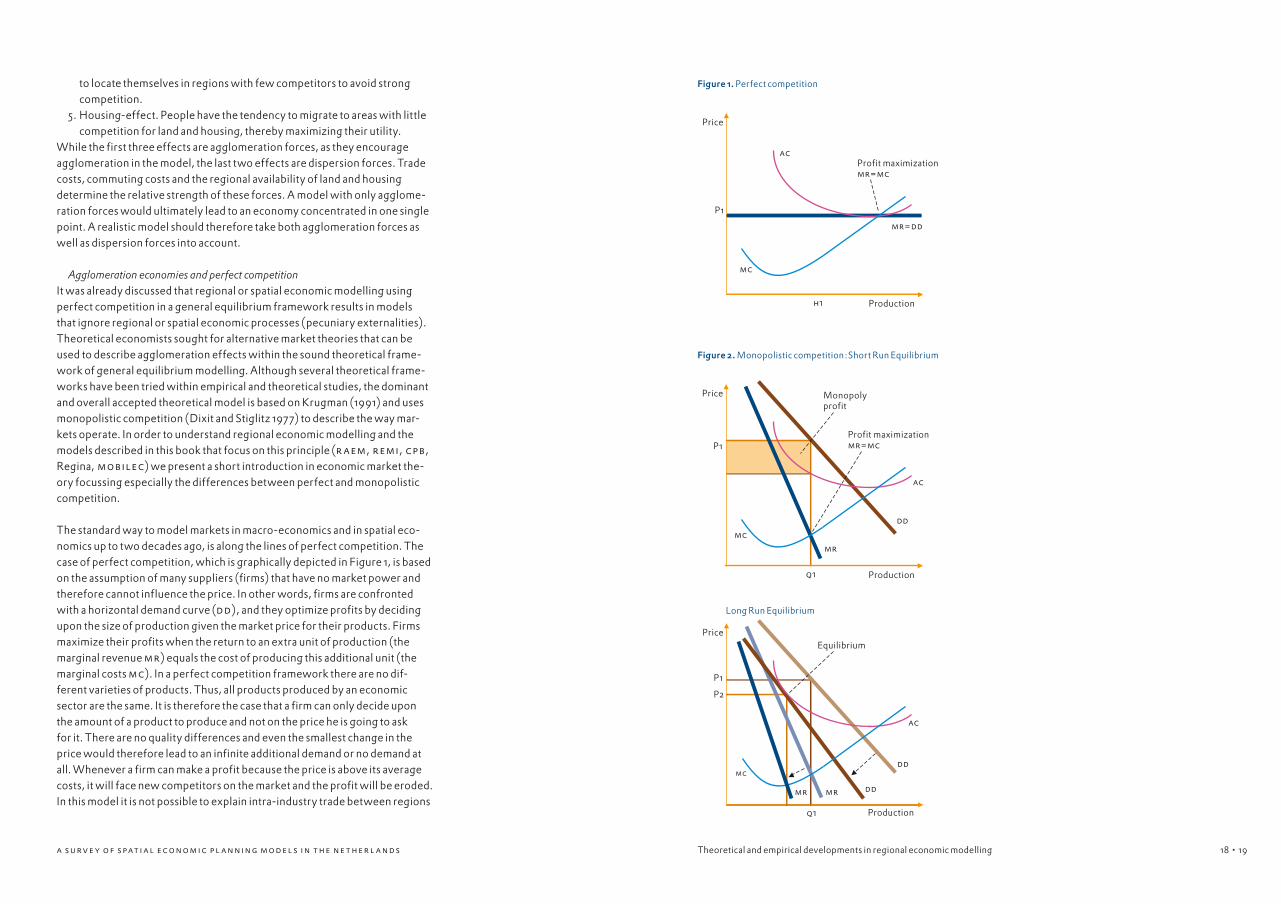
While the first three effects are agglomeration forces, as they encourage agglomeration in the model, the last two effects are dispersion forces. Trade costs, commuting costs and the regional availability of land and housing determine the relative strength of these forces. A model with only agglome-ration forces would ultimately lead to an economy concentrated in one single point. A realistic model should therefore take both agglomeration forces as well as dispersion forces into account.
Agglomeration economies and perfect competitionIt was already discussed that regional or spatial economic modelling using perfect competition in a general equilibrium framework results in models that ignore regional or spatial economic processes (pecuniary externalities). Theoretical economists sought for alternative market theories that can be used to describe agglomeration effects within the sound theoretical frame-work of general equilibrium modelling. Although several theoretical frame-works have been tried within empirical and theoretical studies, the dominant and overall accepted theoretical model is based on Krugman (1991) and uses monopolistic competition (Dixit and Stiglitz 1977) to describe the way mar-kets operate. In order to understand regional economic modelling and the models described in this book that focus on this principle (r aem, remi, cpb, Regina, mobilec) we present a short introduction in economic market the-ory focussing especially the differences between perfect and monopolistic competition.
The standard way to model markets in macro-economics and in spatial eco-nomics up to two decades ago, is along the lines of perfect competition. The case of perfect competition, which is graphically depicted in Figure 1, is based on the assumption of many suppliers (firms) that have no market power and therefore cannot influence the price. In other words, firms are confronted with a horizontal demand curve (dd), and they optimize profits by deciding upon the size of production given the market price for their products. Firms maximize their profits when the return to an extra unit of production (the marginal revenue mr) equals the cost of producing this additional unit (the marginal costs mc). In a perfect competition framework there are no dif-ferent varieties of products. Thus, all products produced by an economic sector are the same. It is therefore the case that a firm can only decide upon the amount of a product to produce and not on the price he is going to ask for it. There are no quality differences and even the smallest change in the price would therefore lead to an infinite additional demand or no demand at all. Whenever a firm can make a profit because the price is above its average costs, it will face new competitors on the market and the profit will be eroded. In this model it is not possible to explain intra-industry trade between regions
Theoretical and empirical developments in regional economic modelling
Price
ac
P1
h1 Production
mr=dd
Profit maximizationmr=mc
mc
x
x
Figure 1. Perfect competition
Price
ac
P1
q1 Production
dd
mr
Profit maximizationmr=mc
mc
x
x
Monopoly profit
Price
ac
P2
P1
q1 Production
dd
ddmrmr
mc
x
x
Equilibrium
xx
Figure 2. Monopolistic competition:Short Run Equilibrium
Long Run Equilibrium

20 a s u rv e y o f s pat i a l eco n om i c p l a nni n g mo d el s i n t he ne t her l a nd s • 2120
with non-zero transportation costs because consumers will always by the cheaper product. The model will therefore predict spatial specialization at the industry level with low transport costs or regional autarkies with high trans-port costs. The only possible way to incorporate intra industry trade in this model is therefore to define regional differences in production and turning intra-industry trade into inter-industry trade.
Agglomeration economies and imperfect competitionMonopolistic competition on the other hand is best explained using Figure 2. In the short run, the monopolistic firm faces a demand curve dd and sets its price such that it maximises profits, i.e. such that Marginal Costs (mc) equal Marginal Revenue (mr). The firm makes a profit per product equal to the difference between the price and the average costs. However, profits attract new entrants and shift every firm’s demand curve (dd) to the left. In the long run equilibrium all profits are eroded and the price equals the Average costs (ac). Monopolistic competition is generally modelled using the Dixit-Stiglitz (1977) approach, in which producers and consumers have a preference for variety. All these varieties are imperfect substitutes. The availability of more varieties allows producers to use a more roundabout production process via an increased variety of intermediate inputs. The increased diversity of inputs allows producers to use a more ‘roundabout’ production process and lowers unit costs at given input prices. This is a variant of the insight given by Ethier (1982). Consumer’s utility depends also on the availability of different varie-ties, which better fit their preferences.
Using this approach to model monopolistic competition gives us a long-run equilibrium with zero profits where the number of varieties is a function of the substitution elasticity and the fixed costs of production.2 This substitution elasticity represents the degree of competition and determines the slope of the demand function in Figure 2. Thus, the size of the substitution elasticity between varieties determines the number of varieties produced in every region and, as the number of varieties determines the size of the agglomera-tion effect, this parameter determines the size of the spatial economies of scale. This modelling framework can be used in the production function above, the investment function (Ethier 1982) and in the utility function of consumers. Besides production becoming more efficient also welfare increases when more product varieties are available in a region. In a monopolistic competition framework there are different varieties of products produced in all regions. There is therefore variety in production within and between regions. In a monopolistic framework there are (quality) differences between prod-ucts and small changes in the price therefore lead to limited changes in the demand. Every firm is a little monopolist and sets its price to maximize its profits. However, any profit attracts new entrants to the market, and in the long run all profits are eroded. In this model it is possible to explain intra- industry trade between regions with non-zero transportation costs because
consumers are interested in different varieties of products. Also agglomera-tion effects occur due to changes in the local supply of varieties. The model will therefore predict spatial specialization at the industry level for agglo-merations of industrial activity. It will also predict differences in productivity among regions and particular varieties of comparable goods are possibly produced in different regions. Thus, opposite to the case of the competitive equilibrium framework, there is no complete specialization.
Policy, spatial interaction and agglomerationAlthough the above theoretical framework gives us the possibility to explain stylised facts such as agglomerations and permanent different growth rates of regions, we also need to explain how governments may use these spa-tial interactions to stimulate economic growth or repair adverse economic effects. Any policy measure that changes the economic shape of a country affects regional economic growth and income distribution. This in turn, may trigger migration and lead to even stronger changes of the economic land-scape. The economic morphology of a country is here defined as the time and costs necessary to connect two points in space for economic purposes such as trade or commuting. Policy measures that affect this morphology are physical measures such as transport infrastructure, but also spatial non-neutral taxes or subsidies such as road pricing. The economic shape of a country is determined by facilities for housing and industry and the time and costs of travelling, trade, and networks, between living and industrial areas. Thus, the economic space of a country not only involves the transport of goods and people, but also the embeddedness of the firm in its environment via its customers and employees and their means of communication i.e. the telephone or the internet. The government may affect the economic shape of the country by, for instance, the construction of road and rail infrastructure that affects the costs of commuting, transporting goods from the factory to the shop, the costs of bringing the goods from the shop to home or bringing the consumer to the place of consumption and, the costs of business travel. However, also new communication infrastructure has an effect on the economic shape of the country by changing search costs for finding the best variety and improving the firms network with other firms in its surrounding. Other policy variables that change the economic shape of a country and which have a regional economic effect are those that influence the location of housing and industries. Housing gives the possibility for con-sumption and labour to be at a certain location, while industrial areas give the possibility to make use of this labour and have firms in a certain place. An important part of the effects of policy measures that affect the eco-nomic space in neg models will affect the regional economy via pecuniary effects such as agglomeration economies and dispersion economies. For instance, when a region becomes more accessible due to new infrastructure, productivity may increase by a more roundabout production process and cheaper inputs due to lower transport costs. At the same time utility of con-sumers increases if they can choose among more variety. This will attract
2. This condition is normally pre-
sented as the substitution elasticity
being a function of the variable and
the fixed costs of production.
Theoretical and empirical developments in regional economic modelling

22 a s u rv e y o f s pat i a l eco n om i c p l a nni n g mo d el s i n t he ne t her l a nd s • 2322
people from other regions and lead to a larger supply on the local labour market and thereby increased production. The overall effect on production may therefore be that productivity increases exponentially with a rise in the regional scale of operating. This is an example of pecuniary externalities such as introduced in the previous section.
Interregional trade and agglomeration effectsProduct markets play a crucial role in the effect of changes in the economic space on regional economic development. Product markets are affected by changes in transport infrastructure via regional trade and the labour market. The way product markets are affected by changes in transport infrastructure will be given below as an example how agglomeration effects influence spatial economic developments. The effects of a change in transport costs on product markets in a neg model with monopolistic competition and pecu-niary effects such as agglomeration economies are graphically presented in Figure 3. In this flow diagram the other markets, such as the labour market, are taken Ceteris Paribus. A change in transport costs changes the competitive position of different regions. Firms in a region where transport costs decrease due to a new road will see their products become more competitive (cheaper) on other regional markets, but see also product varieties from other regions become more competitive on the local market. Thus, on the local market the firm faces increased competition that will lead to a competitive disadvantage for local industry and may lead to a decline of productivity in the local region due to scale and scope effects. This decline of local productivity causes the relative price of imports to decrease even more which enhances this negative effect for the region (pecuniary externality). On other regional markets the firm faces the opposite effect. Here the firms’ products become cheaper causing demand and production to rise with positive scale and scope effects and thereby enhancing the firm’s competitive advantage over firms from other regions. Which of the two effects will be dominant depends on the relative dependency of a region to trade and the size of the local market. Consumers see their access to different markets and more varieties in- crease. As long as the above mentioned potential negative production effect is not too large, it is expected that they gain from the reduction in transport costs. Thus, here we see how a change in transport costs may cause changes in demand and production via scale and scope effects that will lead to both national generative and interregional distributive results. Moreover it was shown that this might lead to cumulative processes via pecuniary externalities that result in far stronger effects than those in models without agglomeration effects.
Externalities and the need for other theoretical frameworks and models
The New Economic Geography models include space, but are primarily based on economics. Although there are many overlapping interests, the neg modelling tradition is in many respects different from ‘old’ economic
geography, specifically in accepting general equilibrium models and disre-garding detailed and specific attributes of cities, regions and international relations. Especially the explanatory power of spatial externalities in terms of knowledge spillovers remains a black box until today (Van Oort 2004). But opening up the black box of the exact working of externalities comes at the cost of less structured and complete modelling (Van Oort 2004). Martin and Sunley (1996) mention, for instance, the differences in the weights of the factor levels of spatial scale and the acceptance of heterogeneous actors and non-economic (e.g.: psychological and socio-political) factors. Another important difference is the acceptance of general and specific spatial beha-viour and structures. ‘Old’ economic geography emphasizes the existence of heterogeneousness and specific situations where it is not always useful to work with that kind of models but with case-studies for cities, regions or international relations. In the neg approach, one of the main issues is the thesis that the forces converging in, or leading towards, an equilibrium state – increasing returns, economies of scale, monopolistic competition and the relation of transport costs and wages – are independent of scale (‘spa-tial scale-free processes’). In the words of Brakman et al (2001, p323): ‘By using highly stylized models, which no doubt neglect a lot of specifics about urban, regional and international phenomena, geographical economics is able to show that the same mechanisms are at work at different levels of spatial agglomeration’. The neg tradition distinguishes little to no variation in types of firms (sectors), lifecycles of firms (firm formation or incumbent firm growth) and scales within regional and urban space (Lambooy and Van
Theoretical and empirical developments in regional economic modelling
Scale & scope effects
Import cheaper
Export cheaper
Lower transport
costs and time
g
Scale & scope effects
Local intermediate and
consumptive demand
Higher local production
h
f
g g
Lower local production
i
g
f
i
Income and labour
market effects
National generative
effects
Interregional
distributive effects
g
f
h
g
i
f
i
i
g
Figure 3. Effects of changes in transport costs on product markets

24 a s u rv e y o f s pat i a l eco n om i c p l a nni n g mo d el s i n t he ne t her l a nd s • 2524
Oort 2005). This is what is called the ‘representative firm, region or city’ in neg analyses. Geographical and evolutionary economic theories and models explicitly depart from this, but have no closed theoretical framework to back-up their findings. Still they shed light on modelling details the neg will never be able to address (like the quality of labour, low spatial scales of analysis and the relation with mobility), and therefore are interesting in themselves. Both the ge- and economic geography conceptualizations build on location theory, especially on the concept of externalities or spillovers. Externalities or spillovers occur if an innovation or growth improvement implemented by a certain enterprise increases the performance of other enterprises without the latter benefiting enterprise having to pay (full) compensation. Spatially bounded externalities are related to enterprise’s geographical or network contexts, and are not related to internal firm performance. All discussions of spatial externalities link to a threefold classification, as made by Isard (1960) in which the sources of agglomeration advantages are grouped together as:
1. Internal increasing returns to scale. These may occur to a single firm due to production cost efficiencies realized by serving large markets. There is nothing inherently spatial in this concept other than that the existence of a single large firm in space implies a large local concentration of factor employment
2. Whether due to firm size or a large initial number of local firms, a high level of factor employment (labour demand) may allow the development of external economies within the group of local firms in a sector: localisation economies
3. Or the development of external economies available to all local firms irrespective of sector: urbanisation economies.
Localization economies usually take the form of Marshallian (technical) externalities whereby the productivity of labour in a given sector in a given city is assumed to increase with total employment in that sector. In short, they arise from labour market pooling, creation of specialized suppliers and the emergence of technological knowledge spillovers. The strength of local externalities is assumed to vary, so that these are stronger in some sectors and weaker in others. The associated economies of scale comprise factors that reduce the average cost of producing commodities. External scale econo-mies apply when the industry in which the firm belongs (rather than the firm itself) is large. Under further assumptions on crowding (congestion costs that increase with population triggers dispersion), perfect product and labour mobility within and between locations and the influence of large agents, an urban system is composed of (fully) specialized cities, provided that the initial number of cities is large enough. Once cities exist, urbanisation economies become important as well. The concept of agglomeration externalities in this framework is used by both regional economists and the neg (Brakman et al. 2001). Urbanisation and localisation economies are essentially investigated at the urban and agglomerated level (Frenken et al. 2004). Within the ‘old’ geography, especially ‘untraded interdependencies’ that function as externalities and spillovers are the focus of geographical research
recently (Sjöberg and Sjöholm 2002). In geography, by history, there has always been a much larger emphasis on spatial differentiation and on the interaction of the relevant urban or regional environment with locational choices made by individual firms and investors than in the neg models. More general, the main differences between the neg context of analysis and the geographical one is the role that the treatment of individual choice by entrepreneurs and behaviour play in them. The influential behavioural geographical literature (Webber 1972) focuses on rational choice, incomplete information, limited cognitive capacities of entrepreneurs and differences in information absorption in life stages of firms. Especially newly founded firms (starting entrepreneurs) have limited experience in their business, and locational choices (concerning first location, in-situ growth or movement) will be limited to certain information-dense regions or cities where (trans-action) cost minimalisation and profit optimising opportunities are thought to be optimal. Regionally, the living and working location of newborn entre-preneurs will not diverge much. Large urban agglomerations are often better incubator places than other locations in this respect. Relative large product markets, a diverse supply of input factors and common infrastructures are important factors for urban location. The stylised fact that the life phase of (especially new and young) firms in different industries is highly influential on agglomeration is largely ignored in neg models – the ‘representative firm’ is common in this theory. Theories focusing on choice and behaviour can be extended to meso- and macro economic growth theories, as in evolutionary economics. Structures are more than the aggregation of individual choices, it is the result of many interactive processes (Boschma and Frenken 2003). Evolutionary economic theory focuses on the creation of new spatial structures, and less on explain-ing equilibrium sates. Within the same spatial and institutional context, firms and entrepreneurs come to different location behaviour. In evolutionary economic theory, ‘new’ industrial locations might occur by means of chance or ‘catastrophes’ (usually lead by the introduction of new technologies). Neo-Schumpeterian, endogenous growth (especially caused by innovation) can cause a process of creative destruction in the ‘old’ agglomerations of economic activity (like the Ruhr-region in Germany) and can develop relative new concentrations elsewhere (like Silicon Valley). Still, after a certain period, agglomerated location occurs on the macro-level again: externalities and spillovers become localised and regional clustering and co-location is profitable (again) for firms. From then on, path-dependency becomes important in explaining persisting agglomeration of economic activity. Both ‘old’ geographical theories and the neg models cannot deal with these phenomena in one single conceptualisation like evolutionary economics can.
Theoretical and empirical developments in regional economic modelling
References
Arrow, K.J. and Debreu, G. (1954),
‘Existence of an equilibrium for a com-
petitive economy’, Econometrica, Vol. 22:
265–290.
Baldwin, R., R. Forslid, P. Martin,
G. Ottaviano and F. Robert-Nicoud
(2003), Economic geography and public
policy, Cambridge Mass.: The mit Press.

26 • 2726 a s u rv e y o f s pat i a l eco n om i c p l a nni n g mo d el s i n t he ne t her l a nd s
The remi model for
the Netherlands
Boschma, R.A. and K. Frenken (2003),
‘Evolutionary economics and industry
location’, Review for Regional Research 23:
183–200.
Brakman, S., H. Garretsen and C. van
Marrewijk (2001), An introduction to geo-
graphical economics, Cambridge: University
Press.
Bröcker, J. (2000), ‘Trans-European
Networks: results from a spatial cge anal-
ysis’, pp. 141–159 in : F. Bolle, M. Carlberg
(eds.), Advances in behavioral economics,
Heidelberg: Physica.
Dixit, A.K. and J.E. Stiglitz (1977),
‘Monopolistic competition and optimum
product diversity’, The American Economic
Review 67: 297-308.
Ethier, W.J. (1982), ‘National and inter-
national returns to scale in the modern
theory of international trade’, American
Economic Review 72:389–405.
Frenken, K, F.G. van Oort, T. Verburg
& R. Boschma (2005), Variety and regional
economic growth in the Netherlands, The
Hague: Ministry of Economic Affairs.
Fujita, M., P. Krugman and A.J. Venables
(1999), The spatial economy. Cities, regions
and international trade, Cambridge Mass.:
The mit Press.
Fujita, M. and J.F. Thisse (2001),
Economics of agglomeration. Cities, industrial
location and regional growth, Cambridge:
University Press.
Hahn, F. (2002), ‘On the Possibility of
Economic Dynamics’, pp. 221–230 in:
C.H. Hommes, R.Ramer and C.A. Wit-
hagen (eds.), Equilibrium, markets and
dynamics, Berlin: Springer.
Heyma, A. and J. Oosterhaven (2005),
‘Social cost-benefit analysis and spatial-
econometric models in the Netherlands’,
pp. 153–175 in: Frank van Oort, Mark
Thissen & Leo van Wissen (eds.) A survey
of spatial economic planning models in
the Netherlands. Theory, application and
evaluation, Rotterdam/The Hague: NAi
Publishers, rpb.
Isard, W. (1960), Methods of Regional
Science, Cambridge Mass.: The mit Press.
Krugman, P.R. (1991), ‘Increasing
returns and economic geography’, Journal of
Political Economy 99: 483–99.
Krugman, P.R. and M. Obstfeld (1991),
International Economics: theory and policy,
New York: HarperCollins.
Lambooy, J.G. & F.G. van Oort (2005),
‘Agglomerations in equilibrium?’, in: S.
Brakman & H. Garretsen (eds.), Location
and Competition, London: Routledge.
Martin, R. and P. Sunley (1996), ‘Paul
Krugman’s geographical economics and
its implications for regional development
theory: a critical assessment’, Economic
Geography, 72: 259–92.
Oort, F.G. van (2004), Urban growth and
innovation. Spatially bounded externalities in
the Netherlands, Aldershot: Ashgate.
Oosterhaven, J. T. Knaap, C. Ruygrok &
L. Tavassy (2001), On the development of
ream: The Dutch spatial general equilibrium
model and it’s first application to a new
railway link, paper presented on the 41th
Congress of the European Regional Science
Assocation.
Sjöberg, O. and F. Sjöholm (2002),
‘Common ground? Prospects for integra-
ting the economic geography of geog-
raphers and economists’, Environment and
Planning A, 34: 467-486.
Staret, D. (1978), ‘Market allocation of
location choice in a model with free mobil-
ity’, Journal of Economic Theory 17: 421–436.
Thissen, M.J.P.M. (2004) ream 2.0.
A Regional Applied General Equilibrium
Model for the Netherlands, Working paper,
Delft: tno Inro.
Webber, M.J. (1972), Impact of uncer-
tainty on location, Cambridge Mass.: The
mit Press.

28 • 2928
the r emi model for the nether l ands Gerbrand van Bork & Fred Treyz
IntroductionWhy the remi-nei model?
In recent years there has been an upswing in the need of policy-makers to gain insight into the economic impact and costs and benefits of policy. At the same time there is an ongoing debate on the indirect economic effects of infrastructure projects in the light of the oei guidelines for cost-benefit anal-ysis (see the contribution of Heyma and Oosterhaven in this book). It is these developments that have led the research consultants of ecorys to review its own tools for quantifying economic impact. Many of the existing tools (such as I/O analysis, shift-share regression, labour market modules) are only suitable for quantifying partial economic impact, hence we felt the need to improve our tools for this purpose. The search has led to the development by ecorys, in cooperation with remi Inc., of the remi-nei model for the Netherlands.
Aim of the remi-nei model and possible applicationsBecause of its features the remi model is particularly suitable for quantify-ing the impact of policies on the regional and national economy. It can also be used to construct long-term economic scenarios for regions and the Netherlands as a whole. It is less suitable for short-term forecasting, as it is not based on cyclic time-series regressions.
Possible applications of the model are to assess the economic impact of poli-cies in the fields of:
· Infrastructure (rail, road, waterway)· Mainports (Port of Rotterdam, Schiphol airport)· Spatial investment (‘Nieuwe Sleutelprojecten’, business estates etc.)· Labour market policies (training, social security contributions)· Energy (cost savings programmes etc.)· The environment
Origin of the remi-nei modelThe original version of the remi model was developed at the University of Massachusetts in 1977. In later years it was extended into a model that could be generalized for all states and counties in the us under a grant from the National Cooperative Highway Research Program. Since 1977 a vast litera-ture of international articles has been produced on the model and its exten-sions and the estimation of equations (see References). The model has now been developed for several regions in Europe, as well as the Netherlands. It has recently been developed for the uk (by ecotec), Scotland, Belgium,
The remi model for the Netherlands

30 a s u rv e y o f s pat i a l eco n om i c p l a nni n g mo d el s i n t he ne t her l a nd s • 3130
Southern Italy and Spain (by the European Commission) and North Rhine Westphalia (by rwi).
The remi-nei modelTheory
remi/ecorys is a regional economic model with new economic geography elements and general equilibrium elements. It is partly a general equilibrium model, because of optimising behaviour of consumers, producers and work-ers. However the markets in the model do not immediately arrive at new equilibria. Complete input-output relationships are incorporated in its struc-ture, and dynamic responses are estimated using econometric approaches. It has been developed as an applied, structural forecasting and policy analysis model, thus providing a comprehensive description of economic flows, industry relationships, and demographic issues. The microeconomic foundations of the remi macroeconomic model are described in Fan, Treyz & Treyz (2000). This theoretical model provides a prototype for incorporating the new economic geography in the applied remi framework, which was initially implemented in 1980 and has been continually updated and developed. The new economic geography industry structure is monopolistic competition as explained in the introduction to this book. Given this set of assumptions, cities of differing sizes and industry struc-tures form endogenously. Equilibrium depends not only on the initial con-ditions but also on the speed of adjustment. As we apply this to the empirical remi model, the initial economic conditions represent the actual economic and demographic structure of the Netherlands, yet respond to changes in agglomeration economies.
Comparison with other modelsWith its complete input-output framework remi has a great deal in common with other models for the Netherlands that have a strong input-output basis. remi has been systematically compared to hermin, Quest II, and Venables and Gasiorek as models internationally available used to evaluate European Union investments (Treyz and Treyz 2004). Venables and Gasiorek provide a strong theoretical basis in terms of new economic geography, and its build-ing blocks are individual firms. Quest II is a Multi-Country Business Cycle and Growth model with a strong basis in neo-classical economic theory, assuming rational and foresighted decisions by economic actors; it is limited when it comes to national and international analysis, as it does not provide for local/regional economies. hermin is theoretically based on a two-sector, small open economy model with a Keynesian component: the coefficients and functional form vary depending on the implementation, and the modelling approach considers time-series data in determining its specification for any particular country.
Output
ihState & Local
Government Spending
Consumption
Investment
Exports Real Disposable Iincome
1. Output
h
i i
h
Employ-
ment
iLabour/Output Ratio
Optimal
Capital
Stock
h
f
Inter-
national
Market
Share
i
Domestic
Market
Share
i
5. Market Shares
Population
iLabour
Force
Migration h
3. Demographic
g
2. Labour & Capital Demand
Participa-
tion Rate
h
i
i
i
4. Wages, Prices & Production Costs
Wage Rate
Consumer
Price Deflator
Employment Opportunity h
Housing Price h hReal Wage Rate
Composite Wage Rateh Production Costs
iComposite Prices
h
g
hh
i i
h
h
h
h
h
h
h
g
h
h
The remi model for the Netherlands
Figure 1. remi Model Linkages (excluding Economic Geography Linkages)

32 a s u rv e y o f s pat i a l eco n om i c p l a nni n g mo d el s i n t he ne t her l a nd s • 3332
Structure of the remi-nei modelThe remi model consists of thousands of simultaneous equations while having a relatively straightforward structure. The overall structure of the model can be summarized in five main blocks representing the various mar-kets in the model: (1) output and demand on the market for goods and servi-ces, (2) labour and capital demand on labour market and capital market, (3) population and labour force (the labour market), (4) wages, prices and costs, and (5) market shares (the market for goods and services). Figure 1 shows the blocks and their key interactions.
The regional final demand from consumers and the regional output of firms are determined in the output block, which essentially describes the regional markets for goods and services. The labour and capital demand block con- tains the equations for the demand for labour (on the regional labour markets) and the demand for capital (the capital goods market). Regional output and wages determine the demand for (a) labour and (b) capital goods. The regional labour supply is dependent on population (age structure, sex) and interregional migration (the demographic block). In the wages, prices and cost block, wages are influenced by the supply and demand of labour, and prices by production costs. These wages, production costs and prices deter-mine the market shares of regions compared with other regions in the Netherlands and in the international market. Regions with lower cost and price levels will have a larger market share and therefore bigger output than other regions. A more detailed description of the blocks in the model is given in Appendix 1.
The main (regional and national) markets described in the model are:· The market for goods and services (regional supply and demand for
goods and services)· The labour market (labour supply and demand)· The market for capital goods (investment)· The housing market (the housing price equation)
The land and real estate markets (apart from housing prices) are not included in the model.
Important exogenous variables in the model are national forecasts of popu-lation, exports and productivity, using the Netherlands Bureau for Economic Policy Analysis (cpb) figures for the long-term European Coordination sce-nario. Other exogenous variables are transport costs, energy prices and other business costs, commuting costs, taxes and social security contributions. The model has many endogenous variables, for example:
· Gross regional product and gross national product (by industry)· Exports, productivity· Employment (by industry) and unemployment· Participation rates and the labour force· Wages, prices and housing prices
In the recent new economic geography literature, the advantages and disadvantages of agglomeration can influence a region’s productivity and economic growth. Advantages of agglomeration are e.g. knowledge spill-overs, variety of intermediate and consumer goods and variety of labour sup-ply; disadvantages are congestion, rising real estate prices etc. The model incorporates the following aspects of the new economic geography, which were also discussed in the introduction to this book. Variety of intermediate goods and services (commodity access index). More intermediate goods and services increase productivity in the model, the idea being that more choice gives firms more possibilities to optimize inputs. Variety of consumer goods and services. In remi more variety of consumer goods has a positive impact on migration: the idea is that the beneficial effect on consumers of having more access to consumer goods (services of hotels, restaurants etc.) makes regions more attractive. Labour access. Better access to specialized labour thanks to a bigger pool of workers enhances the productivity of firms in the model. The principle is that the ‘broader labour market’ enables firms to select better workers according to their needs, improving the qualitative match on the labour market. The model applies this concept by allowing more labour supply to have a positive impact on productivity. Housing prices. Increasing population and per capita income have a posi- tive impact on real estate prices in the model; this increases the cost of pro-duction, however, and therefore has a negative effect on regional production growth.
Estimation and implementationThe remi-nei model represents the Netherlands as seven regions: North Holland (South) (the ‘corop’ regions of Greater Amsterdam, the Zaanstad region, the Gooi & Vecht region, Ijmond and Haarlem); Flevoland (the prov-ince); Utrecht (the province); Greater Rotterdam (the corop region); the Rest of South Holland, Southeast Brabant (the corop region) and the Rest of the Netherlands. Key data used in the model are the national input-output table, the con-sumer sector table and wages and income data from the National Accounts of the Netherlands, published by Statistics Netherlands (cbs). Data include wages and salaries and employment for 24 industries, personal consumption expenditure, household income, taxes and disposable income, and personal income. Demographic data from the cbs includes population by single year of age, numbers of births and deaths, international and interregional migration, and natality and survival rate forecasts. Additional data from Eurostat was used to calculate labour force participation rates by age and sex and to fore-cast national participation rates. Trade flows by industry were calculated for the 40 corop regions, which were then aggregated to produce trade flows for the six regions in the model. Trade flows for a given industry are based on regional output, demand, and the distance to other regions. A region-specific distance decay parameter
The remi model for the Netherlands

34 a s u rv e y o f s pat i a l eco n om i c p l a nni n g mo d el s i n t he ne t her l a nd s • 3534
determines the extent to which trade occurs in a particular industry. These universal parameter estimates are based on cross-sectional time-series data for over 3,000 us counties over a ten-year period, to determine the decay of market shares across distance. This dynamic approach requires a large time-series, cross-sectional data set that is not available for the Netherlands. (Data is also not available for survey-based approaches, particularly in the case of the non-manufacturing industries, which account for over 85% of Dutch employment). Further developments in the model will include distance decay parameter estimates using available European data. A guiding principle in the design of remi is maintaining a theoretically consistent framework. The model is calibrated to the data for the particular national, regional, or multi-regional configuration. Parameter estimates are typically based on panel data for a large number of regions over many years. The use of panel data allows for robust parameter estimates within a consis-tent structural methodology. Estimates based on individual time-series data for a single region do not provide a sufficient statistical basis for consistent model estimation, hence models based on single time series often have ad hoc formulations, with variables added or discarded based on their statistical validity for a limited set of observations. In order to maintain key dynamic responses that are supported by the data, remi-nei is constructed using the best available estimates based on available panel data. To some extent this means relying on estimates based on research into individual equations for the us using data sets and procedures that have been conducted during the 24-year development of remi, including exten-sive re-estimation. Migration in response to wage rate and employment changes is based on the largest European data set available, using data for Germany. This provides for a major structural difference between us and European labour markets. Fixed effects for regional migration are calibrated specifically for each of the Dutch regions. Estimates of distance decay parameters, a central aspect of the regional dimension of the model, will be developed using available European data. Long-term estimated export elasticities calculated by the cpb are also under consideration for incorporation in the model.
A practical case study using remi-neiPolicy relevance and the relationship with cba
As stated earlier, remi-nei is mainly a tool for measuring impact, although it can also be used for scenario construction. In this respect it can give policy-makers a good insight into the economic impact of different policies. It can be used for Cost Benefit Analysis (cba), but the researcher has to adapt outputs from the model for this purpose. It gives as output the total economic impact of policies: this is the sum of direct and indirect impacts (cba terminology). The researcher then has to decide whether the indirect impacts are additional to the direct impacts of policies. The regional structure in the model enables it to give an insight into the regional distributional effects of policies. The output from the model includes agglomeration or scale effects, thanks to the new geography elements.
Application to the Almere-Haarlemmermeer corridorremi was recently used to carry out a cost-benefit analysis of urbanization alternatives for the Randstad area and infrastructure in the Haarlemmermeer-Almere corridor. This study was done for the Dutch Ministries of Housing and Environment, Transport, Finance, Agriculture and Economic Affairs. In this example we give some information on the impact of the Haarlemmermeer-Almere corridor, which will need new infrastructure by 2010 because of the growth of housing and economic activity in Almere and the Haarlemmermeer area. There are two proposed alternatives for the new infrastructure in the Haarlemmermeer-Almere corridor:
· Highway max.: more extension of major highways and regional motorways planned than increase in public transport capacity (rail)
· Public transport max.: less enlargement of major roads and regional motorways planned and more public transport capacity
The direct impacts of these two alternatives are reductions in travel time for commuters and business and leisure travellers. The transport model for the North Randstad area of dhv was used to calculate these induced trans-port effects (transport flows and time savings). The travel time reductions were translated into transport cost savings for commuters and businesses as inputs to remi. As the input variable to the model we have used the matrices of transport cost for commuters and businesses between regions. Figure 2 shows the mechanism for assessing the impact on the economy of changes in transport costs. There are two ways in which a change in transport costs has an impact on the regional economy in remi:
· A reduction in transport costs for businesses causes lower prices and therefore an increase in the region’s market share, in turn leading to higher production and employment in the region.
Travel cost reduc-
tion commuters
Transportation cost
reduction business
Change in
accessability
f
i
Improved
labour access
Price reduction
companies
f
f
fProductivity
gain
Increase market
share regionf
f
Increase in
production and
employment
f
The remi model for the Netherlands
Figure 2. remi mechanism for modelling impacts of changes in transport costs on the
regional economy

36 a s u rv e y o f s pat i a l eco n om i c p l a nni n g mo d el s i n t he ne t her l a nd s • 3736
· A reduction in travel costs for commuters improves companies’ access to the labour supply, giving them a wider choice of employees, giving rise to a better – qualitative – match on the labour market. This makes companies in the region more productive and brings about an increase in their market shares in other regions and foreign countries. Exports, production and employment therefore go up.
ResultsThe results from the transport model, translated into reductions in transport costs, yielded the following employment impacts of the Highway maximum alternative. As figure 3 shows, the North Holland (South) region (Greater Amsterdam, Haarlemmermeer) gains a large increase in employment. The Flevoland re-gion (where Almere is situated) and the Rest of the Netherlands, on the other hand, experience a decrease in employment. The infrastructure between Flevoland (Almere) and North Holland (North) causes reductions in trans-port costs in both North Holland (North) and Flevoland. When the transport costs in more regions change because of infrastructure changes, however, the relative changes affect the impacts on the regional economy: North Holland (North) has a larger reduction in travel costs than Flevoland. This is reinforced by the fact that the reduction is less important to the industry mix in Flevoland (which has a lower share of manufacturing).
A new insight from the model is the effect of reductions in commuting costs on productivity, which has been neglected in many previous studies on infra-structure. Also new are the agglomeration effects, which are quantified for the first time. Finally, the model shows that some regions might gain from infrastructure changes, but others might lose, depending on the relative decrease in costs and market shares. More details can be found in ecorys (2003).
Conclusions and further research
Evaluation of the modelecorys researchers tested the first design of remi-nei for plausibility in various ways. First they checked all the data. Secondly, they compared the model’s baseline forecast with the cpb’s long-term ec scenario for the Dutch economy and corrected it on this basis. Thirdly, they tested it with a series of projects (Maasvlakte 2, the Randstad Transrapid Circle, Rotterdam nsp). The direct impacts of these projects from previous studies were used as inputs to the model. The magnitude of the economic results from the model was com-pared with previous economic impact studies and the literature, and import-ant coefficients in the model were compared with those in other models. Finally, a plausibility check of the mechanisms was carried out. After each test the model was adapted if coefficients were out of line with other insights and the magnitude of results was not in line with the literature and previous
studies. cpb gave a second opinion, making important recommendations on the model. This led to an agenda for future research (see below).
ConclusionThe remi model for the Netherlands is a worthwhile tool for quantifying the economic impact of policies. It incorporates mainstream economic insights and elements from the new geography literature. Economic impacts in the Dutch model are based on the direct impact of policies, ensuring a solid causal mechanism for the quantification of impacts. A good understanding of the quantitative economic impact of policies is important if policy-makers are to have a solid basis on which to make decisions.
Further researchHaving applied the model a number of times, we envisage the following pos-sibilities for further research in order to improve it.
· Adding more regions to the model to provide more regional detail in remi-nei. Regions are currently added when requested by our clients.
· Re-estimate some labour participation and price elasticity coefficients for the Dutch labour market and goods market.
· Introduce reservation wages (unemployment benefits) in the labour participation equations. The reaction of labour supply to wage changes will be lower than in the us because of unemployment benefits. In order to capture this behaviour on the Dutch labour market we need to introduce reservation wages into the model.
· Commuting patterns as an endogenous variable. Commuting patterns between the regions are currently exogenous in the model, which
C4 F3
-4000
-2000
0
2000
4000
6000
8000
Groot-Rijnmond
Utrecht
Overig Zuid Holland
Noord Holland zuid
Flevoland
Overig Nederland
20302028202620242022202020182016201420122010
The remi model for the Netherlands
Figure 3. Employment impacts of the Highway max. (5N) alternative
Greater Rijnmond
Other South Holland
Utrecht
North Holland South
Flevoland
Other Netherlands

38 a s u rv e y o f s pat i a l eco n om i c p l a nni n g mo d el s i n t he ne t her l a nd s • 3938
means that commuting does not act as an equilibrium-bringing force on the regional labour market in remi. Because of the importance of commuting to regional labour markets in the Netherlands, we think it is necessary to introduce commuting as an endogenous variable in the model.
· Allow for more disadvantages of agglomeration (new geography elements). At present the only negative agglomeration force in the model is real estate prices. Further research into negative urbanization factors is another interesting option that could improve the model.
appendix 1. block s in the r emi-nei model
This appendix describes the five building blocks and the relationships within them.
Block 1. Output and demand on the market for goods and services. Key Endogenous
Linkages in the Output
This block contains the output, demand, consumption, investment, govern-ment spending, import and export equations. Output for each industry in the home region is determined by industry demand in all regions in the nation, the home region’s share of each market, and international exports from the region. For each industry, demand is determined by the amount of output, con-sumption, investment and capital demand in that industry. Consumption depends on real disposable income per capita, relative prices, differential income elasticities and population. Input productivity depends on access to inputs, as the larger the choice set of inputs, the more likely that the input with the specific characteristics required for the job will be formed. In the capital stock adjustment process, investment occurs to fill the difference between optimal and actual capital stock for residential, non-residential, and equip-ment investment. Government spending changes are determined by changes in the population.
8. Commodity Access
Index
10. Change in Local
Supply
g
Composite
Price
(Block 4)
7. Intermediate
Input s
9. Intermediate Input
Productivity
3. Consumption6. Output5. State and Local
Government
Spending
4. Investment
h
g
g
h
h
g
h
ghh
Economic
Migrant
(Block 3)
Population
(Block 5) h
h
h
h
Share of Domestic
Markets (Block 4)
g
Share of
International
Markets (Block 4)
Employment
(Block 2)
g g
hMarket
Share
(Block 5)
h
Population
(Block 5)
Consumer
Prices
(Block 4)
hWage Rate
(Block 4)
(Not shown) Commuter
Income or Outflow;
Property Income;
Transfer; Taxes;
Social Security Payments
g
2. Real Disposable
Income
1. International
Exports
The remi model for the Netherlands
h
Optimal vs.
Actual Capital
Stock (Block 2)

40 a s u rv e y o f s pat i a l eco n om i c p l a nni n g mo d el s i n t he ne t her l a nd s • 4140
Block 2. Labour and Capital Demand
The labour and capital demand block includes the determination of labour productivity, labour intensity and the optimal capital stocks. Industry-specific labour productivity depends on the availability of workers with differentiated skills for the occupations used in each industry. The occupational labour sup-ply and commuting costs determine firms’ access to a specialized labour force. Labour intensity is determined by the cost of labour relative to the other factor inputs, capital and fuel. Demand for capital is driven by the optimal capital stock equation for both non-residential capital and equipment. Optimal capital stock for each industry depends on the relative cost of labour and capital, and the employment weighted by capital use for each industry. Employment in private-sector industries is determined by the value added and employment per unit of value added in each industry.
Block 3. Population and Labour Force
The population and labour force block includes detailed demographic infor-mation on the Dutch regions. cbs population data is used for age, gender and ethnic category, with birth and survival rates for each group. The size and labour force participation rate of each group determines the labour supply. An important feature of the model is that participation rates are endogenous. These vary widely across age, gender, and ethnic category, hence the labour force depends in large part on the population structure of the region. These participation rates respond to changes in employment relative to the potential labour force and to changes in the real after-tax wage rate. In a subsequent version of the model we should like to use the reservation wage (wages minus unemployment benefits) instead of the real wage. Migration includes retirement, military, international and economic migration. Economic migration is determined by the relative real after-tax wage rate, relative employment opportunity and consumer access to variety in com-parison to other regions. Migration, economic or non-economic, also varies widely across population groups in the model.
1. Economic
Migration
h
h
g
h
Employment Oppor-
tunity (Block 4)g
h h
h
g
4. Employment
to Potential
Labour Force
6. Labour Force
2. Population
5. Participation
Rate
3. Potential Labour
Force
h
Wage Rate
(Block 4)
h
Local Government
Spending (Block 1)
Housing Price
(Block 4)
h
Employment
Opportunity
e/lf (Block 4)
Relative
Real Wage
Rate(Block 4)
Commodity
Access Index
(Block 1)
g
Residentially
Adjusted
Employment
(Block 2)
Relative
Real Wage
Rate
(Block 4)
The remi model for the Netherlands
8. Actual
Capital
Stock
Invest-
ment
(Block 1)
7. Optimal Non-
Residential
Capital Stock
9. Gap between
Actual and
Optimal Stock
h
g
Real Dis-
posable
Income
(Block 1)
h
h
Wage Rate
vs. Capital
(Block 4)
g
Real Disposable
Income (Block 1)
Calculated
Earnings (Block 1)
Composite
Wage Rate
(Block 4)
g
10.Optimal
Residential
Capital Stock
i
h
g
5. Factor Price
Substitution
Effects
6. Capital
Intensity
3. Occupational
Employment
4. Labour Access
Index by
Occupation &
Industry
g
g
1. Labour
Productivity
g
2. Industry Employment
h
h
h
Wage Rate
(Block 1)
g
g
h
g g
Output
(Block 1)

42 a s u rv e y o f s pat i a l eco n om i c p l a nni n g mo d el s i n t he ne t her l a nd s • 4342
Block 4. Wages, Prices and Costs
This block includes delivered prices, production costs, equipment cost, the consumption deflator, consumer prices, the price of housing, and the wage equation. Economic geography concepts account for the productivity and price effects of access to specialized labour, goods and services. These prices measure the price of industry output, taking access to produc-tion locations into account. This access is important because of the speciali-zation of production that takes place within each industry, and because the transport and transaction costs of distance are significant. Composite prices for each industry are then calculated based on the production costs of the sup-plying regions, the effective distance to these regions, and the index of access to the variety of output in the industry relative to access by other uses of the product. The cost of production for each industry is determined by the costs of labour, capital, fuel and intermediate inputs. Labour costs reflect a produc-tivity adjustment to account for access to specialized labour, as well as under-lying wage rates. Capital costs include those of non-residential structures and equipment, while fuel costs comprise those of electricity, natural gas and residual fuels. The consumption deflator converts industry prices to prices for consump-tion commodities. For potential migrants, the consumer price is additionally calculated to include housing prices. Housing price changes from their initial level depend on changes in income and population density.
Wage changes are due to changes in labour supply and demand conditions and changes in the national wage rate. Changes in employment opportunities relative to the labour force and occupational demand determine wage rates by industry.
Block 5. Market SharesThe market shares equations measure the proportion of the local and export markets that are captured by each industry. These depend on relative produc-tion costs, the estimated price elasticity of demand, and the effective distan-ces between the home region and each of the other regions. The change in the share of a specific area in any region depends on changes in its delivered price and the quantity it produces compared with the same factors for com-petitors in that market. The share of local and external markets then drives exports from and imports into the home economy.
appendix 2 . indus tr ies in the r emi-nei model
Sectors1. Agriculture, forestry and fisheries2. Mining3. Food industry4. Textile and leather industry 5. Graphical industry6. Oil industry7. Chemicals8. Rubber and plastics industry9. Metal industry10. Machine industry 11. Electrotechnical industry12. Transport equipment industry13. Wood, furniture and games industry14. Electricity, gas and water supply15. Construction16. Trade and repairs17. Hotels, cafes and restaurants18. Transport, storage and communication19. Financial services20. Rental and trade in real estate21. Commercial services22. Health and welfare23. Services (other)24. General Government
The remi model for the Netherlands
h
fh
i
3. Composite
Wage Rate
1. Employment
Opportunity
e/lf
Labour Access Index
by Occupation &
Industry (Block 2)
h
Share of Inter-
national Exports &
Imports (Block 5)
Share of Domestic
Markets (Block 5)
h
g
Residentially
Adjusted Employ-
ment (Block 2)
h2. Wage Rate
g
g
8. Housing Price
i
6. Consumer
Pricesf
i
g
f
9. Consumer
Prices Including
Housing Price
5. Production
Costs
4. Composite
Input Costs
7. Real Wage
Rate
10. Real Relative
Wage Rate for
Migrants
i
h
f Input Access
Productivity Effect
(Block 1)
Change in
Population
Density (Block 3)
hChange in Real
Disposable
Income
Migrants
(Block 3)
f
hLabour Force
i
Occupational Em-
ployment (Block 4)
h

The cpb Regional Labour
Market Model
A tool for long-term scenario
construction
References
cpb (1997), Economie en Fysieke Omgeving,
Den Haag: Sdu Uitgevers.
cbs, various sources (Statline, National
Accounts).
ecorys (2003), Economische Effecten
Corridor Haarlemmermeer-Almere.
Fan, Wei, Frederick Treyz and George
Treyz (2000), ‘An Evolutionary New
Economic Geography Model’, Journal of
Regional Science, Vol. 40(4): 671–695.
Fujita, Masahisa, Paul Krugman, and
Anthony J. Venables (1999), The Spatial
Economy: Cities, Regions, and International
Trade. Cambridge, ma: mit Press.
Greenwood, Michael. J., Gary L. Hunt,
Dan S. Rickman, and George I. Treyz (1991),
‘Migration, Regional Equilibrium, and the
Estimation of Compensating Differentials’,
American Economic Review, Vol. 81(5):
1382–1390.
Rickman, Dan S., Gang Shao, and George
Treyz (1993), ‘Multiregional stock adjust-
ment equations of residential and nonresi-
dential investment in structures’, Journal of
Regional Science, Vol. 33(2): 207–219.
Treyz, Frederick, and George I. Treyz,
(1997), ‘The remi Multi-Regional u.s.
Policy Analysis Model’, paper presented
at the North American Regional Science
Association Meetings.
Treyz, George I. (1993), Regional Economic
Modeling: A Systematic Approach to
Economic Forecasting and Policy Analysis,
Norwell, ma: Kluwer Academic Publishers.
Treyz, George I., Ann F. Friedlaender,
and Benjamin H. Stevens (1977),
Massachusetts Economic Policy Analysis
Model.
Treyz, George I., and Lisa M. Petraglia
(2001), ‘Consumption Equations for a
Multi-Regional Forecasting and Policy
Analysis Model’, Regional Science
Perspectives in Economic Analysis, Elsevier
Science B.V.: 287–300.
Treyz, George I., Chris G. Christopher,
Jr., and Chengfeng Lou (1996), Regional
Labor Force Participation Rates, Regional
Economic Models, Inc. remi Economic
Model Documentation.
Treyz, George. I., Dan S. Rickman, Gary
L. Hunt, and Michael J. Greenwood (1993),
‘The Dynamics of U.S. Internal Migration’,
The Review of Economics and Statistics, Vol.
lx xv, No. 2, May 1993: 209–14.
Weisbrod, Glen, Donald Vary, and
George Treyz (2001), ‘Project 2-21
– Final Report: Economic Implications of
Congestion’, Transportation Research Board,
National Cooperative Highway Research
Program Report 463, Washington, dc:
National Academy Press.

46 a s u rv e y o f s pat i a l eco n om i c p l a nni n g mo d el s i n t he ne t her l a nd s • 4746
the cpb r egional l abour m ar ket model . a tool for long-ter m scenar io cons truc tion Eugene Verkade & Wouter Vermeulen1
IntroductionThe cpb Netherlands Bureau for Economic Policy Analysis has built a regional labour market model for the Netherlands that projects the regional distribu-tion of population and employment. It will be used in the forthcoming study Welfare and Physical Surroundings as a tool for the construction of long-term quantitative scenarios. As planning of residential and business estate areas or large infrastructural projects requires a long-term horizon, such scenarios can generate valuable input for policy. Point of departure in creating the model has been that regional popula-tion and employment interact simultaneously. The conventional wisdom in regional economic theory has long been that regional wage and unemploy-ment differentials trigger migration, so that labour supply adjusts to shifts in demand. But on the other hand, one could just as well argue that consumer demand and labour supply incite firms to locate near people. Various simul-taneous analyses of population and employment have favoured this latter view.2 Moreover, the equilibrating role of migration seems far from undis-puted in the empirical literature, especially with respect to European labour markets.3 Most regional models currently providing information to Dutch policy makers do not reflect this potential simultaneity, assuming either regional employment or population developments to be exogenous. This is inade-quate in our view, because understanding the population-employment causal relationship is of key importance to effective spatial policy. For example, if regional population growth drives employment growth rather than the other way around, it seems less appropriate to affect the spatial distribution of population and employment by means of labour demand policies (such as investment subsidies). Elaborate empirical research into the interaction of regional population and employment has been conducted alongside construction of the cpb model. Regional labour market and demographic data have been collected at the corop (Eurostat nuts3) level, which cover the 1970–2000 period. These data allow for identification of long-term developments. The econometrical-ly estimated equations for net domestic migration and employment growth have a central role in the regional labour market model. As a consequence, it is set up as an empirically founded econometric model rather than a theoreti-cally derived (general equilibrium) model. Regarding scenarios for national developments as given, our model gene-rates time paths of the regional distribution of population and employment. These variables are embedded in a framework that relates them to labour par-ticipation, commuting and unemployment, so that consistent regional labour
1. We gratefully acknowledge
the assistence of Jelte Haagsma
(cpb) in preparing the data for this
research.
2. Seminal references are Muth
(1971), Steinnes (1977, 1982),
Carlino and Mills (1987) and
Boarnet (1994). A simultane-
ous analysis of population and
employment for The Netherlands
has been performed at the level of
municipalities by Bruinsma et al.
(2002).
3. In oecd (2000: 31) it is con-
cluded that ‘Internal migration
appears to respond to unemploy-
ment differentials in the direction
predicted by economic theory, but
the scale of movement appears
insufficient to act as a rapid adjust-
ment mechanism.’ Decressin and
Fatas (1995) show that in Europe,
region-specific shocks are absor-
bed by participation rather than
migration in the short run. Their
analysis is applied to Dutch data
by Broersma and Van Dijk (2002).
See also Van Dijk et al. (1989),
where migration and labour mar-
ket adjustment are discussed both
for us and Dutch labour markets.
In the Dutch context, it should be
mentioned that wage differentials
are small, due to bargaining at
the national level, so that labour
migration as a mechanism for arbi-
trage of wage differentials is even
less likely here.
The cpb Regional Labour Market Model. A tool for long-term scenario construction

48 a s u rv e y o f s pat i a l eco n om i c p l a nni n g mo d el s i n t he ne t her l a nd s • 4948
accounts are obtained. Given the dominant role of housing markets, the model also includes an equation for growth of the regional housing stock. Finally, demographic variables other than domestic migration are determined, though largely exogenously. Together, the time paths of all these labour mar-ket and demographic variables are a valuable input for the spatial scenarios that policy makers demand for. This chapter is Intended as an outline of the cpb regional labour market model4 and structured in the following way. In the next section we discuss some relevant historic trends, derived from our data on regional population and employment. We interpret these developments and propose a number of stylised facts, which have guided us through constructing the model. The main behavioural equations in the model will be introduced in section 3, and other equations will be briefly discussed here as well. Section 4 explains how the model can be used to generate different population-employment scenarios, and some conclusions and recommendations are drawn in the final section. A brief overview of the model framework, a short description of the database and a map of the regional classification are given in three appendices.
Stylised factsWe introduce the main variables of the cpb model visually. Figure 1 shows population and employment increase between 1970 to 2000, relative to their levels in 1985. In order to highlight regional differences, national growth rates are subtracted.5 The maps are at the scale of corop regions, which corres-ponds to Eurostat nuts 3 regions. This is also the regional unit in the labour market model.
Large regional differences in growth ratesA first inspection of figure 1 shows that regional differences in growth rates have been substantial. Population growth between 1970 and 2000 varies between around 30% below national average to around 20% above.6 The variation in regional employment growth is even larger, which is related to a huge increase in labour participation.7 Moreover, the spatial patterns of population and employment growth appear to be rather similar. For ease of exposition, we split the Netherlands roughly into three parts: the populous western part of the Randstad, the neighbouring high-growth region of the Intermediate zone in the centre of the country and a Periphery, consisting of regions in the north, southwest and southeast. For both variables, growth was highest by far in the Intermediate zone.
Population shifts out of the large citiesFrom migration data on municipality level one can observe a gradual popu-lation shift out of the three largest cities of Amsterdam, The Hague and, to a lesser extent, Rotterdam. Especially during the seventies, many people have migrated away from these cities.8 Initially, most of the migration was absor-bed within the same nuts 3 region, but surrounding regions have increas-ingly benefited from this development. On drained land the new province
4. Our econometric analysis is put
forward in detail in Vermeulen and
Van Ommeren (2004).
5. Between1970 and 2000 popula-
tion in the Netherlands has in-
creased by 20% and employment
by 33% of the 1985 level.
6. This excludes the large growth
rate of Flevoland, which is due to a
low initial level.
7. The map shows absolute devia-
tions from national growth rates.
National employment growth has
been larger than national popula-
tion growth due to an increase in
participation. Therefore, variation
of regional employment growth is
larger than variation of population
growth when we do not normalize
to national growth rates.
8. From 1970 to 2000 the popu-
lation in Amsterdam, Rotterdam
and The Hague has decreased
with about 100.000 people in each
city (roughly -15%), whereas the
national population has grown
with 3 million people (roughly
+25%). Population data from 1960
indicate that this process has been
going on for a longer time already.
The cpb Regional Labour Market Model. A tool for long-term scenario construction
Figure 1. Regional population and employment growth between 1970 and 2000, in deviation
0f national growth rates (percentages)
Population
> 24
16 to 24
8 to 16
0 to 16
-8 to 0
-16 to -8
-24 to -16
< -24
Employment
> 24
16 to 24
8 to 16
0 to 16
-8 to 0
-16 to -8
-24 to -16
< -24

50 a s u rv e y o f s pat i a l eco n om i c p l a nni n g mo d el s i n t he ne t her l a nd s • 5150
of Flevoland has been created northeast of Amsterdam. Population growth in this province has been spectacular. The province of Utrecht has realised a population growth rate of above thirty percent, which exceeds the national rate by more than ten percent. Over time, this shift has extended to the centre of the country and further to regions such as the southwest of Gelderland and the northeast of Noord-Brabant. It is tempting to interpret the shift out of the large cities in terms of suburba-nization, or urban sprawl. This phenomenon has been observed for many us and European cities over the past century.9 It is usually explained by a rise in incomes and declining commuting costs. Indeed, welfare in The Netherlands has increased substantially over the past decades. The resulting demand for larger dwellings and lot sizes could not be accommodated within these cities, where the share of houses in the rental sector is large and few dwellings with gardens are available. As a result, people have moved to residential areas outside these large cities or to neighbouring cities. In Almere (Flevoland) for example, large houses can be obtained at relatively low prices and a consider-able part of the labour force commutes to Amsterdam. Probably related to this urban sprawl phenomenon, an increase in average commuting distance has been observed.10 Restrictive spatial policy may have reinforced the popula-tion shift.
The role of demographicsBesides domestic migration, regional population growth occurs through natural population increase (birth and decease) and foreign migration. The rate of natural population increase has varied considerable over space and time. For example, the historically dominantly catholic southern provinces of Noord-Brabant and Limburg have witnessed a strong decrease in birth rates during the 1970–2000 period. Consequently, the population in these regions ages faster than the Dutch average. Birth rates have been lowest in the Randstad by far, and within this area they were relatively low in Amsterdam, Rotterdam and The Hague. This development has reinforced the lagging population growth in these cities. On the other hand net foreign migration has acted as a counterforce. Most foreign migrants have come to the Randstad.11 Birth rates among these groups tend to exceed birth rates of the indigenous population, so that the large cities appear to rejuvenate nowadays.
Regional employment growth and the Randstad paradoxIt is a wide held belief that the Randstad is the ‘engine’ of employment growth in the Netherlands. Although the employment increase has been largest in this area in absolute terms, figure 1 clearly shows that growth rates have been much larger in the Intermediate zone. The general tendency in employment growth can be described as a gradual shift from the three large cities and the relatively rural southwest and north-eastern parts towards the centre and south east of the country. Again, we observe a high growth rate in Utrecht (it doubles the 1970 – 2000 national growth rate), while growth in the provinces
9. Anas et al. (1998) document
the long standing trend of urban
sprawl in their overview of theo-
ries on urban spatial structure.
10. The average commuting dis-
tance has increased by about forty
percent from 1981 to 1998 (based
on wbo, housing demands.
11. Between 1972 and 2002 the
Dutch population has increased
from 13,3 million to 16,2 million
people. The number of foreign
immigration has exceeded emi-
gration by 1.2 million. Roughly two
thirds of the immigrants went to
the Randstad.
12. The 18 sector Athena clas-
sification would induce an
average employment growth
difference between Randstad and
Intermediate Zone between1987
and 2000 of around 0,1% annually.
In reality the difference has been
0,5% annually. However, further
disaggregating the sectoral break-
down would possibly increase its
explanatory power.
13. Population may attract employ-
ment through consumer demand
and labour supply. It is likely that a
host of other factors (land prices,
access to input and output mar-
kets, economies of agglomera-
tion) play a role as well.
of North and South Holland lags well behind. The provinces of Overijssel and Limburg have done better than the rural and more remote province of Groningen. Traditional theories, such as the shift-share analysis, relate employment growth to the sectoral breakdown of a region. The larger the share of indus-tries that prosper nationally, the larger the regional growth predicted in this approach. However, the sectoral breakdown (share) alone does not appear to be very helpful in explaining differences in employment growth we ob-serve, because it is rather homogeneous over regions.12 Moreover, it favours the Randstad whereas employment growth was largest in the Intermediate zone. At the national level, agricultural employment has fallen steadily and many jobs have been lost in restructuring of the more traditional manufacturing industries. Growth has come exclusively from the service sector. One would expect the Randstad, having low agricultural and industrial shares and a large share of services in employment, to experience a higher growth rate than other regions. Instead, the Randstad area as a whole has lagged well behind the Intermediate zone, with its less favourable sectoral structure. We would label this finding as the Randstad paradox. It may be resolved by taking account of other determinants of regional employment growth (so-called shift vari-ables) The strong correlation between employment and population develop-ment makes the latter a likely candidate.13 This would be a first indication that jobs follow people, a conjecture that is investigated more thoroughly in our econometric analysis.
Main building blocks of the cpb modelWe introduce here the equations for net domestic migration, employment growth and growth of the housing stock. A brief overview of the model framework is given in appendix 1.
Net domestic migrationNet domestic migration is related to regional housing and labour markets, region-specific amenities and a few other explanatory variables. More precisely, we model the ratio of net migration to the lagged population, so that the variable can be interpreted as regional population growth due to domestic migration. We consider population and migration in the age group 15–64 because results can then be interpreted in terms of potential labour supply. On housing and labour markets, the model distinguishes short-term and equilibrium adjustment effects. This is incorporated by including both growth rates and lagged levels of employment and the housing stock. Employment is spatially weighted in order to account for interregional com-muting. Finally, the net migration equation includes region-specific fixed effects that control for heterogeneity such as regional amenities (like natural scenery or historic city centre). The econometric model then takes the fol-lowing form:
The cpb Regional Labour Market Model. A tool for long-term scenario construction

52 a s u rv e y o f s pat i a l eco n om i c p l a nni n g mo d el s i n t he ne t her l a nd s • 5352
Equation 1
NDMi,t ..
POPi,t–1 = C Mi + 0.8 Δ HOUi,t – 0.04 (POPi,t–1 – HOUi,t–1) + 0.03 Δ EMPi,t +αkXk
i,t
where:NDMi,t : net domestic migration (incoming minus outgoing) in region i and year t;POPi,t : population in the age group 15–64;HOUi,t : number of housing units;14
EMPi,t : employment (employees in labour years);15
CMi : region-specific fixed effect;
Xki,t : other explanatory variables (k = 1, …, K).
Housing markets appear to have a large effect on domestic migration. A one percent increase in the regional housing stock almost leads to an equal in- crease in the regional population through migration. In addition, there is a small long-run response to disequilibrium on housing markets.16 We also find a negative effect of population density. This may be a reflection of the suburbanization or urban sprawl process that we have described in the previous section. Employment growth has only a minor short-term effect on migration. In our econometric analysis we have not found a significant long-term res-ponse. In addition, we have included the regional value added per worker in the set of explanatory variables, as an indicator for wages. The effect is very small, although statistically significant. This evidence suggests that migra-tion is mainly determined by the housing supply and not by labour demand. However, we should bear in mind that only aggregate net migration is observed. Even if net migration is small, a qualitative adjustment of the regio-nal labour force may still take place.17
Employment growthEmployment equals realised labour demand, and therefore it relates to both demand and supply side factors. Regional population is a demand side factor in the sense that it exercises local consumer demand. As population poten-tially supplies labour, it is a supply side factor at the same time. The variable is spatially weighted in order to account for interregional commuting. Other demand side factors we have considered are accessibility, the industry mix (share) and regional value added per worker. The latter variable may reflect economies of agglomeration. The employment growth equation includes region-specific fixed effects that control for unobserved heterogeneity such as regional comparative advantages (like international accessibility and natu-ral resources). This leads to the following equation for aggregate regional employment growth:
Equation 2
ΔEMPi,t = CEi + 0.3 Δ POPi,t – 0.09 (EMPi,t–1 – POPi,t–1) + βkY
ki,t
where:CE
i : region-specific fixed effect;Yk
i,t : other explanatory variables (k = 1, …, K).
Clearly, population changes have a much larger impact on employment growth than the other way around. A ten percent increase in the population of a region roughly leads to a three percent increase in employment in the short run. Moreover, deviations from an equilibrium ratio of population to employment are reduced through employment growth by almost ten per-cent yearly.18 Apparently, adjustment of employment (or capital) plays a more important role in equilibrating regional labour markets than migra-tion. Amongst the other explanatory variables, both accessibility and the industry mix are statistically insignificant.19 This underlines the limitations of using shift-share analysis to studying regional employment growth in The Netherlands.20 However, in a sensitivity analysis, the industry mix appears to play some role in peripheral regions, where labour markets have been less tight. We do find a small but positive effect of regional value added per worker. In contrast, employment density appears to have a significant negative impact. Through this variable, the employment response to the suburbanization of population (a shift to less densely populated areas) may be reflected. Although equation 2 shows a model for aggregate regional employment growth, the cpb regional labour market model distinguishes a number of industries. We may divide aggregate employment roughly into industries that produce for local consumption and industries that produce for (inter)national markets. Econometric analysis reveals that in both sectors there is a sta-tistically significant long-run response to deviations from the equilibrium employment-population ratio, and this response is only slightly stronger for production of local consumption goods. The long-run response to these deviations of employment growth in industries that produce for national and international markets indicates the role of labour markets in explaining population-employment interaction. Interestingly, the effect of employment density is found to be significant in the production-for-local-consumption sector only. This sprawl of employment may mimic the sprawl of population, so that the effect of consumer markets is picked up here by employment den-sity instead of population growth. In the disaggregated models for employment growth, the share of each industry in total regional employment is included. The larger this share, the smaller the scope for employment growth, provided that labour supply is not fully elastic. Indeed we find strong negative effects for most industries, which may suggest that regional labour supply does not fully adjust to demand.
18. This ratio is considered to be
in equilibrium when it equals the
national participation rate up to a
region specific constant.
19. The variable accessibility is
generally believed to be an impor-
tant determinant of employment
growth. However, Rietveld and
Bruinsma (1998) did not find a
significant effects at the regional
level of corop areas either.
20. This observation is in line
with oecd (2000), where it is
concluded that ‘On average, the
regional component accounts for a
larger fraction of the gap between
regional and national employment
change than the industry-mix
component’ (p. 49).
The cpb Regional Labour Market Model. A tool for long-term scenario construction
14. Throughout this paper we
adopt the convention that lower
case variable names indicate that
the logarithm of the variable is
meant, so HOUi,t signifies the
logarithm of the number of houses
in region i at time t .
15. The bar indicates that this vari-
able is spatially weighed, in order
to correct for commuting patterns.
16. We measure the deviation
from equilibrium by the ratio of
population to the housing stock,
which is considered to be in equi-
librium when it equals the national
occupation rate, up to a regional
constant. The negative sign of this
error correction term makes sure
that migration is smaller in regions
where the population is large with
respect to the housing stock.
17. It is a common finding that in
and out migration are strongly
correlated, so that net migration is
small with respect to gross flows
(the Lowry paradox). This holds
for our data as well.

54 a s u rv e y o f s pat i a l eco n om i c p l a nni n g mo d el s i n t he ne t her l a nd s • 5554
Regional housing supplyModelling the development of regional housing supply is a difficult issue, because market forces as well as local and national governments play a sub-stantial role. In the cpb model, exogenous scenarios for the development of the regional housing stock can be used. As housing supply arguably responds to regional population and employment changes,21 we have also included an ‘optional’ endogenous equation. This equation distinguishes short and long-run effects similar to the net migration and employment growth equations. It also includes fixed effects that control for regional heterogeneity. It takes the following form:
Equation 3
ΔHOUi,t = C Hi + 0.02 Δ POPi,t – 0.03 (HOUi,t–1 – EMPi,t–1) + γkZk
i,t
where:C H
i : region-specific fixed effect;Z k
i,t : other explanatory variables (k = 1, …, K).
We observe that housing supply accommodates population growth to a minor extent, and that there is a small long-run response to regional labour markets. Fewer houses are built in regions where employment is small relative to the housing stock. Among the other explanatory variables Z k
i,t , housing density has a negative impact that reflects a preference for space. However, the coef-ficients in this equation are small. This may indicate that development of the regional housing stock has been rather exogenous to changes in regional population and employment, or that through migration, regional population has adjusted to housing supply rather than the other way around.22
CommutingInstead of domestic migration, commuting may be an important channel of spatial adjustment of labour supply. In the behavioural equations 1–3 we have dealt with commuting by spatially weighting regional population and employment. In equation 1 for example, net migration to region i (say Flevoland) may be induced by employment growth in a neighbouring region (Amsterdam). The weight matrices have been estimated on interregional commuting data. They reveal that the spatial scope of commuting as an adjust-ment mechanism is quite small, in the sense that there are limits to the dis-tances people are prepared to bridge from home to work.
DemographicsLabour supply is an important determinant of regional labour market devel-opments, so demographic factors play an essential role in the cpb model. Labour supply is affected by size, age and gender composition of the regional population, since participation rates differ strongly among gender and age groups. Although one component of regional population change (net domes-tic migration) is endogenous in our model, we prefer to enter the other com-
ponents (natural increase and net foreign migration) by means of exogenous scenarios.23 Differences in birth and death rates among regions may for a large part be culturally determined, which is beyond the scope of our regional labour market research. Foreign migration is difficult to model because of heterogeneity. Migration flows over the years have differed with respect to migration motive, labour skills, country of origin, household composition and age structure. Therefore, the long-term spatial scenarios for the Welfare and Physical Surroundings study are generated in cooperation with a more detailed regional demographic model provided by abf Research.24
Regional labour accountsOutput of the cpb model are projections of consistent regional labour accounts. These are obtained by extending the behavioural equations 1–3 with a number of definitional identities and calculation rules. The net domes-tic migration equation 1 together with exogenous scenarios for natural population increase and foreign migration yield regional population, dis-tinguishing gender and a number of age groups. Regional population aged between 15 and 65 equals the potential labour force. The regional labour force is computed using national gender and age-specific participation rates.25 Regional employment, distinguishing a number of sectors, is derived from the employment equation 2. A simple commuting model translates employment and labour force into working labour force for each region.26 With all these quantities known regional unemployment follows from definitions.
Generating regional scenariosThe cpb model produces projections of regional population and employment that are input to the forthcoming study Welfare and Physical Surroundings. In this study, four scenarios are presented with a time horizon of 2040. This section discusses some issues concerning scenario construction with our model.
InputsThe cpb regional labour market model is a top-down model, in the sense that national developments are taken to be exogenous. The underlying assump-tion is that the spatial distribution of population and employment is not an important determinant of national growth rates.27 All labour market and demographic variables are modelled in deviation of their national values, so that consistency with national developments is maintained. Therefore, important input to the regional scenarios are national scenarios for demog-raphy, employment and other labour market variables. As we have discussed in the previous section, the model uses exogenous scenarios for net foreign migration and natural population increase. These scenarios are constructed with a more detailed regional demographic model.28 Although this variable may be projected endogenously, scenarios for regional housing supply can be entered into the model as well.
21. Property developers will pre-
fer to build new houses in areas
with sufficient people and jobs
around. Spatial policy may be
affected by the same variables.
22. This finding may reflect overall
housing market tightness, argu-
ably related to restrictive policy.
23. As a rough estimate, they can
be generated endogenously in the
cpb model by means of some sim-
ple calculation rules.
24. See abf Research (2002) for
an overview of their model.
25. We allow for regional devi-
ations in participation, but it is
assumed that these differences in
most scenarios will decrease in the
long run.
26. The commuting model is
designed in such a way, that
incoming commuting flows always
sum to fixed regional employment.
A commuting flow is assumed to
be larger when the labour force
in the region of origin is larger
and it decreases with distance.
See Vermeulen (2003) for a more
detailed description.
27. The models for the natio-
nal economy such as athena
(cpb,1990) seem more appropri-
ate for long term analysis of these
variables.
28. Runs of the cpb and regional
demographic model (by abf
Research) have to be iterated in
order to get consistent scenarios,
because the offspring of domestic
migrants is not accounted for in the
cpb model.
The cpb Regional Labour Market Model. A tool for long-term scenario construction

56 a s u rv e y o f s pat i a l eco n om i c p l a nni n g mo d el s i n t he ne t her l a nd s • 5756
Adjustment to regional labour and housing market equilibriaGiven the long-term scope of the spatial scenarios, the dynamic behaviour of the regional labour market model is of particular interest. The main equations of this model distinguish short-term and equilibrium adjustment effects. There is a correcting response to disequilibrium on regional labour and hous-ing markets. This property of the model is crucial to long-run projections, since it guarantees that regional employment, population and housing stock grow in line with each other. Excess population in a region will be counter-balanced by employment growth. A shortage in housing supply with respect to population will be offset by migration in the long run. Furthermore, natio-nal trends such as a gradual rise in labour participation and a fall in average household size are accounted for in the regional equilibrium definitions.
Regional heterogeneityRegional constants, or fixed effects, are included in the equations 1–3 in order to control for unobserved regional heterogeneity. Computed as an aver-age residual, these effects may include regional amenities in the migration equation and comparative advantages in the employment growth equation. Introducing fixed effects variables in an econometric model leads to more reliable estimates of coefficients, but their role in long-run projections is less obvious.2 9 We have rewritten the equations, so that the fixed effects are replaced by the means of the dependent variables over 1970–2000, and the explanatory variables are demeaned over the same time period. Though formally equivalent, the model can be interpreted more easily in this way. Dependent variables are now equal to their 1970–2000 time averages, to the extent that explanatory variables do not deviate from their averages. For example, net domestic migration to Flevoland will remain large until growth of the housing stock here reduces significantly. Employment growth in the Intermediate zone will remain large, unless population growth shifts to other areas. Note that in this approach we still correct for unobserved regional heterogeneity.
Differentiation of scenariosDifferentiation in population and employment projections for different long-run scenarios can be obtained in a number of ways. Firstly, differenti-ation enters through exogenous national trends in population, employment, the labour participation rate and the housing stock. Secondly, differentiation can be brought in through the input scenarios (regional differentiation). For example, one can think of different scenarios for regional birth rates and life expectancy, or different foreign migration scenarios. Finally, the elasticities in the model can be varied between scenarios. For example, we may expect that employment growth responds more strongly to labour sup-ply in a high-economic-growth scenario, where national labour markets are tight.30 Scenarios for regional housing supply seem an ideal candidate to differen-tiate long-run population-employment scenarios. Regional housing supply
appears to respond hardly to regional population and employment develop-ments, but it has a large impact on domestic migration. In other words, the variable is rather exogenous but it has the capability to create substantial scenario differentiation. However, one should be careful not to include any specific regional policy in the scenarios beforehand, because policy makers should be able to test their options against the background of different scena-rios.
ConclusionsSimultaneous interaction of regional population and employment has been the point of departure in creating the cpb regional labour market model. An exploration of regional population and employment data for the past three decades revealed a shift out of the three largest cities of the Netherlands towards the centre of the country. Urban sprawl, housing markets and regional variation in birth rates largely explained the population shift. The sector structure did not provide much explanation for different regional employment growth rates, because it hardly varied over regions. Moreover, it favoured the Randstad whereas employment growth was largest in the Intermediate zone. In contrast, regional employment growth appeared to be strongly correlated to population growth. Together, these observations tend to suggest that employment has adjusted to the regional development of population much stronger than the other way around. It is a distinctive strength of the cpb model that its main equations, for net domestic migration and employment growth, have been simultaneously estimated on an extensive dataset. This econometric analysis confirmed that employment growth responds to changes in the regional population, but growth of the regional population is hardly affected by employment growth in turn. In a model for net domestic migration, growth of the regional housing stock appeared to play a dominant role instead. Some critical remarks are in place, however. The econometric analysis was performed on highly aggregate data. Low net migration rates may very well have hidden qualitative adjustment of the labour force. Similarly, the beha-viour of firms may be rather heterogeneous, even within the industry they belong to. A disadvantage of our large period of observation was that only a limited number of explanatory variables could be considered. Data on land and housing prices, wages or the level of education of the labour force would have enriched our investigations substantially, although fixed effects estima-tion reduces the risk of omitted variables biases. Finally we remark that least squares estimation always produces average effects, whereas the real world is characterised by spatial and temporal heterogeneity. Our analysis appears to fit well the shift of population and employment from the large cities to the Intermediate zone, but it does not necessarily hold in each region for each time period. Bearing in mind these caveats, our finding that jobs follow people may be understood in two ways. The demand for consumption goods and services increases more or less proportionally with the regional population.
29. The reason is that reflecting
unobserved heterogeneity, these
regional constants are difficult to
interpret. In addition, fixed effects
correct for the average effect of
explanatory variables, so that they
are no absolute measures of regio-
nal attractiveness but depend on
the model specification.
30. Since employment growth in
the model responds to deviations
from national developments, this
relationship is not endogenous.
A scope for adjustment of the
model elasticities was obtained
by estimating the migration and
employment growth equations
separately for core and periphery
of The Netherlands, and for up-
and downswings of the (national)
business cycle. We found some
small but significant parameter
deviations that confirm our expec-
tation.
The cpb Regional Labour Market Model. A tool for long-term scenario construction
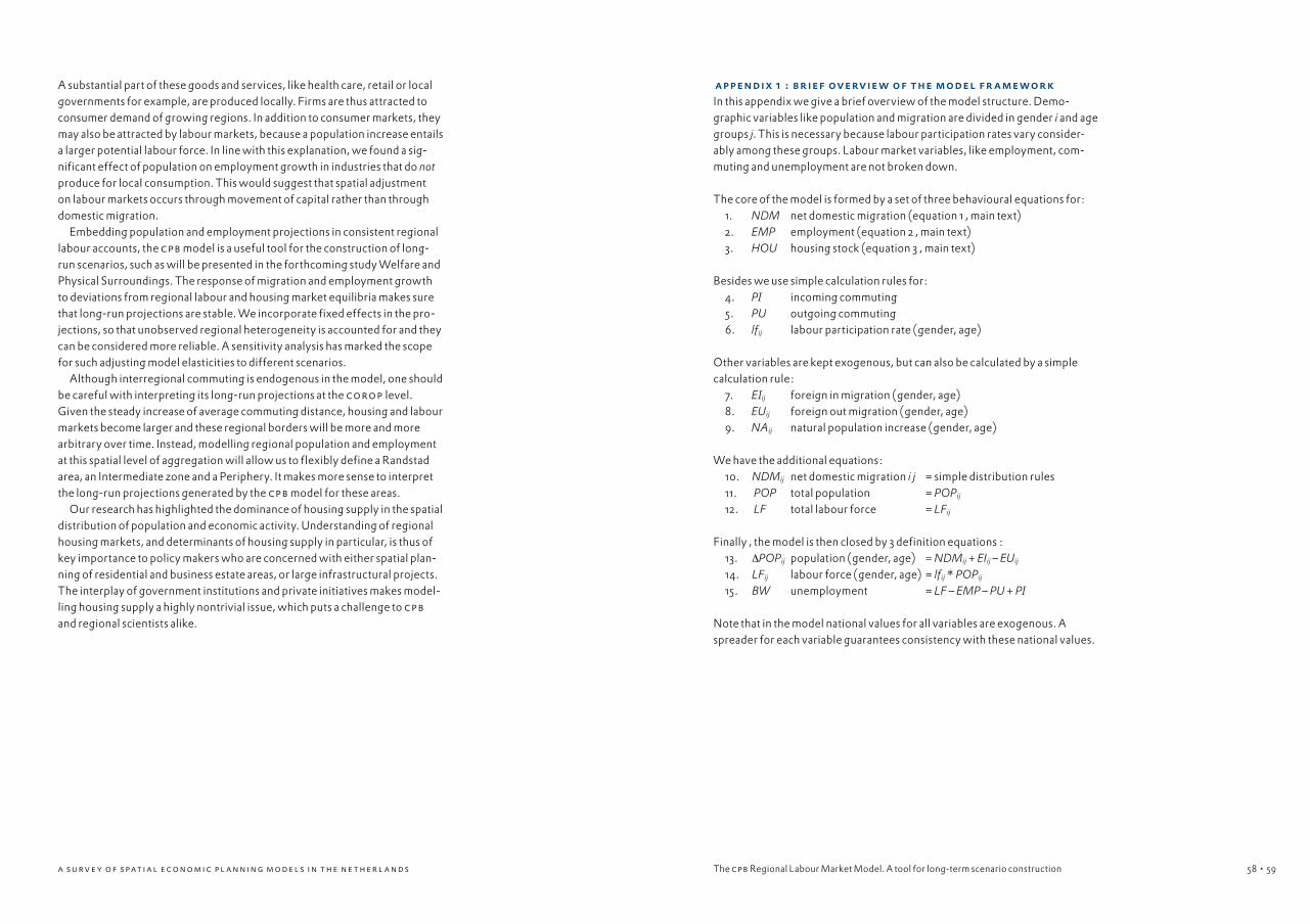
58 a s u rv e y o f s pat i a l eco n om i c p l a nni n g mo d el s i n t he ne t her l a nd s • 5958
A substantial part of these goods and services, like health care, retail or local governments for example, are produced locally. Firms are thus attracted to consumer demand of growing regions. In addition to consumer markets, they may also be attracted by labour markets, because a population increase entails a larger potential labour force. In line with this explanation, we found a sig-nificant effect of population on employment growth in industries that do not produce for local consumption. This would suggest that spatial adjustment on labour markets occurs through movement of capital rather than through domestic migration. Embedding population and employment projections in consistent regional labour accounts, the cpb model is a useful tool for the construction of long-run scenarios, such as will be presented in the forthcoming study Welfare and Physical Surroundings. The response of migration and employment growth to deviations from regional labour and housing market equilibria makes sure that long-run projections are stable. We incorporate fixed effects in the pro-jections, so that unobserved regional heterogeneity is accounted for and they can be considered more reliable. A sensitivity analysis has marked the scope for such adjusting model elasticities to different scenarios. Although interregional commuting is endogenous in the model, one should be careful with interpreting its long-run projections at the corop level. Given the steady increase of average commuting distance, housing and labour markets become larger and these regional borders will be more and more arbitrary over time. Instead, modelling regional population and employment at this spatial level of aggregation will allow us to flexibly define a Randstad area, an Intermediate zone and a Periphery. It makes more sense to interpret the long-run projections generated by the cpb model for these areas. Our research has highlighted the dominance of housing supply in the spatial distribution of population and economic activity. Understanding of regional housing markets, and determinants of housing supply in particular, is thus of key importance to policy makers who are concerned with either spatial plan-ning of residential and business estate areas, or large infrastructural projects. The interplay of government institutions and private initiatives makes model-ling housing supply a highly nontrivial issue, which puts a challenge to cpb and regional scientists alike.
appendix 1 : br ief overvie w of the model fr a me wor kIn this appendix we give a brief overview of the model structure. Demo- graphic variables like population and migration are divided in gender i and age groups j. This is necessary because labour participation rates vary consider-ably among these groups. Labour market variables, like employment, com-muting and unemployment are not broken down.
The core of the model is formed by a set of three behavioural equations for: 1. NDM net domestic migration (equation 1 , main text)2. EMP employment (equation 2 , main text)3. HOU housing stock (equation 3 , main text)
Besides we use simple calculation rules for:4. PI incoming commuting5. PU outgoing commuting6. lfij labour participation rate (gender, age)
Other variables are kept exogenous, but can also be calculated by a simple calculation rule:
7. EIij foreign in migration (gender, age)8. EUij foreign out migration (gender, age)9. NAij natural population increase (gender, age)
We have the additional equations: 10. NDMij net domestic migration i j = simple distribution rules11. POP total population = POPij
12. LF total labour force = LFij
Finally , the model is then closed by 3 definition equations :13. ΔPOPij population (gender, age) = NDMij + EIij – EUij
14. LFij labour force (gender, age) = lfij * POPij
15. BW unemployment = LF – EMP – PU + PI
Note that in the model national values for all variables are exogenous. A spreader for each variable guarantees consistency with these national values.
The cpb Regional Labour Market Model. A tool for long-term scenario construction

60 a s u rv e y o f s pat i a l eco n om i c p l a nni n g mo d el s i n t he ne t her l a nd s • 6160
appendix 2 : data sourcesSince 1970 Statistics Netherlands has produced regional sectoral data for corop regions (Eurostat nuts3 level), which are consistent with natio-nal employment and production in the National Accounts.31 In these data, employment is measured in labour years for employees only. At cpb, the sectoral employment data are converted to employment in persons. Also. regional employment for self employed has been estimated separately, both in labour years and in persons. Population data and data on migration flows are based on Municipality Administrations (gba). Municipalities can easily be added up to corop regions. The migration data include gross domestic flows between regions and foreign migration flows, distinguishing 2 gender and 7 age groups. Consequently, natural population increase can be obtained as a residual. Data on the labour force, on commuting and on unemployment are based on the Labour Force Survey (ebb) from Statistics Netherlands. This survey has been held annually since the early nineties. The survey is not automati-cally consistent with either National Accounts or gba. At cpb regional labour force and unemployment as well as commuting flows and unemployment are revised to construct consistent regional labour accounts. Finally, data on the housing stock are produced at Statistics Netherlands, they have been kindly provided to us by abf Research. All data used for our analysis can be obtained upon request.
appendix 3 : nut s 3 cl a s sific ation of the nether l ands
Randstad Intermediate Zone Periphery
17 Utrecht 13 Veluwe 1 East Groningen 31 Zeeuws Vlaanderen
18 North of North Holland 14 Achterhoek 2 Delfzijl & surroundings 32 Other Zeeland
19 Alkmaar & surroundings 15 Arnhem/Nijmegen 3 Other Groningen 37 North Limburg
20 IJmond 16 Southwest Gelderland 4 North Friesland 38 Middle Limburg
21 Haarlem agglomeration 33 West North Brabant 5 Southwest Friesland 39 South Limburg
22 Zaanstreek 34 Middle North Brabant 6 Southeast Friesland
23 Greater Amsterdam 35 Northeast North Brabant 7 North Drenthe
24 Gooi & Vechtstreek 36 Southeast North Brabant 8 Southeast Drenthe
25 Leiden & Bollenstreek 40 Flevoland 9 Southwest Drenthe
26 The Hague agglom. 10 North Overijssel
27 Delft & Westland 11 Southwest Overijssel
28 East South Holland 12 Twente
29 Greater Rijnmond
30 Southeast S. Holland
The cpb Regional Labour Market Model. A tool for long-term scenario construction
31. The regional classification
dates from early 1970 and has
undergone only a few minor revi-
sions. The Netherlands are divided
in 40 nuts3 regions, which can
be added up to the 12 Dutch pro-
vinces.
43
6 7
8
13
1
14
12
10
36
17
9
35
5
29
33
40
15
18
32
34
37
23
16
31
39
38
2
28
30
40
11
19
26
25 24
20
18
27
2122
32
4
CPB_fig3

a s u rv e y o f s pat i a l eco n om i c p l a nni n g mo d el s i n t he ne t her l a nd s
References
abf research (2002), primos Prognose-
model voor bevolking, huishoudens en
woningbehoefte, Ministry of Housing,
Spatial Planning and Environment, the
Netherlands.
Anas, A., R. Arnott, and K.A. Small
(1998), ‘Urban Spatial Structure’, Journal of
Economic Literature, 36(3): 1426–1464.
Boarnet, M. G. (1994), ‘The monocentric
model and employment location’, Journal of
Urban Economics, 36: 79–97.
Broersma, L. and J. Van Dijk (2002),
‘Regional labour market dynamics in The
Netherlands’, Papers in Regional Science:
The journal of the RSAI, 81: 343–364.
Carlino, G. A. and E.S. Mills (1987), ‘The
Determinants of County Growth’, Journal of
Regional Science, 27(1): 39–54.
cpb (1990), athena: A macrosectoral
model for the Dutch economy, cpb monogra-
fie nr. 30, The Hague: Centraal Planbureau.
Decressin, J. and A. Fatas (1995),
‘Regional labour market dynamics in
Europe’, European Economic Review, 9:
1627–1655.
Dijk, J. v., H. Folmer, H.W.J. Herzog and
A.M. Schlottmann (1989), ‘Labour market
institutions and the efficiency of interregio-
nal migration: a cross-nation comparison’,
pp. 61–83 in: J. v. Dijk,
H. Folmer, H. W. J. Herzog, and A. M.
Schlottmann (eds.), Migration and labour
market adjustment, Dordrecht: Kluwer
Academic Publishers.
Muth, R. F. (1971), ‘Migration: chicken
or egg?’, Southern Economic Journal, 37(3):
295–306.
oecd (2000), ‘Disparities in regional
labour markets’, pp.31–78 in: oecd
Employment outlook 2000.
Rietveld, P. and F.R. Bruinsma (1998),
Is infrastructure effective? Transport infra-
structure and accessibility: impacts on the
space economy, Berlin: Springer Verlag.
Steinnes, D.N.(1977), ‘Causality and
Intra urban Location’, Journal of Urban
Economics, 4: 69–79.
Steinnes, D. N. (1982), ‘Do ‘People
Follow Jobs’ or do ‘Jobs Follow People’? A
Causality Issue in Urban Economics’, Urban
Studies, 19: 187–192.
Vermeulen, W. (2003), A Model for
Dutch Commuting, cpb Report,(1), 34–43.
Vermeulen W. and J.N. van Ommeren
(2004), ‘Interaction of Regional Population
and Employment: Identifying Short-Run
and Equilibrium Adjustment Effects’,
Tinbergen Discussion Paper, ti 2004-083/3.
raem: Regional Applied
general Equilibrium Model
for the Netherlands

64
r aem: r egional applied gener al equilibr ium model for the nether l ands Mark Thissen
IntroductionAt the beginning of the 21st century tno, the University of Groningen and the Free University of Amsterdam embarked on a joint project to develop a multi-sector regional applied general equilibrium model for the Netherlands (r aem). Following two years of development the model is now finished and can be used for policy analysis. r aem is based on monopolistic competition and emphasises spatial agglo-meration, dispersion, spatial networks and market imperfections along the lines discussed in the Introduction to the book. The model is especially equip-ped to evaluate policy on transport infrastructure, although it can easily be extended to analyse the economic effects of other policies. It determines the overall effects of different policy measures and takes indirect effects into account in detail. Since September 11 2001 fear of terrorist attacks on transport infrastruc-ture has increased. The attacks on trains in Madrid in March 2004 emphasize the focus of terrorists on transport. Threats have been made against the Holland Tunnel in the United States and several tunnels in the Netherlands: the Benelux tunnel in Rotterdam, for instance, has seen increased police surveillance on several occasions. Although the terrorists’ objective may be to achieve the maximum number of casualties, attacks of this kind have direct and indirect economic effects. The additional costs of transport and commuting due to such attacks invol-ve not only the direct effect of a damaged transport infrastructure but also those of increased security measures, which can be substantial and should therefore be taken into account. The major changes in the whole organiza-tion and security of us air travel have resulted in large increases in the cost to travellers (in terms of both travel time and money), and these additional costs have economic effects. As a first case to present the r aem model we determine the economic effects of such an attack, focusing solely on those due to the spatial distur-bance introduced by the attack and abstracting from the direct damage due to the explosion, casualties and possible psychological damage.1 We also assume at the outset that the transport link will not be rebuilt, as the cost of rebuilding and the temporary spatial distortion are likely to be smaller than the long-term effects of not rebuilding, which are factored in here. The analysis is therefore only for illustrative purposes. The link chosen in the experiment is the Van Brienenoord bridge in Rotterdam: unlike with a bridge, it is difficult to ima-gine an attack that could result in permanent damage to a tunnel.
r aem: Regional Applied general Equilibrium Model for the Netherlands
1. We follow the methodology
described in Thissen(2004b).
• 65

66 a s u rv e y o f s pat i a l eco n om i c p l a nni n g mo d el s i n t he ne t her l a nd s • 6766
The modelThe model fits in with the new economic geography theory (neg) as described in the Introduction to the book and builds on models developed by Venables (1996) and Oosterhaven et al. (2001). Markets operate under conditions of monopolistic competition, with perfect competition as a special case. The choice between monopolistic and perfect competition is based on data on production and trade in the Netherlands and is not made a priori. The estimated degree of competition on the different product markets deter-mines the agglomeration strength of the respective sectors, in other words the degree to which a particular sector benefits from having other firms in its neighbourhood. The equations referred to in the text below are given in Appendix 1.
Although most recent models used in policy analysis resort to simplifying the theoretical models to make them analytically tractable (see Baldwin et al. 2003 for an overview), r aem does not use these empirical shortcuts and is therefore a theoretically sound and complete model, built in the tradition of general equilibrium models. The main reason for not using simplifications that would simplify the development of the model and analysis using it is the effect that these could have on policy evaluation. The model identifies all five spatial interactions characteristic of neg models, as discussed in the Introduction to the book. Trade costs, commuting costs and the regional availability of land and housing determine the relative strength of these forces and thus the economic shape of the country. Figure 1 gives an overview of the model from the perspective of infrastruc-ture projects. In the figure, changes in transport costs trickle down through the economy, affecting regional (as well as national) economic development. Transport costs affect the labour market via commuting and the possibility of migration (the housing effect and cost-of-living effect), they affect prices directly and affect logistical costs and labour costs (e.g. with respect to sales-men) that influence the production process. The interaction between regio-nal labour supply and demand and wages results in both national and regional changes in vacancies and unemployment. Changes in regional production affect intermediate demand, consumption and variety through the variety effect, the market-access effect and the market-crowding effect. This, then, is a brief description of the main effects operating in r aem.
General structure of the modelThe model uses a multi-sector approach, identifying fourteen sectors in the standard sbi ’93 classification. In line with the theoretical framework in the neg literature, a number of varieties are produced in each sector identified. All these varieties are imperfect substitutes. The model identifies 40 regions in the Dutch corop classification. Transport costs link the regional goods markets. An substantial proportion of the indirect effects of transport infrastructure on the regional economy occur through agglomeration effects. If a firm is able
to choose between several varieties of imports, it can increase productivity by having a more roundabout production process. At the same time the utility to consumers increases if they have more variety to choose from, producing strong agglomeration effects in regions. If products become more expensive owing to increased transport costs, access to variety decreases: thus produc-tivity declines exponentially with a decline in the scale of operating. The labour market is based on the Pissarides (2000) approach, incorpo-rating search theory. The unemployed search for jobs in the various regions with a typical search intensity, while firms look for employees and set a num-ber of vacancies. Given the probability of a match, an unemployed person is hired. In the long run, equilibrium labour supply is such that utility is equal for workers among regions, taking local differences such as those in house prices into account. The medium-term version of the model limits migration between regions and therefore leaves open the possibility of regional utility differences.
Production and agglomerationMonopolistic competition is modelled using a nested production function, as in Venables (1996). The first step is to determine what the sectoral demand for goods will be, using a standard Cobb-Douglas production function (1). The second step is to specify regional demand, using a standard Dixit-Stiglitz ces approach (4).
r aem: Regional Applied general Equilibrium Model for the Netherlands
g
h
f
Infrastructure project
Transport costs
Migration
Commuting Logistical costs Labour costs
Prices
g g g
g
g
gRegional labour
supply
Production
Intermediate
demand
Consumption
g g
h
f
iRegional wage f
f
Regional vacancies
and unemployment
i
i
h
Regional
number of
companies
(varieties)
i
h
hg
i
Regional labour
demand
Figure 1. The effect of infrastructure projects in r aem
g
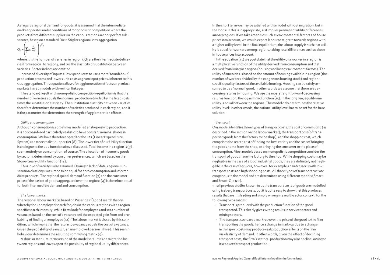
68 a s u rv e y o f s pat i a l eco n om i c p l a nni n g mo d el s i n t he ne t her l a nd s • 6968
As regards regional demand for goods, it is assumed that the intermediate market operates under conditions of monopolistic competition where the products from different suppliers in the various regions are not perfect sub-stitutes, based on a standard Dixit-Stiglitz regional ces aggregation Qj = Σ
ini Qij
where ni is the number of varieties in region i, Qij are the intermediate delive-ries from region i to region j, and σ is the elasticity of substitution between varieties. Sector indices are omitted. Increased diversity of inputs allows producers to use a more ‘roundabout’ production process and lowers unit costs at given input prices, inherent to this ces aggregation. This equation allows for agglomeration effects on product markets in neg models with vertical linkages. The standard result with monopolistic competition equilibrium is that the number of varieties equals the nominal production divided by the fixed costs times the substitution elasticity. The substitution elasticity between varieties therefore determines the number of varieties produced in each region, and it is the parameter that determines the strength of agglomeration effects.
Utility and consumptionAlthough consumption is sometimes modelled analogously to production, it is not considered particularly realistic to have constant nominal shares in consumption. We have therefore opted for the les (Linear Expenditure System) as a more realistic upper tier (6). The lower tier of our Utility function is analogue to the ces function above discussed. Total income in a region is (7) spent entirely on consumption, of course. The allocation of income to goods by sector is determined by consumer preferences, which are based on the Stone-Geary utility function (14). Thus love of variety is also assumed. Owing to lack of data, regional sub-stitution elasticity is assumed to be equal for both consumption and interme-diate products. The regional spatial demand function (7) and the consumer price of the basket of goods aggregated over the regions (4) is therefore equal for both intermediate demand and consumption.
The labour marketThe regional labour market is based on Pissarides’ (2000) search theory, whereby the unemployed search for jobs in the various regions with a region-specific search intensity, while firms look for employees and set a number of vacancies based on the cost of a vacancy and the expected gain from and pro-bability of finding an employee (12). The labour market is closed by this con-dition, which means that the return to a vacancy equals the cost of a vacancy. Given the probability of a match, an unemployed person is hired. This search behaviour determines the resulting commuting matrix (9). A short or medium-term version of the model sets limits on migration be- tween regions and leaves open the possibility of regional utility differences.
In the short term we may be satisfied with a model without migration, but in the long run this is inappropriate, as it implies permanent utility differences among regions. If we take amenities such as environmental factors and house prices into account, we would expect labour to migrate towards regions with a higher utility level. In the final equilibrium, the labour supply is such that util-ity is equal for workers among regions, taking local differences such as those in house prices into account. In the equation (13) we postulate that the utility of a worker in a region is a multiplicative function of the utility derived from consumption and that derived from living in a region (housing and living environment factors). The utility of amenities is based on the amount of housing available in a region (the number of workers divided by the exogenous housing stock) and region- specific quality factors of the available housing. Housing can be safely as-sumed to be a ‘normal’ good, in other words we assume that there are de-creasing returns to housing. We use the most straightforward decreasing returns function, the logarithmic function (15). In the long run, equilibrium utility is equal between the regions. The model only determines the relative utility level: in other words, the national utility level has to be set for the base solution.
TransportOur model identifies three types of transport costs, the cost of commuting (as described in the section on the labour market), the transport cost (of trans-porting goods from the factory to the shop), and the shopping cost, which comprises the search cost of finding the best variety and the cost of bringing the goods home from the shop, or bringing the consumer to the place of consumption. Most models based on monopolistic competition consider the transport of goods from the factory to the shop. While shopping costs may be negligible in the case of a lot of industrial goods, they are definitely not negli-gible in the case of services, however: for example a hairdresser’s with low transport costs and high shopping costs. All three types of transport cost are exogenous to the model and are determined using different models (Smart and Smart-G, tno).1In all previous studies known to us the transport costs of goods are modelled using iceberg transport costs, but it is quite easy to show that this produces results that are misleading and simply wrong in a multi-sector context, for the following two reasons:
· Transport is produced with the production function of the good transported. This clearly gives wrong results in service sectors and mining sectors.
· The transport costs are a mark-up over the price of the good to the firm transporting the goods, hence a change in mark-up due to a change in transport costs may produce real production effects on the firm via elasticity of demand. In other words, given the effect of declining transport costs, the firm’s sectoral production may also decline, owing to its reduced transport production.
r aem: Regional Applied General Equilibrium Model for the Netherlands
⎛ ⎞⎜ ⎟⎝ ⎠
σ –1σ
σσ –1

70 a s u rv e y o f s pat i a l eco n om i c p l a nni n g mo d el s i n t he ne t her l a nd s • 7170
We therefore use a different approach to modelling transport costs. In r aem, transport costs are a mark-up over the price in a competitive transport mar-ket where there is one price for transport. This price is set as the numerair in the model. Thus by setting the mark-up of transport costs over the price, we immediately set the real transport production. We can now determine the total transport used in the model: this equals the total nominal value of trans-ported goods times the mark-up (17). We also assume that the demand for transport goods is spread over the country regionally, based on the historical situation (18), as there is little empirical evidence of any relationship between transport production and the location of either transport production or trans-port consumption. Transport is produced using a production function compa-rable to the other sectors in the model. r aem distinguishes between shopping costs and transport costs, shopping costs typically being non-monetary costs,2 i.e. they are produced and con-sumed by the household, not by the transport sector. These shopping costs affect regional demand for certain goods, however, so they are included in the mark-up over the price of goods with respect to spatial demand, but omit-ted with respect to material balances.
The governmentThe role of the government in the model is merely redistributive. It raises income tax to pay for unemployment benefit, which is set at a percentage of the average wage in the Netherlands. Assuming that the government bal-ances its budget, we also know the income tax rate (21).
Interpreting the model: the main interactionsThe product markets and the labour market are the crucial markets when it comes to the role of transport infrastructure in the economy. The product markets are affected by changes in transport infrastructure via regional trade, and the labour market via workers’ commuting behaviour. The effects of a change in transport costs on product markets are along the lines outlined in the Introduction to the book. We therefore simply refer the reader there and continue discussing the effects of the labour market in r aem.
Effects on the labour marketA sudden increase in transport costs will have strong repercussions on the economy via the regional labour market. Pissarides’ (2000) approach to modelling the labour market assumes that the unemployed search for jobs in the various regions with a typical search intensity, while firms look for employees and set a number of vacancies. Given the probability of a match, an unemployed person is hired. This search behaviour determines the resul-ting commuting matrix. The model incorporates unemployment in different regions due to mismatch between searching employees and employers. The labour supply is determined by the long-term equality of the utility of workers among regions, taking local differences such as those in house prices into account. This price of space, determined by the housing stock and the number of people in a region, gives us the equilibrium solution.3
How an increase in transport costs due to a terrorist attack affects the eco-nomy is graphically depicted in Figure 2, where product markets are taken ceteris paribus. Transport costs affect the economy by influencing economic behaviour with regard to migration and commuting. A terrorist attack on transport infrastructure in a particular region will cause a rise in all the transport costs to that region, inducing some people to stop looking for jobs in that region and thus reducing the local labour supply. This will cause a decline in the region’s production, leading in turn to lower productivity through agglomeration effects and reducing the relative wage level there. The lower relative wage level causes emigration out of the region, reducing the supply of labour even more. The opposite effect can also occur, however: people living in the region where the terrorist attack took place will stop looking for jobs outside it as transport costs increase. Whether the local supply of labour will increase or decrease depends on the relative flow of incoming commuter traffic (into the region) vis-à-vis outgoing commuter traffic (out of the region).4
Higher transport costs will also have an effect on migration, hence on the labour market and the regional economy. Here too, however, what direction the effect will take is not clear beforehand. Two opposite effects can occur, depending on the size (or economic mass) of the region. If we are in the middle of a conurbation with strong economic activity we can expect people to migrate there because the higher transport costs make commuting to it less attractive. If we have a region with little economic activity we can expect
r aem: Regional Applied general Equilibrium Model for the Netherlands
2. For the sake of convenience we
assume that the shopping costs
of the firm are also internal to the
firm. In the case of firms, cf. in par-
ticular the search costs and travel
costs involved in making business
deals.
4. This deviates from the standard
Krugman (1980) monopolistic
competition model, where there
are many possible equilibriums.
5. Both flows should be weighted
with the transport costs to com-
muters
Higher relative wage
gHigher labour supply
Lower transport costs
gLower labour supply
Lower relative wage
i
f
gMigration
Migration
f
i Scale & scope effectsg
Lower local production
i
Regional trade effectg
Higher local production
i
Scale & scope effects
f
f
h
hDistributive effects
Generative effects
i
g
iCommuting
Migration
Figure 2. Effects of changes in transport costs on labour markets

72 a s u rv e y o f s pat i a l eco n om i c p l a nni n g mo d el s i n t he ne t her l a nd s • 7372
people to migrate out of it because commuting costs increase for people there. Figure 2 assumes that the effect of immigration into the region is domi-nant. Again the effect is heightened by increases in production and associated scale and scope effects.
Applicationsr aem has been used to answer a number of policy questions since 2000, analysing the effects of: a new rail link between the Randstad area and the North of the Netherlands; a rail link between the main conurbations in the Randstad5; a reduction in through traffic;6 speed limits on trunk roads around Rotterdam; and road pricing. In addition to these actual applications during the past few years, the model has a broad spectrum of potential research questions that it can answer. It can be used for both impact and forecast analysis. It cannot be used to determine a time path towards a long-term equilibrium, however, as it is based on compar-ative statics.7
r aem is a multipurpose model that can be used (with some adjustments) to answer many regional policy questions. Two types of analysis, impact analysis and prognosis, are possible. The model can be used not only to analyse the future spatial economic effects of policy measures and investment decisions but also to give a prognosis of the spatial distribution of future economic growth (scenario analysis). Table 1 gives an overview of the different policy measures that can be analysed using r aem (the list is not exhaustive, how-ever).Many types of impact analysis can be carried out using the model. It was developed to analyse the effects of both point and line infrastructure, but it can also be used for other policy measures, for example changes in the railway timetable, road pricing or different plans for the spatial distribution of hous-ing. In addition to impact analysis, the model can be used to forecast spatial economic development in the Netherlands. It is not particularly well equip-ped for short-term scenarios, having been specially designed to deal with long-term spatial economic scenarios. It can be used to regionalize the cpb’s macro-economic forecasting, infrastructure scenarios (nvvp) or scenarios for the regional distribution of housing. It can also be used to estimate trade flows between regions, e.g. aggregated IO tables, as well as forecasting the economic outcomes of different scenarios, as already mentioned.
Case studyIn this case study we analyse the economic effects of a terrorist attack result-ing in an increase in transport costs. These costs can increase as a result of damage to and/or reorganization of infrastructure. Hence not only a direct attack on transport infrastructure, such as the attack in Madrid in 2004, but also the New York attack in 2001 induced a significant rise in transport costs, owing to the security measures that had to be taken. The hypothesis is that
Table 1. Possible applications of r aem
impact
Effects of changes in generalized transport costs due to:
Infrastructure link: road, river, rail, passengers, freight
Timetables: passengers, freight
Infrastructure node: capacity
Infrastructure node: capacity
Road pricing
prognosis
Spatial economic development scenarios:
Regionalization of national scenarios (cpb and nv vp)
Estimating IO tables
Spatial planning: spatial allocation of housing
Spatial welfare: social security
the changes in transport costs due to a terrorist attack are significant and have significant negative economic effects. A simulation analysis was carried out to estimate the magnitude of the economic effect of a possible terrorist attack on the Van Brienenoord bridge in the Netherlands. r aem was used to estimate these economic effects. Using r aem has the advantage of not overestimating effects as linear IO models do, it can also take agglomeration effects and non-perfect competition into account, and it is strongly based on the recent theory of the New Economic Geography.
Analysing the economic effects of a terrorist attack on transport infrastructureIt would seem that we know the maximum effect beforehand: this is simply the cost of rebuilding the destroyed infrastructure and the temporary effect of misallocation of resources during the period that the infrastructure remains damaged. The economic costs may be much higher, however, if transport costs rise permanently, owing to increased security measures and reorganiza-tion of the transport system. Another possibility is not to rebuild the damaged transport link. This would be the best option if the economic cost of not having the link were to be less than the cost of repairing it. In this case, as in the case of a general increase in costs as described above, a more extensive study of the economic effects of a terrorist attack on transport infrastructure is needed.
Transport costs Figure 1 showed how changes in transport costs due to ter-rorist attacks on infrastructure can affect the economy. Changes in these costs directly affect consumption and production decisions via their effect on prices, while at the same time having strong effects on the labour market via commuting and migration behaviour.
r aem: Regional Applied general Equilibrium Model for the Netherlands
.
5. It should be noted that an earlier
version of the model was used for
the first two projects.
6. The model was evaluated as
good in a second opinion by seo
for a project on the effect of redu-
cing through traffic.
7. Policy-makers naturally prefer a
time path towards the final equili-
brium, but this, unfortunately, is a
hazardous theoretical path for an
economic modeller.
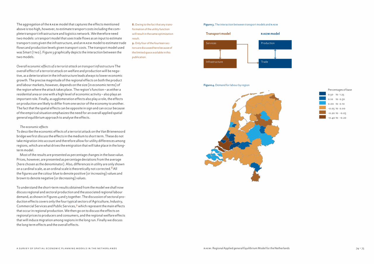
74 a s u rv e y o f s pat i a l eco n om i c p l a nni n g mo d el s i n t he ne t her l a nd s • 7574
The aggregation of the r aem model that captures the effects mentioned above is too high, however, to estimate transport costs including the com-plete transport infrastructure and logistics network. We therefore need two models: a transport model that uses trade flows as an input to estimate transport costs given the infrastructure, and an r aem model to estimate trade flows and production levels given transport costs. The transport model used was Smart (tno). Figure 3 graphically depicts the interaction between the two models.
Overall economic effects of a terrorist attack on transport infrastructure The overall effect of a terrorist attack on welfare and production will be nega-tive, as a deterioration in the infrastructure leads always to lower economic growth. The precise magnitude of the regional effects on both the product and labour markets, however, depends on the size (in economic terms) of the region where the attack takes place. The region’s function – as either a residential area or one with a high level of economic activity – also plays an important role. Finally, as agglomeration effects also play a role, the effects on production are likely to differ from one sector of the economy to another. The fact that the spatial effects can be opposite in sign and can occur because of the empirical situation emphasizes the need for an overall applied spatial general equilibrium approach to analyse the effects.
The economic effectsTo describe the economic effects of a terrorist attack on the Van Brienenoord bridge we first discuss the effects in the medium to short term. These do not take migration into account and therefore allow for utility differences among regions, which are what drives the emigration that will take place in the long-term model. Most of the results are presented as percentage changes in the base value. Prices, however, are presented as percentage deviations from the average (here chosen as the denominator). Also, differences in utility are only shown on a cardinal scale, as an ordinal scale is theoretically not corrected.8 All the figures use the colour blue to denote positive (or increasing) values and brown to denote negative (or decreasing) values.
To understand the short-term results obtained from the model we shall now discuss regional and sectoral production and the associated regional labour demand, as shown in Figures 4 and 5 together. The discussion of sectoral pro-duction effects covers only the four typical sectors of Agriculture, Industry, Commercial Services and Public Services,9 which represent the main effects that occur in regional production. We then go on to discuss the effects on regional prices to producers and consumers, and the regional welfare effects that will induce migration among regions in the long run. Finally we discuss the long term effects and the overall effects.
r aem: Regional Applied general Equilibrium Model for the Netherlands
Services
i
Infrastructureg
Production
i
Tradeg
f
Transport model r aem model
Figure 3. The interaction between transport models and r aem
Figure 4. Demand for labour by region
8. Owing to the fact that any trans-
formation of the utility function
will result in the same optimization
result.
9. Only four of the fourteen sec-
tors are discussed here because of
the limited space available in this
publication.
Percentages of base
0.50 to 1.25
0.10 to 0.50
0.00 to 0.10
-0.05 to 0.00
-0.20 to -0.05
-0.40 to -0.20

76 a s u rv e y o f s pat i a l eco n om i c p l a nni n g mo d el s i n t he ne t her l a nd s • 7776
Short term effects on production and the labour market As Figures 4 and 5 show, the effects are strongest in the regions around the bridge. The Greater Rotterdam region, where the bridge is located, however, reacts completely differently to its disappearance than the regions to the east of the bridge. The main reason for this is the large internal market in the Greater Rotterdam region, the production structure in the various regions, and the relatively small effect in terms of additional transport costs of the terrorist attack in Greater Rotterdam itself. These relatively small effects in Greater Rotterdam are due to the shift of traffic that used to transit Rotterdam via the Van Brienenoord bridge and now uses links to the east, causing increased con-gestion in those areas and leaving the roads in Rotterdam itself (apart from the links between the two sides of the river) relatively empty. The large internal market and the relatively small increase in transport costs (especially internally) for the Greater Rotterdam region result in a relative competitive advantage in industrial goods. The associated shift from the labour-intensive service sector towards the labour-extensive industrial sector results in an increase in production (at constant prices) and a reduction in labour demand. The reduced supply of labour (for the whole area around the bridge) because of fewer ‘in-commuters’ also plays a role in pushing up wages in the region and thereby reducing labour demand. The effects on labour supply and demand add up to a decline in unemployment in this area (see Figure 6). The effects are quite different in the regions to the east of the bridge: trans-port and commuting costs rise the most, causing labour supply to increase owing to reduced out-migration and reducing these regions’ relative com-petitiveness. The loss in relative competitiveness in the service sector is smal-lest with regard to exports10 and largest with regard to imports.11 These regions therefore see a shift out of the industrial sector into the (relatively labour-intensive) service sector, resulting in an overall decline in production but an increase in labour demand. We are left with the two regions of Delft and The Hague, which need to be discussed separately, as they are located next to each other but react com-pletely differently to the increase in transport costs. Delft seems to benefit from the reduction in the usage of the motorway to Rotterdam and The Hague, increasing its access to these large economic markets. Industrial pro-duction thus increases in this region, with increased labour demand and redu-ced unemployment. The increase in transport costs to other regions, howev-er, induces people to demand the relatively unproductive services from their own region, reducing its overall productivity (this makes Delft different from Greater Rotterdam). The Hague region is mainly a service economy (includ-ing the seat of government) with a relatively high percentage of services exported to other regions. The reduced demand for the export of services from The Hague to other cities due to the increase in transport costs results in a reduction in service sector production and a loss of productivity (a negative agglomeration effect12), inducing both a reduction in labour demand and an increase in unemployment.
r aem: Regional Applied general Equilibrium Model for the Netherlands
total production
1: 0.20 - 1.00
2: 0.10 - 0.20
3: 0.00 - 0.10
4: -0.25 - 0.00
5: -1.00 - -0.25
6: -1.25 - -1.00
sector production
7: agriculture
8: industry
9: commercial services
10 : public services
Figure 5. Production in constant prices by region
Figure 6. Changes in the unemployment rate
10. As the change in competitive-
ness is relatively small in the case
of services such as hairdressing,
which are typically produced at the
place of consumption.
11. Note that the model does not
include foreign countries, so the
terms ‘imports’ and ‘exports’
apply exclusively to trade between
the Dutch corop regions.
12. It could be argued that the
location of government is institu-
tionally determined and therefore
not affected by changes in trans-
port costs. The model does not
take these institutional effects
into account, so it may be that the
effects on The Hague are slightly
exaggerated.
Constant prices and
percentages of base
0.20 t0 1.00
0.10 to 0.20
0.00 to 0.10
-0.25 to 0.00
-1.00 to -0.25
-1.25 to -1.00
Sector production
Agriculture
Industry
Commercial services
Public services
Percentages of base
0.03 t0 0.05
0.01 to 0.03
0.00 to 0.10
-0.01 to 0.00
-0.05 to -0.01
-0.15 to -0.05

78 a s u rv e y o f s pat i a l eco n om i c p l a nni n g mo d el s i n t he ne t her l a nd s • 7978
The other regions of the Netherlands seem to benefit from their increased competitive advantage only in the form of a relative increase in their prices, not an increase in production. To a large extent this is due to the fact that over-all production in the Netherlands is limited by the total supply of labour, while the increased demand for transport production and the increased friction on the labour market because of increased commuting costs leave little room for an increase in production. The changes in unemployment shown in Figure 6 are expected to be a mirror image of the demand for labour. The differences are due to changes in commuting, hence the regional supply of labour. The Greater Rotterdam region is the most surprising here, with the reduced demand for labour more than offset by the willingness of workers to commute to this region.13
Short term effects on prices Markets are cleared by prices and Figures 7 and 8, showing the regional differences in producer and consumer prices, contain a lot of information on the processes at work to find a new long-term equilibri-um.14 The producer prices show the shock that is administered to the pro-ducing sectors. The loss in the regions’ competitiveness due to the increased transport cost mark-up is almost completely offset by a reduction in producer prices as industries try to defend their share of the market. The large market of Greater Rotterdam benefits from the decrease in production prices, as products for the local markets are little affected by rising transport costs. This is certainly not the case with the regions to the east of Greater Rotterdam, where the share of the local market is relatively small, resulting in a sharp increase in prices for the large amounts of imported goods. The importance of consumer transport costs (consumed and produced by consumers) also becomes clear, from the difference between producer and consumer prices. Where consumer transport costs increase (as is the case to the east of Greater Rotterdam), goods from all regions are affected, so there is no regional terms-of-trade loss, though these additional costs show up in consumer prices and do affect regional welfare.
Short term effects on welfare The regional welfare effects are a combination of the changes in income earned in the regions, commuting, employment and consumer prices. The effects, as shown in Figure 9, are not surprising, considering our previous discussion of the effects that result in regional wel-fare changes. The whole of the Netherlands is worse off. Only two regions experience a slightly positive effect, owing to a terms-of-trade effect, but these effects are very small. The negative effects are strongest to the east of Rotterdam, where congestion is greatest and the economy is highly depend-ent on Rotterdam.
Long-term effects In the long run the model also takes migration into account. The effects on prices and production are mitigated mainly by the fact that people can migrate and escape the adverse effect of the increase in transport costs. The effects on prices and the product and labour markets are therefore similar, though smaller, so these are not shown.
r aem: Regional Applied general Equilibrium Model for the Netherlands
13. Note that this is net commuting.
14. When discussing the figures
it is important to bear in mind that
a large proportion of production
consists of services, not only indu-
strial goods, and services are par-
ticularly likely to be produced and
consumed in the same region.
Figure 7. Relative producer price
Figure 8. Relative consumer price
Percentages of average
0.20 t0 0.40
0.05 to 0.20
0.00 to 0.05
-0.05 to 0.00
-0.15 to -0.05
-0.40 to -0.15
Percentages of average
0.05 t0 0.10
0.02 to 0.05
0.00 to 0.02
-0.05 to 0.00
-0.20 to -0.05
-0.40 to -0.20

80 a s u rv e y o f s pat i a l eco n om i c p l a nni n g mo d el s i n t he ne t her l a nd s • 8180
The migration flows, as shown in Figure 10, follow a pattern similar to that of the welfare effects, as set out above. It is clear, however, that everyone does not migrate to the same regions (the two with a positive welfare effect), as these cannot absorb such large numbers of people. Instead, people leaving the worst affected areas spread out over the rest of the country.
The overall effects Finally we discuss the overall effect and attempt to ans-wer the question of whether or not the bridge should be rebuilt. Owing to limitations of space we do not give a fully fledged cost-benefit analysis here; instead, we confine ourselves to a simple analysis, comparing the cost of the bridge to the change in production.15 We have chosen total value added as the best indicator of the additional ‘income earned’ due to the Van Brienenoord bridge. The overall effect of its destruction is a decline in total value added of 0.045 percent. This may look like a small amount, but it still equates to 190 million euros in 2003. We estimate the cost of building a new Van Brienenoord bridge in 2003 at 350 million euros.16 Given the pay-back time, the best policy would obviously be to rebuild it as soon as possible. This should come as no surprise, as the infra-structure around it is already available and the large regional economy around the Greater Rotterdam area has taken shape based on that infrastructure.
Discussion of the Effects Producer prices are important in explaining the economic effects of the destruction of the bridge. Competition among the regions forces firms to offset their loss of competitiveness due to higher transport costs, which they do by reducing prices. The change in producer prices is therefore a mirror image of the change in transport costs. The area most affected lies to the east of the destroyed bridge. Congestion is severe in this region, as this is where the alternative routes (and bridges) for commuters between the north and the south of the South-West of the Netherlands are situated. It is in this area, therefore, that the negative welfare effects are greatest. To understand the effects on the labour markets we also need to take sec-toral production and commuting behaviour into account. Commuting deter-mines the actual labour supply in each region and the scope for production there. It is the region’s sectoral competitiveness, however, that determines the level of wages paid and the labour demanded. If the comparative advan-tage of a region shifts to labour-intensive industries, then, it can happen (as we observed) that total regional production declines while labour demand increases. This also has an effect on the unemployment rates in each region, which, owing to commuting, are averages of the effects in the neighbouring regions.
ConclusionsThis chapter has discussed a multi-sector applied regional general equilibrium model for the Netherlands (r aem). r aem emphasises spatial agglomeration, dispersion, spatial networks and market imperfections, thereby addressing spatial economics along the lines developed in the new economic geography
15. Note that we consider a ‘pure’
production effect, only taking the
effect of the changes in consumer,
producer and worker behaviour
into account; we do not monetize
other effects such as the value of
the total increase in travel time in
terms of the value of consumers’
time.
16. We base the cost of rebuilding
the bridge on the actual cost of
constructing the second half of
it at the beginning of the 1990s,
about 250 million euros according
to the annual report of the Dutch
Ministry of Transport (mit 1993).
This, however, was only for half of
the bridge and included additional
access roads. Assuming that the
actual cost of the half of the bridge
was 125 million, and allowing for
an inflation rate of 3 percent, we
arrive a total cost of rebuilding the
bridge of 350 million euros in 2003.
r aem: Regional Applied general Equilibrium Model for the Netherlands
Figure 9. Short term effects on changes in welfare
Figure 10. Changes in population
Percentages of base
0.002 t0 0.005
0.001 to 0.002
0.000 to 0.001
-0.010 to 0.00
-0.020 to -0.010
-0.030 to -0.020
Most positive
More positive
Positive
Negative
More negative
Most negative
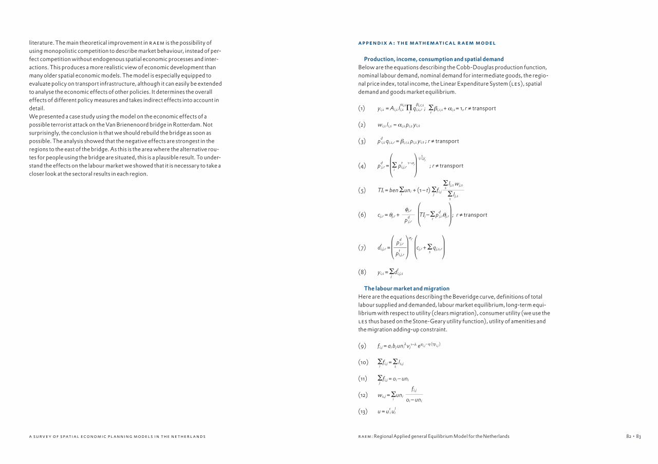
82 a s u rv e y o f s pat i a l eco n om i c p l a nni n g mo d el s i n t he ne t her l a nd s • 8382
literature. The main theoretical improvement in r aem is the possibility of using monopolistic competition to describe market behaviour, instead of per-fect competition without endogenous spatial economic processes and inter-actions. This produces a more realistic view of economic development than many older spatial economic models. The model is especially equipped to evaluate policy on transport infrastructure, although it can easily be extended to analyse the economic effects of other policies. It determines the overall effects of different policy measures and takes indirect effects into account in detail.We presented a case study using the model on the economic effects of a possible terrorist attack on the Van Brienenoord bridge in Rotterdam. Not surprisingly, the conclusion is that we should rebuild the bridge as soon as possible. The analysis showed that the negative effects are strongest in the regions to the east of the bridge. As this is the area where the alternative rou-tes for people using the bridge are situated, this is a plausible result. To under-stand the effects on the labour market we showed that it is necessary to take a closer look at the sectoral results in each region.
appendix a : the m athem atic al r aem model
Production, income, consumption and spatial demandBelow are the equations describing the Cobb-Douglas production function, nominal labour demand, nominal demand for intermediate goods, the regio-nal price index, total income, the Linear Expenditure System (les), spatial demand and goods market equilibrium.
(1) yi,s = Ai,s Ii,s Πr
qi,s,r ; Σr
βi,r,s + αi,s = 1, r ≠ transport (2) wi,s li,s = αi,s pi,s yi,s
(3) pdi,s qi,s,r = βi,r,s pi,s yi,s ; r ≠ transport
(4) pdj,r = Σ
i pt
i,j,r ; r ≠ transport
(5) TIi = ben Σi
uni + (1 – t) Σj
fi,j
(6) cj,r = θj,r + TIj – Σr
pdj,rθj,r ; r ≠ transport
(7) dti,j,r = cj,r + Σ
sqj,s,r
(8) yi,s = Σj
dti,j,s
The labour market and migration
Here are the equations describing the Beveridge curve, definitions of total labour supplied and demanded, labour market equilibrium, long-term equi-librium with respect to utility (clears migration), consumer utility (we use the les thus based on the Stone-Geary utility function), utility of amenities and the migration adding-up constraint.
(9) fi,j = ai bj uni vj e
(10) Σi
fi,j = Σs
ls,j
(11) Σj
fi,j = oi – uni
(12) ws,j = Σi
uni
(13) u = uci u
li
αi,s
⎛ ⎞⎜ ⎟⎝ ⎠
1–σr
11–σr
βi,r,s
Σs
lj,s wj,s
Σs
lj,s
φj,r
pdj,r
⎛ ⎞⎜ ⎟ ⎝ ⎠
pdj,r
pti,j,r
⎛ ⎞⎜ ⎟ ⎝ ⎠
σr ⎛ ⎞⎜ ⎟ ⎝ ⎠
1–λ ϕi,j –η (tpi,j )λ
r aem: Regional Applied general Equilibrium Model for the Netherlands
fi,j
oi – uni
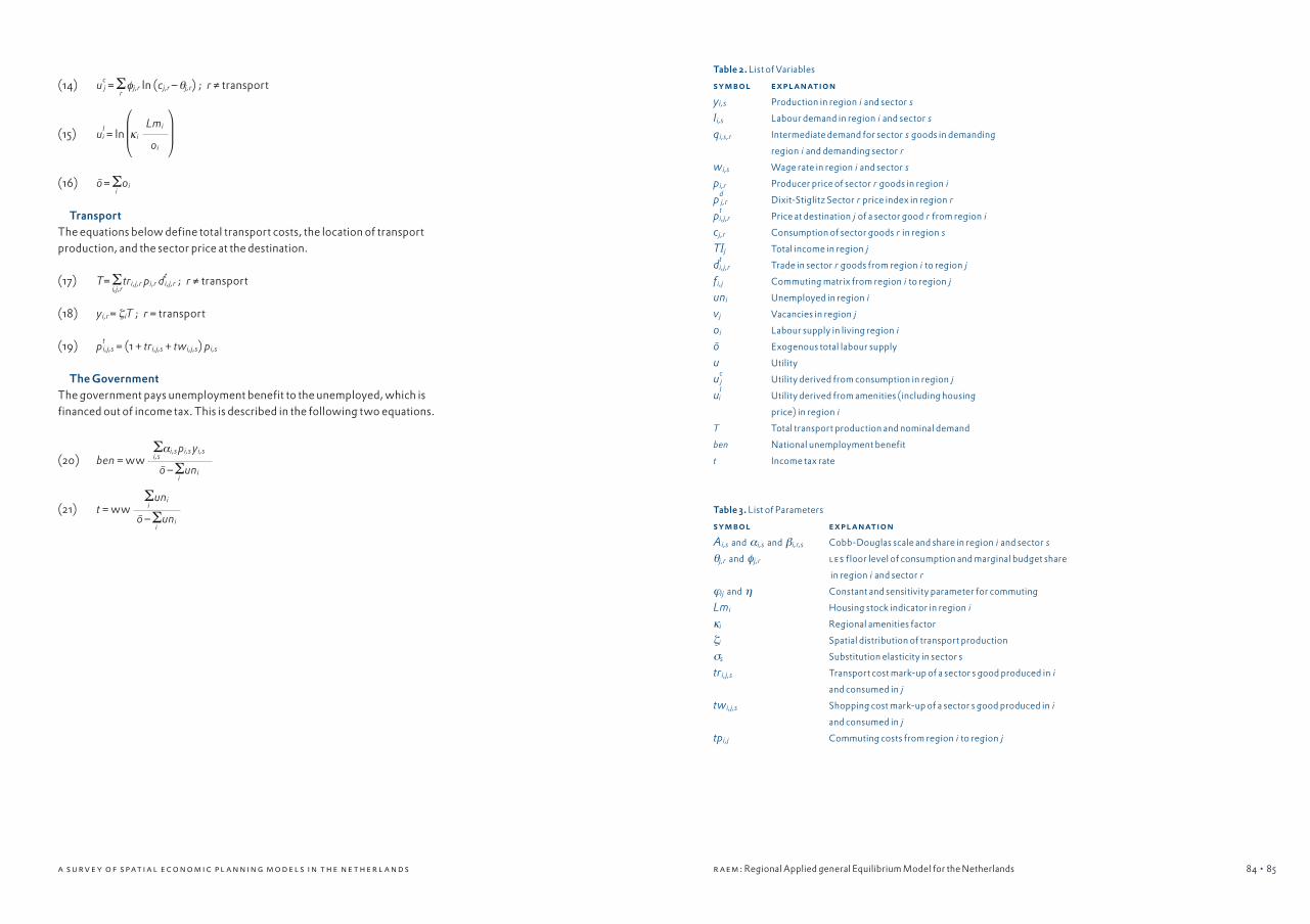
84 a s u rv e y o f s pat i a l eco n om i c p l a nni n g mo d el s i n t he ne t her l a nd s • 8584
(14) ucj = Σ
rφj,r ln (cj,r – θj,r) ; r ≠ transport
(15) uli = ln κi
(16) ō= Σi
oi
TransportThe equations below define total transport costs, the location of transport production, and the sector price at the destination.
(17) T= Σi,j,r
tri,j,r pi,r dti,j,r ; r ≠ transport
(18) yi,r= ζiT ; r = transport
(19) pti,j,s = (1 + tri,j,s + twi,j,s) pi,s
The GovernmentThe government pays unemployment benefit to the unemployed, which is financed out of income tax. This is described in the following two equations.
(20) ben = ww
(21) t = ww
Table 2. List of Variables
symbol explanation
yi,s Production in region i and sector s
Ii,s Labour demand in region i and sector s
qi,s,r Intermediate demand for sector s goods in demanding
region i and demanding sector r
wi,s Wage rate in region i and sector s
pi,r Producer price of sector r goods in region i
pdj,r Dixit-Stiglitz Sector r price index in region r
pti,j,r Price at destination j of a sector good r from region i
cj,r Consumption of sector goods r in region s
TIj Total income in region j
dti,j,r Trade in sector r goods from region i to region j
fi,j Commuting matrix from region i to region j
uni Unemployed in region i
vj Vacancies in region j
oi Labour supply in living region i
ō Exogenous total labour supply
u Utility
ucj Utility derived from consumption in region j
uli Utility derived from amenities (including housing
price) in region i
T Total transport production and nominal demand
ben National unemployment benefit
t Income tax rate
Table 3. List of Parameters
symbol explanation
Ai,s and αi,s and βi,r,s Cobb-Douglas scale and share in region i and sector s
θj,r and φj,r les floor level of consumption and marginal budget share
in region i and sector r
ϕij and η Constant and sensitivity parameter for commuting
Lmi Housing stock indicator in region i
κi Regional amenities factor
ζi Spatial distribution of transport production
σs Substitution elasticity in sector s
tri,j,s Transport cost mark-up of a sector s good produced in i
and consumed in j
twi,j,s Shopping cost mark-up of a sector s good produced in i
and consumed in j
tpi,j Commuting costs from region i to region j
Lmi
oi
⎛ ⎞⎜ ⎟ ⎝ ⎠
Σi,s
αi,s pi,s yi,s
ō – Σi
uni
Σi
uni
ō – Σi
uni
r aem: Regional Applied general Equilibrium Model for the Netherlands

a s u rv e y o f s pat i a l eco n om i c p l a nni n g mo d el s i n t he ne t her l a nd s
References
Baldwin, R., R. Forslid, P. Martin,
G. Ottaviano and F. Robert-Nicoud (2003),
Economic Geography and Public Policy,
Princeton: New Jersey Princeton University
Press.
cbs Statline (2003), Data for several
years from different statistics,
www.statline.nl
Dixit, A.K. and J.E. Stiglitz, ‘Monopo-
listic Competition and Optimum Product
Diversity’, American Economic Review 67:
297–308.
Ethier, W.J. (1982), ‘National and
International Returns to Scale in the
Modern Theory of International Trade’,
American Economic Review 72: 389–405.
Fujita, M., P. Krugman, and A. Venables
(1999), The Spatial Economy: Cities, Regions
and International Trade, Cambridge, ma:
mit Press.
Fujita, M., and J.F. Thisse (2002),
Economics of Agglomeration: Cities,
Industrial Location and Regional Growth,
Cambridge: Cambridge University Press.
Isard, W., I.J. Azis, M.P. Drennan,
R.E. Miller, S. Saltzman and E. Thorbecke
(1998), Methods of Interregional and
Regional Analysis, Aldershot: Ashgate
Publishing Company.
Krugman, P. (1980), ‘Scale Economies,
Product Differentiation, and the Pattern
of Trade’, American Economic Review 70:
950–959.
Krugman, P. (1991a), ‘Increasing
Returns and Geography’, Journal of Political
Economy, 99: 483–499.
Krugman, P. (1991b), Geography and
Trade, Cambridge, ma: mit Press.
Oosterhaven, J., T. Knaap, C. Ruijgrok
and L. Tavassy (2001), On the development
of r aem: The Dutch spatial general equili-
brium model and its first application to a new
railway link, Paper presented to the 41st
Congress of the European Regional Science
Association.
Ministry of Transport, Public Works
and Water Management (1993),
Meerjarenprogramma Infrastructuur en
Transport (mit), The Hague (in Dutch).
Pissarides, C.A. (2000), Equilibrium
Unemployment Theory, Cambridge ma:
mit Press.
Pollak, R.A. and T.J. Wales (1969),
‘Estimation of the Linear Expenditure
System’, Econometrica 37, October: 611–
628.
Partridge, M.D. and D.S. Rickman
(1998), ‘Regional Computable General
Equilibrium Modelling: A Survey and
Critical Appraisal’, International Regional
Science Review 21: 205–248.
Tavasszy, L.A., C.J. Ruijgrok, and
M.J.P.M. Thissen, ‘Emerging Global
Logistics Networks: Implications for
Transport Systems and Policies’, Growth and
Change, Vol. 34, No 4: 456–472.
Thissen, M.J.P.M. (1998), ‘A New
Approach to SAM updating with an applica-
tion to Egypt’, Environment and Planning a,
30: 1991–2003.
Thissen, M.J.P.M. (2000), Data, Para-
meters and the Role of Expectations;
A Financial cge model for Egypt, PhD thesis,
Capelle a/d IJssel: Labyrint Publication.
Thissen, M.J.P.M. (2004a), r aem 2.0; A
Regional Applied General Equilibrium Model
for the Netherlands, Working Paper 1, Delft :
tno Inro.
Thissen, M.J.P.M. (2004b), ‘The
indirect economic effects of a terrorist
attack on transport infrastructure: A pro-
posal for a sage’, Disaster Prevention and
Management, Vol. 13, No. 4.
Venables, A. (1996), ‘Equilibrium
Locations of Vertically Linked Industries’,
International Economic Review 37: 341–359.
mobilec

88
mobilec Floris van de Vooren
Introductionmobilec (mobility/economy) is a dynamic, interregional model that spe-cifies the relationships between the economy, mobility, infrastructure and other regional characteristics. It aims to provide long-term forecasting in the form of scenario analysis and estimate the effects of transport policy and spa-tial planning on the economy and mobility. It is able to indicate the consequences of different socio-economic envi-ronments for the development of transport and the economy. This scenario analysis is realized by assigning values to the exogenous environment vari-ables in the model, e.g. technological development, the regional structure of production and the degree of urbanization. The dynamic character of the model enables time paths for transport and economic variables to be genera-ted for regions and for the country as a whole. Starting out from a particular socio-economic environment, the model can estimate the regional and national effects of transport policy on transport and the economy, e.g. infrastructure expansion, rises in mobility tariffs and the promotion of public transport. Being dynamic, it is able to show how the effects on transport and the economy develop over time. The regional effects of transport policy can be applied in spatial planning. The main feature of the model is the interaction between transport and the economy: the economy influences mobility, and mobility influences the econ-omy. In this respect the model differs from other transport models where it is mostly either the economy that influences transport, or transport that influences the economy. Hence the model takes not only the direct effects of transport policy on transport into account but also the indirect effects, i.e. those via the economy. Another feature of the model is its dynamic nature. Other transport models are often unable to calculate transport and economic variables in successive periods. The third feature of the model is interaction between regions, which is important in spatial planning. In the model, regions are influenced by one another, not only by interregional flows of transport but also by investment: savings in one region can be used for investment in another.
The modelThe theory
The model is founded on neoclassical growth theory, the core of which is a production function, i.e. a relationship between inputs of production factors and output of commodities, determined by the state of technology. The usual production factors in neoclassical growth theory are labour and capital (stock
mobilec • 89
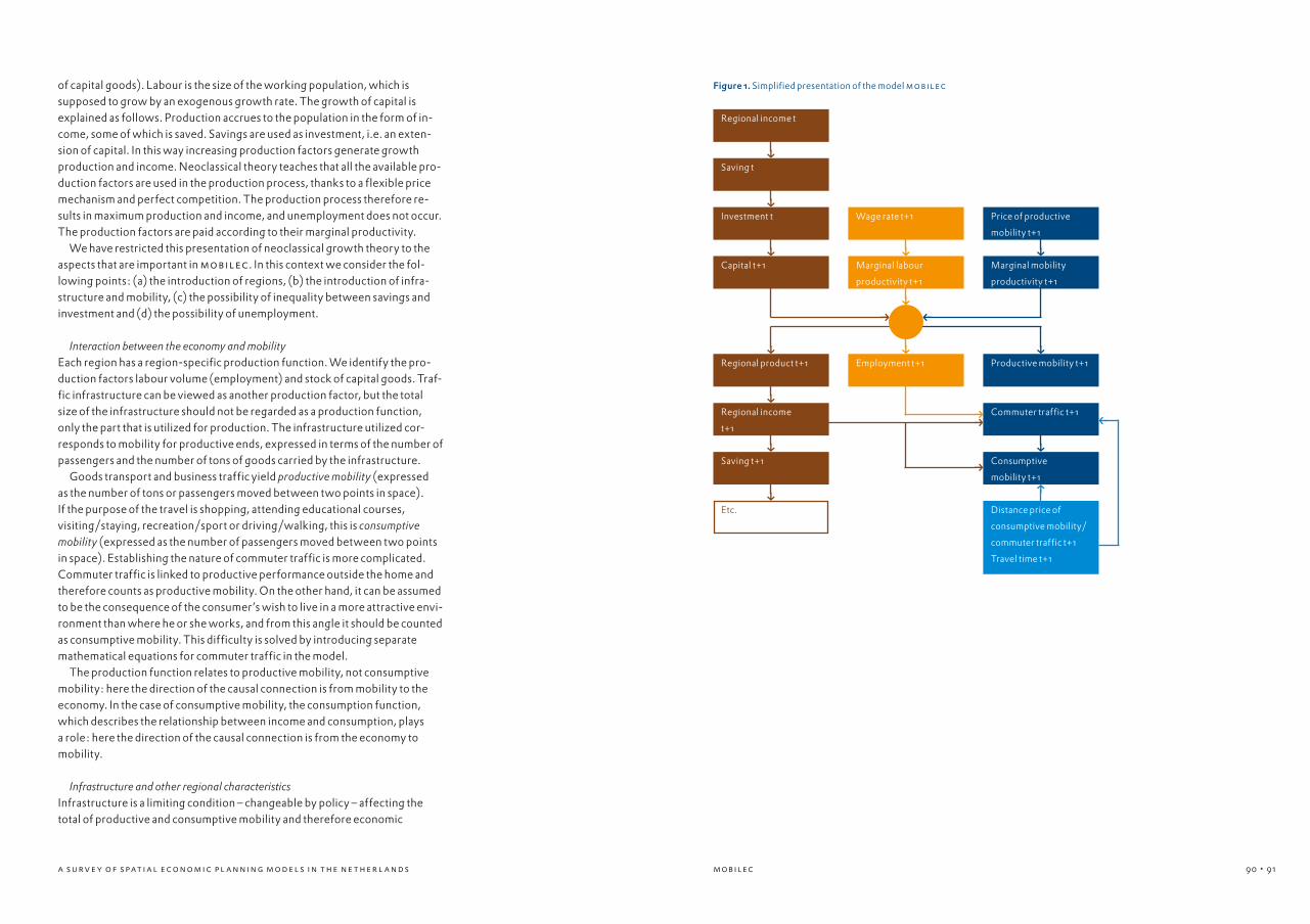
90 a s u rv e y o f s pat i a l eco n om i c p l a nni n g mo d el s i n t he ne t her l a nd s • 9190
of capital goods). Labour is the size of the working population, which is supposed to grow by an exogenous growth rate. The growth of capital is explained as follows. Production accrues to the population in the form of in-come, some of which is saved. Savings are used as investment, i.e. an exten-sion of capital. In this way increasing production factors generate growth production and income. Neoclassical theory teaches that all the available pro-duction factors are used in the production process, thanks to a flexible price mechanism and perfect competition. The production process therefore re-sults in maximum production and income, and unemployment does not occur. The production factors are paid according to their marginal productivity. We have restricted this presentation of neoclassical growth theory to the aspects that are important in mobilec. In this context we consider the fol-lowing points: (a) the introduction of regions, (b) the introduction of infra-structure and mobility, (c) the possibility of inequality between savings and investment and (d) the possibility of unemployment.
Interaction between the economy and mobilityEach region has a region-specific production function. We identify the pro-duction factors labour volume (employment) and stock of capital goods. Traf-fic infrastructure can be viewed as another production factor, but the total size of the infrastructure should not be regarded as a production function, only the part that is utilized for production. The infrastructure utilized cor-responds to mobility for productive ends, expressed in terms of the number of passengers and the number of tons of goods carried by the infrastructure. Goods transport and business traffic yield productive mobility (expressed as the number of tons or passengers moved between two points in space). If the purpose of the travel is shopping, attending educational courses, visiting/staying, recreation/sport or driving/walking, this is consumptive mobility (expressed as the number of passengers moved between two points in space). Establishing the nature of commuter traffic is more complicated. Commuter traffic is linked to productive performance outside the home and therefore counts as productive mobility. On the other hand, it can be assumed to be the consequence of the consumer’s wish to live in a more attractive envi-ronment than where he or she works, and from this angle it should be counted as consumptive mobility. This difficulty is solved by introducing separate mathematical equations for commuter traffic in the model. The production function relates to productive mobility, not consumptive mobility: here the direction of the causal connection is from mobility to the economy. In the case of consumptive mobility, the consumption function, which describes the relationship between income and consumption, plays a role: here the direction of the causal connection is from the economy to mobility.
Infrastructure and other regional characteristicsInfrastructure is a limiting condition – changeable by policy – affecting the total of productive and consumptive mobility and therefore economic
Figure 1. Simplified presentation of the model mobilec
mobilec
Regional income t
gSaving t
gInvestment t
gCapital t+1
gRegional product t+1
g
gSaving t+1
gEtc.
Wage rate t+1
gMarginal labour
productivity t+1
gEmployment t+1
Price of productive
mobility t+1
gMarginal mobility
productivity t+1
gProductive mobility t+1
Commuter traffic t+1
gConsumptive
mobility t+1
Distance price of
consumptive mobility/
commuter traffic t+1
Travel time t+1
i
hff
f
gf h
Regional income
t+1

92 a s u rv e y o f s pat i a l eco n om i c p l a nni n g mo d el s i n t he ne t her l a nd s • 9392
development. Before maximum mobility is reached, the limiting effect of infrastructure is revealed in the form of increased travel time and mobility cost. Mobility cost is defined as the generalized transport cost per passenger or per ton (in the case of freight transport). It consists of two parts, travel- distance cost (or the distance cost of mobility) and travel-time cost; travel- time cost is the result of evaluating travel time in monetary terms (Ministry of Transport, Public Works and Water Management 1996). The smaller the difference between actual mobility and maximum possible mobility (infra-structure capacity), the lower the speed of transport and the greater the travel-time cost. The type of infrastructure imposes restrictions on the means of transport and its speed, which are also expressed in the mobility cost. The model makes use of origin-destination matrices where the quality of accessibility within and between regions is expressed in terms of travel distance, travel time, travel-distance cost and travel-time cost, based on an infrastructure network. It cannot assign transport flows to specific stretches of infrastructure. It generates the flows of transport within a region and between pairs of regions. It takes into account the fact that a region’s infra-structure is utilized by transit traffic between other regions. Infrastructure is one of the factors that characterize regions. Other regional characteristics in the model are technological development, production struc-ture, urbanization (agglomeration economies and diseconomies), level of wage rates, existence of recreation areas, metropolitan character, per capita employment (in connection with commuting), investment premiums and geographical position. Their influence on the economy and mobility is also taken into consideration.
Specification of the modelThe specification of the model is as follows (for a mathematical presentation of the model see Van de Vooren 2004). Regional income in period t determines regional (private) savings in period t, which – depending on the balance of government spending and taxes levied in the region and the region’s balance of payments - are used as (private) investment. To what extent savings are used as investment in the region or elsewhere depends on the capital rate of return in relation to that in other regions. Regional (private) investment is just an extension of the (private) stock of capital goods; hence in the case of positive investments the region has a larger stock of capital goods at its disposal at the beginning of the next period t+1 than at the beginning of period t. Neoclassical theory teaches that marginal labour productivity determines the (flexible) wage rate. This relationship is reversed in mobilec in order to simulate the possibility of unemployment. The wage rate, agreed by employ-ers and employees, is considered as an exogenous (non-flexible) variable and determines marginal labour productivity. The price of productive mobility determines marginal mobility productivity. The stock of capital goods, marginal labour productivity and marginal mobility productivity in period t+1 – given the production function –
simultaneously determine regional product, employment and productive mobility in period t+1. The state of technology, the regional structure of pro-duction and the degree of urbanization in period t+1 are exogenous. Regional product accrues to the population in the form of regional income, which influ-ences consumptive mobility and commuter traffic. Consumptive mobility also depends on the distance cost of consumptive mobility and travel time as well as the region’s metropolitan character and recreation facilities in relation to other regions. Commuter traffic also depends on the distance cost of com-muter traffic and travel time, as well as per capita employment in the region in relation to other regions. At this point we have reached the end of the cycle of period t and the pro-cess starts all over again: regional income determines regional savings in period t+1, which can be used as investment in the region or elsewhere, and so on. Thus the model simulates a continuous process of development in the economy and mobility. Travel time and mobility costs rise as a result of increasing utilization of the available infrastructure, which has a negative influence on the growth of the economy and mobility. Substitution can take place between transport modes. Use of a certain mode depends not only on its mobility cost but also on the mobility costs of other modes (consumptive mobility and commuter traffic: distance costs of mobility and travel time instead of mobility costs). The demand for transport is considered mainly as a derived demand from the level of economic activity. The model computes the demand for labour and productive mobility based on the production function and the equations for marginal labour productivity and marginal mobility productivity. The results are as follows:
· the demand for labour depends on regional product and the wage rate;· the demand for productive mobility of goods (transport of goods)
depends on the regional product and the cost of productive mobility of goods;
· the demand for productive mobility of passengers (business traffic) depends on regional product and the cost of productive mobility of passengers.
The model, then, generates the demand for productive mobility as a derived demand, but regional product is endogenous. Consumption mobility and commuter traffic are considered as a derived demand from regional income, which is also an endogenous variable.
Endogenous and exogenous variablesThe main output that the model produces consists of the following variables:
· regional product/income, employment and investment;· transport of goods by lorry, train and ship (productive mobility) within
regions and between regions;· transport of passengers by car, train and bus/tram/metro within a region
and between regions, split up into business traffic (productive mobility), commuter traffic and other traffic (consumptive mobility).
mobilec

94 a s u rv e y o f s pat i a l eco n om i c p l a nni n g mo d el s i n t he ne t her l a nd s • 9594
These regional variables can be aggregated into national variables. They are, by definition, endogenous.
Other endogenous variables are:· travel time by lorry and bus/tram;· mobility costs of productive mobility, distance costs of consumptive
mobility and commuter traffic;· marginal labour productivity and marginal mobility productivity;· stock of (private) capital goods and rate of return on capital.
The costs of productive mobility (per passenger or per ton) between and within regions consist of travel-distance cost and travel-time cost. The prices of consumptive mobility and commuter traffic only include travel-distance cost. Travel-distance cost per kilometre, distances within a region and be-tween regions, and average load per lorry, train and ship/average number of passengers by car are exogenous, as are public transport tariffs. Travel-time cost depends on travel time, which is endogenous in the case of road traffic and exogenous in the case of other traffic. The travel time of road traffic is determined by the extent to which road capacity is utilized. Travel time (in-cluding waiting times) by train is considered as an exogenous variable, as it is not directly determined by the utilization of railway infrastructure. Travel time by ship (including waiting times at locks) is considered as an exogenous variable, as waterway infrastructure generally has overcapacity. All the regional characteristics are represented by exogenous variables, except per capita employment, since employment is an endogenous variable.
Estimation and implementationmobilec-Netherlands (there is also a mobilec-Belgium and a mobilec-Benelux) identifies 43 regions: 40 ‘corop’ regions in the Netherlands, the neighbouring countries of Belgium/Luxemburg, Germany, and France. The model does not distinguish between industries but it does include a variable indicating the regional production structure, which influences the economy and transport. This variable is taken exogenously. Different changes in the regional production structure can be taken into account in a scenario analysis. Transport policy does not generally produce fundamental changes in production structure, so it is not unacceptable for this variable to be regarded as exogenous in this respect. Statistical data are needed for the base period of the model, 1991–1993. The main statistical sources are Netherlands Statistics’ Regional Annual Economic Data for the economic variables, its National Travel Survey for the passenger transport variables, and data from the Dutch consultancy nea for the goods transport variables (Netherlands Statistics does not have regional data on transport of goods). We obtained the values of the coefficients and intercepts for the model in the base period 1991-1993 as follows:
1. Some coefficients (production elasticities in the production function) were quantified on the basis of economic theory.
2. Some coefficients (including income, distance cost and travel-time elasticities) were assigned values from empirical studies by other authors.
3. One coefficient (changes in travel time related to changes in the utilization of road capacity) has an a priori value. We found from a sensitivity analysis that multiplication of the a priori value by 0.5 and 1.5 has hardly any effect on the growth rates of mobility and the economy. (Meanwhile we have refined the relevant equation, enabling the a priori value to be replaced with an estimation using regression analysis).
4. The remaining coefficients were estimated using regression analysis. All values of the coefficients have the right sign and are significant at a level of 5%, with one exception.
5. The values of the intercepts (the constant part on the right-hand side of an equation) are such that each equation in the model yields the actual value of the dependent variable in the base period.
CasesWe present three cases: (a) a scenario analysis, (b) a computation of the effects of transport policy and (c) a computation of the effects of an infra-structure project including a cost-benefit analysis.
Scenario analysisAs an illustration we present two possible scenarios, assigning appropriate values to the exogenous variables. The first illustration is a scenario for a socio-economic environment with the following main characteristics:
1. Technological development is 2.25% over a three-year period. The state of technology is a quantity defined in mobilec.
2. The share of labour-intensive sectors (especially the service sector) in regional product increases over a three-year period by 0.75 of the increase in this share over the preceding three-year period.
3. The real wage rate rises by 1% a year.
Given the first two characteristics we refer to this scenario as a Moderately Innovative Service Economy. Using the model we can calculate that this socio-economic environment scenario, policy remaining unchanged, yields an average economic growth of 2.07% per year in the Netherlands over the 1995–2030 period. The interaction between the economy and mobility is taken into account. Table 1 (column 2) shows the results for the economy and mobility in the North Limburg region (the cd-rom gives a brief description and explanation of Tables 1, 2 and 3).
The second illustration is a scenario for a socio-economic environment derived from the European Coordination scenario of the Netherlands Bureau
mobilec

96 a s u rv e y o f s pat i a l eco n om i c p l a nni n g mo d el s i n t he ne t her l a nd s • 9796
for Economic Policy Analysis (cpb 1997). This scenario assumes, among other things, average economic growth in the Netherlands of 2.75% a year over the 1995-2020 period. If we take this 2.75% economic growth as our starting point, policies to stimulate the economy of a region will have no generative effects, only distributive ones: as regional policy can raise the region’s regio-nal product but the national product is quantitatively fixed in advance in the cpb scenario, this goes at the expense of other regions’ regional product – in other words it has only distributive effects. In order to enable generative effects to be included in the cpb scenario we proceed as follows. The cpb assumes an average rise in the real wage rate of 1.7% annually in its European Coordination scenario. We adopt this assumption and retain the second characteristic of the first scenario, the Moderately Innovative Service Economy. Given these assumptions, mobilec finds that, policy remaining unchanged, technological development needs to be 4.15% per three-year period in order to achieve an average economic growth of about 2.75% a year in the Netherlands. Hence 2.75% economic growth is no longer a starting point but a result of assumptions on technological development, as well as increases in the share of labour-intensive sectors and wage rises. The main characteristics of the cpb scenario are set as follows:
1. Technological development is 4.15% over a three-year period.2. The share of labour-intensive sectors (especially the service sector)
in regional product increases over a three-year period by 0.75 of the increase in the share over the preceding three-year period.
3. The real wage rate rises by 1.7% a year.
Now that the underlying characteristics are set instead of economic growth, generative effects of regional policy can be calculated for the cpb scenario. Table 1 (column 3) shows the results of the cpb scenario for the economy and mobility in the North Limburg region.
Effects of transport policyIn view of the debate on possible national transport policies we formulate the following policy variants for the 2000–2030 period as an illustration:
1. a reference variant: constant road capacity, constant real travel-distance cost per kilometre and constant travel time by train and ship;
2. an increase in road capacity such that travel time for road traffic does not rise in spite of increasing traffic; also constant real travel-distance cost per kilometre and constant travel time by train and ship;
3. a rise in mobility tariffs: real travel-distance cost per kilometre by car and lorry rises by 3% a year and for other modes of transport by 1% per year; also constant road capacity and constant travel time by train and ship;
4. promotion of public transport: an increase in frequency and speed (modern vehicles, priority measures, dedicated lanes etc.) such that travel time by train and bus/tram/metro (including waiting time) falls by 1% a year; also constant road capacity, constant real travel-distance cost per kilometre and constant travel time by ship.
mobilec
1. Transport growth has been cal-
culated on the basis of passenger
numbers or quantities in tons.
The transport flows by car, lorry
and bus include transit traffic
through the region except transit
traffic from a foreign country
to another foreign country. The
transport flows by train and ship
exclude transit traffic. Passenger
transport excludes foreign coun-
tries.
2. See note 1 to Table 1.
3. Including tram and metro
Table 1. Average growth per annum (in %) of real regional product, employment and trans-
port of goods and passengers by mode of transport in North Limburg over the 1995–2030
period, based on two socio-economic scenarios and unchanged policy1
Moderately Innovative
Service Economy
European Coordination
(cpb)
Regional product 1.91 2.65
Employment 0.90 0.93
Goods transport
by lorry 1.60 2.12
by train 1.65 2.37
by ship 2.62 3.06
Passenger transport
by car 0.86 1.09
by train 0.04 0.08
by bus -0.10 -0.26
Table 2. Average growth per annum (in %) of regional product, employment and transport
of goods and passengers by mode of transport in Greater Amsterdam over the 2000–2030
period, based on the Moderately Innovative Service Economy2
Reference
variant
Increase in road
capacity
Rise in mobility
tariffs
Promotion of public
transport
Regional product 2.12 2.16 1.98 2.14
Employment 1.11 1.15 0.97 1.13
Goods transport
by lorry 1.36 1.55 0.50 1.37
by train 2.02 2.05 0.98 2.11
by ship 2.29 2.31 1.70 2.30
Passenger transport
by car 0.87 1.10 -0.08 0.83
by train 0.13 0.09 -0.38 1.90
by bus 3 -0.19 0.04 -0.01 1.39

98 a s u rv e y o f s pat i a l eco n om i c p l a nni n g mo d el s i n t he ne t her l a nd s • 9998
By way of example Table 2 shows the quantitative effects of these four policy variants for the Greater Amsterdam region based on the Moderately Innovative Service Economy scenario. The differences between the policy variants seem small, but they are considerable in absolute terms. Mean annual growth in employment, for example, increases from 1.11% in the reference variant to 1.15% in the road variant, resulting in about 9,300 more jobs in 2030, i.e. 1.8% of the employment in Greater Amsterdam in 2000. It is possible to calculate the effects of combinations of these policy variants and those of more complex policy variants.
Effects of infrastructure projectsmobilec specifies transport flows within and between regions without rela-ting them to individual stretches of infrastructure. Computational rules have therefore been formulated to express the consequences of an infrastructure project to increase infrastructure capacity in a region. The model then calcu-lates the reductions in travel time for the transport flows in question due to the increase in regional infrastructure capacity. A more precise estimation of the effect of increasing of the capacity of a specific stretch on travel time can be made using a traffic model as a starting point. This is particularly important in the case of small improvements to infrastructure. The traffic model estimates the initial reduction in travel time as a result of increasing the capacity of a specific stretch of infrastructure. Computational rules express this in terms of reductions of travel time within and between regions, which are fed into mobilec. Based on these, mobilec calculates the effects on the economy and mobility over time, taking into account further changes in travel time (for coupling of transport models see Van de Vooren 2003).
This method of linking a traffic model to mobilec has been applied to many stretches of motorway in the Netherlands (using the New Regional Model of the Dutch Ministry of Transport, Public Works and Water Management 1997, as the traffic model). We illustrate it with a computation of the effects on regional product of three increases in capacity on the Barneveld-Deventer and Deventer-Hengelo stretches of the A1 motorway. The computations are based on the European Coordination scenario and the reference variant of policy. The following alternatives were examined:
· Alternative 0: Barneveld-Deventer 2x2 stretches and Deventer-Hengelo 2x2 stretches;
· Alternative 1: Barneveld-Deventer 2x3 stretches and Deventer-Hengelo 2x2 stretches;
· Alternative 2: Barneveld-Deventer 2x3 stretches and Deventer-Hengelo 2x3 stretches;
· Alternative 3: Barneveld-Deventer 2x4 stretches and Deventer-Hengelo 2x3 stretches;
As regards the regional product of Southwest Overijssel over the 2018-2020 period, for example, Table 3 shows that this is 3.9 million euros higher each
mobilec
gEconomic effect of
project
Travel time with
project
gRegional product/
Employment with
project
f h
Production of travel
time by project
Traffic model
g
Regional product/
Employment without
project
Travel time without
project
g
mobilec
gf h
f
Figure 2. Linking a traffic model to the model mobilec
Table 3. Average increase in real regional product per year (in million euros, 2002 price
levels) over the 2018–2020 and 2027–2029 periods as a result of adopting an enlargement
alternative in 2018, based on the European Coordination scenario and the reference variant
of policy4
2018–2020 2027–2029
Alt. 1 Alt. 2 Alt.3 Alt. 1 Alt. 2 Alt. 3
Southwest Overijssel 3.9 4.0 4.7 4.4 4.2 5.0
Twente 14.5 19.0 21.5 17.3 22.2 25.1
Veluwe 9.0 9.5 10.2 4.6 4.6 4.2
Utrecht 7.1 7.9 8.4 4.7 5.3 5.2
Greater Amsterdam 3.9 4.6 4.9 3.4 4.2 4.4
Greater Rotterdam 3.6 4.7 5.3 3.4 4.6 5.1
Rest of the Netherlands 12.3 14.4 16.3 4.3 5.6 5.8
total netherlands 54.3 64.1 71.4 42.1 50.6 54.7
Table 4. Cost-benefit analysis of enlargement alternatives for the A1 motorway,
Barneveld-Deventer and Deventer-Hengelo stretches
Alternative 1: Alternative 2: Alternative 3:
compared with Alt. 0 compared with Alt. 1 compared with Alt. 2
Benefit – cost of
maintenance (b) 640 128 36
Construction cost (c) 208 36 85
b / c 3.1 3.6 0.4
4. The totals for the regions may
not add up to the figures for
Total Netherlands as a result of
rounding.

100 a s u rv e y o f s pat i a l eco n om i c p l a nni n g mo d el s i n t he ne t her l a nd s • 101100
year (on average) in Alternative 1 than in the null alternative. The increase over the whole period is 3 x 3.9 = 11.7 million euros. If we calculate the effects in terms of percentages of regional product we get very small numbers, e.g. 0.1% for Southwest Overijssel and Twente, and even less for other regions. The absolute differences between the annual effects of the alternatives are small, but totalled over a period of 50 years they are substantial, especially when compared with the once-only construction cost of the enlargement. This is the starting point for a cost-benefit analysis. We calculate the benefit as the total of the increase in the Dutch domestic product and welfare creation due to the reduction in travel time for consump-tive mobility and commuter traffic not expressed in the domestic product. The cost of maintenance has to be deducted from the benefit. The net benefit is then compared with the construction cost. We use a real discount rate of 4% as prescribed in the Netherlands.
We conclude from Table 4 that the increase in road capacity under Alternative 1 is socially profitable, but the larger increase under Alternative 2 is prefera-ble. The further increase under Alternative 3 is not socially profitable.
Conclusions and final remarksThe model is founded on neoclassical growth theory. In this context we con-sider the following points: (a) the introduction of regions, (b) the introduc-tion of infrastructure and mobility, (c) the possibility of inequality between savings and investment and (d) the possibility of unemployment. The result is a dynamic, interregional model that specifies the relationships between the economy, mobility, infrastructure and other regional characteristics. mobilec offers a new approach to the interaction between transport and the economy. It enables the effects of transport policy on transport to be estimated better, as it also takes indirect effects into account, i.e. those via the economy. Another feature of the model is its dynamic nature. Calculating transport and economic variables in successive periods is important to transport policy and spatial planning. Such calculations are a necessary precondition for apply-ing cost-benefit analysis to infrastructure projects. The model calculates the development of transport and the economy, driven by investment and technological development, as a continuous pro-cess in which the regions affect one another. Travel time and mobility costs rise as a result of increasing utilization of the available infrastructure, which has a negative influence on the growth of the economy and mobility. The process of development is also influenced by travel-distance costs and other regional characteristics besides infrastructure. Using the model a scenario analysis can be carried out, generating time paths for transport and economic variables for the 40 regions of the Netherlands. The effects of transport policy, including infrastructure pro-jects, on transport and the economy in successive periods can be calculated. The results of this, and the effects of changes in other regional characteristics,
can be used in spatial planning. We have carried out several scenario analyses and effect calculations since 1999. The quantitative results were always plau-sible in the opinion of experts and users.
A model is never finished. We are currently incorporating the various options for financing infrastructure improvements and spending the revenue from a levy on mobility. We have calculated the effects of these on transport and the economy using mobilec-Belgium. We are experimenting with calculations for sub-regions within corop regions. We intend to examine the possibility of applying less restrictive production functions than the present Cobb-Douglas type. These production functions offer the advantage of calculating the equations for the time paths of the economic and transport variables. We are preparing a more recent base period for the model along with new esti-mates for the coefficients. Other roads for improvement that are considered are adding a labour market and the disaggregation of the total economy into a number of industries. Finally, we want to check the overall fit of the model, i.e. to examine how the time paths for the transport and economic variables fit actual developments in the past.
mobilec
References
cpb (1997), Economie en fysieke omgeving;
beleidsopgaven en oplossingsrichtingen
1995–2020, Den Haag: Centraal Planbureau.
Ministry of Transport, Public Works
and Water Management (1996), Handboek
Economische Effecten Infrastructuur,
Rotterdam: V&W-Platform Economie/
Adviesdienst Verkeer en Vervoer
Ministry of Transport, Public Works
and Water Management (1997), Handboek
Nieuw Regionaal Model, Rotterdam:
Adviesdienst Verkeer en Vervoer.
Van de Vooren, F.W.C.J. (2003), Koppeling
van transportmodellen, Research paper
2003-002, University of Antwerp,
Department of Transport and Regional
Economics.
Van de Vooren, F.W.C.J. (2004),
‘Modelling transport in interaction with the
economy’, Transportation Research Part E
40/5: 417-37.

102
regina
A model of economic
growth prospects for
Dutch regions

104
regina. a model of economic growth prospects for dutch regions Olaf Koops, Jos Muskens
IntroductionWhy do some regions perform better in terms of economic growth than others? This question has been asked by economists ever since Adam Smith wrote his Wealth of Nations, and many answers have been given. Most em-pirical research involves analysing differences in economic growth between countries, but the explanations for these differences at national levels may differ markedly from those at the more detailed, regional level. New spatial economic theories evolved in the 1990s, thanks to the work of Paul Krugman and others in the New Economic Geography (neg) litera-ture. Attempts to apply this theory to empirical research are still scarce in the Netherlands and elsewhere, but progress has been made recently. Examples of neg-based models which analyse regional economic growth in the Nether-lands (in particular r aem and remi) can be found elsewhere in this book. The level of geographical detail in these models is still rather high. There are not many models available for the municipal level (the Netherlands has just under 500 municipalities). Local authorities are increasingly expressing an interest in the economic prospects for their town or region, mainly because of the growing responsibilities upon them resulting from institutional decen-tralization in the Netherlands. To decide upon regional policies the author-ities need to know what the differences are in economic growth between regions and how they can be explained. Central government needs to know whether generic policy measures will help all the regions equally or whether some regions require specific measures. Private firms can use findings from empirical research to explore market areas or to help them decide where to locate or where to invest in real estate, housing or land. tno has been developing a regional model to analyse growth differences between regions in the Netherlands since the early 1990s.1 The aim is (1) to describe growth differences between regions, (2) to explain these dif-ferences and (3) to forecast regional economic growth. The model has been updated recently and is now called regina. The main change in the structure of the model is the breakdown of regional levels in two steps. Step 1 divides the Netherlands into 40 ‘corop’ regions2 and analyses the differences in economic growth between these regions and the nation as a whole. Step 2 zooms in on the municipalities, comparing their economic growth to that in the immediate environment (the corop region, or the region within a certain travel time radius). This two-step system enables different explanations to be found for different regional levels. The next section describes the model in more detail. The third section takes one particular region in the Netherlands as an example of how regina works. Concluding remarks are given in the fourth section.
regina. A model of economic growth prospects for Dutch regions
1. See e.g. Louter et al. (1997).
2. The Netherlands consists of 40
corop regions, or nuts3 regions
under the eu classification.
• 105
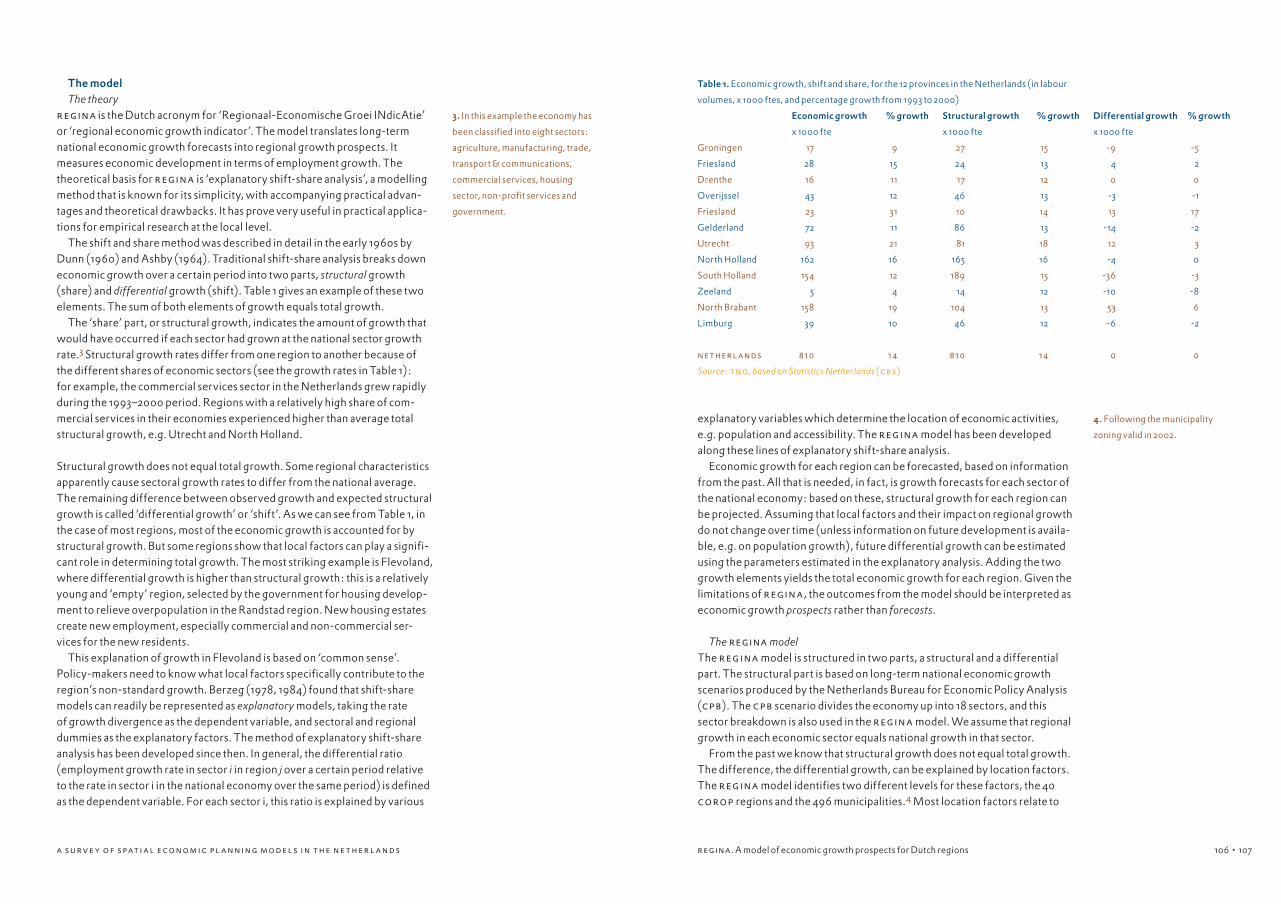
106 a s u rv e y o f s pat i a l eco n om i c p l a nni n g mo d el s i n t he ne t her l a nd s • 107106
The modelThe theory
regina is the Dutch acronym for ‘Regionaal-Economische Groei INdicAtie’ or ‘regional economic growth indicator’. The model translates long-term national economic growth forecasts into regional growth prospects. It measures economic development in terms of employment growth. The theoretical basis for regina is ‘explanatory shift-share analysis’, a modelling method that is known for its simplicity, with accompanying practical advan-tages and theoretical drawbacks. It has prove very useful in practical applica-tions for empirical research at the local level. The shift and share method was described in detail in the early 1960s by Dunn (1960) and Ashby (1964). Traditional shift-share analysis breaks down economic growth over a certain period into two parts, structural growth (share) and differential growth (shift). Table 1 gives an example of these two elements. The sum of both elements of growth equals total growth. The ‘share’ part, or structural growth, indicates the amount of growth that would have occurred if each sector had grown at the national sector growth rate.3 Structural growth rates differ from one region to another because of the different shares of economic sectors (see the growth rates in Table 1): for example, the commercial services sector in the Netherlands grew rapidly during the 1993–2000 period. Regions with a relatively high share of com-mercial services in their economies experienced higher than average total structural growth, e.g. Utrecht and North Holland.
Structural growth does not equal total growth. Some regional characteristics apparently cause sectoral growth rates to differ from the national average. The remaining difference between observed growth and expected structural growth is called ‘differential growth’ or ‘shift’. As we can see from Table 1, in the case of most regions, most of the economic growth is accounted for by structural growth. But some regions show that local factors can play a signifi-cant role in determining total growth. The most striking example is Flevoland, where differential growth is higher than structural growth: this is a relatively young and ‘empty’ region, selected by the government for housing develop-ment to relieve overpopulation in the Randstad region. New housing estates create new employment, especially commercial and non-commercial ser-vices for the new residents. This explanation of growth in Flevoland is based on ‘common sense’. Policy-makers need to know what local factors specifically contribute to the region’s non-standard growth. Berzeg (1978, 1984) found that shift-share models can readily be represented as explanatory models, taking the rate of growth divergence as the dependent variable, and sectoral and regional dummies as the explanatory factors. The method of explanatory shift-share analysis has been developed since then. In general, the differential ratio (employment growth rate in sector i in region j over a certain period relative to the rate in sector i in the national economy over the same period) is defined as the dependent variable. For each sector i, this ratio is explained by various
explanatory variables which determine the location of economic activities, e.g. population and accessibility. The regina model has been developed along these lines of explanatory shift-share analysis. Economic growth for each region can be forecasted, based on information from the past. All that is needed, in fact, is growth forecasts for each sector of the national economy: based on these, structural growth for each region can be projected. Assuming that local factors and their impact on regional growth do not change over time (unless information on future development is availa-ble, e.g. on population growth), future differential growth can be estimated using the parameters estimated in the explanatory analysis. Adding the two growth elements yields the total economic growth for each region. Given the limitations of regina, the outcomes from the model should be interpreted as economic growth prospects rather than forecasts.
The regina modelThe regina model is structured in two parts, a structural and a differential part. The structural part is based on long-term national economic growth scenarios produced by the Netherlands Bureau for Economic Policy Analysis (cpb). The cpb scenario divides the economy up into 18 sectors, and this sector breakdown is also used in the regina model. We assume that regional growth in each economic sector equals national growth in that sector. From the past we know that structural growth does not equal total growth. The difference, the differential growth, can be explained by location factors. The regina model identifies two different levels for these factors, the 40 corop regions and the 496 municipalities.4 Most location factors relate to
3. In this example the economy has
been classified into eight sectors:
agriculture, manufacturing, trade,
transport & communications,
commercial services, housing
sector, non-profit services and
government.
4. Following the municipality
zoning valid in 2002.
regina. A model of economic growth prospects for Dutch regions
Table 1. Economic growth, shift and share, for the 12 provinces in the Netherlands (in labour
volumes, x 1000 ftes, and percentage growth from 1993 to 2000)
Economic growth
x 1000 fte
% growth Structural growth
x 1000 fte
% growth Differential growth
x 1000 fte
% growth
Groningen 17 9 27 15 -9 -5
Friesland 28 15 24 13 4 2
Drenthe 16 11 17 12 0 0
Overijssel 43 12 46 13 -3 -1
Friesland 23 31 10 14 13 17
Gelderland 72 11 86 13 -14 -2
Utrecht 93 21 81 18 12 3
North Holland 162 16 165 16 -4 0
South Holland 154 12 189 15 -36 -3
Zeeland 5 4 14 12 -10 -8
North Brabant 158 19 104 13 53 6
Limburg 39 10 46 12 -6 -2
netherl ands 810 14 810 14 0 0
Source: tno, based on Statistics Netherlands (cbs)
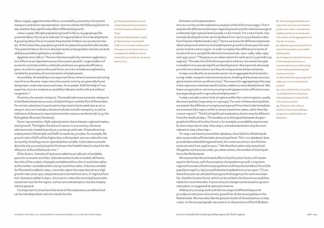
108 a s u rv e y o f s pat i a l eco n om i c p l a nni n g mo d el s i n t he ne t her l a nd s • 109108
labour supply, agglomeration effects, accessibility, proximity of economic mainports and sector representation. regina checks the following factors to see whether they significantly affect differential growth: Labour supply. We take population growth in the 15–64 age group (the potential labour force) as an indicator of regional labour force developments. A growing labour force increases the potential of labour as a production fac-tor. At the same time, population growth increases the potential sales market. The potential labour force (in absolute terms) and population density are both added as possible explanatory variables.5
Agglomeration effects. The neg literature explicitly mentions agglomera-tion effects as an important source of economic growth. Large numbers of economic activities within a relatively small area can generate efficiency gains. In order to capture this push factor, regina includes an explanatory variable for proximity of concentrations of employment. Accessibility. Accessibility is an important factor when it comes to attracting new firms to the area: major sites of economic activity are generally found along major roads near towns and cities, for example. With the help of tno expertise, regina analyses accessibility indicators both with and without congestion.6 Proximity of economic mainports. The model takes two economic mainports in the Netherlands into account, Schiphol Airport and the Port of Rotterdam. For certain industries it is particularly important to be located near an air or sea port. regina includes a distance indicator to both mainports, as well as indicators of distance to important economic areas across the border (e.g. the Ruhrgebiet, Brussels/Antwerp). Sector representation. High regional sector shares hamper regional employ-ment growth. The higher the share of a sector in an economy, the more jobs have to be created to produce a certain growth rate: if manufacturing employment in Rotterdam and Delft increases by 500 jobs, for example, the growth rate in Delft will be higher than in Rotterdam. regina takes this into account by including a sector specialization variable. It also takes economic diversity into account (using the Hirshman-Herfindahl Index) to check for the influence of diversified sector mix.7 Other factors. Intensity of land use is added as an indicator of available space for economic activities. Suburbanization is also included, defined as the ratio of the number of people reachable within a short travel time radius to the number reachable within a long travel time radius. A dummy variable for Flevoland is added in step 1, since this region has experienced very high growth rates since 1970, simply because it started from zero. A ‘regional func-tion’ dummy is added in step 2: this is set to 1 when the municipality provides several services for the region, such as care and education, but also employ-ment in general. It is important to stress here that some of the explanatory variables listed can be interdependent. regina checks for this.
Estimation and implementationregina carries out the explanatory analysis of the shift in two stages. First it explains the differences between regional growth and the national average at a relatively high regional level (usually corop level). For corop level, tno recently developed a time-series database from 1970 to 2000 based on data from Statistics Netherlands (cbs),8 hence we know the difference between observed growth and structural employment growth in those years for each sector in each corop region. In order to explain this difference in terms of location factors, we split the data into three periods, 1970–1983, 1983–1993 and 1993–2000.9 This gives us 120 observations for each sector (3 periods x 40 regions). The selection of the three periods is arbitrary, but some time span is needed to incorporate significant developments. More periods obviously provide more observations, but they do not guarantee better estimates. In step 1 we identify six economic sectors at an aggregate level (manufac-turing, trade, transport and communications, banking and business services, government and non-profit services). The reason for aggregating in this way is that regression estimates tend to be less stable at a more detailed level. We leave out agriculture, since structural growth appears to be sufficient to ana-lyse regional growth in agricultural employment.10
In step 2 we take a closer look at regions within the corop regions, usually the municipalities (separately or in groups). For each of these municipalities we explain the difference in employment growth from that in the immediate environment (the region within a certain travel time radius, rather than the corop region).11 The list of significant explanatory factors may be different from the results of step 1. This enables us to distinguish between the geo-graphical effects of location factors: for example, accessibility aspects may be more important in step 1 than step 2, and suburbanization may be more relevant in step 2 than step 1. For step 2 we have to use another database, since Statistics Netherlands does not provide sufficient data at municipal level. This ‘lisa database’ does provide data at detailed regional level, for numerous sectors, but the time series are only from 1996 to 2002.12 We therefore select only one period. Altogether we have just under 500 observations, the number of municipali-ties in the Netherlands. We assume that the estimated effect of each location factor will remain equal in the future, with the exception of population growth. Long-term regional forecasts of both total population and the potential labour force (the population aged 15–64) are published and updated every two years.13 From these forecasts we calculate future growth divergences for each municipa-lity. Another location factor which can be varied in the future is accessibility, related to travel time data. Future network changes can be based on govern-ment plans, or suggested as optional scenarios. Adding structural growth with the two steps of differential growth provides an indication of economic growth for all the municipalities in the Netherlands. We now describe the general results of the estimations in step 1 and 2. In the next paragraph we zoom in on the province of North Brabant
5. The potential labour force is
used instead of the actual labour
force for reasons of data availa-
bility.
6. See also Manshanden (1996).
7. The Hirshman-Herfindahl
Index (hhi) consists of the sum of
the square sector shares; the hhi
is analysed for different lists of
sectors (8-sector shares, 18-sector
shares, etc.).
8. The tno Regio Database con-
tains time-series on investments,
production, labour volumes and
added value for 37 economic sec-
tors, which can be aggregated into
the 18 cpb sectors.
9. 1983 and 1993 are years of reces-
sion in the economic cycle of the
Netherlands.
10. Compared to the list of sectors
in the example of section 2.1,
commercial services and housing
sector make up the banking and
business services.
11. We check that regional growth
adds up to corop and national
growth.
12. lisa is the Dutch acronym for
‘Landelijk Informatie Systeem
Arbeidsplaatsen’ (national jobs
information system).
13. These are referred to in
Dutch as ‘primos bevolkings-
prognoses’, published by abf
Research.
regina. A model of economic growth prospects for Dutch regions

110 a s u rv e y o f s pat i a l eco n om i c p l a nni n g mo d el s i n t he ne t her l a nd s • 111110
to show what the results imply for employment growth in the municipalities there up to 2010, and how growth is distributed among structural growth and the two steps of differential growth. 14
Table 2 shows the estimation results from step 1 of the differential growth analysis in regina. It shows what factors explain the difference in employment growth between the corop regions and the Netherlands as a whole. As expected, growth in the potential labour force positively affects employment growth. A growing labour force induces labour potential as a production factor and at the same time increases the potential sales market. Not surprisingly, this latter appears to be particularly relevant to the trade sector. Sector specialization hampers employment growth significantly in all sectors, whereas economic diversity has no marked effect. Accessibility has been shown to be important, both nationally and internationally. Generally this means that growth in the peripheral regions of the country is hampered by their relative distance from the central regions but boosted by the relative proximity of economic centres across the border. Interestingly, proximity to Schiphol Airport or the Port of Rotterdam does not have a significant influ-ence. Manufacturing activities generally need more space, so it comes as no surprise that high intensity of land use negatively affects growth in manufac-turing employment. Table 3 shows the results of the estimation in step 2 of the differential growth analysis. Here regina explains the differences in employment growth between municipalities and their regions (within a 30-minute travel time radius).15 Again, growth in the potential labour force positively affects employment, but in the case of only three sectors this time; in the other three sectors total population growth appears to be significantly positive. This to some extent replaces the labour force variable, but in the government sector in particular it makes sense to take the number of people aged below 15 and above 64 into account. Sector specialization hampers employment growth again in all sectors except trade. Of special interest is the finding that, at this regional level, economic diversity has a negative effect on employment growth in the trade, transport and non-profit sectors and a positive effect on commercial services. This sector depends on relations with companies in all sectors, which explains the positive sign (although significant only at 15%). The other sectors have relations mainly with one or two other sectors. The prevalence of the agglomeration and clustering variable implies that commer-cial services benefit not only from economic diversity within the municipality but also from concentrations of employment in neighbouring municipalities. Suburbanization positively affects growth in trade and transport, a rather obvious finding. Land use intensity negatively affects growth in trade: this makes sense at the municipal level, since trade includes wholesale trade. Finally, three more variables appear to have an influence on the government sector: if a municipality provides several services for the region, it attracts relatively more government employment. The same holds true for the share of the commercial services sector. Density of commercial services corrects for that positive correlation.
regina. A model of economic growth prospects for Dutch regions
14. The parameter estimations as
shown in Tables 2 and 3 are linked
to the case for the purpose of
describing the model. They will
not necessary be the same for new
cases in the near future.
15. 30 minutes is close to the aver-
age commuting time, and corre-
sponds roughly with the size of the
corop areas.
16. Significant only at 15%
Table 2. Estimation results of regina, step 1, for each sector (standardized coefficients,
significant at 5%)
Explanatory variable Manufacturing Trade Transport &
comm.
Commercial
services
Government Non-profit
(constant) 1.05 0.65 1.30 0.49 0.72 0.81
Labour force growth 0.73 1.08 0.39 0.85 0.98 0.70
Labour force 0.27
Population density -0.20 0.31
Sector specialization -0.38 -0.54 -0.35 -0.60 -0.44 -0.26
National accessibility 0.40 0.20
Congestion 0.15
International
accessibility
0.22 0.16 0.17 -0.11
Intensity of land use -0.37
Dummy for Flevoland 0.20
R2 0.55 0.85 0.25 0.53 0.52 0.77
Source: tno
Table 3. Estimation results of regina, step 2, for each sector (standardized coefficients,
significant at 10%)
Explanatory variable Manufacturing Trade Transport &
comm.
Commercial
services
Government Non-profit
Constant 0.01 0.09 0.13 -0.27 -0.03 0.10
Labour force growth 0.33 0.28 0.23
Population growth 0.32 0.11 0.14
Population density -0.11
Sector specialization -0.11 -0.22 0.28 -0.40 -0.14
Economic diversity -0.10 -0.15 0.0916 -0.13
Agglomeration and
clustering
0.11
Suburbanization 0.16 0.13
Intensity of land use -0.23
Dummy regional
function
0.22
Specialization of com-
mercial services
0.15
Density of commercial
services
-0.14
R2 0.11 0.15 0.09 0.13 0.11 0.10
Source: tno
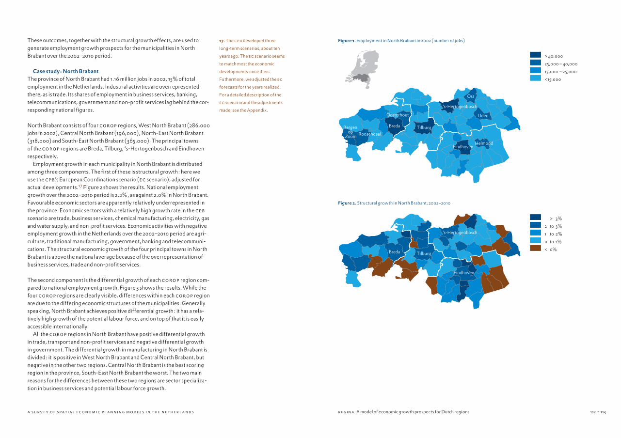
112 a s u rv e y o f s pat i a l eco n om i c p l a nni n g mo d el s i n t he ne t her l a nd s • 113112
These outcomes, together with the structural growth effects, are used to generate employment growth prospects for the municipalities in North Brabant over the 2002–2010 period.
Case study: North BrabantThe province of North Brabant had 1.16 million jobs in 2002, 15% of total employment in the Netherlands. Industrial activities are overrepresented there, as is trade. Its shares of employment in business services, banking, telecommunications, government and non-profit services lag behind the cor-responding national figures.
North Brabant consists of four corop regions, West North Brabant (286,000 jobs in 2002), Central North Brabant (196,000), North-East North Brabant (318,000) and South-East North Brabant (365,000). The principal towns of the corop regions are Breda, Tilburg, ‘s-Hertogenbosch and Eindhoven respectively. Employment growth in each municipality in North Brabant is distributed among three components. The first of these is structural growth: here we use the cpb’s European Coordination scenario (ec scenario), adjusted for actual developments.17 Figure 2 shows the results. National employment growth over the 2002–2010 period is 2.2%, as against 2.0% in North Brabant. Favourable economic sectors are apparently relatively underrepresented in the province. Economic sectors with a relatively high growth rate in the cpb scenario are trade, business services, chemical manufacturing, electricity, gas and water supply, and non-profit services. Economic activities with negative employment growth in the Netherlands over the 2002–2010 period are agri-culture, traditional manufacturing, government, banking and telecommuni-cations. The structural economic growth of the four principal towns in North Brabant is above the national average because of the overrepresentation of business services, trade and non-profit services.
The second component is the differential growth of each corop region com-pared to national employment growth. Figure 3 shows the results. While the four corop regions are clearly visible, differences within each corop region are due to the differing economic structures of the municipalities. Generally speaking, North Brabant achieves positive differential growth: it has a rela-tively high growth of the potential labour force, and on top of that it is easily accessible internationally. All the corop regions in North Brabant have positive differential growth in trade, transport and non-profit services and negative differential growth in government. The differential growth in manufacturing in North Brabant is divided: it is positive in West North Brabant and Central North Brabant, but negative in the other two regions. Central North Brabant is the best scoring region in the province, South-East North Brabant the worst. The two main reasons for the differences between these two regions are sector specializa-tion in business services and potential labour force growth.
17. The cpb developed three
long-term scenarios, about ten
years ago. The ec scenario seems
to match most the economic
developments since then.
Futhermore, we adjusted the ec
forecasts for the years realized.
For a detailed description of the
ec scenario and the adjustments
made, see the Appendix.
regina. A model of economic growth prospects for Dutch regions
Figure 1. Employment in North Brabant in 2002 (number of jobs)
Figure 2. Structural growth in North Brabant, 2002–2010
Breda Tilburg
Oss
Uden
Roosendaal
Eindhoven
Oosterhout
Helmond
‘s-Hertogenbosch
Bergen op
Zoom
> 3%
2 to 3%
1 to 2%
0 to 1%
< 0%
> 40,000
25,000 – 40,000
15,000 – 25,000
<15,000
Breda Tilburg
Eindhoven
‘s-Hertogenbosch

114 a s u rv e y o f s pat i a l eco n om i c p l a nni n g mo d el s i n t he ne t her l a nd s 114
The final component is the differential growth of each municipality compared to its regional environment. Figure 4 shows the results. In the Netherlands in general, growth rates in the cities lag behind those in the surrounding muni-cipalities. Relatively low population growth rates and relatively high sector specialization rates cause this phenomenon. Within North Brabant, Breda is an exception, with its relatively high growth in the potential labour force. Suburban municipalities generally have rapidly increasing labour forces and low specialization indices, and they benefit from the agglomeration advan-tages of a nearby large town: examples in North Brabant are Drimmelen, Dongen, Vught and Waalre. The differential growth rates in the various eco-nomic sectors are fairly similar, with the sole exception of government. This similarity is caused by the general influence of the increasing labour force. Eventually, all the growth components lead to overall employment growth for municipalities. Figure 5 shows the results of totalling all the components. The four principal towns will see above average growth because of their economic structure. The municipalities near the principal towns have the best prospects, relatively speaking, of employment growth, especially the regions north of Tilburg and Breda.
ConclusionsThe regina model helps to explain growth differences at low regional levels in the Netherlands. It translates national economic growth forecasts into regional growth prospects. regina has a detailed geographical level at which it can present outcomes and it takes the differing roles of location fac-tors at different geographical levels into account. This makes it a useful tool for assisting both national and regional authorities to make policy decisions and helping private firms to decide where to locate or what market areas to explore. The analytical structure of regina is quite straightforward, but its simplicity also brings along a number of drawbacks.
Firstly, regional growth prospects depend heavily on the national growth forecasts selected. The cpb scenarios make assumptions about international developments in politics, economics, demography, technology and socio-cultural factors, and as they were programmed about ten years ago they are far from up-to-date. New national long-term scenarios have not yet been published by cpb. Note that regina can regionalize growth figures at several regional levels.
Secondly, regina only takes account of external factors which determine differences in economic growth between regions; it cannot take factors directly linked to individual companies, e.g. migration, mergers or locations by major companies, into account. Individual company behaviour is hard to predict and only included in regina indirectly, through regional factors that determine the location of firms, e.g. congestion or available land. Furthermore, regina does not pick up all the interrelations on the regional labour market. It assumes that regional employment (labour demand) fol-
regina. A model of economic growth prospects for Dutch regions
Figure 3. Differential growth in the corop regions of North Brabant, 2002–2010
Figure 4. Differential growth in municipalities, 2002–2010
Breda Tilburg
Eindhoven
‘s-Hertogenbosch
> 1.50%
1.00 to 1.50%
0.75 to 1.00%
0.25 to 0.75%
0.00 to 0.25%
-0.40 to 0.00%
< -0.40%
Breda Tilburg
Eindhoven
‘s-Hertogenbosch
Figure 5. Total employment growth prospects for municipalities in North Brabant, 2002–2010
Breda Tilburg
Eindhoven
‘s-Hertogenbosch
> 1.00%
0,75 to 1.00%
0.50 to 0.75%
0.25 to 0.50%
0.00 to 0.25%
-0.50 to 0.00%
< -0.50%
> 3.75%
3.00 to 3.75%
2.25 to 3.00%
1.50 to 2.25%
0.75 to 1.50%
0.00 to 0.75
-0.75 to -0.00%
< -0.75%
• 115

116 a s u rv e y o f s pat i a l eco n om i c p l a nni n g mo d el s i n t he ne t her l a nd s
lows regional population (labour supply), while this causality can operate in the other direction as well. Also, for reasons of data availability, the regional labour supply is not broken down into levels of education. tno plans to improve these aspects of regina in the near future. Given these limitations of regina, the outcomes from the model should be interpreted as economic growth prospects rather than forecasts.
References
Ashby, L.D. (1964), The geographical
redistribution of employment: an examination
of the elements of change. Survey of Current
Business, u.s. Department of Commerce,
Office of Business Economics, October.
Berzeg, K. (1978), ‘The empirical content
of shift-share analysis’, Journal of Regional
Science 18: 463–69.
Berzeg, K. (1984), ‘A note on statistical
approaches to shift-share analysis’, Journal
of Regional Science 24: 277–85.
cpb (1996), Omgevingsscenario’s Lange
Termijn Verkenning 1995–2020, Den Haag:
Centraal Planbureau.
Dunn Jr., E.S. (1960), ‘A statistical and
analytical technique for regional analysis’,
Papers and Proceedings of the Regional
Science Association 6: 97–112.
Louter, P.J., P.A. de Ruijter, S.C. de Groot
and S. Boks (1997), De economische kaart
van Nederland in 2015, Delft : tno Inro.
Manshanden, W.J.J. (1996), Zakelijke
dienstverlening en regionaal-economische
ontwikkeling: de economie van nabijheid,
Academisch Proefschrift, Universiteit van
Amsterdam.
Forecasting regional labour
market developments by
occupation and education

118
forecasting regional labour market developments by occupation and education Frank Cörvers & Maud Hensen
IntroductionAnalyses of expected labour market developments in view of particular policy issues in the Netherlands are included in the biennial report The labour market by education and occupation to 200x,1 published by the Research Centre for Education and the Labour Market (roa). As the problems of matching labour supply and demand can be regional in nature, the roa makes forecasts for three Dutch provinces (Limburg, Gelderland and Overijssel), which are published in reports that are largely comparable to the national report. Regional labour market forecasting by occupation and education is based on the methodology used to forecast trends in the national labour market. An advantage of this approach is that the forecasts of regional supply and demand are consistent with the national forecasts. The general forecasting model for the labour market as a whole and data from national and regional sources are combined to serve two main functions of labour market forecasting, policy-making and information (see Van Eijs 1994). As regards the former, labour market forecasts are useful to policy-makers at ministries, job centres and employment agencies, employers’ orga-nizations, unions and educational organizations. These are able to propose or carry out changes in the educational infrastructure by taking account of future employment trends in broadly defined educational categories (in terms of both level and subject) and occupational classes. National and regional fore-casts that focus on the macroeconomic or industry level – as is usually the case – do not detect changes in the occupational mix in particular industries or the continuous upgrading of skill levels in many occupations. Also, since the forecasting model covers the labour market as a whole, it can account for interactions between different segments of the labour market, which partial analyses of the labour market often fail to include.2 The information function originally focused on education and career gui-dance. This improves the functioning of the labour market, since individuals are better able to adjust their human capital investment decisions to the labour market prospects of particular types of education (see Borghans 1993). Also, firms and labour market agencies can use labour market forecasts as ‘early warnings’ of future recruitment problems to outline human resources policies or design training programmes. The labour market information thus provides detailed information on the current and future labour market position of 104 types of education and 127 occupational groups. Comparable occupatio-nal forecasts are published in other countries, by e.g. the Bureau of Labor Statistics in the usa and the esri in Ireland (for an overview of the oecd countries see Neugart and Schömann 2002). All these models assume that labour market imbalances can exist due to market imperfections. Providing
Forecasting regional labour market developments by occupation and education
1. See e.g. roa (1995, 2001,
2003abcd) and Cörvers, De Grip
and Heijke (2002).
2. For example, an analysis of
the labour market for engineers
should include trends in manu-
facturing industry as well as other
sectors.
• 119

120 a s u rv e y o f s pat i a l eco n om i c p l a nni n g mo d el s i n t he ne t her l a nd s • 121120
individuals with information on future trends in labour supply and demand for different occupational groups and types of education may reduce cobweb-type ups and downs. This chapter deals with the forecasting model for the Dutch national and regional labour markets developed by the roa. It is organized as follows. We first discuss the basic principles underlying the roa’s labour market fore-casting, then looks at the most important parts of the forecasting model, i.e. expansion demand, replacement demand, the inflow of school-leavers onto the labour market, and the ‘labour market gap indicator’. Then we present an application of regional labour market forecasts to the Province of Gelderland. Finally, we draw some conclusions.
Basic principles and structure of the forecasting model3
It used to be thought that the problem of coordinating the education system and the labour market could be solved by planning. One well-known approach is the ‘manpower requirements model’ as applied e.g. by Parnes (1962), who developed a manpower planning model based on the input/output structure of the economy. Various methodological and fundamental objections have been made to the manpower requirements approach. The methodological objections relate mainly to the fixed coefficients used in the forecasting models to translate economic development into changes in employment differentiated by training and occupation, and the mechanical concept of labour market functioning, which leaves no room for the operation of substitution and other adjustment processes (Blaug 1967). The fundamen-tal objections are that future trends are in fact not sufficiently predictable, and that an exclusive relationship between job requirements and training is assum-ed without adequate justification. These objections, and lack of statistical data for estimating the forecasting models, led to the rejection of the planning concept. A flexible approach to education was advocated, one which would enable people to respond ade-quately to uncertain future trends. This concept involved broadening initial training courses so that each could lead to a broad range of occupations. Any discrepancies that might arise between specific, and mutable, job demands and the qualifications of workers would be dealt with by means of short train-ing courses and on-the-job training. Also, it was no longer thought that a policy of direct intervention was required to ensure that the education system corresponded to the labour market; instead, adequate information would make the labour market more transparent for those choosing a course of study and others investing in education. This transparency would enable the supply of labour to be more responsive to changes on the labour market. On top of this, the labour market forecasts give firms an indication of future risks of labour recruitment prob-lems in the various skill categories, enabling them to anticipate shortages, e.g. by means of internal training and outflow reduction policies for categories of workers where shortages are forecast. This development is evident in the way the role of manpower forecasting has completely changed in the various
countries where occupational and/or educational forecasts are still made.4 A number of basic principles are taken into account when compiling these highly differentiated forecasts so as to counter the fundamental and metho-dological criticisms of initial manpower planning approaches. These princi-ples are set out below. The same methodological issues apply to the regional forecasting models of labour supply and demand. Forecasting regional labour supply and demand involves some additional issues and constraints, however.
· The forecasts are limited to the medium term, i.e. a five-year period. Within this horizon the changes on the labour market are less uncertain than in the long term,5 where the uncertain results of substitution, geographical mobility and other adjustment processes can be decisive, in particular where discrepancies between supply and demand may be extremely large. On a smaller scale, e.g. in the case of the twelve provinces of the Netherlands, the uncertainties are greater, owing to the relatively large impact of incidents such as the closure or location of a big firm in the region.
· Instead of fixed coefficients for the occupational and training structure of employment, explanatory models are used to describe the changes in both structures over time. Some preliminary analyses show that the national occupational and educational structure of employment in particular industries is very similar to the employment structure in many regions.6 We can therefore also expect trends in the employment structure in particular industries to be similar, and these can be used to forecast regional employment growth. The regional employment structure cannot be differentiated in terms of occupation and education in all segments of the labour market, however, owing to the relatively small size of the regional samples in the Labour Force Survey.
· The theoretical framework underlying the forecasting models incorporates both ex ante and ex post substitution processes in the forecasts of the labour market situations for the various types of education. Ex ante substitution refers to demand-led substitution between types of education due e.g. to the upgrading of skill requirements for a particular occupation; ex post substitution, on the other hand, refers to shifts in the educational structure of employment in an occupation as a result of the initial gaps between supply and demand for the various types of education (see e.g. Borghans and Heijke 1996; Cörvers and Heijke 2003). In the regional forecasting model we assume that interaction between regional labour markets is also important (perhaps more important), especially when forecasts are made for administrative areas such as provinces:7 both substitution processes between types of education within regions and changes in commuting (or migration) flows between regions can solve the discrepancies between supply and demand to some extent. These adjustments between supply and demand are not without cost, however.
· No detailed comparisons of supply and demand are made for each forecasting year: the forecasts themselves are limited to a general
3. Parts of this paragraph are taken
from Cörvers, De Grip and Heijke
(2002). For the regional dimen-
sion of the ROA forecasting model
see also Berendsen et al. (1993).
4. See Hughes (1993), Heijke
(1994), oecd (1994), Heijke and
Borghans (eds, 1998) and Neugart
and Schömann (eds, 2002).
5. Cf. pupils and students that
participate in educational courses
with a maximum duration of five
years: this enables their inflow
onto the labour market in the
medium term to be predicted
relatively easily (although predic-
tions of drop out and flows within
the educational system are also
important).
6. These analyses are hampered,
however, by the relatively small
sample sizes at regional level in the
Labour Force Survey.
7. On this point see e.g. Hensen
and Cörvers (2003).
Forecasting regional labour market developments by occupation and education

122 a s u rv e y o f s pat i a l eco n om i c p l a nni n g mo d el s i n t he ne t her l a nd s • 123122
characterization of the relationship between supply and demand for particular categories of education over the whole forecast period. Information intended as guidance for students is limited to a qualitative description of the labour market prospects of these training categories, on a scale from ‘good’ to ‘poor’. The education categories therefore need to be constructed carefully so as to minimize the variation in labour market prospects within each category.8 The same classifications of occupation and education and the same characterizations of labour market prospects are used at regional and national level.
· It is important to make maximum use of any information already available on future growth in employment, flows between work and inactivity, and flows from the education system onto the labour market. In the Netherlands this applies in particular to data on changes in employment in the various industries, which are taken from the cpb (Netherlands Bureau for Economic Policy Analysis), and those on flows from the education system onto the labour market, which are taken from forecasts made by the Ministry of Education, Culture and Science. By using these we ensure that the labour market forecasts are consistent with the authoritative forecasts that provide the basis for policy decisions on important social and economic issues.9
· The uncertainties associated with labour market forecasts are countered to some extent by mapping the labour market risks that a particular choice of training could entail. Statistical indicators have been developed to complement forecasts of the probability of finding an attractive job. These give insight into e.g. the opportunities that a particular type of education offers for switching between occupations, and the sensitivity of the occupations relevant to a particular type of education to cyclical fluctuations (see Dekker, De Grip and Heijke 1990). Preliminary analyses show that these indicators do not differ very much between regions.
· The national forecasts are evaluated periodically at the end of the forecasting period (see e.g. Borghans, Van Eijs and De Grip 1994; Smits and Diephuis 2001). This includes an empirical evaluation of the forecasts made by all the submodels and the resulting labour market signals provided for students and firms, and a survey of the methodology,describing the strong and weak points of the models and possible improvements and extensions. The regional labour market forecasts have not been evaluated so far.
Structure of the labour market forecasting modelFigure 1 gives a general picture of flows on the labour market. On the demand side it distinguishes between (a) demand resulting from future changes in employment levels – expansion demand – and (b) demand due to retirement and occupational mobility – replacement demand. The sum of expansion and replacement demand equals the expected number of job openings. On the supply side it distinguishes between (a) supply due to the inflow of school-
8. For a description of the way in
which roa has defined the types
of education that it differentiates
see Heijke, Matheeuwsen and
Willems (2003).
9. See Cörvers (2003) for a discus-
sion of this so-called top-down
approach.
Expansion demand by
economic sector
g
f h
Expansion demand by
occupational segment
Expansion demand by
occupational group
Replacement demand
by occupational group
g
g
Job openings by
occupational group
Future recruitment
problems for employers
by occupational group
f hSupply on th e labour
market by type of
education
gShort term
unemployed by
type of education
Inflow of school-leavers
by type of education
Labour flows between
regionsfh
Forecasting regional labour market developments by occupation and education
Figure 1. The general forecasting model

124 a s u rv e y o f s pat i a l eco n om i c p l a nni n g mo d el s i n t he ne t her l a nd s • 125124
leavers onto the labour market and (b) the supply of short-term unemployed. Comparing the expected future labour demand with the supply gives us an indication of the discrepancies on the labour market by occupation or educa-tion. These discrepancies can be expressed as an Indicator of the Future Labour Market situation (iflm), which indicates the future labour market prospects of school-leavers with a particular type of education or the future recruitment problems of employers in a particular occupation. The figure compares supply and demand for the occupational groups. Using the iflm, employers can foresee to what extent it will be possible to achieve the desired educational structure in particular occupations.
Expansion demandThe forecasts are based on the national employment projections by sector, which are in turn based on the cpb’s Athena model. Athena is a multi-sector model of the Dutch economy (cpb 1990) which identifies 15 sectors.10 The cpb does not make regional forecasts of employment growth by sector, however, so an alternative source of forecasts is required from which to com-pile national and regional forecasts by sector using a similar methodology. The regional forecasts of employment growth by sector are derived from forecasts made by the provinces themselves or other institutions (Ecorys nei, tno). The national cpb employment forecasts are often used as input when compiling these regional employment forecasts, however. We translate the forecast employment growth in economic sectors into expansion demand by occupational class, allowing for the fact that some occupational classes in eco-nomic sectors may grow more rapidly than others.11 We then determine the implications of the predicted growth in the various occupational classes for expansion demand as regards each type of education. The regional forecasts of expansion demand are based on these national forecasts. The expected national changes in the occupational and educational structure of employ-ment are projected onto the professional and training structure of employ-ment in the region concerned.12 Data on the regional employment structure are drawn from the Statistics Netherlands Labour Force Survey. Forecasts are only made for occupational groups or types of education with at least 2,500 persons (averaged over two years) employed in the region in question. This restriction is set by Statistics Netherlands to prevent the publication of figures from the Labour Force Survey with confidence intervals that are too broad. Thus this number can be regarded as the minimum size of an occupational group or type of education for which reliable regional labour market forecasts can be made. Figure 2 illustrates the expansion demand model. The boxes are of various colours: brown indicates the results (or interim results) from estimating the national forecasting model; additional data required for forecasting regional expansion demand are shown in orange; the results of the regional model are designated in blue rectangles; and white rectangles with a blue frame represent the final forecasting results of changes in provincial employment by occupational group and type of education.
10. The classification and number
of sectors identified in the Athena
model of cpb varied over time.
11. For more information see
Cörvers, De Grip and Heijke
(2002) and Cörvers et al. (2004).
12. A similar approach has been
followed with regard to regional
occupational forecasts in the
United Kingdom (Lindley and
Wilson, 1991).
Province X economic
sector growth ’03–’08
Province X economic
sector numbers ’03
Province X economic
sector numbers ’08
g
Province X
occupational group
growth ’03–’08f
f
Regional Occupational Model
Occupational group X
economic sector growth
’03–’08
g f
Province X
occupational group
numbers ’03
Province X
occupational group
numbers ’08
f
Regional Educational Model
Province X
type of education
growth ’03–’08f
Occupational group X
type of education
growth ’03–’08
g f
Province X
type of education
numbers ’03
Province X
type of education
numbers ’08
fh
h f
f
Figure 2. Methodology of the regional expansion demand
Forecasting regional labour market developments by occupation and education
gg
gg
Occupational group X
economic sector
numbers ’08
Occupational group X
economic sector
numbers ’03
Occupational group X
type of education
numbers ’08
Occupational group X
type of education
numbers ’03

126 a s u rv e y o f s pat i a l eco n om i c p l a nni n g mo d el s i n t he ne t her l a nd s • 127126
The national employment forecasts by occupational group are produced as follows.13 Based on the cpb forecasts of employment by sector, a two-step model is estimated to explain the occupational structure of the sectors. The changes in employment levels by economic sector are first translated into employment changes for 43 occupational segments using a model with expla-natory variables.14 Changes in the employment structure are estimated on the basis of the Labour Force Survey data from 1988 to 2002. As the available time series is rather short, a random coefficient model (rcm) has been used. 15
Replacement demandThe demand for labour also includes replacement demand, which arises when workers retire, leave the labour force under an early retirement scheme or owing to disability, withdraw from the labour market temporarily, switch to another occupation etc. Replacement demand only arises, however, if the departure of an employee actually leads to a vacancy for a new entrant; if it is taken as an opportunity to cut employment levels, no replacement demand results. There is also an important difference between replacement demand by occupational class and by type of education, as occupational mobility affects replacement demand by occupational class but not by type of edu-cation. Switching occupations has no effect on the educational structure of employment. On the other hand, when workers complete part-time studies that raise them to a higher level or give them different qualifications, this in fact amounts to outflow to another educational category (type of education). In this case replacement demand does arise in the educational category in which the worker’s previous education was classified. The first step in modelling future replacement demand by occupational group is describing the inflow and outflow patterns by occupational group16
over a historical period. As suitable data on mobility flows on the labour mar-ket is not available, stock data is used. Using the ‘cohort components’ method we calculate cohort change rates based on the number of persons in the same birth cohort who were employed at two different times (see Shryock and Siegel 1980). The second step is to translate these inflow and outflow percentages into replacement demand by occupational group. In the case of occupational groups with an increase in employment in the period (t-1,t), replacement demand equals total net outflow over this period. In the case of occupational groups that suffered a decrease in employment, on the other hand, not all vacancies due to outflow will have been filled, hence replacement demand in these groups equals the number of vacancies that were actually refilled, i.e. the total inflow of workers into the group. A random coefficient model is estimated, explaining the net inflow or outflow ratios on the basis of (a) average inflow or outflow from the total working population and (b) occupation-specific deviations by age-sex group (see Willems 1999). This approach guarantees that the sum of the net flows among the occupa-tions corresponds to the total inflow or outflow. The third step is to project the historically measured net replacement demand rates by age-sex group for a particular occupational group onto the
age-sex structure of the workers at the beginning of the forecasting period. The historically observed cohort change rates are also corrected for business cycle effects and expected changes in participation rates (for details see Willems and De Grip 1993). Future replacement demand is determined in the same way as historical replacement demand. In the case of occupational groups with an expected increase in employment, replacement demand equals net outflow. In the case of occupational groups where a decrease in employment is expected, replacement demand equals total net inflow. The replacement demand for Gelderland (see next paragraph) is calculated using Province of Gelderland official sources on the structure of the labour force by gender and age. The corrections for changes in the participation rate are also determined using these regional data. To forecast replacement demand we use the same inflow and outflow rates (by gender and age group, and by occupation and education) as those estimated for the country as a whole. Here we assume that these rates do not differ very much from one region to another, as retirement schemes for industries or occupations, for example, are often agreed at national level. The occupational structure of the working population is again drawn from the Labour Force Survey. A r as pro-cedure (proportional fitting of a table to given marginal totals) is used to esti-mate the matrix of occupation by age-sex group. Total regional replacement demand by occupational group can be calculated by projecting the corrected net inflow and outflow ratios onto this matrix.
Inflow of school-leavers onto the labour marketForecasts of the flows of school-leavers entering the labour market match the Reference Forecasts (‘Referentieramingen’: see Ministry of Education, Culture and Science 2001) compiled by the Ministry of Education, Culture andScience for courses in the ‘regular’ (full-time initial) education system. The roa disaggregates these forecasts using supplementary data from Statistics Netherlands education matrices and its own information on school-leavers. Supplementary data from Statistics Netherlands are used to estimate the effects of continuous (vocational) education on the flows entering the labour market. The Reference Forecasts cover not only pupils who leave school with qualifications but also those who end their studies without a school-leaving certificate. With the aid of education transition matrices these preliminary school leavers are given the qualification of the previous school from which they left. A forecast is also made of the flow from post-initial education onto the labour market. This flow indicates the effects of lifelong learning on the edu-cational structure of the labour supply. Data on the inflow of ‘newcomers’ to the labour market from post-initial education are taken from the Labour Force Survey. Owing to data restrictions we assume that, in the forecasting period, the proportion of workers with a particular educational background who complete a post-initial training course that gives them another educatio-nal background is the same as in latest year for which data on participation in post-initial training are available.
Forecasting regional labour market developments by occupation and education
13. The national forecasts of
expansion demand by type of edu-
cation are not discussed here. The
methodology of these forecasts
includes shifts in the employ-
ment structure of skill categories
(‘upgrading’) within an occupa-
tional group due to technological
and organizational developments,
as well as the substitution proces-
ses that result from discrepancies
between labour supply and
demand and cause additional shifts
in demand as employers adjust
their desires in accordance with
the availability of workers (see
e.g. Borghans and Heijke, 1996;
Cörvers and Heijke, 2003).
14. In the latest occupational
model of expansion demand (see
Dupuy and Cörvers, 2003) the
relevance of explanatory sector
variables such as added valued,
capital investment and R&D
expenditure follows directly from
a microeconomic model for the
occupational structure of sectors.
This occupational model takes
account of capital-skill comple-
mentaries and skill-biased techno-
logical change.
15. Borghans and Heijke (1994)
provide a detailed description of
this model.
16. A similar method is used
to determine the replacement
demand by type of education.

128 a s u rv e y o f s pat i a l eco n om i c p l a nni n g mo d el s i n t he ne t her l a nd s • 129128
The national inflow of school-leavers with a particular type of education onto the labour market is distributed among the regions based on the shares of working youngsters (under the age of 30) living in the various regions (provinces of the Netherlands). By implicitly allowing for historical migration flows of young workers between regions, we are able to forecast the inflow of school-leavers onto the regional labour markets. Gaps between supply and demand in particular labour segments within regions may change the direc-tion of these migration flows, however.
Labour market gap indicatorBy matching labour demand with labour supply we can construct an Indicator of the Future Labour Market situation (iflm). This indicator of labour market prospects is constructed for each of the occupational groups and types of education. If the indicator of future labour market recruitment problems for employers is 1, employers are not constrained by a limited supply of particular types of education in their recruitment. The indicator represents the extent to which labour supply meets labour demand in each occupational group, in particular the likelihood that employers will be able to achieve the desired educational mix of workforce in the occupational groups at the end of the forecasting period (see Cörvers et al. 2004). The smaller the indicator, the larger the recruitment problems for employers. The indicator of the future labour market situation is translated into a ‘qualitative characterization’ of expected future recruitment problems for employers on a 5-point scale: none, almost none, some, serious and very serious recruitment problems. A broad qualitative characterization of this kind is adequate for various purposes, including recruitment policies, labour market exchange, training policies and vocational and educational counselling. It also obviates the problem of too much significance being attached to exact numbers of shortages or surpluses. The forecasts and the labour market gap indicator (iflm) give an indication of which way labour flows between regions need to change so as smooth out the discrepancies between labour supply and demand. Although the basic regional labour market model does not take potential changes in interregional mobility flows into account, these may be important as a labour market adjustment mechanism. Local labour markets may be isolated, on the other hand, by the presence of infrastructural barriers that prevent the free move-ment of labour between regions: shortages of specific types of workers in a local labour market can persist if these barriers are too high.
The regional labour market forecasting model appliedThis paragraph presents the forecasting results for the Province of Gelderland, one of the twelve provinces of the Netherlands. Gelderland is situated in the central and eastern part of the Netherlands, between the centre of the Netherlands (the Province of Utrecht) and Germany. The capi-tal city of Gelderland is Arnhem and other important towns are Nijmegen and Apeldoorn. The Gelderland labour force numbers about 845,000, 12% of the Dutch working population. Relative to the country as a whole, a high
proportion of people in Gelderland work in the food and beverage industry, the metal and electronics industry, the rubber and plastics industry and the construction industry. A relatively small number of people are employed in energy, chemicals and transport, storage and communications.
Forecasting results for the Province of GelderlandTable 1 shows the forecasting results for eleven occupational classes over the 2003–2008 period (see roa 2004). These eleven occupational classes are aggregates of 127 occupational groups for which the most detailed forecasts are available. The classification of occupational groups is based on the 3-digit International Standard Classification of Occupations (isco). The forecasts can vary significantly for different occupational groups within one occupatio-nal class, in particular between occupational groups with (a) high and (b) low job levels. The total percentage of job openings during the five-year period from 2003 to 2008 is expected to be 20% of the total number of employed in 2002. Note that total replacement demand is much higher than total expansion demand.17 The largest number of job openings as a percentage of occupatio-nal employment in 2002 is to be found in public security and safety occupa-tions, educational occupations and cultural occupations (e.g. interpreters, library assistants, artists, clergymen and journalists). These last two occu-pational classes also exhibit the largest replacement demand, whereas very low replacement demand is expected in ict occupations. These differences in replacement demand relate strongly to differences in age composition between occupations. Rapidly growing employment in ict occupations has been attracting large numbers of young people, and expansion demand in these occupations is expected to be the largest of all the occupational classes. Employment in agricultural occupations is expected to decrease even further in the years to come, and expansion demand is also expected to be negative in technical and industrial occupations, transport occupations, socio-cultural occupations (e.g. personnel officers, personnel managers, welfare workers, researchers) and commercial and administrative occupations. The comparison between labour supply and demand is reflected in the Indicator of the Future Labour Market situation (iflm). As already men-tioned, the indicator is set to its maximum value of 1 if employers are not constrained by limited supply of school-leavers with particular types of edu-cation. The smaller the indicator, the larger the recruitment problems. It fol-lows from Table 1 that employers looking for graduates qualified to work as teachers in the educational sector will be confronted with very serious recruitment problems. The number of job openings in these occupations, caused mainly by replacement demand, cannot easily be refilled, as the inflow of school- leavers into educational occupations is too low. In spite of the rela-tively large number of job openings in public security and safety occupations, the inflow of school-leavers is large enough to prevent serious recruitment problems for employers. Employers may expect serious recruitment pro-blems in cultural occupations and technical and industrial occupations, how-
Forecasting regional labour market developments by occupation and education
17. The outflow of workers from
a particular occupational group
only contributes to the number of
job openings when these workers
are actually replaced. Thus the
replacement demand model
accounts for job openings fore-
gone owing to an expected decline
in employment. In our model,
therefore, negative expansion
demand does not reduce the
number of job openings (see
Cörvers et al. 2004). As a result the
number of job openings only
equals the sum of expansion and
replacement demand in a particu-
lar occupational class if expansion
demand is positive for all the occu-
pational groups within that class.

130 a s u rv e y o f s pat i a l eco n om i c p l a nni n g mo d el s i n t he ne t her l a nd s • 131130
ever: in the case of the former, the number of job openings as a percentage of occupational employment is relatively large, as against average in the case of the latter. The recruitment problems in the technical and industrial occupa-tions in Gelderland are due mainly to the relatively low inflow of technically trained school-leavers onto the labour market, and these problems are much greater, on average, than in other parts of the country. In the case of socio-cultural occupations, on the other hand, the recruitment problems are much smaller in Gelderland than in the country as a whole.
Commuting flows and the inflow of school-leavers onto the regional labour market
One way to reduce the mismatch between supply and demand in Gelderland would be to change the commuting and migration flows. The supply of labour from other (neighbouring) regional labour markets with fewer mismatches between supply and demand could reduce the mismatches in specific occu-pational groups in Gelderland, e.g. the technical and industrial occupations mentioned above. Table 2 gives some idea of the changes in commuting flows and flows of school-leavers onto the regional labour market that would be required to bridge the gap between labour supply and demand for the eleven occupational classes. As the table shows, to solve the shortages in educational occupations in Gelderland, incoming commuting flow would have to in- crease by about 170%. This does not seem very realistic, in particular given that employers are expected to have serious recruitment problems in other parts of the country. In the case of technical and industry occupations, on the other hand, an increase of only 1% in the incoming commuting flow would meet the expected excess demand in Gelderland. Furthermore, a 14% decrease in in-commuters in socio-cultural occupations would help to solve the serious recruitment problems expected in other parts of the country. Changes in the inflow of school-leavers onto the labour market could also reduce the mismatches between supply and demand on the regional labour market. School-leavers could choose to work in other occupations, as school-leavers in earlier cohorts used to, or could decide to work (and live) in other regions with better labour market prospects. As the last column of Table 2 shows, the changes required in the inflow of school-leavers are smaller than those required in incoming-commuting flows in the case of some occupa-tions. In cultural occupations a 22% increase in the inflow of school-leavers from other regions would solve the recruitment problems of employers in this occupational class, whereas in-commuting flows would have to increase by 40% to get the same result.
Final remarksThe previous paragraph discussed the labour market forecasting model developed by the roa, which goes beyond the scope of the traditional man-power requirements approach. The model predicts mismatches between labour supply and demand at regional level in the medium term. It covers the regional labour market as a whole with regard to detailed occupational
Forecasting regional labour market developments by occupation and education
Table 1. Expected future expansion demand, replacement demand, job openings, and
Indicator of Future Labour situation (iflm) by occupational class for employers in 2008,
as percentage of occupational employment in 2002
Occupational class Expansion
demand %
Replacement
demand %
Job openings
%
iflm Characteristic of expected
recruitment problems in 2008
Gelderland Gelderland Gelderland Gelderland Gelderland Netherlands
Educational occupations 10 21 32 0.89 Very serious Serious
Cultural occupations 9 18 28 0.90 Serious Some
Agricultural occupations –8 18 18 0.96 Almost none None
Technical and industrial
occupations
–3 18 20 0.91 Serious Almost none
Transport occupations –3 13 15 0.96 Almost none None
Medical and paramedical
occupations
5 17 23 0.92 Some Serious
Commercial and admin.
occupations
0 14 16 0.95 Almost none Some
ict occupations 11 9 21 0.93 Some Some
Socio-cultural occupations –1 15 18 0.95 Almost none Serious
Care and service occupa-
tions
6 16 23 0.97 Almost none None
Public security and safety
occupations
7 25 34 0.92 Some Serious
total 1 16 20
Source: roa/Province of Gelderland/cpb
Table 2 Changes in commuting flows (average 2000–2001) required to solve discrepancies
between demand and supply by occupational class, as a percentage of the forecast excess
demand (2003-2008) by occupational class, Gelderland
Occupational class Incommuters Inflow
of school-leavers %
Required change
Educational occupations 172 169
Cultural occupations 40 22
Agricultural occupations –16 –3
Technical and industrial occupations 1 1
Transport occupations n.a. n.a.
Medical and paramedical occupations n.a. n.a.
Commercial and administrative occupations –48 –26
ict occupations 41 42
Socio-cultural occupations –14 –9
Care and service occupations 29 10
58 123
n.a.= not available due to too small numbers
Source: roa/cbs

132 a s u rv e y o f s pat i a l eco n om i c p l a nni n g mo d el s i n t he ne t her l a nd s • 133132
groups and types of education. When drawing up the regional labour market forecasts an approach was chosen in which regional forecasts of employment growth by sector, age composition and participation rates at regional level and the regional distribution of working youngsters with a particular type of education are important inputs. One advantage of this approach is that it makes national and regional forecasting of the labour market consistent. Another advantage is that, in spite of the data constraints, a fairly high level of disaggregation by occupation and education can be achieved at regional level. The forecasts by occupation and education can therefore be useful both to policy-makers, who can use the regional forecasts at a more aggre-gate level; individual employers, who may be interested in the future labour market situation in particular occupational groups; and schools or youngsters who may want to know the labour market prospects for particular types of education. On the other hand, the region-specific dimensions in the labour market forecasting model of provinces are limited, as the forecasting draws heavily on national employment trends by occupation and education, and on natio-nal flow ratios of workers in and out of the labour force. We do not expect trends in the occupational and skill mix in particular sectors, e.g. the increase in white-collar jobs at the expense of blue collar jobs, and the upgrading of skills, to differ very much between similar sectors across regions. Nor are inflow- and outflow-rates by age group and gender due to e.g. retirement, motherhood or job mobility expected to differ much in similar occupational groups across regions. Finally, the regional model does not really deal with changes in the geographical mobility of workers resulting from regional mis-matches between supply and demand on the labour market in the province concerned and the neighbouring regions: how relevant these mobility flows are depends on whether similar labour market segments in neighbouring provinces are interrelated, and thus to what extent labour market develop-ments in the particular region respond to mismatches between occupation and education (‘gaps’) in other regions. Further research is required to incor-porate these adjustment processes into the regional forecasting model.
References
Berendsen, H., A. de Grip, M.H. Wieling
and E.J.T.A. Willems (1993), ‘Regionale
arbeidsmarktprognoses naar opleiding en
beroep’, Maandschrift Economie, Vol. 57:
155–69.
Blaug, M. (1967), ‘Approaches to educa-
tional planning’, Economic Journal, Vol. 77:
262–87.
Borghans, L. (1993), Educational
choice and labour market information, roa
Dissertation Series No. 1, Research Centre
for Education and the Labour Market,
Maastricht University.
Borghans, L., P. Van Eijs and A. De Grip
(1994), An Evaluation of Labour Market
Forecasts by Type of Education, roa-r-
1994/4e, Research Centre for Education
and the Labour Market, Maastricht
University.
Borghans, L. and H. Heijke (1994),
Een random coëfficiënten model voor het
voorspellen van de beroepenstructuur van
bedrijfstakken, roa-w-1994/1, Research
Centre for Education and the Labour
Market, Maastricht University.
Borghans, L. and H. Heijke (1996),
‘Forecasting the Educational Structure of
Occupations: A Manpower Requirement
Approach with Substitution’, Labour, Vol.
10: 151–192.
Cörvers, F. (2003), ‘Labour market
forecasting in the Netherlands: a top-down
approach’, pp. 72–83 in: S.L. Schmidt,
K. Schömann, M. Tessaring (eds.), Early
Identification of Skill Needs in Europe,
Cedefop Reference Series, Vol. 40,
Thessaloniki.
Cörvers, F., A. de Grip, H. Heijke (2002),
‘Beyond manpower planning: a labour mar-
ket model for the Netherlands and its fore-
casts to 2006’, pp. 185–223 in: M. Neugart
and K. Schömann (eds.), Forecasting Labour
Markets in oecd Countries: Measuring and
Tackling Mismatches, Cheltenham (uk)/
Northampton ma (usa): Edward Elgar.
Cörvers, F. and H. Heijke (2003),
Forecasting the labour market by occupa-
tion and education: Some key issues, Paper
presented at the conference Modelling
labour market: Realities and prospects,
Employment Observatory Research
Informatics, Athens.
Cörvers, F., A. Dupuy, S. Dijksman,
B. Golsteyn, M. Hensen (2004), Methodiek
arbeidsmarktprognoses en -indicatoren
2003–2008, roa-w-2004/2, Maastricht
University.
cpb (1990), athena;Een bedrijfstak-
kenmodel voor de Nederlandse economie,
cpb Monografie no.30, Den Haag.
Dekker, R.J.P., A. de Grip and J.A.M.
Heijke (1990), ‘An explanation of the edu-
cational structure of sectors of industry’,
Labour, Vol. 4: 3–31.
Dupuy, A. and F. Cörvers (2003), A
micro-economic foundation of modelling and
forecasting the occupational structure of eco-
nomic sectors, Paper presented at the con-
ference Modelling labour market: Realities
and prospects, Employment Observatory
Research Informatics, Athens.
Heijke, H. (ed., 1994), Forecasting the
labour market by occupation and education,
Boston/Dordrecht/London: Kluwer
Academic Publishers.
Heijke, H., A. Matheeuwsen and E.
Willems (2003), ‘Clustering Educational
Categories in a Heterogeneous Labour
Market’, Education Economics, Vol. 11:
89–108.
Heijke, H. and L. Borghans (eds, 1998),
Towards a Transparent Labour Market
for Educational Decisions, Aldershot/
Brookfield (usa)/ Singapore/Sydney:
Ashgate.
Hensen, M. and F. Cörvers (2003), The
regionalization of labour markets by model-
ling commuting behaviour, Paper presen-
ted at the 43th Congres of the European
Regional Science Association, Jyväskylä,
Finland.
Forecasting regional labour market developments by occupation and education

134 a s u rv e y o f s pat i a l eco n om i c p l a nni n g mo d el s i n t he ne t her l a nd s
Hughes, G. (1993), Projecting the occupatio-
nal structure of employment in oecd coun-
tries, oecd Labour Market and Social Policy
Occasional Papers No. 10, Paris: oecd.
Lindley, R.M. and R.A. Wilson
(eds, 1991), Review of the Economy and
Employment 1991: Regional Assessments,
Institute for Employment Research,
University of Warwick.
Ministery of Education, Culture and
Science (2001), Ramingen, leerlingen en
studenten; Referentieramingen,
Zoetermeer: Ministerie van Onderwijs,
Cultuur en Wetenschappen.
Neugart, M. and K. Schömann (eds
2002), Forecasting Labour Markets
in oecd Countries: Measuring and
Tackling Mismatches, Cheltenham (uk)/
Northampton ma (usa): Edward Elgar.
oecd (1994), Employment Outlook, Paris:
oecd.
Parnes, H.S. (1962), Forecasting
Educational Needs for Economic and Social
Development, Paris: oecd.
roa (1995), The labour market by educa-
tion and occupation to 2000, roa-r-1995/3e
and 3be (Statistical Appendix), Research
Centre for Education and the Labour
Market, Maastricht University.
roa (2001), De arbeidsmarkt naar oplei-
ding en beroep tot 2006, roa-r-2001/8,
Research Centre for Education and the
Labour Market, Maastricht University.
roa (2003a), De Limburgse arbeids-
markt 2002-2006, roa-r-2003/3 and 3be
(Statistical Appendix), Research Centre
for Education and the Labour Market,
Maastricht University.
roa (2003b), De Gelderse arbeids-
markt 2001–2006, roa-r-2003/4 and 4be
(Statistical Appendix), Research Centre
for Education and the Labour Market,
Maastricht University.
roa (2003c), De Overijsselse arbeids-
markt naar opleiding en beroep 2001–2006,
roa-r-2003/10 and 10be (Statistical
Appendix), Research Centre for Education
and the Labour Market, Maastricht
University.
roa (2003d), De arbeidsmarkt naar oplei-
ding en beroep tot 2008, roa-r-2003/11,
Research Centre for Education and the
Labour Market, Maastricht University.
roa (2004), De Gelderse arbeidsmarkt
2003–2008, Research Centre for Education
and the Labour Market, Maastricht
University, forthcoming.
Shryock, H.S. & J.S. Siegel (1980),
The methods and materials of demography,
Fourth Printing (rev.), Washington d.c.:
us Bureau of the Census, us Government
Printing Office.
Smits, W. and B. Diephuis (1998),
Evaluatie arbeidsmarktprognoses naar
opleiding en beroep tot 1998, roa-r-2001/2,
Maastricht University.
Van Eijs, P. (1994), Manpower forecasting
in the Western World: the current state of the
art, roa-rm-1994/1e, Research Centre
for Education and the Labour Market,
Maastricht University.
Willems, E.J.T.A. (1999), Modelling
Replacement Demand: A Random Coefficient
Approach, roa-rm-1999/2e, Maastricht
University.
Willems, E.J.T.A. and A. de Grip (1993),
‘Forecasting replacement demand by occu-
pation and education’, International Journal
of Forecasting, Vol. 9: 173–185.
The primos model for
demographic developments
Model description and
application to four housing
scenarios

136
the pr imos model for demogr aphic de velopment s .model descr ip tion and applic ation to four housing scenar ios Michiel de Bok, Berry Blijie, Jan Brouwer & Hans Heida
IntroductionThe demographic changes in terms of numbers of inhabitants, households and household composition determine to a large extent the future demand for housing, education, medical services and such. Demographic projections can be very useful for policy makers, whether they have to deal with national spatial policy or building programs at the municipality level. After all, detailed demographic information on a detailed geographical level can be used to esti-mate the demand for services for instance the housing demand, the number of primary schools, hospitals or retail facilities. Over the past 15 years, the primos model has made a considerable empir-ical contribution to policy research by making demographic projections, at a detailed level of geographical scale (Heida and Gordijn 1985). The model has been applied in numerous population and housing market studies for the national government as well as regional and local institutions. Examples of the application of the model are the projections of the spatial claim for new residential areas in the Fifth National Policy Document on Spatial Planning (Ministry of Health, Spatial Planning and the Environment 2000) or recent population projections (den Otter and Heida 2002a). The primos-model generates demographic projections, accounting for changes in the personal lifecycle or household situation by explicitly model-ling demographic events and accounting for regional variations in household behaviour (Crommentuijn 1997). Furthermore important interactions with the housing and labour market are represented. A qualitative mismatch between household developments and the housing market can first of all lead to intra-regional migration (residential migration). To a large extent these moves are driven by local housing supply. In other words: if housing demand cannot be met in the current region, households might decide to search for suitable dwellings in other regions. Secondly, the interaction between employment and population change is an instigator for interreg-ional migration (Heida and Poulus 1993; Crommentuijn and Heida 1996). In case of disequilibrium between employment and labour force within a region, interregional migration, commuting and change of workplace are the equilibrating mechanisms to restore the regional work-supply balance. primos determines the employment migration based on regional employ-ment change. This chapter first of all gives a general description of the primos model. Additionally a case study illustrates the application of the primos model for making national projections for housing production in the period between 2002 and 2030. Finally, in the conclusion the possibilities and future develop-ments of the model are discussed.
The primos model for demographic developments. Model description and application to
four housing scenarios
• 137

138 a s u rv e y o f s pat i a l eco n om i c p l a nni n g mo d el s i n t he ne t her l a nd s • 139138
The modelIn this chapter a general description is given for the demographic part of the primos model. Additional background information on the model structure and parameter estimation can be found in Heida (2003). The following topics are addressed successively: the general structure of the model, the demo-graphic processes that are modelled, the way that interregional migration is accounted for and the housing market implications.
General structureprimos has a modular structure each describing specific aspects of the demographic development or housing market and labour market interaction. Globally, the following processes can be distinguished within the model:
· demographic and household developments· regional migration· housing market dynamics· housing production
In describing al these processes primos makes specific assumptions that will be further explained in the next sections. The main geographical scale in the model is the municipal level, although some processes are modelled at the higher geographical scale of the region or the lower geographical scale of the residential district (the local level). Long distance migration for instance is modelled at the interregional level of 40 nodal regions (the so-called corop regions). Housing market choice within the region (dwelling type- and living environment) is modelled at the local level. The regional projections that are made within primos are consistent with the annual national demographic estimation, made by Statistics Netherlands (sn).
Demographic and household developmentsDemography
The national population projection made by Statistics Netherlands forms the basis of the primos projection. Based on these national population projec-tions, primos determines the national household development. In order to arrive at his household projection, the national population, distinguished by age and sex, is further classified using the attribute ‘position in the house-hold’. The changes in household positions are partly caused by population changes such as birth and death, and partly caused by household transitions like leaving the parental home, starting to live together, getting divorced and moving to an institutional home. In order to assess the consequences of these household dynamics, which, due to data limitations and small sample sizes, can often only be estimated at the national level for the housing market, an algorithm was developed that allocates the national changes to the level of residential environments within municipalities. In this allocation the munici-pal level plays a central role. The allocation is made proportionally with the ‘risk’ population and offers the possibility to incorporate municipal diffe-rences in the probabilities. Moreover, the probabilities of birth and death are
dependent on household composition, and vary between regions. Therefore, these so-called transition probabilities are derived from national statistics, taking into account regional differences.
Foreign migrationIn order to take foreign migration into account, primos takes the national population projection as a starting point as well. The national projection gives the annual immigration and emigration figures (including the net total of administrative corrections) in terms of age, sex and country of birth. A sepa-rate sub-model within primos distributes these immigrating and emigrating households over the regions and municipalities. The distribution of the immigration over de municipalities is roughly in pro-portion to the municipal housing supply and also takes into account municipal attraction factors. These immigration specific factors are estimated as the extent in which the municipal share in realised immigration in recent years differs from her share in the housing supply. The municipal factors differ per age group and (group of) country of birth of the immigrants. Emigrants are, in principle, divided over the municipalities in proportion with the number of inhabitants. The basic assumption here is that munici-palities generate emigrants in proportion to their population. Furthermore, similar to the procedure used for immigration, municipal factors are derived that indicate to what extent the realised number of emigrants of a municipa-lity (checked for the share of the population) deviates from the proportional emigration figure.
Household developmentThe primos model also has elements for which household changes are not directly related to demographic changes and internal migration, such as leaving home, co-habiting (including marriage) and breaking up (including divorce). Figure 1 shows the demographic changes of households on the right side; the changes in household positions are shown on the left side. Two remarks have to be made here. Birth does not only lead to more children living at home (the entries), but usually also to a change in the household of the parents (from living together to living together with kids or from n kids to n+1 kids). Death of people living together leads also to a household change for the partner that is left behind. The events concerning the change of a household position are (i) leaving home; (ii) starting to live together; and (iii) breaking up of people living together. These events are modelled by means of transition functions that are age- and sex-specific. The national household changes are, in principle, allocated to the municipalities in pro-portion with the risk population. Municipal differences are incorporated by weighing the risk population with individual parameters. These express municipal differences in, for example, the age that children leave home, the ratio in living alone or together and the breaking up rate.
The primos model for demographic developments. Model description and application to
four housing scenarios

140 a s u rv e y o f s pat i a l eco n om i c p l a nni n g mo d el s i n t he ne t her l a nd s • 141140
RelocationIn addition to the formation, the change and the dissolution of households, the inter-municipal relocation is an important element in the municipal household development. This is relevant in terms of both quantity and quality. After all, the number of households that settle themselves can differ from the number that leaves and can have a different household composition from the ones that leave. In the present version of primos two types of moves are dis-tinguished: interregional migration and housing market related relocations. The first type, interregional migration, is triggered by motives concerning the supply level of facilities (like employment, education or homes). For instance, when the supply-demand ratio of labour within the region is larger than one, one can decide to out-migrate. To account for the strong inter-dependency between employment and employees (households) a module has been developed that accounts for these interdependencies (the combi module: see Heida and Poulus 1993). The second type of relocation is related with the housing market. These moves arise mainly from finding a (more pre-ferred) accommodation within the region or a region nearby. The interregio-nal migration processes in primos are depicted in figure 2.
Housing market dynamics For modelling the moves on the housing market a further geographical dif-ferentiation is made at the sub-municipal level of the residential district. This differentiation is based on 13 types of distinctive residential environments. In urban municipalities a distinction is drawn between central urban plus, cen-tral urban, urban pre-war, urban post-war compact, urban post-war property tied, and green urban residential environments. In the other municipalities the following environments are distinguished: central small urban, small urban, green small urban, central village like, village like, rural accessible and rural peripheral. With this classification the 489 considered municipalities are divided into 1323 different spatial units. Immigrants and interregional movers have to compete with intra-regional movers, the latter group formed by starters (newly formed households in the region) and existing households who search for another dwelling within the region. For every household their housing preferences are expressed in terms of the type of dwelling (single- or multi-family, tenure and price category) and the type of residential environment. A household’s preference depends on the household situation, age category, income category and current living situation. The housing demand thus formed is met by the available supply in the region, which originates from new housing construction, and vacancies as a result of households leaving the region, or moving up the housing ladder with-in the region, as well as household dissolution. The match between demand and supply leads to interregional and intraregional moves and these moves in turn lead to adjustments of the municipal population and household situ-ation. Supply and demand are matched on the housing market in four cycles. Demanders for dwellings in ample supply find a home in the first round, since
The primos model for demographic developments. Model description and application to
four housing scenarios
Child living at home
(4650)
Single
(2480)
fOut flow:
• Death (145)
•Emigration (85)
• To institutions (25)
Living together, no kids
(2075)
In flow:
•Birth (200)
•Immigration (105)
f
h
f
i g
i
Living together with
kids (2090)
i g
Single parents (415)
i g
Figure 2. Migration motives and interregional migration
Employment migration
Cause: regional demand-supply ratio
employment
f Migration patterns
Leaving and Settlement
between regions
Residential migration
Cause: scarcity at regional housing
markets nearby
Educational migration
Cause: by participating in and availability
of educational facilities
Other migration
Cause: facilities like insttutions
f
g
g
Figure 1. Demographic and household transitions (number of households, x1000), in 2004
Household development
142 a s u rv e y o f s pat i a l eco n om i c p l a nni n g mo d el s i n t he ne t her l a nd s • 143142
and on historic trends in housing production (Den Otter and Heida 2002b). Recently it seemed desirable to apply a more dynamic approach in modelling the housing production. Therefore a module is being developed with the objective to generate scenarios of housing production and land use trans-formations at the local level. In a housing scenario it is assumed that housing production depends on the suitability of locations, the current land use, the regional housing demand and parameters that describe the spatial policy. The housing production is calculated stepwise. In the first step the regional housing demand is derived from the household developments at the regional level. Subsequently this regional demand is allocated to existing or future residential districts according to a development potential in each of these districts. This development potential is derived from various location charac-teristics describing the suitability for housing production at the location. The high level of detail used in the computation of the development potentials and the simulation of the real estate developments adds to the accuracy that is needed to predict future intensification of land use and the formation of new residential areas. In the next step the local housing production can be used to model household projections at the local level. A more elaborate description of the first stages of this approach can be found in De Bok et al. (2004).
Uncertainty margins in demographic projections In combination with the most probable future development, primos also calculates a bandwidth around these outcomes. Both the projection analysts as well as the policy makers have a role to play in this process. The projection analysts give insight into the uncertainties involved in the projection, and the policy makers have to decide which uncertainties they want to incorporate. This means that even a projection with uncertainty margins has to be consid-ered as conditional. However, some uncertainties are considered explicitly in the model. The primos projection accounts for the following uncertainties:
· the population growth (fertility, life expectation and foreign migration)· the household composition development (the timing of leaving home,
the choice between living alone or living together as a result of leaving home, breaking up and re-cohabiting)
· for elderly people the choice between living independently or moving into a home for the elderly
· the regional distribution of the future employment growth and its impact on interregional migration
Apart from a trend scenario, a high and a low variant is calculated for each of these components. The values for each of these variants are chosen in such way that it is assumed that with a certainty of 67 percent the future develop-ment of this component will be within these boundaries. Next, the uncer-tainty of the total projection is calculated using a combinatorial components method.
The primos model for demographic developments. Model description and application to
four housing scenarios
there are no supply constraints. On the other hand, only a certain share of the demanders for scarce available dwelling types find a suitable dwelling. Part of these households who do not succeed respond to this situation by delaying their housing demand: they try again in the next cycle or the next year. The other households adjust their preferences and start searching for a less scarce dwelling type that is close to their original preferences.
Housing productionIf housing demand for a specific type of dwelling exceeds the available hou-sing supply of that type, then housing supply is an important constraint. This will also have effects on local or regional household development, because it is likely that a household will start looking for the same type of dwelling in a different municipality or region. Furthermore, it can be assumed that housing production itself is influenced by regional housing demand. In other words, based on the population and household characteristics in a region, assump-tions can be made about the desired number of dwellings by type, tenure and price. The way in which the housing demand and the housing production are determined will be addressed later in this section; first we will discuss how the regional housing market is incorporated in the model. In general, the housing demand in a region corresponds to the number of households; however, two adjustments have to be made. The first adjustment is an increase in the number of households in need of a dwelling as a result of the so-called urgent movers: people who are not forming a household, but who are in need of a dwelling. This person has to be 18 years or older, searching for a dwelling for at least half a year and willing to directly accept a suitable dwelling. The second adjustment concerns a decrease of the number of households in need of a dwelling. This applies to households who live in a dwelling but who move to an institutional home, or start living in with other people, or sharing a dwelling, etc. It also applies to households who currently live in institutional homes, or living with others, and not in urgent need to move to a regular dwelling. The parameters to determine the housing needs are derived from The National Housing Demand Survey (in Dutch: Woningbehoefteonderzoek: wbo). Furthermore it has to be accounted for that not all unoccupied dwellings in the housing stock are available for sup-ply. Examples are (vacant) dwellings not suited for living, second homes, etc. Moreover, in a properly operating housing market a certain minimum per-centage of dwellings is vacant as a result of the time required for transactions. To determine the housing needs (the preferred housing stock) the number of households in need of a dwelling has to be increased with the desirable (nor-mative) vacancy. Apart from the desired future housing stock, an important outcome of the projection is also the amount of dwellings has to be built on balance in a certain period of time to meet the increase in housing needs for that period (the expansion need). In previous versions of primos the housing production was modelled exo-genous. It was static and based on existing and foreseen building programs

144 a s u rv e y o f s pat i a l eco n om i c p l a nni n g mo d el s i n t he ne t her l a nd s • 145144 The primos model for demographic developments. Model description and application to
four housing scenarios
Case-Study: Four housing production projectionsThis chapter presents a case study on the demographic and housing pro-duction projections for four long-term policy scenarios. These European scenarios are being developed by the Dutch planning agencies (Mooij and Tang 2003; Van Egmond et al. 2004) and describe important demographic, economic, environmental and social developments in the Netherlands for the next decades. The results of the study will be used by the Netherlands Environmental Assessment Agency (mnp) for their Sustainability Outlooks (rivm 2004). Within this project inter-sectoral spatial claims (housing, working, nature, water etc.) are allocated in mutual competition to forecast future land use using the RuimteScanner (Scholten 2001). The preliminary results of the analysis are discussed in this section as an example of the use of demographic projections for housing productions estimates.
Assumptions The original scenario assumptions were translated into regional demographic and housing assumptions (de Jong 2004). This resulted in a set of assumptions for regional and housing market developments as the basis for simulating the household developments from 2000 to 2030. The main assumptions are listed in Table 1.
Production projectionsDetermining factor in the housing demand is the development of the number of households. The Global Economy scenario has by far the largest growth in the number of households and therefore also largest housing production. Figure 3 shows an increase in the housing production in the next decade to more than 120 thousand dwellings annually until 2020. This high production is a result of immigration, the high level of individualisation and the strong economic growth. At the end of the simulation period (2030) the housing production is back to its current level: 80 thousand dwellings annually. Strong Europe also shows an increase in the production, mainly by the strong individualisation, although the increase is only limited to 100 thousand dwel-lings a year. The scenario Transatlantic Market more or less levels the current production. Economic growth and individualisation are moderate but immi-gration is low. Finally in the Regional Communities scenario the production is expected to drop even more significantly and stabilises to annually 40 thou-sand dwellings.
Diversity in residential environments and between regionsprimos has translated the demographic, housing market and regional assumptions into local housing demand and housing production for each scenario. Table 2 and 3 shows the diversity in the housing production in each scenario over the different residential environments and different regions. The distributions of the housing production for the four scenarios show relative large differences over residential environments and little variation
Table 1. Regional and housing market assumptions in European scenarios
Global Economy Strong Europe
concentration in the west of the Netherlands convergence of regional growth
concentration in cities and around
infrastructure
concentration in cities and peripheral
districts
residence near workplace, suburbanisation
by second dwelling
residing conveniently in and around
cities
recreative use of rural area large scale natural areas
housing demand aimed at urban
environments
housing demand aimed at village
environments
increasing segregation no segregation
selective market oriented restructuring strong restructuring by government
increase second dwellings no second dwellings
strong increase home ownership limited increase home ownership
no distinction public and private rental sector strong public rental sector
Transatlantic Market Regional Communities
concentration in the west of the Netherlands current distribution of regional growth
suburbanisation at a distance from cities scattered distribution of urban developments
monofunctional land use mixed land use
private nature conservation small scale natural areas
housing demand aimed at green environments minor increase in qualitative housing demand
strong increase segregation equal segregation
little restructuring limited restructuring by government
large share second dwellings no second dwellings
limited increase home ownership no increase home ownership
selective public rental sector weak public rental sector
Table 2. Housing production between 2002 and 2030 over residential environments (%)
Strong Europe Transatlantic
market
Regional
communities
Global economy
Rural 10 17 18 9
Village 12 24 25 12
Green City 17 33 22 32
Peripheral Urban 35 13 21 6
City Centre 26 13 14 31
netherl ands 100 100 100 100

146 a s u rv e y o f s pat i a l eco n om i c p l a nni n g mo d el s i n t he ne t her l a nd s • 147146 The primos model for demographic developments. Model description and application to
four housing scenarios
Table 3. Housing production between 2002 and 2030 over national regions (%)
Strong Europe Transatlantic
market
Regional
communities
Global economy
North 14 15 14 10
East 16 15 15 14
West 57 60 59 62
South 13 10 12 14
netherl ands 100 100 100 100
Figure 4. Regional housing production (dwellings) between 2002–2030 in the Global
Economy scenario.
140,000
City centre
Peripheral urban
Green city
Village
Rural
C10 F3
0
30
60
90
120
150
global
regional communities
transatlantic market
strong europe
20372032202720222017201220072002
Figure 3. Development of the housing production for four Europe Scenarios.
Global Economy
Strong Europe
Transatlantic Model
Regional Communities
Number of houses
x 1000
140,000
In new urban areas
In existing areas
Source: mnp/abf

148 a s u rv e y o f s pat i a l eco n om i c p l a nni n g mo d el s i n t he ne t her l a nd s • 149148 The primos model for demographic developments. Model description and application to
four housing scenarios
between regions. In the Global Economy scenario it was assumed that hous-ing demand would concentrate in more urbanised regions and the cities within these regions. The simulation results therefore show a shift in housing production to the Western part and to urban residential environ-ments. Almost one third of the housing production is facilitated in city centre environments. The scenario Strong Europe assumes a more equal spread over the regions and within these regions in and around the cities. The results show a lower share of housing production in region West and in residential environments in Peripheral Urban districts and the City Centre. The scenario Transatlantic Market assumes concentration of housing demand in region West and within the region a more even distribution of demand over the residential environments. This results in a housing production share of 60 % for region West, but the share of housing production in urban environments is relatively low. The emphasis is on housing production in areas with low densities. This produces a relatively high spatial claim for new urban area. The scenario Regional Communities assumes an equal distribution over the regions and within the regions similar to the current distributions. The outcome is therefore is a more equal spread over all regions and residential environments.
Discussion of the resultsThe presented results in this contribution are still preliminary: the long-term scenarios are still being discussed by the planning agencies and the housing projection module in primos is still under development. Besides the general differences between the scenarios described in Tables 2 and 3, more specific outcomes can be analysed. As an illustration, the results are presented in Figure 4 at the level of the corop regions for the Global Economy scenario. The left map describes the total housing production (size of pie-chart) and distribution over residential environments (colours in the pie-chart) over the 40 corop regions. The right map displays the housing production and the distribution of housing production in existing urban districts and new urban districts. From both maps it can be seen that the housing production in the Global Economy scenario is concentrated in the West of the Netherlands. Variations in shares of housing productions for the various residential envi-ronments are also evident. These variations are a result of housing demand developments within the region. One remark has to be made here, namely the determining role of the availability of residential environments within a region. For instance, a resident in a mainly rural region does not search for a dwelling in a city centre environment, if this residential environment is not available at all within the region. In this case the household migrates to another region. The differentiation in the regional distribution between the scenarios is modest and, although the direction of the developments seems plausible, more regional differentiation can be expected. Therefore further analysis in the housing production developments, especially regional differentiation, is necessary to improve the housing production module. An important research
topic is the regional differentiation and spill-over effects due to insufficient development potential to meet the housing demand in the region.
Conclusions and observationsThis chapter will be concluded with some general conclusions and obser-vations on the primos model. We evaluate the usefulness of the model and discuss future, possible or planned, improvements. These improvements include an expansion of the number of household attributes, the introduction of the so-called ‘Creative Class’ and the further development of the housing production module.
Usage of the modelThe primos model makes projections of population and household devel-opments. These projections are a result of transition probabilities and are calculated at the level of residential districts within the municipality. These probabilities do not only describe demographic phenomena, like birth and death, but also changes in the household type, like cohabitation, breaking up, and leaving the parental house. Migrations between regions take place when a household is not able to find a suitable dwelling in its own municipality, or when it searches an environment with better opportunities for labour or for using certain services. The empirical foundation is strong: transition proba-bilities are derived from a longitudinal data set (the National Housing Survey) covering the past twenty years. The modular structure of the model offers flexibility to incorporate new phenomena or ideas in the model. This consistent structure for the modelling of demographic changes leads to a high level of transparency, which is one of the main reasons why the primos model has been applied in many policy stu-dies. Applications range from long-term, national, demographic projections for the next 40 years or so, to predictions for a municipality on the number of kids and elderly people to determine, respectively, the demand for primary schooling and the number of rooms in institutional homes.
Future developmentsThe first addition to the model concerns an expansion of the household characteristics. The current version of the model does not take into account many relevant characteristics that influence the moving and migration be-haviour. It is known that aspects concerning socio-economic status, ethnical background, lifecycle and lifestyle determine, more or less, a household’s preference for the type of dwelling and residential environment. The impact of the first two characteristics is relatively straightforward: they determine whether a household can pay the residential costs, the preference for resi-dential environment and dwelling type. The lifecycle and lifestyle of the household probably have a less obvious influence on the residential choice. To improve the primos model a selection of household attributes should be included. Some of these are already implicitly incorporated in the model, like the phase where a household is in (e.g. single, living together with or without

150 a s u rv e y o f s pat i a l eco n om i c p l a nni n g mo d el s i n t he ne t her l a nd s • 151150
kids, divorced) and the age and sex of its members. Other aspects that can be added to the household and/or its members are the level of education, income, nationality, etc. However, it is very hard to gather this type of infor-mation on a nationwide level of scale, which is necessary for a comprehensive model like primos. Currently much effort is put into the further development of the presented housing production module. First of all the empirical basis of the module is enhanced. For this purpose historical land use changes are analysed in order to determine the indicators that describe the suitability of locations for housing production. Furthermore gis-routines are being developed to analyse various policy maps and translate these maps into policy restrictions that apply to a specific policy scenario. The implementation of an integrated housing production module is also vital to adequately describe housing mar-ket dynamics and residential migration. After all, if a household cannot find a suitable dwelling in its current municipality, it is forced to look in an adjacent municipality. It is therefore relevant for primos what the future, municipal building plans are since this will influence the composition of the municipality in terms of the type of households and their socio-economic status. Yet, some effort is necessary in order to really understand the housing market dynamics and implement the housing production module. In the further developments of the primos model, it seems interesting to make an empirical contribution to the ‘creative class’ concept, that recently gained a considerable interest. According to Richard Florida (2002), the founder of the concept, the presence of a strong ‘creative class’ has a driving effect on (regional) economic development. This creative class does not necessarily include obvious creative jobs such as designers and artists, but also employees in the ict sector, engineers, medical professions or teachers (Marlet and Van Woerkens 2004). Regional and local policy makers show great interest in this theory because they expect to improve the economic development of their region or agglomeration by attracting a strong crea-tive labour force. This is already resulting in a growing interest from cities in creating attractive living environments that appeal to the creative class. In other words: a municipality can attract these productive people by creating a housing supply that meets their needs in terms of quantity and quality. The detailed level at which population projections are produced makes primos suitable to gain improved understanding of the location of the future creative labour force.
References
Crommentuijn, L. (1997), Regional
Household Differentials; structures and
processes, Amsterdam: Amsterdam Thesis
Publishers.
Crommentuijn, L.and H. Heida (1996),
De arbeidsmarkt-paradox: modellering
van ruimtelijke effecten, Delft: Focus
Onderzoek & Advies.
De Bok, M., H. Heida and J. Brouwer
(2004), Vier langetermijnscenario’s wonen
– voor het mnp, Delft: abf Research.
De Jong, A. H. and H. B. M. Hilderink
(2004), Lange-termijn bevolkings-
scenario’s voor Nederland, Bilthoven:
National Institute of Public Health and the
Environment.
De Mooij, R., P. Tang (2003), Four
Futures of Europe, Den Haag: cpb.
Den Otter, H. J. and H.R. Heida
(2002), Primos Prognose 2001, Den Haag:
Netherlands Ministry of Spatial Planning,
Housing and the Environment.
Den Otter, H. J. and H.R. Heida (2002),
Woningvoorraadgegevens 2002, Delft: abf
Research.
Florida, R. (2002), The Rise of The
Creative Class, and How It’s Transforming
Work, Leisure, Community and Everyday
Life, New York, Basic Books.
Heida, H. (2003), primos 2003:
Prognosemodel voor bevolking, huishoudens
en woningbehoefte, Delft: abf Research.
Heida, H. and C. Poulus (1993), combi:
Een combinatie van modellen, Delft: Focus
Onderzoek & Advies.
Heida, H., and H. Gordijn (1985),
primos Huishoudensmodel, Den Haag,
Netherlands Ministry of Spatial Planning,
Housing and the Environment.
Marlet, G. A. and C.M.C.M. van
Woerkens (2004), ‘Het economisch
belang van de creatieve klasse’, Economisch
Statistische Berichten, june 11th 2004: 280–
283.
Ministry of Health, Spatial Planning and
the Environment (2000), Fifth National
Policy Document on Spatial Planning, Den
Haag.
rivm (National Institute of Public Health
and the Environment )(2004), Kwaliteit en
toekomst:Verkenning van duurzaamheid,
Bilthoven: rivm.
Scholten, H. J., R.J. van de Velde and
J.A.M. Borsboom-van Beurden (2001),
Ruimtescanner: Informatiesysteem voor
de lange termijn verkenning van ruimtege-
brek, Utrecht/Amsterdam: Netherlands
Geographical Studies.
Van Egmond, P., L. Jansen and
S. Kruitwagen (2004), Vier scenario’s voor
Nederland in een internationale context,
Bilthoven: Netherlands Environmental
Assessment Agency / National Institute of
Public Health and the Environment.
The primos model for demographic developments. Model description and application to
four housing scenarios

152
Social cost-benefit analysis
and spatial-economic
models in the Netherlands

154
social cos t-benefit analysis and spatial-economic model s in the nether l ands Arjan Heyma & Jan Oosterhaven
IntroductionAfter the appearance of the so-called oei-guide on social cost-benefit ana-lysis (Eijgenraam et al. 2000), performing a cost-benefit analysis (cba) has become an obligatory step in the decision-making process on all national transport infrastructure investments in the Netherlands. Like the comparable UK report (sactr a 1999), the oei-guide advocates to seriously consider the question whether or not the indirect economic effects of improving trans-port infrastructure represent additional welfare effects on top of the direct transport effects (time and cost savings) and the direct external effects (emis-sions, noise, etc.). Of course, social cost-benefit analysis is not only relevant for infrastructure policy. It is also a useful evaluation tool for all other types of spatial policy, such as physical planning, housing policy, environmental policy and spatial economic policy. The core complication in all cases is that the direct cost and benefits of any policy are passed on through markets to parties that are not directly affected by the policy measures at hand. This generates two major analytical complica-tions. First, during this process cost and benefits may increase or decrease in size, due to economies of scale and all kind of market imperfections. Second, during that process cost and benefits may be passed on or flown in across regional or national borders. Thus, the net total regional or net total national welfare effect may well be smaller or larger than the direct net effect for the region or nation at hand. Obviously, the only way to handle these complica-tions in a systematic manner, without running the risk of double counting or undercounting additional welfare effects, is by means of spatial economic modelling. In this contribution we discuss this issue at two levels. First, we discuss the essence of social cba as a policy evaluation tool, and indicate the nature of the complication on different markets. In doing so, we use transport infra-structure as an example and discuss the land market in somewhat more detail. Second, we give an overview of whether and how well a series of Dutch spatial models are dealing with these complications, per type of mar-ket. There again, transport infrastructure is used as an example of a spatial policy intervention, but the emphasis in the discussion of the models will be on their treatment of product and labour market imperfections, as the land market is absent in most of the models. Further details on both issues can be found in the update on the indirect effects’ chapter of the oei-guide (Elhorst et al. 2004).1 In the concluding section, some thought is given to problems that arise when different models are combined to capture the full array of effects.
1. This report is in Dutch. The aut-
hors like to thank their co-authors
of this update, J. Paul Elhorst and
Carl C. Koopmans, and discus-
sants from several government
department and the cpb for their
comments on the so-called oei-
update.
Social cost-benefit analysis and spatial-economic models in the Netherlands • 155

156 a s u rv e y o f s pat i a l eco n om i c p l a nni n g mo d el s i n t he ne t her l a nd s • 157156
2. In fact, there are two criteria,
the net present value that gives an
absolute measure for comparing
competing solutions for the same
problem, and the rate of return
that give a relative measure for
comparing non-competing
policy measures (cf. Elhorst and
Oosterhaven 2004).
Complications of social cost-benefit analysis per marketAdvantages, disadvantages, and partial versus integral cba
The most important general feature of social cba is its chosen policy goal: the aggregate welfare of a group of citizens, usually the inhabitants of a cer-tain region or country. This means that all kind of intermediate policy goals, such as fighting regional unemployment or improving the quality of the built environment, are only treated implicitly in as far as they improve the welfare of the designated group of citizens. The most important technical feature of social cba is the way in which the change in welfare is measured, namely as the aggregate willingness to pay (wtp) for the effects of a certain policy intervention. Measuring the wtp is relatively simple when changes in the provision of market goods to consumers are analysed. Then the so-called rule of half can be used: the change in the market price is multiplied by the aver-age of the old and the new quantity consumed: ½ (Pnew – Pold) (Qold + Qnew). However, when it is the provision of public goods that changes or when the external effects of the production and consumption of both private and public goods change, measuring the wtp may be complicated. The advantage of social cba is its use of one single criterion (the aggregate welfare change) that summarises the relative attractiveness of different policy options, as opposed to the multitude of criteria that have to be weight-ed somehow in the case of multi-criteria analysis.2 The aggregate welfare of citizens, according to many, ought to be the single leading criterion for public policy, instead of the often-conflicting lower level policy goals of separate government departments. The disadvantage of social cba relates to the fact that measuring the welfare effect of changes in non-market goods by means of the monetary wtp (1) is something that is difficult to comprehend by non-specialists and (2) using one single aggregate criterion implies that changes in the distribution of the aggregate welfare over the designated citizens are disregarded. To neutralise the first disadvantage, the oei-update on the pres-entation of cba results (Koopmans 2004) advocates presenting the welfare effects for non-market goods also in non-monetary physical terms, such as in tons of co2, number of jobs and acres of land lost. To neutralise the second disadvantage, the oei-update on distribution effects (avv 2004) advocates to also present the distribution of the welfare effects over different groups of citizens, if that is considered important. Technically more complicated is the way in which all the welfare effects of even a seemingly simple policy measure, like a new road, may be measured in the first place. Individual citizens are often affected in many different ways along many different causal chains. cba evaluation would be far simpler if this measurement could be restricted to the first order direct effects of a policy measure. Luckily this is possible when two conditions are met. When all mar-kets are working perfectly and when there are no border-crossing effects, the passing on of the direct welfare effects to non-involved other actors will only change the distribution but not the size of the aggregate welfare effect. Thus, when these two conditions are met, a social cba may be restricted to measuring the welfare effects only with the directly affected actors. Such a
cost-benefit analysis is called a partial cba, as opposed to an integral cba that takes all ramifications through all different kinds of markets into account. Unfortunately, most markets do not work perfectly. Moreover, especially when sizeable infrastructure projects are considered, border-crossing effects are unavoidable. In fact, such effects may even be aimed at, as bordercros-sing effects do not need to be negative. They may also be positive due to an increased competitive position of domestic firms or an increased locational attractiveness of domestic regions. Below we will briefly discuss the nature of the most important market imperfections, in general and specific per market.
Market imperfections in generalMarkets may be imperfect for different reasons. First and foremost, actors on all markets usually take their own private cost and benefits into account but disregard the external cost and benefits caused with other actors. The conse-quence is a gap between private and social cost and benefits. Naturally, these external effects have to be taken into account when a social cba is done, and have to be added in full to the direct effects. Second, the market price may be unequal to the private cost on the supply side, or unequal to the private benefits on the demand side. Such a difference may have several causes. Subsidies and taxes may cause a gap between the market price and private cost or benefits. Market power also may cause this gap. Figures 1a–c show how the direct transport benefits, generated by the widening of a certain road, may cause additional welfare effects on compet-ing transport markets because of market imperfections. In figure 1a, the road capacity enlargement leads to a reduction in congestion and thus to a reduc-tion in the average social cost (ac) that equals the marginal private cost of using the road. Car users will compare this with their marginal private benefits (mb), which equal the demand for road usage. The large orange trapezium shows the total direct benefits. The little orange triangle indicates the part of this increase that accrues to new car trips. Naturally this modal shift results in a reduction of demand for other types of transport. If the other transport mar-kets work perfectly, the orange triangle measures the full welfare change of these modal shifters, and the total welfare change could simply be measured by using the rule of half on the directly affected road market. 3
But transport markets do not work perfectly. Figure 1b shows how the pre-sence of a subsidy (on bus services) may lead to additional welfare effects on top of the direct effect in Figure 1a. If the price and average cost of bus servi-ces do not change, a reduction in demand will lead to a reduction of the subsi-dies needed to fill the gap between price and ac. This reduction of subsidies, equal to the orange rectangle in Figure 1b, represents an indirect additional benefit of the road widening. Figure 1c shows how the presence of econo-mies of scale (in rail services) may lead to another additional welfare effect. There it is assumed that the rail operator is required to set its price equal to its average cost, which secures a zero monopoly profit. In that case, a reduction in demand will lead to fewer economies of scale (i.e. higher ac) and conse-quently higher prices (Po f Pn). These higher average costs for the remaining
Social cost-benefit analysis and spatial-economic models in the Netherlands
3. Note that the disappearance of
the consumer surplus of former
public transport users in Figures
1b and 1c (not shown) is accounted
for in the orange triangle in Figure
1a (vu 2001, appendix 3).

158 a s u rv e y o f s pat i a l eco n om i c p l a nni n g mo d el s i n t he ne t her l a nd s • 159158
rail services, indicated by the orange rectangle, represent an indirect additio-nal cost of the road widening.
Product market imperfections, agglomeration economies and knowledge spillovers
On product markets, product-specific taxes and subsidies also distort prices, as in Figure 1b. Moreover, on many product markets, economies of scale lead to market power that mostly is not regulated, like in Figure 1c. In unregulated monopolies or oligopolies, changes in monopoly profits again represent addi-tional welfare effects, next to changes in economies of scale (see Rouwendal 2001). Finally, monopolistic competition potentially induces yet another kind of additional welfare effect. In the standard Dixit-Stiglitz (1977) model of monopolistic competition, competition drives down the price to the average cost and monopoly profits to zero, but product differentiation (e.g. different brands) still allows producers the market power needed to set their prices above marginal cost. New transport infrastructure and consequently lower transport cost, in that model, allows firms to spatially extend their markets by exploiting their economies of scale. For consumers this leads to a larger vari-ety of supply that represents an additional welfare effect (Rouwendal 2001). The Dixit-Stiglitz model of monopolistic competition provides the theoretical core of the so-called ‘new economic geography’ models (see Krugman 1991; Fujita, Krugman & Venables 1999). When spatial economic models cover all of the above imperfections, the question may arise whether or not the spatial agglomeration of economic activity represents a separate additional welfare effect. The literature dis-tinguishes localisation economies that relate to separate industries, from urbanisation economies that relate to all economic activity. Furthermore, it distinguishes Marschall-Arrow-Romer cluster economies that are stimulated by local monopolies, from Porter cluster economies that are stimulated by local industrial competition, from Jacobs urbanisation economies that are sti-mulated by knowledge spillovers between different industries (see van Oort 2004, for an overview). If any kind of policy intervention stimulates spatial agglomeration, the core question is whether or not the economies or disecon-omies of agglomeration are passed on through markets or outside of them. If the (dis)economies are passed on through (higher)lower prices, the agglomeration effects will only produce additional welfare if the markets at hand work imperfectly, as indicated above. When all markets work perfectly, adding passed on external cluster and agglomeration economies to internal economies of scale at the firm level would imply double counting the same effects. Most knowledge spillovers, for example, are either passed on as part of regular customer/supplier relations or by people moving from one firm to another. In such cases, the market price or the wage paid accounts for the knowledge passed on. Only when knowledge is passed on outside market transactions for free, for example during informal meetings, a truly external effect occurs that has to be added in full to the direct effect of the policy inter-vention at hand. In all other cases, adding them as a separate effect would simply imply double counting them.
ac
Bus trips
mb = Demand
x
x
x
Pn=PoxChapter 3
Figure 1. Example of direct benefits on one market and additional benefits on other markets
C.Effects on the rail market
ac
Rail trips
mb = Demand
x
x
x
Pn
Po
x
1b. Effects on bus market
1c. Effects on rail market
Social cost-benefit analysis and spatial-economic models in the Netherlands
Figure 1. Example of direct benefits on one market and additional benefits on other markets
1a. Widening of a road
ac
ac
Car trips
mb = Demand
x
x
x
160 a s u rv e y o f s pat i a l eco n om i c p l a nni n g mo d el s i n t he ne t her l a nd s • 161160
Labour market imperfections in prices and quantitiesOf all markets, the labour market is probably, and in the Netherlands defi-nitely, the most imperfect one: first at the national level and even more so at the regional level. At the national level there is a large gap between the gross wage cost for the employer and the net wage for the employee, which reduces both the demand and the supply of labour. Social security and all kind of other benefits, raise the minimum wage against which people are willing to supply labour (the reservation wage). The consequence is a considerable amount of inactivity, both registered as official unemployment and hidden in low participation rates. Finally, most wages are nationally set in bilateral negotiations between labour and employer unions and declared binding. Consequently, wages only react to national unemployment changes, only with delay, and hardly in a downward direction. At the regional level, the immobility of lower educated labour in particular, and inflexibility of wages with regard to regional unemployment and inactivity, aggravates these national imperfections. As spatial policy per definition affects some regions more than others, spatial models first need to specify the first order impacts on regional labour supply and demand, and second to specify the reactions of regional supply, demand and wages (if any) to these changes. The result needs to be a pre-diction of the change in regional matching of supply and demand in terms of unemployment, vacancies, commuting and migration. Summed over regions, either a national increase or a national decrease in employment, unem-ployment, productivity and related taxes and benefits will result. These net national changes then have to be valued in the usual way of willingness to pay while avoiding double counting the direct effects (see Eijgenraam et al. 2000; Elhorst et al. 2004). One type of impact is especially important in the case of transport infra-structure investments, namely the reduction of commuting cost. A reduction in these costs will increase the spatial range of all affected labour markets. This may have two types of effects. First, supply and demand may find a bet-ter qualitative match in terms of education, profession, experience etc. These benefits will be especially relevant for more differentiated, scarce types of labour. Second, the quantitative match may also improve when inactive people would be willing to commute and search for jobs over longer distances. These benefits are more likely to be important for lower educated labour. However, only that part of the matching benefits that is not already reckoned with in the employee’s commuting and employer’s hiring decision has to be added to the direct commuter benefits measured on the transport market. The extra bene-fit is estimated at about 25% of the direct commuting benefits (see Elhorst et al. 2004).
Land market: zoning restrictions and subsidiesLike the labour market, at least in the Netherlands, the land market is also heavily regulated, but in a different manner. Prices, especially in the owner-occupied housing market and in the real estate office market, are rather flexi-
ble and may well be modelled such that they clear these markets, whereas wages in general do not clear the labour market. Notwithstanding their flexibility, land prices are distorted by all kind of subsidies, which may well lead to additional welfare effects. Location spe-cific subsidies are directly relevant in the market of industrial real estate and in the rental housing market. Several general subsidies influence prices in rental housing markets both directly, and indirectly in the case of individual rent subsidies. In the owner-occupied housing market, prices are mainly influenced indirectly because of the tax deductibility of mortgage interest payments. Including all these price distortions in a spatial model of the land market is not an easy task, which is probably why it is hardly done in practice. Beside price distortions, spatial planning restrictions (zoning) are often thought to distort the land market as well, but this does not need to be the case. Zoning basically should be viewed as an attempt, be it an imperfect one (see cpb 1999), to correct for the external effects of specific types of land-use for non-users. Unregulated land-use would lead to too much land getting occupied by urban functions and too little by agriculture and nature, as urban landowners and users do not take the welfare loss of the former non-paying users of agricultural land and nature into account. If zoning would perfectly reflect the external costs of urban land-use, it would in fact internalise these external costs, and the land market would work perfectly (except for all sub-sidies). Additional welfare effects would only occur in as far as zoning is not perfect, which is likely given its slow reaction time. Figures 2a–b illustrate the above argument with more precision, in more detail. It assumes optimal zoning restrictions in the base situation (the bold zr lines), with optimal land prices in a rural region (Pr0) and an urban region (Pu0) both in Figure 2a, and a third region (Pt0) in Figure 2b. The land price in the urban region is significantly higher than that in the rural region. The reason is that the external effects drive the marginal social cost of urban land-use (msc) much more above the marginal private development cost (mpc) in urban areas where green is scarcer, than in rural areas where green is more abundant. In Figure 2a, urban development is allowed by extending the zoning res-triction in both regions (zr f). As a consequence, urban land prices will decline a little to Pr1 and Pu1, and landowners will reap a profit equal to the two orange trapeziums. Panel A clearly shows that project development in urban areas is much more attractive, but the profits only represent a transfer of wel-fare from the former non-paying users of that land to the (speculative) land-owners. Therefore, these profits do not represent an increase in aggregate welfare. In fact, aggregate welfare reduces with the size of the two brown triangles, as the amount of urban land, is assumingly increased to a sub-optimally large size. Figure 2b shows the indirect effects of these two projects in a third region. Demand there will decrease and land prices will also decrease. Existing land-owners will experience a financial loss equal to the orange rectangle (inclu-sive of the brown triangle), but again this only represents a transfer, now
Social cost-benefit analysis and spatial-economic models in the Netherlands

162 a s u rv e y o f s pat i a l eco n om i c p l a nni n g mo d el s i n t he ne t her l a nd s • 163162
from the present owners to (future) private users. It represents no change in aggregate welfare. Aggregate welfare changes for a different reason, as too much land remains zoned for urban use compared to the now lower marginal private benefits (mpb). As urban land-use can only be returned to non-urban land-use at considerable cost, simply limiting the amount of land zoned for urban land-use to the new optimum cannot take this negative welfare effect away. Of course, the case described in Figure 2 is very specific, but it illustrates the complex task of modelling the impact of zoning in such a way that the model outcomes can be used in a social cba. Moreover, it shows that private profits of landowners and developers need to be corrected for the increase in the external cost of urban land-use. When zoning restrictions are considered more or less optimal, it also shows that actual land prices may be used as a proxy for the external cost of less green (e.g. Elhorst et al. 1999). As men-tioned earlier, the direct and indirect effects on (land and housing) subsidies should be taken into account.
International effects and macro-economic feedbacksEspecially when large line transport infrastructure is considered, both directly and indirectly, time and cost benefits may accrue to foreign firms and citizens. This will result in a downward correction of the direct transport benefits. And, especially when large point infrastructure is considered, there may also be flow-on effects of increased foreign investment. This will require an upward correction of the direct transport benefits. Spatial economic models preferably should be able to capture both types of effects to be useful for social cba. When all indirect regional effects are summed, the net national indirect effect either may or may not be estimated correctly. This mainly depends on the question whether macro-economic feedbacks that only work at the natio-nal level are incorporated. Two sequential effects that mainly operate at the national level are of prime importance. When spatial policy interventions lead to a net national increase in the demand for labour, national bilateral wage negotiations will produce higher wages in all regions, which will result in cost and price increases for products from all regions. This will result in a decrease of exports, an increase of competing imports, and a subsequent decrease in labour demand in all regions, which will reduce the pressure on wages. When these feedbacks are absent, spatial economic models will produce an overes-timation of the (international) benefits (Eijgenraam 1995).
Spatial modelsWe will discuss whether and how well existing Dutch spatial models incor-porate the complications discussed above. If a model of the affected markets and regions contains a measure of consumer welfare, and explicitly accounts for the relevant market imperfections and cross-border effects, a correct estimate of the total of the welfare effects of a spatial policy intervention may be derived. Still we can pose the question why we need models to attain this.
msc
Dt =mpbt
x
Ptl
Pto
ZRt
mpc
x
Social cost-benefit analysis and spatial-economic models in the Netherlands
Figure 2. Zoning restrictions and profit versus welfare effects on land markets
a. Two real estate projects
b. The land market elsewhere
msc
Du
x
Pun
Pr1
Puo
Pro
ZRr
ZRu
mpc
x
x
Dr

164 a s u rv e y o f s pat i a l eco n om i c p l a nni n g mo d el s i n t he ne t her l a nd s • 165164
Why not use a qualitative assessment of the way in which the direct policy effects are passed on and then estimate the most important additional effects in an ad hoc fashion? The answer is that models, as opposed to non-structural approaches, clarify the way in which effects are passed on, accounting for interactions and feed-backs between the affected markets and regions. Thus, both double counting and undercounting indirect effects can be avoided much easier. In addition, estimating the distribution of the welfare effects across different groups of citizens, and estimating the indirect external effects of production and con-sumption in different regions, also requires a systematic and consistent esti-mation of indirect effects. A disadvantage of models compared to non-struc-tural approaches is that the extent to which different markets can be included, along with their imperfections and cross-border effects, is necessarily limited due to restrictions with regard to computational and data requirements. Here we will look at the extent and quality of the way in which existing Dutch spatial models incorporate and forecast indirect effects and additional wel-fare effects. First, we look at differences in spatial model approaches. We assess how market imperfections are incorporated in these models. Then, we assess the quality of the models in terms of economic theory, plausibility of the assumptions, empirical validation and scope of application. Finally, we identify which model extensions and improvements are desirable.
Transport modelsTo measure direct effects of new transport infrastructure, spatial transport models are available that mainly focus on the distribution of transport demand over the available transport network. Changes in the available transport infrastructure may lead to changes in transport costs, which are the first order direct effects. Changes in transport cost then affect production, labour sup-ply and labour demand, and the demand for land and real estate, which in turn lead to changes in transport demand. The effect on transport cost of this change in transport demand is a second order feedback effect that can also be assessed by spatial transport models. Since most spatial transport models are not integrated into spatial economic models, the first and second order effects can only be calculated in separate model runs. Full feedback effects are therefore not taken into account. The main Dutch regional transport models are the National Model System (lms) for passenger transport (see www.rand.org/randeurope/) and the Strategic Model for Integral Logistics and Evaluation (smile) for freight transport (see www.inro.tno.nl).
Spatial models that focus on product marketsQuasi production function models estimate regional production as a function of traditional production factors, like capital, labour, land and intermediate inputs, and a number of additional factors, like infrastructure, transport cost and accessibility. The direct effects of new transport infrastructure in terms of increased accessibility or a decrease in transport cost are then translated into
changes in regional production. The problematic assumption for these types of models is that regions with comparable amounts of traditional production factors, but with better accessibility, show higher production levels. Since the relation between accessibility and economic activity runs both ways, the econometric estimation of the quasi production function can be problem-atic (see Sturm 1998). Assuming fixed macro-economic growth solves this problem, but implies that the model can no longer estimate the generative effects of transport infrastructure, i.e. an increase in production, but can only estimate the distributional effects. This makes this type of model less suited for estimating additional welfare effects, but very suitable for estimating the distribution of the indirect effects over different regions. The best example of a Dutch quasi production function model is regina, which stands for Spatial Economic Growth Indication model (see www.tno.nl). Simple regional input-output models explain regional production levels per sector by endogenous intermediate output and exogenous final demand of consumers, the public sector, private investments and regional exports (Leontief 1966). In more advanced interregional input-output models, con-sumer demand from other regions as well as intermediate exports to other regions are treated as endogenous (Oosterhaven 1981). This way, interac-tions between regions and sectors that depend on accessibility and transport cost are modelled more explicitly than in quasi production function models, leading to more realistic distributional effects of transport infrastructure investments. However, traditional input-output models only account for backward effects on suppliers and service providers. Hence, these models are not suited for assessing the forward effects of changes in transport prices on prices in other markets and are therefore unable to estimate generative effects. Adding forward effects exogenously without fundamentally modify-ing the standard model, leads to double counting of effects. In the Netherlands, two models are available that do this, though in dif-ferent ways. The remi-nei model extends the interregional input-output model in a quantitative manner, inter alia by making interregional trade coef-ficients dependent on transport cost (see Van Bork and Treyz 2004; Ecorys-nei 2004), while the Economic Impact Study (eis®) extends the input-output model in a qualitative manner by adding project-specific survey information (see www.policyresearch.nl). The remi-nei model has a recursive structure, which leads to moving averages, resulting in a dynamic instead of a compar-ative static process. As a result, it does not show equilibrium situations and in addition hardly accounts for market imperfections. Therefore, additional welfare effects do not follow directly from these interregional input-output models, and must be estimated separately.
General equilibrium modelsSpatial general equilibrium models are comparative static models of inter-regional trade and location choices, based on the micro-economic theory of utility and profit maximising agents in the economy. Therefore, additional welfare effects follow directly from these models. In addition, the equilibri-
Social cost-benefit analysis and spatial-economic models in the Netherlands

166 a s u rv e y o f s pat i a l eco n om i c p l a nni n g mo d el s i n t he ne t her l a nd s • 167166
um framework enables the easy inclusion of market imperfections and feed-back mechanisms between markets that can be compared to a base situation in equilibrium. The disadvantage is that time-paths are absent in the model and that markets which do not clear need additional assumptions. Another disadvantage is that additional welfare effects cannot easily be separated from the total welfare effects in the model’s output (see Oosterhaven and Knaap 2003). For the Netherlands, the Spatial General Equilibrium Model (r aem) is the only model of this kind (see Thissen 2004). Like the quasi production function model and interregional input-output models treated above, r aem is mainly directed towards indirect effects in terms of production and to a lesser extent towards labour markets, although this has been adjusted in the latest version of the model (r aem-2). Still the model hardly treats effects that are passed on through the housing market or through real estate markets.
Land-use/transport interaction modelsLand-use/transport interaction (luti) models try to solve the land market deficiency in most spatial models by linking transport models to land-use or location choice models. These models generally use system dynamics to analyse the interaction between transport and the location of production and households (labour supply). They have become very detailed in terms of regions, types of households, sectors, transport modes and transport motives, and are therefore well suited for the estimation of distributional effects (see Oosterhaven and Knaap 2003, for further discussion and com-parison with spatial equilibrium models). Two very different types of luti models exist for the Netherlands. First, there is the Transport Infrastructure Land-use Interaction Simulation model (tigris xl), which focuses on location choices by companies and households that are based on the relative attractiveness of regions, which is determined by the supply of infrastructure and transport cost (see Rand Europe et al. 2003). The model assumes a certain economic growth and labour demand growth and is more suited for estimating distributional effects than genera-tive effects, although it takes a number of market imperfections into account. The second type of land-use/transport interaction model is mobilec, which stands for Mobility and Economy. Based on regional investments, which depend on the attractiveness of regions, the regional production and employ-ment are adjusted the next period (see Van de Vooren 2004). This model is better suited for estimating generative effects. However, market imperfec-tions that would lead to additional welfare effects are hardly accounted for in the model.
Regional labour market modelsThe other Dutch spatial economic models that are available for estimating indirect effects all focus on labour markets, which are important as most mar-ket imperfections may be expected to occur there. Examples are the Regional Labour Market Model (r am) and the Commuting Location Model. r am
aims at the estimation of the regional distribution of population and employ-ment, accounting for their mutual influence (see Verkade and Vermeulen 2004). Labour participation, commuting and unemployment are linked to the regional distribution of economic activity. National economic development, however, is taken as given. Therefore, also the r am model is mainly suited for the calculation of distributive effects rather than generative effects. The same is true for the Commuter Location Model, which specifically aims at the residential location choice (migration) of the working population (see Elhorst and Oosterhaven 2004). It is a partial model that can be used in addition to other spatial economic models. This can only be done correctly when special attention is paid to the danger of double counting the welfare effects of spa-tial policy interventions.
Market imperfections and international effects in spatial modelsTo assess the extent to which Dutch spatial economic models account for mar-ket imperfections and international effects, we give an overview of whether and how these effects are handled in Table 1. The following imperfections and effects are covered:
· price ≠ marginal cost on product markets, both as a result of taxation and subsidies, and as a result of economic profits and losses in non-competitive markets
· economies of scale in production, both internal and passed on from other firms, i.e. cluster economies and agglomeration economies
· product differentiation that improves the quality of the match between the demand and supply of goods
· the qualitative matching of labour, which may improve as a result of changes in the size of the accessible labour market (spatial range of the labour market)
· the quantitative matching of labour, which may improve as a result of · changes in the supply of labour (spatial range of labour supply)
· limited demand-to-supply matching as a result of wage rigidities and immobility of labour demand and supply across regions
· knowledge and innovation spillovers between economic agents outside market transactions. although spillovers are external effects, they primarily take place between companies and are therefore included in this overview
· international relocation of production and labour (in a direct sense)· macro-economic feedbacks from international relocation and domestic
generative effects· land market zoning restrictions and industrial site subsidies for
companies· land market zoning restrictions and land and housing subsidies for
householdsIf these market imperfections and international effects are not incorporated, the model outcomes may still enable the calculation of the additional welfare effects that result from them (indicated by +). For example, starting with
Social cost-benefit analysis and spatial-economic models in the Netherlands

168 a s u rv e y o f s pat i a l eco n om i c p l a nni n g mo d el s i n t he ne t her l a nd s • 169168
the changes in employment by region that follow from a certain model, the change in the amount of unemployment benefits that follows may be calcula-ted outside the model, enabling the estimation of related additional welfare effects. If market imperfections and international effects are incorporated in the spatial model, this may either be done in an ad hoc manner (indicated by ++) or in a theoretically ideal manner (indicated by +++). Below we explain the scores in Table 1 for each of the models.
Product market imperfections, agglomeration economies and knowledge spillovers
Additional welfare effects of market imperfections in product markets can be derived from most of the models that explicitly model product markets, either by a quasi production function, an input-output model or an equi-librium approach. In most cases, the additional welfare effects from non- perfect competition (profits or losses) can be derived outside the spatial models from the production levels per sector. r aem-2 is the only model that explicitly models monopolistic competition, following the Dixit-Stiglitz (1977) approach. It does so for 14 distinguished product markets. In addition, markets disturbances that result from product-specific taxation or subsidies can be added ex post to all these models. The level of competition in product markets also determines the level of economies of scale in r aem-2. In most other models, economies of scale are set equal to agglomeration economies, which in general are modelled as an effect of the proximity to other economic activities. Product differentiation is only explicitly modelled in remi-nei and r aem-2 by using a variable number of products in several markets. Additional welfare effects that are the result of an increase in product differentiation cannot be derived in any other way.Knowledge and innovation spillovers are not treated in any of the Dutch spa-tial models. The fact that these spillovers occur outside market transactions, and therefore should be considered as external effects, may be a reason for this. Extensions of the models in this direction are desirable to account for these spillovers in social cba’s of spatial policy interventions.
Labour market imperfections in prices and quantitiesThe extent to which labour market rigidities are modelled varies largely between the models. r aem-2 shows theoretically the most appropriate way in modelling imperfections on the labour market by linking commuting and migration to transport cost and by explicitly modelling taxes and unemploy-ment benefits. Thus, the regional match between supply and demand is made explicit, as well as the consequences in terms of taxes and unemployment benefits. Since r aem-2 does not distinguish between educational levels, the welfare effects of the qualitative match of labour are not taken directly into account. The remi-nei model also scores relatively well in enabling the estimation of additional welfare effects, but it does not explicitly model labour market rigidities. However, by accounting for an adaptation process of wages, among
Social cost-benefit analysis and spatial-economic models in the Netherlands
Table 1. Spatial models per type of market imperfection
Production
functions
Input-output models Equilibrium
models
luti models Labour markets
regina eis® remi r aem-2 tigris xl mobilec
Commuter
location r am
Product markets
Price≠marginal cost + + + ++ 0 0 0 0
Economics of scale ++ + ++ +++ 0 0 0 0
Product differentiation 0 0 +++ +++ 0 0 0 0
Labour market rigidities
Spatial range: quality 0 0 ++ + 0 0 + +
Spatial range: quantity 0 0 + +++ + + 0 +
Demand-to-supply matching + 0 ++ +++ + + 0 +
Knowledge/innovation
spillovers (external effects)
0 0 0 0 0 0 0 0
International effects
Direct relocation of
production and labour
0 ++ ++ 0 0 + 0 0
Macro-economic feedbacks 0 0 ++ + 0 0 0 0
Land market: zoning
restrictions and subsidies
Companies + + + + ++ + 0 +
Households 0 0 + + ++ 0 ++ +
0 Market imperfection is not taken into account, additional welfare effects can not be
derived from the indirect effects as calculated by the model
+ Market imperfection is not taken into account, additional welfare effects can be
derived from the calculated indirect effects (danger of double counting!)
++ Market imperfection is taken into account in a simple (ad hoc) manner
+++ Market imperfection is taken into account explicitly and theoretically correct

170 a s u rv e y o f s pat i a l eco n om i c p l a nni n g mo d el s i n t he ne t her l a nd s • 171170
other economic variables, and by distinguishing between different education-al levels (qualitative match of labour), additional welfare effects from these market imperfections can be derived. The labour market models generally go no further than to estimate levels of regional employment and regional popu-lation, on the basis of which additional welfare effects can be calculated under ex post assumptions of no wage changes and unemployment changes.
International effects and macro-economic feedbacksIt is remarkable that international effects are hardly given attention in most the Dutch spatial economic models. For a small open economy, international effects may well have a large influence on social cba when new transport infrastructure links the national transport network to international networks, or when it attracts foreign companies. The reason for the lack of attention for international effects is that most Dutch spatial models focus on a very detailed regional partition for which only national data are available. Collecting of this kind of data for external regions involves relatively much effort (cost) com-pared to the expected changes in model outcomes (benefits). Two models pay rather much attention to international effects. eis® looks at international effects in a qualitative manner, while the remi-nei model deals with international effects in a structural way, which also enables the calculation of feedback effects of the international relocation of production and labour on the national economy. mobilec models international effects related to the (relative important) German and Belgium border regions.
Land market: zoning restrictions and subsidiesThe only model that explicitly accounts for zoning restrictions and land subsidies for companies is the tigris xl model. This model is specifically aimed at location choices by companies, for which several assumptions can be applied in the model. Developments in land-use are described in detail. For the estimation of additional welfare effects, additional assumptions must be made about land prices, which are not included in the model. For the housing market, the development of housing prices is explained by the development of demand and supply of housing, taking account of zoning restrictions and subsidies. All other models, with the exception of the Commuter Location Model, do not model zoning restrictions and subsidies on the real estate or housing market. However, using model outcomes on regional population and employment, additional welfare effects may be derived from most spatial models by adding additional assumptions outside the models with regard to the demand and supply of housing and real estate, given certain zoning res-trictions or subsidies.
Scientific quality of the Dutch spatial modelsAlthough spatial models may claim to be able to estimate several indirect effects on a number of markets, the scientific quality of the way in which these effects are modelled varies. We define scientific quality by the plausi-bility of the model assumptions, the extent to which the model is theoretically
up-to-date, the way in which effects are adjusted over time, and whether the model is empirically validated and can be verified on the basis of available documentation. All Dutch spatial economic models use a theoretical structure to build empirical relationships. However, not all the model structures are equally advanced. r aem-2 stands out as a spatial general equilibrium model explicitly derived from profit and utility maximizing behaviour, with a number of central elements from the ‘new economic geography’ (Fujita, Krugman & Venables 1999). The remi-nei model uses the rather traditional input-output framework, but in a very advanced manner, enabling interactions between several markets. It therefore comes close to a general equilibrium framework, except that model equations are not structurally derived from micro- economic theory. tigris xl uses a theoretically up-to-date land-use/trans-port interaction approach, but the empirical reduced form equations are kept very simple. r am and regina use theoretically up-to-date structures in which accessibility affects the regional distribution of production, but the models at large are not suitable for estimating generative effects, i.e. production growth. mobilec builds an impressive framework of several markets, but the assumptions on the interactions between the markets are rather simple. The eis® method only uses a traditional input-output model to capture product markets, while indirect effects are further determined in a non-structural manner, using qualitative research techniques. The development of the effects in time, i.e. the adjustment processes in the economy, are well captured by tigris xl, mobilec and r am, and poten-tially by eis® in a qualitative way, but are absent in r aem-2, regina and the Commuter Location Model. In these latter models, the comparative static equilibrium is calculated directly, not showing the adjustment processes that take place. tigris xl uses an iterative process to capture the mechanism in which indirect effects are passed on to different markets. mobilec explicitly models time-paths for adjustment processes. r am allows for a distinction between short-term and long-term adjustments. remi-nei claims that adjustment processes can be based on the interactions between market modules in the model, but it is not clear whether and how this has been rea-lised in the current version of the model. Modelling the adjustment process outside the model is possible for all models, including r aem-2, regina and the Commuter Location Model. For most models it is not completely clear whether the model equations have been empirically validated. Exceptions are tigris xl, for which the empirical validation is the basis on which the model is developed, and the Commuter Location Model. For mobilec and remi-nei it is clear that a number of relations are based on Dutch data, but others are based on param-eters from other studies, in the case of remi-nei mainly on studies from the us. The main reason why it is not always clear whether the models are empiri-cally validated, is that the documentation of the models in a number of cases is very limited. This is mainly the case for regina, eis® and r am, and to a lesser extent for r aem-2 and remi-nei.
Social cost-benefit analysis and spatial-economic models in the Netherlands

172 a s u rv e y o f s pat i a l eco n om i c p l a nni n g mo d el s i n t he ne t her l a nd s • 173172
Practical usefulness of the Dutch spatial modelsMost of the existing Dutch spatial models are only suited to show the distri-bution of the indirect effects of spatial policy interventions among economic agents. r aem-2 and remi-nei are the only models that explicitly enable the estimation of generative effects. r aem-2 has the advantage that addi-tional welfare effects are generated by the model, using utility and profit maximisation functions. The disadvantage of this approach is that additional welfare effects cannot be distinguished from the direct welfare effects. All other models can only produce an estimation of additional welfare effects by ex post calculation, based on the estimated indirect effects and additional assumptions on the size of the relevant market imperfections. If we consider the number of markets and market imperfections that are covered by the models, then remi-nei, r aem-2 and eis® stand out as most complete. r aem-2 has the disadvantage that international effects are not included. regina is mainly focussed on product markets, tigris on land markets and the Commuter Location Model on commuting and migration. With regard to the type of transport and transport infrastructure that can be handled by the models, only a few models show limitations, mainly as a result of insufficient regional detail. eis® requires much additional fieldwork to attain that regional detail, especially in the case of line transport infrastruc-ture. remi-nei only has seven main regions for the Netherlands, which will give a rather crude approximation in the case of line transport infrastructure.
Required extensions and improvementsTo enable the calculation of additional welfare effects based on a structural analysis of indirect economic effects of spatial policy interventions, a number of extensions and improvements in existing Dutch spatial models are desired. First, there is not one model that explicitly treats knowledge and innovation spillovers. Also, the costs of taxation to finance investments in transport infrastructure are hardly treated by the existing spatial models. A second type of improvement is modelling the link between product markets and labour markets on the one hand, and housing and real estate markets on the other hand. That would ideally imply an endogenous connection between the general equilibrium approach for product markets and labour markets, as shown by r aem-2 and approximated by remi-nei, and a land-use/transport interaction model like tigris xl. Finally, there is a need for a validation of existing model relations. Insufficient validation causes serious doubts about the model results.
Conclusion: combining different modelsThe Dutch spatial models that are treated in this contribution vary greatly in terms of completeness, scientific quality and practical usefulness. None of the models is ideal for estimating the additional welfare effects needed for a social cba of investments in transport infrastructure or other spatial policy interventions. The remi-nei and r aem-2 model stand out by the number of markets and indirect effects that are modelled, but none of the models
account for all relevant effects. The documentation of most models is rather limited, and certainly not complete enough to determine their scientific qual-ity. Finally, the practical usefulness is limited in a number of cases, as not all models are applicable to all types of infrastructure. Therefore, in practice, a number of these models are used together to esti-mate the full array of indirect effects. Here the same problem arises as in the case of non-structural approaches: combining the outcomes of several inde-pendent models may easily lead to undercounting or double counting effects, as feedback mechanisms and interactions between markets that appear in the different models are not fully captured or are captured in more than one model. The following two conditions are crucial to avoid this:
1. The endogenous output of the first model must be used as the exogenous input for the next model;
2. The estimation of each endogenous variable is done by one spatial model only.
Both conditions are generally met for different modules of the same model, but when separate models, developed for different purposes, are combined, these conditions are only met by coincidence.A randomly chosen example may illustrate the problem. The use of endog-enous transport costs from the spatial transport models, such as lms (for passengers) or smile (for freight), as the exogenous input for the spatial economic models, such as remi-nei or r aem-2, may easily lead to problems. remi-nei and r aem-2 both generate changes in interregional trade that (implicitly) generate changes in freight transport, while r aem-2 in addition generates changes in interregional commuting that (implicitly) generates changes in passenger transport. However, lms and smile also estimate these changes (differently), and thus the changes in transport cost will no longer be consistent with the changes in transport demand and production. Only when specifically developed additional modules are used in combi-nation with a single large model, such problems can be avoided. An example of such a combination is the use of the Commuter Location Model in combi-nation with r aem-1, in which the labour market had been modelled unsatis-factory (see Oosterhaven and Romp 2003). A method to reduce problems in connecting direct and indirect effects can be the iterative use of spatial transport models and spatial economic models in attaining spatial general equilibrium (see Oosterhaven et al. 1998). A ready method to avoid double counting of effects or ignoring relevant effects is not available, but awareness of the problem and of its serious con-sequences for social cba is a necessary condition to avoid these problems. Finally, it must be emphasised that the effects of spatial policy interventions are generally modelled in different ways in different existing spatial models. Consequently, the empirical outcomes for the relevant effects will be diffe-rent when using different models. A possible use of these differences in out-comes is to interpret them as a indication of the underlying real uncertainty about the size of these effects.
Social cost-benefit analysis and spatial-economic models in the Netherlands

174 a s u rv e y o f s pat i a l eco n om i c p l a nni n g mo d el s i n t he ne t her l a nd s • 175174
References
av v (2004), Aanvulling leidraad oei-ver-
delingseffecten, Rotterdam: Adviesdienst
Verkeer en Vervoer.
Bork, G. van & F. Treyz (2004), ‘The
remi Model for the Netherlands’, pp. 27–44
in: Frank van Oort, Mark Thissen & Leo van
Wissen (eds.) A Survey of spatial-economic
planning models in the Netherlands: Theory,
application and evaluation, Rotterdam/Den
Haag: Nai Publishers/rpb.
Bruinsma, F.R., J. Daniel, H.T. van Delft,
J. Rouwendal, B. Ubbels, E.T. Verhoef, R.
Vreeker & D. van Vuuren (2001), Indirecte
effecten van de uitbreiding van Schiphol
na 2010: Verkenning vanuit een welvaarts-
economisch perspectief, Rapport Vrije
Universiteit, Amsterdam.
Eijgenraam, C.J.J., C.C. Koopmans, P.J.G.
Tang & A.C.P. Verster (2000), Evaluatie
van infrastructuurprojecten, leidraad voor
kosten-batenanalyse, Den Haag: Centraal
Planbureau & Nederlands Economisch
Instituut.
cpb (1999), De grondmarkt: Een gebrek-
kige markt en een onvolmaakte overheid,
Den Haag: Centraal Planbureau.
Dixit, A.K. & J.E. Stiglitz (1977),
‘Monopolistic Competition and Optimum
Product Diversity’, American Economic
Review, no. 67: 297–308.
Ecorys-nei (2004), Economische effec-
ten van verstedelijkingsalternatieven voor
de Deltametropool, Rapport Ecorys-nei,
Rotterdam, 8 januari.
Eijgenraam, C.J.J. (1995), ‘Macro-eco-
nomische effecten van een infrastructuur
project in Nederland’, Openbare Uitgaven,
no.6: 263–273.
Eijgenraam, C.J.J., C.C. Koopmans, P.J.G.
Tang & A.C.P. Verster (2000), Evaluatie
van infrastructuurprojecten, leidraad voor
kosten-batenanalyse, Den Haag: Centraal
Planbureau & Nederlands Economisch
Instituut.
Elhorst, J.P. & J. Oosterhaven (2004),
Forecasting the impact of transport
improvements on commuting and residential
choice, Working paper, Rijksuniversiteit
Groningen.
Elhorst, J.P., J. Oosterhaven, F.J. Sijtsma
& T.M. Stelder (1999), ‘Welfare Effects
of Spatial Concentration: A Scenario
Study for the Netherlands’, Tijdschrift voor
Economische en Sociale Geografie 90/1:
17–31.
Elhorst, J.P., A. Heyma, C.C. Koopmans
& J. Oosterhaven (2004), Indirecte Effecten
Infrastructuurprojecten: Aanvulling
Leidraad oei, Groningen/Amsterdam:
Rijksuniversiteit Groningen/Stichting voor
Economisch Onderzoek.
Elhorst, J.P. & J. Oosterhaven (2004),
Forecasting the impact of transport impro-
vements on commuting and residential
choice, Working paper, Rijksuniversiteit
Groningen.
Fujita, M., P.R. Krugman & A.J. Venables
(1999), The Spatial Economy, Cities, Regions
and International Trade, Cambridge, ma:
mit Press.
Koopmans, C.C. (2004), Een heldere
presentatie van oei resultaten; aanvulling op
de leidraad oei, Amsterdam: Stichting voor
Economisch Onderzoek.
Krugman, P. (1991), Geography and
Trade, London: mit Press & Leuven
University Press.
Leontief, W.W. (1966), Input-Output
Economics, New York: Oxford University
Press.
Oort, F.G. van (2004), Urban Growth and
Innovation, Spatially Bounded Externalities in
the Netherlands, Aldershot: Ashgate.
Oosterhaven, J. (1981), Interregional
Input-Output Analysis and Dutch Regional
Policy Problems, Aldershot-Hampshire:
Gower Publishing.
Oosterhaven, J., J.E. Sturm & P. Zwaneveld
(1998), Naar een theoretische onderbouwde
aanpak van voorwaartse economische effec-
ten, Delft: tno Inro/rug.
Oosterhaven, J. & T. Knaap (2003),
‘Spatial Economic Impacts of Transport
Infrastructure Investments’, pp. 87–105 in:
A. Pearman, P. Mackie & J. Nellthorp (eds),
Transport Projects, Programmes and Policies:
Evaluation Needs and Capabilities, Ashgate,
Aldershot.
Oosterhaven, J. & W.E. Romp (2003),
‘Indirect Economic Effects of New
Infrastructure: A Comparison of Dutch
High Speed Rail Variants’, Tijdschrift voor
Economische en Sociale Geografie 94/4:
439–52.
Rand Europe, Bureau Louter &
Spiekermann & Wegener (2003),
Functioneel ontwerp tigris xl, Leiden:
Rand Europe.
Rouwendal, J. (2002), Indirect welfare
effects of price changes and cost-benefit
analysis, Tinbergen Institute Discussion
Paper 2002-011/3, Amsterdam: Vrije
Universiteit.
sactr a (1999), Transport and the Economy,
detr , Standing Advisory Committee on
Trunk Road Assessment, London.
Sturm, J. E. (1998), Public Capital
Expenditure in oecd Countries: The Causes
and Impact of the Decline in Public Capital
Spending, Cheltenham, uk :Edward Elgar.
Thissen, M.J.P.M. (2004), r aem 2.0; A
Regional Applied General Equilibrium Model
for the Netherlands, Working Paper 2004-
01, Delft: tno Inro.
Verkade, E. & W. Vermeulen (2004),
cpb Memo over Regionaal Arbeidsmarkt
Model, 23 september.
Vooren, F.W.C.J. van de (2004),
‘Modelling Transport in Interaction with the
Economy’, Transportation Research, part e.
no. 40/5: 417–437.
Social cost-benefit analysis and spatial-economic models in the Netherlands

colophon
Editors
Frank van Oort
Mark Thissen
Leo van Wissen
We would like to thank Natal Da Graça
(obr , Rotterdam) and Roel Haverkate
(province of Drenthe) for their participation
in the panel, and Jacco Hakfoort for his pres-
entation on the policy relevance of spatial
economic modelling at the workshop organ-
ised by the Dutch section of the Regional
Science Association (r sa) on November
27, 2003.
Illustrations
Hans van Amsterdam in co-operation with
Typography Interiority & Other Serious
Matters
Copy editing
Taalcentrum-vu, Amsterdam
Simone Langeweg
Design
Typography Interiority & Other Serious
Matters, The Hague
Printing
Veenman Drukkers, Rotterdam
© 2004 NAi Publishers, Rotterdam.
All right reserved. No part of this publica-
tion may be reproduced, stored in a retrieval
system, or transmitted in any form or by any
means, electronic, mechanical, photocopy-
ing, recording or otherwise, without the
prior written permission of the publisher.
NAi publishers is an internationally orien-
tated publisher specialized in developing,
pruducing and distributing books on archi-
tecture, visual arts and related disciplines.
www.naipublishers.nl
Available in North, South, and Central
America through
D.A.P./Distributed Art Publishers Inc,
155 Sixth Avenue 2nd Floor, New York,
ny 10013-1507,
tel +1 212 627 1999, fax +1 212 627 9484,
Available in the United Kingdom and Ireland
through Art Data, 12 Bell Industrial Estate,
50 Cunnington Street,
London w4 5hb,
tel +44 208 747 1061, fax +44 208 742 2319,
isbn 90 5662 376 1


