169
Report Series A:l ISSN 0348-1050 Goteborg 1977 Address: Institutionen fOr vattenbyggnad Chalmers Tekniska H6gskola Fack S-402 20 G6teborg 5, Sweden Telephone: 031181 01 00
Report Series A:l ISSN 0348-1050 Goteborg 1977
Address: Institutionen fOr vattenbyggnad Chalmers Tekniska H6gskola Fack S-402 20 G6teborg 5, Sweden
Telephone: 031181 01 00


PREFACE
In connection with my work on thermal ice pressure I dealt,
by necessity, with ice physics, which proved to be a fasci
nating field of science. Since my aim was to calculate ice
pressure, rather than to study the properties of ice, I tried
to maintain a practical attitude to what I learnt, but being a
physicist at heart I could not help being engaged in the sub
ject. As a civil engineer, however, I hope that my efforts
have brought out something new to the profession.
This is not a book on the physics of ice in general but on
those physical properties of ice that affect the development
and magnitude of thermal ice pressure. For the purpose of
calculating those pressures, all relevant properties had to
be quantitied whether or not reliable theories or experimen
tal results existed.
The resulting mixture of knowledge and hypothesis makes
this partly a book on what should be known rather than on what
is known. I hope that this concept will make the book valu
able to other engineers dealing with ice and that it may dem
onstrate to physicists which questions that are of most prac
tical interest.
Of course, there are m ore engaging books on the subject as
for example Pounder: "The Physics of Ice" (1965) which is
recommended for reading pleasure and its brilliancy. The
most extensive book on ice physics i.s probably Hobbs: "Ice
Physics" (1974) containing nearly 800 informative pages.
I am most grateful to my late tutor, Professor Lennart Rahm,
who originally awakened my interest in ice engineering. I also
wish to thank my colleagues in the Division of Hydraulics for
all their efforts to support my work, and, especially Mrs Gota
Bengtsson who typed the manuscript and Mrs Alicja Janiszewska
who drew all the figures.
December 1977
Lars Bergdahl

LIST OF CONTENTS page
SUMMARY
PREFACE
INTRODUCTION 1
1.1 Thermal Ice pressure 1
1.2 Partaking Physical Processes 4
2 STRUCTURE OF ICE 7
2.1 Substance of Water 7
2.2 Crystal Structure of Ice 9
2.3 Ice Terminology 14
2.4 Fresh- \Vater Ice 15
2.41 Formation of Columnar Ice 16
2.42 Crystal-Axis Orientation 17
2.43 Frazil and Frazil Ice 21
2.44 Snow and Snow Ice 22
2.45 Lake and River Ice Covers 24
2.5 Saline Ice 27
2.51 Sea Water and Ice at Sea 28
2.52 Formation of Columnar Sea Ice 30
2.53 Phase Relations of Columnar Sea Ice 33
2.54 A Structural Model of Columnar Sea Ice 39
2.55 Saline Snow Ice 40
3 DENSITY 41
3. 1 Compact Density of Pure Ice 41
3.11 Density of Natural and Artificial Ice 43
3.2 Density of Snow 44
3.3 Density of Sea Ice 46
3.31 Sea-Ice Density Calculated from Phase Relations 46
3.32 Density of Natural Sea Ice 49
3.4 Thermal Expansion of Ice 51
4 THERMAL CONDUCTIVITY 52
4.1 Thermal Conductivity of Fresh-Water Ice 52
4.2 Thermal Conductivity of Columnar Sea Ice 55
4.3 Thermal Conductivity of Snow 58

5 SPECIFIC AND LATENT HEATS 63 5. 1 Specific and Latent Heats of Water 63
5.2 Heat Capacity of Fresh- ·Water Ice 63
5.3 Heat Capacity of Sea Ice 64
5.4 Heat Capacity of Snow and Porous Ice 68
6 TEMPERATURE DIFFUSIVITY 69 6.1 Temperature Diffusivity of Fresh- Water Ice 69
6.2 Temperature Diffusivity of Columnar Sea Ice 71
6.3 Temperature Diffusivity of Snow 73
7 OPTICAL PROPERTIES 77
7. 1 Radiation from Black Bodies 77
7. 11 Solar Radiation 79
7.12 Emissivity 80
7.2 Refraction 80
7.21 The Optic Axis 81
7.22 Refractive Indices 82
7.23 Polarization Effects 82
7.3 Reflection 83
7.3] Reflection Coefficients of Ice and Snow 84
7.4 Absorption of Solar Radiation 88
7.41 Absorptivity of Ice 90
7.42 Absorptivity of Snow 91
7.43 Generalized Values on the Extinction Coefficient 92
8 ENERGY BALANCE OF AN ICE OR SNOW COVER 94
8.1 Radiation Balance 95
8.2 Heat Transfer 97
8.3 Examples on the Energy Balance 98
9 MECHANICAL PROPERTIES 100
9.1 Structural Considerations 100
9.2 The Role of Temperature 101
9.3 Deformation of Ice 102
9.31 Linear Rheological Models 103
9.32 A Nonlinear Rheological Model 105
9.4 Rheology of Fresh-Water Ice 106
9.41 Elasticity 106
9.42 The Poisson lVlodulus 108
9.43
9.44
9.45
9.46
9.47
9.48
9.5
9.51
9.52
9.53
9.54
9.6
9.7
9.71
9.72
9.73
9.74
Creep
Creep of Single Crystals
Creep of Polycrystalline Ice
Activation Energies for Creep and Self-Diffusion
Elastic Lag
Relaxation Times
Strength of Ice
Crack Initiation and Propagation
Tensile Strength
Compressive Strength
Design Strength
The Scale Effect
Mechanics of Columnar Sea Ice
Strength
Elasticity
Creep
A Rheological Model of Sea Ice
LIST OF TAB LES
LIST OF FIGURES
LIST OF NOTATIONS
LIST OF REFERENCES
109
111
114
117
118
120
122
122
123 124
125
126
127
128
131
137
138
140
141
145
152

1. INTRODUCTION
This study deals with those physical properties of ice that should be
taken into account when calculating thermal ice pressure. In order
to give a picture of to which extent the physics of ice is involved in such
calculations,a description of the phenomenon is given below, followed
by a survey of the different physical processes taking part.
1.1
A very thin sheet of ice has a temperature close to aOc. When such
a sheet grows in thickness, the temperature of its surface decreases
due to the low air temperature. The upper layers of the ice contract,
but since the temperature at the lower boundary still is aOc, the
contraction causes tensile tension, creep, and cracks in the ice. The
growth rate of the ice cover is mostly rather slow, so that, with the
exception of the first few centimetres, the ice has time to creep with
out the formation of tensile cracks, that is, if the ice increases in
thickness at a constant temperature of its upper surface.
If, however, at a time when the ice cover already has been formed
1.
and has increased in thickness at constant weather conditions, the air
temperature suddenly falls considerably, the upper surface of the ice
quickly assumes a new temperature of equilibrium, and after some time
a new steady state gradient will be established in the ice cover. The
upper surface will contract fast, but the lower boundary will keep its
length since it is at the constant freezing-point temperature.
Now, the ice is floating on a horizontal water surface, and thus the
free bending of the ice cover is restricted. Instead, the effect will
be a bending moment in the ice cover, and the stresses will mostly be
released in forming deep cracks, see Figure 1.1. If the change of
temperature is very slow the ice may deform viscously without the
formation of cracks.
2.
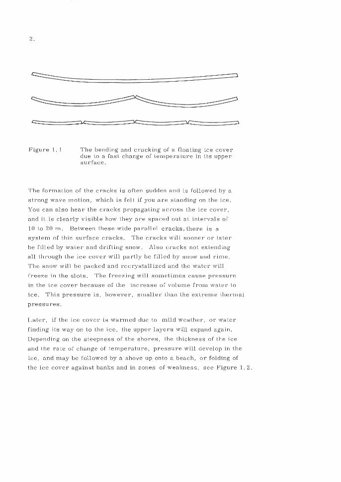
Figure 1.1 The bending and cracking of a floating ice cover due to a fast change of temperature in its upper surface.
The formation of the cracks is often sudden and is followed by a
strong wave motion, which is felt if you are standing on the ice.
You can also hear the cracks propagating across the ice cover,
and it is clearly visible how they are spaced out at intervals of
10 to 20 m. Between these wide parallel cracks, there is a
system of thin surface cracks. The cracks will sooner or later
be filled by water and drifting snow. Also cracks not extending
all through the ice cover will partly be filled snow and rime.
The snow will be packed and recrystallized and the water will
freeze in the slots. The freezing will someUmes cause pressure
in the ice cover because of the increase of volume from water to
ice. This pressure is, however, smaller than the extreme thermal
pressures.
Later, if the ice cover is warmed due to mild weather, or water
finding its way on to the ice, the upper layers will expand again.
Depending on the steepness of the shores, the thickness of the ice
and the rate of change of temperature, pressure will develop in the
ice, and may be followed by a shove up onto a beach, or folding of
the ice cover against banks and in zones of weakness, see Figure 1.2.

Figure 1.2 Examples of fJUHUl.Lii>=', ice covers
a) shoving up onto a beach b) out on a lake c) at a shore.
The magnitude of the ice pressure in the ice cover depends on
the rate of change of temperature in the ice, the coefficient of
thermal expansion, the rheology of ice, the extent to which the
cracks have been filled, the thickness of the ice cover, and the
degree of restriction from the shores.
Of course, the rate of change of temperature in an ice cover de
pends on the change of weather conditions such as wind speed, air
temperature, solar radiation, and the depth of the snow cover.
Expected of ice pressures due to thermal expansion at
a certain lake is thus obviously a function not only of ice and snow
properties but also of the local climate, ice conditions and lake con
figuration.
This study deals with those physical and mechanical properties of
ice that should be considered when calculating thermal ice pressures
in fresh or saline ice. Techniques to calculate pressures are
taken up in another study, "Thermal Ice Pressure in Lake Ice
Covers" (Bergdahl 1978) which demonstrates how this is done
for defined ambient conditions. Calculated values for five lakes
in Sweden between the latitudes 57°18' Nand 68 0 19'N are presented
in a third study, "Calculated and Expected Thermal Ice Pressures
in Five Swedish Lakes 11 (Bergdahl and Wernersson 1977).
3.
4.
1.2 Processes
A survey of the different processes considered when calculating
ice pressures due to the thermal expansion of an ice cover is given
below.
Thermal diffusion
Internal
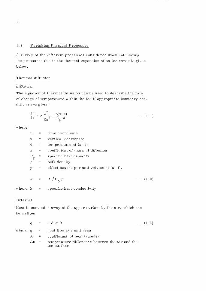
The equation of thermal diffusion can be used to describe the rate
of change of temperature within the ice if appropriate boundary con
ditions are given.
where
a8 at
2 a ~ + p(x, t)
C\ 2 C p ux p
time coordinate
x vertical coordinate
8 temperature at (x, t)
a coefficient of thermal diffusion
Cp specific heat capacity
p bulk density
p effect source per unit volume at (x, t).
a
where X specific heat conductivity
External
· .. (1. 1)
· .. (1. 2)
Heat is convected away at the upper surface by the air, which can
be written
q
where q
A
68
-A 6 8
heat flow per unit area
coefficient of heat transfer
· .. (1. 3)
temperature difference between the air and the ice surface
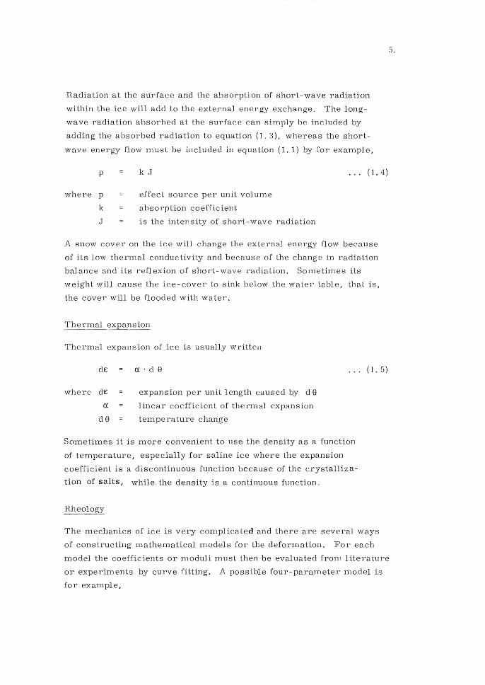
Radiation at the surface and the absorption of short-wave radiation
within the ice will add to the external energy exchange. The long
wave radiation absorbed at the surface can simply be included by
adding the absorbed radiation to equation (1 . 3), whereas the short
wave energy flow must be included in equation (1. 1) by for example,
p
where p
k
J
k J
effect source per unit volume
absorption coefficient
is the intensity of short-wave radiation
... (1. 4)
A snow cover on the ice will change the external energy flow because
of its low thermal conductivity and because of the change in radiation
balance and its reflexion of short-wave radiation. Sometimes its
weight will cause the ice-cover to sink below the water table, that is,
the cover will be flooded with water.
Thermal
Thermal expansion of ice is usually written
dE
where dE
r:J.
de
ex. • d 9
expansion per unit length caused by de
linear coefficient of thermal expansion
temperature change
... (1. 5)
Sometimes it is more convenient to use the density as a function
of temperature, especially for saline ice where the expansion
coefficient is a discontinuous function because of the crystalliza
tion of salts s while the density is a continuous function.
Rheology
The mechanics of ice is very complicated and there are several ways
5.
of constructing mathematical models for the deformation. For each
model the coefficients or moduli must then be evaluated from literature
or experiments by curve fitting. A possible four-parameter model is
for example,

6.
E () + K D ( G / E)n . .. (]. 6)
where t. rate of deformation, de.. /dt
stress rate, d er /di G
E modulus of elasticity
K, n coefficients for viscous deformation
D self diffusion coefficient for the molecul es in ice
all parameters above are functions of ice type and tempe
rature. The absorption coefficient and radiation balance are
functions of wave -1 ength too. The coefficient of heat transfer is
a [unction of wind - speed and humidity.
2. STRUCTURE OF ICE
One of the keys to the proper understanding of many ice problems
is the crystallography of ice. Its rheology, the scatter in strength,
values, the structure of sea ice and the shape of snowflakes can, for
example hardly be explained without some insight into the molecular
structure of the substance of water. Most of the information in this
chapter is taken from Pounder (1965)., Hobbs (1974) and Lavrov (1969).
2. 1 Substance of Water
As water is one of the most abundant substances on the surface of the
earth it has always fascinated men. Although it has a simple chemical
formula it has proved to behave anomalous in many ways. It has for
example extremely high specific heat capacity and specific latent
heat of fusion, its permittivity is abnormally high, and it shows an
inc rease in density when the temperature rises from 0 to + 4 0 C.
The chemical formula of water is mostly written H2 0 although in
liquid form water mostly appears as groups of molecules, polymers,
and thus could be desc ribed better by (H20)n where n is of the order
of ten. In the vapour state water exists as a monomer (H2 0)1 though
many dimers (H2 0)2 still do exist. Natural ice, on the other hand,
is crystalline, that is, the molecules are ordered in a regular space
lattice.
In the modern theory of valence the water molecule is viewed as
consisting of three nuclei su rrounded by ten electrons (Hobbs 1974).
Two of these electrons circle in the 1 s shell around the oxygen
nucleus, and the remaining eight electrons are in pairs occupying
four orbitals with mjxed sand p characteristics. Two of the or
bitals are the bonding orbitals directed towards the hydrogen nuclei,
the other two orbitals are called the lone-pair orbitals and point in
the opposite direction. The four orbitals form a roughly tetrahedral
system as is sketched in Figure 2. 1.
7.
8.
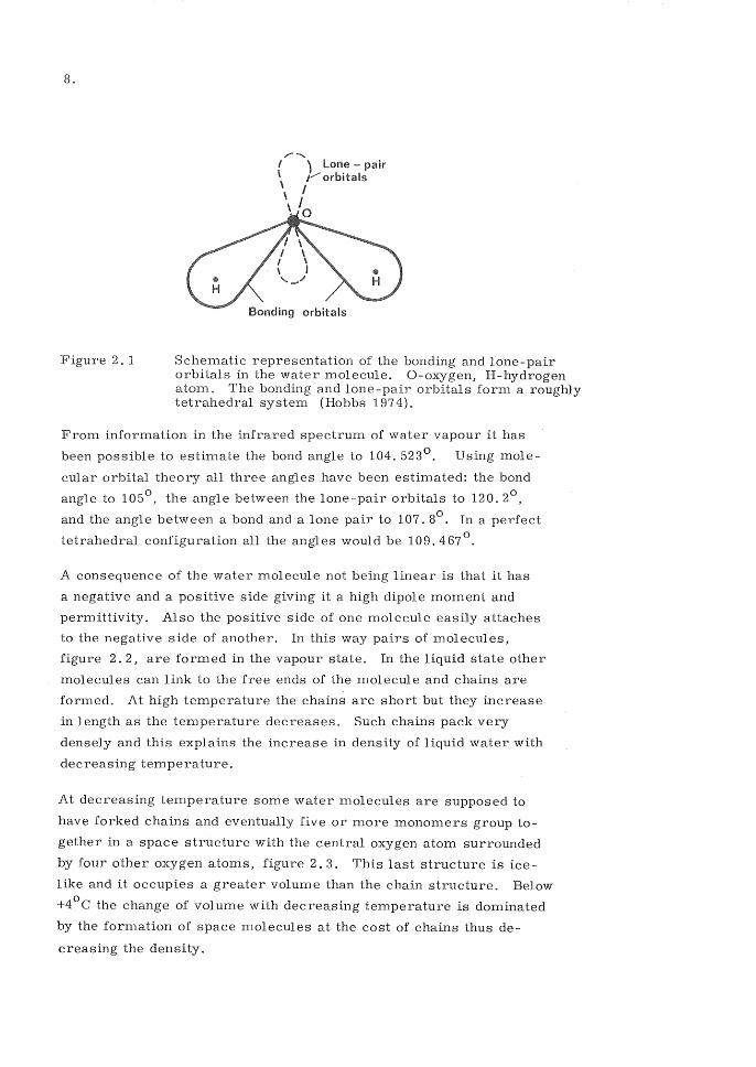
Figure 2. 1 Schematic representation of the bonding and lone-pair orbitals in the water molecule. O-oxygen, H-hydrogen atom. The bonding and lone-pair orbitals form a roughly tetrahedral system (Hobbs 1974).
From information in the infrared spectrum of water vapour it has
been possible to estimate the bond angle to 104.523 0. Using mole
cular orbital theory all three angles have been estimated: the bond
angle to 1050, the angle between the lone-pair orbitals to 120.2 0
,
and the angle between a bond and a lone pair to 107. 80• In a perfect
tetrahedral configuration all the angles would be 109.467 0•
A consequence of the water molecule not being linear is that it has
a negative and a positive side giving it a high dipole moment and
permittivity. Also the positive side of one molecule easily attaches
to the negative side of another. In this way pairs of molecules,
figure 2.2, are formed in the vapour state. In the liquid state other
molecules can link to the free ends of the molecule and chains are
formed. At high temperature the chains are short but they increase
in length as the temperature decreases. Such chains pack very
densely and this explains the increase in density of liquid water with
decreasing temperature.
At decreasing temperature some water molecules are supposed to
have forked chains and eventually five or more monomers group to
gether in a space structure with the central oxygen atom surrounded
by four other oxygen atoms, figure 2. 3. This last structure is ice
like and it occupies a greater volume than the chain structure. Below
+40
C the change of volume with decreasing temperature is dominated
by the formation of space molecules at the cost of chains thus de
creasing the density.
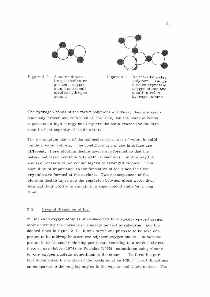
Figure 2. 2 A water dim er. Large circles represent oxygen atom s and small circles hydrogen atoms.
9.
Figure 2.3 An ice-like water polymer. Lar ge circles represent oxygen atoms and small circles hydrogen atoms.
The hydrogen bonds of the water polymers are weak, they are spon
taneously broken and reformed all the time, but the mass of bonds
represents a high energy and they are the main reason for the high
specific heat capacity of liquid water.
The description above of the molecular structure of water is valid
inside a water volume. The conditions at a phase interface are
different. Here electric double layers are formed so that the
outermost layer contains only water monomers. In this way the
surface consists of molecular layers of arranged dipoles. This
should be of importance to the formation of ice since the first
crystals are formed at the surface. Two consequences of the
electric double layer are the repulsion between close water drop
lets and their ability to remain in a supercooled state for a long
time.
2.2 Structure of Ice
In ice each oxygen atom is surrounded by four equally spaced oxygen
atoms form ing the corners of a nearly perfect tetrahedron, see the
dashed lines in figure 2.4. It will serve our purpose to believe one
proton to be midway between two adjacent oxygen nuclei. In fact the
proton is continuously shifting positions according to a more elaborate
theory, see Hobbs (1974) or Pounder (l965), sometimes being closer
to one oxygen nucleus sometimes to the other. To form the per-
fect tetrahedron the angles of the bonds must be 109.50 in all directions
as compared to the varying angles in the vapour and liquid states. The
10.
three lowest oxygen atoms in figure 2. 4 form an equilateral triangle
which makes a part of a so called basal plane.
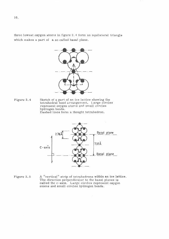
Figure 2.4
Figure 2.5
Sketch of a part of an ice lattice showing the tetrahedral bond arrangement. Large circles represent oxygen atoms and small circles hydrogen bonds. Dashed lines form a thought tetrahedron.
7.37 A c-axTs
A "vertical ll strip of tetrahedrons within an ice lattice. The direction perpendicular to the basal planes is called the c-axis. Large circles represent oxygen atoms and small circles hydrogen bonds.

Starting with the group of molecules forming the tetrahedron we can
expand the lattice' 'vertically" as is shown in figure 2. 5. There it
can be seen that its pattern is repeated a,t set distances, and that the
water molecules are concentrated to certain layers, the basal planes.
If the length of the bonds are 2. 76 A the distance between the basal
planes is calculated to 7.37 A.
A composition of the tetrahedrons in a "horizontal" plane, the upper
part of one of the basal planes in figure 2.5, for example, will result
11.
in the hexagonal pattern showing in figure 2. 6. This hexagonal symmetry
is reflected in the shape of snow flakes and ice particles. In the rime
on a window pane this pattern can be observed by anybody. The first
ice crystals forming at the surface of freezing water and etchings in
a polished ice surface also show their hexagonal character distinctly
(Hobbs 1974).
Figure 2.6
.. 4.52 A
A basal plane of ice. Observe that the corners of the hexagons are not on exactly the same level. The shaded group of molecules could be the lowest group in figure 2. 5. The diamond is a thought base of a unit prism. Large circles represent oxygen atoms and small circles hydrogen bonds.
The built-up ice crystal has only one axis of symmetry, the c-axis
or optical axis, which is perpendicular to the basal planes. Thus
ice would be expected to show anisotropy of physical properties.
An example of such an anisotropy is that slippage in ice occurs
most readily parallel to the basal planes. Slippage along other
planes demands stresses that are a magnitude greater. According
to Krausz (1968), the basal glide constitutes the main part of
12.
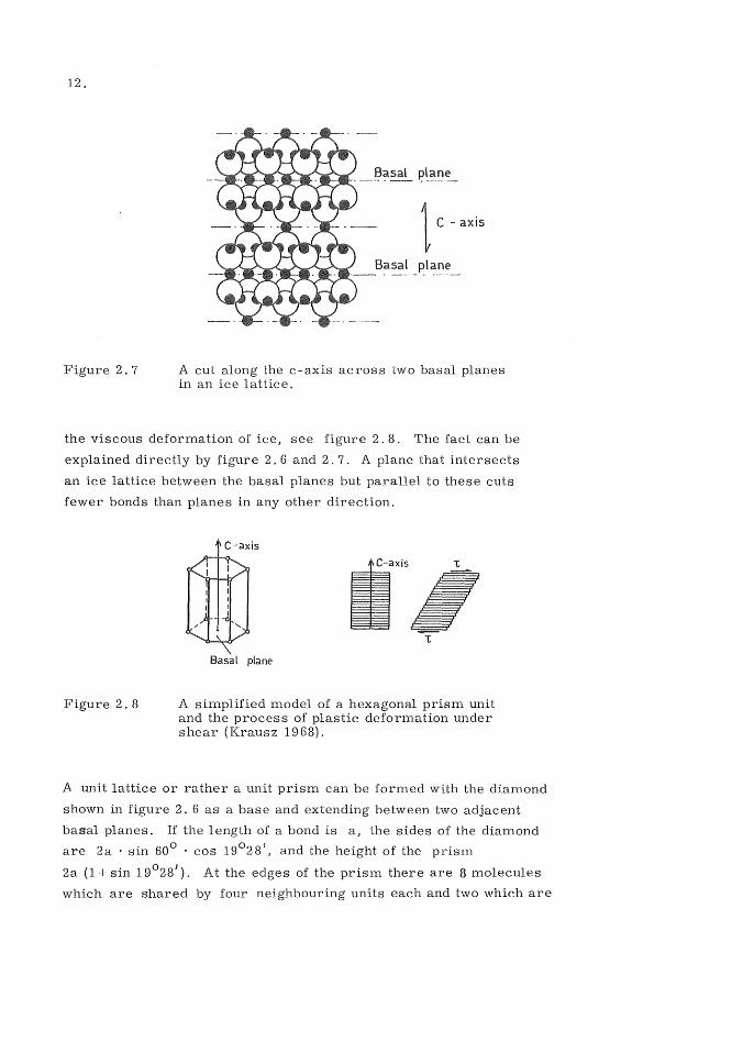
Figure 2.7
axis
Basal plane -_. --~-. --
A cut along the c-axis across two basal planes in an ice lattice.
the viscous deformation of ice, see figure 2.8. The fact can be
explained directly by figure 2. 6 and 2.7. A plane that intersects
an ice lattice between the basal planes but parallel to these cuts
fewer bonds than planes in any other direction.
Figure 2.8
C -axis
Basal plane
A simplified model of a hexagonal prism unit and the process of plastic deformation under shear (Krausz 1968).
A unit lattice or rather a unit prism can be formed with the diamond
shown in figure 2. 6 as a base and extending between two adjacent
basal planes. If the length of a bond is a, the sides of the diamond
are 2a' sin 60 0 • cos 19 0 28', and the height of the prism
2a (1 + sin 19 0 28'). At the edges of the prism there are 8 molecules
which are shared by four neighbouring units each and two which are
wholly within the unit. That is, four water molecules per unit the
mass of which is 4.2.992.10- 26 kg. The volume is then 3 . 3 0 2" 0 '(" . 0 I 8 a sm 60 cos 19 28 1 + SIn 19 28 ).
Finally the density is
p ... (2. 1)
and if at OOe p = 916.8 kg/m3 (Butkovich 1955), the bond length is o -10
calculated to 2.76 A (2.76 ·10 m) and the sides of the diamond
are 4. 52 A and the distance between the basal planes 7. 37 A.
Distances between points in a crystal, from where the lattice pattern
is identical, are sometimes referred to as Burgers vectors. In ice
there are thus two Burgers vectors namely 4.52 A and 7.37 A. The
notion is used within the theory of dislocations.
Other forms of solid H2
0 do exist as for example a variant with a
cubic lattice observed in experiments below _80oe. None of these
ice forms can exist at temperatures and pressures naturally occuring
on earth. They are stable only at pressures exceeding 0.2 GPa
(2000 bar) and therefore they are of no practical interest. See for
example Hobbs (1974) for a phase diagram of ice-water.
A crystal lattice is never perfect but contains defects of different
types. They may be inclusions of suspended or dissolved impurities
as for example salts or air molecules. Other defects are holes, that
is, missing atoms, and dislocations, that is, basal planes suddenly
interrupted or distorted. The dislocations has recently become of
greater interest as they form the basis of a modern theory of deform
ation and strength of materials. In figure 2. 9 two simple types of
dislocations are sketched. Lavrov (1969) discusses the most frequent
lattice defects in ice. The ice lattice is very selective and it accepts
no substitutes for oxygen or hydrogen with the exception of the fl uorine
ion.
13.
14.
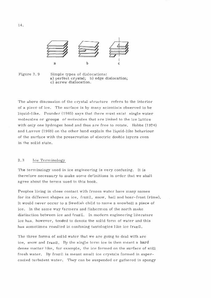
Figure 2.9
b c
Simple types of dislocations: a) perfect crystal; b) edge dislocation; c) screw dislocation.
The above discussion of the crystal structure refers to the interior
of a piece of ice. The surface is by many scientists observed to be
liquid-like. Pounder (1965) says that there must exist single water
molecules or groups of molecules that are linked to the ice lattice
with only one hydrogen bond and thus are free to rotate. Hobbs (1974)
and Lavrov (1969) on the other hand explain the liquid-like behaviour
of the surface with the preservation of electric double layers even
bl the solid state.
The terminology used in ice engineering is very confusing. It is
therefore necessary to make some definitions in order that we shall
agree about the terms used in this book.
Peoples living in close contact with frozen water have many names
for its different shapes as ice, frazil, snow, hail and hoar-frost (rime).
It would never occur to a Swedish child to name a snowball a piece of
ice. In the same way farmers and fishermen of the north make
distinction between ice and frazil. In modern engineering literature
ice has, however, tended to denote the solid form of water and this
has som etimes resulted in confusing tautologies like ice fraz il.
The three forms of solid water that we are going to deal with are
ice, snow and frazil. By the single term ice is then meant a hard
dense matter like, for example, the ice formed on the surface of still
fresh water. By frazil is meant small ice crystals formed in super
cooled turbulent water. They can be suspended or gathered in spongy
masses. By snow is meant precipitation in the form of airy crystals
depositing loosely and thus forming a layer with very low density.
Ice is often classified according to its genesis. Clear ice is for
example formed in a melt of liquid water. The clear ice can further
be classified according to crystal shapes and crystal axis orientation.
Snow ice is formed from a mixture of snow and water, frazil ice from
frazil and water et~. Sometimes also a classification according to
15.
the place, where the ice is found, is used. This is not recommendable.
Another very important classification is according to the salinity of
the ice into fresh-water ice and sea ice. The term sea ice is not
well chosen because it may include all types of ice at sea, for example,
ice bergs which have no salinity. A bette r choice of words would be
fresh-water ice and saline ice.
Michel and Ramseier (1971) have proposed a "Classification of River
and Lake Ice Based on Its Genesis, Structure and Texture". Their
classification, but not always their terms and explanations, will be
used in this book, when possible, and their notations PI, SI etc. will
be given below in connection with the description of different types
of fresh-water ice.
Other works on ice terminology are a working document by IAHR
(Kivisild 1970), International Glossary of Hydrology (WMO 1974),
WMO Sea Ice Nomenclature (1970), Illustrated Glossary of Snow
and Ice (Armstrong, Roberts, Swithinbank 1966), The Baltic Sea Ice
Code (1959), and a draft on Nordic ice terms (Fremling 1975).
2.4 Fresh-Water Ice
Fresh-water ice appears in a few varieties which have different
physical properties due to how they were formed. Some of the
properties can be explained by the size and shape of crystals other
properties by crystal axis orientation. To give some insight, the
process of ice-cover formation will be described below.

16.
2.41 Formation of Columnar Ice
When a lake is cooled down in the autumn the whole body of water
first attains the temperature +4 0 C which is the temperature of maxi
mum density of water. During this process the water of the lake
mixes easily in the vertical direction and the process is called the
autumnal turn-over. As the lake is cooled further the cooled water
stays at the surface because of the decreasing density. At calm
weather the surface layer rather fast reaches the freezing point
while the water at the bottom still can be +4 0 Co
The freeze-up happens mostly a clear and cold night and starts by
the growth of ice needles from nuclei of crystallization on the sur
face of the lake. The nuclei are often small hoar-frost crystals
precipitating from the cold air above the water surface. They can
be minute discoids or needles. The growing crystals first form
a sparse net and thereafter the meshes are grown over by thin clear
ice.
When the surface has been frozen over the ice cover increases in
thickness by the downward growth of the initial ice crystals, and
some of the crystals also grow horizontally at the cost of others.
The result of the ice-cover formation is columnar ice with oblong
crystals standing in the ice. Many of the crystals at the ice-water
interface are extended all through the ice cover, figure 2. 10. Their
length thus equals the thickness of the ice cover, and their diameter
increases with depth. At a depth of O. 3 to O. 6 m the diameter is
frequently 0.05 - 0.15 m.
Figure 2. 10
I ~ \ I IjfV \ l\f J)VY' ~l '\ r , / ~ Y / \
\ V
If I ( I
\ \ I
\ \ I
A vertical section through columnar ice with drawn crystal boundaries. As some crystals with favourable crystal-axis orientation encroach on others there are fewer but courser crystals at the underside of the ice cover.

The formed ice is called clear ice because of its transparancy, black
ice because it looks dark from above or columnar ice because of its
structure. Impurities in the water are concentrated at the crystal
boundaries, and in the spring when the ice is warmed by the sun most
of the radiation is absorbed in the crystal boundaries causing the
melting to start there. Shortly before the break up, the ice cover
therefore has deteriorated to densely packed but loosely connected
candle-like ice crystals. Such ice is called candIed ice.
At windy weather the initially formed ice consists of frazil or small
discoid crystals which form slush at the surface. This situation is
rather unusual, however, as generally a strong wind brings up warm
water from deep layers in the lake. Sometim es the lake is also
snown over before it has frozen, and the initial ice is then, of course,
formed from snow slush. When the slush has frozen the increase in
thickness proceed by the growth of the crystals down through the water
as described above.
2.42
The crystal-axis orientation in a columnar ice cover is important
to know because the rheological properties in c-axis direction are
different to those along the basal plane. As an example slippage in
ice crystals mostly occurs in the basal planes, figure 2.8.
The size of the crystals also influence the mechanical properties as
many crystal boundaries per unit volume give rise to more flexible
ice than few boundaries. In columnar ice horizontal c-axes imply
narrow crystals and vertical c-axes comparatively large crystals.
There has been a very long discussion on the reasons why there is
different crystal-axis orientation in lake ice covers. Sometimes
it has even been observed that one winter a whole lake ice cover has
mostly vertically oriented crystals, and the next winter on the same
lake there are mostly horizontally oriented crystals. Below is an
account for the results from this discussion, which explains seemingly
contradictory information on ice crystal orientation.
17.
18.
~~JE(~Yl ic~ y_l_C~I.E1_s.2!~~c~._ ~~my~r~~~e_gE:aj~l2..t J:n_tE:e_ ~a~eE::
The primary ice skin formed at the surface of a water reservoir or
lake at calm weather will either have randomly oriented crystals or
crystals with vertical c-axes. Vertical c-axes will dominate if there
is a temperature gradient in the water close to the surface because
nuclei with vertical axes will be able to grow fast over the cold surface,
while tilted nuclei cannot develop along their basal planes, because
these will tend to grow down into the warmer underlying water. Instead
the tilted crystals show up as long needles formed along the intersection
between their basal planes and the surface. The dominating vertically
oriented crystals are large (5-20 mm) to extra large (> 20 mm) and
it is not uncommon with giant (,-...J 1 m) crystals.
Random accis orientation in the primary ice skin will occur when there
is no thermal gradient in the water close to the surface. The nuclei
of crystallization can then develop in all directions and no crystals
are favoured. The crystal size ranges from medium (1- 5 mm) to
extra large (> 20 mm).
The description of the formation of the primary ice layer is in concord
with Shumskii (1955), Brill (1957), Hobbs (1974), Cherepanovand
Kamyashinkova (1971). Michel and Ramseier (1971) writes that the
rate of cooling or thermal gradient in the air influences the crystal
orientation, which it does only indirectly by creating either a gradient
in the water surface or a homogeneous supercooled layer of some
depth. The crystal size may however be influenced by the rate of
cooling. A high rate implies many nuclei per unit area while a low
rate implies relatively fewer.
~~im~rl ic~ ~ l ~~il2.. ~~z2J=-ice_c~v~r ~n.i ~ i ~~in snow-ic~ .£o~~r.:. If the freeze up starts in agitated water by the formation of frazil at
the surface or if the lake is snowed over, the primary ice layer will
of course have a random crystal orientation. The crystal size will
in both cases be fine « 1 mm) to medium (1- 5 mm), the shape
equiaxed, but the frazil-ice crystals will be angular while the snow-ice
crystals will be rounded.
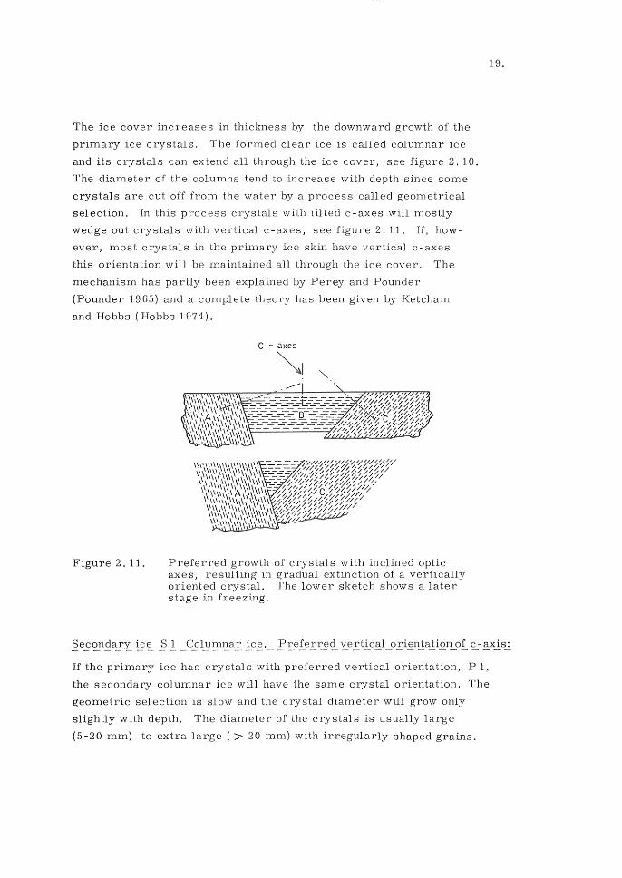
The ice cover increases in thickness by the downward growth of the
primary ice crystals. The formed clear ice is called columnar ice
and its crystals can extend all through the ice cover, see figure 2. 10.
The diameter of the columns tend to increase with depth since som e
crystals are cut off from the water by a process called geometrical
selection. In this process with tilted c-axes will mostly
wedge out crystals with vertical c-axes, see figure 2.11. If, how
ever, most crystals in the primary ice skin have vertical c-axes
this orientation will be maintained all through the ice cover. The
mechanism has partly been explained by Perey and Pounder
(Pounder 1965) and a complete theory has been given by Ketcham
and Hobbs (Hobbs 1974).
Figure 2. 11.
C - axes
~I
Preferred growth of crystals with inclined optic axes, resulting in gradual extinction of a vertically oriented crystal. The lower sketch shows a later stage in freezing.
If the primary ice has crystals with preferred vertical orientation, P 1 J
the secondary columnar ice will have the same crystal orientation. The
geometric selection is slow and the crystal diameter will grow only
slightly with depth. The diameter of the crystals is usually large
(5-20 mm) to extra large (> 20 mm) with irregularly shaped grains.
19.
20.
The length of crystals depends on the relative orientation of adjacent
crystals but can vary from large to the length equivalent to the thick
ness of the columnar ice layer. See figure 2. 10.
S 2 Columnar ice. Preferred horizontal orientation of c-axis:
If the primary ice has a random crystal orientation (types P2, P3 and P4)
the size of crystals will increase more rapidly with depth than for S 1.
The crystal orientation changes continuously with depth becoming pre
ferred horizontal after 5 to 20 cm of growth. The initial crystal size
would be the same as for the primary ice increasing to large (5-20 mm)
and possibly f'xtra large (». 20 mm) at the bottom of the columnar layer.
A lake ice cover can also contain other types of ice as for example in
perennially frozen arctic lakes where the columns can consist of giant
crystals with the c -axes horizontally and nearly parallel (S 3). When
ice is growing by crystallizing on an object or vertical ice surface the
c-axes will mostly be parallel to the surface. For example ice re
freezing in a bore hole will consist of needle -like crystals pointing at
the centre of the hole with their c-axes perpendicular to the needles.
In Sweden perennial ice is of no practical interest and the other type
of ice does not influence the over-all characteristics of an ice cover.
When making laboratory experiments it is often formed on the walls
of research basins which should be observed (Brill 1957, Muguruma
and Kikuchi 1963).
Most reports on the orientation of crystals in lake ice covers are
consistent with the account above as for examples descriptions given
by Knight (1963) or wind tunnel experiments made by Lyons and Stoyber
(1963). The latter scientists found that vertical c-axes dominated when
the wind speed was less than 1. 5 mls and at 2.7 mls horizontal axes.
Sometimes a thin ice consistuded by vertically oriented crystals may be
broken up into sInall discoids by a strong wind. The discoids are then
pushed together and made to tilt by the wind so that an ice cover with
mainly horizontal oriented ice of a crystal size of the order of 0.01 cm
is formed.
Also the observations by Muguruma and Kikuchi (1963) on Peter" s
Lake, Alaska, agree with the description above. They suggest that
at normal weather conditions ice with horizontal c-axes is formed and
that vertically oriented ice is formed when the wind breaks such thin
21.
ice and pushes it together. By normal weather they mean windy weather.
2.43 Frazil and Frazil Ice
When the turbulence in the water is too intensive the formation of a
surface ice sheet is prevented, and if the mass of water is supercooled
minute ice crystals form at the surface but swirl down and become
suspended. This is particular common in rapids, but can also be ob
served in waves, especially on shores and in shallow areas. The
formed crystals grow from colloidal particles to small discoids and
spikes that cluster together to porous aggregates. Such suspended
ice is called frazil.
In turbulent stretches anchor frazil is developed, that is, the frazil
sticks to stones or scraps on the bottom and also to the iron-parts
of intakes and turbomachinery. Sometimes it can clog a river or a
power-station very fast if the concentration of suspended frazil is
high. Motala Strom in Sweden is for example said to have flstopped
its pace 1708'1. The flow of that river is 42 m3/s. When going
full tilt, passing frazil and supercooled water through its turbines,
it can be a matter of seconds for a turbine to be completely choked
if the frazil starts to stick to the machinery. Another problem of
anchor frazil is that it can lift stones or scrap-iron from the bottom
and bring it into turbines or pumps where it damages the equipment.
Se~~n~a_I'Y.:0~ S i _Fr~z21 jc~: In river stretches with a low pace the
frazil flsediments" to the surface and forms frazil slush, eventually
stopped by some obstacle it may create a hanging dam. The mixture
of water and frazil is cooled from above and the water in the pores
freezes. A solid ice mass, frazil ice (S 4), is formed. The crystal
shape is equiaxed to tabular ranging from fine « 1 mm) to medium
(1-5 mm) sized. The crystal boundaries are irregular, and the
crystallographic orientation is random.
When investigating into the deformation and strength of ice as a mate
rial, it is often convenient to work with ice specimens that contains
22.
a lot of crystals, in order that the specimens be considered equal and
homogeneous. To this purpose frazil ice is well fitted. Manyexperi-
ments have also been done with artificial frazil ice made from saw dust
or splintered ice. See chapter 9: Mechanical Properties. In this respect
frazil ice is important, while it plays a minor role for thermal ice pressure.
2.44 Snow and Snow Ice
In connection to thermal ice pressure snow is of interest by two reasons.
First, because snow is a good insulator which effectively prevents
temperature variations in the air to reach the underlying ice or ground.
Secondly, because snow ice is very common on lakes in temperate areas,
why it is necessary to know the properties of snow ice as well as of
col umnar ice. The occurrence of natural snow ice is given in the next
paragraph 2.45. Below a very short summary of some features of
snow and hail is given. For an elaborate description of the precipitation
of snow it is referred to Hobbs (1974).
S now is formed in clouds by the crystallization of vapour on nuclei of
crystallization. The process results in light snowflakes. Hail, on the
other hand, is form ed by the collision of supercooled water droplets
that freezes when combining to bigger drops. This results in hailstones
or, if the original particles were snowflakes, in graupels. Raindrops
can also freeze and this results in ice pellets. Hailstones and graupels
are translucent or milky. Pellets are transparent. Ordinary snow
covers can, however, be considered to consist of only snow since hail
constitutes a very small fraction of the accumulated solid precipitation.
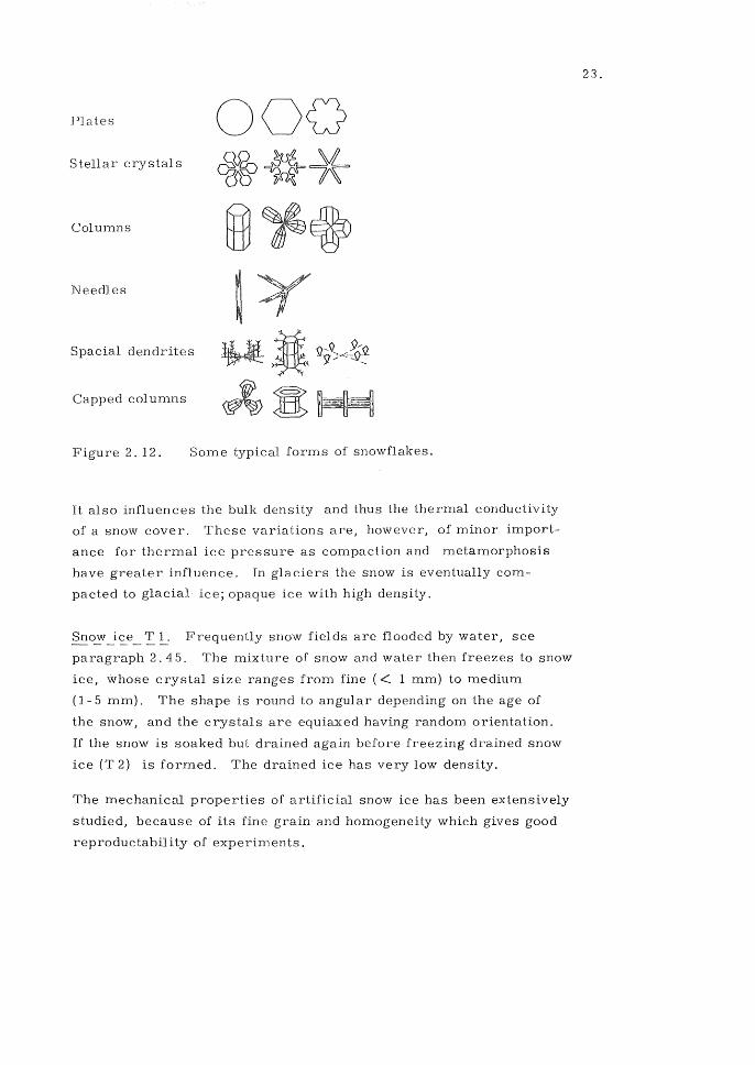
Snowflakes are hexagonal crystals and their shapes are legion. Some
typical shapes are hexagonal plates, six-pointed stellar crystals, solid
or hollow columns with hexagonal crossection, needles, spacial den
drites and capped columns see figure 2. 12. These basic shapes are
varied in innumerable ways and actually not two snowflakes are equal.
The basic forms of solid precipitation depend on the weather conditions,
and due to which form is most numerous the deposited snow cover
show different features. This is important for avalanche forecasting.
See for example Mellor (1965) or Seligman (1936).
Plates
Stellar crystals
Columns
Needles
Spacial dendrites
Capped columns
Figure 2.12. Some typical forms of snowflakes.
It also influences the bulk density and thus the thermal conductivity
of a snow cover. These variations are, however, of minor import
ance for thermal ice pressure as compaction and metamorphosis
have greater influence. In glaciers the snow is eventually com
pacted to glacial ice; opaque ice with high density.
Sno~ _i~e _ '!'.!.: Frequently snow fields are flooded by water, see
paragraph 2.45. The mixture of snow and water then freezes to snow
ice, whose crystal size ranges from fine (<. 1 mm) to medium
(1- 5 mm). The shape is round to angular depending on the age of
the snow, and the crystals are equiaxed having random orientation.
If the snow is soaked but drained again before freezing drained snow
ice (T 2) is formed. The drained ice has very low density.
The mechanical properties of artificial snow ice has been extensively
studied, because of its fine grain and homogeneity which gives good
reproductability of experiments.
23.
24.
2.45 Lake and River Ice Covers
Natural ice covers almost never have a simple structure, and have to
be very simplified to fit any mathematical model for calculation of
thermal pressures or even for simple observation purposes. Below
is a comprehensive review of the variations that can be expected,
freely after Fremling (a). See also Ager (1960), Lazier and Metge (1972).
On a lake the ice cover can be constituted (from top to bottom) by
snow, snow ice, slush and columnar ice. The snow can be moist and
compacted or dry and loose, the snow ice and slush can contain little
or lots of air, the columnar ice can show different crystal structure
as described earlier, and it can also hold various amounts of air
bubbles.
The ice cover also vary from place to place on the lake, for example
because of uneven accumulation of snow. At the inlet and outlet and
in straits the ice cover is affected by currents, and it may also be
flooded at the inlet. Along the shores the cover is bent and cracked
and sometimes flooded because of the rise and fall of the water level.
This is very pronounced in reservoirs especially if they are regulated
daily. To these variations comes thermal cracks and ice folds. Along
an ice fold the ice cover is treacherous with tilted ice blocks, newly
formed columnar ice, water, slush, and snow ice. In Sweden it is also
very common to plough winter roads on the ice which also causes
complications. Some winters a road for lorries has been prepared
across the Bothnian Bay between Sweden and Finland. The distance
is approximately 100 km.
The quality of the ice also varies with time. In early winter, when
there is little solar radiation the columnar ice is solid and strong.
In late winter the columnar ice is candIed by the sunshine, and although
it maintains its depth it consists largely of water and loose crystals.
On the other hand, if it is covered by snow or snow ice it is shielded
from the sun and will maintain its strength till the snow or snow ice
has disappeared. The snow ice is also affected by solar radiation so
that it melts at its crystal boundaries. The result of this is loose
granular ice (corn snow ice).

In rivers ice condition are still more complicated. In slow reaches
the conditions can resemble the conditions on a lake. In rapids and
narrow reaches, however, a lot of frazil ice is produced and carried
downstream creating hanging dams or accumulating as anchor frazil.
\;Vater levels will then rise and stretches of ice covers will lift from
its supports on the banks and shove onto each other, be broken into
pieces and eventually be carried downstream causing ice jams anew.
The water level will rise again and the process is restarted and will
go on till the river is completely ice covered, the runoff decreases,
25.
or the cold weather ceases. In spring the problems will start all over
and they are especially pronounced for rivers flowing into colder cli
mate as in the nothern Soviet- Union, Canada and Alaska. The problem
of thermal ice pressure is however of cOlY1paratively little importance
in such rivers. Uzuner and Kennedy (1974) have treated these problems
quantitatively. A description of the ice conditions in a Swedish un
regulated river, the Torne Alv, is given by 5MBI (1961).
The layers of snow slush and snow ice in the lake ice cover arise
because the ice is pressed down by the load from the snow. Water
will then find its way through cracks and holes up onto the ice cover
and it will usually rise capillary in the snow to a level higher than
the water table, thereby increasing the weight of the snow. The
sinking stops when the vertical equil ibrium is restored. See figure 2. 13.
Figure 2.13.
Dry snow j Capillary
I--_-_---_=-=:--::_=-=_=-=_-::_~=-=I
rise Dry snow
Water table
A vertical section through an ice cover before (a) and after (b) water has leaked onto it.
m
0 Torne trask I
Winter 1939/40 ~~I~~
Gautajaure
Winter
Vastra
Winter 1954/55
OCTOBER INOVEMBER I DECEMBER I JANUARY
Notations: ~ columnar ice
c=J snow
FEBRUARY I MARCH APRIL
f?/?}i/j slush
~ snow ice
0.6
0.8
1.0
0
0.2
0.4
0.6
0.8
0
0.2
0.4
~ MAY UUNE
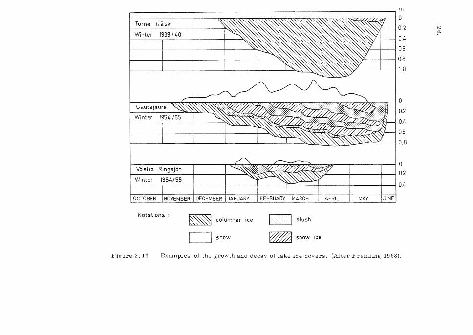
Figure 2.14 Examples of the growth and decay of lake ice covers. (After Fremling 1968).
rev ?J
The slush, that is, the mixture of water and snow, freezes to snow
ice from above and the columnar ice is warmed to OOC. After some
time the ice cover will thus be constituted by snow, snow ice, slush
and columnar ice. Often there can be several heavy snow falls in a
winter which creates an ice cover with repeated layers of snow ice
and slush.
Three examples of the growth and decay of lake ice covers are given
in figure 2.14. Torne Trask the winter of 1939/40 and Gautajaure
1954/55 are extreme examples of ice conditions. Torne Trask with
over 1 m solid columnar ice without snow and Gautajaure with three
double-layers of slush and snow ice on top of a rather thin (0.1 m)
columnar ice layer.
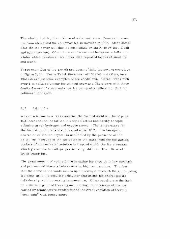
2. ;) Saline Ice
When ice forms in a weak solution the formed sol id will be of pure
H20 because the ice lattice is very selective and hardly accepts
substitutes for hydrogen and oxygen atoms. The temperature for
the formation of ice is also lowered under 00 C. The hexagonal
character of the ice crystal is unaffected by the presence of the
sal ts, but because of the exclusion of the salts from the ice lattice,
pockets of concentrated solution is trapped within the ice structure,
which gives rise to bulk properties very different from those of
fresh-water ice.
Tl-e great amount of void volume in saline ice show up in low strength
and pronounced viscous behaviour at a high temperature. The fact
27.
that the brine in the voids makes up closed systems with the surrounding
ice show up in the peculiar behaviour that saline ice decreases its
bulk density with increasing temperature. Other results are the lack
of a distinct point of freezing and melting, the drainage of the ice
caused by temperature gradients and the great variation of thermal
"constants" with temperature.
28.
Taking all these facts into account it is not easy to tell directly
how they will affect thermal ice pressure, although one astounding
conclusion can be drawn. In saline ice falling temperatures give
rise to pressures and rising temperatures will release the pressures.
This has been observed by Malmgren (1927). See e. g. Peschanskii (1971).
The magnitudes of the pressures are however difficult to judge. On
one hand the strong dependence of volume on temperature indicates
very big pressures, on the other hand the ice is a lot weaker than
fresh-water ice and the temperature response of the ice is a lot slower
because of the very high heat capacity.
2.51 Sea Water and Ice at Sea.
The salinity of sea water varies between 34 and 38 0/00 in the oceans.
In coastal areas and landlocked adjacent seas the variation can be
greater. However, the relative proportions of different salts are
nearly constant regardless of the absolute concentration. The major
constituents of the solution are listed in table 2.15. The concentrations
are expressed in kg per kg of solution, the total salinity in this example
being 34.48 0/00 , which is often taken as a standard figure. See for
example Dietrich and Kalle (1967). For the purpose of explaining
sea ice properties, it is enough to take the three major constituents
of table 2. J 5 into account.
Table 2.15. Composition of salts of sea water of the salinity 34.48 0/00
Salt NaCI MgC1 2 CaCl 2 KCl NaHC03
Other Total
23.48 4.98 3.92 1. 10 O. 66 0.19 0.15 34.48
It should be warned that the density of sea water and brine cannot be
directly expressed as the density of water plus the weight of the included
salts. See Chapter 3. 3 Density of Sea Ice. The reason for this is
that the ions affect the structure of the liquid water and also some
ions are hydrated. Another important effect is that standard sea
water does not have a point of maximum density and that the tempe-
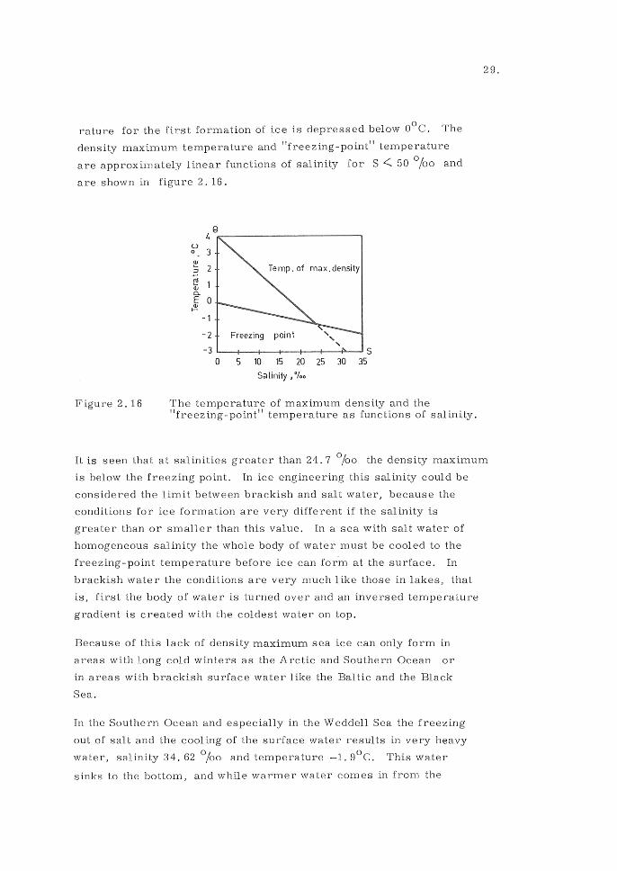
rature for the first formation of ice is depressed below oOe. The
density maximum temperature and "freezing-point" temperature
are approxim ately linear functions of salinity for S < 50 0/00 and
are shown in figure 2. 16.
Figure 2.16
e 4
u 0
QJ
~ Temp. of max.density en Q; Cl..
E QJ
0 I-
-1
-2 Freezing point
-3 S 0 5 10 15 20 25 30 35
Salinity 10/00
The temperature of maximum density and the "freezing-point" temperature as functions of salinity.
29.
It is seen that at salinities greater than 24.7 0/00 the density maximum
is below the freezing poi.nt. In ice engineering this salinity could be
considered the limit between brackish and salt water, because the
conditions for ice formation are very different if the salinity is
greater than or smaller than this value. In a sea with salt water of
homogeneous salinity the whole body of water must be cooled to the
freezing-point temperature before ice can form at the surface. In
brackish water the conditions are very much like those in lakes, that
is, first the body of water is turned over and an inversed temperature
gradient is created with the coldest water on top.
Because of this lack of density maximum sea ice can only form in
areas with long cold winters as the Arctic and Southern Ocean or
in areas with brackish surface water like the Bal tic and the Black
Sea.
In the Southern Ocean and especially in the Weddell Sea the freezing
out of salt and the cooling of the surface water results in very heavy
water, salinity 34.62 0/00 and temperature -1. 90 e. This water
sinks to the bottom, and while warmer water comes in from the
30.
north, the bottom water spreads to the north on the ocean floor. This
is actually part of the mechanism of ventilation of the world ocean.
The sinking water has a high content of oxygen and is fundamental
to the life in the sea. Other parts of the ocean playing the same
role but on a minor scale are the Sea of Okhotsk, the Greenland
and Irminger Seas (Dietrich and Kalle 1967).
In the southern part of Hudson Bay, in the Baltic and in the Black Sea
the top layer is brackish and consequently a cover of columnar ice
and snow is created ve ry much in the sam e way as in lakes.
In areas where big rivers flow directly into a cold saline sea, ice
is form ed at the interface between fresh and saline water. It is of
course continuously floating to the surface and can cause problem
to smaller vessels.
A lot of the ice in the seas of A rctic and Antarctic regions is of snow
origin. The ice bergs in the North Atlantic are calved from the gla
ciers of Greenland and Spitzbergen. The tabular ice bergs in the
Southern Ocean are broken off from the shelf ice surrounding the
Antarctic Continent. This glacial ice is, of course, of great im
portance to the life in the seas of the polar regions and is also a
problem to ships and off-shore installations but has little bearing
on thermal pressures
2.52 Formation of Columnar Sea Ice
When eventually ice forms at the sea surface it is growing in a deep
layer of water with its temperature at the freezing point and horno
geneous density. If considerable turbulence is present during freezing,
a layer of discoids and granular ice crystals are formed on the surface
as a slush. The slush may be several centimetres thick and it freezes
together to a fine grain « 1 mm) ice cover with randomly oriented
c-axes. This way of formation of the initial ice cover is frequent in
the sea. If the ice cover formation starts at a calm surface the
nuclei of crystallization grow to small disks and develop into dendritic
(ramified) stars. The crystal orientation in the latter case is pre
dominantly vertical.

As is the case in lakes, columnar ice is formed when the ice cover
is inc reasing its thickness. Crystals with horizon tal c -axes are
favoured but the process of geometrical selection (Chapter 2.42)
is much faster than in fresh water. It is in fact doubted that the
geometrical selection is responsible for the strong preference of
horizontally oriented crystals. It is for example observed by Lavrov
(1969) that if the initial ice skin has vertical c-axes, new crystals
with more favourable crystal orientation form spontaneously at the
interface. According to Pounder (1965) it is sufficient with 4 0/00
salinity to get a fast selection of crystals. Whatever the reason
all saline columnar ice has horizontal c-axes and a grain ranging
from fine « 1 mm) to large (5-20 mm). Very thick ice ( > 0.5 m)
can contain courser crystals in its lower layers.
Bennington (1963) discusses the reasons for crystal-axis orienta
tion in columnar sea ice thoroughly. The theories put forward are
based on the mechanical convection under the interface ice-water
and on the assumption of a gradient of supercooling put forward by
Shumskij.
Saline columnar ice is characterized by its great inclusions of brine
and air. \Veeks and As sur (1967) discuss this phenomenon in detail
and have also suggested a model for the shape of the voids and how
they vary with temperature. Their model will be accounted for be
low and used subsequently for the calculation of mechanical and
thermal properties. First, however, a qualitative description of the
formation of the columnar ice will be given.
As told above the crystal lattice itself is very selective, and there
fore the formed ice is pure ice, the salt remaining in the water. In
the growth front the salinity of the water increases in this way. As
the thickening of the ice cover continues the growing basal planes
stretch like plates or fingers down into the supercooled water and
not until their length is 2 to 3 cm, bridges are formed between the
plates. Brine is in this way confined in the ice. The brine voids
form vertical strings of beads in the ice cover. They are concentra
ted to certain basal planes at a distance of 0.5 to 0.6 mm, their dia
metre is approximately 0.05 mm, and their length approximately
3 cm.
:31.
32.
The salinity of the brine in the voids at the moment of confinement can
for sal t water be considered as equal to the salinity of the sea. The
enriched brine in the growth front is denser than the ambient water and
will therefore sink. In this way the salinity is kept constant at the inter
face. The brine in the narrow space between the platelets is, however,
slightly more concentrated and the faster the growth the higher the salin-
ity is in the formed brine voids. For brackish water the salinity at
the growth front must not necessarily be of the same salinity as the
ambient water, because brackish water can be stably layered over
colder but less salt water. Consequently the salinity in the brine voids
cannot be easily predicted. Still, columnar ice formed in salt water
is, of course, more saline than ice formed in brackish water.
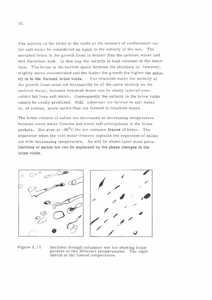
The brine volume of saline ice decreases at decreasing temperature
because more water freezes and more salt precipitates in the brine
pockets. But even at -80°C the ice contains traces of brine. The
expansion when the void water freezes explains the expansion of saline
ice with decreasing temperature. As will be shown later most pecu
liarities of saline ice can be explained by the phase changes in the
brine voids.
0 {}
f'
Figure 2.17
, /
/'
/ I
r~ /'
Sections through columnar sea ice showing brine pockets at two different temperatures. The right sketch at the lowest temperature.
A sea ice cover contains horizontal layers with greater concentrations
of brine voids and air bubbles, which form when the ice cover grows
uncommonly rapid. Other mechanisms tend to decrease the salinity
of the ice. One is that the brine voids move towards higher tempera
tures, that is mostly downwards. This fact will be explained in the
next paragraph. The draining off is amplified by gravitational
33.
drainage. Pounder (1965) says that the voids are interconnected at
temperatures over -15 0 C, which is contradictory to the fact that bulk
density changes actually obeys the theories founded on the assumption
of a closed system in the ice. The gradient drainage and possibly the
gravitational drainage add up so that winter ice has a typical salinity
of 4 0/00 and two year old ice of only 1 0/00 although the salinity of
newly formed ice can be as high as 20 0/00.
2.53 Phase Relations of Columnar Sea Ice
As is described in paragraph 2. 52 columnar sea ice will trap sea
water when growing. The trapped sea water brine is the cause of the
marked temperature dependence of many properties of columnar sea
ice. To calculate these variations as functions of temperature it is
necessary to take the phase changes of the two-phase system brine
and ice into account. (Assur 1958, Anderson 1960, Schwerdtfeger 1963,
Weeks 1963, Pounder 1965, Weeks and Assur 1967, Frankenstein and
Garner 1967).
A piece of sea ice with brine pockets can be regarded as a closed
system. For simplicity we disregard the existence of air-inclusions
in the ice. In such a closed system there is an equilibrium between
the brine and the frozen ice. In figure 2. 18 the "freezing-point curve"
of sea-water brine shows the concentration of brine in equilibrium
with ice at different temperatures. For example at -7. 60C, when
Na2S04 . 10 H20 starts to precipitate, the salinity of the brine at
equilibrium is approximately 110 0/00. That is, if the brine in the
pockets has a lower salinity, ice will form till the salinity of the brine
becomes 110 0/00. On the other hand, if the brine and ice is in equi
librium and the temperature is raised a couple of degrees ice will
melt from the walls of the pocket to dilute the brine until the new con
centration of equilibrium is reached. Due to gradients of concentration
near the walls of the pockets the response is slow in big pockets (Onu 1966).

34.
o 100 200 300 400
Concentration I % 0
Figure 2.18 "Freezing-point curve" of sea-water brine showing the concentration of brine in equilibrium with ice versus temperature. The various solid salts are listed opposite the segment of the curve in which they are the dominant salt crystallizing. Dashed lines indicate alternate interpretations, or possible alternate paths of crystallization (after Anderson 1960 with changes)
The curve, indicated kg salts /kg H 20 in figure 2.18, describes the
ratio between the mass of salts in solution and the mass of solvent
in the brine pockets as a function of temperature. This ratio is
piece by piece a linear function of tem perature which is convenient.
The relation between salinity S, mass of salts divided by mass of
solution, and the concentration s, mass of salts divided by mass of
solvent, can be written
s S / (1-S) or S s
1+8 ... (2.2)
Between 7. 60
C and the freezing point ef where no salts has preci
pitated the following equation holds
s = 0:. 1 e ... (2.3)
Between - 23 °c and -7. 6 0 C where Na 2SO 4 10 H20 gradually preci
pitates other equations must be formulated:
... (2.4)
Here p is the mass of precipitated salts divided by the mass of
solvent still in liquid form. According to Pounder (1965) o -1 0 -1 <Xl = - 0.01848 C and Cl
2 = - 0.01031 C .
Below - 23 0C there are alternate ways for crystallization
and several salts are gradually. The number of equa-
tions for the description of the
successively, but the
relations would thus increase
relations in the ice cause a
relatively small change in the bulk Y"Y''''~OY'Tl of sea ice below _23 0 C.
The reason is that at this low temperature the brine voids are rather
small. Equation(2. 4) will actually do for the calculation of the bulk
properties of columnar sea ice down to - 3 OOC, which is a very rare
temperature in ice covers whose undersides always are in contact
with liquid sea water.
The very first part of the "freezing- point 11 curve for salinity is in fact
the same as the curve of figure 2.16. For low salinity, that is the
salinity of ordinary sea water, this curve can also be considered
linear. Equation (2. 3) gives the freezing point for sea water as
8 =_s_= f Cl1
S < 0.050 ... (2.5)
Actually, there is no freezing point of sea ice in the ordinary sence
of the word, because at the so called freezing point ice only starts
to form and there is a gradual freezing of water in the ice as the tem
perature decreases. The heat of melting is in this way distributed
over a range of temperature so that there is no apparent latent
heat of freezing for the closed system but instead a very high specific
heat capacity. See chapter 4.
If an oblong brine void is situated along a stationary temperature
gradient according to figure 2.19 and the central part has a tempera
ture and salinity in equilibrium with the surrounding ice, the "cold"
and "warm" ends will not be in equilibrium. This is because the salt
diffuses in the void and so the salinity is nearly homogeneous. The
result is that water is freezing at the cold end and that ice is melting
at the warm end. This is one of the mechanisms by which already
formed ice looses salt.
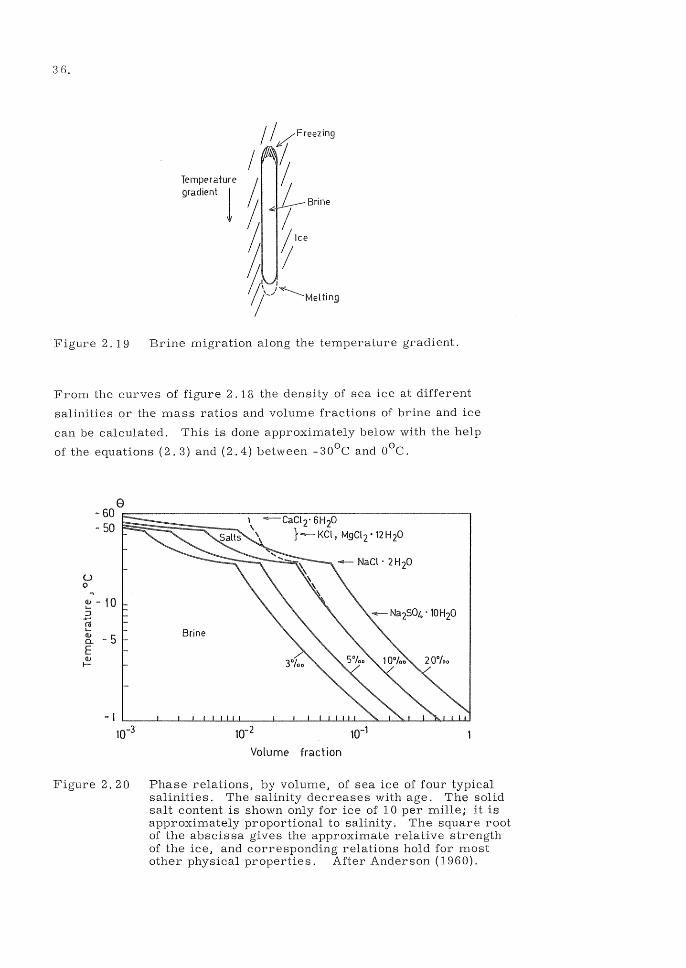
36,
/ / /Freezing
/ / Temperature / I gradient 1 / / /f
/ I /- Br;ne
I Jlce ~t t '1)--' "----Me I ti n B
Figure 2.19 Brine migration along the temperature gradient.
From the curves of figure 2,18 the density of sea ice at different
salinities or the mass ratios and volume fractions of brine and ice
can be calculated, This is done approximately below with the help
of the equations (2.3) and (2.4) between _30 oe and oOe.
u o
... ~ - 10 ;:J
~ ~ -5 E (); I-
Brine
-1 ~ __ -L __ L-L-~~~ ____ L--L-L~LLWW __ ~~~~~~~
10-3
Figure 2.20
10-2
Volume fraction
Phase relations, by volume, of sea ice of four typical salinities, The salinity decreases with age, The solid salt content is shown only for ice of 10 per mille; it is approximately proportional to salinity. The square root of the abscissa gives the approximate relative strength of the ice, and corresponding relations hold for most other physical properties. After Anderson (1960),

In figure 2. 20 the volume fraction of brine is drawn for some typical
salinities of sea ice. From this figure it can be seen that at _2 0 C
sea ice with a salinity of 20 0/00 is more than half liquid while at
_5 0 C the same ice is liquid only to 1/5 by volume. This has, of
course, a great influence on the strength of ice and we will look
closer at that in chapter 9.
The mass ratios of the phases of columnar sea ice as a function of
temperature 8 and ice salinity S was calculated by Schwerdtfeger
(1963) with the help of equation (2.2) to (2.4). The mass ratios are:
m. mass of ice (H20) to mass of the system 1
mb mass of brine 11
m mass of precipitated salts - 11 -P
The sum of the ratios is unity by definition.
o For -7. 6 C < e < Q f all the salt is in solution thus
37.
m i + mb . " (2.6)
and the salinity of brine Sb is given by
From equation (2. 2) then
sb S = 1 + sb . mb
from which the mass ratios mb and
m = b
m. = 1
Sb - ( 1 + sb) S 1 - mb = ---.,-----
m. 1
... (2.7)
... (2.8)
can be calculated
(2.9a)
... (2. 9b)
If the densities of brine and ice is known the volume fraction of
brine is -1
( 1 + ) mbP i
... (2.10)
38.
For _23 0 C < 8 < -7. 60 C a similar analysis can be made which
results in
m = b sb + P
m. 1-m-m 1 b P
sb +p - S {I + sb + p (3 )
p
... (2.l1a)
(2.11b)
... (2.11c)
(3 stands for the mass of the water of hydration in the precipitated
Na 2S04
. 10 H20, (3 2.27
The volume fraction of brine is consequently
... (2. 12)
Returning to the freezing point of sea water another interesting fact
can be demonstrated. Namely, if it is assumed that there is a free
exchange of water between the growing platelets and the sea under
neath} the salinity in the brine voids will be equal to the salinity of
the sea water Sa' The salinity of the formed ice will then be
S=s m a bo ... (2.13)
where m bo is the mass ratio of brine at trapping.
The freezing point is by equation (2. 5)
... (2.14)
but the melting point for the ice when it is no longer in contact with
the sea water will be higher namely
'" (2.15)
The fraction mbo cannot easily be predicted, but for very fast
freezing S can be as high as half the salinity of the ambient waten
so that the melting point becomes at least
... (2.16)
\iVith the aging of the ice there will be still lower salinity and the
melting point will be correspondingly raised. The high salinity
S 1/2 S also gives that mb according to (2.13) is as high as a 0
50 %.
The relations calculated in this paragraph will be used subsequently
to derive many properties of columnar sea ice, and it is important
to bear in mind the assumption that the ice was considered free of
air bubbles and that we also did not discuss the possibility that
vapour could exist in the system.
2.54 A Structural Model of Columnar Sea Ice
The complicated macrostructure of columnar sea ice, shown in
figure 2. 1 7, has been successfully conventionalized to a simple
pattern in order to describe the variation of strength with tempe
rature (Assur 1958) and for the calculation of thermal conductivity.
(Anderson 1960, Schwerdtfeger 1963)
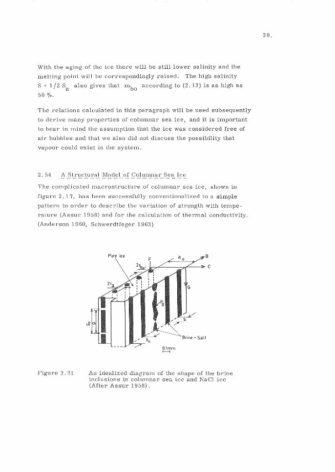
Figure 2.21 An idealized diagram of the shape of the brine inclusions in columnar sea ice and NaCl ice (After Assur 1958) .
39.
40.
Taking hold of the characteristic features of the brine inclusions in
columnar sea ice an idealized diagram can be made as that in figure
2.21. In the diagram the c-axis of the crystal is horizontal and the
G - axis is vertical. Different assurnptions of how the shape of the
brine voids change with brine volume can be made and will give dif
ferent relations between bulk properties and temperature. These
relations will be described in the chapters on thermal and mechanical
properties respectively, where the model will be used.
As mentioned earlier columnar sea ice also contains trapped air
bubbles, which are less orderly arranged, compared to the brine
voids. When calculating bulk properties of ice the air bubbles will
sometimes be taken into account and sometimes be disregarded.
The various excuses for this will be explained in due course. Here,
it should only be pointed out that stored specimens of saline ice might
have been drained off, especially, if they have been stored at an in
adequately high temperature. Such a mistake would, of course, offset
the intention to verify most of the theories founded on the salinity of
the ice, because the void volume of the ice will be related to the ori
ginal ice salinity and to the storing telnperature rather than to the
actual salinity of tested specimens.
2.55 Saline Snow Ice
Sea ice covers can be submerged by the load of deep snow in the same
way as lake ice covers, see paragraph 2.45. The result is saline
slush that freezes to a saline snow ice. This ice must, of course,
follow the same phase relations as described above for columnar sea
ice, but the distribution, shape and interconnection of the voids are
little discussed in literature, why it is difficult to quantify any of its
properties. Qualitatively it may be guess ed that its great content of
air makes it impossible to calculate its volume as a function of tem
perature.
Saline snow ice will not be discussed further in this book although it
is abundant in the Baltic for example. My knowledge of the subject
is simply too small.

3. DENSITY
The bulk density of natural ice is very variable due to inclusions of
air and brine. As its crystal lattice is very selective the bulk density
can,however,always be calculated by means of the densities of its
constituents, or rather its content of air and salt can be calculated
from measured bulk density values.
41.
The air inclusions in fresh water ice can make the ice at least 5 % easier than compact ice, but the air do not influence the thermal ex
pansion because the air bubbles are very soft compared to the surround
ing ice. For the calculation of thermal capacity and conductivity it
is, however, important to know the air content because in these respects
the air content cannot be neglected.
When calculating thermal expansion of saline ice, the density of the
trapped brine must be known. As the brine is enclosed in a
system, its density can be given at the equilibrium salinity for each
temperature, and thus the brine density in the brine voids is a function
of only temperature. An approximate polynomial is given in para
graph 3.31.
3. 1 of Pure Ice
The density of chemically pure ice without inclusions is usually given
as 916.8 kgjm3 at oOe, see for example Dorsey (1940). Butkovich
(1955) confirmed this by making very accurate measurements of single
crystals at 3. 50 e. He got the value 917.28 kgjm3 which extrapolated
to oOe by means of the coefficient of thermal expansion gives 916.82 kgjm3 .
Butkovich (1957) also measured the density as a function of temperature.
His experiments gave that the volume expansion with temperature is
linear with good accuracy between -30o e and oOe. Anderson (1960)
proposed a constant volume coefficient of thermal expansion y of
1. 445 . 10 -4 jK in this interval which gives good agreement also to
other scientists results. The volume coefficient, y , being three times
the linear coefficient, a, the latter amounts to 4. 82 . 10- 5 jK.
42.
The density as a function of temperature will be given by
p (8) = p / (1 + Y 8) o
... (3.1)
where p = 916.82 kg/m3 is t,he compact density of ice at OOC, p(8) the o
compact density at the temperature e, and y the volume coefficient of
thermal expansion.
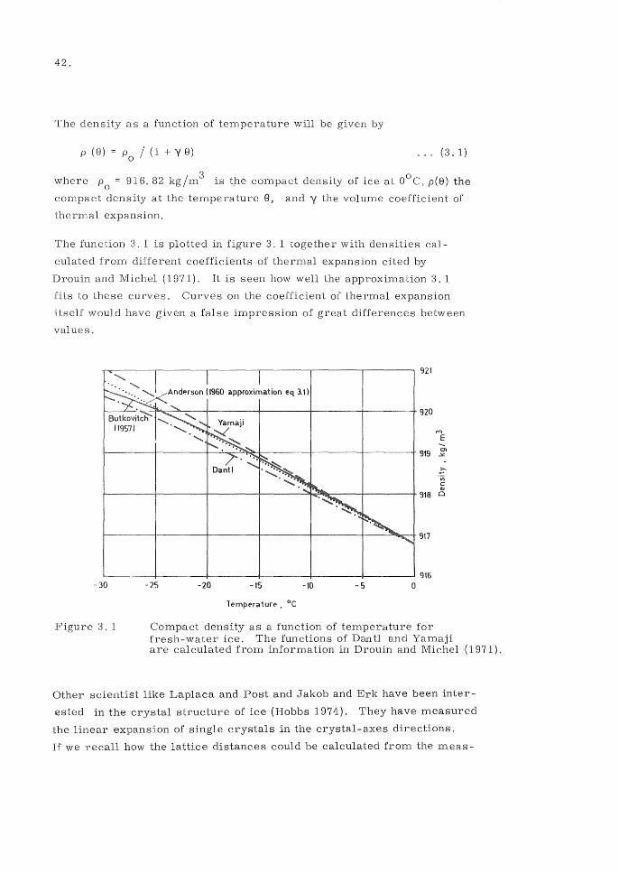
The function 3. 1 is plotted in figure 3. 1 together with densities cal
culated from different coefficients of thermal expansion cited by
Drouin and Michel (1971). It is seen how well the approximation 3.1
fits to these curves. Curves on the coefficient of thermal expansion
itself would have given a false impression of great differences between
values.
921
" -....... .' ....... )<And~rson (1%0 approximiition I:'q 3.1)
30
Figure 3. 1
920
M
E -919 t7I
..)C
::: 'iii c: Q1
918 0
917
916 -25 -20 -15 -10 -s 0
Compact density as a function of temperature for fresh-water ice. The functions of Dan tl and Yamaji are calculated from information in Drouin and Michel (1971).
Other scientist like Laplaca and Post and Jakob and Erk have been inter
ested in the crystal structure of ice (Hobbs 1974). They have measured
the linear expansion of single crystals in the crystal-axes directions.
If we recall how the lattice distances could be calculated from the meas-
43.
ured density of ice, we can imagine how changes of the distances be
tween the molecules in ice are reflected in a change of crystal dimen
sions. See chapter 2. 2. Ice crystals actually expands anisotropically
but in an ice cover the crystal orientation is irregular enough to cancel
out these differences.
Although the freezing of water to ice means an increase of volume of
9 this does not cause significant horizontal movements or loads in
an ice cover, because the increase in volume takes place in the direc
tion of heat transport. Janson (1963) verified this by freezing two open
wooden boxes full of water, one box insulated on bottom and walls the
other one uninsulated. The first box took a freezing to the bottom.
The walls of the other box burst apart.
Water freezing in cracks in the ice is, however, cooled by the surrounding
ice and therefore it expands sideways which gives rise to pressure. As
the cracks are only a small fraction of the area, the pressure will never
be of the same magnitude as extreme thermal pressures. 0.3 MPa
would be a common value.
The bulk density of natural fresh-water ice has been measured by for
example Ager (1963 a, b) in a cold room of a temperature of - 9.5 °C.
The specimens were weighed in air and the volume was measured by
submerging them in kerosene.
Naturally formed columnar ice (S1 or S2) was found to have a density
of between 870 and 920 kg/m3 . The density of ice formed from water
pumped onto a lake ice cover without snow in layers of 1- 5 cm was 3 found to vary between 870 - 910 kg/m .
Snow ice (T 1) formed by pumping or by natural flooding gave values
ranging from 870 - 910 kg/m 3
although most values was between 3 880 and 900 kg/m . If the water penetrates very slowly through the
snow cover and the snow has a fine grain, snow ice with a density as
low as 870 kg/m 3 can be formed.
If the snow is soaked by water but drained before freezing, the density
of the resulting ice (T 2) is of the order of 600 kg/m 3 (Michel and
Ramseier 1971).
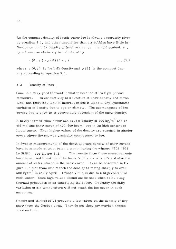
44.
As the compact density of fresh-water ice is always accurately given
by equation 3.1, and other impurities than air bubbles have little in
fluence on the bulk density of fresh-water ice, the void content, V ,
by volume can obviously be calculated by
p(8,v)=p(8)(1-V) ... (3.2)
where p (8, v) is the bulk density and p (8) is the compact den
sity according to equation 3.1.
3.2 of Snow
Snow is a very good thermal insulator because of its light porous
structure. Its conductivity is a function of snow density and struc-
ture, and therefore it is of interest to see if there is any systematic
variation of density due to age or climate. The submergence of ice
covers due to snow is of course also dependent of the snow density.
A newly formed snow cover can have a density of 100 kg/m 3 and an
old melting snow cover of 400- 600 kg/ m 3 due to its high content of
liquid water. Even higher values of the density are reached in glacier
areas where the snow is gradually compressed to ice.
In Sweden measurements of the depth average density of snow covers
have been made at least twice a month during the winters 1909 -1928
by 5MBI, see figure 3.2. The results from these measurements
have been used to estimate the loads from snow on roofs and also the
amount of water stored in the snow cover. It can be observed in fi
gure 3.2 thut from mid March the density is rising sharply to over
500 kg/m 3 in early April. Probably this is due to a high content of
melt water. Such high values should not be used when calculating
thermal pressures in an underlying ice cover. Probably the daily
variation of air temperature will not reach the ice cover in such
occasions.
Drouin and Michel (1971) presents a few values on the density of dry
snow from the Quebec area. They do not show any marked depend
ence on time.
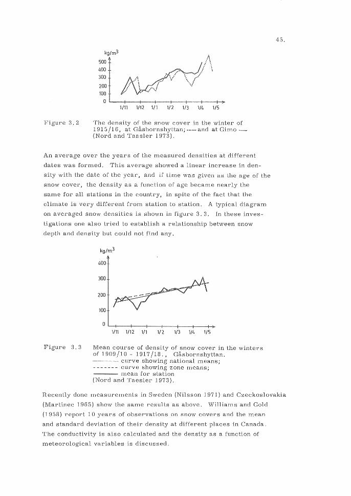
Figure 3.2
kg/m3
500
400 300
200
100
o ~--+----r---+----r---+----r---+~ 1/11 1/12 1/1 1/2 1/3 1/4 1/5
The density of the snow cover in the winter of 1915/16, at Gasbornshyttan; ...... and at Gimo (Nord and Taasler 1973).
An average over the years of the measured densities at different
dates was formed. This average showed a linear increase in den
sity with the date of the year. and if time was given as the age of the
snow cover, the density as a function of age became nearly the
same for all stations in the country, in spite of the fact that the
climate is very different from station to station. A typical diagram
on averaged snow densities is shown in figure 3.3. In these inves
tigations one also tried to establish a relationship between snow
depth and density but could not find any.
Figure 3.3
400
300
200
100
o ~+-__ ~ __ -+ __ ~~ __ +-__ ~ __ -+~ 1/11 1/12 1/1 1/2 1/3 1/4 1/5
Mean course of density of snow cover in the winters of 1909/10 - 1917/18., Gasbornshyttan. ----- curve showing national means; - - - - - - - curve showing zone means; ---- mean for station (Nord and Taesler 1973).
45.
Recently done measurements in Sweden (Nilsson 1971) and Czeckoslovakia
(Martinec 1965) show the same results as above. \Villiams and Gold
(1958) report 10 years of observations on snow covers and the mean
and standard deviation of their density at different places in Canada.
The conductivity is also calculated and the density as a function of
meteorological variables is discussed.
46.
Reasonable bulk densities for dry snow covers are 200 to 300 kg/m 3 .
The porosity of snow can, of course, be calculated by equation .3.2,
but the dependence on temperature can be neglected. Thus:
where V is the porosity of snow by volume
Po the compact density of ice at OoC
Ps the bulk density of snow
3. 3 of Sea Ice
... (3.3)
From the phase relations of saline ice the density of columnar sea
ice without air inclusions can be calculated. This has been done
by for example Riemer (see Kalle 1943), Anderson (1960) and
Schwerdtfeger (1963). The two former scientists results are
approximately the same. Schwerdtfeger has deduced a simple
analytical expression, but, unfortunately, working with an erroneous
expression for the brine density, his sea-ice density values are 2 % too small.
The theoretical values calculated from the phase relations show gen
eral agreement with the experimental data given by Petterson (in
Malmgren, 1927). It should be stressed that the densiti.es are assumed
to follow the volume variations of the components calculating with the
formation of neither voids nor internal pressures.
3. 31 §.e~::}~e _D~nslty- calc~l~tec!.J.£o.!? ~h~s~ lt~l~tlo~s_
For temperatures above -7.6 °c the following expression holds for
the density of columnar sea ice without air inclusions.
. .. (3.4)
o - 7.6 C ~ e ~ ef
where the weight ratios mb and m i are given by the equations 2. 9a
and b respectively, and the density of ice Pi = p( 8) by equation 3. 1 .

47.
The expression 3.4 was set up by Schwerdtfeger (1963) who, however,
used an uncorrect expression for the density of the brine namely
Pb = (1 + sb) Pw
where Pw is the density of pure water. An approxi
mate expression for the density at low salinities is Pb (1 + 0.7 Sb) Pw and as s /' S Schwerdtfeger' s expression for the brine density is
around 10 % wrong at 20°C, which is reflected as 2 % in the bulk
density of the ice.
A better fit to real values is given by the polynomial
Pb
( 8)= 999.9 - 16.04 8 0.520 82 - 0.00800 83
30°C'::::; 8 ~ oOe ... (3.5)
which gives the density of the brine correctly to within 4 % in the
interval _30oC~ 8 ~OoC. The polynomial is constructed from the
density values at 0, - 8, -16 and - 30°C, and is consequently correct
at these temperatures. The value at OOC is taken from I 'Kalle' s
tables", the others from Anderson (1960).
Observe that the density of the brine is a function of temperature H only.
This is due to the fact that it is the density at the equilibrium salin
ity for each temperature in the closed voids. The salinity of the brine
is thus implicitely given by the temperature and can be evaluated by,
for example, the curve of figure 2.18 .
For temperatures below -7. 60 C the density is given by the following
expression
p(8, S) = (mb/Pb + m /p + m./p.f1
p p 1 1
'" (3.6)
where the mass ratios of brine m b , precipitated salts mp' and
ice m i are given by the equations 2. 11, and the density Pp of the
precipitated salt Na 2S04 · 10 H20 is set to 1500 kg/m 3 according
to Anderson (1960).
Strictly the mass ratios of the equations 2.11 do not hold below 230
C,
but still the function 3.6 for the bulk density gives reasonably accurate
results, for the purpose of calculating thermal pressures, that is.
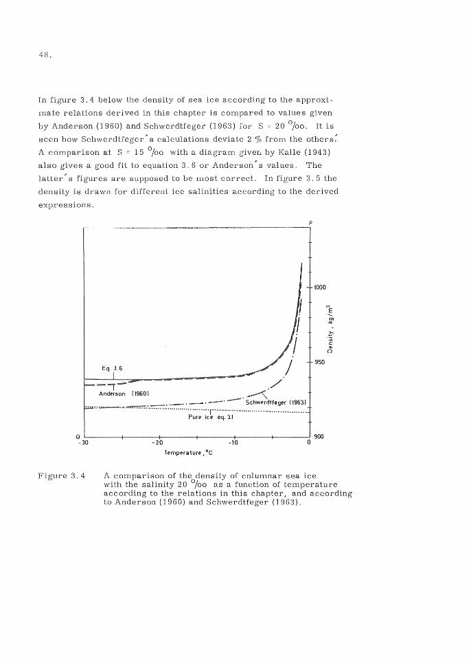
48.
In figure 3.4 below the density of sea ice according to the approxi
mate relations derived in this chapter is compared to values given
by Anderson (1960) and Schwerdtfeger (1963) for S = 20 0/00. It is
seen how Schwerdtfeger' s calculations deviate 2 % from the others~
A comparison at S = 15 0/00 with a diagram giveri by Kalle (1943)
also gives a good fit to equation 3. 6 or Anderson' s values. The
latter's figures are supposed to be most correct. In figure 3.5 the
density is drawn for different ice salinities according to the derived
expressions.
p
1000
950 Eq.3.6
,/ (1960) __ . ~ .
... ... ____ .. ,.~:.~.: ......... :.-.. -. _.-' Schwerdtftger (1963) •• .... t ...................... •• .. •• .. • .. •• .. • .... • .. •
PUft' ic t' eq. 3.1
e L-------+-------+-------~------1-------~------~ 900 - 30 20 -10 0
Figure 3.4
Tt'mperature .oc
A comparison of the density of columnar sea ice with the salinity 20 0/00 as a function of temperature according to the relations in this chapter, and according to Anderson (1960) and Schwerdtfeger (1963).
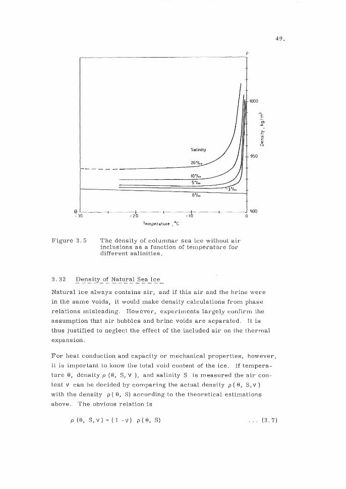
1000
950
8 ~------+-------+-------4-------~------~------~ 900 - 30 - 20 - 10 0
Figure 3.5 The density of columnar sea ice without air inclusions as a function of temperature for different salinities.
49.
E -.. Cl
.)(
.?:-'0; c Oil
0
Natural ice always contains air, and if this air and the brine were
in the same voids, it would make density calculations from phase
relations misleading. However, experiments largely confirm the
assumption that air bubbles and brine voids are separated. It is
thus justified to neglect the effect of the included air on the thermal
expansion.
For heat conduction and capacity or mechanical properties, however,
it is important to know the total void content of the ice. If tempera
ture e J density p (8, S, \I ), and salinity S is measured the air con
tent V can be decided by comparing the actual density p (8, S, V )
with the density p ( 8 J S) according to the theoretical estimations
above. The obvious relation is
p (8, S,V) = (1 V) p(8, S) ... (3.7)
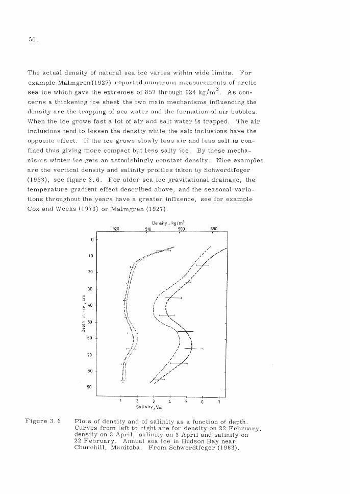
50.
The actual density of natural sea ice varies within wide limits. For
example Malmgren (1927) reported numerous measurements of arctic
sea ice which gave the extremes of 857 through 924 kg/m 3 . As con
cerns a thickening ice sheet the two main mechanisms influencing the
density are the trapping of sea water and the formation of air bubbles.
When the ice grows fast a lot of air and salt water is trapped. The air
inclusions tend to lessen the density while the salt inclusions have the
opposite effect. If the ice grows slowly less air and less salt is con
fined thus giving more compact byt less salty ice. By these mecha
nisms winter ice gets an astonishingly constant density. Nice examples
are the vertical density and salinity profiles taken by Schwerdtfeger
(1963), see figure 3.6. For older sea ice gravitational drainage, the
temperature gradient effect described above, and the seasonal varia
tions throughout the years have a greater influence, see for example
Cox and Weeks (1973) or Malmgren (1927).
Figure 3.6
10
20
30
E u
~ 40 .~
.c. 50 ~ o
60
70
80
90
920 Density, kg/m3
910 900
.. ::::: .. ::."." .. "~." 0/ j/
..;..;
!! 11
~~ 77
.... : ... rh!
n +~
Salinity J °/00
890
Plots of density and of salinity as a function of depth. Curves from left to right are for density on 22 February, density on 3 April, salinity on 3 April and salinity on 22 February. Annual sea ice in Hudson Bay near Churchill, Manitoba. From Schwerdtfeger (1963).
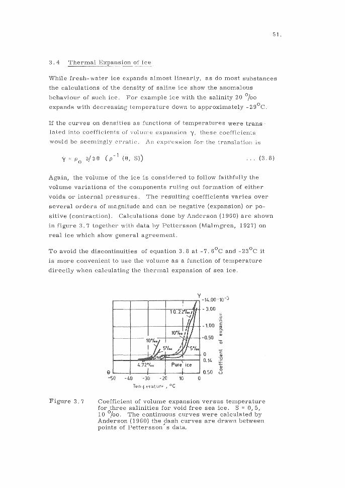
.51 .
3.4 Thermal of Ice
While fresh-water ice almost linearly, as do most substances
the calculations of the density of saline ice show the anomalous
behaviour of such ice. For example ice with the salinity 20 0/00
expands with decreasing temperature down to approximately 2 90 C.
If the curves on densities as functions of temperatures were trans
lated into coefficients of volU1lle expansion y, these coefficients
would be seemingly erratic An expression for the translation is
... (3.8)
Again, the volume of the ice is considered to follow faithfully the
volume variations of the cornponents ruling out formation of either
voids or internal pressures. The resulting coefficients varies over
several orders of magnitude and can be negative (expansion) or po
sitive (contraction). Calculations done by Anderson (J 960) are shown
in figure 3.7 together with data by Pettersson (Malmgren, 1927) on
real ice which show agreement.
To avoid the discontinuities of equation 3.8 at -7. 60 C and -23 0 C it
is more convenient to use the volume as a function of temperature
directly when calculating the thermal expansion of sea ice.
Figure 3.7
y -14.00 '10-3
- 3.00 c 0 'iij
-lOO c I'll 0.. x
-0.50 w
'0
0 C w
0.14 :Q ..... Q;
e ~---+----4-----r----+----~ 0.50 0
<.)
-50 -40 -30 - 20 10 0
Coefficient of volume expansion versus temperature for three salinities for void free sea ice. S = 0, 5, 10 0/00 . The continuous curves were calculated by Anderson (1960) the dash curves are drawn between points of Pettersson~ s data.
52.
4. THERMAL CONDUCTIVITY
The thermal conductivity of a homogeneous and isotropic solid is
readily defined by the equation
q := . .. (4. 1 )
where
A is the thermal conductivity
(J 8 IQ x the temperature gradient in x- direction
and q the heat flux
For a fluid the conductivity is unimportant in many situations as the
main part of the heat is transferred by the motion of the fluid itself.
The conductivity of water is for example 0.53 W I(m K) which makes
it a good heat insulator in situations where it is kept immobile like
in a frog- man" s wet suit. Ice conducts heat four times better, but,
still the same, ice- covers effectively insulates lakes and rivers in
winter, because the turbulent and advective heat transfer are non
existent in the solid ice. In many situations water is used as a cooleant
because of its high heat capacity and abundance. In the cooling situ
ation the heat is advected or convected away.
Due to the absence or presence of mass transfer the heat flow can
be equal to the expression 4. 1 or magnitudes higher. Below we will
desregard the existence of convection in the brine voids in the ice as
well as in the pores of the snow.
Also the distribution and shape of the voids in the ice have important
effects on the conductivity. Special simplified assumptions must be
made to reach a quantitative result.
4.1 Thermal of Fresh- Water Ice
The disparity in values of the coefficient of thermal conductivity of
pure ice is rather great, approximately 10% at _20 oC, see figure
4. 1. All curves shown in the figure are the results of thorough ex
periments, and therefore it is difficult to prefer one result to an
other. Drouin and Michel (1971)' for example, used Veinberg's

53.
values, while Pounder (1965) and Bobbs (1974) judged Jacob and Erk s
function as being most accurate. Their function for the conductivity
A (S) as a function of temperature S can be written
A(S)=A (I-aS) o
where
and a
Figure 4.1
2.24 W j(mK) is the conductivity at OoC
4.8.10- 30C- 1 .
Temperature, QC
2.7
2.6
2.5
2.1.
2.3
~
i ?; ~
1:-.:;:
u :;J -0 C
8 fii E <IJ
;:=
Thermal conductivity of ice as a function of temperature according to different authors. (Drouin and Michel1971, Bobbs 1974).
... (4.2)
Equation 4. 1 is only valid for pure polycrystalline ice without air
inclusions. The thermal conductivity of a single crystal is 5 % greater in directions parallel to the optical axis than perpendicular
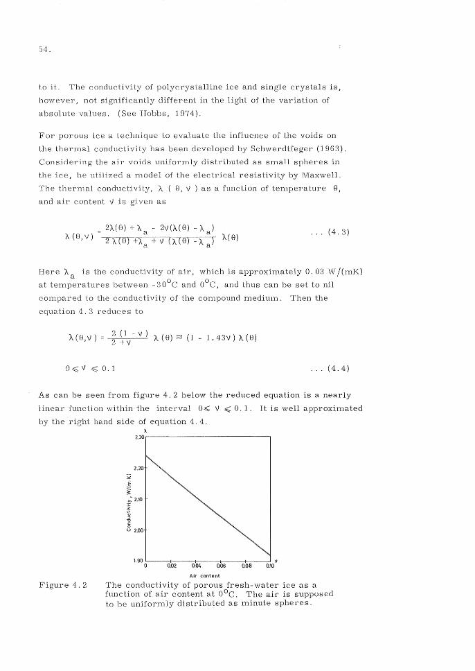
.54.
to it. The conductivity of polycrystalline ice and single crystals is J
hO\vever, not different in the light of the variation of
absolute values. (See Hobbs, 1974).
For porous ice a technique to evaluate the influence of the voids on
the thermal conductivity has been developed by Schwerdtfeger (1963).
the ice,
the air voids uniformly distributed as small spheres in
utilized a model of the electrical resistivity by Maxwell.
The 8, V ) as a function of temperature 8,
and air content v is as
(8, V) 2'A ( 8) + 'A a - 2V ('A ( 8) "A )
~:::-r;~;-;::----;--:--r.:--J~----:-__ a.....- 'A ( 8 ) ... (4.3)
Here 'A is the conductivity of air J which is approximately O. 03 Vii / (mK) a
at ternperatures between 300e and oOe, and thus can be set to nil
to the
equation 4. 3 reduces to
of the compound medium. Then the
A(8,v) A (8) ~ (1 1.43V) "A (8)
o ~ V ~ 0.1 ... (4.4)
As can be seen from figure 4. 2 below the reduced equation is a nearly
linear function within the interval O::S;: V .::;;;: O. 1. It is well approximated
the hand side of equation 4.4. A
1.90 0'----0::+:.0-2------:-10.0'::"":4--0+-.06--0-+.0-:8------'0.10 v
Air content
4.2 The conductivity of porous fresh-water ice as a function of air content at oOe. The air is supposed to be uniformly distributed as minute spheres.
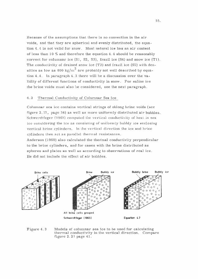
Because of the assumptions that there is no convection in the air
voids, and that they are spherical and evenly distributed, the equa
tion 4.4 is not valid for snow. Most natural ice has an air content
55.
of less than 10 % and therefore the equation 4.4 should be reasonably
correct for columnar ice (SI, S2, S3), frazil ice (S4) and snow ice (Tl).
The conductivity of drained snow ice (T2) and frazil ice (S5) with den
sities as low as 600 kg/m 3 are probably not well described by equa
tion 4.4. In paragraph 4.3 there will be a discussion over the va
lidity of different functions of conductivity in snow. For saline ice
the brine voids must also be considered, see the next paragraph.
4.2 Thermal of Columnar Sea Ice
Columnar sea ice contains vertical strings of oblong brine voids (see
figure 2. 17, page 34) as well as more uniformly distributed air bubbles.
Schwerdtfeger (1963) computed the vertical conductivity of heat in sea
ice considering the ice as consisting of uniformly bubbly ice enclosing
vertical bdne cylinders. In the vertical direction the ice and brine
cylinders then act as parallel therrnal resistances.
Anderson (1960) also calculated the ther'mal conductivity perpendicular
to the brine cylinders, and for cases with the brine distributed as
spheres and plates as well as according to observations of real ice.
He did not include the effect of air bubbles.
BrinE.' cells
Figure 4.3
Brine
All brine cells grouped
Schwerdtfe~r (1963)
Bubbly icE.' Bubbl y brine Bubbly icf'
Equation 4.7
Models of columnar sea ice to be used for calculating thermal conductivity in the vertical direction. Compare figure 2.21 page 41.
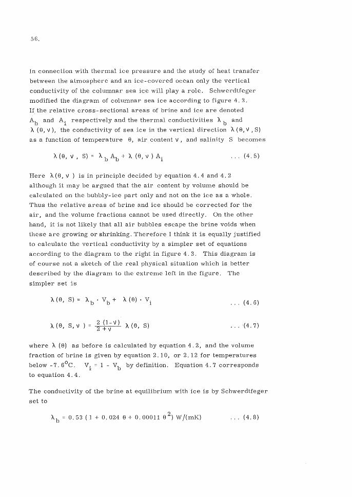
56.
In connection with thermal ice pressure and the study of heat transfer
between the atmosphere and an ice- covered ocean only the vertical
conductivity of the columnar sea ice will play a role. Schwerdtfeger
modified the diagram of columnar sea ice according to figure 4.3.
If the relative cross- sectional areas of brine and ice are denoted
Ab and Ai respectively and the thermal conductivities A band
A (8, V), the conductivity of sea ice in the vertical direction A (8, V , S)
as a function of temperature 8, air content V, and salinity S becomes
A (8 J V J S) = A b Ab + A (e J V ) Ai · .. (4.5)
Here A (8 J V ) is in principle decided by equation 4.4 and 4. 2
although it may be argued that the air content by volume should be
calculated on the bubbly- ice part only and not on the ice as a whole.
Thus the relative areas of brine and ice should be corrected for the
air J and the volume fractions cannot be used directly. On the other
hand, it is not likely that all air bubbles escape the brine voids when
these are growing or shrinking. Therefore I think it is equally justified
to calculate the vertical conductivity by a simpler set of equations
according to the diagram to the right in figure 4. 3. This diagram is
of course not a sketch of the real physical situation which is better
described by the diagram to the extreme left in the figure. The
simpler set is
A(8, S,V 2(1-V) A(8, S) 2 + V
· .. (4.6)
· .. '(4.7)
where A (8) as before is calculated by equation 4.2, and the volume
fraction of brine is given by equation 2.10, or 2.12 for temperatures
below -7. 6oC. V. = 1 - Vb by definition. Equation 4.7 corresponds 1
to equation 4.4.
The conductivity of the brine at equilibrium with ice is by Schwerdtfeger
set to
Ab = 0.53 (1 + 0.0248+ 0.00011 e 2)Wj(mK) · .. (4.8)
57.
The conductivity of the precipitated solid hydrates below -7. 6 0 C
is not well known, but it has a small influence on the bulk conductiv
ity' why it will be neglected here. For low temperatures when
V. 1
1 the bulk conductivity of columnar sea ice will asynlptotieal1y
tend to the value of fresh-water ice.
For temperatures close to the melting point, where the ice is more
than half liquid by volume, it is felt that the relations above give a
bad description of the heat flow. Probably convection will play a great
role, and may be the downward resistance to heat transfer will be
greater than the upward resistance.
Figure 4.4.
e -30 -20 -10 o
1"" .. nn""'''~:I!Tllr'''' J cC
2.75
2.50
2.25
2.00
1.75
1.50
The bulk conductivity of columnar sea ice as a function of temperature for different salinities Sand and air contents v according to the equations 4. 6 and 4. 7. The plotted values 0 are estimated by: Lewis (1966) from temperature profile data 0.7 0/00
< S < 4.5 0/00.
In figure 4.4 the hypothetical conductivity of sea ice according to
the equation 4.7 and 4. 6 above is drawn for some combinations
of air content and salinities. Values from an arctic- sea ice cover
calculated from measured temperature and salinity profiles by
58.
Lewis (1966) are also plotted in the figure for comparison. His
values roughly confirm the ideas in this paragraph.
4.3 Thermal of snow
The thermal conductivity of snow is much lower than that of ice,
because of the great contents of air. Therefore, a snow cover
effectively insulates an ice sheet from the temperature variations
in the air. Quite a few scientists have put up relations between snow
density and thermal conductivity. The results are rather scattered,
see below.
The scatter of conductivity coefficients might be due to the fact that
in snow the heat is only partly conducted. Other processes in dry
snow are radiant energy transfer between grains, mass transfer and
sublimation of water vapour along vapour-pressure gradients, and
mass transfer of air and vapour in convective flow. The radiant
energy transfer between grains is unimportant. Solar radiation must
be considered, however, see chapter 7. The convection could be
important for the upward flow of energy in loose snow in the ordi
nary case with cold air and "warm" ice, as this implies an unstable
density profile of the included air. In the warming-up case the
profile is however different, why the process does not matter.
In wet snow, on the other hand, the only important heat transfer pro
cess is the percolation of meltwater. All other processes give no
contribution as the gradients of temperature, vapour pressure and
air density are all nil. Solar radiation can still penetrate, of course.
In the discussion below it is assumed that the snow is considered
completely dry with neither vapour nor melt water in its pores. The
effect of the diffusion of water vapour and, especially, its condensa
tion and sublimation will be discussed in paragraph 6.3. The over
simplification may be responsible for some of the disparity between
the results on thermal conductivity of snow (Bader and Kuroiwa 1962).
Some results on snow conductivity was quoted by MelIor (1964),
table 4. 5, and an attempt to evaluate the proposed functions was
made by Anisimov (1961). The functions of table 4.5 are drawn in
figure 4.6.
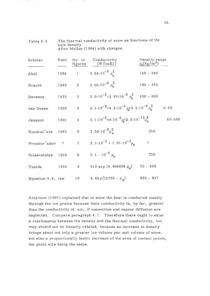
59.
Table 4.5 The thermal conductivity of snow as functions of its bulk density. After Mellor (1964) with changes.
Scholar Year No. in Conductivity Density range (W/(mK)) ps(kg/m 3 )
Abel 1984 2.84.10-6 p2 140 - 340 s
Bracht 1949 2 - 6 2
2. 05·10 Ps 190-350
Deveaux 1933 3 2. 9·1 0 - 2 + 2. 93.10 - 6 P; 100 - 600
van Dusen 1929 4 -2 -4 -9 3
2. 1·10 +4. 2·10 Pi2. 2·10 Ps > 50
Jansson 1901 5 -2 -4 -124
2. 1·10 +8·10 Pi2. 5·10 Ps
Kondrat' eva 1945 6 -6 2
3.56·10 Ps 350
Proskur'akov ? 7 2.1.10- 3 + -3 1.01·10 Ps ?
Sulakvelidze 1958 8 5. 1 . -4 lOPs 350
Yosida 1955 9 419 exp (0.004606 ps) 70 - 400
Equation 4.4, ice 10 4.48p/(2750 - ps) 825 - 917
Anisimov (1961) explained that in snow the heat is conducted mainly
through the ice grains because their conductivity is, by far, greater
than the conductivity of air, if convection and vapour diffusion are
neglected. Compare paragraph 4. 1. Therefore there ought to exist
a relationship between the density and the thermal conductivity, but
they should not be linearly related, because an increase in density
brings about not only a greater ice volume per unit volume of snow,
but also a proportionally faster increase of the area of contact points,
the grain size being the same.
80-500
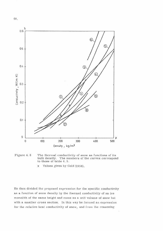
60.
A 0.6 ,....--------------------r----r-----t
0.5
0.4
:::L
E - 0.3 3:
.2':' > U ::J -u c
0.2 0 u
0.1
o L---------r---------r---------r---------+-------~ p o 100 200 300 400 500
Density J kg/m3
Figure 4.6 The thermal conductivity of snow as functions of its bulk density. The numbers of the curves correspond to those of table 4. 5.
x Values given by Gold (1958).
He then divided the proposed expression for the specific conductivity
as a function of snow density by the thermal conductivity of an ice
monolith of the same height and mass as a unit volume of snow but
with a smaller cross section. In this way he formed an expression
for the relative heat conductivity of snow, and from the reasoning

above this relative conductivity should increase with increasing
density, and formulas giving constant or even decreasing values
were dismissed. See figure 4.7. The functions disqualified are
numbers 4, 5, 7, 8 and 9
Figure 4.7
80
70
~ 60
~ ;§ 50 u ::l -0 C 40 0 u
ClI 30 .~
~ ClI
20 .a::::
10 P 100 200 300 400 500
Density, kg/m3
The "relative" conductivity of Anisimov (1961) in per cent. For an explanation see the text. The numbers of the curves are listed in table 4.5 and correspond to those in figure 4. 6.
Kondrat ~ eva'" s function, 6, on the other hand, that should be valid
when the density is greater than 350 kg/m3 , is disregarded because
it gives too high a specific conductivity. At 700 kg/m 3, for example,
it gives the same conductivity as that of pure ice, which obviously
must be wrong.
Equation 4.4, that is included in the list for reference only, gives
a "relative" conductivity of around 70 % within the range of snow
densities of interest. This is far better than what is reasonable for
snow, and, of course, that is because the snow structure and ice
structure is very different. The equation passes Anisimov'" s test
in the respect that the conductivity grows slightly faster than the
content of solid ice.
61.

62.
Of the remaining functions, numbers 1, 2 and 3, it is difficult to
prefer one to the other, because the conductivity of the snow is
likely to depend on the structure of the snow as well as on density.
The effect of grain size and shape have not been evaluated, to my
knowledge. In paragraph 3. 2 we concluded that reasonable bulk
density values of dry snow covers are 200 to 300 kg/m 3 . A con
servative value at 300 kg/m 3, giving an overestimation of the heat
flow through the snow cover, could be picked as 0.3 W /( mK) accord
ing to figure 4. 6.

63.
5. SPECIFIC AND LATENT HEATS
To estimate the heat exchange through an ice surface the condensation or
sublimation on the ice surface can be important. The heat capacity of a
piece of sea ice depends on the latent heat of melting of the ice in it and
the heat capacity of the contained brine and ice. Therefore some in
formation on the specific and latent heats of the substance of water is
given below. Most of the information is taken from Pounder (1965)
or Dorsey (1940).
5. 1 and Latent Heats of Water
The specific heat capacity of water is 4.23· 10 3 J /(kgK) at OOC, 3 0 3 0 .
4 . 27 . lOa t - 1 0 C, and 4. 35 . lOa t - 20 C.
To be able to calculate the heat capacity of a piece of sea ice, we
have to know the specific latent heat of fusion of water at different
temperatures. A rise of the temperature of sea ice involves, as
pointed out before, a gradual melting of ice. The specific latent
heat of fusion can be described by the following equation
L. = 3.34 . 105 (1 + 6.77 . 10- 3 8) J /kg 1
'" (5.1)
The latent heat of sublimation is mostly supposed to be the sum of the
latent heat of fusion and the latent heat of vapourization. Since the
latter two change in opposite directions with temperature the speci
fic heat of sublimation decreases but slowly from 2.84 . 106 J /kg
at _40 oC to 2.83 . 10 6 J/kg at OOC.
The determination of the specific heat capacity of fresh-water ice
presently considered most accurate was done by Dickinson and
Osborne in 1915, see for example Pounder (1965). For their measure
ments they used four very pure samples of ice between -40o C and
OOC. Their result could be fitted by equations of the form
2 C i = a + b 8 + c/8
where 8 is the temperature in °c and a, band c constants.
... (5.2)
a and b were the same for all specimens while c varied, c < O.

64.
The absolute value of c decreased with increasing purity of the
specimens, and c /L., where L. is the specific latent heat of 1 1
fusion of ice, was interpreted as the actual freezing point of the
solution. This will be shown to be true in paragraph 5.3 below.
The first two terms of equation 5. 1 would thus represent the true
specific heat of pure ice at constant pressure.
'" (5.3)
where
Co 2.12 103
J/(kg K)
and d
5.3 Heat of Sea Ice ------~----~----------
Essentially the heat capacity of a piece of sea ice depends on the
maSs of water changing state during the change of temperature, and
on the specific heat capacity of brine and pure ice. The heat capac
ity of dissolved salts is neglected. Denoting the specific heat capac
ities of pure water and ice by Cw
and C i respectively, the mass
ratios by mw and m i , and the specific latent heat of melting of
ice by Li' the following relation holds for the change of heat con
tent, dQ, at an increase in temperature d8, between -7. 60
C and
oOe.
dQ - L. dm. + C m dS + C. m. dS 1 1 W W 1 1
. ., (5.4)
The ratio of the mass of pure water to the whole mass is
... (5.5)
and introducing mb and m i from equations 2. 9a and b yields
dQ = _ L. S d s b + [~ ( C _ C.) + C. (1 _ S)] d S ... (5. 6) 1 ~ Sb w 1 1
From equation 2.5 sb = <11 Sand dSb = Cl 1 d8, and thus the
specific heat capacity of sea ice between the melting point Sm
and -7. 60 C is

65.
C(8S)=ddQ =_Li~+~(C -Ci)+(1-S)C
i ... (5.7)
, 8 a. e2 a. e w 1 1
Inspecting this equation it can be seen that for 8 ~ -] °c the first term
on the right hand side is two order of magnitudes greater than the second
term and that the first term corresponds to c /82 in equation 5. 2. Setting them equal gives
... (5.8)
which according to equation 2.5 is a good approximation of the
melting point em = s / a. 1 for low salinities.
Schwerdtfeger (1963) has shown that a calculation in the interval
_230
C ~ e < -7. 60
C within 2 % gives the same result as equation
5.7, in this way justifying its extension down to -23 0 C. Since it
C
~------------+-------______ ~ ____________ ~106
~
105 en ~----------~--~--------------r---------~~~ ~
Figure 5. ]
..........
u ~ 'u
~------------~------------~r---~----~--~104 ~ tf)
L-4--+--r--r~~4--+--r--r~--~-+--~~~103 8 -30 -20 -10 o
Temperature J QC
The specific heat capacity of sea ice as a function of salinity and temperature.
66.
approaches the specific heat of pure ice asymtotically for decreasing
temperatures, it can be used for practical purposes at even lower
temperatures. The specific heat capacity of the ice is drawn in
figure 5. 1 according to equation 5.7 for SOme salinities.
From the discussion above it is evident, that there is no true latent
heat of melting or melting temperature of sea ice, since the phase
change is continuous from sea ice to sea water. At the temperature,
e the heat deficit per unit mass (entalpity) relative to the melting
point Srn is by integration of equation 5.7.
Q= C(~, S)d~
... (5.9)
Assuming Li' Cw ' C i as constants the following relation appears
LiS 1 1 S Q =-- ( e -"8) + (1 - S) C i (e m - 8 ) + - (C - C. ) In e / e ( 5. 10)
CL1 m CL, w 1 m
The melting temperature is calculated by equation 2. 5. The result
of the integration is shown in figure 5. 2. As a comparison the curve
for pure ice with constant heat capacity is also plotted.
Strictly equation 5. 10 is valid only for e ;;. -7.6 °c but, in the light
of other uncertainties and that the deviation is only 2 % to the correct
value, it can be used for calculating the temperature change of a sea
ice cover down to -30 oC.
It should again be observed that equation 5.10 only holds for a closed
system of sea ice and brine .
daily temperature changes.
That is, the equation can be used for
For periods like months or years, gra-
vitational drainage and the movements of brine voids along tempera
ture gradients will change the salinity and thus the heat capacity of
the layers in an ice sheet. For fast temperature changes Ono (1966)
observed a temperature lag of O. 50 C for 20 minutes and O. 25°C
for 1 h in the voids of sea ice, so that the rate of change of tem-·

perature must not be too fast either. At temperatures close to the
melting point it is also doubtful whether equations 5.7 or 5. 10 give
a good description as the ice is fairly permeable to sea water.
Sometimes the concept latent heat is used about sea ice. It is then
meant the latent heat of the pure ice in an ice cover with a certain
salinity, S. If the salinity of the originally trapped brine was equal
to that of the ambient sea, Sa' it was shown in paragraph 2.53 that
the brine ratio at trapping was mb = S /S (equation 2. 13). Thus o a the corresponding ice ratio is m. (l-S/Sa) and consequently the
10
released latent heat is
67.
LS =( 1 - S/S ) L. a 1 .. . (5.] 1)
Figure 5.2
Q ~--------------------, 4.0 '105
3.0
1.0
~3~O-----------2~0-----------1~0---------~OO
Temperature.oC
The deficit of heat (negative entalpity) of sea ice relative to its freezing point as a function of temperature for the salinities 3 and 20 0/00, according to equation 5. 10 .
68.
The heat capacity of the ice phase of snow and porous ice is by
definition the product of its density and specific heat capacity.
This is, however, only true for snow or ice whose pores do not
contain melt water or vapour. In a similar way to what was done
with sea ice, the very correct heat capacity should be corrected
for the freezing, condensation or sublimation in the pores. For
snow, the migration or diffusion of water vapour should also be
taken into account. The melt water leaking down through a snow
cover may also cause a considerable redistribution of energy.
For snow an attempt to evaluate the influence of water vapour
is done in paragraph 6.3. Cold fresh-water ice could, however,
be considered completely dry. The small amount of water vapour
that is included has little influence on the thermal diffusion. In a
candIed ice cover, whose structure is very loose and filled with
water J the thermal diffusion will, of course, be greatly influenced.
6. TEMPERATURE DIFFUSIVITY
The diffusion equation 1. 1 is the basic tool for describing the rate
of change of temperature in a solid in terms of the boundary con
ditions. The properties of the solid appear in this equation in terms
of a single parameter, a, called the temperature diffusivity or the
coefficient of thermal diffusion. It is defined as
69.
a = ... (6.1)
where
A is the thermal conductivity
p is the density
C is the specific he!3-t capacity
The factor A is the quantity known with least accuracy. This is,
because it is difficult to evaluate it by the comparatively direct
way of equation 4.1, that is, by measuring a temperature gradient
and the corresponding heat flux, for the heat flux is extremely
difficult to measure. In fact most of the values in the literature on
the thermal conductivity of ice were obtained from studies on the
rate of change of temperature distributions, so that actually the
diffusivity was the constant measured. This was for example the
case with Lewis" s values on thermal conductivity in figure 4.4.
The quality of the values on thermal conductivity must, of course,
be judged with these problems in mind. For saline ice the difficulties
are still more pronounced, because the temperature diffusivity
is strongly dependent on the temperature and consequently the so
lution of the equation of diffusion is extremely difficult. It is felt
that, may be, the diffusivity of saline ice is better calculated in
directly from known properties of its constituents.
6.1 Temperature Diffusivity of Fresh-Water Ice
The coefficient of thermal diffusion of fresh-water ice can be cal
culated according to the functions for density, thermal conductivity
and capacity chosen in the earlier chapters. Experiments give
however the coefficient directly, see above.
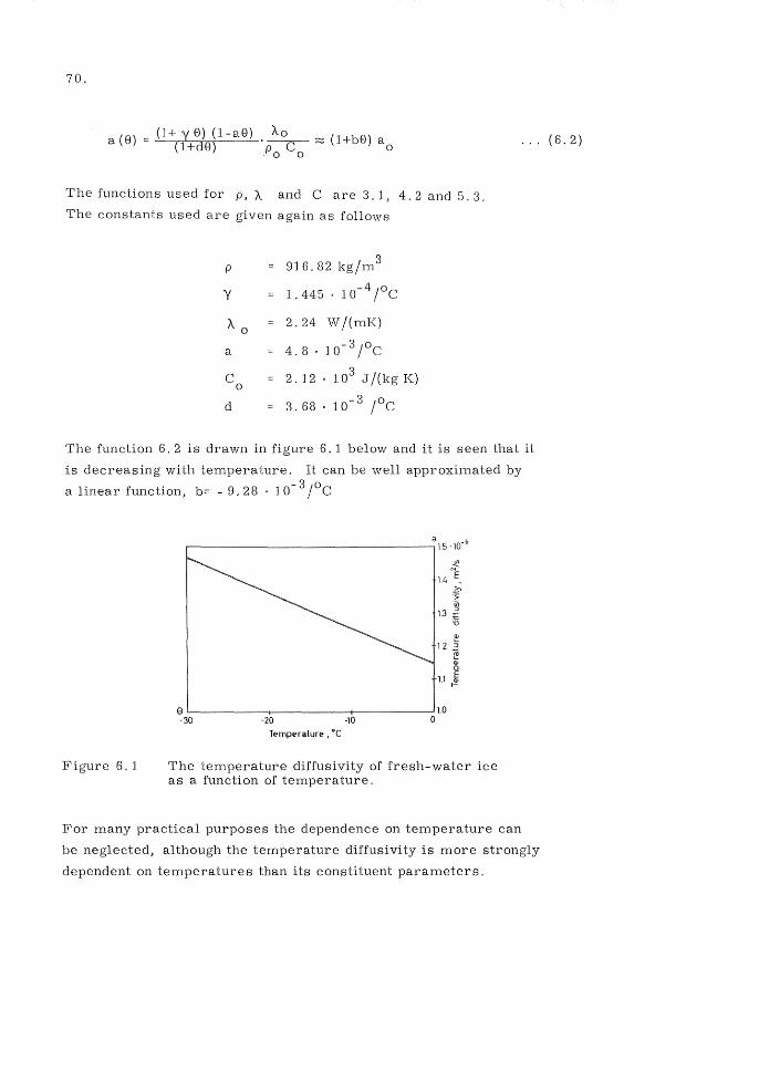
70.
a (8) (1+y8) (1-a8) AO
(1+d8)
The functions used for p, A and Care 3.1, 4.2 and 5.3.
The constants used are given again as follows
916.82 kglm 3 p
Y 1.445 . 1o-4/°e
A ° 2,24 W/(mK)
a 4,8 . lO-3/
oe
e 2, J 2 103
J/(kgK)
° d 3.68 10- 3 1°C
... (6.2)
The function 6. 2 is drawn in figure 6. 1 below and it is seen that it
is decreasing with temperature, It can be well approximated by
a linear function, b== - 9.28 . 10- 31oC
Figure 6.1
(IJ
12 :J . '@ (IJ 0-
1.1 ! 9 L..------i-------+--------' 1.0 -30 -20 -10 0
Temperature. GC
The temperature diffusivity of fresh-water ice as a function of temperature,
For many practical purposes the dependence on temperature can
be neglected, although the temperature diffusivity is more strongly
dependent on temperatures than its constituent parameters.
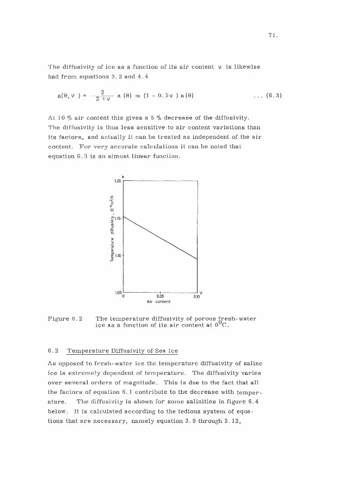
The diffusivity of ice as a function of its air content V is likewise
had from equations 3. 2 and 4.4
71.
a(8, V ) 2 a (8) ~ (1- O.5V) a(8) ... (6.3)
2 +V
At 10 % air content this gives a 5 % decrease of the diffusivity.
The diffusivity is thus less sensitive to air content variations than
its factors, and actually it can be treated as independent of the air
content. For very accurate calculations it can be noted that
equation 6.3 is an almost linear function.
Figure 6.2
a 1.20 r------------,
L05 '--------+-------' V o Q~ ruo
Air content
The temperature diffusivity of porous fresh-water ice as a function of its air content at oOe.
6. 2 Temperature Diffusivity of Sea Ice
As opposed to fresh-water ice the temperature diffusivity of saline
ice is extremely dependent of temperature. The diffusivity varies
over several orders of magnitude. This is due to the fact that .all
the factors of equation 6. 1 contribute to the decrease with temper
ature. The diffusivity is shown for some salinities in figure 6.4
below. It is calculated according to the tedious system of equa
tions that are necessary, namely equation 2.9 through 2.12,
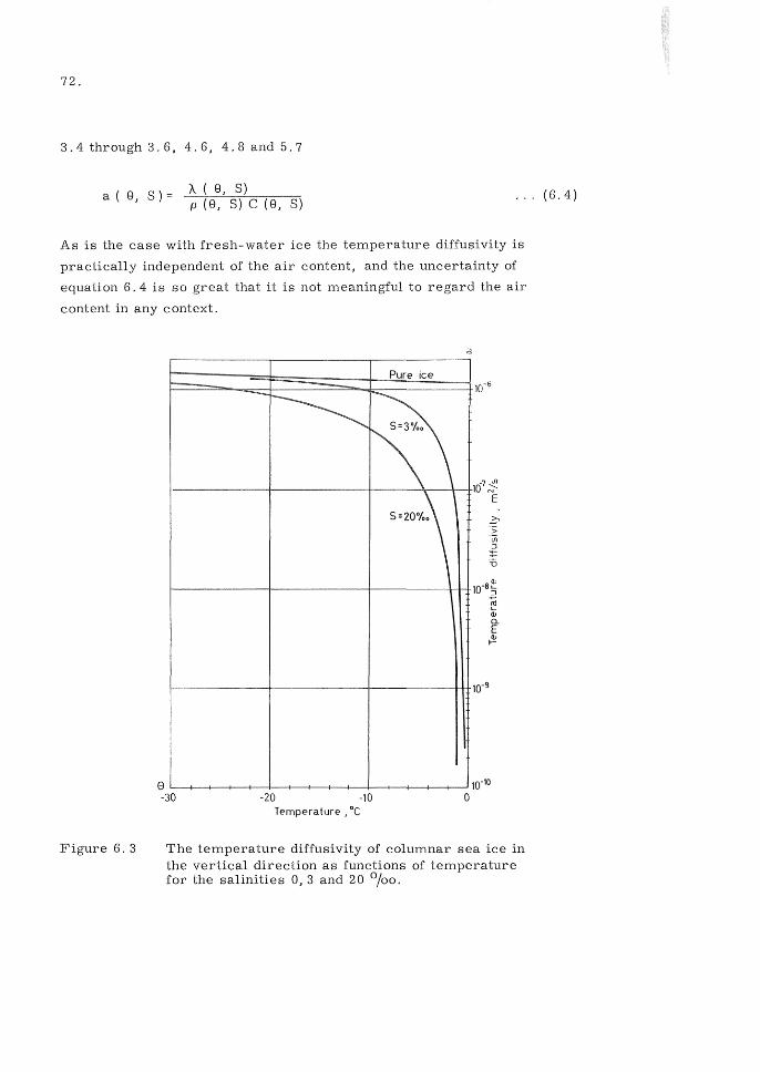
72.
3.4 through 3. 6, 4. 6, 4.8 and 5.7
a(9, S)= A ( 9, S) p (8, S) C (9, S)
... (6.4)
As is the case with fresh-water ice the temperature diffusivity is
practically independent of the air content, and the uncertainty of
equation 6.4 is so great that it is not meaningful to regard the air
content in any context.
Figure 6.3
i--
I
e -30
Pure ice ---~
K 5=20%0
-20 -10 Temperature 1°C
\
,
a
1
1 0-10
o
The temperature diffusivity of columnar sea ice in the vertical direction as functions of temperature for the salinities 0,3 and 20 0/00.
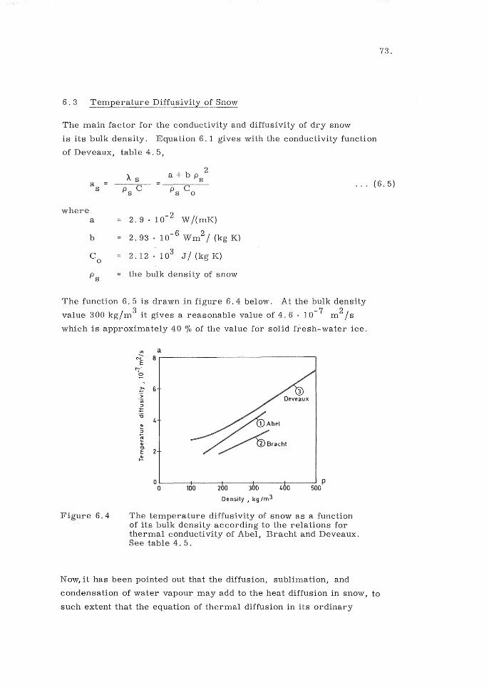
6.3 of Snow
The main factor for the conductivity and diffusivity of dry snow
is its bulk density. Equation 6. 1 gives with the conductivity function
of Deveaux, table 4.5,
2
73.
a + b Ps A s .. , (6.5) a
C s Ps Ps
where 10- 2 a 2.9 . W/(mK)
b 2.93 10- 6 Wm2 / (kg K)
C 2.12 103 J/ (kg K) 0
Ps the bulk density of snow
The function 6. 5 is drawn in figure 6.4 below. At the bulk density
value 300 kg/m 3 it gives a reasonable value of4.6. 10- 7 m 2 /s
which is approximately 40 % of the value for solid fresh-water ice.
Figure 6.4
~ a N 8
E 1';"'
0
:;;- 6 ";; "iij
~ :0
@.I
:5 Ai @; Cl. E 41 t-
O P 0 100 200 300 4 0 500
Density, kg 1m 3
The temperature diffusivity of snow as a function of its bulk density according to the relations for thermal conductivity of Abel, Bracht and Deveaux. See table 4. 5.
Now, it has been pointed out that the diffusion, sublimation, and
condensation of water vapour may add to the heat diffusion in snow, to
such extent that the equation of thermal diffusion in its ordinary
74.
form is no longer valid, and consequently values are not reliable
if they are founded on 6. 5 or on experiments presupposing equation
1.1.
as 1)[ ::: a ... (6.6)
Assume that the water vapour is saturated in the pores of the ice.
The mass of water vapour per unit volume, a w ' can then be con
sidered a function of only temperature.
In the equation of thermal diffusion the rate of sublimation of water
vapour per unit volume is included, that gives
as Of = a ... (6.7)
where
a is the bulk thermal diffusivity due to conduction
S temperature
time
x space coordinate
L the specific heat of sublimation
p the bulk density
C i the specific heat capacity of ice
q the mass rate of sublimation per unit volume
The equation of gas diffusion has a form equal to that of equation
6.7 and if the source of water vapour is included the following
relation appears
aa w
at
where aw is the mass content of water vapour per unit volume,
and D is the coefficient of gas diffusion in the porous medium
considered. D is of course a function of the structure of the snow.
In snow avalanches the vapour transport itself is of great import
ance, because the migration of the ice is responsible for the de
velopment of an avalanche structure of the snow.
(6.8)

75.
A combination of 6.7 and 6.8 gives
... (6.9)
This equation was formulated by Sulakvelidzw (1959). If we study
processes where a2 e / ax2 is of the same order of magnitude as
(ae /a x)2, the last term on the right hand side can be neglected.
A comparison with equation 6. 6 then gives the temperature
diffusivity as
a s a ... (6.10)
From equation 6.10 it can be seen that if a and D are of the same
order of magnitude the equation 6.6 is essentially correct. If
D < < a there will be a small reduction of the rate of change of
temperature due to local sublimation or condensation of water va
pour. On the other hand, if D > > a the temperature diffusivity
will be greater than the diffusivity due to conduction.
The molecular diffusion of equation 6. 10 can be set to the free
diffusion of air D = 3. 13 10- 4 m 2 / s and the thermal diffusion can -6 2/ be set to that of the ice phase a = 1. 15 10 m s. Both constants
are overestimations because the molecular diffusion is restricted
by the snow flakes and the conduction is restricted by the bad contact
between grains. Inserted in 6. 10 they give the quotient a/a to ° 0 3 s 0 1.45 at 0 e and 1.10 at -20 e for p = 300 kg/m. At -30 e the
difference between a and as can be neglected. For very loose
snow the quotient a /a grows to over 2 at oOe. (p = 150 kg/m 3, s e = oOe a la = 1. 9). It is thus obvious that the heat transport s by mass diffusion along the gradient of vapour pressure should not
be disregarded.
76,
As the temperature of the snow is not given in context with rec
ommended formulas on heat conduction, the mass diffusion is
one reason to blame the discrepances between the formulas as
well as the structure of the snow. It would be interesting to
evaluate the formulas by means of equation 6,10. In lack of
this evaluation the function of Deveaux will be used.
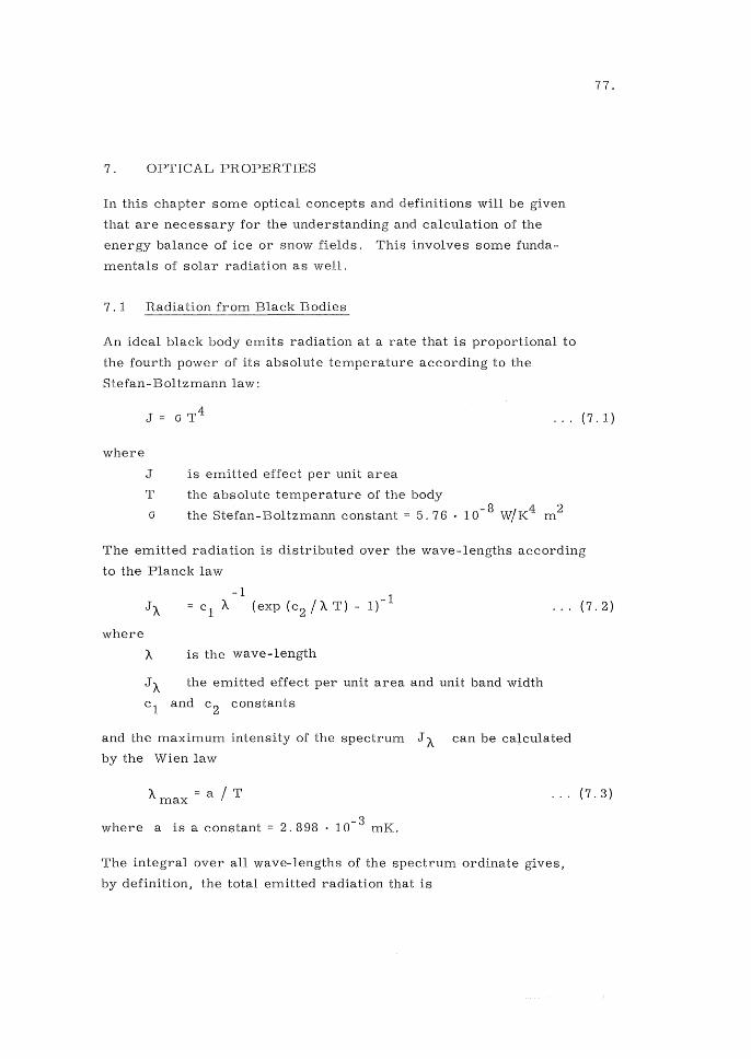
7. OPTICAL PROPERTIES
In this chapter some optical concepts and definitions will be given
that are necessary for the understanding and calculation of the
energy balance of ice or snow fields. This involves some funda
mentals of solar radiation as well.
7. 1 Radiation from Black Bodies
An ideal black body emits radiation at a rate that is proportional to
the fourth power of its absolute temperature according to the
Stefan-Boltzmann law:
77.
... (7.1)
where
J is emitted effect per unit area
T the absolute temperature of the body
G the Stefan-Boltzmann constant = 5.76 .10- 8 w/K4 m 2
The emitted radiation is distributed over the wave-lengths according
to the Planck law
-1 = cl A (exp (c2 lA T) - 1)-1 ... (7.2)
where
A is the wave-length
J A the emitted effect per unit area and unit band width
cl and c 2 constants
and the maximum intensity of the spectrum J A can be calculated
by the Wien law
A max a I T ... (7. 3)
where a is a constant 2.898· 10- 3 mK.
The integral over all wave-lengths of the spectrum ordinate gives,
by definition, the total emitted radiation that is
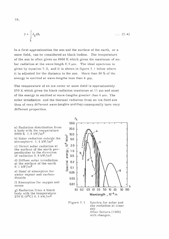
78.
. .. (7.4)
In a first approximation the sun and the surface of the earth, or a
snow field, can be considered as black bodies. The temperature
of the sun is often given as 6000 K which gives the maximum of so
lar radiation at the wave-length 0.5 }lm. The ideal spectrum is
given by equation 7.2, and it is shown in figure 7.1 below where
it is adjusted for the distance to the sun. More than 99 % of the
energy is emitted at wave-lengths less than 4 }lm.
The temperature of an ice cover or snow field is approximately
270 K which gives its black radiation maximum at 11 }lm and most
of the energy is emitted at wave-lengths greater than 4 }lm. The
solar irradiation and the thermal radiation from an ice field are
thus of very different wave-lenghts and they consequently have very
different properties.
a) Radiation distribution from a body with the temperature 6000 K 1. 6 k'vV 1m2
b) Solar radiation outside the atmosphere 1.4 kW 1m2
c) Direct solar radiation at the surface of the earth perpendicular to the direction of radiation O. 9 kW I m2
d) Diffuse solar irradiation at the surface of the earth 0.lkW/m2
e) Band of absorption for water vapour and carbondioxide
f) Absorption for oxygen and ozone
g) Radiation from a black body with the temperature 270 K (OOe) 0.3 kW 1m2
JA,
50.0
20.0
10.0
5.0
2.0
:>. 1.0 CTI b Qj c 0.5 Q)
~ 0.2 ..... u
0.1 Q) a. (/) 0.05
0.02
0.01
0.1 0.2 0.5 10 2.0 5.0 10 20
Wav@length J 10- 6 m
A, 50 100
Figure 7.1 Spectra for solar and sky radiation at clear sky. After Sellers (1965) with changes.

7. 11 Solar Radiation
At the outer boundary of the atmosphere the distribution of solar
radiation is very accurately given by equation 7. 2 for the visible
and infrared part of the spectrum (A > 0.4 pm). See figure 7. 1.
The radiation flux is approximately 1.4 kW 1m2, and although this
figure depends on the distance to the sun,"±' 3.4 0/0, it is some
times referred to as the solar constant.
When the solar radiation enters and penetrates the atmosphere of
the earth it is effected in several ways by the gases, clouds and
particles in the atmosphere. It is out of scope of this book to give
detailed information on this matter. A few facts will, however, be
given. For further details it is referred to standard literature like
the textbooks by Sellers (1965), Liljequist (1962) or Brunt (1944).
Radiation of wave lengths shorter than 0.2 }lm is completely absorbed
by ozone and oxygen, and therefore this radiation never reaches the
surface of the earth. Furthermore water-vapour and carbon dioxide
absorb radiation within several wave-length bands. The abserbed
radiation is of course transformed into heat.
79.
The direct solar radiation is also reduced by scattering. The scattering
caused by the molecules of the air is most intensive for short wave
lengths, and this makes the sky blue. Bigger particles as water drops,
ice crystals and dust, on the other hand, scatter light equally over the
spectrum. Hazy or dusty air therefore gives the sky a whitish com
plexion, and the clouds look white. When the altitude of the sun is
lowered, the rays of the sun have to pass a longer way through the
atmosphere, and a greater part of the short waves is scattered causing
the sun to appear red.
The irradiation at the ground level is composed of direct solar radi
ation and scattered so called sky radiation. On a clear day the direct
radiation is approximately 0.9 kW 1m2 and the sky radiation 0.1 kW 1m2 .
On an overcast day the global irradiation is largely diffuse and only
a fourth of that of a clear day.
The spectral distribution of the irradiation depends on the shifting
atmospheric conditions particularly the water vapour content and
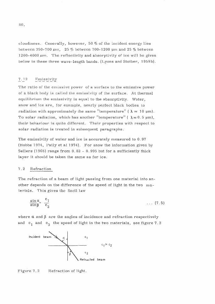
80.
cloudiness. Generally, however, 50 % of the incident energy lies
between 350-700 .um, 25 % between 700-1200 pm and 25 % between
1200-4000,um. The reflectivity and absorptivity of ice will be given
below in these three wave-length bands. (Lyons and Stoiber, 1959b).
7.12
The ratio of the emissive power of a surface to the emissive power
of a black body is called the emissivity of the surface. At thermal
equilibrium the emissivity is equal to the absorptivity. Water,
snow and ice are, for example, nearly perfect black bodies to
radiation with approximately the same "temperature" ( A ~ 10 pm).
To solar radiation, which has another "temperature" ( A -;::::. O. 5 pm),
their behaviour is quite different. Their properties with respect to
solar radiation is treated in subsequent paragraphs.
The emissivity of water and ice is accurately measured to O. 97
(Bobbs 1974, Paily et al 1974). For snow the information given by
Sellers (1965) range from 0.82 - 0.995 but for a sufficiently thick
layer it should be taken the same as for ice.
7. 2 Refraction
The refraction of a beam of light passing from one material into an
other depends on the difference of the speed of light in the two ma
terials. This gives the Snell law
sin sin~
... (7.5)
where a. and ~ are the angles of incidence and refraction respectively
and cl and c 2 the speed of light in the two materials, see figure 7.2
Incident beam
Refracted beam
Figure 7.2 Refraction of light.
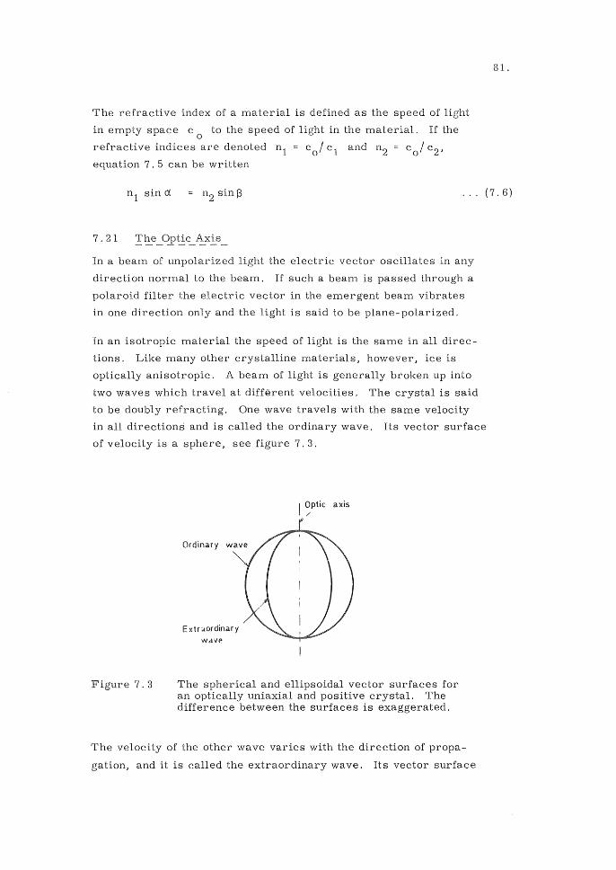
The refractive index of a material is defined as the speed of light
in empty space c 0 to the speed of light in the material. If the
refractive indices are denoted n1 = col cl and n 2 = col c 2 '
equation 7. 5 can be written
81.
... (7.6)
7.21
In a beam of unpolarized light the electric vector oscillates in any
direction normal to the beam. If such a beam is passed through a
polaroid filter the electric vector in the emergent beam vibrates
in one direction only and the light is said to be plane- polarized.
In an isotropic material the speed of light is the same in all direc
tions. Like many other crystalline materials, however, ice is
optically anisotropic. A beam of light is generally broken up into
two waves which travel at different velocities. The crystal is said
to be doubly refracting. One wave travels with the same velocity
in all directions and is called the ordinary wave. Its vector surface
of velocity is a sphere, see figure 7.3.
Figure 7.3
Ordinary wave
E xtr;.tordinar y WdVP.
I ~ptic axis
The spherical and ellipsoidal vector surfaces for an optically uniaxial and positive crystal. The difference between the surfaces is exaggerated.
The velocity of the other wave varies with the direction of propa
gation, and it is called the extraordinary wave. Its vector surface
82.
wave is an ellipsoid of revolution, and in the case of optically uni
axial crystals, like ice, the spherical vector surface coincides with
the ellipsoidal surface at two points only, and these are the ends of
the axis of revolution of the ellipsoid. If the extraordinary wave is
slow relative to the ordinary wave the crystal is said to be optically
positive, otherwise optically negative.
The electric vector of the ordinary wave always oscillates perpen
dicular to the optic axis, that is, perpendicular to a plane defined
by the direction of propagation and the axis. The electric vector of
the extraordinary wave oscillates in the plane. The ordinary wave and
ext rao rdinary wa ve a re thus polarized at right angles to each other.
Ice is a doubly refracting, uniaxial, and optically positive crystal.
The optic axis coincides with the crystallographic c-axis.
7. 22 Refractive Indices
Two principal indices are defined for uniaxial crystals, one based
on the velocity of the ordinary wave c the other on the velocity of
the extraordinary wave perpendicular to the c- axis. For ice this is
the minimum velocity c e ' Thus
... (7.7)
The quantity ne - no is called the birefringence of the crystal.
Measurements of ne and no are accounted for by Hobbs (1974).
They vary both with wave-length and temperature. Here, we shall
only notice that ice has the lowest refractive indices of all the known
minerals. At _3 0 C and 0.4916)lm n 1. 3126 and n = 1.3140. o e
The birefringence is thus also small: 0.0014.
7.23 Polarization Effects
Plane- polarized light that is transmitted through an ice crystal at
some angle of incidence to the optic axis will generally not be polar
ized in the original plane when leaving the crystal, due to the re-
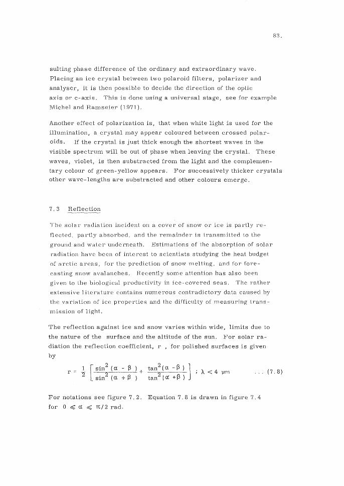
suIting phase difference of the ordinary and extraordinary wave.
Placing an ice crystal between two polaroid filters, polarizer and
analyser, it is then possible to decide the direction of the optic
83.
axis or c-axis. This is done using a universal stage, see for example
Michel and Ramseier (1971).
Another effect of polarization is, that when white light is used for the
illumination, a crystal may appear coloured between crossed polar
oids. If the crystal is just thick enough the shortest waves in the
visible spectrum will be out of phase when leaving the crystal. These
waves, violet, is then substracted from the light and the complemen
tary colour of green-yellow appears. For successively thicker crystals
other wave-lengths are substracted and other colours emerge.
7 . 3 Reflection
The solar radiation incident on a cover of snow or ice is partly re
ilected. partly absorbed, and the remainder is transmitted to the
ground and water underneath. Estimations of the absorption of solar
radiation have been of interest to scientists studying the heat budget
of arctic areas, for the prediction of snow melting, and for fore
casting snow ava] anches. Recently Born e attention has also been
given to the biological productivity in ice-covered seas. The rather
extensive literature contains numerous contradictory data caused by
the variation of ice properties and the difficulty of measuring trans
m ission of light.
The reflection against ice and snow varies within wide, limits due to
the nature of the surface and the altitude of the sun. For solar ra
diation the reflection coefficient, r , for polished surfaces is given
by
l' = A <4 '!lm ... (7.8)
For notations see figure 7. 2. Equation 7.8 is drawn in figure 7.4
for 0 ~ Cf. ~ TC/2 rad,
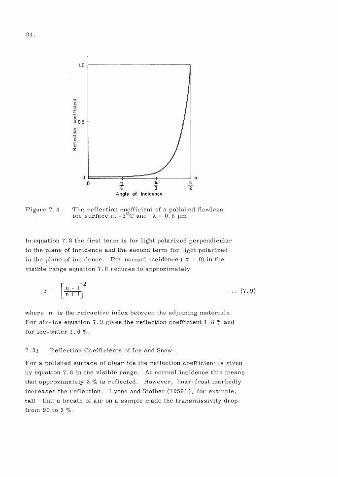
84.
Figure 7.4
c CiI
~ ..... CiI
1.0 ...-----------------"
30.5
o I:::::=~~~~~==__+_----.J o 'It 'It
6" "3 'It
'2 Angh~ of incidence
The reflection coefficient of a polished flawless ice surface at - 30 C and f... = 0.5 pm.
In equation 7.8 the first term is for light polarized perpendicular
to the plane of incidence and the second term for light polarized
in the plane of incidence. For normal incidence (a. 0) in the
visible range equation 7. 8 reduces to approximately
r = [d2
n + 1J ... (7. 9)
where n is the refractive index between the adjoining materials.
For air-ice equation 7.9 gives the reflection coefficient 1.8 % and
for ice-water 1. 6 0/0.
7. 31 Reflection Coefficients of Ice and Snow
For a polished surface of clear ice the reflection coefficient is given
by equation 7. 8 in the visible range. At normal incidence this means
that approximately 2 % is reflected. However I hoar-frost markedly
increases the reflection. Lyons and Stoiber (1959 b), for example,
tell that a breath of air on a sample made the transmissivity drop
from 90 to 3 0/0.
Light may also be reflected from particles, bubbles or brine voids
enclosed in the ice and not only from the very surface. Thomas
(1964) measured reflection coefficients of 65 and 66 % at solar alti
tudes of 24 0 09 " and 90 27" respectively for sea ice under natural
conditions. For the corresponding angles of incidence figure 7.4
gives 9 and 68 %. In both cases the reflection must have been large
] y diffuse. Gaitskhoki (197 Oa) m easured coefficients of ref] ection
for normal incidence on sea ice in the laboratory in the wave-length
band 0.35 Jlm -1. 0 1JIYl. are for different types of ice in
figure 7.8. For ice, bubbly ice, snow ice, and sea ice the results
range from 4% to 15%. For snow he got 65 to 80 %.
Mellor (1965) measured reflection against natural snow fields. His
results showed a reflection coefficient ranging between 77 and 98 %, see figure 7.5. By comparing extinction data, paragraph 7.4, with
the measured surface reflection he could show that only 40-80 % of
the reflected energy was reflected from the very surface of the snow
field. The remainder must therefore be reflected from grains at
some depth in the snow. Bergen (1975) tried to relate the albedo
to the grain size and density of the snow cover. The deducted ex-
pression looks promising, but the only available test values were
reflection coefficients between 85 and 78 %. See also Bader and
Kuroiwa (1962).
The crystal orientation in an ice cover is observed to influence the
reflection coefficient of ice. Lyons and Stoiber (1963) state that
microscopic vapour bubbles form within the ice crystals when an
ice cover is warmed. The phenomenon is called Tyndall 'figures.
The vapour leaves the crystal along the basal planes, and therefore
ice with vertical basal planes (horizontal c-axes, ice S2) soon get
rid of the vapour bubbles, but if the basal planes are horizontal
(vertical c-axes, ice SI) the figures stay in the ice. The latter
ice gets a grayish appearance and reflects light better. Because
of this the crystal orientation of an ice field can some times be
seen with the bare eye in spring, when the ice cover has been ex
posed to the sun. The vertically oriented crystals are grayish and
a little elevated above the surrounding crystals.
85.
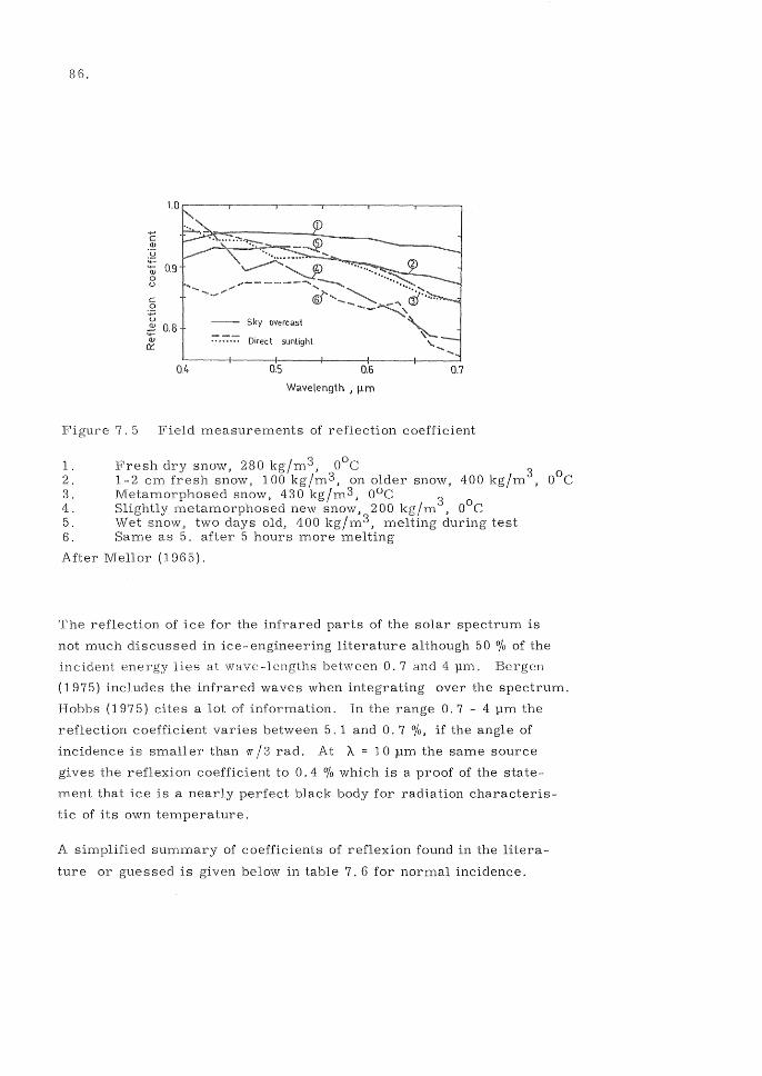
86,
C .~
~ QJ
0 U
C 0
:.;:; u
~ QJ
a::
1.0
0.9
0.8
0.4
Sky overcast
Direct sunlight
0.5 0.6
W;avelength J IJ.m
0.7
Figure 7. 5 Field measurements of reflection coefficient
1. Fresh dry snow, 280kg/m3, oOe 3 2. 1 2 cm fresh snow J 100 kg/m 3, on older snow, 400 kg/m , oOe 3. Metamorphosed snow, 430 kg/m 3, oOe 3 4. Slightly metamorphosed new snow, 200 kg/m , oOe 5. Wet snow, two days old, 400 kg/m3, melting during test 6. Same as 5. after 5 hours more melting
After Mellor (1965).
The reflection of ice for the infrared parts of the solar spectrum is
not much discussed in ice- engineering literature although 50 % of the
incident energy lies at wave -lengths between 0,7 and 4 pm. Bergcn
(1975) includes the infrared waves when integrating over the spectrum.
Bobbs (1975) cites a lot of information. In the range 0.7 - 4 pm the
reflection coefficient varies between 5. 1 and O. 7 %, if the angle of
incidence is smaller than 'ff /3 rad. At A 10 pm the same source
gives the reflexion coefficient to 0.4 % which is a proof of the state
ment that ice is a nearly perfect black body for radiation characteris
tic of its own temperature.
A simplified summary of coefficients of reflexion found in the litera
ture or guessed is given below in table 7. 6 for normal incidence.
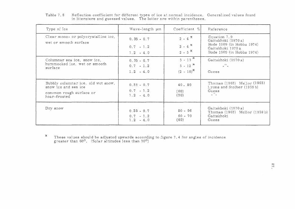
Table 7.6 Reflection coefficient for different types of ice at normal incidence. Generalized val ues found in literature and guessed values. The latter are within parentheses.
Type of Ice \Vave-length :um Coefficient 0/0 Reference
Clear mono- or polycrystalline ice, O. 35 - O. 7 2 _ 4 x Equation 7. 9
wet or smooth surface Gaitskhoki (1970 a)
0.7 - 1. 2 2 _ 4 li Bode 1909 (in Hobbs 1974) Gaitskhoki 1970 a
1.2 - 4.0 2 - 5 li Bode 1909 (in Hobbs 1
Columnar sea ice, snow ice, O. 35 - O. 7 5 - 15~ Gaitskhoki (1970 a) hummocked ice. wet or smooth 0.7 - 1. 2 .5 - 12 * - !! -surface
1.2 - 4.0 (2 - 10)* Guess
Bubbly columnar ice, old wet snow, 0.35 - 0.7 40 _ 80 Thomas (1963) Mellor (1965) snow ice and sea ice Lyons and Stoiber (1959 b)
common rough surface or 0.7 - ]. 2 (60) Guess
!!
hoar-frosted 1.2 - 4.0 (30) - -
Dry snow 0.35 - 0.7 80 - 96
Gaitskhoki (1970 a) Thomas (1963) Mellor (1959 b)
0.7 - 1. 2 60 - 70 Gaitskhoki 1.2 - 4.0 ( 60) Guess
:if These values should be adjusted upwards according to figure 7.4 for angles of incidence greater than 60 0 . (Solar altitudes less than 30°)
(Xl
-J
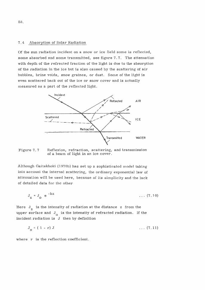
88.
7.4 of Solar Radiation
Of the sun radiation incident on a snow or ice field some is reflected,
some absorbed and some transmitted, see figure 7. 7. The attenuation
with depth of the refracted fraction of the light is due to the absorption
of the radiation in the ice but is also caused by the scattering of air
bubbles, brine voids, snow graines, or dust. Some of the light is
even scattered back out of the ice or snow cover and is actually
measured as a part of the reflected light.
// Reflected AIR
11 /
/ "*
Scattered _-L' _____ ~_--_ ICE
WATER
Figure 7.7 Reflexion, refraction, scattering, and transmission of a beam of light in an ice cover.
Although Gaitskhoki (1970b) has set up a sophisticated model taking
into account the internal scattering, the ordinary exponential law of
attenuation will be used here, because of its simplicity and the lack
of detailed data for the other
J z J o e -kz ... (7.10)
Here J z is the intensity of radiation at the distance z from the
upper surface and J 0 is the intensity of refracted radiation. If the
incident radiation is J then by definition
J = ( 1 - r) J o
where r is the reflection coefficient.
... (7.11)

89.
For flawless fresh-water ice k equals the absorption coefficient.
For natural ice, snow, or turbid water, where the equation is only
approximately valid, k is often called the coefficient of extinction.
In such cases it takes into account both absorption and scattering.
It should be pointed out that in optics another quantity is meant by
the extinction coefficient J1 which is the imaginary part of the
complex refractive index and related to k (for flawless ice) by
k=47fp/'A
where A is the wave-length.
100
90
80
.,..e 70 I)
.2 60 ...-~ L-
e 50 .2 U) U)
'E 40 U)
e ~ .= 30
10 ~~4----+--~----+---4----+--~
o 0.3 0.4 0.5 0.6 0.7 0.8 0.9 1.0
Wave - length J IJ.m
... (7.12)
monolithic ice p = 917 kg/m3
without any air inclusion, reflexion coefficient r = O. 04
ordinary ice p = 895 kg/m3 0.05~r~0.06
columnar sea ice p 915kg/m 3
0.11~r~0.14
snow ice p = 877 kg/m 3
0.10~r~0.12
surface layer of sea pack ice 0.10~r~0.15
snowp = 280 kg/m 3
A
(0.35 J1m~A~ 0.8 mm r = 0.80
{A S'::j 1. 0 pm r = 0.65
Figure 7.8. Spectral curves of the ratio of transmitted light for sample of ice 2 cm thick. Gaitskhoki (1970 a).

90.
7. 41 ~E~o~E!i~!y_0J~~
Lyons and Stoiber (1959b) have written a critical review of older investigations
on the absorptivity of ice and have also performed a lot of measurements
themselves. They measured the transmission through samples and cor
rected for reflection at the upper and lower surfaces using equation (7.9).
Another method is to embed photocells at different depths in an ice cover,
that is, to measure Jz at several different depths. This latter method
was used by Thomas (1964). Gaitskhoki (1970 a) used samples but meas-
ured both reflected and transmitted light. Older investigations cited
by Lyons and Stoiber (1959 b) were made with samples of different thick
nesses. This method is, however, less accurate according to them.
In order to show how greatly the absorption can differ, the transmission
ratio through 2 cm thick samples of ice and snow as measured by Gaitskhoki
(1970 a) is given in figure 7.8.
The order of magnitude of the extinction coefficient in the visible region
is 1 m- 1, but passing into the infrared region the absorptivity of ice
increases sharply. For example a plate of ice 1 mm thick absorbs prac
tically all radiation for which the wavelength is greater than 3 \-Lm and a
frozen soap-film cuts off nearly all radiation with wave-lengths greater
than 6 \-Lm. A part of the infrared absorption spectrum is given in figure
7.9 below. The absorption for long wavelengths (A> 1.2 !lm) is less de
pendent on the air content and purity of the ice, because the absorption
is due to molecular and intermolecular vibrations in the lattice. For
further details see Hobbs (1974).
..... C G1
:~ --~ u
k 107~~--~--~--~--~--~--.--.
106
105
104
2 3 4
..!\-Lm
A 5
Figure 7. 9 Infrared absorption spectrum of ice in the range 1. 4 I-Lm~ A ~ 4 \-Lm. After Bobbs (1974) with changes.
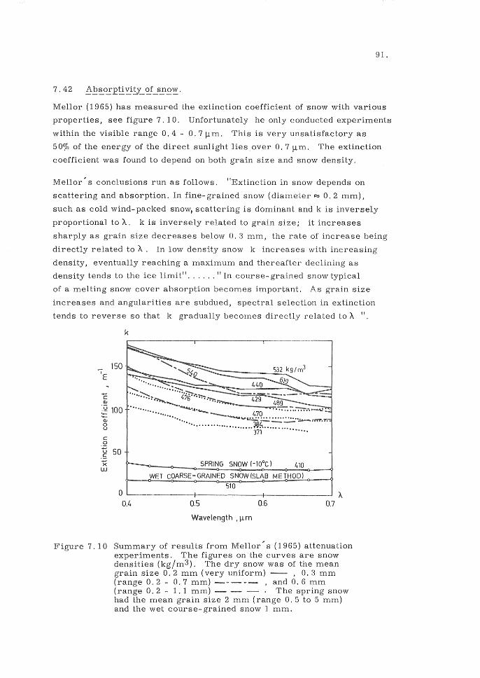
91.
7. 42 ~E~o.!E!J:~!y_~_s.E~~'
Mellor (1965) has measured the extinction coefficient of snow with various
properties, see figure 7. 10. Unfortunately he only conducted experiments
within the visible range 0.4 - O. 7 /l m. This is very unsatisfactory as
50% of the energy of the direct sunlight lies over 0.7 j..Lm. The extinction
coefficient was found to depend on both grain size and snow density.
Mellor" s conclusions run as follows. "Extinction in snow depends on
scattering and absorption. In fine- grained snow (diameter ~ 0.2 mm),
such as cold wind- packed snow, scattering is dominant and k is inversely
proportional to A.. k is inversely related to grain size; it increases
sharply as grain size decreases below O. 3 mm, the rate of increase being
directly related to A.. In low density snow k increases with increasing
density, eventually reaching a maximum and thereafter declining as
density tends to the ice limit 11 •••••• " In course- grained snow typical
of a melting snow cover absorption becomes important. As grain size
increases and angularities are subdued, spectral selection in extinction
tends to reverse so that k gradually becomes directly related to A. 11
_ 150 lE
C <!J
k
~ 100 a:; o u
c .9 U .S x w
50
o 0.4
SPRING SNOW (-lOOe) 410
WET COARSE-GRAINED SNOW(SLAB METHOD)
510
os 0.6
Wavelength,ll m
A. 0.7
Figure 7. 10 Summary of results from Mellor" s (1965) attenuation experiments. The figures on the curves are snow densities (kg/m3 ). The dry snow was of the mean grain size 0.2 mm (very uniform) , 0.3 mm (range 0.2 - 0.7 mm) -- --, and 0.6 mm (range 0.2 - 1.1 mm) - The spring snow had the mean grain size 2 mm (range 0.5 to 5 mm) and the wet course- grained snow] mm.
92.
7.43 Generalized Values on the Extinction Coefficient.
Table 7.11 below is a summing-up of available information on the ex
tinction coefficient. The values for clear ice and bubbly ice are those
recommended by Lyons and Stoiber (1959 b). The basis for the other
figures are given in the table. The given values are supposed to be accu
rate within one order of magnitude if taken as mean values over respective
range of wave-length. For reference some values for water are also listed.

Table 7.11. Coefficient of extinction for different types of ice. Generalized values found in literature and guessed values. The latter are within parentheses.
l Type of ice Wave-length \-Lm Coefficient m -1 Reference
Clear fresh-water 0.35-0.7 0.2 Lyons and Stoiber (1959 b) ice 0.7 - 1. 2 2 " SI, S2 1. 2 . - 4 (5000)
II
I ~ubbly fresh-water 0.35 - 0.7 3 Lyons and Stoiber (1959 b) i Ice 0.7 - 1. 2 (10) "
SI, S2 1.2 - 4 (10000) "
Columnar sea ice 0.35 - 0.7 2 Thomas (1964)
0.7 - 1. 2 10 Gaitskhoki (1970)
1.2 - 4 (l0000) Guess
"Bubbly r sea ice 0.35 - 0.7 40 Gaitshoki (1970)
Surface layer dried 0.7 - 1. 2 70 " of salt
1.2 - 4 (10000) Guess
Snow ice 0.35 - 0.7 30 Gaitskhoki (1970)
0.7 - 1. 2 50 " 1.2 - 4 (10000) Guess
Fine-grained snow 0.35 - 0.7 120 Mellor (1965) mean diameter 0.7 - 1. 2 200 Gaitskhoki (1970) 0.2 - 0.6 mm
1.2 - 4 (10000) Guess
Course- grained 0.35 - 0.7 30 Mellor (J 965) snow, mean dia- 0.7 - 1. 2 (200) Guess meter 1-2 mm
1.2 - 4 (10000) Guess
Pure water 0.35 - 0.7 0.05 Harvey (1966)
Ocean water 0.35 - 0.7 0.20 " Coastal water 0.35 - 0.7 0.45 !!
co CA?
94.
8. ENERGY BALANCE OF AN ICE OR SNOW COVER
The energy balance of ice or snow covers have mostly been studied in
order to evaluate their growth or decay. Although such studies have
often been performed with sophisticated methods, they work with daily,
weekly, or monthly mean values, why they can seldom be used directly
for the calculation of the fast temperature fluctuations that are respon
sible for thermal ice pressure.
On the other hand, studies aiming at thermal ice pressures tend to
oversimplify the energy balance of the surface by simply setting the
surface temperature equal to the air temperature, or only calculating ad
vective heat transfer. The short and long wave radiation play, however,
very important roles. The short wave radiation increases the rate of
change of temperature, especially, at clear weather. The long wave
back radiation can cause a considerable depletion of the ice surface
temperature, which is very pronounced by clear and calm weather.
Omitting radiation therefore results in an underestimation of the daily
temperature variations in an ice cover.
Below follows some fundamentals of the heat balance just in order to
place the thermal and optical properties of ice and snow in a wider con
text. For evaluations of heat balance functions it is referred to Paily
et al (1974) or Sweers (1976) and for a discussion of the balance of ice
or snow fields to Pounder (1965), Liljequist (1962), or Bengtsson (1976).
The energy flux of an ice cover can be written
..... (8.1)
where
qt is the rate of change of stored heat per unit area due to change of temperature of the ice or snow
qe the rate of heat per unit area used for evaporation
qm the rate of heat used to melting per unit area
qc convective (sensible) heat flux
qb intensity of long-wave back radiation
ql intensity of incoming long-wave radiation
qs net incoming short-wave radiation flux
95.
The only term of equation (8.1) above that has not been accounted for
at all in this text is the convective heat transfer qc which is a complicated
function of wind speed, the stability of the air near the ground, and the
difference between air and surface temperature. The evaporation term
depends also on these conditions as the rate of evaporation must be
identical to the transport of vapour away from the surface. The term qe
can therefore be moved to the right hand side of the expression (8. ]).
8. 1 Radiation Balance
The radiation fluxes of the ice cover consists of the absorbed solar
radiation, qSJ the incoming long-wave radiation, ql' and the long-wave
back radiation, qb'
Net flux of solar radiation
qs = (1 - r) . J ..... (8.2)
where r is the reflexion coefficient or albedo of the surface and J the solar
irradiation calculated on a unit horizontal area. See paragraph 7.11. J
is a function of solar altitude, cloudiness and the transmissivity of the
air but can be reasonably well calculated or measured.
Flux of back radiation
4 - qb = -E 0 T ..... (8.3)
where E is the emissivity of the surface. For ice or snow E 0.97. See
paragraph 7.12. 0 is Stefan-Boltzmann" s constant and T is the absolute
temperature of the surface.
!'l~_oJ:j~c~~j~g_l9~~-~~~~.£~c!.!~tloE·
q = E E 0 T4 I a a ..... (8. 4)
where E and Ea are the emissivities of the surface and the atmosphere
respectively and Ta the absolute temperature of the air.
The long-wave term (8.3) is easily estimated but the term (8.4) can
cause problems. Air temperature, Ta' and humidity, ea' are mostly
measured 2 m above the ground, but the incoming radiation originates
from higher altitudes since the long-wave radiation easily penetrates the
atmosphere at least at clear weather, By clean, calm and cold weather
the difference in air temperature between the ground level and 5 or 10 m

96.
level can be 10 to 20 K or more. At Maudheim (71 0 S) (midnight, July 2,
1950) the temperature at 10 m was measured to -30 0 C but at ground
level to -44 0 C. This was not unusual. If this strong inversion was broken
up by a strong wind the temperature often rose 10 K and sometimes 20 K
(Liljequist, 1962). Another problem is to estimate the emissivity of
the air, Ea' which is mainly a function of its content of water vapour. An
Angstrom type formula is
..... (8.5)
where ea is the water vapour pressure of the air measured at 2 m level.
a 0.802, b = 0.236 and c = 1.15-10- 3 Pa- I . The cloudiness also
influences the emissivity of the atmosphere, which can be roughly
estimated by multiplicating ql in equation (8.4) by (1+0.027 Cs)
where C is the cloud cover in eighths (octas) of the sky. s
The total radiation balance, that is the sum of equations (8.2), (8.3) and
(8.4), is often negative for winter conditions. Below in figure 8. 1 radi
ation fluxes, measured by Schwe rdtfeger and Pounder (1963) on the ice of
Hudson Bay (58 0 49'N, 94 0 14P
W), are shown as an example.
Figure 8.1
20 24
Time J h
Radiation fluxes on Feb. 28, 1962? clear day. Measured by Schwerdtfeger and Pounder (1963) on the ice of Hudson Bay (58 0 49" N, 94 0 14 "'W). For notations see under eqaation (8. 1).
8.2 Heat transfer
The convective heat transfer from the air to the surface consists of
"sensible" heat, because of the temperature difference between air and
surface, and latent heat, because of the vapour transport to the surface
and condensation on it. The latent heat transfer is often written
97.
..... (8.6)
where ea is the vapour pressure of the air and e the saturation vapour
pressure at the ice or snow surface, and f(u) is the wind- speed function.
The wind- speed function have been extensively measured and Paily et al
(1974) refer to over 50 very different formulae, but recommend one by
Rymsha - Donchenko for winter conditions over a water surface.
where
f(u) = p L a (1 + bu + c(T - Ta))
p is the density of water
L the specific heat of sublimation
u the wind speed at 2 m
T the surface temperature
T a the air temperature at 2 m
a = 2. 42.10- 11 m/sPa
b =0.49 s/m
c = 4.36.10- 2 K- 1
..... (8. 7)
The water vapour (latent heat) as well as the temperature (sensible
heat) of the air are transported away in the same mass of air. The
transport of the two properties then ought to be gouverned by the same
wind- speed function. The sensible heat transfer is usually written
where y :::::: 61 Pa/K is called psycrometric constant. The total
convective heat transfer is consequently
..... (8.9)
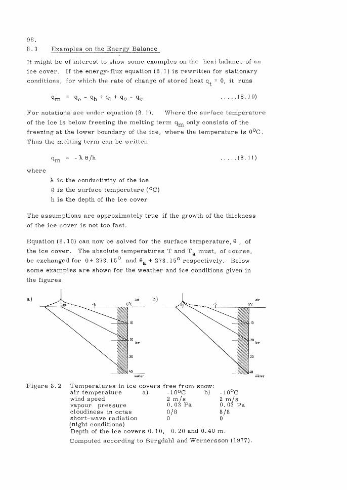
98.
8.3 Balance
It might be of interest to show some examples on the heat balance of an
ice cover. If the energy- flux equation (8. 1) is rewritten for stationary
conditions, for which the rate of change of stored heat qt 0, it runs
..... (8.10)
For notations see under equation (8. 1). \!\There the surface temperature
of the ice is below freezing the melting term qm only consists of the
freezing at the lower boundary of the ice, where the temperature is OOC.
Thus the melting term can be written
where
A is the conductivity of the ice
8 is the surface temperature (OC)
h is the depth of the ice cover
..... (8.11)
The assumptions are approximately true if the growth of the thickness
of the ice cover is not too fast.
Equation (8.10) can now be solved for the surface temperature, 8 , of
the ice cover. The absolute temperatures T and Ta must, of course,
be exchanged for 8+ 273.150. and 8a + 273.15 0 respectively. Below
some examples are shown for the weather and ice conditions given in
the figures.
a) b)
Figure 8.2
water water
Temperatures in ice covers free from snow: air temperature a) -100C b) wind speed 2 m Is vapour pressure 0.03 Pa cloudiness in octas 0/8 short-wave radiation 0 (night conditions)
-10 0 C 2 m/s 0.03 Pa 8/8 o
Depth of the ice covers 0.10, 0.20 and 0.40 m.
Computed according to Bergdahl and Wernersson (1977).
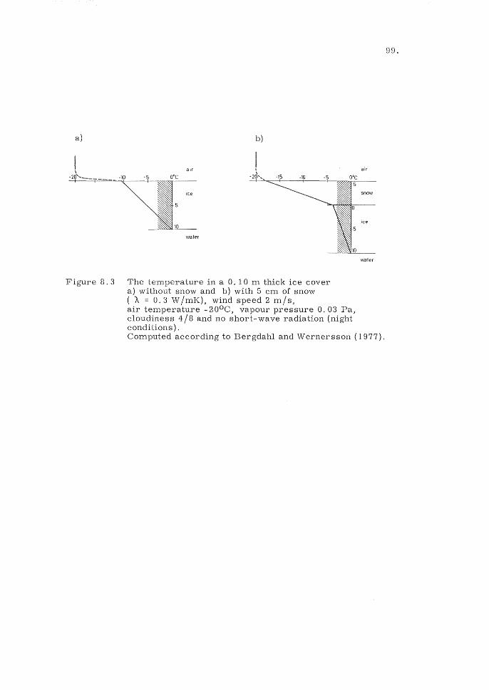
a) b)
water
Figure 8.3 The temperature in a 0.10 m thick ice cover a) without snow and b) with 5 cm of snow ( A = 0.3 W /mK), wind speed 2 m/s, air temperature 20oC, vapour pressure 0.03 Pa, cloudiness 4/8 and no short-wave radiation (night conditions) .
air
water
Computed according to Bergdahl and Vvernersson (1977).
99.

100.
9 MECHANICAL PROPERTIES
Natural ice shows many peculiar properties, distinguishing it from
other materials, and it is most important to bear this in mind when
studying the mechanics of ice or when using values of ice strength for
design purposes.
9.1 Considerations
Ice is a crystalline material with very coarse crystals compared to
for example steel. The ice crystals also vary widely in size. The
diameter is of the order of 10- 3 m in snow ice and can be of the order
of 10- 1 m in columnar fresh-water ice. See chapter 2.
Furthermore, the ice crystals have an anisotropic structure, and the
orientation of the c-axis varies from one crystal to another. In colum
nar sea-ice the crystals have a preferred orientation (horizontal c":'axes),
in columnar fresh-water ice the preference is weaker, and in snow ice
there is a completely random orientation of the axes.
Polycrystalline ice usually contains impurities e. g. air bubbles, salts,
organic or inorganic matter. In fresh-water ice most of the impurities
are concentrated to the crystal boundaries. In a saline sea, on the
other hand, the brine is mostly contained within the ice crystals between
the platelets. See paragraph 2. 52.
The coarse texture of ice is the reason why samples of ice, of the same
size, contain parts of one, two, three or several crystals with different
orientations and, of course, this fact influences the values of measured
quantities. See figure 9. 1 .
b c
Figure 9. 1 Dependence of properties of ice on its structure.
101.
Another consequence of the coarse texture of ice is that ice strength
values are strongly dependent on the size of the samples, as the num
ber of contained crystal boundaries and crystal defects increases with
size. For fine- grain materials, like steel, this effect becomes apparent
only for samples with very small dimensions such as strings and slen
der axles. This so called scale effect is treated in paragraph 9. 6.
Because of all these factors the observed mechanical properties of
ice show a large scatter in values even if samples are taken from
nearby parts of a large ice field.
9.2 The Role of
Being a crystalline solid, ice should tentatively show similar mechan
ical properties as for example steel, if one takes into due account the
difference in crystal size. However, ice is generally confronted at
temperatures very close to its melting point.
At such elevated temperatures the mechanics of a crystalline solid is
controlled by thermally activated processes. At temperatures between
50-100% of the absolute melting temperature, T m' the mechanical prop
erties are strongly dependent on strain rate and temperature. For
ice T m = 273 K and as it usually occurs at temperatures above 0.8 T m
(220 K ~ 50 0 C) it is understood that temperature plays an important
role.
Evidence of the thermal activity of ice is the self diffusion of whole
water molecules in the solid, and the strong dependence of the rate
of diffusion on temperature. The diffusion coefficient D can be written
..... (9.1)
where
Do = (9. 13 ± 0.57) 10-4 m 2 /s
Qs 59.8 kJ /mol; the activation energy for self diffusion
R 8. 31 J / (mol· K) = the universal gas constant
T the absolute temperature.
The diffusion coefficient D is used as a parameter in the creep models
presented in paragraph 9.32. (Ramseier, 1967a, b).
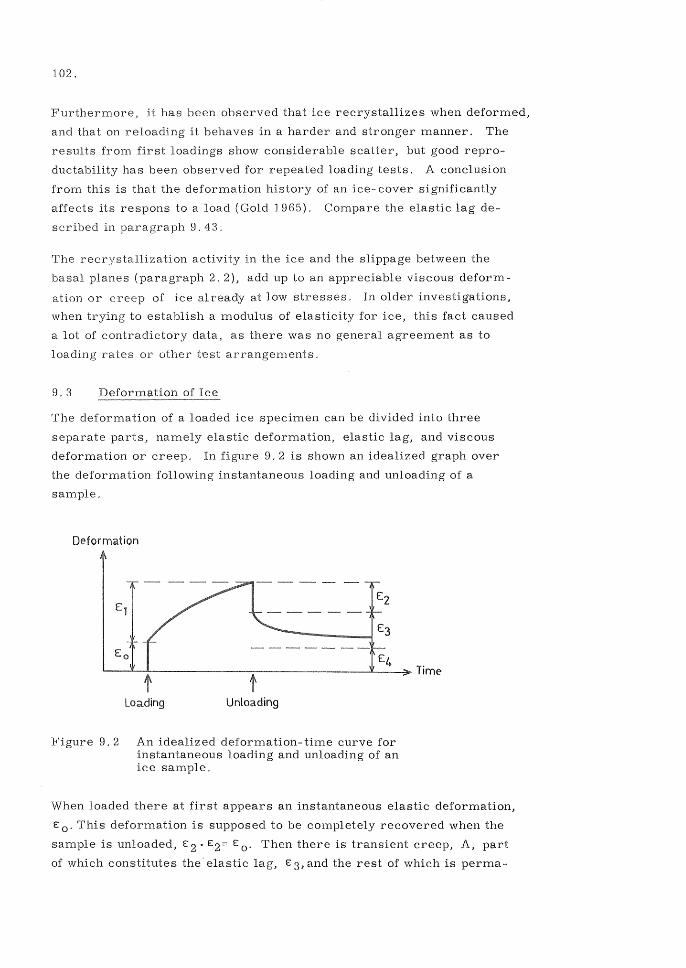
102.
Furthermore, it has been observed that ice recrystallizes when deformed,
and that on reloading it behaves in a harder and stronger manner. The
results from first loadings show considerable scatter, but good repro
ductability has been observed for repeated loading tests. A conclusion
from this is that the deformation history of an ice- cover significantly
affects its respons to a load (Gold 1965). Compare the elastic iag de-
scribed in 9.43.
The
basal
~ClJLLL"-'Cl~.L\ .. 'H activity in the ice and the slippage between the
(paragraph 2.2), add up to an appreciable viscous deform-
ation or creep of ice at low stresses. In older investigations,
when trying to establish a modulus of elasticity for ice, this fact caused
a lot of contradictory data, as there was no general agreement as to
loading rates or other test arrangements.
9.3 Deformation of Ice
The deformation of a loaded ice specimen can be divided into three
separate parts, namely elastic deformation, elastic lag, and viscous
deformation or creep. In figure 9. 2 is shown an idealized graph over
the deformation following instantaneous loading and unloading of a
sample.
Deformation
E4 b---~~--------------~----------------L---~Time
t Unloading
Figure 9.2 An idealized deformation-time curve for instantaneous loading and unloading of an ice sample.
When loaded there at first appears an instantaneous elastic deformation,
Eo. This deformation is supposed to be completely recovered when the
sample is unloaded, E 2 . E2= Eo. Then there is transient creep, A, part
of which constitutes the elastic lag, E 3, and the rest of which is perma-

103.
nent viscous deformation, E 4' E 3 + E4 = El' The elastic lag is supposed
to be recovered after some time.
A rheological model describing such a behaviour could be constituted
of a spring, representing the elastic deformation, in series with a
dashpot, representing the permanent viscous deformation, and a Voight
(or Kelvin-) unit, representing the elastic lag. The Voight-unit is a
dashport in parallel with a spring. See figure 9. 3
Spring Oashpot
Maxwell unit Voight -or Kelvin unit
Figure 9. 3 A composite rheological model of ice. 0 is the load stress, El and E2 are elastic moduli, and 1J 1 and 112 are viscosity moduli.
9.31 Models
If a rheological model is constituted by springs and dashpots with con
stant moduli of elasticity and viscosity, the mathematical formulation
of its deformation will give rise to ordinary partial differential equa
tions. with constant coefficients. The model shown in figure 9. 3 will,
for example, yield
..... (9.2)
where E is the strain and G the stress . and .. denote the first
and second time derivatives respectively.
The solution of such a differential equation is easily performed with
the help of hereditary integrals for any time history of load or deform
ation. The technique is founded on the fact that the solution of the
linear equation for a varying stress can be had by superposing sol-
104.
utions where the stress is considered constant for infinitely short
time intervals.
The deformation E under a constant stress 0 0 applied for t > 0 is
given by
°oJ(t) ..... (9.3)
where J(t) is characteristic for each linear model. It is a monot
tonously increasing function for t > 0, for t < 0 J(t) == O. It is
called the creep compliance.
In the same manner a constant deformation Eo applied for t > 0 will
yield the force
o (t) = Eo Y(t) ..... (9. 4)
where Y(t) is called the relaxation modulus and is, at least, a non
increasing function of time.
The superposing of load increments do at their corresponding times
and integrating equation (9.3) gives the hereditary integral
t=1: J E(t) =t=O J(t-1:) do (1:) ..... (9.5)
The technique is described in for example Fliigge: Viscoelasticity (1975),
where also the creep compliance and relaxation modulus are given for
some rheological models.
The linear model of equation (9.2) has been used for sea ice by
Tabata (cited by Weeks and Assur 1967) and by Lindgren (1968) for
columnar fresh-water ice. Both scientists tried to evaluate their
experiments in terms of moduli independent of strain rate and
stress. It was, however, found that especially the viscosity modulus
1) 1 is strongly dependent on stres s and strain.
Jumppanen (1973) calculated the pressure against the walls of water
reservoirs by evaluating the creep compliance, J(t), directly from experi
ments. In his experiments he found that for 0.7 MPa the ice showed
weak nonlinearity and for 1. 2 MPa strong nonlinearity. For a stress
greater than 1 MPa the linear rheological model will thus give an
inadequate description of deformation or stress.

105.
9.32 A Nonlinear LL~H::;\JiLJC"_LClLi Model
Because of the limitations of the linear rheological model above other
approaches have been made by for example Glen(1958), Ramseier
(1971) and Drouin et Michel (1971), making use of the similarities be
tween the deformation of ice and other crystalline solids.
These authors disregard the elastic lag and use models with a linear
spring in series with a nonlinear dashpot. See figure 9.4.
Linear spring Nonlinear dashpot
Figure 9.4 A nonlinear rheological model of ice. E is an elasticity modulus. K, D and n is defined by equation 9. 5
For constant temperature the equation of the proposed model can be
written
E o + KD ( Ci /E)n E ..... (9.6)
where K and n are functions of strain, strain rate, and stress. D is
the self-diffusion coefficient for the water molecules in ice.
Neither the linear nor the proposed nonlinear model can give a com
plete picture of the deformation of ice because of the complexity of
its structure and deformation. The linear model has four parameters
who actually cannot be considered constant for but narrow intervals
of stress and strain. The described nonlinear model has three para
meters. The product KD can be considered as one. Experimental
curves are easier to fit but still the parameter constants must be
changed for one mode of deformation to another, see paragraph 9.44.
It should be stressed that all constants in this chapter are functions of
temperature, type of ice, the angle between load and crystal axes
and type of load (tension, bending, compression). The separate parts
of the models are treated in the following paragraphs.
106.
9.4 Fresh-Water Ice
If one looks at the rheological models for ice described in the pre
vious paragraphs it is understood that the values on the different
model parameters are very sensitive to test arrangements. The
elastic modulus, for example, is often calculated on deformation
that includes some creep. For great stresses the creep can consti
tute a considerable part of the deformation, 'and it must be measured
extremely quickly after the application of the stress. If the time
between load and measurement varies, the value on the elasticity
will, of course, also vary although the "true" property does not.
As discussed above the values on the modulus of elasticity varies
due to the used test method. But the desired magnitude of the modulus
also depends on how it is to be used. If, for example, a pure elastic
model shall be applied on the deflexion of an ice cover under a con
centrated load, it is advisable to use rather low values that include
reasonable viscous deformation. Otherwise, the deflexions will be
grossly underestimated.
!?1~.E1J~ ~la~~i~~L
The most reliable results on the dynamic modulus of elasticity (El
of figure 9.3 or E of figure 9.4) are received from seismic methods
measuring the speed of the propagation of sound. The phase speed
of the compression wave is~ El / p,' where p is the density of the ice.
The load rate is fast enough that the creep can be disregarded, and
the true elasticity or the tangent modulus at the origin is actually
measured.
By separating compression and shear waves, which have different
phase velocities it is also possible to get the elastic shear modulus or
the Poisson modulus.
For natural lake ice Boyle et Sproule and Northwood, cited by Pounder
(1965), found that the elastic modulus was independent of crystal
orientation. Their values also agree well with results by Frolov et
Slesarenko (1972), Ewing, Berdennikov, Serikov, Bogorodskii and
Lavrov all cited by Lavrov (1969). Taking Bogorodskii''' s results
for ice with almost no bubbles the elastic modulus as a function of
107.
temperature Q could be written:
El = (1 - cQ) . 8.4 GPa ..... (9.7)
where c = O. 011 oe- 1 . All results reported by the cited scientists
lie within 1- 10% of this expression in the interval - 30 0 e .::s;: Q ~ ooe.
It should be pointed out that the elasticity of turbid ice or deteriorating
spring ice may be only 300/0 of that given by equation 9.7.
In compression tests, when applying either one of the models, there
is inevitably a lot more scattered results. One reason for this is
the inclusion of a part of the viscous deformation. Another reason
is that each specimen contains only a few crystals whose orientation
can vary widely, see figure 9. 1 page 101. A third reason is the
difficulty to get flawless specimens and the fact that the more crys
tal boundaries per specimen the lower elasticity. See the scale
effect para.graph 9.6. In the seismic tests, local irregularities or
faults play little role as they occupy only a small fraction of the
tested volume. Often the measurements are made on ice- fields
in situ.
Experiments by Lindgren (1968) and Gold (1968), performed on col
umnar fresh-water ice (SI) with the stress applied perpendicular to
the growth direction, are in good agreement with each other, and
the expression (9. 8) is a reasonable approximation of their results
holding in mind that the standard deviation of, for example, Lind
gren's values are 0.8 GPa.
E = (1 - c Q) . 6.1 GPa ..... (9.8)
where c = O. 012 oe -1 .
For snow ice (T1) and granular shelf ice Ramseier (1971) proposed
E = (1 - c Q) • 5. 1 GPa ..... (9.9)
where c = 0.012 °e- 1
For ice monocrystals Gold (1958) found that the modulus of elasticity
was not a function of temperature, and the elasticity parallel to or
perpendicular to the c-axis was found to be 8.3 GPa. It appears

108.
therefore, that the fairly large variation with temperature of the
static elastic modulus of polycrystalline ice is due to the tempera
ture dependence of grain boundary slip.
The elastic modulus of ice shows different values for compression
and tension. For "structurally simulated" ice Lavrov (1969) re
ceived a secant modulus of elasticity of 1. 3 GPa in compression
and 0.12 GPa in tension. (Structurally simulated ice is ice seeded
with hoar-frost crystals in the moment of formation. In this way
an ice cover is made with columnar structure and with extremely
small diameters of the columns). The duration of load action
was 13 s and thus the modulus included some viscous deformation.
Johnson (1972), who re examined sea ice data by Peyton (1966),
concluded that the secant modulus in tension was five to ten times
that in compression. The modulus varied with crystal orientation
and compressive strength of the samples. The modulus in tension
was approximately 7 GPa and in compression 1.4 GPa (sic). The
relations are thus quite contradictory.
Generally, the secant modulus in tension is 5 ± 4 GPa for columnar ice
(SI). 5 GPa is assigned by Lavrov (1969) for moderate load duration
(4 s) but, of course, higher values are received for shorter duration
and lower for longer duration of load action.
The elastic modulus for bending is the most investigated property of
ice. According to the theory of strength of materials the modulus
received in bending tests, assuming the beams to have a constant elas
ticity, is a reduced modulus, E b , which combines the moduli in com
pression, E c ' and tension, Et:
.... , (9.10)
Published bending test values show great differences, but it has re
cently been shown by Lavrov (1969) that the values received in bending
tests are due not only to ice structure, temperature and load duration
but also to sample dimensions. This is an example of the scale
effect which is discussed in paragraph 9. 6.
9.42 The Poisson Modulus
For dynamic tests Lavrov (1969) reported the Poisson modulus V to

109.
O. 35 "±" O. 04. In compression tests measured values of the Poisson
modulus vary widely due to the complicated pattern of crystals in
the samples. See figure 9. 1. La vrov reported values varying be
tween 0.0014 and 2.66.
Note that for pure viscous deformation the modulus is 0.5, and for
creep tests with isotropic and homogeneous samples the Poisson mod
ulus should approach this value. Drouin et Michel (1971) verified this
in experiments with snow ice.
9.43
Studying the creep of ice by means of a constant load test it. is possible
to distinguish three stages of creep. Typical creep curves in tension
at different temperatures are depicted in figure 9. 5, where the inital
increase of the true creep strain to Eo can be considered as the
elastic deformation. The part between Eo and El is called primary
or transient creep. In this stage the substructure changes and the
creep rate is strongly dependent on the creep stress but in a minor
way on temperature. From E 1 to E 2 secondary or steady state creep
develops, where the rate of deformation is constant and the substruc
ture remains practically unchanged. Finally, in the last stage the
creep accelerates, the specimen necks, voids are formed near the
grain boundaries, and cracks develop leading to a tensile creep
failure.
For secondary creep there is a relation between strain rate and stress
but for tertiary or primary creep no such relation has been proposed.
Constant stress temperature T1< T2 < T3
3rd Stage (terti;uy creep)
creep)
1st Stage (primary creep)
Time ,s
t
5-105
Figure 9. 5 Typical creep curve in tension depicting three stages of creep using a constant load but at different temperatures. After Ramseier (1971).
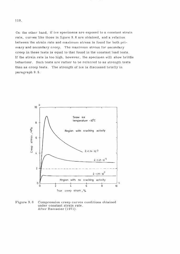
110.
On the other hand, if ice specimens are exposed to a constant strain
rate, curves like those in figure 9.6 are obtained, and a relation
between the strain rate and maximum stress is found for both pri
mary and secondary creep. The maximum stress for secondary
creep in these tests is equal to that found in the constant load tests.
If the strain rate is too high, however, the specimen will show brittle
behaviour. Such tests are rather to be referred to as strength tests
than as creep tests. The strength of ice is discussed briefly in
paragraph 9.5.
C1l a.. :2
III III
~ if}
n. <IJ <IJ
U
o 10
8
6
4
2
Snow ice temperature -WoC
Region with cr(;lcking activity
E: = 1.24· 10-3
. -5 E=1.47'lO
• -7 E=1.77·10
Region with no cracking act ivity o L-______ -+ ________ +-______ ~--------~------~ E
o 2 4 6 8 10
True creep strain J %
Figure 9.6 Compression creep curves conditions obtained under constant strain rate. After Ramseier (1971).
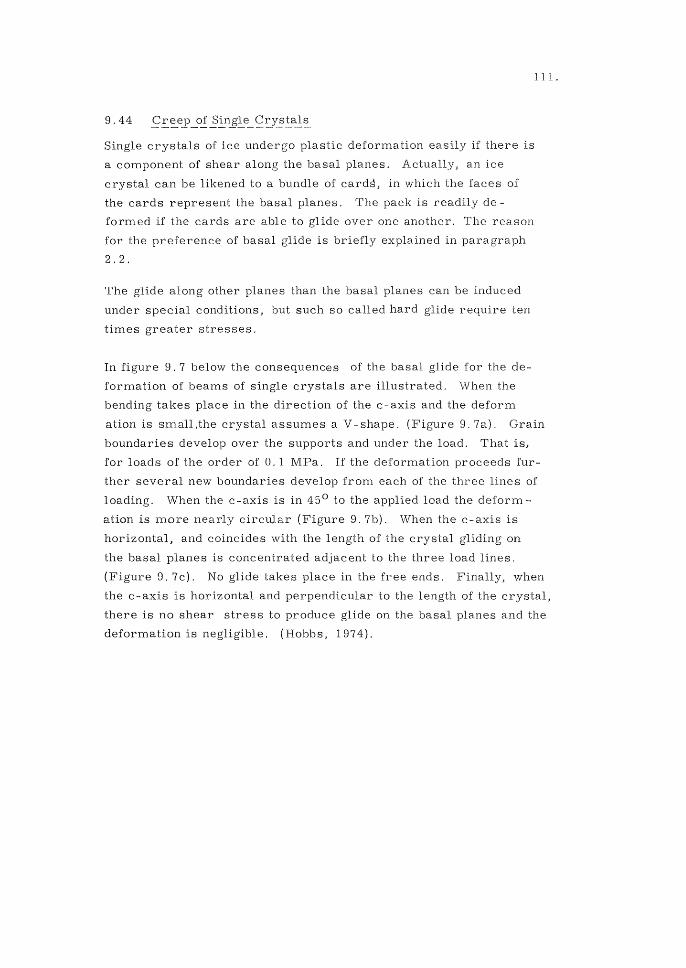
Single crystals of ice undergo plastic deformation if there is
a component of shear along the basal planes. Actually, an ice
crystal can be likened to a bundle of card~, in which the faces of
the cards represent the basal planes. The pack is readily de -
formed if the cards are able to glide over one another. The reason
for the preference of basal glide is briefly explained in paragraph
2.2.
The glide along other planes than the basal planes can be induced
under special conditions, but such so called hard glide require ten
times greater stresses.
In figure 9. 7 below the consequences of the basal glide for the de
formation of beams of single crystals are illustrated. \iVhen the
bending takes place in the direction of the c-axis and the deform
111.
ation is small,the crystal assumes a V-shape. (Figure 9. 7a). Grain
boundaries develop over the supports and under the load. That is,
for loads of the order of O. 1 MPa. If the deformation proceeds fur
ther several new boundaries develop from each of the three lines of
loading. When the c-axis is in 45 0 to the applied load the deform
ation is more nearly circular (Figure 9. 7b). \iVhen the c-axis is
horizontal, and coincides with the length of the crystal gliding on
the basal planes is concentrated adjacent to the three load lines.
(Figure 9. 7c). No glide takes place in the free ends. Finally, when
the c-axis is horizontal and perpendicular to the length of the crystal,
there is no shear stress to produce glide on the basal planes and the
deformation is negligible. (Hobbs, 1974).
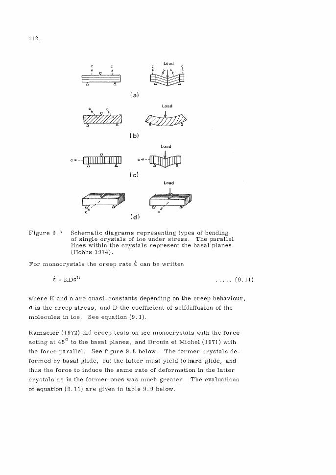
112.
Load
(a)
Load
Load
Load
Figure 9. 7 Schematic diagrams representing types of bending of single crystals of ice under stress, The parallel lines within the crystals represent the basal planes, (Hobbs 1974),
For monocrystals the creep rate E can be written
.. ,., (9,11)
where K and n are quasi-constants depending on the creep behaviour,
(j is the creep stress, and D the coefficient of selfdiffusion of the
molecules in ice. See equation (9. I),
Ramseier (1972) did creep tests on ice monocrystals with the f9rce
acting at 45 0 to the basal planes, and Drouin et Michel (197J) with
the force parallel. See figure 9. 8 below. The former crystals de
formed by basal glide, but the latter must yield to hard glide, and
thus the force to induce the same rate of deformation in the latter
crystals as in the former ones was much greater. The evaluations
of equation (9,11) are given in table 9,9 below,

Figure 9.8
Table 9.9
EjD (m- 2)
The deformation of two monocrystals with different orientation of crystal axes. The left crystal exhibit basal glide and the right one hard glide along the marked planes. The parallel lines within the crystals represent the basal planes.
113.
Ice monocrystals the stress at 45 0 to the basal planes. Values of the constants K and n in equation 9. 11 for ~wo ranges of temperature compensated creep rate, EjD. Rarrtseier (1972).
n
109 _ 6.21.1010
6.21.10 10 - 4.9.1012
K(m- 2pa- n )
1.560.10- 2
4.49.10- 7 1. 712
2.329
Table 9. 10 Ice monocrystals the stress parallel to the basal planes.
E/D (m- 2 )
2.107 - 8.109
Values of the constants K and n in equation 9. 11. Calculated on data from Drouin et Michel (1971).
K(m- 2pa- n )
4.40.10- 16
n
3.651
The function (9. 11) is illustrated in figure 9. 12 in the next paragraph
with the constants from table 9. 9 and 9. 10. It is clearly seen that in
the common interval of E /D the deformation due to easy glide is ten
fold faster than the deformation due to hard glide.
114.
9. 45 ~£~eJ>_ol~~!Y~£.LsJ:~lli~~lc~
The deformation of polycrystalline ice is composed of the basal
glide within the crystals, of grain- boundary sliding and of liquid
water at triple junctions caused by stress concentrations at these
points. Below -10 oe the basal glide is dominating. Because of
the varying orientation of the grains in polycrystalline ice, the
rate of flow is much smaller than for basal glide of ice monocrys
tals. Some grains are forced to deform by hard glide because of
their orientation. Above -10oe the creep of polycrystalline ice is
dominated by the grain boundary sliding and the melting at triple
joints due to the stress concentrations caused the sliding.
Most experiments on the creep of polycrystalline ice have been
made with snow ice or nucleated columnar ice with small diameter
of the grains. Experiments with such ice give good reproducta
bility, because there are enough grains in a specimen to give reli
able bulk properties. If, however, a specimen contains only a few
grains, as would be the case with an ordinarily sized specimen
from a lake ice cover, the shifting orientation from specimen to
specimen would give experimental results that showed vast scatter.
See figure 9. 1.
Ramseier (1971) and Drouin et Michel (1971) gave the creep rate of
polycrystalline ice in secondary creep (see figure 9. 5) as
n E KD (~
where K and n are quasi- constants and functions of the creep be
haviour, 0 the maximum stress, E the elastic modulus and D the
coefficient of selfdiffusion of the molecules in ice. D and E are
both functions of temperature. xl
(9.12)
Equation (9. 12) combined in series with an appropriate elastic mem
ber to a nonlinear rheological model (see figure 9.4) will good
fit to curves within the no- cracking region in figure 9. 6. Within the
region with cracking activity, however, the maximum stress will be
somewhat delayed and furthermore the stress will not decrease with
time as it should.
xl Later R~mseier and Dickins (1972) have modified the equation (9.12) for polycrystalline ice to
E DA(sinh (aOIE))n
where a, n a~d A are constants throughout the whole range of deformation:2.10 2< E/D< 2.10 13 m- 2 , on the other hand it will give a fourparameter model. F·or small values on ao lE it approaches (9. 12).
115.
Drouin et Michel (1971) have succeeded in making a better fit to con
stant strain rate curves by using dislocation theory. Taking into
account the number of edge dislocations (see figure2. 9b) and their
increase in number with the deformation, e:, they end up with the
expression
E: = 2 b (no + ..... (9.13)
where b is Burgers vector (see paragraph 2.2), no is the original
number of dislocations per unit area, and ~ the rate of increase of
dislocations. b and are constants for all types of hexagonal ice.
13 varies with the type of ice and p is both a function of temperature
and the type of ice. The equation is dimensionally incorrect. Combined
with an elastic member to a rheological model it will give a four-para
meter model W, p, n, E), while the use of equation (9.12) will result
in a three-parameter model (K, E, n).
If one applies equation (9. 13) to the case with the constant load, Ci
it is evident that it will yield an accelerated creep also for primary
and secondary creep, which is not the case. See figure 9.5, which
agree with experiments bye. g Lindgren (1968) and Lavrov (1 969).
One can therefore not state that equation (9.13) is superior to the
more common and more easily used creep rate function (9.12).
The constants K and n of equation (9. 12) is given for snow ice in table
9.11 below. For columnar ice covers there are some experiments that
justify the use of the constants for uniaxially loaded monocrystals,. t<'.l.ble
9. 10, also for biaxially restricted plates containing several crysta:.s.
This may be explained by the fact that it is not possible that all crys
tals have a vertical orientation in a natural ice cover. For seeded ice
covers or columnar ice covers with horizontal optical axes (S2) the
pressure in expansion tests "vas found not to exceed the pressure in
ordinary (SI) ice covers. (See Bergdahl 1978).
Table 9.11
sjD (m -2)
<0.7.106
0.7.106 -
109 _ 1013
Snow ice (T1). Values of the constants K a.nd n of equation (9. 12) for different ranges of temperaturecompensated creep rate € ID 1) calculated from figure of Rams eier (1971) founded
on data from Butkovich and Landauer 2) Ramseier's (1971) own results
K (m- 2) n
8.47.1010 1.148 1 )
10 9 4.712 . 10 19 3.118 2)
1.297.1027 5.27 2)
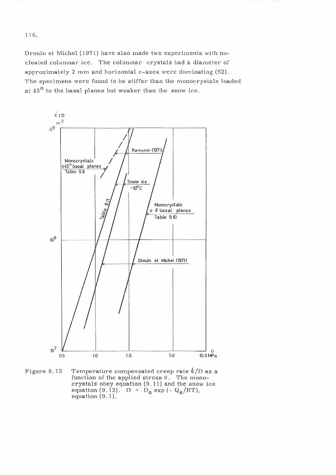
116.
Drouin et Michel (1971) have also made two experiments with nu
cleated columnar ice. The columnar crystals had a diameter of
approximately 2 mm and horizontal c-axes were dominating (82).
The specimens were found to be stiffer than the monocrystals loaded
at 45 0 to the basal planes but weaker than the snow ice.
Figure 9.12
Monocrystals I 045 0 basal planes ,I
Table 9.9 ;'
1.0 2.0
Monocrystals o 11 basal planes
Table 9.10
Drouin et Michel (19711
5.0 o
10.0 MPa
Temperature compensated creep rate E ID as a function of the applied stress o. The monocrystals obey equation (9.11) and the snow ice equation (9.12). D = Do exp (- Qs/RT), equation (9. 1).
9.46 Activation and Self Diffusion
Experimental results on the creep rate of ice can be brought into
coincidence by using the function
117.
E: = f(o) exp (- Qc/RT) ..... (9.14)
where Qc is the activation energy for creep
o the applied stress
R the universal gas constant
T the absolute temperature
For a large number of metals and components it has been shown
that Qc and the activation energy for self diffusion Q s should be
approximately equal. Q s is a constant in the equation for self
diffusion (9. 1):
The activation energy of creep Qc can be calculated from 9. ] 4, if
the creep rate is known at two different temperatures for the same
load.
d(ln E: ) - R ..... (9. 15)
d (1 IT)
Now, if one takes the logarithm of and differentiates equation (9.12),
which is the experimentally established function for (9. 14), the
following result of the differentiation with respect to (1 IT) is had
d + n --'-----'-d (liT)
Inserting this result into (9. 15) the first term can be identified as
the activation energy for self-diffusion. Q s according to equation
(9. 1), and thus
..... (9.16)
This result is interesting in two ways. First, for monocrystalline
ice the elasticity E is not a function of temperature so that the
activation energies for creep and self-diffusion ought to be equal.
Secondly, for polycrystalline ice the elasticity decreases with
118.
temperature, that is dE/dT < 0, and consequently the activation
energy for creep is greater than the activation energy for self
diffusion.
The result mirrors the different deformation behaviour of poly-
and ice. In the former ice the creep
and at the boundaries play a considerable role but in
monocrystals there is, of course, only creep within the crystal
structure.
Drouin and Michel (1971) found in their experiments with mono
basal
59.8
that in tests with the stress applied parallel to the
60.7 kJ /mol which is nearly equal to Q s =
For snow ice below 4 0 C received Qc ~ 83 kJ /mol and n = 4.
VVith the values listed below equation (9.16) yields 84. 5 kJ /mol.
R 8.31 J /(mol K)
T 263.15 K (-10 0 C)
E 5.71 GPa (eq. 9.9)
dE / dT O. 061 2 (eq. 9. 9) .
9.47
Structurally unhomogeneous materials show so called elastic lag
or delayed elasticity, that is, when a specimen of such a material
is unloaded some of the deformation is recovered after some time,
see 9.2, paragraph 9.3.
For an ice that contains grains of different orientation,
the phenomenon can be as follows. Some grains, like
grains 1 and 3 in figure 9. 13, creep by easy glide and after a
short duration of load a great part of their deform-
ation is viscous deformation. Other grains, like
grain 2 in figure 9. 13, respond to the load by almost only elastic
deformation, while the creep by hard glide is . rather slow. The
stress in the U'l>'L..LLU<-U could. be distributed like the
nVDoltnet:lc~H distribution of figure 9. 13b. When unloaded the
stress cannot disappear immediately but will be balanced inter
nally, so that the expansion of the stiff grain (2) is restricted
by the more deformed weak grains (], 3). The resulting stress
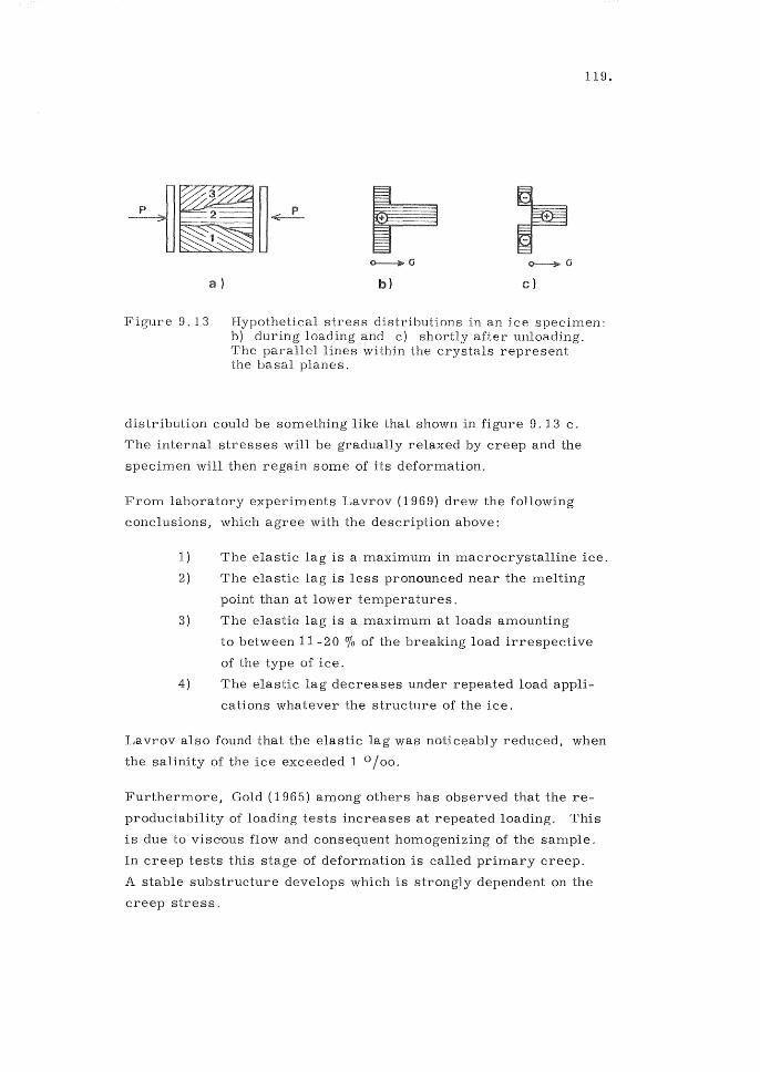
119.
(j
Figure 9.13 Hypothetical stress distributions in an ice specimen: b) during loading and c) shortly after unloading. The parallel lines within the crystals represent the basal planes.
distribution could be something like that shown in figure 9. 13 c.
The internal stresses will be gradually relaxed by creep and the
specimen will then regain some of its deformation.
From laboratory experiments Lavrov (1969) drew the following
conclusions, which agree with the description above:
1) The elastic lag is a maximum in macrocrystalline ice.
2) The elastic lag is less pronounced near the melting
point than at lower temperatures.
3) The elastiG lag is a maximum at loads amounting
to between 11 -20 % of the breaking load irrespective
of the type of ice.
4) The elastic lag decreases under repeated load appli
cations whatever the structure of the ice.
Lavrov also found that the elastic lag was noticeably reduced, when
the salinity of the ice exceeded 1 0/00.
Furthermore, Gold (1965) among others has observed that the re
productability of loading tests increases at repeated loading. This
is due to viscous flow and consequent homogenizing of the sample.
In creep tests this stage of deformation is called primary creep.
A stable substructure develops which is strongly dependent on the
creep stress.
120.
U sing the linear rheological model of figure 9. 3 (page 104) where
the Voight-unit represents the elastic lag Tabata (1958) studied
beams of sea ice and Lindgren (1968) columns of fresh-water
ice. Because the columns contain only a few crystals each and
because of the inhomogeneity of the sea ice beams there was bound
to be a vast scatter of the elastic-lag constants E2 and 112' Lind
gren found for fresh-water ice
3.4 GPa <E2 < 14 GPa}
112 ~ 1013 Ns/m2 Q
..... (9.17)
and Tabata found for sea ice
..... (9.18)
The latter also found that in situ beams of sea ice showed less
elastic lag when deflected horizontally than vertically.
9.48 Relaxation Times
The behaviour of an ice specimen after an instantaneous unloading
can be described by, for example, the linear model equation (9.2)
which with G 6 = G = 0 and integrated twice gives
where
£ £3 exp (- E2 t/112) + £4
£ is the deformation for t > 0
t the time
E 2, 1\2 the constants of delayed elasticity
£ 3 the elastic lag
£4 the permanent viscous deformation
£3 + £4 the initial deformation at t = 0+
see figure 9. 2 page 103.
..... (9.19)
The time when the exponent of e in equation (9. 19) equals -1 is
called the relaxation time and it can be used as a measure of the
time scale of the elastic lag. The relaxation time thus equals
the quotient 112/E2' Using Lindgren' s values (9.17) it is found
to be of the order of 103 s for fresh-water ice and Tabata" s values
(9.18) give the same order of magnitude for sea ice.
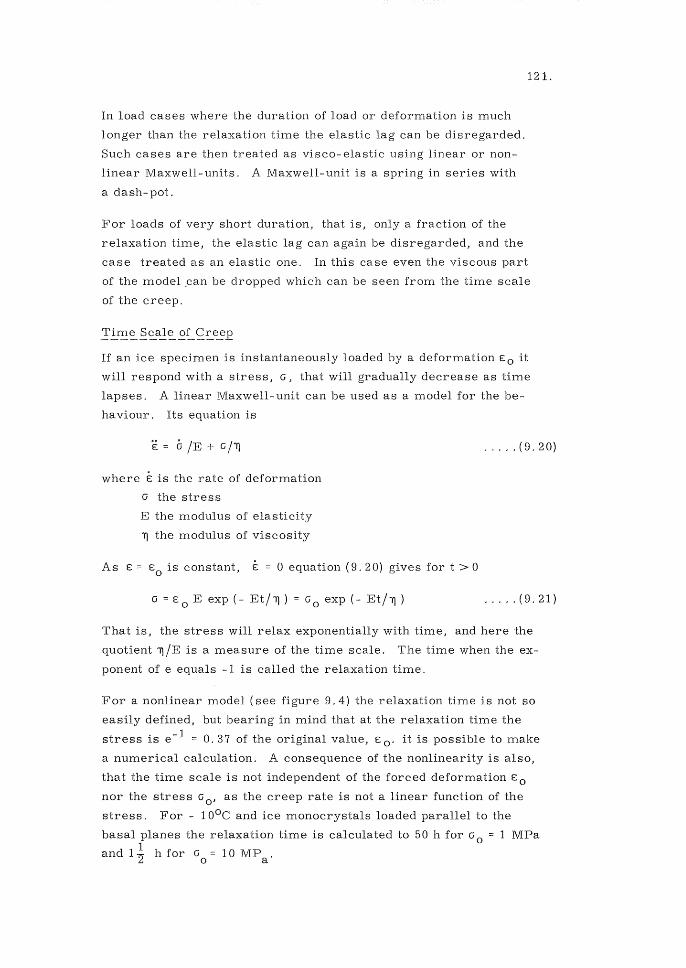
In load cases where the duration of load or deformation is much
longer than the relaxation time the elastic lag can be disregarded.
Such cases are then treated as visco-elastic using linear or non
linear Maxwell-units. A Maxwell-unit is a spring in series with
a dash-pot.
121.
For loads of very short duration, that is, only a fraction of the
relaxation time, the elastic lag can again be disregarded, and the
case treated as an elastic one. In this case even the viscous part
of the model .can be dropped which can be seen from the time scale
of the creep.
Time Scale of
If an ice specimen is instantaneously loaded by a deformation Eo it
will respond with a stress, G, that will gradually decrease as time
lapses. A linear Maxwell-unit can be used as a model for the be
ha vi our . Its equation is
E 0 lE + G 111
where E is the rate of deformation
G the stress
E the modulus of elasticity
11 the modulus of viscosity
As E = Eo is constant, E = 0 equation (9.20) gives for t > 0
G = E 0 E exp (- Et 111 ) = Go exp (- Et 111 )
..... (9.20)
..... (9.21)
That is, the stress will relax exponentially with time, and here the
quotient i1IE is a measure of the time scale. The time when the ex
ponent of e equals -1 is called the relaxation time.
For a nonlinear model (see figure 9.4) the relaxation time is not so
easily defined, but bearing in mind that at the relaxation time the
stress is e- 1 = 0.37 of the original value, Eo' it is possible to make
a numerical calculation. A consequence of the nonlinearity is also,
that the time scale is not independent of the forced deformation Eo
nor the stress Go' as the creep rate is not a linear function of the
stress. For - 100 e and ice monocrystals loaded parallel to the
basal planes the relaxation time is calculated to 50 h for Go 1 MPa 1
and 12" h for Go = 10 MP a'
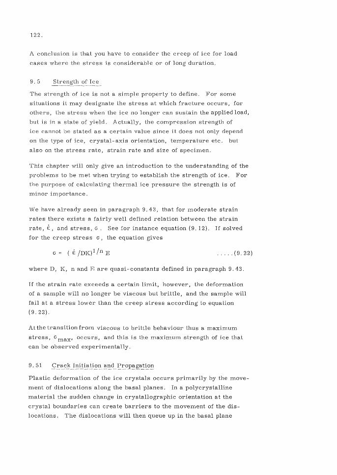
122.
A conclusion is that you have to consider the creep of ice for load
cases where the stress is considerable or of long duration.
9.5 of Ice
The strength of ice is not a simple property to define. For some
situations it may designate the stress at which fracture occurs, for
others, the stress when the ice no longer can sustain the applied load,
but is in a state of yield. Actually, the compression strength of
ice cannot be stated as a certain value since it does not only depend
on the type of ice, crystal-axis orientation, temperature etc. but
also on the stress rate, strain rate and size of specimen.
This chapter will only give an introduction to the understanding of the
problems to be met when trying to establish the strength of ice. For
the purpose of calculating thermal ice pressure the strength is of
minor importance.
We have already seen in paragraph 9.43, that for moderate strain
rates there exists a fairly well defined relation between the strain
rate, E, and stress, G. See for instance equation (9.12). If solved
for the creep stress G, the equation gives
o ( E IDK)l In E ..... (9.22)
where D, K, nand E are quasi-constants defined in paragraph 9.43.
If the strain rate exceeds a certain limit, however, the deformation
of a sample will no longer be viscous but brittle, and the sample will
fail at a stress lower than the creep stress according to equation
(9.22).
At the transition from viscous to brittle behaviour thus a maximum
stress, G max' occurs, and this is the maximum strength of ice that
can be observed experimentally.
Plastic deformation of the ice crystals occurs primarily by the move
ment of dislocations along the basal planes. In a polycrystalline
material the sudden change in crystallographic orientation at the
crystal boundaries can create barriers to the movement of the dis
locations. The dislocations will then queue up in the basal plane
against the boundary, and a concentrated stress is created at the
end of the plane.
123.
This stress may be strong enough to initiate a crack. For moder'
ate stresses it creates melting at these triple junctions. Compare
paragraph 9.45. Complete fracture of the specimen does not
necessarily follow immediately on this crack formation, since the
formation will relax the concentrated stress and the crack will stop
growing unless it becomes self propagating.
Carter (1970) has shown that under a uniaxial tensile load the crack
will spread catastrophically throughout the ice, but under a com
pressive stress the first formed cracks will come to a rest after
a finite length.
9. 52 _:t~~sJ:~YJ:~e.E~1J:l_
In his work Carter (1972) gives a theoretical value for the tensile
strength by 1/2
G = t + 2 1:
o ..... (9.23)
where 1: 0 O. 3 MPa for snow ice and independent of temperature
y 10.9 J 1m2 the surface energy
E the elastic modulus
\) Poisson" s coefficient
and dcr = the grain diameter
Equation (9.23) agrees well with Carter" s (1970) own experimental
data, and also with results by for instance J ellinek (cited by Gold
1968), who for granular ice at OOC received the ultimate tensile
strength to 1.6 MPa. Equation (9.23) gives G t= 2.1 MPa for this
case.
The tensile strength of ice at different temperatures and strain
rates whould then ideally be given by the lowest of the two values
received from equations (9.22) and (9.23) for polycrystalline ice
and from (9.11) and (9.23) for ice monocrystals, if the appropriate
constants are applied.
Equation (9.23) is, however, of limited practical interest as it gives
the highest possible tensile strength for a given type of ice. Other
factors as the contents of voids or impurities in a cross section tend
to decrease the tensile strength drastically. This is illustrated in
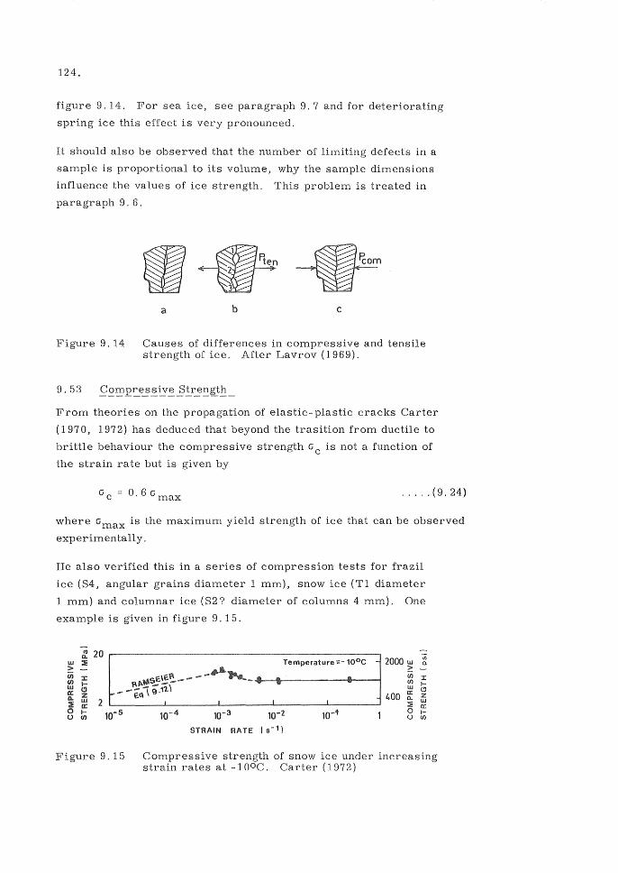
124.
figure 9.14. For sea ice, see paragraph 9.7 and for deteriorating
spring ice this effect is very pronounced.
It should also be observed that the number of limiting defects in a
sample is proportional to its volume, why the sample dimensions
influence the values of ice strength. This problem is treated in
paragraph 9. 6.
Figure 9.14
a b c
Causes of differences in compressive and tensile strength of ice. After Lavrov (1969).
From theories on the propagation of elastic-plastic cracks Carter
(1970, 1972) has deduced that beyond the trasition from ductile to
brittle behaviour the compressive strength Gc is not a function of
the strain rate but is given by
Gc = 0.6 G max ..... (9.24)
where Gmax is the maximum yield strength of ice that can be observed
experimentally.
He also verified this in a series of compression tests for frazil
ice (S4, angular grains diameter 1 mm), snow ice (T1 diameter
1 mm) and columnar ice (S2? diameter of columns 4 mm). One
example is given in figure 9.15.
~ 20 r-------------------------------------------, 2000 W
<f> w :t > (i) J: Cl) IW Cl ex: z Q. W :t ex: o Iu Cl)
Figure 9.15
0. > en :r:: Cl) I-W Cl
400 0::: Z a.. w ~ 0:: 0 t-U Cl)
STRAIN RATE (5- 1 )
Compressive strength of snow ice under increasing strain rates at -1 OOC. Carter (1972)
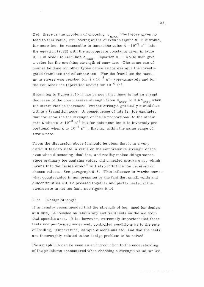
125.
Yet, there is the problem of choosing (imax' The theory gives no
lead to this value, but looking at the curves in figure 9. 15 it would,
for snow ice, be reasonable to insert the value E = 10- 3 s -1 into
the equation (9.22) with the appropriate constants given in table
9. 11 in order to calculate 0max' Equation 9. 11 would then give
a value for the crushing strength of snow ice. The same can of
course be done for other types of ice as for example the investi
gated frazil ice and columnar ice. For the frazil ice the maxi
mum stress was reached for E: 10- 3 s-l approximately and for
the columnar ice (specified above) for 10- 4 s-1.
Returning to figure 9. 15 it can be seen that there is not an abrupt
decrease of the compressive strength from 0max to 0.6 0max when
the strain rate is increased, but the strength gradually diminishes
within a transition zone. A consequence of this is, for example,
that for snow ice the strength of ice is proportional to the strain
rate E: when E: < 10- 3 s-1 but for columnar ice it is inversely pro
portional when E: > 10- 4 s-1, that is, within the same range of
strain rate.
From the discussion above it should be clear that it is a very
difficult task to state a value on the compressive strength of ice
even when discussing ideal ice, and reality makes things worse
since ordinary ice contains voids, old unhealed cracks etc., which
means that the "scale effect" will also influence the received or
chosen values. See paragraph 9. 6. This influence is -maybe some
what counteracted in compression by the fact that small voids and
discontinuities will be pressed together and partly healed if the
strain rate is not too fast, see figure 9. 14.
9.54
It is usually recommended that the strength of ice, used for design
at a site, be founded on laboratory and field tests on the ice from
that specific area. It is, however, extremely important that these
tests are performed under well controlled conditions as to the rate
of loading, temperature, sample dimensions etc, and that the tests
are thouroughly related to the design problem to be solved.
Paragraph 9. 5 can be seen as an introduction to the understanding
of the problems encountered when choosing a strength value for ice
126.
but if specific values are needed, I recommend for instance
Gold'" s (1968) comprehensive paper on the I!Elastic and Strength
Properties of Fresh- Water Icel!. or Butiagin' s (1966) or Lav
rov" s (1969) books.
9. 6 The Scale Effect
Many scientists have found that the measured strength values of
ice are dependent on the size of ice specimens. The reason for
this is as yet not fully understood.
The most wide- spread explanation is that, given a certain density
of different defects in ice, the probability to include some of these
into a specimen increases with the size of the specimen. The fact
that when cutting a big ice block into smaller pieces you are apt to
and sometimes forced to discard defective pieces will, of course,
enhance the strength values of small specimens.
The described theory is mostly referred to as the statistical theory
and it is founded on a general theory of brittle strength developed
by Weibull (1939 a, b) and applied to ice strength by Russian scien
tists, see for example Butiagin (1966) or Lavrov (1969, 1971).
Recently, Hirayama et al (1974) pointed to the fact that the ice
strength should rather be related to the ratio of sample diameter,
d, to crystal size, dcr ' He also found in his experiments that
if this ratio was greater than 25 the ice strength was practically
independent of the sample size. According to him this is consistent
with Butkovich" s (1954) and Butiagin' s tests. Lavrov, on the other
hand, found a relationship between cross sectional area, S, and
compressive strength that holds for d/dcr < 32 or S < 90 cm 2,
dcr = 3 mm
1.9.106 _S-0.20
This function shows a slight decrease in Gc even when d/dcr > 25,
and Lavrov" s conclusion was that an extrapolation should be made
for larger pieces of ice.
For compressive strength it can thus be concluded that the scale
effect can be neglected provided the ice crystals are small com
pared to the tested ice specimens. This is rather easily achieved

127.
for snow ice. For columnar sea ice, where dcr ~ 5 mm, the dia
meter of the specimen must be at least 125 mm. For columnar
fresh-water ice with dcr~ 50 mm one must use field experiments
or resort to some relation like the above equation.
For bending strength, however) the dependence on specimen
volume is not merely caused the random distribution of defects
but also by the low resistance to shear. For further information
see Lavrov (1969).
9.7 of Columnar Sea Ice
In paragraph 2. 52 was decribed how an ice cover developed on a
sea surface. The resulting sea- ice cover consists of columnar
crystals with horizontal c- axes and diameters of approximately
5 mm. It was also stated that the formed ice lattice was pure,
and that brine was trapped in narrow voids within the ice crystals
parallel to their basal planes.
These brine-voids can be shown to be responsible for many
characteristic features of the mechanics of sea ice as well as they
play a great role for the temperature variation of density, conduc
tivity and heat capacity, which has been derived earlier. A crack
in a failed specimen of sea ice, for instance, consists to a con
siderable part of brine voids.
The brine voids are rather regularly shaped and orderly spaced
in the ice. However, the ice also contains trapped air bubbles
which are less orderly arranged and of variable size. Discussing
the thermal expansion of sea ice it was concluded that these air
bubbles were completely separated from the brine voids, which
seemed to be justified in the light of experimental values on the
density of sea ice. As a consequence we disregarded the air
bubbles when calculating the sea ice density as a function of
salinity and temperature. We will not consider them, when
discussing strength or elasticity either, although it has no other
justification than the air- bubble content being rather small com
pared to the brine content.
On the other hand, taking samples in a sea-ice cover and storing
them, makes some of the brine drain off, especially, if the storing
128.
temperature is too high. The total void volume of the ice will,
of course, be related to the original ice salinity. As pointed out
by ·Weeks and Assur (1967) this drained brine volume should be
considered as it sometimes constitutes an appreciable part of
the voids. The brine content by volume of the ice can be calcu
lated with the phase relations given in paragraph 2. 53.
9. 71 Strel2..g!~
A potential failure plane in sea ice only partly consists of ice.
A simple model of sea ice strength would then be to consider the
brine uniformly distributed in the ice and reducing the failure
area by the plane porosity, which in this case equals the volume
porosity or brine content by volume, Vb' Letting G f be the
strength of sea ice and Go the strength of some fictitious brine
free sea ice the following simple relation holds
..... (9.25)
Observe, that the strength, Go' is not the strength of fresh water
ice. The substructure and failure mechanism are too different for
this to hold.
From the strength of materials it is known that near spherical
holes in uniaxially loaded elastic bodies there are stress concen
trations two times the mean stress, and it has been suggested
that the fictitious strength, Go' because of this should be a half
of the strength of fresh water ice of the same temperature, but
fresh-water ice also contains stress risers such as air bubbles
and vapour voids. Furthermore, the failure does not necessarily
start at the voids in fresh-water ice while it mostly does so in
sea ice. (Assur 1958).
As the brine voids are not uniformly distributed in the ice but
concentrated to certain basal planes, potential failure planes
can be situated to cut only a few ice-ice bonds in warm ice, al
though the sea ice still is solid to a considerable part. In cold
ice, however, such a plane is ice to a great extent. The warmer
ice would be expected to have a tensile strength close to zero
even though it contains an appreciable amount of ice. This is
also observed in strength tests, see figure 9.16, where the
ring tensile strength of NaCl ice is drawn as a function of tem-

perature. The extrapolated function gives zero strength for a
brine volume of 70%. For sea ice with the salinity 3 0/ 00 this
corresponds to the temperature - 2 0 C.
If :::E
.c "Ol c: ~ Vi
~ .;;; c: ~
C1l c:
0::
Figure 9.16
3.0
2.0
1.0
0
°
0
°0
0.1 0.2 0.3 0.4 0.5
1/2 Vb I Average brine volume]
A verage ring tensile stress versus square root of the average brine volume, NaCl-ice. (Weeks 1963).
The failure strength, of' decreases from a maximum, ° 0, at
zero brine volume, Vb = 0, to a strength of zero at a brine vol
ume Vbo ' Therefore, it should be possible to express sea-ice
strength in the general form
129.
Of=oo( 1-tjJ) ..... (9.26)
where tjJ is the "plane porosity" or relative reduction of area of
the failure plane because of the presence of brine and, possibly,
air inclusions. tjJ is a function of Vb for Vb ~ V bo' and should
satisfy the conditions: tjJ 0 for Vb = 0 and tjJ= 1 for Vb = Vbo '
Bearing in mind the characteristic features of the brine inclusions
in sea ice described in paragraph 2. 52.Assur (1958) made an ideal
ized diagram over the distribution and shape of the inclusions in
order to calculate tjJ as a function of the brine volume Vb' The dia
gram is shown in figure 9. 17 again. In the diagram the c- axis is
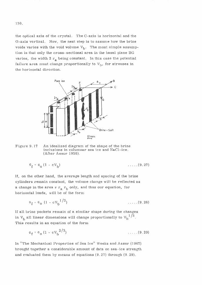
130.
the optical axis of the crystal. The C- axis is horizontal and the
G-axis vertical. Now, the next step is to assume how the brine
voids varies with the void volume Vb' The most simple assump
tion is that only the cross- sectional area in the basal plane BG
varies, the width 2 r a being constant. In this case the potential
failure area must change proportionally to Vb, for stresses in
the horizontal direction.
Figure 9.17
Pure ice F
B
An idealized diagram of the shape of the brine inclusions in columnar sea ice and NaCl-ice. (After Assur 1958).
. .... (9.27)
If, on the other hand, the average length and spacing of the brine
cylinders remain constant, the volume change will be reflected as
a change in the area 7f r a rb only, and thus our equation, for
horizontal loads, will be of the form
..... (9.28)
If all brine pockets remain of a similar shape during the changes
in Vb all linear dimensions will change proportionally to Vb 1/3.
This results in an equation of the form
..... (9.29)
In liThe Mechanical Properties of Sea Ice" Weeks and Assur (1967)
brought together a considerable amount of data on sea- ice strength
and evaluated them by means of equations (9.27) through (9.29).

The best fit was mostly obtained with equation (9.28). See for
example figure 9. 16 for NaCl- ice.
131.
The most extensive research have been done with ring tensile
tests. Experiments by Graystone, Langleben, Dykins, Pounder
and Frankenstein (cited by Weeks and Assur 1967) give values
on 00
ranging between 2. 65 MPa and 2. 96 MPa and on c of equa
tion (9.28) between 1.31 and 2.07 for Vb < 0.63. For 0.63 < Vb<
0.8 the failure is approximately constant of = O. 67 MPa
which might be explained the hypothesis that there
still must exist some skeleton of ice even at this high content of
brine.
In connection with thermal ice pressure we are mostly concerned
with stress in horizontal directions, that is parallel to the plane
BC of figure 9. 17. Unfortunately, published results from such
compression tests have not been evaluated in terms of the sea
ice model described in this paragraph. However, Butkovich
(Weeks and Assur 1967) found median strength values ranging
from 7.8 MPa at - 50 C to 12 MPa at - 16 0 C for stress applied
vertically, that is along the G-axis. Average values for horizon
tal stress in the same temperature interval vary from 2. 1 to
4.3 MPa. Unfortunately, the salinity or void volume of the cores
is unknown. The ring tensile tests seem to be unsensitive to the
orientation of the specimens, while tensile and compressive tests
show that horizontal loads give strength values approxiamtely 1/3
of those received from tests with vertical loads. (J ohnson 1972).
9.72
It should be possible to extend the use of the structural model of
sea-ice described in the previous paragraph to calculating elas
ticity.
For stress in the vertical direction (G-axis) the following relations
will approximately hold for the deformation, again assuming the
voids to be full of brine and neglecting the interruptions of the
vertical oblong voids. See figures 9. 17 and 9. 18.
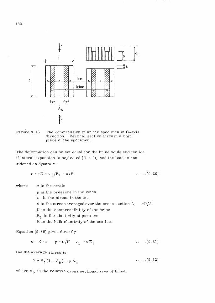
132.
J L
£
Figure 9.18 The compression of an ice specimen in G-axis direction. Vertical section through a unit piece of the specimen.
The deformation can be set equal for the brine voids and the ice
if lateral expansion is neglected (V = 0), and the load is con
sidered as dynamic.
where E is the strain
p is the pressure in the voids
G 1 is the stress in the ice
G is the stress averaged over the cross section A,
K is the compressibility of the brine
El is the elasticity of pure ice
E is the bulk elasticity of the sea ice.
Equation (9. 30) gives directly
G = E . E
and the average stress is
where Ab is the relative cross sectional area of brine.
.. ... (9.30)
=P/A
..... (9. 31)
..... (9.32)

The combination of equations (9.30) to (9.32) yields the bulk
elasticity modulus
133.
E El + (1/K - ..... (9.33)
or if Vb = Ab is inserted
E = ..... (9.34)
The modulus of elasticity in the vertical direction is thus hypotheti
cally a linear function of the brine volume. By equation (9.34) the
elasticity modulus as a function of temperature and ice salinity can
be obtained, calculating the brine volume from equation (2. ] 0) or
(2.12), the ice elasticity from equation (9.7) or (9.8), and assuming
a value on the compressibility of the brine.
.. ... (9.35)
K is a value for air free water at 50 C and normal pressure. Of
course, it had been desireable to have a value for brine in the
relevant temperature range.
Equation (9.34) should also hold for a random distribution of brine
voids since the relative brine area Ab in any cross section equals
the brine volume Vb'
If one considers the horizontal deformation in a sea-ice cover, however,
a more complicated model should be built. For this purpose the dia
gram of figure 9. 17 is simplified further by substituting the brine
voids by rectangular tubes with the horizontal cross- sectional area
la . lb' See figure 9. 19. B
A""""'~~,,£------,*""-~C
Figure 9.19 A further simplification of the diagram of sea ice for the purpose of calculating its modulus of elasticity.
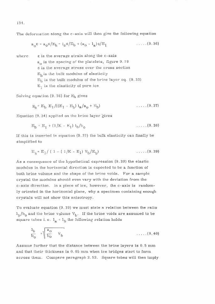
134.
The deformation along the c-axis will then give the following equation
· .... (9.36)
where E is the average strain along the c-axis
is the of the figure 9. 1 9
Cl is the average stress over the cross section
is the bulk modulus of
is the bulk modulus of the brine eq. (9.33)
is the of pure ice
(9.36) for
· .. , , (9. 37)
Equation (9. on the brine layer
+ (1 /K El) ..... (9.38)
If this is inserted in equation (9.37) the bulk elasticity can finally be
.LU.ljJ.L.Li.l.C;U to
E = h · .... (9.39)
As a consequence of the hypothetical expression (9.39) the elastic
rnodulus in the horizontal direction is expected to be a function of
both brine volume and the shape of the brine voids. For a sample
crystal the modulus should even vary with the deviation from the
c-axis direction. In a piece of ice, however, the c-axis is random-
oriented in the horiz.ontal plane, why a specimen containing enough
will not show this rl.III,.,' ... ,
To evaluate equation (9. 39) we must state a relation between the ratio
lb/bo and the brine volume . If the brine voids are assumed to be
square tubes i. e. la = lb the following relation holds
· , ... (9.40)
Assume further that the distance between the brine layers is O. 5 mm
and that their thicknes s is O. 05 mm when ice bridges start to form
across them. paragraph 2. 52. Square tubes will then imply
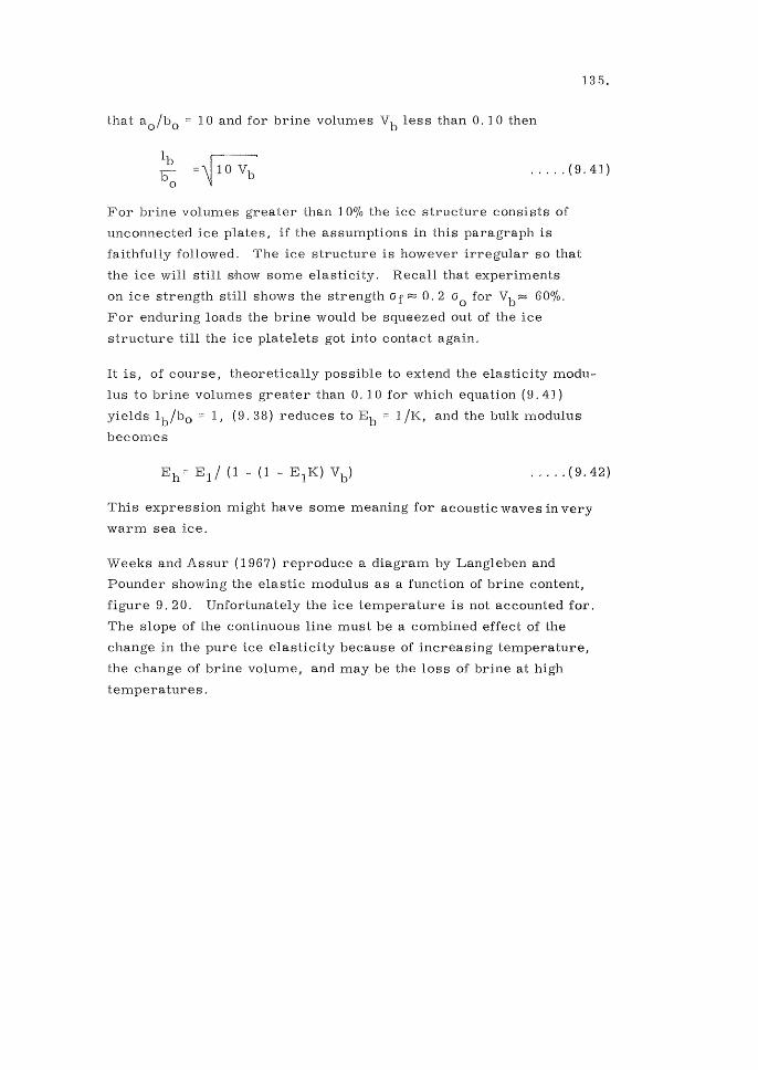
135.
that ao/bo = 10 and for brine volumes Vb less than O. ] 0 then
..... (9.41)
For brine volumes greater than 10% the ice structure consists of
unconnected ice plates, if the assumptions in this paragraph is
faithfully followed. The ice structure is however irregular so that
the ice will still show some elasticity. Recall that experiments
on ice strength still shows the strengthGf:=::: 0.2 Go for Vb~ 60%.
For enduring loads the brine would be squeezed out of the ice
structure till the ice platelets got into contact again.
It is, of course, theoretically possible to extend the elasticity modu
lus to brine volumes greater than 0.10 for which equation (9.4])
yields lb/bo = 1, (9. 38) reduces to Eb = l/K, and the bulk modulus
becomes
..... (9.42)
This expression might have some meaning for acoustic waves in very
warm sea ice.
Weeks and Assur (1967) reproduce a diagram by Langleben and
Pounder showing the elastic modulus as a function of brine content,
figure 9.20. Unfortunately the ice temperature is not accounted for.
The slope of the continuous line must be a combined effect of the
change in the pure ice elasticity because of increasing temperature,
the change of brine volume, and may be the loss of brine at high
temperatures.
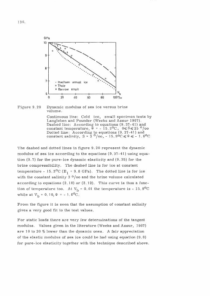
136.
Figure 9.20
GPa 10 ~~--~----~----~----~----~
9
8
7 Isachsen annual ice o Thule f:, Barrow strait
6L-____ ~ __ --+-----+_----+_--~Vb o 20 40 60 80 100"/00
Dynamic modulus of sea ice versus brine volume.
Continuous line: Cold ice, small specimen tests by Langleben and Pounder (Weeks and Assur 1967). Dashed line: According to equations (9.37-41) and constant temperature, 9 = - 15. 30C, O~ S~ 25 0/00 Dotted line: According to equations (9. 37 -41) and constant salinity, S = 3 0/00, - 15. 90C~ Q ~ - 1. 60C
The dashed and dotted lines in figure 9.20 represent the dynamic
modulus of sea ice according to the equations (9.37-41) using equa
tion (9.7) for the pure-ice dynamic elasticity and (9.35) for the
brine compressibility. The dashed line is for ice at constant
temperature - 15. 30C (El = 9.8 GPa). The dotted line is for ice
with the constant salinity 3 0/00 and the brine volume calculated
according to equations (2.10) or (2.12). This curve is thus a func
tion of temperature too. At Vb = 0.01 the temperature is - 15. 90C
w hil eat Vb = O. 1 0> Q l. 60 C .
From the figure it is seen that the assumption of constant salinity
gives a very good fit to the test values.
For static loads there are very few determinations of the tangent
modulus. Values given in the literature (Weeks and Assur, 1967)
are 10 to 20 % lower than the dynamic ones. A fair appreciation
of the elastic modulus of sea ice could be had using equation (9.8)
for pure- ice elasticity together with the technique described above.
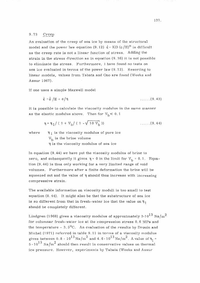
137.
An evaluation of the creep of sea ice by means of the structural
model and the power law equation (9.12) E = KD (0 /E)n is difficult
as the creep rate is not a linear function of stress. Adding the
strain in the stress direction as in equation (9. 36) it is not possible
to eliminate the stress. Furthermore, I have found no tests on
sea ice evaluated in terms of the power law (9. 12). Resorting to
linear models, values from Tabata and Ono are found (Weeks and
Assur 1967).
If one uses a simple Maxwell model
E 6/E+0/1l ..... (9. 43)
it is possible to calculate the viscosity modulus in the same manner
as the elastic modulus above. Then for Vb < 0.1
where 1] 1 is the viscosity modulus of pure ice
Vb is the brine volume
1] is the viscosity modulus of sea ice
..... (9. 44)
In equation (9.44) we have put the viscosity modulus of brine to
zero, and subsequently it gives 1] = 0 in the limit for Vb = 0.1. Equa
tion (9.44) is thus only working for a very limited range of void
volumes. Furthermore after a finite deformation the brine will be
squeezed out and the value of 11 should thus increase with increasing
compressive strain.
The available information on viscosity moduli is too small to test
equation (8.44). It might also be that the substructure of sea ice
is so different from that in fresh-water ice that the value on 111
should be completely different.
Lindgren (1968) gives a viscosity modulus of approximately 3.] 013 Ns/m2
for columnar fresh-water ice at the compression stress 0.6 lVIPa and
the temperature - 3. 5 °C. An evaluation of the results by Drouin and
Michel (1971) referred in table 9.11 in terms of a viscosity modulus . 13 2 13 2
gIves between 0.8 . 10 Ns/m and 4.6· 10 Ns/m. A value of 111
5.1013 Ns/m2 should then result in conservative values on thermal
ice pressure. However, experiments by Tabata (Weeks and Assur
138.
1967) show that sea ice with the salinity 4. 9 0100 and temperature
- 1. 90 C has a horizontal modulus of viscosity of I] ::::: 7·1 012Ns 1m2 .
For this combination of salinity and temperature equation (9.44)
gives 1] = 0 since Vb> 0.10 according to figure 2.20.
0.10 valume J Vb
(7· ro'2/0.13) -- .... X-
0.15
9.21 The viscosity modulus of sea ice as a function of brine volume Vh :rccording to equation (9.44) and with 1]1 = 5 . ID Ns hT2 . For Vb> 10% the constant value I] = 7 . 101 Ns/m 2 is recommended.
In figure 9.21 above the function (9.44) is illustrated with 1)1 =
5 . 1013 Ns 1m2 and the value by Tabata on 1) = 7 . 1012 Ns 1m2 and
Vb ~ O. 13. It is recommended to use the dashed 'curve for pressure
calculations or 1) = 5 . 10 13 .
9.74 Model of Sea Ice -'='-----------------
For the purpose of calculating ice pressure in columnar sea ice a
simple Maxwell model will be used with a spring in series with a
dashpot. Its deformation is described by the simple equation
where
E: = 6 IEh + G 11] Et is the bulk elastic modulus, eq. (9.39)
1) is the bulk viscosity modulus, fig. 9.20
G is the stress
E. is the strain rate
..... (9.45)
As has been described in the preceeding paragraphs the bulk moduli
are, however, very difficult to evaluate. Furthermore, the whole
139.
process of thermal expansion and brine volume variations with
temperature is a complex matter to calculate, even if the elements
described in paragraphs 2.53, 3.4 and 6.2 are fairly well verified.
Each conclusion relies on many simplifying assumptions, why they
taken together indicate that there is little to benefit from constructing
a more complex model than (9.45) for the purpose of calculating
thermal ice pressure. For the purpose of calculating the bearing
capacity of ice covers, ice loads against structures, or ice breaking
forces it may be of use to apply a more complex model. See for
example Weeks and Assur (1967).
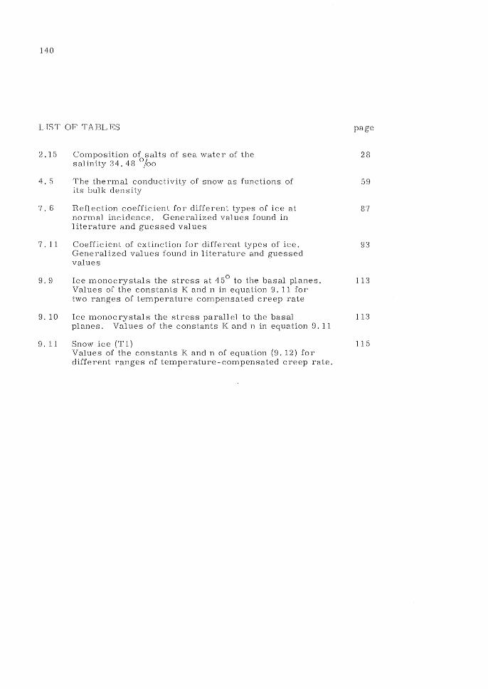
140
LIST OF TABLES
2.15
4.5
7 . 6
7 . 11
9.9
9. 10
9. 11
Composition of salts of sea water of the salinity 34.48 0/00
The thermal conductivity of snow as functions of its bulk density
Reflection coefficient for different types of ice at normal incidence. Generalized values found in literature and guessed values
Coefficient of extinction for different types of ice. Generalized values found in literature and guessed values
Ice monocrystals the stress at 45 0 to the basal planes. Values of the constants K and n in equation 9. 11 for two ranges of temperature compensated creep rate
Ice monocrystals the stress parallel to the basal planes. Values of the constants K and n in equation 9.11
Snow ice (T 1) Values of the constants K and n of equation (9.12) for different ranges of temperature-compensated creep rate.
page
28
59
87
93
113
113
115
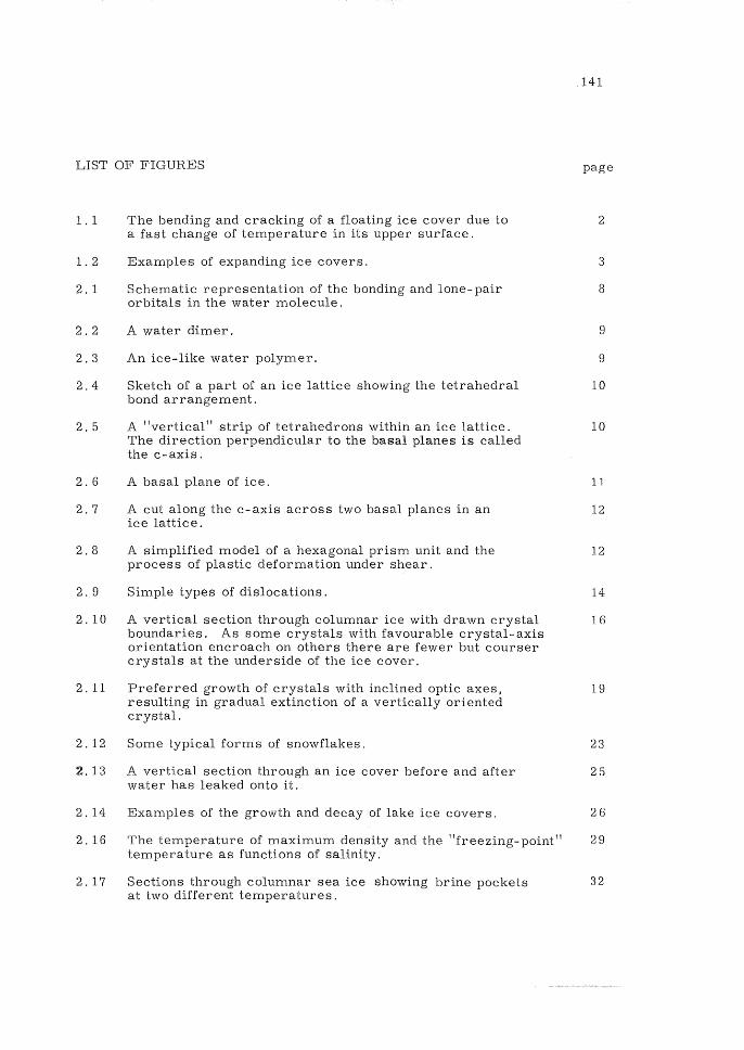
141
LIST OF FIGURES page
1. 1 The bending and cracking of a floating ice cover due to 2 a fast change of temperature in its upper surface.
1. 2 Examples of expanding ice covers. 3
2.1 Schematic representation of the bonding and lone-pair 8 orbitals in the water molecule.
2.2 A water dimer. 9
2.3 An ice-like water polymer. 9
2.4 Sketch of a part of an ice lattice showing the tetrahedral 10 bond arrangement.
2.5 A llvertical" strip of tetrahedrons within an ice lattice. 10 The direction perpendicular to the basal planes is called the c-axis.
2.6 A basal plane of ice. 11
2.7 A cut along the c-axis across two basal planes in an 12 ice lattice.
2.8 A simplified model of a hexagonal prism unit and the 12 process of plastic deformation under shear.
2. 9 Simple types of dislocations. 14
2. 10 A vertical section through columnar ice with drawn crystal 16 boundaries. As some crystals with favourable crystal-axis orientation encroach on others there are fewer but courser crystals at the underside of the ice cover.
2. 11 Preferred growth of crystals with inclined optic axes, 19 resulting in gradual extinction of a vertically oriented crystal.
2.12 Some typical forms of snowflakes. 23
2. 13 A vertical section through an ice cover before and after 25 water has leaked onto it.
2.14 Examples of the growth and decay of lake ice covers. 26
2.16 The temperature of maximum density and the llfreezing_point 11 29 temperature as functions of salinity.
2. 17 Sections through columnar sea ice showing brine pockets 32 at two different temperatures.

142.
2.18
2.19
2.20
2.21
3.1
3.2
3.3
3.4
3.5
3.6
3.7
4.1
4.2
4.3
4.4
4.6
4.7
5.1
"Freezing-point curve" of sea-water brine showing the concentration of brine in equilibrium with ice versus temperature. The various solid salts are listed opposite the segment of the curve in which they are the dominant salt crystallizing.
Brine migration along the temperature gradient.
Phase relations, by volume, of sea ice of four typical salinities.
An idealized diagram of the shape of the brine inclusions in columnar sea ice and NaCl ice.
Compact density as a function of temperature for freshwater ice.
The density of the snow cover in the winter of 1915/16, at Gasbornshyttan and Gimo.
Mean course of density of snow cover in the winters of 1909/10 - 1917/18.
A comparison of the density of columnar sea ice with the salinity 20 0/00 as a function of temperature according to the relations in this chapter, and according to Anderson (1960) and Schwerdtfeger (1963).
The density of columnar sea ice without air inclusions as a function of temperature for different salinities.
Plots of density and of salinity as a function of depth. Annual sea ice in Hudson Bay near Churchill, Manitoba.
Coefficient of volume expansion versus temperature for three salinities for void free sea ice.
Thermal conductivity of ice as a function of temperature according to different authors.
The conductivity of porous fresh-water ice as a function of air content at OOC.
Models of columnar sea ice to be used for calculating thermal conductivity in the vertical direction.
The bulk conductivity of columnar sea ice as a function of temperature for different salinities and air contents.
The thermal conductivity of snow as functions of its bulk density.
The "relative" conductivity of Anisimov in per cent.
The specific heat capacity of sea ice as a function of salinity and temperature.
34
36
36
39
42
45
45
48
49
50
51
53
54
55
57
60
61
65

143.
5.2 The deficit of heat (negative entalpity) of sea ice 67 relative to its freezing poip..t as a function of tempera-ture for the salinities 3 and 20 0/00.
6.1 The temperature diffusivity of fresh-water ice as a 70 function of temperature.
6 2 The temperature diffusivity of porous fresh-water 71 ice as a function of its air content at oOe.
6. 3 The temperature diffusivity of columnar sea ice in 72 the vertical direction as functions of temperature for the salinities O. 3 and 20 0/00.
6.4 The temperature diffusivity of snow as a function of 73 its bulk density according to the relations for thermal conductivity of Abel, Bracht and Deveaux.
7. 1 Spectra for solar and sky radiation at clear sky. 78 Black- body ra.diation for 6000K and 270K.
7. 2 Refraction of light. 80
7. 3 The spherical a.nd ellipsoidal vector surf~ces for an 81 optically uniaxial and positive crystal. The difference between the surfaces is exaggerated.
7.4 The reflectio~ coefficient of a polished flawless ice 84 surface at -3 e and A 0.5 pm.
7 . 5 Field measurements of reflection coefficient of snow. 86
7.7 Reflexion, refra.ction, scattering, and transmission 88 of a beam of light in an ice cover.
7.8 Spectral curves of the ratio of transmitted light for 89 samples of ice 2 cm thick.
7. 9 Infrared absorption spectrum of ice in the range 90 1 . 4 pm ~ A ~ 4 pm.
7.10 Summary of results from Mellor'" s (1965) attenuation 91 experiments.
8.1 Radiation fluxes on Feb. 28, 1962, clear day. Measured 96 by Schwerdtfeger and Pounder (1963) on the ice of Hudson Bay (58 0 49'" N, 94 0 14'" W).
8.2 Temperatures in ice covers free from snow. 98
8.3 The temperature in a 0.10 m thick ice cover. 99
9. 1 Dependence of properties of ice on its structure. 100
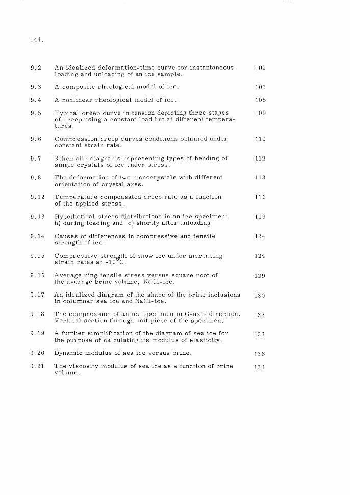
144.
9.2 An idealized deformation-time curve for instantaneous 102 loading and unloading of an ice sample.
9. 3 A composite rheological model of ice. 103
9.4 A nonlinear rheological model of ice. 105
9. 5 Typical creep curve in tension depicting three stages 109 of creep using a constant load but at different tempera-tures.
9.6 Compression creep curves conditions obtained under 110 constant strain rate.
9.7 Schematic diagrams representing types of bending of 112 single crystals of ice under stress.
9.8 The deformation of two monocrystals with different 113 orientation of crystal axes.
9. 12 Temperature compensated creep rate as a function 116 of the applied stress.
g. 13 Hypothetical stress distributions in an ice specimen: 119 b) during loading and c) shortly after unloading.
9.14 Causes of differences in compressive and tensile 124 strength of ice.
9.15 Compressive stren&.th of snow ice under increasing 124 strain rates at -10 C.
9.16 Average ring tensile stress versus square root of 129 the average brine volume, NaCl-ice.
9. 17 An idealized diagram of the shape of the brine inclusions 130 in columnar sea ice and NaCl- ice.
9.18 The compression of an ice specimen in G-axis direction. 132 Vertical section through unit piece of the specimen.
9. 19 A further simplification of the diagram of sea ice for 133 the purpose of calculating its modulus of elasticity.
9.20 Dynamic modulus of sea ice versus brine. 136
9.21 The viscosity modulus of sea ice as a function of brine 138 volume.
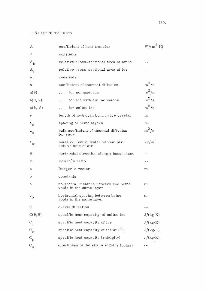
145.
LIST OF NOTATIONS
A
A
Ab
A. 1
a
a
a(8)
a( 8, v)
a(8, S)
a
a 0
a s
a w
B
B
b
b
b
b 0
e
e(8, S)
e. 1
e 0
e p
e s
coefficient of heat transfer
constants
relative cross- sectional area of brine
relati ve cross sectional area of ice
constants
coefficient of thermal diffusion
for compact ice
for ice with air inclusions
for saline ice
length of hydrogen bond in ice crystal
spacing of brine layers
bulk coefficient of thermal diffusion for snow
mass content of water vapour per unit volume of air
horizontal direction along a basal plane
Bowen'" s ratio
Bur ger" s vector
constants
2 W/(m ·K)
m2 /s
m2/s
m2 /s
m2/s
m
m
2 m /s
3 kg/m
m
horizontal distance between two brine m voids in the same layer
horizontal spacing between brine m voids in the same layer
c-axis direction
specific heat capacity of saline ice
specific heat capacity of ice
specific heat capacity of ice at aOe
specific heat capacity (entalpity)
cloudiness of the sky in eighths (octas)
J /(kg-K)
J /(kg-K)
J /(kg.K)
J /(kg.K)
146.
c w
c, cl' c 2
c
c e
c 0
cl' c 2
D
D 0
d
d
d
d cr
E
Eb
Eb
E c
Eh
Et
El
E2
e a
F
F g
f(u)
f( G)
G
g
specific heat capacity of water
constants
velocity of ordinary wave
velocity of extraordinary wave
speed of light in empty space
speed of light in different materials
coefficient of diffusion of gas or the molecules in ice
constant
differential operator
constants
sample diameter
crystal size, grain diameter
modulus of elasticity, static modulus of elasticity, bulk elasticity of saline ice
elastic modulus in bending
elastic modulus of brine layer
elastic modulus in compression
bulk modulus of sea ice for horizontal deformation
elastic modulus in tension
dynamic elasticity of pure ice
modulus of delayed elasticity
humidity, water vapour pressure
horizontal cross-sectional area of a brine void
vertical cross- sectional area of a brine void
wind- speed function
creep function
vertical direction
vertical length of brine voids
J /(kgoK)
m/s
m/s
m/s
m/s
m2 /s
2 m /s
m
m
Pa
Pa
Pa
Pa
Pa
Pa
Pa
Pa
Pa 2
m
2 m
m/s
-1 s
m

go
h
J
J(t)
J 0
J z
J A
K
K
K
k
L
L. 1
LS
I a
lb
mb
m bo
m. 1
m. 10
m p
n
n, nI' n 2
n e
n 0
vertical spacing between brine voids
thickness of ice cover
irradiation flux, solar irradiation
creep compliance
intensity of refracted radiation at z=Q
intensity of radiation at depth z
emitted effect per unit area and unit band-width at wave length A
coefficient for viscous deformation
11
compressibility of brine
absorption coefficient
specific latent heat of sublimation
specific latent heat of fusion of water
released latent heat of formation of a unit mass of sea ice
side of rectangular brine void section in C-direction
side of rectangular brine void section in B-direction
mass of brine to mass of system
mass ratio of brine at closure of brine voids
mass of ice (H20) to mass of system
mass ratio of ice at closure of brine voids
mass of precipitated salts to mass of system
exponent for viscous deformation
refractive indices
refractive index for extraordinary wave
refractive index for the ordinary wave
m
m
W/m2
Pa- l
W/m2
W/m2
W/m2
-2 m
-2 m Pa
Pa- 1
-1 m
J/kg
J/kg
J/kg
m
m
-n

148.
n o
P
p
p
p
Q
q
r
s
s
s
original number of dislocations per unit area
load, force
mass of precipitated salt divided by mass of solvent
pressure parameter, pressure in brine voids
effect source per unit volume
heat deficit per unit mass (ental pity)
activation energy for creep
activation energy for self diffusion
mass rate of sublimation per unit volume
heat flow per unit area
intensity of long-wave back radiation
convective (sensible) heat flux
rate of heat per unit area used for evaporation
intensity of incoming long-wave radiation
rate of heat per unit area used to melting
net incoming short-wave radiation flux
rate of change of stored heat per unit area due to change of temperature
reflexion coefficient, albedo
characteristic radius of brine void
characteristic radius of brine void
the universal gas constant
salinity, mass of salt to mass of solution
cross- sectional area of specimen
salinity of ambient sea water
salinity of brine
salt ratio, mass of salt in solution to mass of solvent
-2 m
N
Pa
W/m3
J/kg
J/mol
J/mol
kg/(s m3
)
W/m2
W/m2
W/m2
W/m2
W/m2
W/m2
W/m2
W/m2
m
m
J /( mol·K)
sb salt ratio of brine
T, T l' T 2' T 3 absolute temperature
T a absolute temperature of air
time coordinate, point of time
u
v
x
Y(t)
z
C£
C£
y
y
y
E
E
E (t)
wind speed
volume fraction of brine
volume fraction of brine for which the sea-ice strength is nil
volume fraction of ice
coordinate
relaxation modulus
depth in ice or snow cover
angle of incidence
linear coefficient of thermal expansion
constants
coefficient for the mass of hydrated water
angle of refraction
rate of increase of dislocations
volume coefficient of thermal expansion
psycrometric constant
surface energy
difference operator
emissivity
strain, deformation per unit length
emissivity of the atmosphere (air)
deformation as a function of time
diverse amounts of deformation
viscosity modulus of sea ice
viscosity modulus
149.
K
K
s
m/s
m
Pa
m
rad, degrees
K- 1
rad, degrees
-2 m
Pa/K
J/m2
2 Ns/m
2 Ns/m
150.
112
8
8 a
8.r .1
8 rn
"A.
A. (8)
"A (Q, S)
"A (e, v)
"A (Q,\},S)
p
p (8)
p(e,S)
p(e, v )
p(Q,S,\})
viscosity modulus
temperature
air temperature
freezing point
melting point
specific thermal conductivity
wave-length
conductivity of pure ice
conductivity of saline ice with air inclusions
conductivity of fresh-water ice with air inclusions
conducti vity of saline ice with air inclusions
"A ( OOe) conductivity of ice at OOC.
thermal conductivity of air
thermal conductivity of brine
wave-length for maximum intensity of radiation
imaginary part of the complex refractive index, extinction coefficient
contents of air voids by volume
Poisson~ s modulus
integration variable
density
compact density of ice
bulk density of saline ice without air inclusions
bulk density of fresh-water ice
bulk density of saline ice with air inclusions
density of brine at equilibrium temperature
W/(moK)
m
W /(m·K)
W/(m·K)
W/(moK)
W /(moK)
W /(m·K)
W/(m.K)
W /(moK)
m
3 kg/m
kg/m3
kg/m3
kg/m3
kg/m3
3 kg/m
o
o
o (t)
°c
o max
o t
o 0
0 0
o 1
compact density of ice
density of precipitated salts
bulk density of snow
compact density of water
compact density of ice at oOe
stress
Stefan-Boltzmann" s constant
stress as a function of time
compressive strength
strength of sea ice
maximum yield strength of ice
tensile strength
strength of fictitious brine-free sea ice
stress value
stress in the ice phase
integration help variable
stress constant
plane porosity
differential operator
= '0/ Clt first derivative with respect to time
= l/ a t 2 second derivative with respect to time
3 kg/m
3 kg/m
3 kg/m
3 kg/m
3 kg/m
Pa
Pa
Pa
Pa
Pa
Pa
Pa
Pa
s
Pa
-1 s
-2 s
151.

152.
REFERENCES
Ager, B. H :son, (1960): Studier over isforhallandena i Norrland, Dalarna och Varmland, Virkesavlaggning pa is. Statens Skogsforskningsinstitut, Avdelningen fOr arbetslara. Rapporter 1960 Nr 10. (Studies of the ice conditions in northern Dalecarlia and Varmland. The storing of timber on ice covers).
Ager, B. H:son. (1963 a): Preparering av virkesavlagg pa is. Skogshogskolan, Stockholm. 1963. (Preparing places for the storage of timber on ice covers).
Ager, B. H:son. (1963 b): Studies of the Density of Naturally and Artificially Formed Fresh-Water Ice. Journal of Glaciology, Vol. 1963, No. 32.
Anderson, D. L. (1960): The physical constants of sea ice. Research applied in industry. Vol. XIII, No. 8, London 1960.
Anisimov, M. 1. (1961): Approximativ vardering ay formler fOr snons varmeledningsformaga. Meteorologija i gidrologija, No. 9, Moskva 1961. (An approximate evaluation of formulae for the thermal conductivity of snow. Translated into Swedish by SMHI).
Armstrong, T., Roberts, B. and Swithinbank, C. (1966):Illustrated Glossary of Snow and Ice. Scott Polar Research Institute, Special publication, Number 4, University Printing House, Cambridge 1966.
Assur, A.: (1958): Composition of Sea Ice and its Tensile Strength. National Academy of Sciences, National Research Council, Publ. 598, "Arctic Sea Ice" J USA 1958.
Bader, H.l;l.nd Kuroiwa, D. (1962): The Physics and Mechanics of Snow as a Material, CRREL, Cold Regions Science and Engineering II-B.
The Baltic Ice Code (1959): Ostersjokoden for isunderrattelser. SMID, Meddelanden, Serie E, nr 10, P. A. Norstedt och Saner, Stockholm 1959.
Bengtsson, L. (1976): Snowmelt Estimated from Energy Budget Studies. Nordic Hydrology, 7, 1976, pp 3-18.
Bennington, K. O. (1963): Some Crystal Growth Features of Sea Ice. Journal of Glaciology, Vol. 4, 1963, No. 36.
Bergdahl, L. (1978): Thermal Ice Pressure in Lake Ice Covers. Department of Hydraulics, Chalmers University of Technology, Report Series A:2.
Bergdahl, L. and Wernersson, L. (1977): Calculated and Expected Thermal Ice Pressures in Five Swedish Lakes. Department of Hydraulics, Chalmers University of Technology! Report Series B:7.
Bergen, J. D. (1975): A Possible Relation of Albedo to the Density and Grain Size of Natural Snow Cover. Water Resources Research, Vol. 11, No 5, Oct. 1975.
153.
Brill, R. (1957): Structure of Ice. Snow Ice and Permafrost Research Establishment. Report No 33, July 1957.
Brunt, D. (1944): Physical and dynamical meteorology. Cambridge 1944.
Butiagin, I. P. (1966): Hallfasthet hos is och istacke (naturundersokningar fran Sibiriens floder). Sibiriska forskningsinstitutet fOr energetik. Novosibirsk 1966. (Strength of ice and ice cover, field studies from the rivers of Sibiria. Sibirian research institute for ener getics. Translated into Swedish by SMHI, 1969).
Butkovich, T. R. (1954): Ultimate Strength of Ice. SIPRE Res. Rep.] 1, 1954.
Butkovich, T. R. (1955): Density of Single Crystals of Ice from a Temperate Glacier. Journal of Glaciology, Vol. 2, p 553,1955.
Butkovich, T. R. (1957): Linear Thermal Expansion of Ice. SIPRE Research Report 40 (1957), US Army, vVilmette, Illinois.
Carter, D. (1970): Brittle Fracture of Snow Ice, IAHR Ice Symposium, Reykjavik 1970.
Carter, D. (1972): Brittle Fracture of Polycrystalline Ice under Compressive Loadings. IAHR Ice and Its Action on Hydraulic Structures, Leningrad 1972.
Cherepanov, N. V. and Kamyashnikova, A. V. (1971): Sizes and Shapes of Congealed Ice Crystals. In Yakovlev 1971, pp 170.
Cox, G.F.N. and vVeeks, 'IV. (1973): Salinity Variations in Sea Ice, Research Report 310, CRREL, Hannover, New Hampshire, 1973.
Dietrich, G. and Kalle, K. (1967): General Oceanography, John Wiley and Sons Inc., New York 1967.
Dorsey, N. E. (1940): Properties of Ordinary Water-Substance, New York: Reinhold Publishing Corp. 1940.
Drouin, M. and Michel, B. (1971): Les poussees d'" origine thermique exercees par les couverts de glace sur les structures hydrauliques. Rapport S-23 Genie Civil, Universite Laval, Quebec 1971.
FlUgge, W. (1975): Viscoelasticity, Springer-Verlag, New York 1975.
Frankenstein and Garner, (1967): Linear Relationship of Brine Volume and Temperature from -0.5 -- 22. 90 C for Sea Ice. Journal of Glaciology, Vol. 6, No. 48, P 943-944.

154.
Fremling,S.(a):GrundHiggande erfarenheter om is i sjoar och ttlvar. SMHI. Stencil. Stockholm. (Fundamental experience of ice in lakes and rivers).
Fremling, S. (1968): Om istillvttxt och isbttrighet pa sjoar. Foredrag vid SFM studiedagar i Arvidsjaur 1968-03-08. SMHI, HBI. (On the growth of ice and the carrying capacity of ice covers on lakes. A lecture in Arvidsjaur, March 8, 1968).
Fremling, S. (1975): Nordic Ice Terms, Draft to Nordic IHD 1975. Continued under IHP, Stockholm.
Frolov, A.D. and Slesarenko, Y.E. (1972): Characteristics of Elasticity of Sea Ice of Different Compositions. IAHR. Ice Symposium Leningrad 1972.
Gaitskhoki, B.Y. (1970 a): Spectral Transmission of Snow and Some Ice Varieties. In Bogorodskij (1970).
Gaitskhoki, B. Y. (1970 b): A Photometric Model of the Snow-Ice Cover. In Bogorodskij (1970).
Glen, J. W. and Stephens, R. W. B. (1958): The Mechanical Properties of Ice. The Plastic Properties of Ice Advances in Physics. Vol. VII, No 25-28. London 1958.
Gold, L. W. (1958): Some Observations on the Dependence of Strain on Stress for Ice. Canadian J. of Physics, Vol. 36, No 10, Oct 1958.
Gold, L. W. (1958): Influence of Snow Cover on Heat Flow from the Ground. Some Observations Made in Ottawa Area. NRC of Canada Res. Paper No 63 of the Division of Building Research.
Gold, L. W. (1965): The Initial Creep of Columnar-Grained Ice. Canadian J. of Physics. Vol 43 1965.
Gold, L. W. (1968): Elastic and Strength Properties of Fresh-Water Ice. Ice Pressure against Structures. National Research Council (of Canada). Technical Memorandum No 92, Ottawa 1968.
Gold, L. W. (1977): Eng.ineel'ing Properties of Fresh-Water Ice. J. of Glaciology, Vol. 19, No. 8.1.
Harvey, H.W. (1966): The Chemistry and Fertility of Sea Waters, Cambridge University Press, London 1966.
Hirayama, K., Schwarz, J. and Wu, H. C. (1973): Model Technique for the Investigation of Ice Forces on Structures. 2nd International Conference on Port and Ocean Engineering under Arctic Conditions, Reykjavik 1973.
Hobbs, Peter V. (1974): Ice Physics, Clarendon Press, Oxford 1974.
Janson, L.-E. (1963): Frost Penetration in Sandy Soil. Elanders Boktryckeri AB. Goteborg 1963.
155.
Johnson, P.R. (1972): The Modulus of Elasticity of Sea Ice Shown by Direct Tension and Compression Tests of Small Specimens. IAHR Symposium Ice and its action on hydraulic structures. Leningrad 1972.
Jumppanen, P. (1973): Ice Thermal Loads against Walls of Water Reservoirs. 2nd Int. Conf. on Port and Ocean Engineering under Arctic Conditions. Reykjavik 1973.
Kalle, K.: Fluchtentafeln zur Bestimmung der Dichte aus Saltzgehalt und Temperatur des Meerwassers. Aus dem Archiv der Deutschen Seewarte etc. . . .. 60. Band Nr 2.
Kalle, K. (1943): Der Stoffhaushalt des Meeres. Probleme der Kosmischen Physik Bd 23, Leipzig 1943.
Kivisild, H. R. (1970): River and Lake Ice Terminology. IAHR. Ice Symposium, Reykjavik 1970.
Knight, C.A. (1963): Studies of Arctic Lake Ice. Journal of Glaciology, Vol. 4 1963 , No. 33.
Krausz, A. S. (1968): Plastic Deformation of Fresh- Water Ice. In "Ice Pressure against Structures ". National research council. Technical memorandum no. 92, Ottawa 1968.
Lavrov, V. V. (1969): Deformation and Strength of Ice. Arctic and Antarctic Scientific Research Institute (Leningrad 1969), Israel Program for Scientific Translations, Jerusalem 1971.
Lavrov, V. V. (1971): Scale Effect as an Indication of Ice-Breaking Mechanism. In Yakovlev 1971, pp 26.
Lazier, S. S. and Metge, M. (1972): Observations on Thermal Cracks in Lake Ice. IAHR Ice Symposium, Leningrad 1972.
Lewis, E. L. (1966): Heat Flow through Winter Ice. Conference on Low Temperature Science, Contribution, No. 62, Sapporo, Japan 1966.
Lindgren, S. (1968): Istryck vid temperaturhojningar. Institutionen fOr vattenbyggnad, KTH, Stockholm 1968. (Ice Pressure at Increases of Temperature).
Lindgren, S. (1970): Thermal Ice Pressure, IAHR Ice Symposium, Reykjavik 1970.
Liljequist, G. H. (1962): Meteorologi, Generalstabens litografiska anstalt, Stockholm.
Lyons, J.B. and Stoiber, R.E. (1959 a): Crystallographic Orientation in Lake and Artificial Ice. Dartmouth College, Hanover, New Hampshire, 1959. Scientific Report No 2, Contract AF 19 (604) 2159.
Lyons, J. B. and Stoiber, R. E. (1959 b): The Absorptivity of Ice, A Critical Review, Dartmouth College, Hanover, New Hampshire, Scientific Report No 3, Contract AF 19 (604) 2159.
15G,
Lyons, J.B. and Stoiber, R.E. (1963): Orientation Fabrics in Lake Ice. Journal of Glaciology, V01.4, 1963, No 33.
Malmgren, F. (1927): On the Properties of Sea Ice. Norwegian North Polar Expedition with the "Maud" 1918-1925. Scientific Results, Vol 1, No 5, Bergen.
Martinec, J. (1965): Snow Cover Density Changes in an Experimental Watershed. International Symposium on Scientific Aspects of Snow and Ice Avalanches. IUGG and IAHS, Davos 1965.
Mellor, M. (1964): Properties of Snow. Report IIl-Al, Part Ill: Eng., Sect. As Snow Engineering, C. R. R. E. L. 1964.
Mellor, M. (1965): Some Optical Properties of Snow. International Symposium on Scientific Aspects of Snow and Ice Avalanches, Davos 1965. IUGG and IAHS.
Mellor, M. (1977h Engineering Properties of Snow. J. of Glaciology, Vol. 19, No. 81
Michel, B. and Ramseier, R. O. (1971): Classification of River and Lake Ice Based on Its Genesis, Structure and Texture. Departement de Genie Civil, Section Mecanique des Glaces, Universite Laval, Laval Canada.
Muguruma, J. and Kikuchi, K. (1963): Lake Ice Investigations at Peter's Lake, Alaska. J. of Glaciology, Vol. 4, 1963, No 36, sid. 689-708.
Nilsson, B. (1971): Matningar av snans vertikala densitetsfOrdelning i Sverige. Nordic IHD, Report No 1, Lammi 1971. (Measurements of the Vertical Distribution of Snow Density in Sweden).
Nord, M. and Taesler, R. (1973): Snatackets densitet och massa i Sverige. Byggforskningen Rapport 21 :1973. (The Density and Weight of the Snow Cover in Sweden).
Ono, N. (1966): Specific Heat and Heat of Fusion of Sea Ice. Conference on Low Temperature Science, Contribution No 789, Sapporo, Japan 1966.
Paily, P.P., Macagno, E.O. and Kennedy, J.F. (1~74): Winter-Regime Surface Heat Loss from Heated streams. IAHR Report No 155, Institute of Hydraulic Research, University of Iowa, Iowa City, Iowa March 1974.

157.
Peyton, H. R. {1966}: Sea Ice Strength, Geophysical Institute, University of Alaska, College, Alaska 99701.
Perey and Pounder {1958}: Crystal Orientation in Ice Sheets l Canadian Journal of Physics. Vol. 36 j No 4, p 494-502.
Peschanskii, I. S. {1971}: Static Pressure of Sea Ice in Yakovlev 1971, pp 1-4.
Pounder, E. R. {1965}: The Physics of Ice. Pergamon Press 1965.
Ramseier, R. O. {1967 a}: Self-Diffusion of Tritium in Natural and Synthetic Ice Monocrystals. J. of Applied Physics, Vol. 38, No 6, USA 1 967 .
Ramseier, R. O. {1967 b}: Self-Diffusion in Ice Monocrystals, CRREL. Research Report 232, Hanover, New Hampshire 1967.
Ramseier, R. O. (1971): Mechanical Properties of Snow Ice. Proceedings the First International Conference on Port and Ocean Engineering under Arctic Conditions. NTH, Trondheim, Aug. 23-30 1971, POAC 1971.
Ramseier, R. O. and Dickins, D.F. {1972}: A New Approach to Field and Laboratory Tests of Tensile,Compressive and Flexural Strength or Polycrystalline Fresh Water Ice. IAHR Ice and its Action on Hydraulic Structures, I:eningrad 1972.
Schwarz, J. and Weeks, \V. F. (l977)~ Engineering Properties of Sea Ice. J. of Glaciology, Vol. 19, No. 81.
Schwerdtfeger, P. (1963): The Thermal Properties of Sea Ice. Journal of Glaciology, Vol. 4 1963, No. 36.
Schwerdtfeger, P. and Pounder, E.R. (1963): Energy Exchange through an Annual Sea Ice Cover. International Association of Scientific Hydrology, Pub. No 61, 109.
Seligman (1936): Snow Structures and Ski Fields, Edinburgh 1936.
Sellers, W. D. (1965): Physical Climatology.· University of Chicago Press, Chicago och London 1965.
Shumskii, A. B. (1955): Principes de Glaciologie Structurale. 1955. Translation Annales du Centre d"'Etudes et de decum Paleontologiques. 22 okt. 1957.
SMHI (1961): Oversiktligt utHhande angaende inverkan pa isfOrhallandena inom Torne- och Kalix alv av olika alternativ for vattenkraftens utbyggnad. Avgivet pa uppdrag av ovre Norrbygdens Vattendomstol. (General opinion on the influence on the ice conditions in the rivers Torne and Kalix because of different schemes for the exploitation of the water power).

158.
Sulakvelidze (1959): The Equation of Heat Conduction of Porous Media Containing Saturated Vapour, Water, and Ice. The geophysical series No 2. Izvezdia Akademii Nauk SSSR. Moscow 1959. Translated into Swedish by SMHI, Stockholm 1961.
Sweers, H. E. (1976): A Nomogram to Estimate the Heat-Exchange Coefficient at the Air-Water Interface as a Function of Wind Speed and Temperature; A critical survey of some literature. Journal of Hydrology 30: 375-401.
Tabata (1958): Studies on Mechanical Properties of Sea Ice II-V. Low Temperature Science Ser. A. Vol. 17 P 147-66. Vol. 18 p 116-48. Vol. 19 p 187-201. 1958-1960.
Thomas, C. W. (1963): On the Transfer of Visible Radiation through Sea Ice and Snow. Journal of Glaciology. Vol. 4, No 34.
Uzuner, M. S. and Kennedy, J. F. (1974): Hydraulics and Mechanics of River Ice Jams, IIHR, Report No 161, Iowa City 1974.
Weeks, W. F. (1963): Tensile Strength of NaCl Ice. Journal of Glaciology, Vol. 4 1963, No 31.
Weeks, W. och Assur, A. (1967): The Mechanical Properties of Sea Ice. US Army, Cold Regions Research and Engineering Laboratory II- C3, Hanover 1967.
Weibull, W. (1939 a): A Statistical Theory of the Strength of Materials. Ingeniorsvetenskapsakademiens handlingar Nr 151, Stockholm 1939.
Weibull, W. (1939 b): The Phenomenon of Rupture in Solids. Ingeniorsvetenskapsakademiens handlingar Nr 153. Stockholm 1939.
Williams, G. P. and Gold, L. W. (1958): Snow Density and Climate. NRC of Canada. Research Paper No. 60 of the Division of Building Research. Transactions Engineering Institute of Canada. Vol. 2 No 2, May 1958 p 91 94.
WMO (1974): International Glossary of Hydrology, First Edition, UNESCOjWMO, WMO-No. 385-1974.
WMO Sea-Ice Nomenclature (1970): Terminology, codes, and illustrated glossary. WMO - No. 259. TP. 145-1970. Secretariat of the World Meteorological Organization, Geneva, Switzerland.
Institutionen for Vattenbyggnad
CHALMERS TEKNISKA HOGSKOLA
Meddelanden
78. Cederwall, K.: Havet som recipient. Hydrodynamiska synpunkter. Foredrag vid Sv. Havsforskningsforeningens &rsmote i Stockholm, mars 1975.
79. Sellgren, A.: Hydraulisk transport av fasta material i ror.1975.
80. Andreasson, L. och Cederwall, K.: Rubbningar av grundvattenbalansen i urbana omr&den. Hydrologisk konferens, Sarpsborg, 1975.
81. Cederwall, K.: Braddning av avloppsvatten och effekten av utjamningsbassanger. "Varlden, Vattnet och vi", Elmia 1975.
82. Cederwall, K.: Gross Parameter Solutions of Jets and Plumes. ASCE HY5, May 1975.
83. Larsson, Soren och Lindquist, Per: Kalkning av forsurade sjoar. Del I: Problembeskrivning samt utvardering av kalkningen av Ostra Nedsjon. Ex.arb. 1974:5.
84. Cederwall, K. och Svensson, T.: "Sediment flusing after dredging in tidal bays". 1975.
85. Goransson, C-G. och Svensson, T.: Stromkorsmatningar. Datorprogram for utvardering inkl. korrektion for avdrift. Mars 1976.
86. Rahm, L. och Haggstrom, S.: Oskarshamns Karnkraftverk. Modellstudier avseende kylvattenspridning vid framtida utbyggnad. Maj 1976. Del I Huvudrapport. Del 11 Bilagedel.
87. Sjoberg, A.: Berakning av icke stationara flodesforlopp i reglerade vattendrag och dagvattensystem. Aug. 1976.
Slut p& Meddelande-serien.

Institutionen for Vattenbyggnad
CHALMERS TEKNISKA HOGSKOLA
Report Series A
A: 1 Bergdahl, L.: Physics of ice and snow as affects
therm~al pressure.
A:2 Bergdahl, L.: Therm al ice pressure in
lake ice covers.
Reports Series B
1977
1978
1. Bergdahl, L.: Berakning av vagkrafter. 1977.
2. Arnell, V.: Studier av amerikansk dagvattenteknik. 1977.
3. Sellgren, A.: Hydraulic Hoisting of Crushed Ores. A feasibility study and pilot-plant investigation on coarse iron ore transportation by centrifugal pumps. 1977.
4. Ringesten, B.: Energi ur havsstrommar. 1977.
5. Sjoberg, A. och Asp, Th.: Brukar-anvisning for ROUTE-S. En matematisk modell for berakning av icke-stationara floden i floder och kanaler yid strommande tillstand. 1977.
6. Annual Report 76/77.
7. Bergdahl, Loch Wernersson, L.: Calculated and Expected Thermal Ice Pressures in Fiv~ Swedish Lakes. 1977.
8. Goransson, C-G. och Svensson, T.: Drogue TrackingMeasuring Principles and Data Handling.
9. Goransson, C-G.: Mathematical Model of Sewage Discharge into confined, stratified Basins - Especially Fjords


