Report No. 20530-80

BoliviaPoverty Diagnostic 2000June 28, 2002

Poverty Reduction and Economic Management Sector UnitLatin America and the Caribbean Region

With contributions from:INE-Instituto Nacional de EstadfsticaUDAPE-Unidad de Analisis de Polfticas Econ6micas

Document of the World Bank

Pub

lic D

iscl

osur

e A

utho

rized

Pub

lic D

iscl

osur

e A

utho

rized

Pub

lic D

iscl

osur

e A

utho

rized

Pub

lic D

iscl

osur

e A

utho

rized

CURRENCY EQUIVALENTSUS$1.0 = Bolivianos 7.1

FISCAL YEARJanuary 1 - December 31

MAIN ABBREVIATIONS AND ACRONYMS

CPI Consumer Price IndexGDP Gross Domestic ProductGRB Government of the Republic of BoliviaHDI Human Development IndexHIPC Heavily Indebted Poor CountriesIADB Inter-American Development BankINE Instituto Nacional de EstadisticaIMF International Monetary FundI-PRSP Interim Poverty Reduction Strategy PaperMECOVI Mejoramiento de las Encuestas y la Medicion de las

Condiciones de Vida en America Latina y el CaribeNBI Necesidades Basicas InsatisfechasPAN Programma Nacional de Atencion a Ninos y Ninas

Menores de Seis AnosPIDI Proyecto Integral de Dessarollo InfantilPRSP Poverty Reduction Strategy PaperSIF Social Investment FundUDAPE Unidad de Andlisis de Politicas EconomicasUNDP United Nations Development ProgrammeUSAID United States Agency for International Development

Vice President: David de FerrantiCountry Director: Isabel GuerreroPREM Director: Ernesto MayPillar Leader: John NewmanSector Manager: Norman HicksTask Manager: Quentin Wodon

TABLE OF CONTENTS

EXECUTIVE SUMMARY ............................................................................. ;

CHAPTER L TREND IN POVERTY AND INEQUALITY .............................................................................. 1

A. THIS REPORT IS A CONTRIBUTION TO BOLIVIA's NATIONAL DIALOGuE II AND PRSP .............. .......................... 1

B. THERE HAS BEEN A DECREASE IN POVERTY IN THE 1990S IN LARGE CITIES ....................................................... 4

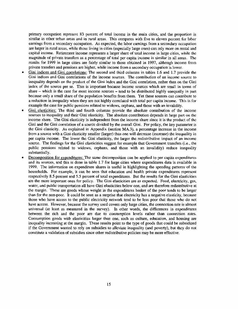
C. INEQUALITY MAY HAVE DECREASED A B IT, BUT THIS NEED NOT IMPLY A LONG TERM TREND ......... ............. 14

CHAPTER II. MICRO DETERMINANTS OF POVERTY ............................................................................. 17

A. REGRESSIONS ARE BETrER THAN PROFILES FOR ANALYZING THE DETERMINANTS OF POVERTY ......................... 17

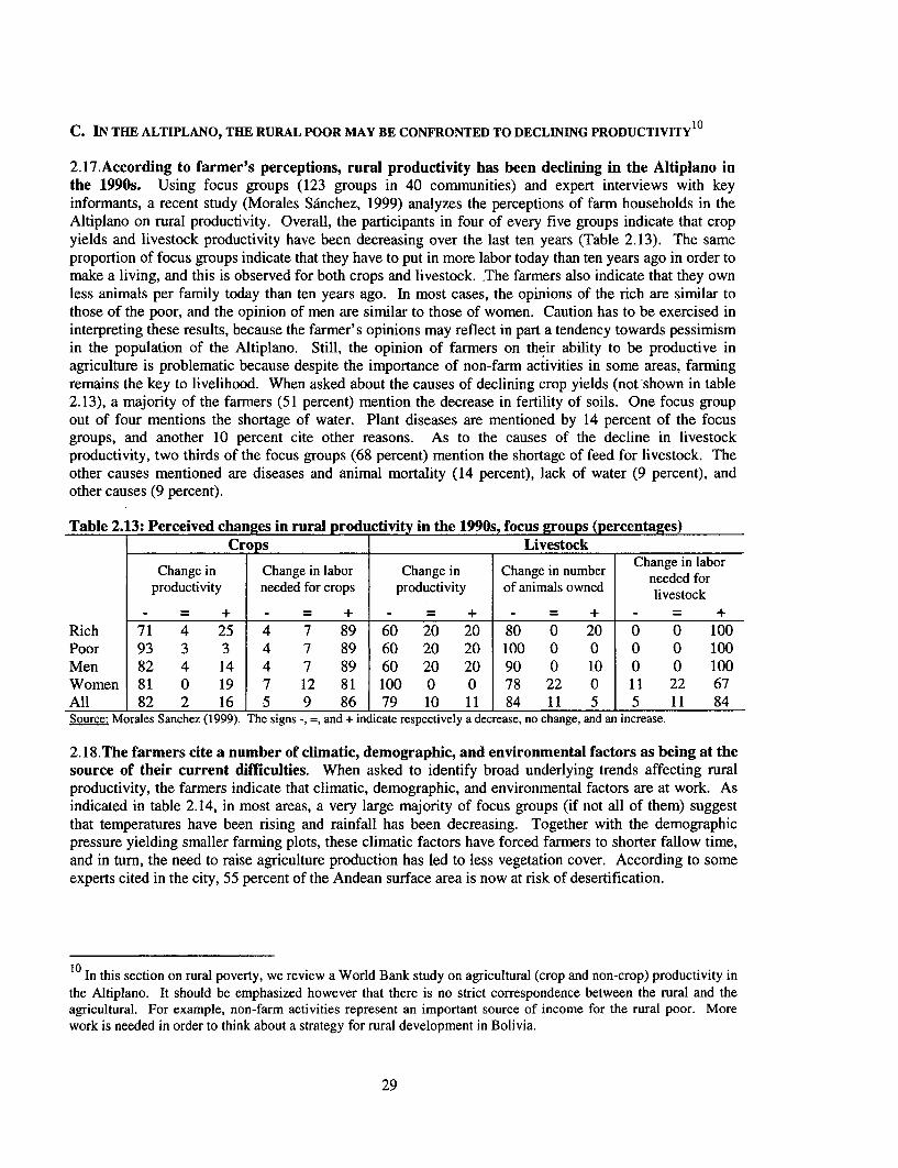
B. HOUSEHOLD STRUCTURE, EDUCATION, EMPLOYMENT, AND LOCATION ALL AFFECT POVERTY . ......................... 18C. IN THE ALTIPLANO, THE RURAL POOR MAY BE CONFRONTED TO DECLINING PRODUCTIVITY ......... ................. 29

CHAPTER HI. NON-MONETARY INDICATORS AND PRIORITIES OF THE POOR .............................. 33

A. NON-MONETARY INDICES OF WELL-BEING HAVE IMPROVED MORE THAN POVERTY ............. .......................... 33B. POVERTY CAN BE REDUCED BY ACCESS TO BASIC INFRASTRUCTURE SERVICES ................ ............................... 35C. WHILE THE POOR EMPHASIZE EMPLOYMENT, THEY ALSO VALUE OTHER BENEFITS ........................................ 44

CHAPTER IV. EDUCATION, NUTRITION AND HEALTH ............................................................................. 49

A. ENROLLMENT IN PRIMARY SCHOOL HAS IMPROVED, BUT MANY DROP OUT AND QUALITY IS Low ........ ........ 49B. INVESTMENTS IN PRE-SCHOOLS MAY HELP IN RAISING ENROLLMENT AND ACHIEVEMENT .......... .................... 53

C. THE COST OF CHILD LABOR IN TERMS OF FORGONE FUTURE EARNINGS IS SUBSTANTIAL ................................ 56

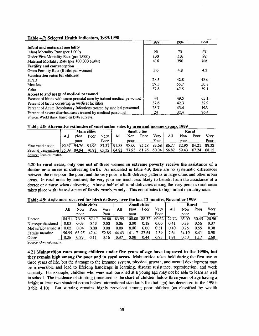
D. BOLIVIA'S PERFORMANCE IN HEALTH IS LOWER THAN IN EDUCATION ............................................................. 57

CHAPTER V. IMPACT OF GROWTH ............................................................................. 65

A. GROWTH IMPROVES BOTH MONETARY AND NON-MONETARY INDICATORS OF WELL-BEING .......... .................. 65

B. THE POOR Do NOT NECESSARILY BENEFIT EQUALLY FROM AN EXPANSION IN PUBLIC SERVICES ..................... 70

C. GROWTH ELASTICITIES OF POVERTY AND SOCIAL INDICATORS CAN BE USED FOR SIMULATIONS ......... ........... 71

REFERENCES ....... ....................................................................... 75

APPENDIX. METHODOLOGICAL ANNEXES ............................................................................. 80

MA. 1 MEASURING POVERTY, INEQUALITY AND INCOME GROWTH IN THE SURVEYS ................................................ 80MA.2 ANALYZING THE IMPACT OF VARIOUS INCOME SOURCES IN INEQUALITY ....................................................... 81MA.3 DETERMINANTS OF GROWTH, CATEGORICAL OR LINEAR REGRESSIONS ........................ ................................. 82MA.4 EDUCATION FORCE PARTICIPATION AND LABOR ...................................... ....................................... 83MA.5 WAGES AND LABOR FORCE PARTICPATION AREA VERSUS INDIVIDUAL EFFECTS .............. ............................ 84MA.6 MEASURING UNSATISFIED BASIC NEEDS IN BOLIVIA ............................................................................. 86MA.7 ESTIMATING THE COST OF CHILD LABOR IN TERMS OF FUTURE EARNINGS ................... .................................. 87MA.8 MEASURING THE IMPACT OF GROWTH ON POVERTY AND SOCIAL INDICATORS ................ .............................. 89MA.9 WHO BENEFITS FROM AN IMPROVEMENT IN ACCESS TO BASIC SERVICES? ..................................................... 90

List of Tables

Table ES. 1: Trend in Poverty and Extreme Poverty, 1993-99 ............................................................................ iiiTable ES.2: Trend in Poverty and Extreme Poverty, 1993-99 ............................................................................ iiiTable ES.3: Inequality for per capita income: Income shares, and GinilAtkinson indices, 1993-99 ........................... ivTable ES.4: Probability of Being Poor or Extremely Poor by Group, 1993-99 ........................................................... viTable ES.5: Share of the Population Poor According to Unmet Basic Needs (NBI), 2001 ......................................... xiTable ES.6: Trend in Human Development Index and Comparison with PRSP Countries, 1980-1999 ..................... xiiTable ES.7: Education Sector Indicators--Primary and Secondary Levels, 1990-97 ................................................. xviTable ES.8: Selected Health Indicators, 1989-1998 ............................................................................ xxTable ES.9: Alternative Estimates of Vaccination rates by Area and Income Group, 1999 ....................................... xxTable ES.10: Child Malnutrition by Wealth Quintile and Area, 1994 and 1998 ......................................................... xxTable ES. 11: Poverty Measures: An Hypothetical Illustration with Growth at 2 Percent Per Capita ...................... xxiii

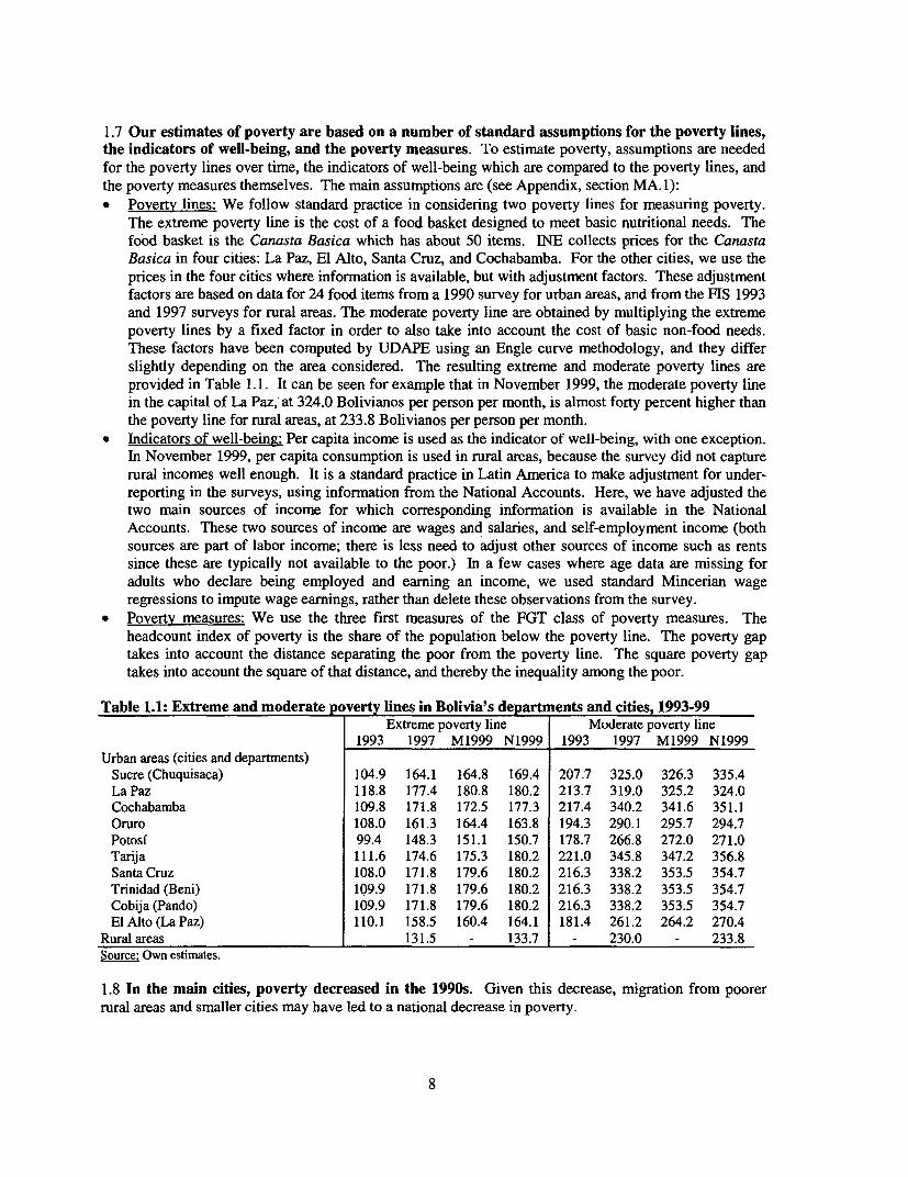
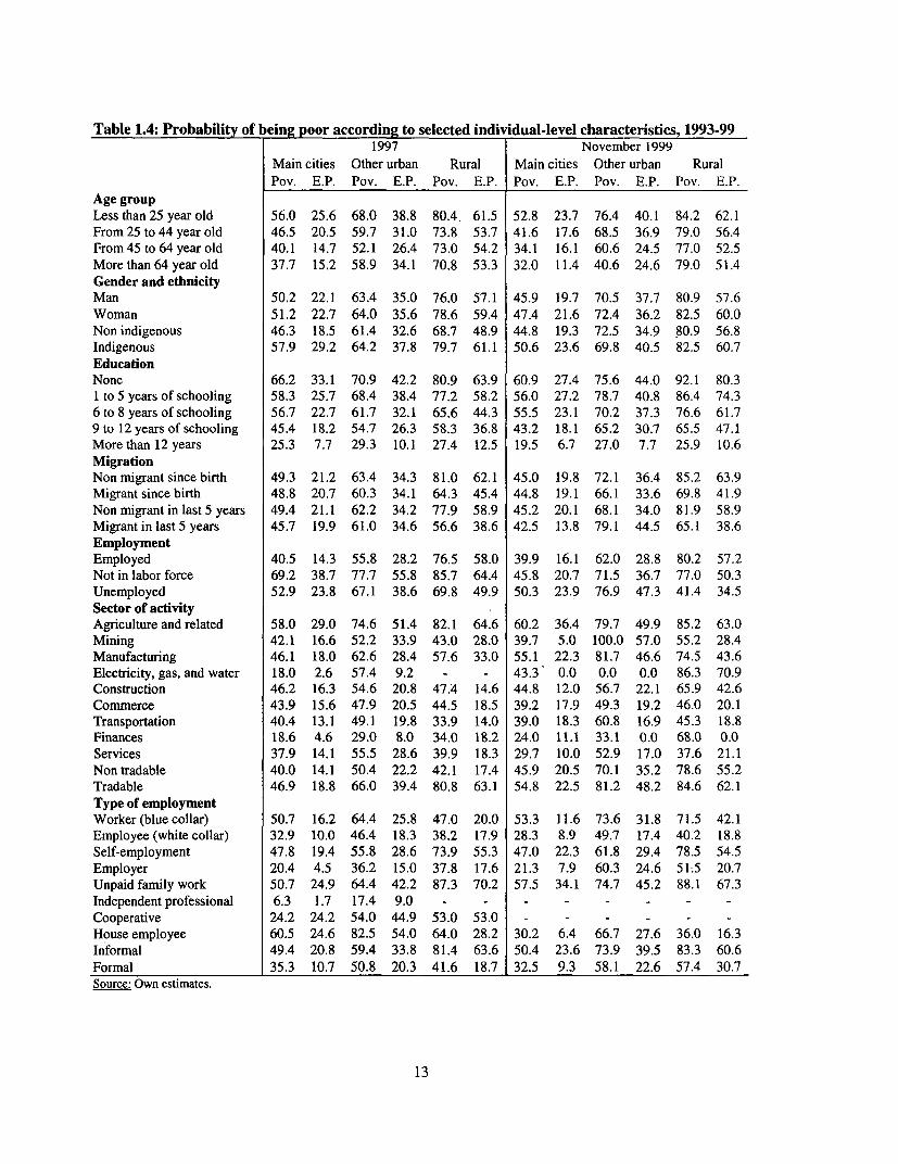
Table 1.1: Extreme and Moderate Poverty Lines in Bolivia's Departments and Cities, 1993-99 ................................. 8Table 1.2: Trend in Poverty and Extreme Poverty, 1993-99 ............................................................................ 10Table 1.3: Poverty and Extreme Poverty in Latin America, 1995-98 ......................................................................... 10Table 1.4: Probability of Being Poor According to Selected Individual-level Characteristics .................................... 13Table 1.5: Inequality for per capita income: Income shares, and Gini and Atkinson indices, 1993-99 ....................... 14Table 1.6: Decomposition of Gini for Per Capita Income by Area, 1996 and 1997 .................................................... 16Table 1.7: Decomposition by Source of Gini for Per Capita Income/Expenditures, Main Cities, 1999 ..................... 16

Table 2.1: Marginal Percentage Change in Per Capita Income Due to Demographic Variables ................................ 19Table 2.2: Marginal Percentage Change in Per Capita Income Due to Education ...................................................... 20Table 2.3: Marginal Percentage Change in Labor Income with More Education by Level, Urban Men .................... 20Table 2.4: Marginal Percentage Change in Per Capita Income Due to Employment/Underemployment ................... 22Table 2.5: Marginal Percentage Change in Per Capita Income Due to the Sector of Activity .................................... 22Table 2.6: Marginal Percentage Change in Per Capita Income Due to Other Employment Variables ........................ 23Table 2.7: Reduction in Poverty from an Increase in Employment, with and without Wage Impact, 1996 ................ 24Table 2.8: Marginal Percentage Change in Per Capita Income Due to Geographic Location ..................................... 25Table 2.9: Impact of Location on Earnings, Labor Force Participation, Health and Schooling .................................. 25Table 2.10: Variance in Province Wages, Labor Force Participation, Health and Schooling ..................................... 26Table 2.11 :Marginal Percentage Change in Per Capita Income Due to Migration ..................................................... 27Table 2.12: Marginal Percentage Change in Per Capita Income Due to Ethnicity or Language Spoken .................... 27Table 2.13: Perceived Changes in Rural Productivity in the 1990s, Focus Groups (Percentages) .............................. 29Table 2.14: Causes of Perceived Changes in Rural Productivity in the 1990s, Focus Groups (Percentages) ............. 30

Table 3.1: Share of the population poor according to unmet basic needs (NBI), 2001 census ................................... 34Table 3.2: Trend in Human Development Index and Comparison with PRSP Countries, 1980-99 ............................ 35Table 3.3: Access to Basic Infrastructure Services by Income Group (Decile) and Area, 1997 ................................. 37Table 3.4: Access to Basic Infrastructure Services by Income Group (Decile) and Area, 1999 ................................. 38Table 3.5: Percentage Increase in Rent Due to Electricity, Water and Sanitary Installation, 1998-99 ........................ 39Table 3.6: Estimating the Value of Access to Basic Infrastructure Services by Income Quintile, 1999 ..................... 40Table 3.7: Reduction in Poverty with Universal Access to Basic Infrastructure Services, 1998 ................................ 41Table 3.8: Areas Where Priority Actions are Needed According to Selected Poor Communities, 1999 .................... 45Table 3.9: Evaluation by the Poor of the Support Provided by Alternative Organizations, 1999 ............................... 47

Table 4.1: Education Sector Indicators - Primary and Secondary Levels, 1990-97 ................................................... 49Table 4.2: School Enrollment and Child Labor by Area, Income, Gender and Age, 1997 and 1999 .......................... 51Table 4.3: Monthly Expenditures for Schooling by Area and Income Level, 1999 .................................................... 52Table 4.4: Enrollment Shares in Private and public schools by Area, Income, gender and Age ................................. 53Table 4.5: Supply and Quality Measures for Public and Private Education by Level, 1996 ....................................... 54Table 4.6: Estimates of the Cost of Child Labor in Terms of Forgone Future Earnings, 1996 ................................... 56Table 4.7: Selected Health Indicators, 1989-98 ............................................................................ 58Table 4.8: Alternative Estimates of Vaccination Rates by Area and Income Group, 1999 ......................................... 58

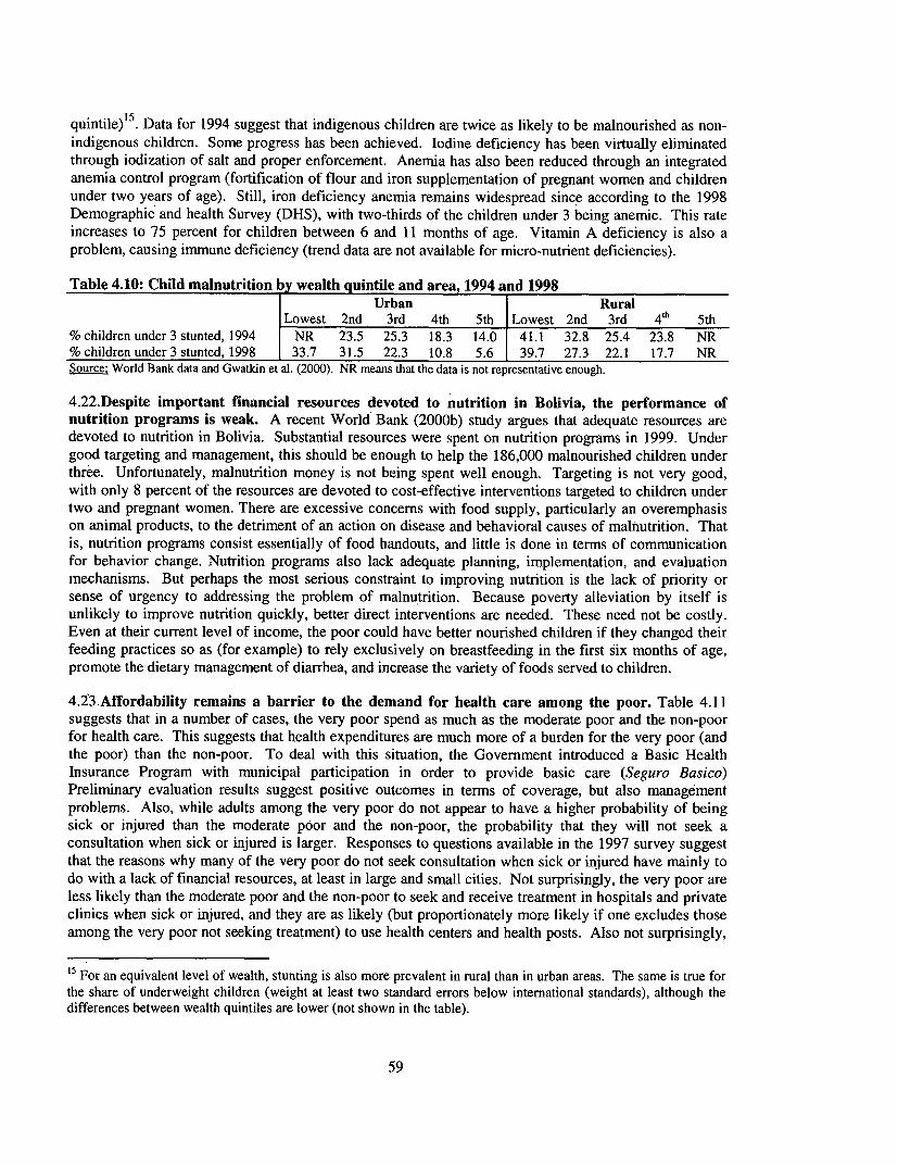
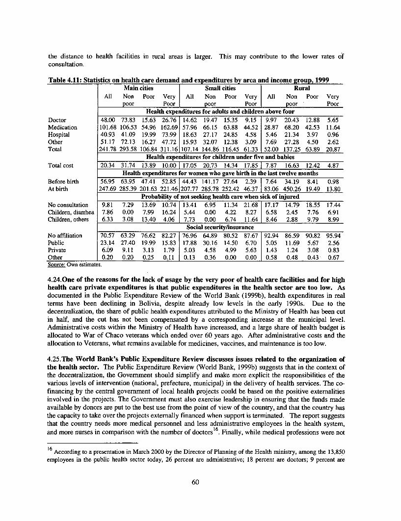
Table 4.9: Assistance Received for Birth Delivery Over the Last Twelve Months, November 1999 ......................... 58Table 4.10: Child Malnutrition by Wealth Quintile and Area, 1994 and 1998 ........................................................... 59Table 4.11: Statistics on Health Care Demand and Expenditures by Area and Income Group ................................... 60

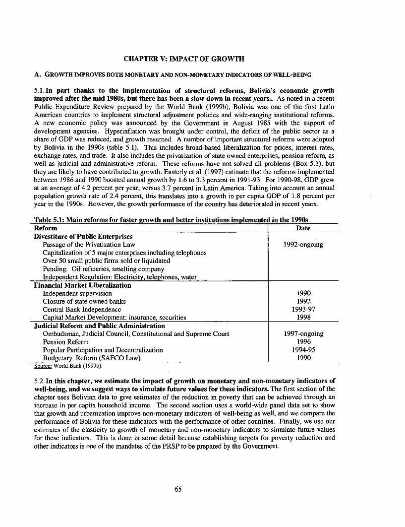
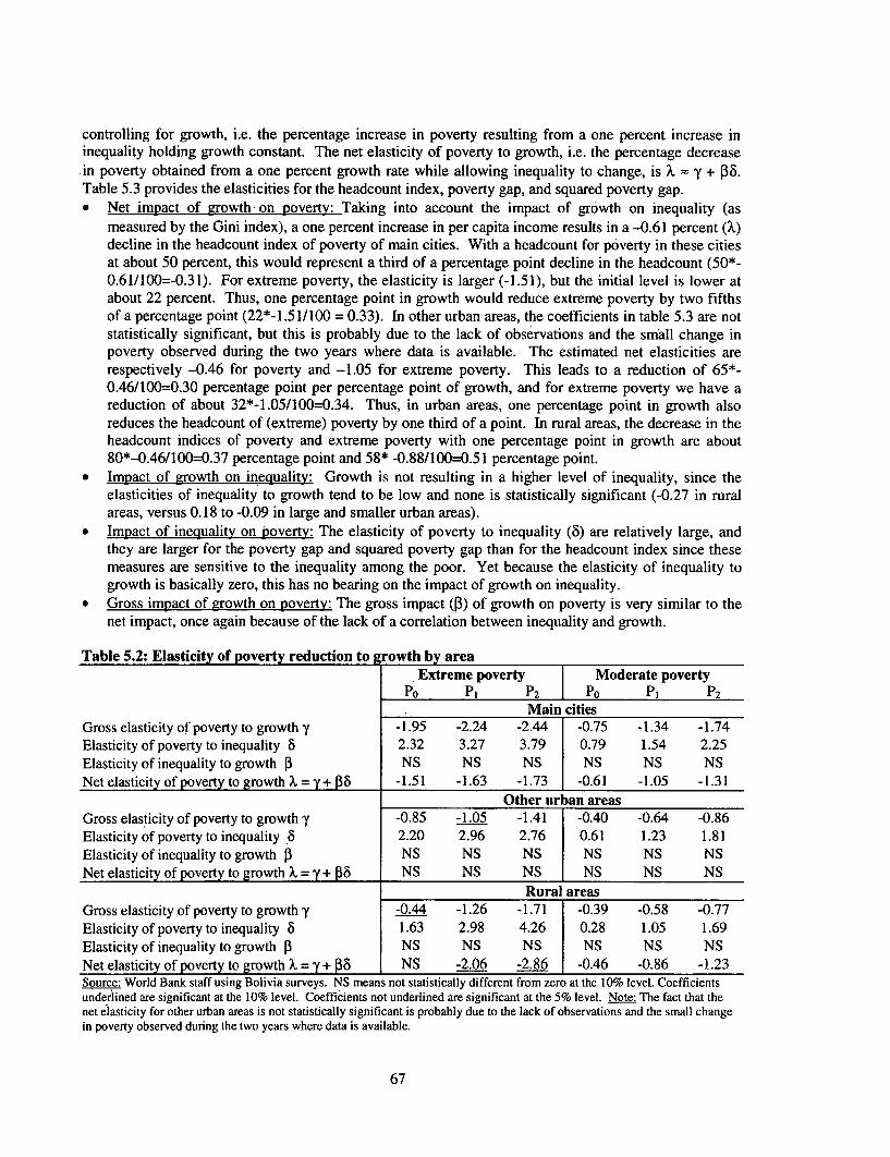
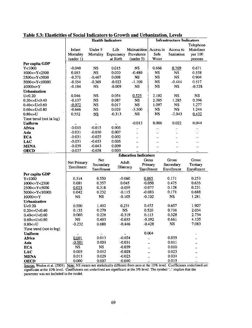
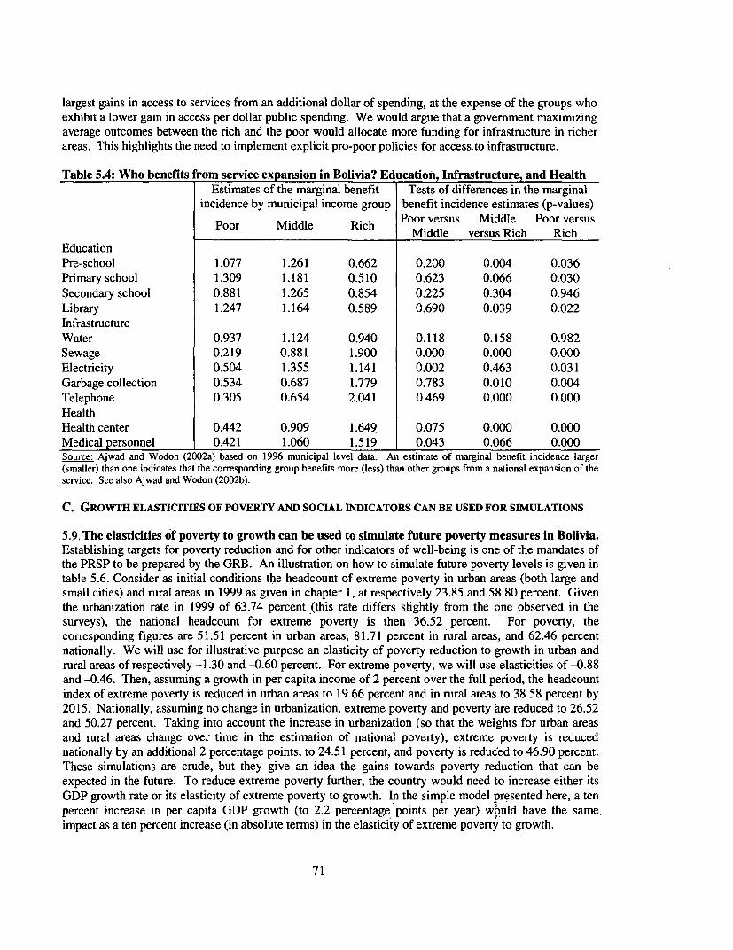
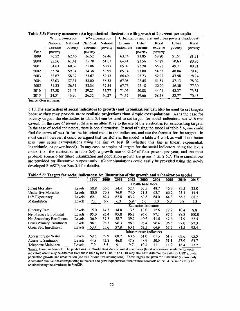
Table 5.1: Main Reforms for Faster Growth and Better Institutions Implemented in the 1990s ................................. 65Table 5.2: Elasticity of Poverty Reduction to Growth by Area ......................................................................... 67Table 5.3: Elasticity of Non-monetary Indicators to GDP Growth and Urbanization, World Panel ........................... 69Table 5.4: Who Benefits From an Service'Expansion in Bolivia? Education, Infrastructure and Health ................... 71Table 5.5: Poverty measures: A Hypothetical Illustration with Growth at 2 Percent Per Capita ................................ 72Table 5.6: Social Indicators: An Application of the Growth and Urbanization Model ............................................... 72

List of Figures

Figure ES. 1: Trends in total and social expenditures as a share of GDP ................................................................... xvFigure ES.2: Country efficiency Measures for Net Primary Enrollment and Life Expectancy ............. .................... xvi

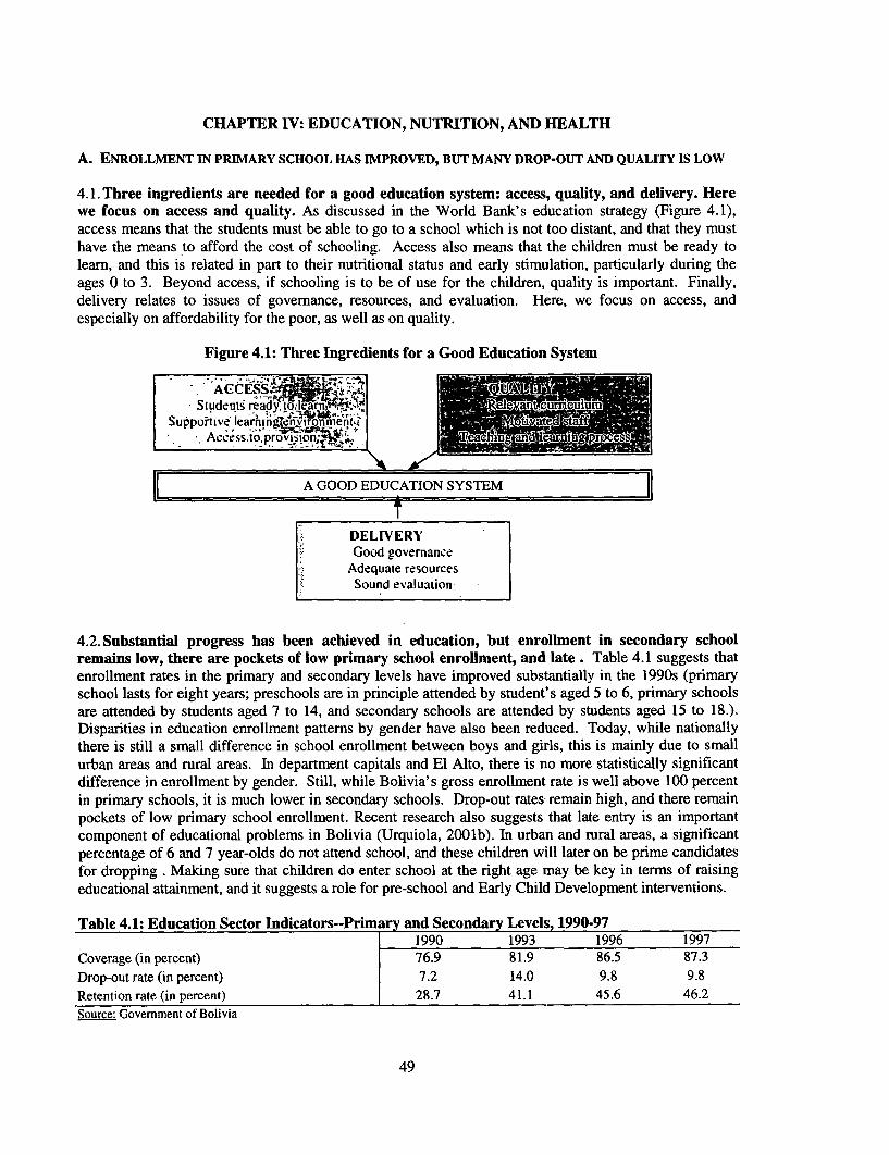
Figure 4.1: Three Ingredients for a Good Education System ......................................................................... 49

List of Boxes

Box 1.1: Aspirations and institutions: Bolivia's Human Development Report 2000 .................................................... 3Box 1.2: Data for Poverty Monitoring and Analysis in Bolivia .......................................................................... 6

Box 2.1: From the Determinants of Poverty to Policy: Suggestions from Latin America .......................................... 28

Box 3.1: Allocating Infrastructure Funds on the Basis of Need: Mexico's Experience .............................................. 43Box 3.2: Does Social Capital Matter for Poverty Reduction? ......................................................................... 46

Box 4.1: Eduction and Health Account for the Bulk of Public Social Expenditures .................................................. 50Box 4.2: PROGRESA: A Gender-Conscious Program for Education, Health and Nutrition ...................................... 62

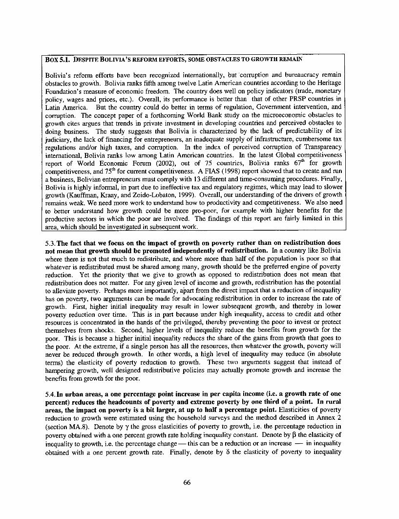
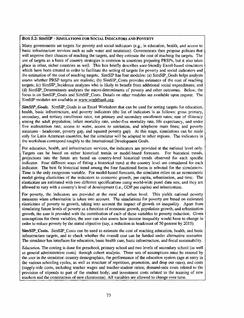
Box 5.1: Despite Bolivia's Reform Efforts, Some Obstacles to Growth Remain ....................................................... 66Box 5.2: SimSIP - Simulations for Social Indicators and Poverty ......................................................................... 73

Acknowledgements

This report was coordinated by Quentin Wodon (main author, World Bank), Wilson Jimenez (UDAPE), and JavierMonterrey (INE), with contributions from Ihsan Ajwad, Carlos Anguizola, Gabriel Gonzalez, Judith McGuire,Bernadette Ryan, and Corinne Siaens. The peer reviewers were Sarah Howden (Inter-American DevelopmentBank), Christian Jette (United Nations Development Program), and Miguel Urquiola (Universidad Catolica deBolivia). The Equity Pillar Leader for Bolivia, John Newman, and the Sector Manager for Poverty in LatinAmerica, Norman Hicks, provided overall guidance. The team expresses its deepest appreciation to the staff of INEand UDAPE for their suppprt.

BOLIVIA: POVERTY DIAGNOSTIC 2000

EXECUTIVE SUMMARY

A. THIS REPORT PROVIDES A DIAGNOSTIC OF POVERTY AND WELL-BEING IN BOLIVIA

1. This report was prepared as a contribution to Bolivia's National Dialogue H and the PovertyReduction Strategy Paper (PRSP). The report uses household surveys to give a diagnostic of poverty,human development, and access to social infrastructure. It is based on analytical work conducted by ateam comprising of staff from the National Statistical Institute (Instituto Nacional de Estadistica, INEhereafter), the inter-ministerial technical unit in charge of drafting the PRSP (Unidad de Analisis dePoliticas. Econ6micas, UDAPE hereafter), and the World Bank. The objective of this report is not toprovide recommendations on how to attack poverty in Bolivia. Policy options are discussed is the PRSPprepared by the Government (Republic of Bolivia, 2001). The report was prepared with a more limitedobjective, namely to serve as an input for the PRSP. A synthesis of the main findings was distributed bythe Government during the National Dialogue II. Now that the PRSP process has been completed, thereason for making the report publicly available in its entirety is that it contains a more detailed analysis ofpoverty in Bolivia than the synthesis distributed so far. This more detailed analysis is worthdisseminating broadly.

2. The key findings of the report are as follows:* Reduction in poverty: Nationally, in October 1999, 63 percent of the population was poor and 37

percent extreme poor, which is similar to the levels observed in 1997, but likely to be below theincidence of poverty observed in the early 1990s. Indeed, although nationally representative surveysare lacking for the early 1990s, the reduction in poverty in large cities combined with rural-urbanmigration are likely to have led to a (limited) reduction in poverty nationally. Poverty affects half ofthe population in large cities, two thirds in other urban areas, and 80 percent in rural areas. There alsoappears to have been a decrease in inequality recently, but this need not imply a long term trend.

* Complex determinants of poverty: The probability of being poor increases with the number of babiesand children, the fact of being from an indigenous population, and the fact of having a householdhead unemployed, underemployed, and/or female. Poverty decreases with education and employmentin non-agricultural occupations. Geography also affects poverty and migration is poverty reducing. Aqualitative study of farmers in the Altiplano suggests a decrease in rural productivity and strongclimatic, demographic, and environmental pressures, with little gain from most development projects.

* Progress in non-monetary indicators: From 1976 to 1992, NBI-based poverty decreased from 85.5percent to 70.9 percent nationally. The measures were reduced further to 58.6 percent in 2001.However, the gains have been achieved mainly in urban areas, while needs (and the cost of fulfillingthese needs) are larger in rural areas. The fact that NBI-based measures are improving faster thanincome-based measures is not surprising. This is a trend observed in Latin America as a whole, and itis in part due to the fact that many components of NBI-based.measures are a stock (once access to aservice is given, or a house, with good characteristics has been built, it does not need to be doneagain), while income is a flow, that has to be generated year after year. The progress in NBI-basedmeasures may also be related to the increase in social spending observed over the 1990's, and theability of improving NBI indicators through Government interventions (it is more difficult to improveincomes through labor markets interventions). Beyond NBI-based measures of poverty, progress innon-monetary indicators is also suggested by the UNDP' s Human Development Index whichincreased from 0.546 in 1980 to 0.648 in 1999. Other findings suggest scope for reducing monetarypoverty through access to public infrastructure services. Qualitative studies on the perceptions ofpoverty among the poor also suggest to pay attention to gender issues and violence.

* Room for improvement in education, health, and nutrition: Bolivia has increased public spending forthe social sectors, and some progress have been achieved. But the country still lags behind other

i

comparable countries, especially in health. Among the poor, affordability remains an issue for botheducation and health. Pre-schools appear to be a good investment. To improve quality in primaryschools, and to better fund pre-schools and secondary schools, cost-recovery mechanisms could beimplemented at the university level. The opportunity cost of child labor in terms of forgone futureearnings is large. Despite important financial resources devoted to nutrition, the performance ofnutrition programs is weak. The social investment fund does not appear to generate gains in schoolenrolment, attendance, and achievement, but it does yield positive effects on health outcomes.Impact of growth: In urban areas, a point increase in per capita income (i.e. a growth rate of onepercent) reduces the share of the population in poverty and extreme poverty by one third of a point.In rural areas, the impact on poverty is a bit larger, at up to half a percentage point. Apart fromreducing poverty, economic growth also improves non-monetary indicators of well-being such asinfant mortality, under five mortality, enrollment in secondary education, illiteracy, access to safewater, and life expectancy. Empirical work suggests that the poor may benefit more than the non-poorfrom an expansion in education services, and less than the non-poor from an expansion ininfrastructure and health services. However, we still need additional work to better understand thedeterminants of growth itself, including improvements in productivity and competitiveness. We alsoneed to better understand how growth could be more pro-poor, for example with higher benefits forthe productive sectors in which the poor are involved the most.

CHAPTER 1: THERE HAS BEEN PROGRESS TOWARDS POVERTY REDUCTION IN THE 1990S

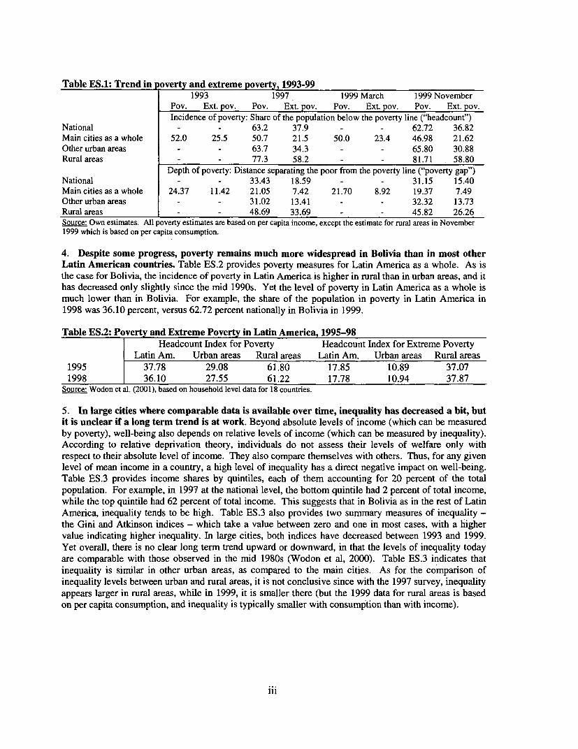
3. In the main cities, the share of the population in poverty has decreased in the 1990s. Notsurprisingly, poverty remains much higher in small cities and rural areas than in large cities. Theshares of the population living in poverty (per capita income below the cost of food and non-food needs)and extreme poverty (i.e., having a level of per capita income below the cost of basic food needs) aregiven in the top part of table ES 1. In 1997 and November 1999, we provide estimates of poverty andextreme poverty nationally, in large cities (departmental capitals and El Alto), in smaller cities and inrural areas. In 1993 and March 1999, we have surveys only for large cities. The results are as follows:* In large cities, the share of the population in poverty decreasing from 52.0 percent in 1993 to 50.0

percent in March 1999, and 47.0 percent in November 1999. A similar decline is observed for theshare of the population in extreme poverty, from 25.5 percent in 1993 to 21.62 percent in 1999.

* In other urban areas and in rural areas, there is no clear trend between 1997 and 1999 towards higheror lower poverty when alternative measures of both poverty and extreme poverty are taken intoaccount. In small urban areas for example, the share of the population living in extreme poverty hasdecreased slightly while the share of the population living in poverty has increased slightly. In ruralareas, even if the share of the rural poverty were to have increased between 1997 and 1999 assuggested in the table, the share of the population in extreme poverty has remained virtuallyunchanged. Moreover, if one takes into account the poverty gap rather than the headcount index as ameasure of poverty, so as to take into account the distance separating the poor from the poverty line,one finds that poverty actually decreased in rural areas, while it again remained stable in urban areas.

* Nationally, slightly less than two thirds of the population (62.7 percent) lives in poverty, and slightlymore than one third of the population (36.8 percent) lives in extreme poverty. There has been nomajor change in poverty and extreme poverty between October 1997 and November 1999, which isnot surprising given the lack of substantial economic growth per capita over the last two years. Still,despite the lack of nationally representative data in the early 1990s, it can be conjectured that povertydecreased thanks to the decrease in poverty in large cities and the extent of rural-urban migration. Inthe future, it will be important to continue to implement national surveys and to maximizecomparability between the surveys so as to have more confidence about the trend in poverty.

ii

Table ES.1: Trend in poverty and extreme poverty, 1993-991993 1997 1999 March 1999 November

Pov. Ext. pov. Pov. Ext. pov. Pov. Ext. pov. Pov. Ext. pov.Incidence of poverty: Share of the population below the poverty line ("headcount")

National - - 63.2 37.9 - - 62.72 36.82Main cities as a whole 52.0 25.5 50.7 21.5 50.0 23.4 46.98 21.62Other urban areas - - 63.7 34.3 - - 65.80 30.88Rural areas - - 77.3 58.2 - - 81.71 58.80

Depth of poverty: Distance separating the poor from the poverty line ("poverty gap")National - - 33.43 18.59 - - 31.15 15.40Main cities as a whole 24.37 11.42 21.05 7.42 21.70 8.92 19.37 7.49Other urban areas - - 31.02 13.41 - - 32.32 13.73Rural areas - - 48.69 33.69 - - 45.82 26.26Source: Own estimates. All poverty estimates are based on per capita income, except the estimate for rural areas in November1999 which is based on per capita consumption.

4. Despite some progress, poverty remains much more widespread in Bolivia than in most otherLatin American countries. Table ES.2 provides poverty measures for Latin America as a whole. As isthe case for Bolivia, the incidence of poverty in Latin America is higher in rural than in urban areas, and ithas decreased only slightly since the mid 1990s. Yet the level of poverty in Latin America as a whole ismuch lower than in Bolivia. For example, the share of the population in poverty in Latin America in1998 was 36.10 percent, versus 62.72 percent nationally in Bolivia in 1999.

Table ES.2: P verty and Extreme Poverty in Latin America, 1995-98Headcount Index for Poverty Headcount Index for Extreme Poverty

Latin Am. Urban areas Rural areas Latin Am. Urban areas Rural areas1995 37.78 29.08 61.80 17.85 10.89 37.071998 36.10 27.55 61.22 17.78 10.94 37.87

Source: Wodon et al. (2001), based on household level data for 18 countries.

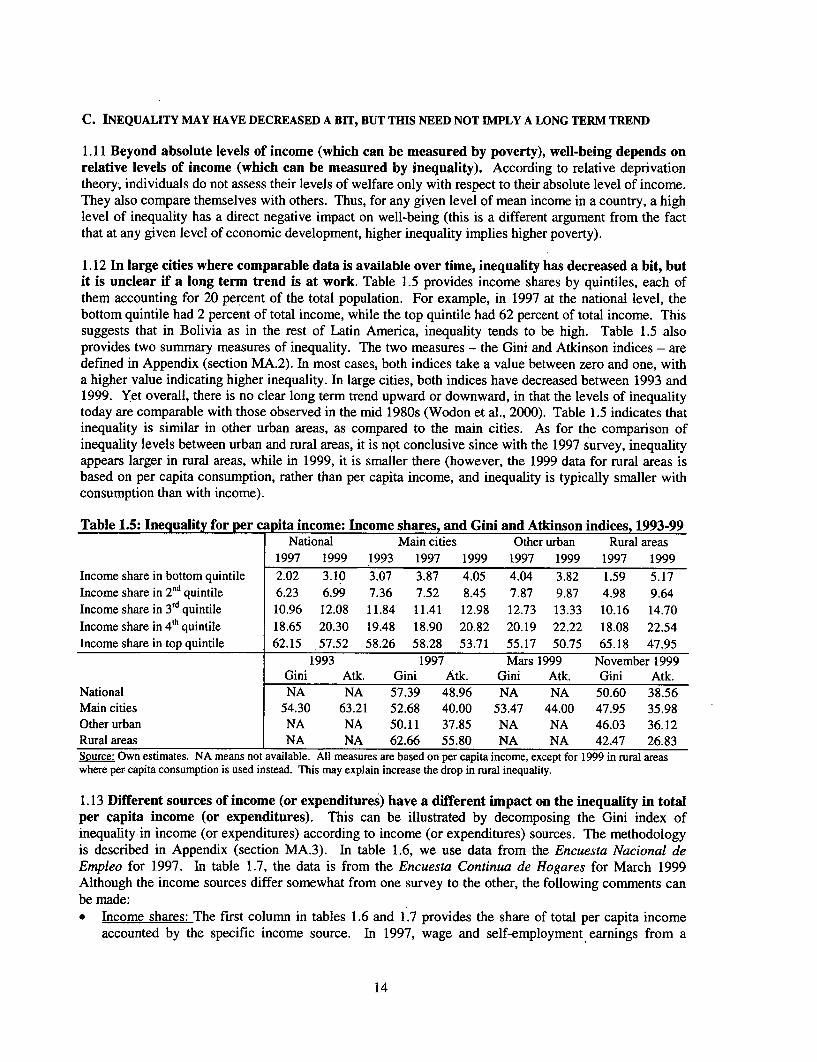
5. In large cities where comparable data is available over time, inequality has decreased a bit, butit is unclear if a long term trend is at work. Beyond absolute levels of income (which can be measuredby poverty), well-being also depends on relative levels of income (which can be measured by inequality).According to relative deprivation theory, individuals do not assess their levels of welfare only withrespect to their absolute level of income. They also compare themselves with others. Thus, for any givenlevel of mean income in a country, a high level of inequality has a direct negative impact on well-being.Table ES.3 provides income shares by quintiles, each of them accounting for 20 percent of the totalpopulation. For example, in 1997 at the national level, the bottom quintile had 2 percent of total income,while the top quintile had 62 percent of total income. This suggests that in Bolivia as in the rest of LatinAmerica, inequality tends to be high. Table ES.3 also provides two summary measures of inequality -the Gini and Atkinson indices - which take a value between zero and one in most cases, with a highervalue indicating higher inequality. In large cities, both indices have decreased between 1993 and 1999.Yet overall, there is no clear long term trend upward or downward, in that the levels of inequality todayare comparable with those observed in the mid 1980s (Wodon et al, 2000). Table ES.3 indicates thatinequality is similar in other urban areas, as compared to the main cities. As for the comparison ofinequality levels between urban and rural areas, it is not conclusive since with the 1997 survey, inequalityappears larger in rural areas, while in 1999, it is smaller there (but the 1999 data for rural areas is basedon per capita consumption, and inequality is typically smaller with consumption than with income).

iii

Table ES.3: Inequality for per capita income: Income shares, and Gini/Atkinson indices, 1993-99National Main cities Other urban Rural areas

1997 1999 1993 1997 1999 1997 1999 1997 1999Income share in bottom quintile 2.02 3.10 3.07 3.87 4.05 4.04 3.82 1.59 5.17Income share in 2nd quintile 6.23 6.99 7.36 7.52 8.45 7.87 9.87 4.98 9.64Income share in 3rdquintile 10.96 12.08 11.84 11.41 12.98 12.73 13.33 10.16 14.70Income share in 4h quintile 18.65 20.30 19.48 18.90 20.82 20.19 22.22 18.08 22.54Income share in top quintile 62.15 57.52 58.26 58.28 53.71 55.17 50.75 65.18 47.95

1993 1997 Mars 1999 November 1999Gini Atk. Gini Atk. Gini Atk. Gini Atk.

National NA NA 57.39 48.96 NA NA 50.60 38.56Main cities 54.30 63.21 52.68 40.00 53.47 44.00 47.95 35.98Other urban NA NA 50.11 37.85 NA NA 46.03 36.12Rural areas NA NA 62.66 55.80 NA NA 42.47 26.83Source: Own estimates. NA means not available. All measures are based on per capita income, except for 1999 in rural areaswhere per capita consumption is used instead. This may explain increase the drop in rural inequality.

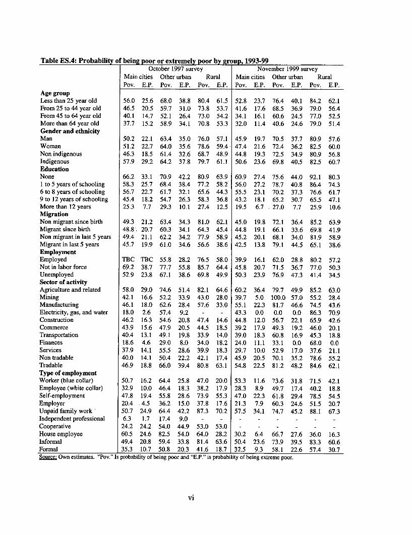
6. As expected, there are large differences in the incidence of poverty between various groups.Table ES.4 gives probabilities of being poor and extremely poor according to various characteristics.* Age among the adult population: In most cases, the probability of being poor decreases as the

individual gets older. In November 1999 for example, rural individuals aged less than 25 years havea probability of being in extreme poverty of 62.1 percent, versus 51.4 percent for those aged 64 orolder. In small urban cities, the corresponding probabilities are 40.1 and 24.6 percent. In main cities,the probabilities are 23.7 and 11.4 percent. In a few cases however, individuals above 64 years of ageare more likely to be poor than individuals aged between 45 and 64. None of these results aresurprising given that the profile of poverty is linked to the life cycle of earnings. Yet the profile ofpoverty by age depends on methodological choices, so that one should be cautious before makingpolicy recommendations or assuming that social programs targeting the elderly are not warranted.

* Gender: In both urban and rural areas, the incidence of poverty is slightly higher for women (andgirls) than for men (and boys). The differences are systematic, but they are very small. They may bedue to the fact that female headed households, which typically have a higher share of women asmembers since the head is a woman and there is no spouse, have a higher probability of being poor.

* Ethnicity: Ethnicity can be captured using either the language spoken as an indicator of whether theindividual is from an indigenous population or not (in the 1997 survey) or the self-affiliation of theindividual (in the November 1999 survey). In 1997, those not speaking Spanish or a foreign languagesuch as English have been classified as being indigenous (the reference population is slightly smallerthan the full sample because the questions is not asked to very young children.) Not surprisingly,indigenous populations are more likely to be poor than non-indigenous populations. This is observedin both 1997 and 1999, although the differences tend to be smaller in the 1999 survey. Note thatwhile the indigenous populations represent more than two thirds of the rural population, they accountfor less than a third of the population living in the main cities and other urban areas.

* Education: The lower the level of education, the higher the probability of being poor. For example, in1999, in the main cities, individuals ten years or older with no education at all had a probability ofbeing poor of 60.9 percent, as compared to 19.5 percent for individuals with more than 12 years ofschooling. The same pattern can be observed in other urban areas and in rural areas, but with levelsof poverty and extreme poverty by education group a few percentage points higher.

* Migration of the head: Two types of migration are considered: whether the individual lives in adifferent place than its place of birth, and whether the individual has been living in its current place ofresidence for less than five years. In the main cities and in other urban areas, those who havemigrated since birth tend to be on par with individuals living in the same area since their birth. Inrural areas, those who migrated since their birth tend to be better off than those who did not migrate.

iv

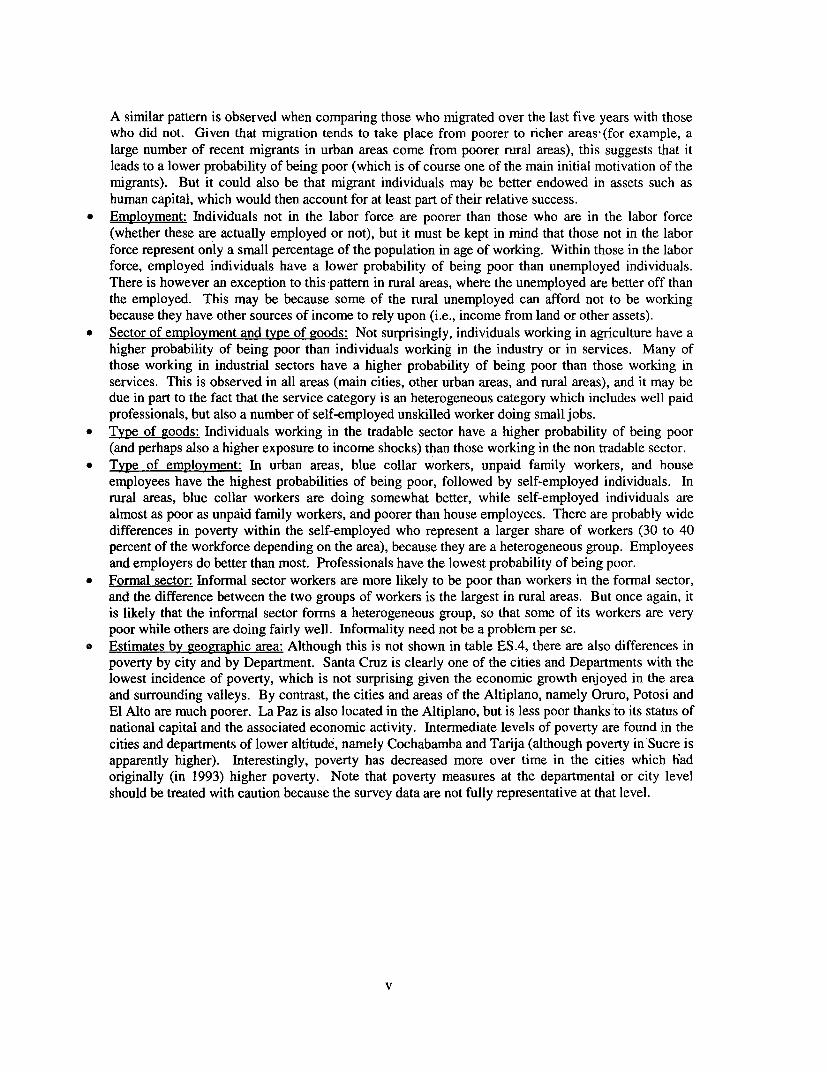
A similar pattern is observed when comparing those who migrated over the last five years with thosewho did not. Given that migration tends to take place from poorer to richer areas' (for example, alarge number of recent migrants in urban areas come from poorer rural areas), this suggests that itleads to a lower probability of being poor (which is of course one of the main initial motivation of themigrants). But it could also be that migrant individuals may be better endowed in assets such ashuman capital, which would then account for at least part of their relative success.

* Employment: Individuals not in the labor force are poorer than those who are in the labor force(whether these are actually employed or not), but it must be kept in mind that those not in the laborforce represent only a small percentage of the population in age of working. Within those in the laborforce, employed individuals have a lower probability of being poor than unemployed individuals.There is however an exception to this pattern in rural areas, where the unemployed are better off thanthe employed. This may be because some of the rural unemployed can afford not to be workingbecause they have other sources of income to rely upon (i.e., income from land or other assets).

* Sector of employment and type of goods: Not surprisingly, individuals working in agriculture have ahigher probability of being poor than individuals working in the industry or in services. Many ofthose working in industrial sectors have a higher probability of being poor than those working inservices. This is observed in all areas (main cities, other urban areas, and rural areas), and it may bedue in part to the fact that the service category is an heterogeneous category which includes well paidprofessionals, but also a number of self-employed unskilled worker doing small jobs.

* Type of goods: Individuals working in the tradable sector have a higher probability of being poor(and perhaps also a higher exposure to income shocks) than those working in the non tradable sector.

* Type of employment: In urban areas, blue collar workers, unpaid family workers, and houseemployees have the highest probabilities of being poor, followed by self-employed individuals. Inrural areas, blue collar workers are doing somewhat better, while self-employed individuals arealmost as poor as unpaid family workers, and poorer than house employees. There are probably widedifferences in poverty within the self-employed who represent a larger share of workers (30 to 40percent of the workforce depending on the area), because they are a heterogeneous group. Employeesand employers do better than most. Professionals have the lowest probability of being poor.

* Formal sector: Informal sector workers are more likely to be poor than workers in the formal sector,and the difference between the two groups of workers is the largest in rural areas. But once again, itis likely that the informal sector forms a heterogeneous group, so that some of its workers are verypoor while others are doing fairly well. Informality need not be a problem per se.

* Estimates by geographic area: Although this is not shown in table ES.4, there are also differences inpoverty by city and by Department. Santa Cruz is clearly one of the cities and Departments with thelowest incidence of poverty, which is not surprising given the economic growth enjoyed in the areaand surrounding valleys. By contrast, the cities and areas of the Altiplano, namely Oruro, Potosi andEl Alto are much poorer. La Paz is also located in the Altiplano, but is less poor thanks to its status ofnational capital and the associated economic activity. Intermediate levels of poverty are found in thecities and departments of lower altitude, namely Cochabamba and Tarija (although poverty in Sucre isapparently higher). Interestingly, poverty has decreased more over time in the cities which h'adoriginally (in 1993) higher poverty. Note that poverty measures at the departmental or city levelshould be treated with caution because the survey data are not fully representative at that level.

v

Table ES.4: Probability of being poor or extremely poor by gr oup, 1993-99October 1997 survey November 1999 survey

Main cities Other urban Rural Main cities Other urban RuralPov. E.P. Pov. E.P. Pov. E.P. Pov. E.P. Pov. E.P. Pov. E.P.

Age groupLess than 25 year old 56.0 25.6 68.0 38.8 80.4 61.5 52.8 23.7 76.4 40.1 84.2 62.1From 25 to 44 year old 46.5 20.5 59.7 31.0 73.8 53.7 41.6 17.6 68.5 36.9 79.0 56.4From 45 to 64 year old 40.1 14.7 52.1 26.4 73.0 54.2 34.1 16.1 60.6 24.5 77.0 52.5More than 64 year old 37.7 15.2 58.9 34.1 70.8 53.3 32.0 11.4 40.6 24.6 79.0 51.4Gender and ethnicityMan 50.2 22.1 63.4 35.0 76.0 57.1 45.9 19.7 70.5 37.7 80.9 57.6Woman 51.2 22.7 64.0 35.6 78.6 59.4 47.4 21.6 72.4 36.2 82.5 60.0Non indigenous 46.3 18.5 61.4 32.6 68.7 48.9 44.8 19.3 72.5 34.9 80.9 56.8Indigenous 57.9 29.2 64.2 37.8 79.7 61.1 50.6 23.6 69.8 40.5 82.5 60.7EducationNone 66.2 33.1 70.9 42.2 80.9 63.9 60.9 27.4 75.6 44.0 92.1 80.31 to 5 years of schooling 58.3 25.7 68.4 38.4 77.2 58.2 56.0 27.2 78.7 40.8 86.4 74.36 to 8 years of schooling 56.7 22.7 61.7 32.1 65.6 44.3 55.5 23.1 70:2 37.3 76.6 61.79 to 12 years of schooling 45.4 18.2 54.7 26.3 58.3 36.8 43.2 18.1 65.2 30.7 65.5 47.1More than 12 years 25.3 7.7 29.3 10.1 27.4 12.5 19.5 6.7 27.0 7.7 25.9 10.6MigrationNon migrant since birth 49.3 21.2 63.4 34.3 81.0 62.1 45.0 19.8 72.1 36.4 85.2 63.9Migrant since birth 48.8. 20.7 60.3 34.1 64.3 45.4 44.8 19.1 66.1 33.6 69.8 41.9Non migrant in last 5 years 49.4 21.1 62.2 34.2 77.9 58.9 45.2 20.1 68.1 34.0 81.9 58.9Migrant in last 5 years 45.7 19.9 61.0 34.6 56.6 38.6 42.5 13.8 79.1 44.5 65.1 38.6EmploymentEmployed TBC TBC 55.8 28.2 76.5 58.0 39.9 16.1 62.0 28.8 80.2 57.2Not in labor force 69.2 38.7 77.7 55.8 85.7 64.4 45.8 20.7 71.5 36.7 77.0 50.3Unemployed 52.9 23.8 67.1 38.6 69.8 49.9 50.3 23.9 76.9 47.3 41.4 34.5Sector of activityAgriculture and related 58.0 29.0 74.6 51.4 82.1 64.6 60.2 36.4 79.7 49.9 85.2 63.0Mining 42.1 16.6 52.2 33.9 43.0 28.0 39.7 5.0 100.0 57.0 55.2 28.4Manufacturing 46.1 18.0 62.6 28.4 57.6 33.0 55.1 22.3 81.7 46.6 74.5 43.6Electricity, gas, and water 18.0 2.6 57.4 9.2 - - 43.3 0.0 0.0 0.0 86.3 70.9Construction 46.2 16.3 54.6 20.8 47.4 14.6 44.8 12.0 56.7 22.1 65.9 42.6Commerce 43.9 15.6 47.9 20.5 44.5 18.5 39.2 17.9 49.3 19.2 46.0 20.1Transportation 40.4 13.1 49.1 19.8 33.9 14.0 39.0 18.3 60.8 16.9 45.3 18.8Finances 18.6 4.6 29.0 8.0 34.0 18.2 24.0 11.1 33.1 0.0 68.0 0.0Services 37.9 14.1 55.5 28.6 39.9 18.3 29.7 10.0 52.9 17.0 37.6 21.1Non tradable 40.0 14.1 50.4 22.2 42.1 17.4 45.9 20.5 70.1 35.2 78.6 55.2Tradable 46.9 18.8 66.0 39.4 80.8 63.1 54.8 22.5 81.2 48.2 84.6 62.1Type of employmentWorker (blue collar) 50.7 16.2 64.4 25.8 47.0 20.0 53.3 11.6 73.6 31.8 71.5 42.1Employee (white collar) 32.9 10.0 46.4 18.3 38.2 17.9 28.3 8.9 49.7 17.4 40.2 18.8Self-employment 47.8 19.4 55.8 28.6 73.9 55.3 47.0 22.3 61.8 29.4 78.5 54.5Employer 20.4 .4.5 36.2 15.0 37.8 17.6 21.3 7.9 60.3 24.6 51.5 20.7Unpaid family work' 50.7 24.9 64.4 42.2 87.3 70.2 57.5 34.1 74.7 45.2 88.1 67.3Independent professional 6.3 1.7 17.4 9.0 - - - - - - - -Cooperative 24.2 24.2 54.0 44.9 53.0 53.0 - - - - - -House employee 60.5 24.6 82.5 54.0 64.0 28.2 30.2 6.4 66.7 27.6 36.0 16.3Informal 49.4 20.8 59.4 33.8 81.4 63.6 50.4 23.6 73.9 39.5 83.3 60.6Formal 35.3 10.7 50.8 20.3 41.6 18.7 32.5 9.3 58.1 22.6 57.4 30.7Source: Own estimates. "Pov." Is probability of being poor and "E.P." is probability of being extreme poor.

vi

CHAPTER II: A LARGE NUMBER OF VARIABLES AFFECT PER CAPITA INCOME AND POVERTY

7. Beyond knowing the probability of being poor of various household groups, it is useful to knowthe impact of household and individual characteristics on per capita income, and thereby poverty.Poverty profiles such as the one presented in table ES.4 give the probability of being poor according tovarious characteristics, for example the area in which a household lives or the level of education of thehousehold head. The problem with poverty profiles is that they cannot be used to assess with precisionwhat are the determinants of poverty. For example, the fact that households in some areas have a lowerprobability of being poor than households in other areas may have nothing to do with the characteristicsof the areas in which the household lives. The differences in poverty rates between areas may be due todifferences in the characteristics of the households living in the various areas, rather than to differences inthe characteristics of the areas themselves. To sort out the determinants of poverty and the impact of anyone variable on the per capita income (and thereby the probability of being poor) holding constant allother variables, regressions are needed. The results of such regressions are summarized here.

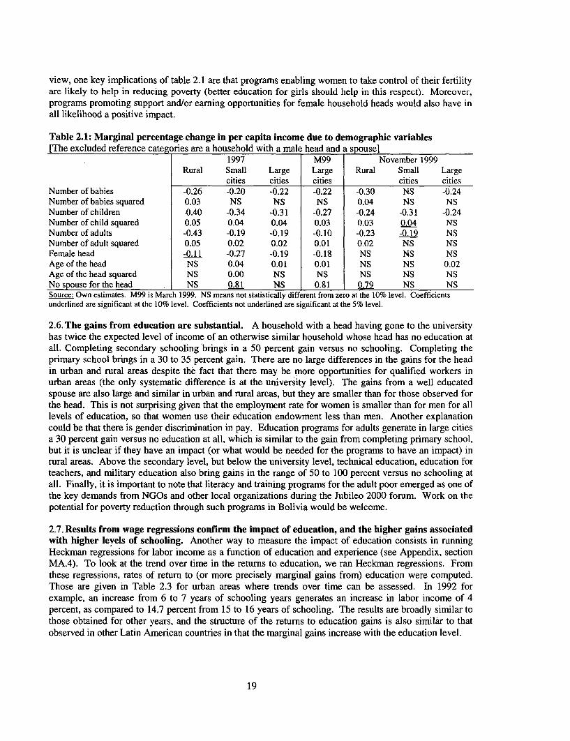
8. Poverty increases with the number of babies and children in the household. It decreases withthe age of the head. It is significantly higher in households with female heads. Controlling for othervariables, households with a larger the number of babies and children have a lower level of per capitaconsumption, and thereby a higher the probability of being poor. Somewhat surprisingly, having a largernumber of adults in the household increases the probability of being poor, which may suggest that theadditional adults (beyond the head and the spouse) are not working. It can also be seen in the regressionsthat households with younger heads are more likely to be poor, and that urban households whose head hasno spouse are less likely to be poor (probably because controlling for female headship, a large number ofheads without spouse are single males whose per capita income does not have to be shared with otherfamily members.) Finally, in many cases, female headed households have per capita income levels lowerthan male headed households. From a policy point of view, one key implications of these results is thatprograms enabling women to take control of their fertility are likely to help in reducing poverty (bettereducation for girls should help in this respect). Moreover, programs promoting support and/or betterearning opportunities for female household heads would also have in all, likelihood a positive impact.

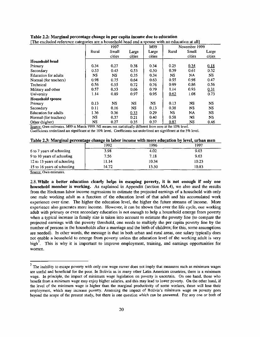
9. The income gains from education are substantial, but not large enough to emerge from povertywith a single income earner per family. A household with a head having gone to the university hastwice the expected level of per capita income of an otherwise similar household whose head has noeducation at all. A head having completed secondary schooling brings for its household in a 50 percentgain versus no schooling. A head having completed primary school brings in a 30 to 35 percent gainversus no schooling. There are no large differences in the gains from the education of the head in urbanand rural areas despite the fact that there may be more opportunities for qualified workers in urban areas(the only systematic difference between urban and rural areas are observed at the university level, withurban returns being higher). The gains from a well educated spouse are also large and similar in urbanand rural areas, but they are somewhat smaller than for those observed for the education of the head. Thisis not surprising given that the employment rate for women is smaller than for men for all levels ofeducation, so that women use their education less than men in an earnings capacity. Another explanationcould be that there is some gender discrimination in pay, but this would have be to corroborated byadditional evidence. Education programs for adults generate in large cities a 30 percent gain versus noeducation at all, which is similar to the gain from completing primary school, but it is unclear if they havean impact (or what would be needed for the programs to have an impact) in rural areas. Above thesecondary level, but below the university level, technical education, education for teachers, and military

education also bring gains in the range of 50 to 100 percent versus no schooling at all. All these resultssupport the emphasis. placed on education as a long-term strategy for poverty reduction. It is alsoimportant to note that literacy and training programs for the adult poor emerged as one of the keydemands from NGOs and other local organizations during the Jubileo 2000 forum. Work on the potential

vii

for poverty reduction through such programs in Bolivia would be welcome. Now, while a bettereducation clearly helps in escaping poverty, it is not enough if only one household member is working.One working adult with primary or even secondary education is not enough to help a household emergefrom poverty when a typical increase in family size over the life cycle is taken into account. This is whyit is important to improve employment, training, and earnings opportunities for youth and women.

10. Employment patterns have large impacts on per capita income and thereby on poverty.* Unemployment and underemployment: Not working (e.g., not being in the labor force) does not

reduce per capita income, perhaps because those who can afford not to work are better off than thosewho must work. By contrast, having a head unemployed or underemployed reduces per capitaincome. A head or spouse with a secondary occupation leads to an increase in per capita income.

* Sector of activity: Households with adults working in the agriculture sector tend to be poorer thanhouseholds with heads employed in industry or services. This is observed for both the head and thespouse. Those employed in the service industry often do better than those employed in agriculture,but they fare less well than those employed in industries. This may reflect the fact that the servicessector is heterogeneous, with well paid professional and informal sector workers lumped together.

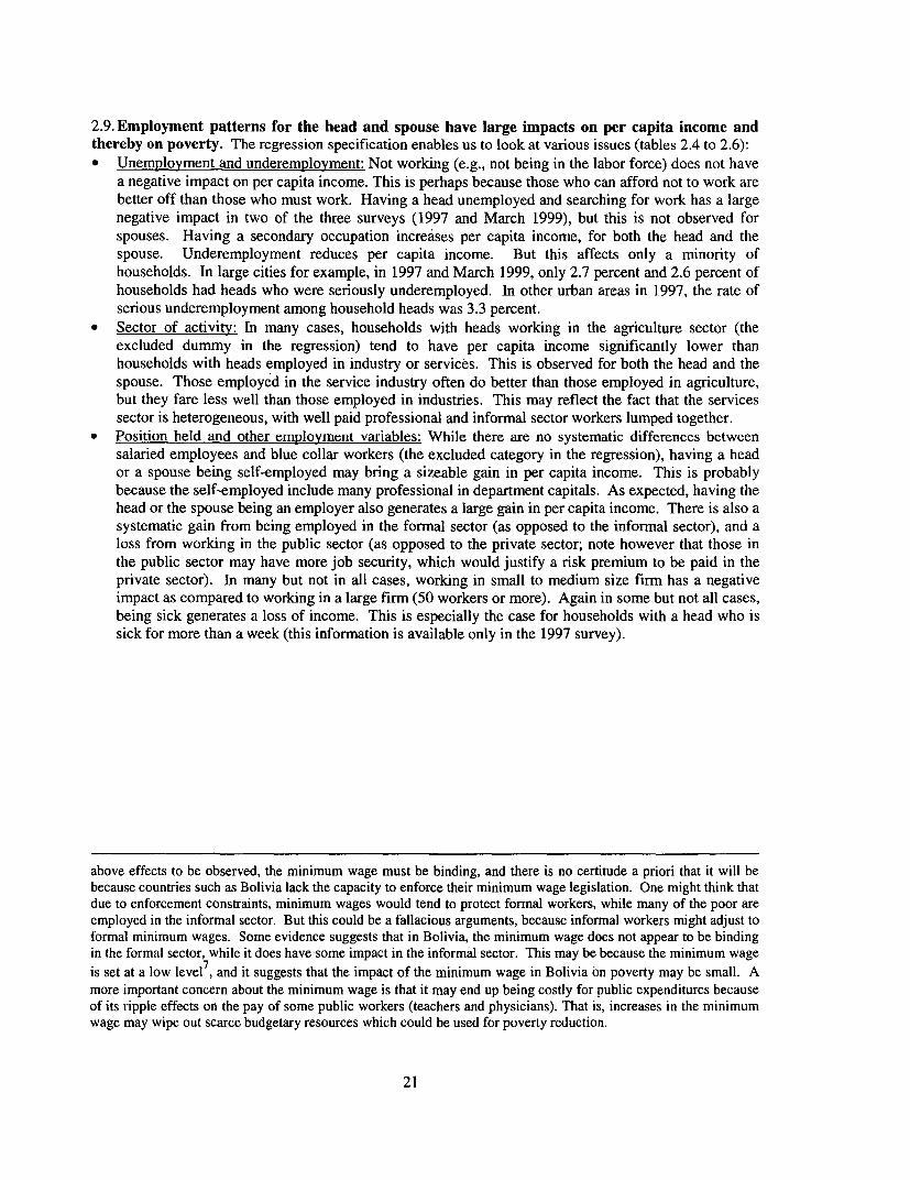
* Position held and other employment variables: While there are no systematic differences betweensalaried employees and blue collar workers, having a head or a spouse being self-employed brings asizeable gain in per capita income. Having the head or the spouse being an employer brings an evenlarger gain. There is a gain from being employed in the formal sector (as opposed to the informalsector), and a loss from working in the public sector (as opposed to the private sector; note howeverthat those in the public sector may have more job security, which would justify a risk premium to bepaid in the private sector). In many but not in all cases, working in small to medium size firm has anegative impact as compared to working in a large firm (50 workers or more). Again in some but notall cases, being sick generates a loss of income. This is especially the case for households with a headwho is sick for more than a week (this information is available only in the 1997 survey).

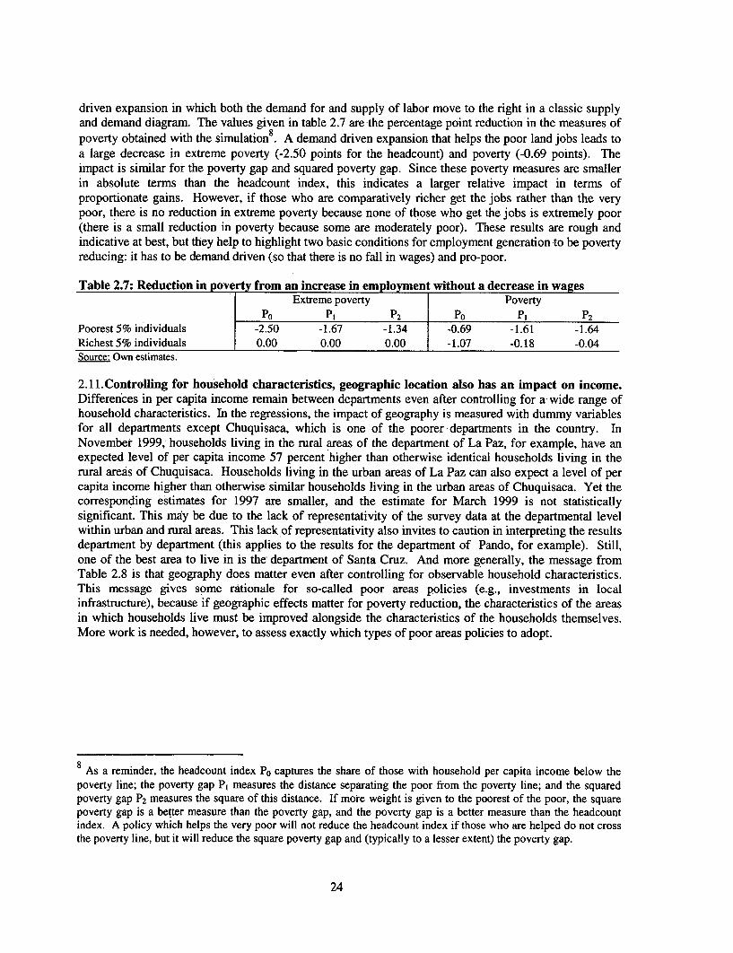
11. More employment opportunities would not eradicate poverty, but it would help to reducepoverty, provided the rise in employment is demand driven and pro-poor. Unemployment andunderemployment patterns have an impact on poverty in Bolivia at the household level, but this does notinform us of their impact at the aggregate level. To assess what would be the impact of an increase inemployment on aggregate poverty, we ran simple simulations. Among the urban adult (age 25 to 60)male population that is not earning labor income in the survey, we selected individuals to whom we gavejobs. We give the jobs to either the poorest or the richest (according to their per capita income)unemployed individuals in the sample. For these individuals, we predict earnings corresponding to theireducation and experience. The total number of individuals put to work in the simulations is equal to fivepercent of the urban adult male population at work in the survey. We assume that there is no decrease inwages when more adults are employed (the supply and demand curves for labor shift to the right jointly).It turns out that poverty reduction takes place only if poor household benefit from the job creation.

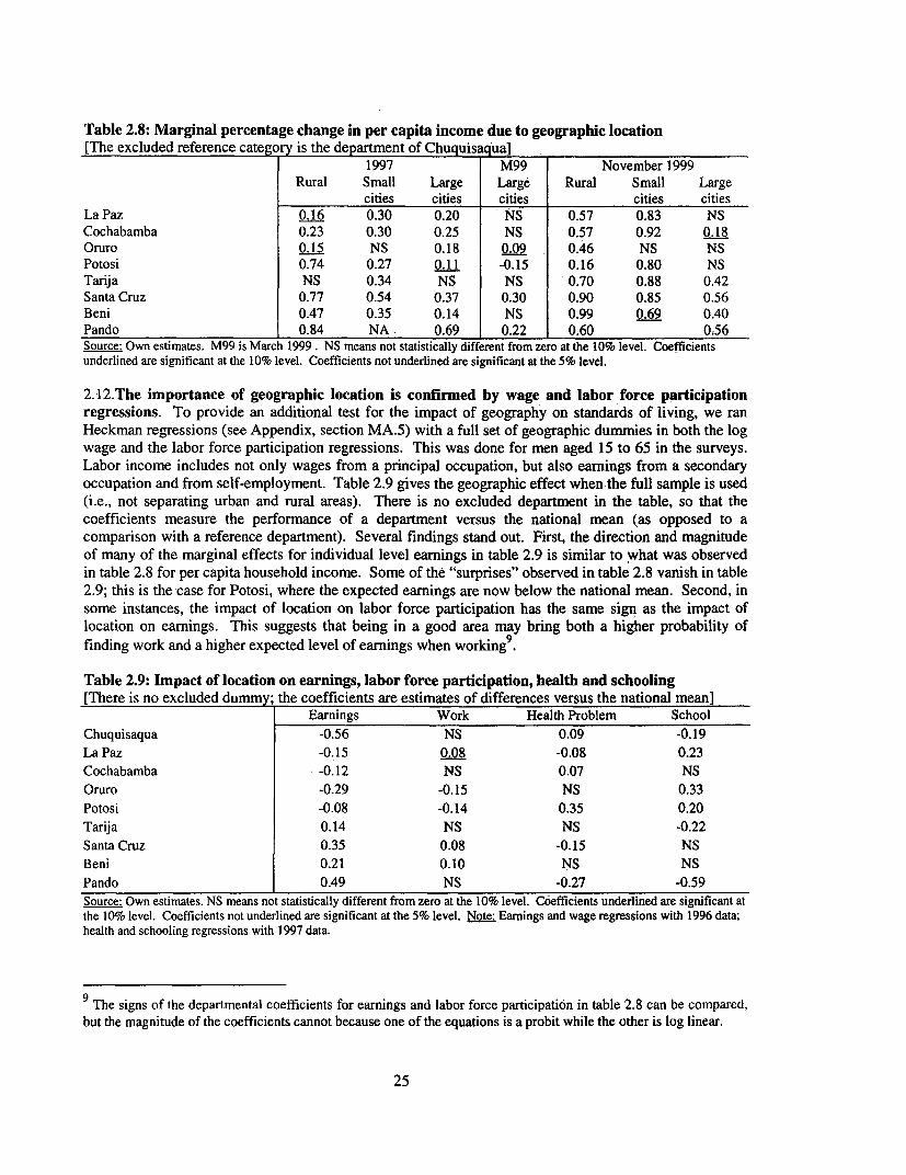
12. Geographic location also has an impact on poverty. Differences in per capita income remainbetween departments even after controlling for a wide range of household characteristics. In November1999 for example, households living in the rural areas of the department of La Paz have an expected levelof per capita income 20 percent higher than otherwise identical households living in the rural areas ofChuquisaca. Households living in the urban areas of La Paz can expect a level of per capita income from57 percent (in the city of La Paz) to 83 percent (in other urban areas of the department) than otherwisesimilar households living in the urban areas of Chuquisaca. Beyond this and other examples (such as thefact that households living in is the department of Santa Cruz are better off), the message is thatgeographic location matters. This gives some rationale for so-called poor areas policies (e.g., investmentsin local infrastructure), because if geographic effects matter for poverty reduction, the characteristics ofthe areas in which households live must be improved alongside the characteristics of the households

viii

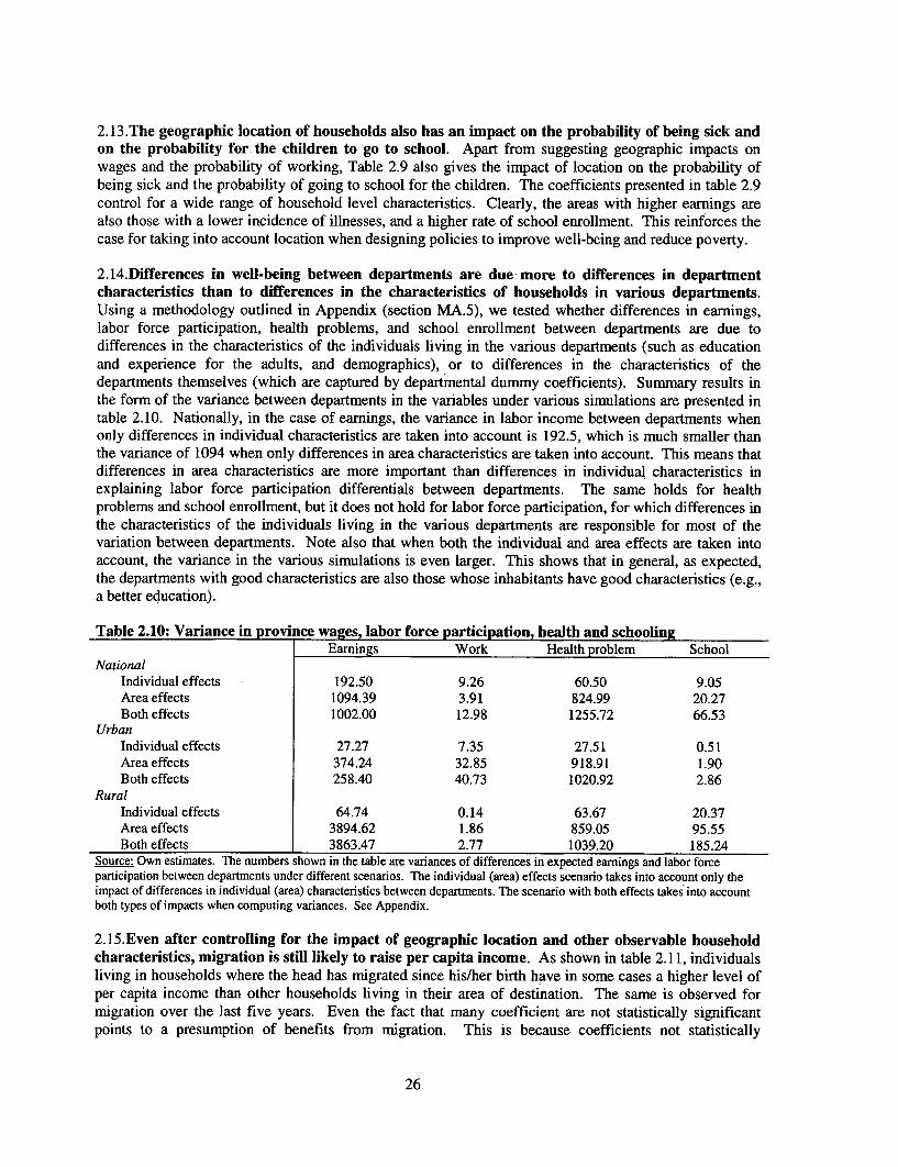
themselves. More work is needed, however, to assess exactly which types of poor areas policies to adopt.Apart from its impact on per capita income (via labor force participation and wages), geographic locationalso has a large impact on the probability of being ill, and the probability for children to go to school.Controlling for other variables, the areas with higher earnings are also those with a lower incidence ofillnesses, and a higher rate of school enrollment. This further reinforces the case for taking into accountregional development when designing policies to improve well-being and reduce poverty.

13. Even after controlling for the impact of geographic location and other observable householdcharacteristics, migration is still likely to raise per capita income. Individuals living in householdswhere the head has migrated since his/her birth have in some cases a higher level of per capita incomethan other households living in their area of destination. The same is observed for migration over the lastfive years. Even when there is no statistically significant difference between the per capita income ofmigrants and non-migrants at the place of destination, the fact that those who have migrated in the recentpast do as well as those who have lived there for more than five years suggests benefits from migration,simply because those who have migrated typically come from less favorable areas. That is, becausemigration typically takes place from poorer to richer areas, by doing as well as the households in theirareas of destination, the migrants are likely to do better at their place of destination than they would havedone at their place of origin. While more work would be needed to compute the wage gains frommigration, the results at least suggest that migration may bring positive results. Rather than trying toreduce (or promote) migration, public policies could be beneficial in accompanying migration flows.

14. Controlling for household and geographic variables, the fact of belonging to some indigenouspopulations leads to a reduction in per capita income. The last set of variables used for the regressionsfor the determinants of per capita income relates to the indigenous self-affiliation (in the November 1999survey) or the language spoken by the household (in the 1997 and March 1999 surveys) as a proxy foridentifying indigenous populations. Households with heads not speaking Spanish or a foreign languagetend to be poorer. This is especially the case for those speaking Quechua and Aymara or belonging tothese groups (for those speaking Guarani, the instances of systematic differences in income are fewer).These results suggest that there may be some level of discrimination in labor markets against indigenouspopulations. The results are a call for thinking about what could be done to help indigenous groups.

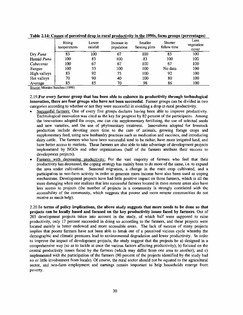
15. Apart from providing the above results, chapter II briefly reviews a study suggesting that ruralproductivity has been declining in the Altiplano in the 1990s. Using focus groups (123 groups in 40communities) and expert interviews with key informants, Morales Sanchez (1999) analyzes theperceptions of farm households in the Altiplano on rural productivity. Overall, the participants in four ofevery five groups indicate that crop yields and livestock productivity have been decreasing over the lastten years. Farmers also say that they have to put in more labor today than ten years ago in order to makea living. The farmers cite a number of climatic, demographic, and environmental factors as being at thesource of their difficulties. A large majority of focus groups (if not all of them) suggest that temperatureshave been rising and rainfall decreasing. Together with the demographic pressure yielding smallerfarming plots, these climatic factors have forced farmers to shorter fallow time, and in turn, the need toraise agriculture production has led to less vegetation cover. For every farmer group that has been able toenhance its productivity through technological innovation, there are four groups who have not beensuccessful. Successful farmers tend to be richer, have more irrigated land, and have better access tomarkets. These farmers are also able to take advantage of development projects implemented by NGO,and they cite technological innovation as the key for their progress. For the vast majority of farmers whofeel that their productivity has decreased, the coping strategy has mainly been to do more of the same, i.e.to expand the area under cultivation. Seasonal migration, a change in the main crop cultivated, and aparticipation in non-farm activity in order to generate more income have also been used as copingmechanisms. Development projects have had little positive impact on those farmers, which is all the moredamaging when one realizes that less successful farmers located in more remote areas also have less

ix

access to projects (the number of projects in a community is strongly correlated with the accessibiliiy ofthe community, which suggests that poorer and more remote communities do not receive as much help).

16. In terms of policy implications, the above study suggests that more needs to be done so thatprojects can be locally based and focused on the key productivity issues faced by farmers. Out of265 development projects taken into account in the study, only 17 percent helped in raising farmerproductivity according to the farmers, and these projects were located mainly in better endowed and moreaccessible areas. The lack of success of many projects implies that poorer farmers have not been able tobreak out of a perceived vicious cycle whereby the demographic and climatic pressures lead toenvironmental degradation and lower productivity. In order to improve the impact of developmentprojects, the study suggest that the projects be a) designed in a comprehensive way (so as to tackle at oncethe various factors affecting productivity); b) focused on the central productivity issues faced by thefarmers (which may differ from one area to another); and c) implemented with the participation of thefarmers (90 percent of the projects identified by the study had no or little involvement from locals). Ofcourse, the rural sector should not be equated to the agricultural sector, and non-farm employment andearnings remain important to help households emerge from poverty.

CHAPTER m: NON-MONETARY INDICATORS HAVE IMPROVED MORE THAN INCOME POVERTY

17. A first non-monetary indicator of well-being is Bolivia's index of unsatisfied basic needs.Bolivia's method for measuring unsatisfied basic needs (Necesidades Basicas Insatisfechas, NBIhereafter) is described in the 1993 Mapa de Pobreza:Una Guia para la Accion Social (Republica deBolivia, 1993; see also INE-UDAPE-CENSO 2001, 2002 for the update based on the 2001 Census). TheNBI is computed as the average of four separate sub-indices for housing, sanitation, education, andhealth. The index for housing is a straight average of sub-indices for the quality of housing materials andthe extent of crowding. The quality of housing materials is itself a straight average of separate indicescomputed for floors, walls, and the roof. The index for basic infrastructure services is the straight averageof sub-indices for sanitation and energy. The sub-index for sanitation is itself a straight average of sub-indices for water and sanitation, and similarly; the sub-index for energy is a straight average of sub-indices for access to electricity and the cooking fuel used by the household. The index for education is thestraight average at the household level of each individual's educational lag. The educational lag for eachindividual is one minus the educational attainment for the individual, which itself depends on theindividual's number of years of schooling, whether or not the individual attends school, and whether ornot the individual is literate. The index for health is one minus a variable that measures whether thehousehold has access to health services, and if it does, to what type of services the household relies on.The overall NBI (straight average of the indices for housing, basic services, education, and health) is usedto estimate poverty by considering as poor all households with a NBI index value above 0.1.

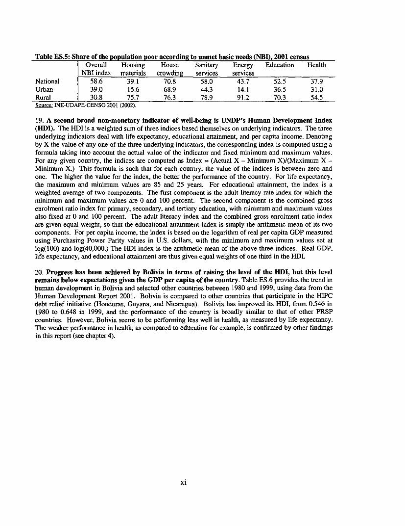
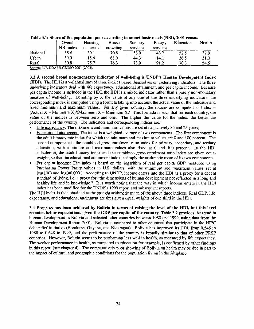
18. In Bolivia as in many other Latin American countries, more progress has been achievedtowards meeting unsatisfied basic needs than towards reducing poverty. From 1976 to 1992, it wasfound that the NBI-based share of poor households in the total number of households decreased from85..5 percent to 70.9 percent nationally. From 1992 to 2001, this share decreased further to 58.6 percent.In urban areas, over the last decade the NBI-based headcount index decreased from 53.1 percent to 35.0percent, but in rural areas, it decreased only from 95.3 to 90.8 percent. Thus while progress has beenachieved since 1992, this has taken place mainly in urban areas, while the needs (and the cost of fulfillingthese needs) are larger in rural areas. Education and health are the areas that improved the most. Sanitaryand energy services follow. Less progress has probably been achieved for housing, but this was to beexpected since this area is less subject to direct Government intervention.

x

Table ES.5: -Share of the population poor according to unmet basic needs (NBI), 2001 censusOverall Housing House Sanitary Energy Education Health

NBI index materials crowding services servicesNational 58.6 39.1 70.8 58.0 43.7 52.5 37.9Urban 39.0 15.6 68.9 44.3 14.1 36.5 31.0Rural 30.8 75.7 76.3 78.9 91.2 70.3 54.5Source: INE-UDAPE-CENSO 2001 (2002).

19. A second broad non-monetary indicator of well-being is UNDP's Human Development Index(HDI). The HDI is a weighted sum of three indices based themselves on underlying indicators. The threeunderlying indicators deal with life expectancy, educational attainment, and per capita income. Denotingby X the value of any one of the three underlying indicators, the corresponding index is computed using aformula taking into account the actual value of the indicator and fixed minimum and maximum values.For any given country, the indices are computed as Index = (Actual X - Minimum X)/(Maximum X -Minimum X.) This formula is such that for each country, the value of the indices is between zero andone. The higher the value for the index, the better the performance of the country. For life expectancy,the maximum and minimum values are 85 and 25 years. For educational attainment, the index is aweighted average of two components. The first component is the adult literacy rate index for which theminimum and maximum values are 0 and 100 percent. The second component is the combined grossenrolment ratio index for primary, secondary, and tertiary education, with minimum and maximum valuesalso fixed at 0 and 100 percent. The adult literacy index and the combined gross enrolment ratio indexare given equal weight, so that the educational attainment index is simply the arithmetic mean of its twocomponents. For per capita income, the index is based on the logarithm of real per capita GDP measuredusing Purchasing Power Parity values in U.S. dollars, with the minimum and maximum values set atlog(100) and log(40,000.) The HDI index is the arithmetic mean of the above three indices. Real GDP,life expectancy, and educational attainment are thus given equal weights of one third in the HDI.

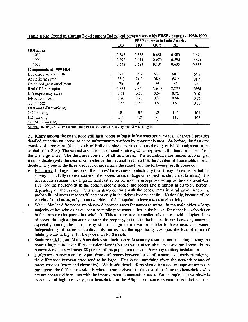
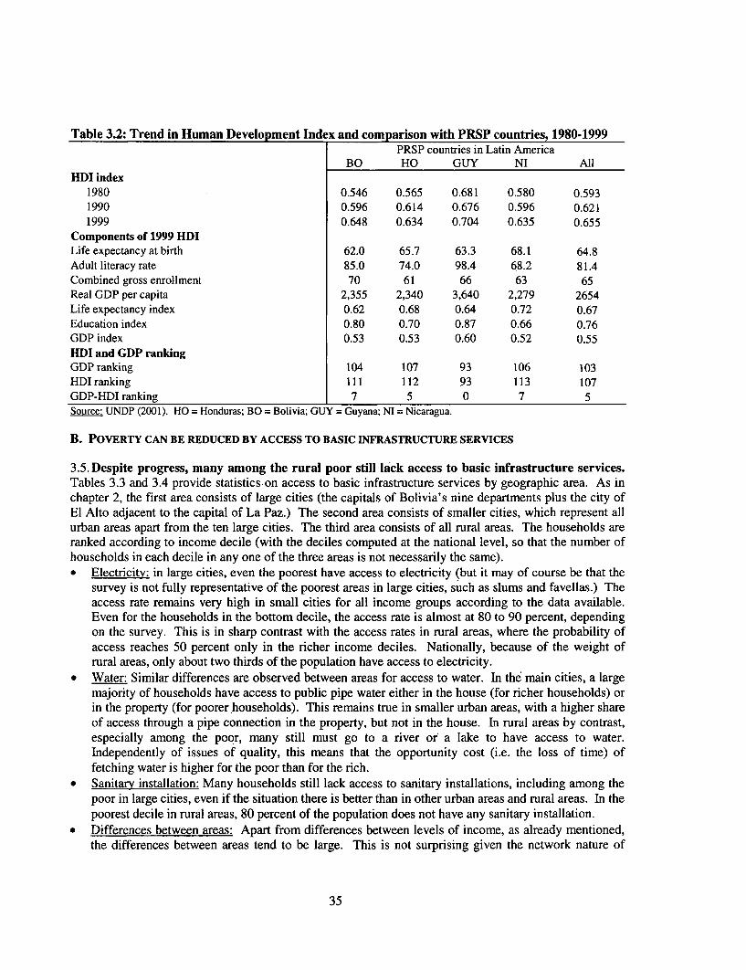
20. Progress has been achieved by Bolivia in terms of raising the level of the HDI, but this levelremains below expectations given the GDP per capita of the country. Table ES.6 provides the trend inhuman development in Bolivia and selected other countries between 1980 and 1999, using data from theHuman Development Report 2001. Bolivia is compared to other countries that participate in the HIPCdebt relief initiative (Honduras, Guyana, and Nicaragua). Bolivia has improved its HDI, from 0.546 in1980 to 0.648 in 1999, and the performance of the country is broadly similar to that of other PRSPcountries. However, Bolivia seems to be performing less well in health, as measured by life expectancy.The weaker performance in health, as compared to education for example, is confirmed by other findingsin this report (see chapter 4).

xi

Table ES.6: Trend in Human Development In ex and comparison with PRSP countries, 1980-1999PRSP countries in Latin America

BO HO GUY NI AllHDI index

1980 0.546 0.565 0.681 0.580 0.5931990 0.596 0.614 0.676 0.596 0.6211999 0.648 0.634 0.704 0.635 0.655

Components of 1999 HDILife expectancy at birth 62.0 65.7 63.3 68.1 64.8Adult literacy rate 85.0 74.0 98.4 68.2 81.4Combined gross enrollment 70 61 66 63 65Real GDP per capita 2,355 2,340 3,640 2,279 2654Life expectancy index 0.62 0.68 0.64 0.72 0.67Education index 0.80 0.70 0.87 0.66 0.76GDP index 0.53 0.53 0.60 0.52 0.55HDI and GDP rankingGDP ranking 104 107 93 106 103HDI ranking ll1 112 93 113 107GDP-HDI ranking 7 5 0 7 5Source: UNDP (2001). HO = Honduras; BO = Bolivia; GUY = Guyana; NI = Nicaragua.

21. Many among the rural poor still lack access to basic infrastructure services. Chapter 3 providesdetailed statistics on access to basic infrastructure services by geographic area. As before, the first areaconsists of large cities (the capitals of Bolivia's nine departments plus the city of El Alto adjacent to thecapital of La Paz.) The second area consists of smaller cities, which represent all urban areas apart fromthe ten large cities. The third area consists of all rural areas. The households are ranked according toincome decile (with the deciles computed at the national level, so that the number of households in eachdecile in any one of the three areas is not necessarily the same), and the following results come out:* Electricity: In large cities, even the poorest have access to electricity (but it may of course be that the

survey is not fully representative of the poorest areas in large cities, such as slums and favellas.) Theaccess rate remains very high in small cities for all income groups according to the data available.Even for the households in the bottom income decile, the access rate is almost at 80 to 90 percent,depending on the survey. This is in sharp contrast with the access rates in rural areas, where theprobability of access reaches 50 percent only in the richest income deciles. Nationally, because of theweight of rural areas, only about two thirds of the population have access to electricity.

* Water: Similar differences are observed between areas for access to water. In the main cities, a largemajority of households have access to public pipe water either in the house (for richer households) orin the property (for poorer households). This remains true in smaller urban areas, with a higher shareof access through a pipe connection in the property, but not in the house. In rural areas by contrast,especially among the poor, many still must go to a river or a lake to have access to water.Independently of issues of quality, this means that the opportunity cost (i.e. the loss of time) offetching water is higher for the poor than for the rich.

* Sanitary installation: Many households still lack access to sanitary installations, including among thepoor in large cities, even if the situation there is better than in other urban areas and rural areas. In thepoorest decile in rural areas, 80 percent of the population does not have any sanitary installation.

* Differences between areas: Apart from differences between levels of income, as already mentioned,the differences between areas tend to be large. This is not surprising given the network nature ofmany services (water and electricity). While additional efforts should be made to improve access inrural areas, the difficult question is where to stop, given that the cost of reaching the households whoare not connected increases with the improvement in connection rates. For example, is it worthwhileto connect at high cost very poor households in the Altiplano to some service, or is it better to let

xii

forces such as migration help in solving the issue over time? These issues are difficult to analyze, butthere is no doubt that they deserve additional analytical work.

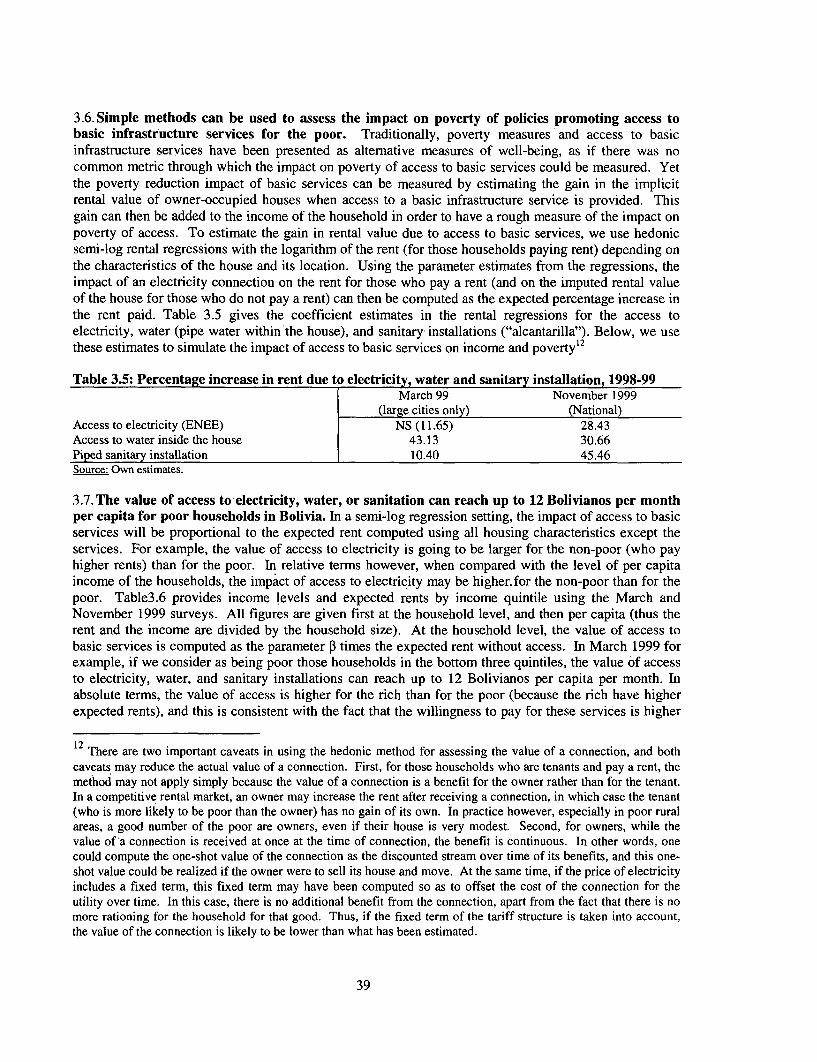
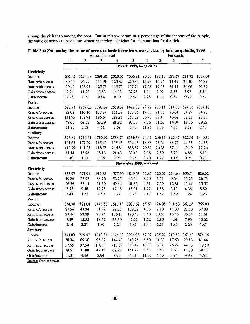
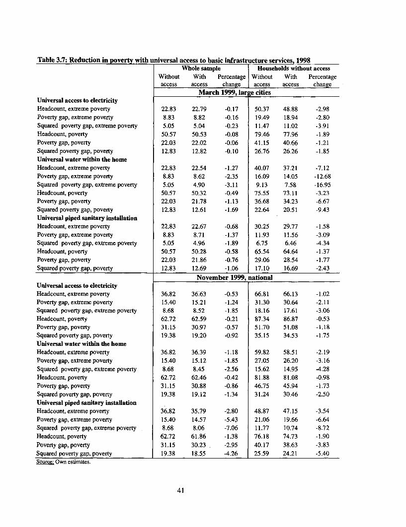
22. Better access to basic infrastructure services has the potential to help for poverty reduction. Thevalue of access to electricity, water, and sanitary installations (as measured through a proxy for thereadiness to pay observed via rents) can reach up to 12 Bolivianos per capita per month for the poor. Inabsolute terms, the value of access is higher for the rich than for the poor, and this is consistent with thefact that the willingness to pay for these services is higher among the rich than among the poor. But inrelative terms, as a percentage of the income of the people, the value of access to basic infrastructureservices is higher for the poor than for the rich. The reduction in poverty obtained when all thosehouseholds who lack access to one of the basic services get access can been computed. In large cities as awhole, if access to electricity is provided to all those who do not have access today, the various measuresof poverty reduction are almost unchanged not so much because the value of the access is not largeenough, but rather because the level of access is already very large in Bolivia's main cities. For water, theestimated reduction in poverty is larger because of a higher value for the connection and also a largershare of household without access within their home. For sanitary installations, we have results falling inbetween those obtained for electricity and water. In smaller urban cities and in rural areas, the potentialfor poverty reduction through better access to basic infrastructure services also tends to be larger.

23. Consultations with the poor emphasize the importance of non-monetary indicators of well-being. As part of a global research project entitled "Consultation with the Poor", a study was conductedin Bolivia in 1999 in order to listen to what the poor have to say about their situation (World Bank,1999a). Employment and other economic issues were considered as important in all the communitiesvisited for the study, but there were differences in emphasis between urban and rural areas. Economicstability was identified with employment in urban areas, while in rural areas economic problems werelooked at more in terms of agricultural production and land issues. Generally, the poor felt that economicconditions have been worsening over time, especially in the Altiplano. While the poor acknowledge theprogress achieved in access to basic infrastructure and social services, they continue in some communitiesto mention these areas as not being satisfactory. When this was the case, urban communities placed moreemphasis on basic services such as water, electricity and sewage, while rural areas emphasizeinfrastructure (roads). Traditional sectors related to human development were not emphasized as much bythe poor as economic issues. This does not mean that the poor do not consider access to, and achievementin education and health as important, but it does suggest that they have more immediate priorities in termsof having a decent standard of living through better employment and agricultural productionopportunities. The emphasis on productive activities can also be interpreted as suggesting that the poor donot want to rely on handouts from the state. Rather, they would prefer to stand on their own feet andemerge from poverty through their work. Personal security also emerged as an important issue, at least inurban areas, where it was closely identified with a lack of well-being. In the urban communities, violenceand delinquency were explicitly identified as problems. In rural areas, the issue of security was broughtup in the context of conflicts over natural resources and worries about diseases. Adult men tended tofocus on economic stability while youth and women emphasized personal security. Many of the poor stillview their communities as safe, but it was felt that insecurity had increased and was deteriorating further.

24. Another finding of the study is that gender roles are changing, women are taking on moreresponsibilities, and domestic violence is decreasing, but all this is happening slowly. In thecommunities visited, the woman is still seen as the main person in charge of caring for the home and thechildren, while the man is seen as the bread winner. If suggested during the conversations, it wasrecognized that women actually work more than men, particularly when they have to combine workoutside the house with domestic chores. Moreover, urban women have been assuming some rolesnormally reserved for men, and single parent households headed by women have also become morecommon. Nevertheless, men remain the main decision makers. While women play a role in making

xiii

decisions regarding the family and "domestic" issues, men are responsible for all "public" decisions. Atthe community level as well, men are expected to make the decisions. Progressively, women are seen ashaving more power now than in the past, and the better education of women is credited for thisevolutions. There is resentment on the part of some men, who see their power to be usurped by women,though other men view this as a general improvement of the community. Usually, domestic violence wasidentified as stemming from men toward women. Abuse from adults toward children was mentioned lessoften. Many women attributed problems of domestic violence and crime to the excessive use of alcohol.But overall, domestic violence was said to be decreasing thanks to changes in attitudes about gender.

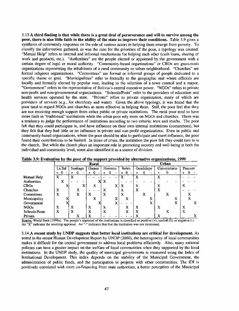
25. A third finding is that while there is a great deal of perseverance and *ill to survive among thepoor, there is also little faith in the ability of the state to improve their conditions. The poor regardNGOs and churches as being more effective than the Government in helping them, but they still feel thatthey are not receiving enough support from either public or private institutions. The rural poor tend tohave more faith in traditional institutions while the urban poor rely more on NGOs and churches. Therewas a tendency to judge the performance of institutions according to two criteria: trust and results. Thepoor felt that they could participate in, and have influence on their own internal institutions (committees),but they felt that they had little or no influence in private and non-profit organizations. Even in publicand community-based organizations, where the poor should be able to participate and exert influence, thepoor found their contributions to be limited. In times of crisis, the institution the poor felt they could turnto is the church. But while the church plays an important role in promoting security and well-being atboth the individual and community level, some also identified it as a source of division.

26. Social capital may have an impact for poverty reduction and economic development. Using asurvey conducted in four municipalities (Charagua, Mizque, Tiahuanacu and Vilkla Serrano), Grootaertand Narayan (2000) suggests that while an overall measure of social capital does not have a statisticallysignificant positive impact on household level per capita expenditures in Bolivia, sub-measures such asthe number of memberships and the contributions of households to community organizations do. Thestudy also suggests that the returns to social capital are higher for the poor than for the rich. Social capitalwas also found to have a positive impact on asset accumulation, access to credit, and collective action.Using a survey for the city of El Alto, Gray-Molina et al. (1999) find a negative correlation betweensocial capital and the probability of being poor. The report on Human Development in Bolivia (UNDP,2000) also suggests a positive correlation between the level of institutional development, the existence ofa democratic culture, and the capacity for development at the local level. In the UNDP study, the qualityof municipal governments is measured using the Index of Institutional Development. This index dependson the stability of the Municipal Government, the administration of public funds, and the participation inprojects with other communities. The IDI is positively correlated with more co-financing from stateauthorities, a better perception of the Municipal Government's work, and a better cooperation between theMunicipal Government and other social institutions in the community. These are, in turn, important forlocal economic development. Strengthening Bolivia's institutions should thus be seen as a key element ofany poverty reduction strategy.

CHAPTER IV: PROGRESS HAS BEEN MADE IN EDUCATION AND HEALTH, BUT MORE IS NEEDED

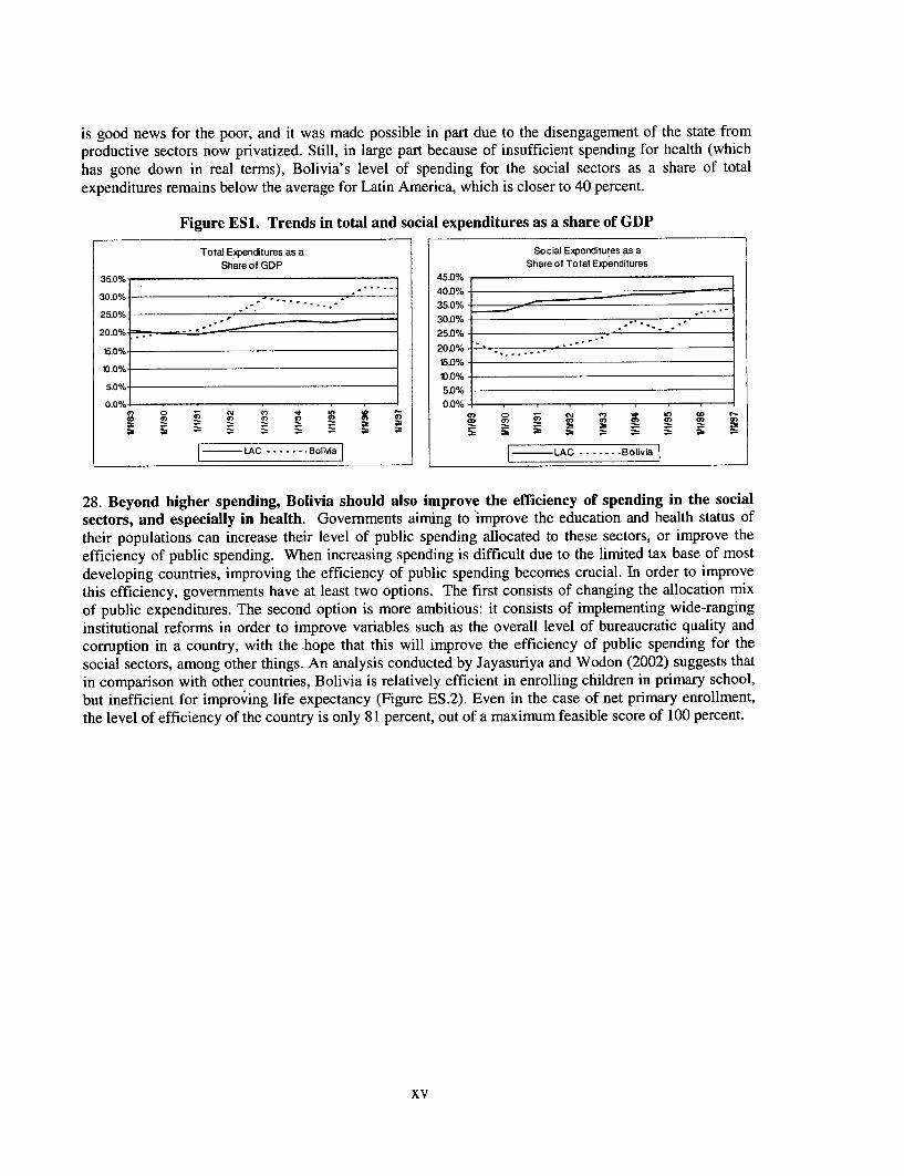
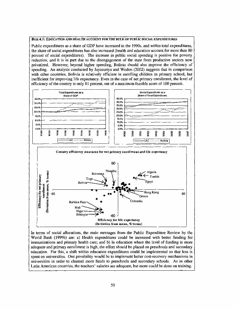
27. Bolivia has made efforts over the last ten years to increase public spending for the socialsectors. The Figures below provides a brief overview of the trend in public social expenditures. Adetailed analysis can be found in the Public Expenditure Review for Bolivia recently completed by theWorld Bank (1999b). According to the IMF's GFS data base, public expenditures in Bolivia increased inthe 1990s as a share of GDP from 20 percent to about 30 percent. Bolivia's growth in public expenditureswas faster than that observed in Latin America as a whole. Within total expenditures, the share of socialexpenditures increased from 20 percent to more than 30 percent. As in other countries, health andeducation account for more than 80 percent of public social expenditures. The increase in social spending

xiv

is good news for the poor, and it was made possible in part due to the disengagement of the state fromproductive sectors now privatized. Still, in large part because of insufficient spending for health (whichhas gone down in real terms), Bolivia's level of spending for the social sectors as a share of totalexpenditures remains below the average for Latin America, which is closer to 40 percent.

Figure ESI. Trends in total and social expenditures as a share of GDP

Total Expenditures as a Social Expenditures as a

Share of GDP Share of Total Expenditures35.0% 45.0%

30.0o% ,, 40.0%35.0% -

15.0% 20.00%

t.0%1 15.0%5.0%

-.-% . . . . . . 0.0%

cm,0 0 0) C3 Ca _, 0e X1 0) _

to-LAC ..... BolMa LAC ----- Bolivia |

28. Beyond higher spending, Bolivia should also improve the efficiency of spending in the socialsectors, and especially in health. Governments aiming to improve the education and health status oftheir populations can increase their level of public spending allocated to these sectors, or improve theefficiency of public spending. When increasing spending is difficult due to the limited tax base of mostdeveloping countries, improving the efficiency of public spending becomes crucial. In order to improvethis efficiency, governments have at least two options. The first consists of changing the allocation mixof public expenditures. The second option is more ambitious: it consists of implementing wide-ranginginstitutional reforms in order to improve variables such as the overall level of bureaucratic quality andcorruption in a country, with the hope that this will improve the efficiency of public spending for thesocial sectors, among other things. An analysis conducted by Jayasuriya and Wodon (2002) suggests thatin comparison with other countries, Bolivia is relatively efficient in enrolling children in primary school,but inefficient for improving life expectancy (Figure ES.2). Even in the case of net primary enrollment,the level of efficiency of the country is only 81 percent, out of a maximum feasible score of 100 percent.

xv

Figure ES.2: Country efficiency measures for net primary enrollment and life expectancy

60

C Nam bia AlgenaBotswvana i

c \ \ ~~~~~~~~~~~~~44 e Tunisia*; ETsolivia TogD

t' e Bolivia ~~~~~~~~~~~~~~Egypt

c4,0 -60 + * Greer e 60

Burkina Faso

a ~~~~~~~a>3 M~~~~~~Nger

Ethiopia -60

FEciency for life expectancy.(Deviation from mean, % terms)

Source: Jayasuriya and Wodon (2002)

29. Substantial progress has been achieved in education, but drop-outs are frequent in the primarycycle and enrollment in secondary school remains low. Enrollment rates in the primary and secondarylevels have improved substantially in the 1990s (Table ES.7). Disparities in education enrollment patternsby gender have also been reduced. Today, while nationally there is still a small difference in schoolenrollment between boys and girls, this is mainly due to small urban areas and rural areas. In departmentcapitals and El Alto, there is no more statistically significant difference in enrollment by gender. Still,while Bolivia's gross enrollment rate is well above 100 percent in primary schools, it is much lower insecondary schools. Drop-out rates remain high, and there remain pockets of low primary schoolenrollment. Recent research also suggests that late entry is an important component of educationalproblems in Bolivia (Urquiola, 2001b). In urban and rural areas, a significant percentage of 6 and 7 year-olds do not attend school, and these children will later on be prime candidates for dropping . Making surethat children do enter school at the right age may be key in terms of raising educational attainment, and itsuggests a role for pre-school and Early Child Development interventions.

Table ES.7: Education Sector Indicators--Pri ary and Secondary Levels, 1990-971990 1993 1996 1997

Coverage (in percent) 76.9 81.9 86.5 87.3Drop-out rate (in percent) 7.2 14.0 9.8 9.8

Retention rate (in percent) 28.7 41.1 45.6 46.2Source: Govemment of Bolivia

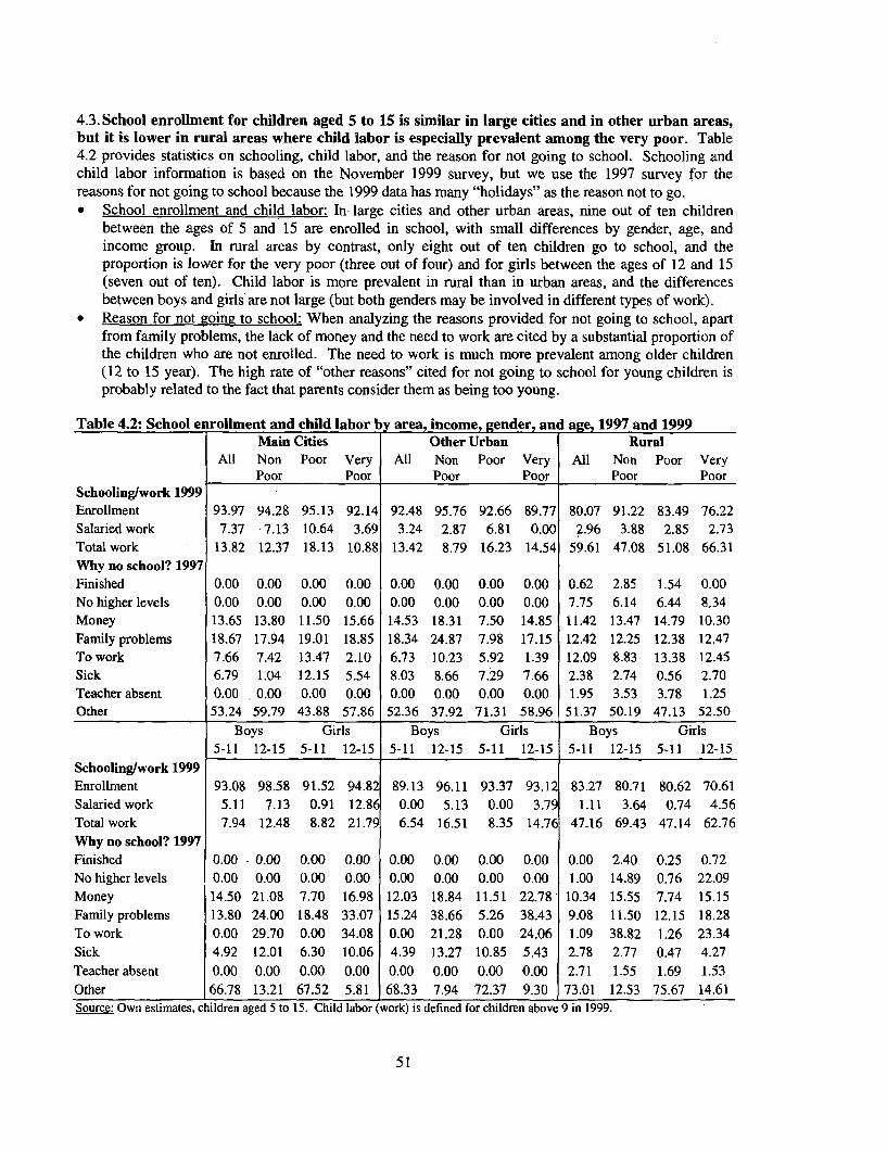
30. School enrollment for children aged 5 to 15 is similar in large cities and in other urban areas,but it is lower in rural areas where child labor is prevalent among the poor. Chapter 4 providesstatistics on schooling, child labor, and the reason for not going to school. In large cities and other urbanareas, nine out of ten children between the ages of 5 and 15 are enrolled in school, with small differencesby gender, age, and income group. In rural areas, only eight out of ten children go to school, and theproportion is lower for the very poor (three out of four) and for girls between the ages of 12 and 15 (sevenout of ten). Child labor is more prevalent in rural than in urban areas, and the differences between boysand girls are not large (but both genders may be involved in different types of work). When analyzing the

xvi

reasons provided for not going to school, apart from family problems, the lack of money and the need towork are cited by a substantial proportion of the children who are not enrolled. The need to work is muchmore prevalent among older children (12 to 15 year). The high rate of "other reasons" cited for not goingto school for young children is probably related to the fact that parents consider them as being too young.

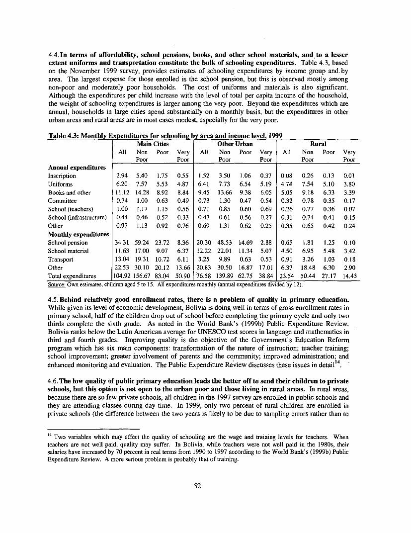
31. In terms of affordability, school pensions, books, and other school materials, and to a lesserextent uniforms and transportation constitute the bulk of schooling expenditures. The largestexpense for those enrolled is the school pension, but this is observed mostly among non-poor andmoderately poor households. The cost of uniforms and materials is also significant. Although theexpenditures per child increase with the level of total per capita income of the household, the weight ofschooling expenditures is larger among the very poor. Beyond the expenditures which are annual,households in large cities spend substantially on a monthly basis, but the expenditures in other urbanareas and rural areas are in most cases modest, especially for the very poor.

32. Beyond relatively good enrollment rates, there is a problem of quality in primary education.While given its level of economic development, Bolivia is doing well in terms of gross enrollment rates inprimary school, half of the children drop out of school before completing the primary cycle and only twothirds complete the sixth grade. As noted in the World Bank's (1999b) Public Expenditure Review,Bolivia ranks below the Latin American average for UNESCO test scores in language and mathematics inthird and fourth grades. Improving quality is the objective of the Government's Education Reformprogram which has six main components: transformation of the nature of instruction; teacher training;school improvement; greater involvement of parents and the community; improved administration; andenhanced monitoring and evaluation. For the teachers, two variables which may affect the quality ofschooling are the wage and training levels. When teachers are not well paid, quality may suffer. InBolivia, while teachers were not well paid in the 1980s, their salaries have increased by 70 percent in realterms from 1990 to 1997. A more serious problem may be that of training. The low quality of publicprimary education leads the better off to send their children to private schools, but this option is not opento the urban poor and those living in rural areas.

33. The supply and quality of Government pre-schools has a positive impact on overall enrollmentin pre-schools. Parents may be unwilling to allow their five to six year old children to travel longdistances to attend preschools, especially since preschools are not prerequisites for primary schools.Given that enrollment is far from being universal in pre-schools, we would expect the supply of pre-schools to have a positive impact on enrollment. The density of Government pre-schools per squarekilometer indeed has a significant impact on participation rates. A one standard deviation increase in thedensity of Government schools (0.043) from the mean density leads to a 4.167 percent increase inparticipation rates. By contrast, the density of private schools is not a significant determinant ofparticipation rates. As for school quality, the ratio of Government school teachers to pupils also has asignificant impact on participation rates, with a one standard deviation increase in the number of teachersper pupil in Government schools (0.054) from the mean leading to a 3.5 percent increase in participation.Again, pupil-teacher ratios in private schools do not appear to have the same impact. Given that inGovernment schools, a teacher is assigned to twenty pupils, versus ten in private schools, it may be thepupil-teacher ratios in private schools is already close to the desirable level, so that changing the ratio atthe margin does not have a significant impact on participation rates. As for the fact that the number ofteachers in Government schools has a positive impact on enrollment, it need not suggest an overallincrease in the number of teachers, since alternatives such as changes in the regional distribution ofteachers may be more appropriate (more work is needed before advocating specific options). Othervariables yielding an increase in participation rates in preschools are the municipality's education level(measured by literacy rates) and its wealth (captured by the number of financial institutions per capita)Geographic and demographic effects are also significant.

xvii

34. The supply and quality of primary and secondary schools do not affect primary enrollmentrates very much, but an increase in pre-school enrollment does yield higher primary enrollment,and higher primary enrollment leads to higher secondary enrollment. Given that enrollment inprimary-school is relatively high in Bolivia, and that the supply is well developed, it is not clear a prioriwhether increasing the supply of schools and their quality would boost enrollment. It turns out that thesupply and quality of Government schools do not affect enrollment at the margin much. The same isobserved at the secondary level, which is a bit surprising. On the other hand, higher preschoolparticipation rates yield higher primary school participation rates, with an increase of one standarddeviation (0.286) in preschool enrollment leading to a one percent increase in primary school enrollment.And higher enrollment rates in primary school also increase enrollment in secondary schools, with anincrease of one standard deviation (0.437) in the primary participation rate from the mean leading to a1.376 percent increase in secondary school enrollment. The policy implication is that investments in pre-schools may be effective in increasing secondary school enrollment through their impact on' primaryschool enrollment. While enrollment rates in pre-schools have increased in Bolivia, only one out of sixchildren below the age of six received early education in 1998. According to the World Bank (1999c),this is below the 1992 Latin American average of 17 percent for children under 5. Pre-schools may alsoyield health benefits such as a decrease in malnutrition rates and child labor. When young children aretaken care of in pre-schools, older siblings are freed to go to school, and mothers can take on productiveactivities or other tasks.

35. Other studies also suggest that pre-schools have positive anthropometric and academic impacts.Bolivia's PIDI (Proyecto Integral de Dessarollo Infantil, now part of the Programma Nacional deAtencion a Ninos y Ninas Menores de Seis Anos) has been recently evaluated by Todd et al. (2000). Theprogram is targeted to poor areas where it provides day-care, nutrition, ands educational services tochildren aged six months to six years. The program's evaluation suggests that the program is welltargeted and tends to have larger positive impact when the children participate for a longer period of time.Although the program may yield larger anthropometric and academic test achievement gains to childrenfrom better off families, it is cost-effective and it should contribute to long term poverty reduction.

36. To improve quality in primary schools, and to better fund pre-schools and secondary schools,cost-recovery mechanisms could be implemented at the university level. Given the low rate ofgraduation from secondary schools (26 percent), enrollment rates at the university level are very high inBolivia (22 percent) and at or above the Latin American average of 20 percent. As a result, the share ofBolivia's education budget devoted to universities is very high, and it has increased substantially in the1990s. University spending is highly regressive, with nine out of ten university students coming from thetop three income quintiles, and two out of five coming from the richest quintile. Cost-recoverymechanisms and stricter admission standards could help in reducing public costs and improving quality.

37. The investments in education infrastructure of Bolivia's social investment funds (SIF) do notappear to have generated large gains in enrolment, attendance, and achievement. According to arecent evaluation by Newman et al. (2002), the SEF interventions have improved Bolivia's educationalinfrastructure, but this did not translate into higher enrollment, higher attendance, and higher achievementrates. One of the only variable showing some progress due to SEF interventions was the drop-out rate.The finding of a lack of impact of SIF on outcomes was robust to the use of alternative methodologiesand regression specifications. The results confirm our finding above that better infrastructure at theprimary (and secondary) levels is not sufficient to improve outcomes, including enrollment. The Ministryof Education is now implementing changes in the projects financed by the SIF in order to place theprovision of better education infrastructure in the context of a better overall intervention package.

38. One of the reasons why poor children do not go to school enough is child labor. There are atleast three problems with child labor. A first problem with child labor is that many children working may

xviii

be at risk of being hurt. Children employed in agriculture, mining, and many other activities are exposedto at least some level of risk. Second, among working children, "street children" face very hard livingconditions. The third and more widespread problem is that by child labor reduces the probability ofschooling, thereby perpetuating poverty from one generation to the next. Given that the children haveonly a given number of hours per day for schooling, labor, and leisure, child labor may lead to lessschooling. When this is the case, the likelihood that the child will emerge from poverty when he reachesadulthood will be reduced since the human capital of the child is reduced. It turns out that the probabilityof going to school when doing paid work varies from 19 percent to 74 percent depending on the sample(urban boys, urban girls, rural boys, and rural girls). The probability of going to school when the child isnot working is much higher, ranging from 64 percent to 97 percent. The difference in the probabilities ofgoing to school when the child is not working, and when the child is working, provides an estimate of thesubstitution effect between work and schooling. The estimates vary from 24 percent to 45 percentdepending on the sample. These results suggest that while substitution effects between paid child laborand schooling are not unitary (child labor can take place after schooling, or the parents can reduce thetime allocated to leisure when children work), they are nevertheless large.

39. Although the cost of child labor seems lower in Bolivia than in other countries, it remainssubstantial. To assess the impact of child labor on children, one can predict future earnings according tovarious levels of education. The assumption is that if a child is working, and if this does not enable himto go to school, the child completes only the primary level of education (six years of schooling, up to age12.) In contrast, if the child is not working, and if this enables him to go to school, the child completesthe lower secondary level (9 years of schooling.) Thus, in the first three years after the completion ofprimary school, a working child enjoys a benefit because he receives a wage. But for the rest of thechild's life, the earnings are lower because of the lower level of education achieved. Computing the netactualized value (with a five percent discount rate) of the difference in the future streams of income withonly primary education, and with 3 years of secondary education provides the cost of child labor in termsof foregone future earnings. The cost is smaller than in Bolivia than in other countries (Siaens andWodon, 2002a), but still significant at 3 to 29 percent of lifetime earnings depending on the sample. Thecost in percentage terms is larger for girls because of the impact of education on the probability to work.

40. Bolivia's performance in the health sector has been poorer than in the education sector. Despitesome progress in the 1990s, Table ES.8 indicates that infant mortality rates and immunization levels (forDPT3, measles, and polio) remain among the worst in Latin America. According to the Demographicsand Health Surveys (DHS), only half of the children receive a vaccine against measles, and theimmunization rates for DPT3 and polio remain below fifty percent. However, Govemment data onimmunization campaign as well as data from the income expenditure survey suggest better coverage (seetable ES.9 for the 1999 income and expenditure survey). As shown in table ES.8, fertility rates aredeclining in part thanks to an increasing usage of contraceptives, but rural areas are still lagging behind.Although the usage of medical personnel and facilities for treatment has increased in the last ten years, itremains low, especially in the case of severe diarrhea. The rural poor are much also much less likely thanthe urban poor to benefit from the assistance of a doctor or a nurse when delivering (not shown in thetable). Almost half of all rural deliveries among the very poor in rural areas takes place with theassistance of family members only. This probably contributes to high infant mortality rates.

xix

Table ES.8: Selected Health Indicators, 1989-19981989 1994 1998

Infant and maternal mortalityInfant Mortality Rate (per 1,000) 96 75 67Under Five Mortality Rate (per 1,000) 130 116 92Maternal Mortality Rate (per 100,000 births) 416 390 NAFertility and contraceptionGross Fertility Rate (Births per woman) 5.6 4.8 4.2Vaccination rates for childrenDPT3 28.3 42.8 48.6Measles 57.5 55.7 50.8Polio 37.8 47.5 39.1Access to and usage of medical personnelPercent of births with some prenatal care by trained medical personnel 44 49.5 65.1Percent of births occurring in medical facilities 37.6 42.3 52.9Percent of Acute Respiratory Infections treated by medical personnel 28.7 43.4 NAPercent of severe diarrhea cases treated by medical personnel 24 32.4 36.4Source: World Bank, based on DHS surveys.

Table ES.9: Alternative estimates of vaccination rates by area and income group, 1999Main cities Small cities Rural

All Non Poor Very All Non Poor Very All Non Poor Verypoor Poor poor Poor poor Poor

First vaccination 90.37 94.76 91.96 82.32 91.88 98.00 95.28 83.68 86.77 82.95 84.21 88.32Second vaccination 75.09 84.94 70.82 65.32 64.82 77.93 61.76 60.04 66.82 59.43 67.24 68.12Source: Own estimates.

41. Malnutrition rates among children under five years of age have improved in the 1990s, but theyremain high among the poor and in rural areas. Malnutrition takes hold during the first two to threeyears of life, but the damage to the immune system, physical growth, and mental development may beirreversible and lead to lifelong handicaps in learning, disease resistance, reproduction, and workcapacity. For example, children who were malnourished at a young age may not be able to learn as wellin school. The incidence of stunting (measured as the share of children below three years of age having aheight at least two standard errors below international standards for that age) has decreased in the 1990s(table ES.10). But stunting remains highly prevalent among poor children (as classified by wealthquintile). Data for 1994 suggest that indigenous children are twice as likely to be malnourished as non-indigenous children. Some progress has been achieved. Iodine deficiency has been virtually eliminatedthrough iodization of salt and proper enforcement. Anemia has also been reduced through an integratedanemia control program (fortification of flour and iron supplementation of pregnant women and childrenunder two years of age). Still, iron deficiency anemia remains widespread since according to the 1998Demographic and health Survey (DHS), with two-thirds of the children under 3 being anemic. This rateincreases to 75 percent for children between 6 and 11 months of age. Vitamin A deficiency is also aproblem, causing immune deficiency (trend data are not available for micro-nutrient deficiencies).

Table ES.10: Child malnutrition by wealth quintile and area, 1994 and 1998Urban Rural

Lowest 2nd 3rd 4th 5th Lowest 2nd 3rd 4"t 5th% children under 3 stunted, 1994 NR 23.5 25.3 18.3 14.0 41.1 32.8 25.4 23.8 NR% children under 3 stunted, 1998 33.7 31.5 22.3 10.8 5.6 39.7 27.3 22.1 17.7 NRSource: World Bank data and Gwatkin et al. (2000). NR means that the data is not representative enough.

42. Despite important financial resources devoted to nutrition in Bolivia, the performance ofnutrition programs is weak. Substantial resources were spent on nutrition programs in 1999 in Bolivia.

xx

Under good targeting and management, this should be enough to help the 186,000 malnourished childrenunder three. Unfortunately, malnutrition money is not being spent well enough. Targeting is not verygood, with only 8 percent of the resources are devoted to cost-effective interventions targeted to childrenunder two and pregnant women. There are excessive concerns with food supply, particularly anoveremphasis on animal products, to the detriment of an action on disease and behavioral causes ofmalnutrition. That is, nutrition programs consist essentially of food handouts, and little is done in termsof communication for behavior change. Nutrition programs also lack adequate planning, implementation,and evaluation mechanisms. But perhaps the most serious constraint to improving nutrition is the lack ofpriority or sense of urgency to addressing the problem of malnutrition. Because poverty alleviation byitself is unlikely to improve nutrition quickly, better direct interventions are needed. These need not becostly. Even at their current level of income, the poor could have better nourished children if theychanged their feeding practices so as (for example) not to rely exclusively on breastfeeding in the first sixmonths of age, promote the dietary management of diarrhea, and increasing the variety of foods served tochildren.

43. Affordability remains a barrier to the demand for health care among the poor. In a number ofcases, the very poor spend as much as the moderate poor and the non-poor for health care. This suggeststhat health expenditures are much more of a burden for the very poor (and the poor) than the non-poor.To deal with this situation, the Government introduced a Basic Health Insurance Program with municipalparticipation in order to provide basic care (Seguro Basico). Preliminary evaluation results suggestpositive outcomes in terms of coverage, but also management problems. Also, while adults among thevery poor do not appear to have a higher probability of being sick or injured than the moderate poor andthe non-poor, the probability that they will not seek a consultation when sick or injured is larger. Thereasons why many of the very poor do not seek consultation when sick or injured have mainly to do witha lack of financial resources, at least in large and small cities. Not surprisingly, the very poor are lesslikely than the moderate poor and the non-poor to seek and receive treatment in hospitals and privateclinics when sick or injured, and they are as likely (but proportionately more likely if one excludes thoseamong the very poor not seeking treatment) to use health centers and health posts. The distance to healthfacilities in rural areas is larger. Finally, even though some services are supposed to be free, the poor stilloften pay informally (Chakraborty et al., 2002). This may contribute to lower rates of consultation.

44. One of the reasons for the lack of usage by the very poor of health care facilities and for highhealth care private expenditures is that public expenditures in the health sector are too low. Asdocumented in the Public Expenditure Review of the World Bank (1999b), health expenditures in realterms have been declining in Bolivia, despite already low levels in the early 1990s. Due to thedecentralization, the share of public health expenditures attributed to the Ministry of Health has been cutin half, and the cut has not been compensated by a corresponding increase at the municipal level.Administrative costs within the Ministry of Health have increased, and a large share of health budget isallocated to War of Chaco veterans which ended over 60 years ago. After administrative costs and theallocation to Veterans, what remains available for medicines, vaccines, and maintenance is too low.

45. The World Bank's Public Expenditure Review discusses issues related to the organization of thehealth sector. The Public Expenditure Review (World Bank, 1999b) suggests that in the context of thedecentralization, the Government should simplify and make more explicit the responsibilities of thevarious levels of intervention (national, prefecture, municipal) in the delivery of health services. The co-financing by the central government of local health projects could be based on the positive externalitiesinvolved in the projects. The Government must also exercise leadership in ensuring that the funds madeavailable by donors are put to the best use from the point of view of the country, and that the country hasthe capacity to take over the projects externally financed when support is terminated. The report suggeststhat the country needs more medical personnel and less administrative employees in the health system,and more nurses in comparison with the number of doctors. Finally, while medical professions were not

xxi

well paid in the 1980s, substantial raises in real terms have been allocated in the 1990s (plus 62 percentbetween 1991 and 1997). As is the case for teachers, the compensation level is less of a problem today.

46. Contrary to what was observed in the case of education, the investments in health of the socialinvestment funds appear to have generated significant gains in health outcomes. The evaluation ofthe SIF by Newman et al. (2002) suggests that child mortality has been reduced by SIF interventions.One hypothesis is that SIF investments improved the likelihood of prenatal control, which in turn reducedchild mortality. This was confirmed by the data within SIF areas, in that the reduction in mortality waslarger among those who used the clinics for prenatal control than among those who did not. Thereduction in child mortality is less likely to be due to SEF water investments since there is no evidencethat the quality of the water improved as a result of these investments.

CHAPTER V: GROWTH IMPROVES MONETARY AND NON-MONETARY INDICATORS OF WELL-BEING

47. In part thanks to the implementation of structural reforms, Bolivia's economic growthimproved after the mid 1980s, but there has been a slow down in recent years. Bolivia was one ofthe first Latin American countries to implement structural adjustment policies and wide-ranging reforms.A new economic policy was announced by the Government in August 1985 with the support ofdevelopment agencies. Hyperinflation was brought under control, the deficit of the public sector as ashare of GDP was reduced, and growth resumed. Structural reforms adopted in the 1990s include broad-based liberalization for prices, interest rates, exchange rates, and trade. They also include theprivatization of state owned enterprises, pension reform, as well as judicial and administrative reform.These reforms have not solved all problems, but they are likely to have contributed to growth. Easterly etal. (1997) estimate that the reforms implemented between 1986 and 1990 boosted annual growth by 1.6 to3.3 percent in 1991-93. For 1990-98, GDP grew at an average of 4.2 percent per year (3.7 percent inLatin America). With a population growth rate of 2.4 percent, this translates into a growth in per capitaGDP of 1.8 percent per year. Yet the growth performance of the country has deteriorated in recent years.

48. Although there should be a focus on the impact of growth on poverty rather than onredistribution, this does not mean that growth should be promoted independently of redistribution.In a country like Bolivia where there is not that much to redistribute, and where more than half of thepopulation is poor so that whatever is redistributed must be shared among many, growth should be thepreferred engine of poverty reduction. Yet the priority that we give to growth as opposed to redistributiondoes not mean that redistribution does not matter. For any given level of income and growth,redistribution has the potential to alleviate poverty. Perhaps more importantly, apart from the directimpact that a reduction of inequality has on poverty, two arguments can be made for advocatingredistribution in order to increase the rate of growth. First, higher initial inequality may result in lowersubsequent growth, and thereby in lower poverty reduction over time. This is in part because under highinequality, access to credit and other resources is concentrated in the hands of the privileged, therebypreventing the poor to invest or protect themselves from shocks. Second, higher levels of inequalityreduce the benefits from growth for the poor. This is because a higher initial inequality reduces the shareof the gains from growth that goes to the poor. At the extreme, if a single person has all the resources,then whatever the growth, poverty will never be reduced through growth. In other words, a high level ofinequality may reduce (in absolute terms) the elasticity of poverty reduction to growth. These argumentssuggest that instead of hampering growth, well designed redistributive policies may promote growth andincrease the benefits from growth.

49. In urban areas, a one percentage point increase in per capita income (i.e. a growth rate of onepercent) reduces the headcounts of poverty and extreme poverty by one third of a point. In ruralareas, the impact on poverty is a bit larger, at up to half a percentage point. The impact of economicgrowth on poverty (and inequality) in Bolivia is similar to that observed in Latin America as a whole. The

xxii

estimates of the elasticity of poverty to growth can be used to simulate future poverty measures. Anillustration is given in table ES. 1. Consider as initial conditions the headcount of extreme poverty inurban areas (both large and small cities) and rural areas in 1999 as given in chapter 1, at respectively23.85 and 58.80 percent. Given the urbanization rate in 1999 of 63.74 percent (this rate differs slightlyfrom the one observed in the surveys), the national headcount for extreme poverty is then 36.52 percent.For poverty, the corresponding figures are 51.51 percent in urban areas, 81.71 percent in rural areas, and62.46 percent nationally. Assuming a growth in per capita income of 2 percent over the period 2000-2015, the headcount index of extreme poverty can be expected to be reduced in urban areas to 19.03percent and in rural areas to 38.58 percent by 2015. Nationally, assuming no change in urbanization,extreme poverty and poverty are reduced to 26.12 and 54.42 percent. Taking into account the increase inurbanization (so that the weights for urban areas and rural areas change over time in the estimation ofnational poverty), extreme poverty is reduced nationally by an additional 2 percentage points, to 24.04percent, and poverty is reduced to 52.01 percent. These simulations are crude, but they give an idea ofthe gains towards poverty reduction that can be expected in the future. To reduce poverty further, thecountry would need to increase either its GDP growth rate or its elasticity of poverty to growth. A tenpercent increase in per capita GDP growth (to 2.2 percentage points per year) would have the sameimpact as a ten percent increase (in absolute terms) in the elasticity of poverty to growth.

Table ES.11: Poverty measures: An hypothetical illustration with growth at 2 percent per capitaWith urbanization W/o urbanization Urbanization and rural and urban poverty (headcount)

National National National National Urbani- Urban Rural Urban Ruralextreme poverty extreme poverty zation rate extreme extreme poverty poverty

Year poverty poverty poverty poverty1999 36.52 62.46 36.52 62.46 63.74 23.85 58.80 51.51 81.712000 35.56 61.41 35.78 61.61 64.41 23.56 57.27 50.60 80.962001 34.63 60.37 35.06 60.77 65.07 23.28 55.78 49.71 80.212002 33.74 59.34 34.36 59.95 65.74 23.00 54.33 48.84 79.482003 32.87 58.32 33.67 59.13 66.40 22.73 52.92 47.98 78.742004 32.03 57.31 33.00 58.33 67.06 22.45 51.54 47.13 78.022005 31.23 56.31 32.34 57.54 67.73 22.18 50.20 46.30 77.302010 27.58 51.47 29.27 53.77 71.05 20.88 44.01 42.37 73.812015 24.51 46.90 26.52 50.27 74.37 19.66 38.58 38.77 70.48

Source: Own estimates.

50. Apart from reducing poverty, growth also improves non-monetary indicators of well-being.Economic growth has positive impacts on a wide range of non-monetary indicators including infantmortality, under five mortality, enrollment in secondary education, illiteracy, access to safe water, and lifeexpectancy. Again, using estimated elasticities of non-monetary indicators to growth, simulations can bedone to see the magnitude of gains which can be expected in the future, also taking into account theimpact of urbanization. Such simulations are discussed in chapter 5, and they can be implemented easilyusing Excel-based simulators known as "SimSIP" (Simulations for Social Indicators and Poverty).

51. Empirical work suggests that the poor may benefit more than the non-poor from an expansionin education services, and less than the non-poor for infrastructure and health services. Whilegrowth improves non-monetary indicators of well-being, it remains to be known whether the poor benefitmore or less than the non-poor from this improvement. It can be suggested that in education, those livingin the bottom third of all municipalities in terms of an index of wealth tend to benefit more from anoverall increase in access to services than those living in middle group or the top third of municipalities.This is the case for pre-schools, primary schools, and libraries (for secondary schools, there are nostatistically significant differences in marginal benefit incidence.) In infrastructure, access to water is theonly service for which those living in the bottom third of municipalities benefit as much from an

xxiii

expansion of the service as those living in the other two groups of municipalities. In all other cases(sewage, electricity, garbage collection, and telephone), the less poor benefit more than the poor from aservice expansion. In health, the benefits from an expansion of the services also tend to favor the lesspoor municipalities. While these differences need not persist over time (once the non-poor have nearuniversal access, the poor benefit the most from any additional provision), they highlight the need toimplement special policies at an early stages for the provision of infrastructure services if the poor are tobenefit from these services.

52. Yet our understanding of the determinants of growth, especially for the poor, remains weak.We still need additional work to better understand the determinants of growth itself, includingimprovements in productivity and competitiveness (a study is being financed by the World Bank on thistopic). We also need to better understand how growth could be more pro-poor, for example with higherbenefits for the productive sectors in which the poor are involved the most. The findings of this report arefairly limited in this area, which should be investigated in subsequent work.

xxiv

CHAPTER I: TREND IN POVERTY AND INEQUALITY

A. THIs REPORT WAS WRITTEN AS A CONTRIBUTION TO THE NATIONAL DIALOGUE II AND THEPRSP

1.1. The report was prepared jointly by staff from the Government of the Republic of Bolivia(GRB) and the World Bank, with input from other development agencies. On the part of the GRB,the report benefited from contributions from staff from the National Statistical Institute (INE, InstitutoNacional de Estadistica) and the Unit for the Analysis of Economic Policies (UDAPE, Unidad deAnalisis de Politicas Econ6micas)'. Inputs for, as well as comments on the report were received fromother Government agencies and donors, including the Inter-American Development Bank (IADBhereafter) and the United Nations' Development Programme (UNDP hereafter). The report was preparedin part to serve as an input for the National Dialogue II which took place in the summer of 2000.

1.2. For the preparation of the National Dialogue II, the focus of the report was placed on adiagnostic of poverty in Bolivia without entering into a debate about policy options. A summaryversion of this report was distributed during the National Dialogue II. The present report is madeavailable in order to provide a more detailed analysis of poverty. Chapter 1 provides trends for povertyand inequality. Chapter 2 discusses the determinants of per capita income, and thereby of poverty andinequality. Chapter 3 is devoted to aggregate non-monetary indicators of well-being, with a focus onbasic infrastructure services. Chapter 4 is devoted to education, nutrition, and health. Chapter 5 assessesthe impact of growth on both monetary and non-monetary indicators of well-being. Apart from givingempirical results and providing reviews of existing work, we provide methodological annexes inAppendix in an effort to make our methodological assumptions clear. It should be emphasized at theoutset that this report covers only a limited number of topics, and that the report does not enter into apolicy debate, even if the analysis provided in the report sometimes directly leads to valuable insights forpolicy.

1.3. Apart from being an analytical contribution for Bolivia's National Dialogue II, this report wasalso used for the Poverty Reduction Strategy Paper prepared by the Government. Bolivia is one offour Latin American countries that are participating in the Highly Indebted and Poor Countries (HIPC)initiative providing debt relief to highly indebted and poor countries worldwide. In order to participate inthe HIPC initiative, as is the case for other countries, the GRB prepared a so-called Poverty ReductionStrategy Paper (PRSP). The PRSP contains a diagnostic of poverty in the country based in large part onthis report, a strategy for its reduction, and a number of targets that can be monitored over time in order toassess the performance of the country in reaching its goals. The strategy was prepared in dialogue withcivil society. The PRSP was written by the GRB, not by the World Bank, the International MonetaryFund, or any other international organization. While the Government wrote and owns the PRSP, and isresponsible for its implementation, international organizations provided technical assistance. Providingsuch assistance was the main objective of this report and of the collaboration that took place between theWorld Bank, INE, and UDAPE for its preparation.

1.4. The success of the Government in improving the well-being of Bolivia's population should bemonitored over time using a battery of indicators rather than poverty measures alone. Bothmonetary and non-monetary indicators have been proposed to assess the impact of government policies.

IIn the process of writing this report, World Bank staff came twice to Bolivia, and a staff member from UDAPEcame to Washington, DC. Under the umbrella of the MECOVI program, close collaboration was also maintainedbetween the World Bank., UDAPE, and the INE for the analysis of the November 1999 survey (see Box 1.2).

1

* Monetarv indicators: Within the realm of monetary indicators, the level of growth in per capitaincome or expenditures is a first measure of the performance of a country in increasing well-being.This can be estimated using National Accounts or nationally representative surveys. Beyond growth,

in order to take into account distribution issues, analysts have used a range of inequality and povertymeasures2. Because computing these measures is difficult (it requires good data, good analysis, andmany methodological assumptions), there is typically a debate in most countries as to the level ofdistribution-sensitive monetary indicators and their trend over time. We do provide levels and trendsfor poverty and inequality in this report, but we believe that there are problems of comparability overtime in the household level data, so that the trends presented here should be considered with caution.Many of the problems we are confronted with in estimating past poverty could be avoided inmonitoring future poverty, provided future surveys are made comparable to the November 1999Encuesta Continua de Hogares - Condiciones de Vida. Box 1.2 explains how some features of thatsurvey should provide a better basis for future poverty and inequality measurement than past surveys.

* Traditional non-monetarv indicators: Many argue that poverty and well-being are multidimensionalphenomenon which are not well represented by monetary measures of well-being only. We agreewith this argument (which does not diminish in any way the need to estimate trends in poverty andinequality), and we therefore analyze several non-monetary indicators of well-being in this report.One well-known indicator is the Human Development Index proposed by the UNDP. Others well-known indicators tend to be specific to sectors such as health (malnutrition, infant mortality, etc.),education (enrollment, assistance, repetition, drop-out, etc.), and basic infrastructure services(electricity, sewerage, sanitary installation, safe water, etc.) Many (but not all) of these otherindicators have been analyzed in Bolivia under the umbrella concept of unmet basic needs. These andother non-monetary indicators of well-being are discussed in chapters 3 to 5.

* Other non-monetary indicators: Traditional monetary and non-monetary indicators still do not fullycapture the level of well-being of a population. For example, while domestic violence within thehousehold and social capital within the community matter, they cannot be analyzed using traditionalmeasurement tools. Subjective perceptions of welfare, and more generally the priorities of the poor,also cannot be revealed with standard tools. In this report, we do not analyze many of these issues in

any depth. But we provide a brief summary in chapter 3 of the results of a qualitative studyconducted by the World Bank (1999a) in Bolivia in order to listen to what the poor have to say. Thestudy placed its emphasis on the perception of poverty among the poor, their priorities, the roleplayed by institutions in their life, and gender relations. Another study on the aspirations of Bolivia'spopulation was done by UNDP (2000) in part using data collected by INE (Box 1.1).

* Monetary conversion of non-monetary indicators: In some cases, it is feasible to put a monetary valueon non-monetary indicators, and this can be useful for the analysis of trade-offs between policies. Inchapter 2, we analyze the income gains from education and employment. In chapter 3, we estimatethe value of having access to basic infrastructure services. In chapter 4, we compute the future loss inincome for children working at a young age. These exercises provide valuable information, but theyneed not capture the full cost or benefit (monetary and non-monetary) of what is observed. Forexample, there is an intrinsic value in being well educated, or in having a good job, which goesbeyond the monetary income provided by education and employment. This has to be kept in mind inorder not to base policy decisions on a monetary cost-benefit analysis only. There is also an intrinsicmerit in having public policies that promote better access of the poor to institutions, including thoserelated to the political process at both the local and national levels. Because the very poor typicallyhave no or little voice, improving the quality of Government institutions and building capacity among

2Another alternative to analyze changes in monetary well-being is to use welfare functions taking into account in aflexible way the full distribution of income or expenditures. While it is standard in a poverty diagnostic to providemeasures of growth, inequality, and poverty, and to analyze the relationships between these concepts, it has not yet

become standard to use welfare functions. We plan to use welfare functions in subsequent work on Bolivia.

2

grass-roots organizations should be an integral part of a poverty reduction strategy. If many of theseissues are not discussed in detail, it due to a lack of time and resources, rather than to of a belief thatthey do not matter. Again, some of these issues are discussed in the recent study by UNDP (2000).

Box 1.1: ASPIRATIONS AND INSTITUTIONS: BOLIVIA'S HUMAN DEVELOPMENT REPORT 2000

In this report, we focus on the traditional concept of poverty in terms of the command of households overgoods and services through income and consumption. Although we analyze non-monetary dimensions ofwell-being, we do not talk in details about the aspirations of the Bolivian population and the country'sinstitutions. Some of these topics are discussed in more details in the recently published HumanDevelopment Report (HDR) for Bolivia by the United Nations Development Program (2000). The HDRattempts to identify and analyze the values and aspirations of the Bolivian people, and it suggestsstrategies to achieve development goals within the diverse social, cultural and economic environment ofBolivia.

The HDR suggests that personal and community aspirations will most likely be attained throughdeliberations whereby these aspirations can be translated into agreements that favor human development.The HDR also suggests that in order to develop, Bolivian society needs to combine a pragmatic logic witha pluralist and participatory logic. These conclusions are based on the following main findings:1. Bolivians share values and aspirations which reinforce republican values, legitimize those that are

democratic, and demand new equity goals for Bolivia's future.2. The viability of a deliberation culture in a democratic society such as Bolivia's is limited by the

effectiveness and efficiency of its institutions and the lack of legitimacy of political actors andinstitutions. Such problems affect the ability to govern and must be addressed as quickly as possible.

3. Bolivian firms are lucid and adamant about national issues but they express doubt with respect totheir own ability as well as the Bolivian society's ability to actually address the problems and solvethem.

4. At the local level, institutional consolidation and the development of political elite groups areeffective means to articulate the people's aspirations through decision-making scenarios that arecloser to their daily lives. Here, local development fostered by the Popular Participation Law is astrategic factor.

5. Bolivian society possesses collective capabilities within territorial areas such as the community, theneighborhood, the family and the work site, that allow it to promote greater human development.However, modernization tends to weaken these links.

6. There are problematic trends in the people's reflexive capacity to manage the complexity of modernlife and in the levels of socialization. Although sociability levels are high, there is distrust in urbanareas. Reflexivity is good among the better off, but it is lacking among the poor who need it most.

7. Social inequalities and poverty are deeply rooted. Poverty is not only an inability to meet basic needs,but also a state of deprivation leading to a lack of participation in the country's political process, andreduced aspirations. Due to a lack of opportunities, fatalism and resignation perpetuate poverty.

8. The role of women and how they perceive themselves has undergone significant changes. Forexample, violence in the home is now clearly rejected by a confluence of different groups of womanand men. However, there are also persistent values and customs in society that inhibit equity ingender relationships, particularly with regard to the role of women in the family.

9. Weak institutional development, social and symbolic inequities, and the absence of equitablecommunication and dialogue among the country's different socio-cultural groups are all obstacles toan effective deliberation culture.

3

Box 1.1: CONTINUED

10. There are hurdles to overcome in order to achieve effective communication and to design actionswhich promote human development. Society's aspirations for equity must be resolved within thetrend towards globalization and a concentration of power and wealth. There are also divergentaspirations between regional and municipal elite groups committed to the transformation process andthose who still foster traditional practices. Finally, sociability is concentrated in a group that belongsto the rural world and has a low socioeconomic level, while reflexive capacity to handle modemcomplexity resides in the urban world, especially among people below 30 who enjoy a highsocioeconomic level.

The above findings on the values, aspirations and barriers to a deliberation culture in the Bolivian societypoint to a potential agenda to foster human development. The HDR suggests:* The coordination of actions between the State and society and the establishment of a lay State which

promotes equity and respect for all cultures and identities;* The creation of deliberation fora with new modalities of collective action and the promotion of an

institutional culture to prevent conflicts;* The development of participatory mechanisms and the promotion of social capital to prevent social

disintegration, among others by decentralizing public management, creating new fora for local urbanmanagement, and supporting institutional innovations stemming from local initiatives;

* The establishment of networks and links among communities, institutions, persons and the State;* The development and strengthening of an active and modem citizenry in order to foster equity, with

special regards to gender relationships;* The promotion by the State of an autonomous long-term cultural project at the public level;* The support by the mass media of the establishment of a public deliberation forum for Bolivians from

different cultures, socioeconomic levels, ages and genders by granting visibility to all groups andpromoting the strengthening of communication skills;

* The improvement of the party representation system to expand representative democracy.

One distinctive characteristics of the report is its reliance on a complex process of data collection. Thereport is based on 25 case studies, 17 workshops offered by experts in regional as well as specializedtopics, 13 focus groups involving elite corporate participants throughout the country, a workshop for themayors of 100 of Bolivia's most impoverished municipalities, two Delphi surveys for municipal elites, abroad bibliographic review, two intemational evaluation workshops, and a national survey with a samplesize of 10,000 persons. This household survey of aspirations is especially rich and interesting, andadditional work could be done relating the aspirations of the population to its income and human assets.

B. THERE HAS BEEN A DECREASE IN POVERTY IN THE 1990S IN LARGE CIT1ES

1.5 The level of poverty in a country is what matters in real life. But it is the trend in poverty, notits level, which matters for the evaluation of public policies. The role of a PRSP is to help a country inreducing not only its rate of poverty, but also the number of its poor which tends to increase withpopulation growth when the rate of poverty is left unchanged. Reducing the level of poverty is the goal.But the measurement of progress towards that goal is the poverty trend, i.e. the change in level over time.It often happens that different analysts find different poverty levels because they use differentmethodologies for measuring poverty. This is not a problem as long as they agree on the trend. Apoverty level is normatively defined, and therefore subjective. For practical purposes, a poverty trend isneither normative, nor subjective: it is a fact. Below, we focus on the trend in poverty, not its level.

4

1.6 Previous studies on poverty in Bolivia have suggested an improvement from the mid 1980s tothe mid 1990s. Our own work goes beyond previous studies in three different ways. In the mid1980s, the GRB implemented sweeping reforms and a new economic policy. Through most of the 1990s,per capita GDP grew at a steady rate, making Bolivia one of the better performing economies in LatinAmerica. Has growth reduced poverty? Due to data limitations (see Box 1.2), most existing studiesfocus on large cities. The studies suggest an improvement over time3. Pereira and Jimenez (1998) find adecrease in the household-based headcount index of urban poverty (the share of the households with percapita income below the poverty line) from 53.3 to 45.1 percent between 1990 and 1994. Vos et al.(1998) suggest a decrease in urban poverty between 1988 and 1995 for a population-based headcount (theshare of the population with per capita income below the poverty line), from 70.8 to 59.3 percent.Jimenez and Yavez (1997) find a decrease in the household-based headcount index of urban povertybetween 1990 and 1995, from 53.3 to 47.8 percent. Gray-Molina et al. (1999) report similar findings forthe same period. In its Panorama Social, CEPAL (1999) indicates that the household-based headcountindex of urban poverty was reduced from 47 to 44 percent between 1990 and 1997. In a study for 12 LatinAmerican countries, Wodon et al. (2000) finds a decrease in the population-based urban headcount from70 to 64 percent between 1986 and 1996. Finally, Hermany Limaniro (1999) finds decreasing urbanpoverty between 1989 and 1997. In this chapter devoted to the trend in poverty and inequality, and in thenext chapter devoted to their determinants, we extend previous work in three ways. First, we update thepoverty trends for Bolivia's main cities with poverty estimates for 1993, 1997, and 1999. Second, weprovide estimates of poverty in smaller cities and in rural areas in 1997 and 1999. Third, apart fromgiving a profile of poverty by household characteristics, we use detailed regressions to analyze thedeterminants of poverty in large cities (department capitals), smaller cities, and rural areas.

3One of the studies which did not suggest an improvement is the poverty assessment for Bolivia by The WorldBank (1996), which indicates an increase in the population-based headcount index from 60.1 percent in 1989 to 61.6percent in 1993, but this may be due to the unique recession in Bolivia in the 1990s which occurred in 1992.

5

Box 1.2. DATA FOR POVERTY MONITORING AND ANALYSIS IN BOLIVIA

This box presents the household surveys used for poverty monitoring and analysis in Bolivia and in thisreport, and the initiatives that have been implemented in order to improve data collection and analysis. Italso outlines briefly how future poverty analysis should be conducted (and could be improved) if thesurvey Encuesta Continua de Hogares - Condiciones de Vida becomes available on a regular basis.

Census data and household surveys used in this report

There are currently two main sources of data used for measuring and monitoring poverty in Bolivia: anational census (of which the latest installment was in 1992) and various household surveys.

The census (Censo Nacional de Poblacion y Vivienda) provides data on non-monetary indicators of well-being. This information is being used for building poverty maps and targeting government interventionsusing the concept of Unmet Basic Needs (Necesidades Bdsicas Insatisfechas). The key reference is theMapa de Pobreza: Una Guia Para la Accion Social (Republica de Bolivia, 1993) which describes themethodology in detail (see chapter 3). An update of Bolivia's NBI-based poverty map was recentlyprepared by INE-UDAPE-Censo 2001 (2002).

Apart from the Census, Bolivia's National Statistical Institute (Instituto Nacional de Estadistica, hereafterINE) has implemented over the years a number of multi-purpose household surveys.

* Up to 1995, INE implemented the Encuesta Integrada de Hogares in Bolivia's main cities. Keyresults for 1989-1995 are available on CD-Rom, and standardized data files for selected years havebeen prepared by CEPAL. In this report, we use mainly the 1993 survey for that period.

* In 1996 and 1997, INE implemented three rounds of the Encuesta Nacional de Empleo (June 1996,November 1996, and November 1997). These surveys have a national coverage. We use the June1996 and November 1997 surveys in this report. The November 1997 survey is the richest in terms ofcontents because it has more detailed modules on education and health.

* In March 1999, INE implemented the Encuesta Continua de Hogares. The coverage is again forBolivia's main cities only. The survey provides information on both income and expenditures,although the expenditures module is a bit short.

* In November 1999, NE implemented the Encuesta Continua de Hogares - Condiciones de Vida. Thecoverage is national. This survey benefited in part from the support of MECOVI (see below). Therange of questions in the survey is more comprehensive than in previous surveys thanks to moduleson health, education, occupation, income, and expenditures. The module on expenditures should beespecially useful for future poverty monitoring.

The fact that all these surveys are not always comparable (for example, there are changes over time in thequestionnaires), and that some of surveys were implemented in large urban areas only, makes it difficultto establish a national trend in poverty in Bolivia in the 1990s. In this report, we do not provide such atrend for the decade as a whole. We limit ourselves to the trend in large cities using surveys for 1993,1997, and 1999, and to the change in poverty in other areas and nationally from 1997 to 1999. Additionalinformation for rural areas is also available thanks to two surveys conducted by Bolivia's social fund(Fondo de Inversion Social, hereafter FIS) in its areas of operations in 1993 and 1997. But these surveysare not fully representative of riral areas, so that results should be treated with caution.

6

Box 1.2: CONTINUED

Improving future poverty analysis

The information in the surveys for the 1990s is such that comparable measures of poverty must be for themost part income-based, with poverty lines estimated using data not necessarily corresponding to thesamples in the surveys. The Encuesta Continua de Hogares - Condiciones de Vida should provide thebasis for better future poverty monitoring. The ideal would be that INE field the Encuesta Continua deHogares - Condiciones de Vida regularly and nationally. This would have several advantages:* Use of expenditures instead of income as the preferred indicator of well-being: Expenditures are a

better indicator of well-being than income for a number of reasons. First, expenditures tend to bebetter measured, at least when the expenditures questionnaire in the survey is well designed. Second,expenditures take into account the smoothing strategies used by households to cope with shocks.They also takes into account the fact that households behave differently (e.g., through savings) atdifferent period of their life in order to maximize their level of well-being over time.

* Use of the survey to compute the cost of basic food and non-food needs: There can be a discrepancybetween food prices observed on markets and prices paid by poor households. Therefore it is betterto compute the cost of basic food needs (which typically corresponds to the extreme poverty line)using survey data rather than data external to the survey. When doing so, the "unit values" obtainedat the household level should be corrected for differences in household characteristics. Basingpoverty estimates on extreme poverty lines obtained within the survey rather than with external datacan make quite a difference in the assessment of poverty trends over time. There are also methods forestimating the cost of basic non-food needs from survey data in order to compute moderate povertylines. Again, doing so can make a difference for poverty monitoring over time, and between regions(see for example Wodon, 1997, for detailed applications of the above methods).

None of the above can be done for previous surveys, but it could be done with the Encuesta Continua deHogares - Condiciones de Vida and future similar surveys. Thus, while the trend in poverty in the 1990sshould be taken with caution, better measurement should be available for the future trend.

Participation of Bolivia in MNECOVI

Since October 1999, Bolivia participates in the MECOVI program (Mejoramiento de las Encuestas y laMedicion de las Condiciones de Vida en America Latina y el Caribe) coordinated jointly by CEPAL, theInter-American Development Bank, and the, World Bank. For country-specific activities, the program'saims are to: (i) improve the system of household surveys; (ii) improve the use of surveys for povertytargeting; (iii) strengthen the institutional capacity of member countries to analyze the survey data forpolicy and project design; (iv) carry out thematic studies to identify areas. of improving the survey anddesigning policy; and (v) help organize in-country seminars, workshops, and training programs tostrengthen institutional capacity. In each country, the program is planned as a multi-year effort. Region-wide activities aim to: (i) improve the institutional capacity of client countries and social indicatorsthrough regional seminars/workshops and training programs; (ii) and maintain and upgrade a region-widedata base of household surveys. In Bolivia, MECOVI is assisting INE in its efforts to create an IntegratedSystem of Household Surveys as part of the Strategy of Statistical Information to Combat Poverty. Theproject is expected to provide technical support for 4 years (1999-2002) for: (i) nationally representativesurveys implemented annually; (ii) technical assistance in the elaboration and improvement of the surveyquestionnaires; (iii) technical assistance for improving the fieldwork and quality control in a range ofsurvey activities; and (iv) initiatives to encourage wide access to and use of the survey data for policyanalysis (seminars, training, studies funds, data bank, etc.).

7

1.7 Our estimates of poverty are based on a number of standard assumptions for the poverty lines,the indicators of well-being, and the poverty measures. To estimate poverty, assumptions are neededfor the poverty lines over time, the indicators of well-being which are compared to the poverty lines, andthe poverty measures themselves. The main assumptions are (see Appendix, section MA. 1):* Poverty lines: We follow standard practice in considering two poverty lines for measuring poverty.

The extreme poverty line is the cost of a food basket designed to meet basic nutritional needs. Thefood basket is the Canasta Basica which has about 50 items. INE collects prices for the CanastaBasica in four cities: La Paz, El Alto, Santa Cruz, and Cochabamba. For the other cities, we use theprices in the four cities where information is available, but with adjustment factors. These adjustmentfactors are based on data for 24 food items from a 1990 survey for urban areas, and from the FIS 1993and 1997 surveys for rural areas. The moderate poverty line are obtained by multiplying the extremepoverty lines by a fixed factor in order to also take into account the cost of basic non-food needs.These factors have been computed by UDAPE using an Engle curve methodology, and they differslightly depending on the area considered. The resulting extreme and moderate poverty lines areprovided in Table 1.1. It can be seen for example that in November 1999, the moderate poverty linein the capital of La Paz, at 324.0 Bolivianos per person per month, is almost forty percent higher thanthe poverty line for rural areas, at 233.8 Bolivianos per person per month.

* Indicators of well-being: Per capita income is used as the indicator of well-being, with one exception.In November 1999, per capita consumption is used in rural areas, because the survey did not capturerural incomes well enough. It is a standard practice in Latin America to make adjustment for under-reporting in the surveys, using information from the National Accounts. Here, we have adjusted thetwo main sources of income for which corresponding information is available, in the NationalAccounts. These two sources of income are wages and salaries, and self-employment income (bothsources are part of labor income; there is less need to adjust other sources of income such as rentssince these are typically not available to the poor.) In a few cases where age data are missing foradults who declare being employed and earning an income, we used standard Mincerian wageregressions to impute wage earnings, rather than delete these observations from the survey.

* Poverty measures: We use the three first measures of the FGT class of poverty measures. Theheadcount index of poverty is the share of the population below the poverty line. The poverty gaptakes into account the distance separating the poor from the poverty line. The square poverty gaptakes into account the square of that distance, and thereby the inequality among the poor.

Table 1.1: Extreme and moderate p verty lines in Bolivia's departments and cities, 1993-99Extreme poverty line Moderate poverty line

1993 1997 M1999 N1999 1993 1997 M1999 N1999Urban areas (cities and departments)

Sucre (Chuquisaca) 104.9 164.1 164.8 169.4 207.7 325.0 326.3 335.4LaPaz 118.8 177.4 180.8 180.2 213.7 319.0 325.2 324.0Cochabamba 109.8 171.8 172.5 177.3 217.4 340.2 341.6 351.1Oruro 108.0 161.3 164.4 163.8 194.3 290.1 295.7 294.7Potosi 99.4 148.3 151.1 150.7 178.7 266.8 272.0 271.0Tarija 111.6 174.6 175.3 180.2 221.0 345.8 347.2 356.8Santa Cruz 108.0 171.8 179.6 180.2 216.3 338.2 353.5 354.7Trinidad (Beni) 109.9 171.8 179.6 180.2 216.3 338.2 353.5 354.7Cobija (Pando) 109.9 171.8 179.6 180.2 216.3 338.2 353.5 354.7El Alto (LaPaz) 110.1 158.5 160.4 164.1 181.4 261.2 264.2 270.4

Rural areas 131.5 - 133.7 - 230.0 - 233.8Source: Own estimates.

1.8 In the main cities, poverty decreased in the 1990s. Given this decrease, migration from poorerrural areas and smaller cities may have led to a national decrease in poverty.

8

* National, urban, and rural estimates for the headcount index: The data for both 1999 and 1997indicate that smaller cities have higher poverty rates than larger cities, but lower poverty rates thanrural areas (table 1.2). Some progress may have been achieved over time towards poverty reductionin the main cities, with the headcount index of poverty (i.e., the share of the population with incomebelow the poverty line) decreasing from 52.0 percent in 1993 to 50.0 percent in March 1999, and 47.0percent in November 19994. Given that there has been substantial migration from rural areas andsmaller cities to departmental capitals, the decrease in poverty in large cities suggests a nationaldecrease in poverty (with a larger share of the population living in the main cities where poverty isdecreasing, given that there is no evidence that poverty increased elsewhere, poverty must bedecreasing nationally). However, this trend should be considered with caution because differences insurvey design make it difficult to obtain comparable estimates of poverty. The trend in extremepoverty in the main cities is similar to that observed for poverty. Over the last few years, in smallerurban areas and in rural areas, there is no clear trend between 1997 and 1999 toward higher or lowerpoverty over time when measures of both poverty and extreme poverty are taken into account.Nationally, the estimates of poverty and extreme poverty for 1999 are very close to those observed for1997, with two people out of three in poverty, and a bit more than one out of three in extremepoverty.

* Estimates for the poverty gap and sguared poverty gap: Overall, what is observed with the headcountindex of poverty is also observed with the poverty gap and squared poverty gap. For example, thefact that there are no clear trends between 1997 and 1999 for small urban and rural areas is confirmedwith the poverty gap and squared poverty gap. In rural areas, while the number of the poor hasapparently increased between 1997 and 1999 (as suggested by the headcount index), the averagedistance separating the poor from the poverty line (i.e., the poverty gap) has decreased. Thecomparisons for rural areas between 1997 and 1999 are further complicated by the fact that we useper capita income as a measure of well-being in 1997, versus per capita consumption in 1999.

* Estimates by geographic area: There are large differences in the extent of poverty by city and byDepartment. Santa Cruz is clearly one of the cities and Departments with the lowest incidence ofpoverty, which is not surprising given the economic growth enjoyed in the area and surroundingvalleys. By contrast, the cities and areas of the Altiplano, namely Sucre, Oruro, Potosi and El Altoare much poorer. La Paz is also located in the Altiplano, but is less poor thanks to its status ofnational capital and the associated economic activity. Intermediate levels of poverty are found in thecities and departments of lower altitude, namely Cochabamba and Tarija. Interestingly, poverty hasdecreased more over time in the cities which had originally (in 1993) a higher incidence of poverty.However, estimates of poverty at the departmental or city level tend to have large standard errors, sothat one should be caution about comparisons. Moreover, it is not sure that the sampling frame at thecity level is similar for all the main cities in the various surveys used for poverty measurement.

* Rural estimates from the FIS surveys: For 1993 and 1997, surveys for Bolivia's Social InvestmentFund can also be used for computing expenditures-based poverty measures. Using these surveys,UDAPE (unpublished) has documented a decrease in the household (rather than population orindividual) level headcount index of poverty from 75.9 percent in 1993 to 72.3 percent in 1997. Theincidence of poverty obtained in rural areas with the FHIS surveys is slightly lower than that observedin 1997 with the income survey. This may be due to the use of a population based poverty measure inthis paper, as opposed to a household-based measure in the case of the FHIS surveys.

The difference between the estimates of poverty in large cities for March and November 1999 is likely to be due tosampling standard errors or to changes in the survey questionnaires. We provide both estimates, however, to showthe consistence of the poverty measures at or slightly below 50 percent for the headcount index.

9

Table 1.2: Trend in poverty and extreme poverty, 1993-991993 1997 1999 March 1999 November

Pov. Ext. pov. Pov. Ext. pov. Pov. Ext. pov. Pov. Ext. pov.Headcount Index

National - - 63.2 37.9 - - 62.72 36.82

Main cities as a whole 52.0 25.5 50.7 21.5 50.0 23.4 46.98 21.62Other urban areas - - 63.7 34.3 - - 65.80 30.88

Rural areas - - 77.3 58.2 - - 81.71 58.80

Main citiesSucre 65.5 34.0 60.7 28.7 55.9 29.4 53.47 16.70La Paz 46.1 23.5 53.1 26.4 50.3 27.1 48.37 27.53Cochabamba 57.6 23.9 45.2 14.6 52.6 21.3 51.17 14.02Oruro 67.6 43.3 54.4 20.1 49.5 20.1 56.16 33.25Potosi 74.2 48.1 52.9 24.2 65.7 37.2 66.01 24.08Tarija 59.3 31.7 68.5 34.7 54.4 24.5 39.18 7.36Santa Cruz 37.0 11.2 41.7 12.3 37.0 9.3 28.25 7.39Trinidad 46.8 13.9 49.6 24.3 52.4 18.8 31.74 4.54El Alto 63.9 38.2 60.9 33.0 63.0 36.7 59.47 41.16

Poverty GapNational - - 33.43 18.59 - - 31.15 15.40

Main cities as a whole 24.37 11.42 21.05 7.42 21.70 8.92 19.37 7.49Other urban areas - 31.02 13.41 - - 32.32 13.73

Rural areas - - 48.69 33.69 - - 45.82 26.26

Squared Poverty GapNational - - 22.41 12.19 - - 19.38 8.68Main cities as a whole 15.28 7.74 11.54 3.73 12.66 51.49 10.79 3.95Other urban areas - - 19.05 7.27 - - 19.95 8.51

Rural areas - - 36.38 24.09 - - 30.19 14.82Source: Own estimates.

1.9 Despite some progress, poverty remains much more widespread in Bolivia than in most otherLatin American countries. Table 1.3 provides poverty measures for Latin America as a whole. As is thecase for Bolivia, the incidence of poverty in Latin America is higher in rural than in urban areas, and it

has decreased only slightly since the mid 1990s. Yet the level of poverty in Latin America as a whole ismuch lower than in Bolivia. For example, the share of the population in poverty in Latin America in1998 was 36.10 percent, versus 62.72 percent nationally in Bolivia in 1999. It is worth mentioning thatfor the region as in Bolivia, urbanization contributes to the reduction in poverty (a household migrating

from rural to urban areas has a loWer probability of being poor at destination than in the place of origin).

Table 1.3: Po verty and Extreme Poverty in Latin Americ , 1995-98Headcount Index for Poverty Headcount Index for Extreme Poverty

Latin Am. Urban areas Rural areas Latin Am. Urban areas Rural areas1995. 37.78 29.08 61.80 17.85 10.89 37.071998 36.10 27.55 61.22 17.78 10.94 37.87Source: Wodon et al. (2001), based on household level data for 18 countries.

1.10 There are large differences in the incidence of poverty between various groups. Table 1.4 givesa basic profile of poverty according to selected individual-level characteristics. The table provides the

probabilities of being poor and extremely poor. The differences in probabilities between years and groupsshould not be given a causal interpretation since the tabulations presented according to any one of the

selected characteristics do not control for other individual and household level characteristics. (A detailed

discussion of the determinants of poverty based on regression analysis is given in chapter 2.)

10

* Age among the adult population: In most cases, the probability of being poor decreases as theindividual gets older. In 1999 for example, rural individuals aged less than 25 years have aprobability of being in extreme poverty of 62.1 percent, versus 51.4 percent for those aged 64 orolder. In small urban cities, the corresponding probabilities are 40.1 and 24.6 percent. In main cities,the probabilities are 23.7 and 11.4 percent. In a few cases however, individuals above 64 years of ageare more likely to be poor than individuals aged between 45 and 64. None of these results aresurprising given that the profile of poverty is linked to the life cycle of earnings. Yet the profile ofpoverty by age depends on the choice of equivalence scale (see chapter 2), so that one should becautious before making policy recommendations or assuming that social programs targeting theelderly are not warranted.

* Gender: In both urban and rural areas, the incidence of poverty is slightly higher for women (andgirls) than for men (and boys). The differences are systematic, but they are very small. They may bedue to the fact that female headed households, which typically have a higher share of women asmembers since the head is a woman and there is no spouse, have a higher probability of being poor.Ethnicity: Ethnicity can be captured using either the language spoken as an indicator of whether theindividual is from an indigenous population or not (in the 1997 survey) or the self-affiliation of theindividual (in the November 1999 survey). In 1997, those not speaking Spanish or a foreign languagesuch as English have been classified as being indigenous (the reference population is slightly smallerthan the full sample because the questions is not asked to very young children.) Not surprisingly,indigenous populations are more likely to be poor than non-indigenous populations. This is observedin both 1997 and 1999, although the differences tend to be smaller in the 1999 survey. Note thatwhile the indigenous populations represent more than two thirds of the rural population (e.g., 71.3percent in 1997), they account for less than a third of the population living in the main cities (26.7percent) and other urban areas (31.0 percent).

* Education: The lower the level of education, the higher the probability of being poor (the referencepopulation here is not the overall sample, but those individuals who are at least 10 years old). Forexample, in 1999, in the main cities, individuals with no education at all had a probability of beingpoor of 60.9 percent, as compared to 19.5 percent for individuals with more than 12 years ofschooling. The same pattern can be observed in other urban areas and in rural areas, but with levelsof poverty and extreme poverty by education group a few percentage points higher.

* Migration of the head: This is a category which is typically not considered in poverty profiles, yet theinformation provided is instructive. Two types of migration are considered: whether the individuallives in a different place than its place of birth, and whether the individual has been living in itscurrent place of residence for less than five years. In the main cities and in other urban areas, thosewho have migrated since birth tend to be on par with individuals living in the same area since theirbirth. In rural areas, those who migrated since their birth tend to be better off than those who did notmigrate. A similar pattern is observed when comparing those who migrated over the last five yearswith those who did not. Given that migration tends to take place from poorer to richer areas (forexample, a large number of recent migrants in urban areas come from poorer rural areas), thissuggests that it leads to a lower probability of being poor (which is of course one of the main initialmotivation of the migrants). But it could still be that migrant individuals may be better endowed inassets such as human capital, which would then account for at least part of their relative success.

* Employment: Individuals not in the labor force are poorer than those who are in the labor force(whether these are actually employed or not), but it must be kept in rnind that those not in the laborforce represent only a small percentage of the population in age of working. Within those in the laborforce, employed individuals have a lower probability of being poor than unemployed individuals.There is however an exception to this pattern in rural areas, where the unemployed are better off thanthe employed. This may be because some of the rural unemployed can afford not to be workingbecause they have other sources of income to rely upon (i.e., income from land or other assets).

11

* Sector of employment and type of goods: Not surprisingly, individuals working in agriculture have ahigher probability of being poor than individuals working in the industry or in services. Many ofthose working in industrial sectors have a higher probability of being poor than those working inservices. This is observed in all areas (main cities, other urban areas, and rural areas), and it may bedue in part to the fact that the service category is an heterogeneous category which includes well paidprofessionals, but also a number of self-employed unskilled worker doing small jobs.

* Type of goods: Individuals working in the tradable sector have a higher probability of being poor(and perhaps also a higher exposure to income shocks) than those working in the non tradable sector.

* Type of employment: In urban areas, blue collar workers, unpaid family workers, and houseemployees have the highest probabilities of being poor, followed by self-employed individuals. Inrural areas, blue collar workers are doing somewhat better, while self-employed individuals arealmost as poor as unpaid family workers, and poorer than house employees. It is likely that there arewide differences in poverty rates within the self-employed, who represent a larger share of workers(from 30 to 40 percent of the workforce depending on the area), because this is a heterogeneousgroup. Employees and employers do better than most other categories. Professionals (as observed inthe 1997 survey) have the lowest probability of being poor.

* Formal sector: Informal sector workers are more likely to be poor than workers in the formal sector,and the difference between the two groups of workers is the largest in rural areas. But once again, itis likely that the informal sector forms a heterogeneous group, so that some of its workers are verypoor while others are doing fairly well. Informality need not be a problem per se.

12

Table 1.4: Probability of being poor according to selected individual-level characteristics, 1993-991997 November 1999

Main cities Other urban Rural Main cities Other urban RuralPov. E.P. Pov. E.P. Pov. E.P. Pov. E.P. Pov. E.P. Pov. E.P.

Age groupLess than 25 year old 56.0 25.6 68.0 38.8 80.4. 61.5 52.8 23.7 76.4 40.1 84.2 62.1From 25 to 44 year old 46.5 20.5 59.7 31.0 73.8 53.7 41.6 17.6 68.5 36.9 79.0 56.4From 45 to 64 year old 40.1 14.7 52.1 26.4 73.0 54.2 34.1 16.1 60.6 24.5 77.0 52.5More than 64 year old 37.7 15.2 58.9 34.1 70.8 53.3 32.0 11.4 40.6 24.6 79.0 51.4Gender and ethnicityMan 50.2 22.1 63.4 35.0 76.0 57.1 45.9 19.7 70.5 37.7 80.9 57.6

Woman 51.2 22.7 64.0 35.6 78.6 59.4 47.4 21.6 72.4 36.2 82.5 60.0Non indigenous 46.3 18.5 61.4 32.6 68.7 48.9 44.8 19.3 72.5 34.9 80.9 56.8Indigenous 57.9 29.2 64.2 37.8 79.7 61.1 50.6 23.6 69.8 40.5 82.5 60.7

EducationNone 66.2 33.1 70.9 42.2 80.9 63.9 60.9 27.4 75.6 44.0 92.1 80.31 to 5 years of schooling 58.3 25.7 68.4 38.4 77.2 58.2 56.0 27.2 78.7 40.8 86.4 74.36 to 8 years of schooling 56.7 22.7 61.7 32.1 65.6 44.3 55.5 23.1 70.2 37.3 76.6 61.79 to 12 years of schooling 45.4 18.2 54.7 26.3 58.3 36.8 43.2 18.1 65.2 30.7 65.5 47.1More than 12 years 25.3 7.7 29.3 10.1 27.4 12.5 19.5 6.7 27.0 7.7 25.9 10.6

MigrationNon migrant since birth 49.3 21.2 63.4 34.3 81.0 62.1 45.0 19.8 72.1 36.4 85.2 63.9Migrant since birth 48.8 20.7 60.3 34.1 64.3 45.4 44.8 19.1 66.1 33.6 69.8 41.9Nonmigrantinlast5years 49.4 21.1 62.2 34.2 77.9 58.9 45.2 20.1 68.1 34.0 81.9 58.9Migrant in lastS years 45.7 19.9 61.0 34.6 56.6 38.6 42.5 13.8 79.1 44.5 65.1 38.6EmploymentEmployed 40.5 14.3 55.8 28.2 76.5 58.0 39.9 16.1 62.0 28.8 80.2 57.2Not in labor force 69.2 38.7 77.7 55.8 85.7 64.4 45.8 20.7 71.5 36.7 77.0 50.3Unemployed 52.9 23.8 67.1 38.6 69.8 49.9 50.3 23.9 76.9 47.3 41.4 34.5

Sector of activityAgriculture and related 58.0 29.0 74.6 51.4 82.1 64.6 60.2 36.4 79.7 49.9 85.2 63.0Mining 42.1 16.6 52.2 33.9 43.0 28.0 39.7 5.0 100.0 57.0 55.2 28.4Manufacturing 46.1 18.0 62.6 28.4 57.6 33.0 55.1 22.3 81.7 46.6 74.5 43.6Electricity, gas, and water 18.0 2.6 57.4 9.2 - - 43.3 0.0 0.0 0.0 86.3 70.9Construction 46.2 16.3 54.6 20.8 47.4 14.6 44.8 12.0 56.7 22.1 65.9 42.6Commerce 43.9 15.6 47.9 20.5 44.5 18.5 39.2 17.9 49.3 19.2 46.0 20.1Transportation 40.4 13.1 49.1 19.8 33.9 14.0 39.0 18.3 60.8 16.9 45.3 18.8Finances 18.6 4.6 29.0 8.0 34.0 18.2 24.0 11.1 33.1 0.0 68.0 0.0Services 37.9 14.1 55.5 28.6 39.9 18.3 29.7 10.0 52.9 17.0 37.6 21.1Non tradable 40.0 14.1 50.4 22.2 42.1 17.4 45.9 20.5 70.1 35.2 78.6 55.2Tradable 46.9 18.8 66.0 39.4 80.8 63.1 54.8 22.5 81.2 48.2 84.6 62.1

Type of employmentWorker (blue collar) 50.7 16.2 64.4 25.8 47.0 20.0 53.3 11.6 73.6 31.8 71.5 42.1Employee (white collar) 32.9 10.0 46.4 18.3 38.2 17.9 28.3 8.9 49.7 17.4 40.2 18.8Self-employment 47.8 19.4 55.8 28.6 73.9 55.3 47.0 22.3 61.8 29.4 78.5 54.5Employer 20.4 4.5 36.2 15.0 37.8 17.6 21.3 7.9 60.3 24.6 S1F5 20.7Unpaid family work 50.7 24.9 64.4 42.2 87.3 70.2 57.5 34.1 74.7 45.2 88.1 67.3Independent professional 6.3 1.7 17.4 9.0 - - - - - - - -

Cooperative 24.2 24.2 54.0 44.9 53.0 53.0 - - - - - -

House employee 60.5 24.6 82.5 54.0 64.0 28.2 30.2 6.4 66.7 27.6 36.0 16.3Informal 49.4 20.8 59.4 33.8 81.4 63.6 50.4 23.6 73.9 39.5 83.3 60.6

Formal 35.3 10.7 50.8 20.3 41.6 18.7 32.5 9.3 58.1 22.6 57.4 30.7Source: Own estimates.

13

C. INEQUALITY MAY HAVE DECREASED A BIT, BUT THIS NEED NOT IMPLY A LONG TERM TREND

1.11 Beyond absolute levels of income (which can be measured by poverty), well-being depends onrelative levels of income (which can be measured by inequality). According to relative deprivationtheory, individuals do not assess their levels of welfare only with respect to their absolute level of income.They also compare themselves with others. Thus, for any given level of mean income in a country, a highlevel of inequality has a direct negative impact on well-being (this is a different argument from the factthat at any given level of economic development, higher inequality implies higher poverty).

1.12 In large cities where comparable data is available over time, inequality has decreased a bit, butit is unclear if a long term trend is at work. Table 1.5 provides income shares by quintiles, each ofthem accounting for 20 percent of the total population. For example, in 1997 at the national level, thebottom quintile had 2 percent of total income, while the top quintile had 62 percent of total income. Thissuggests that in Bolivia as in the rest of Latin America, inequality tends to be high. Table 1.5 alsoprovides two summary measures of inequality. The two measures - the Gini and Atkinson indices - aredefined in Appendix (section MA.2). In most cases, both indices take a value between zero and one, witha higher value indicating higher inequality. In large cities, both indices have decreased between 1993 and1999. Yet overall, there is no clear long term trend upward or downward, in that the levels of inequalitytoday are comparable with those observed in the mid 1980s (Wodon et al., 2000). Table 1.5 indicates thatinequality is similar in other urban areas, as compared to the main cities. As for the comparison ofinequality levels between urban and rural areas, it is not conclusive since with the 1997 survey, inequalityappears larger in rural areas, while in 1999, it is smaller there (however, the 1999 data for rural areas isbased on per capita consumption, rather than per capita income, and inequality is typically smaller withconsumption than with income).

Table 1.5: Inequality for per c pita income: Income shares, and Gini and Atkinson indices, 1993-99National Main cities Other urban Rural areas

1997 1999 1993 1997 1999 1997 1999 1997 1999Income share in bottom quintile 2.02 3.10 3.07 3.87 4.05 4.04 3.82 1.59 5.17Income share in 2nd quintile 6.23 6.99 7.36 7.52 8.45 7.87 9.87 4.98 9.64Income share in 3d quintile 10.96 12.08 11.84 11.41 12.98 12.73 13.33 10.16 14.70Income share in 4h quintile 18.65 20.30 19.48 18.90 20.82 20.19 22.22 18.08 22.54Income share in top quintile 62.15 57.52 58.26 58.28 53.71 55.17 50.75 65.18 47.95

1993 1997 Mars 1999 November 1999Gini Atk. Gini Atk. Gini Atk. Gini Atk.

National NA NA 57.39 48.96 NA NA 50.60 38.56Main cities 54.30 63.21 52.68 40.00 53.47 44.00 47.95 35.98Other urban NA NA 50.11 37.85 NA NA 46.03 36.12Rural areas NA NA 62.66 55.80 NA NA 42.47 26.83Source: Own estimates. NA means not available. All measures are based on per capita income, except for 1999 in rural areaswhere per capita consumption is used instead. This may explain increase the drop in rural inequality.

1.13 Different sources of income (or expenditures) have a different impact on the inequality in totalper capita income (or expenditures). This can be illustrated by decomposing the Gini index ofinequality in income (or expenditures) according to income (or expenditures) sources. The methodologyis described in Appendix (section MA.3). In table 1.6, we use data from the Encuesta Nacional deEmpleo for 1997. In table 1.7, the data is from the Encuesta Continua de Hogares for March 1999Although the income sources differ somewhat from one survey to the other, the following comments canbe made:* Income shares: The first column in tables 1.6 and 1.7 provides the share of total per capita income

accounted by the specific income source. In 1997, wage and self-employment earnings from a

14

primary occupation represent 83 percent of total income in the main cities, and the proportion issimilar in other urban areas and in rural areas. This compares with five to eleven percent for labor

earnings from a secondary occupation. As expected, the labor earnings from a secondary occupationare larger in rural areas, while those living in cities (especially large ones) can rely more on rental andcapital income. Retirement income represents a larger share of total income in large cities, while themagnitude of private transfers as a percentage of total per capita income is similar in all areas. The

results for 1999 in large cities are fairly similar to those obtained in 1997, although income fromprivate transfers and pensions are higher, while income from a secondary occupation is lower.

* Gini indices and Gini correlations: The second and third columns in tables 1.6 and 1.7 provide theGini indices and Gini correlations of the income sources. The contribution of an income source to

inequality depends on the product of the Gini index and the Gini correlation, rather than on the Gini

index of the source per se. This is important because income sources which are small in terms ofshare - which is the case for most income sources - tend to be distributed highly unequally in partbecause only a small share of the population benefits from them. Yet these sources can contribute to

a reduction in inequality when they are not highly correlated with total per capita income. This is forexample the case for public pensions related to widows, orphans, and those with an invalidity.

a Gini elasticities: The third and fourth columns provide the absolute contribution of the incomesources to inequality and their Gini elasticity. The absolute contribution depends in large part on theincome share. The Gini elasticity is independent from the income share since it is the product of the

Gini and the Gini correlation of a source divided by the overall Gini. For policy, the key parameter isthe Gini elasticity. As explained in Appendix (section MA.3), a percentage increase in the incomefrom a source with a Gini elasticity smaller (larger) than one will decrease (increase) the inequality inper capita income. The lower the Gini elasticity, the larger the redistributive impact of an incomesource. The findings for the Gini elasticities suggest for example that Government transfers (i.e., thepublic pensions related to widows, orphans, and those with an invalidity) reduce inequalitysubstantially.

* Decomposition for expenditures: The same decomposition can be applied to per capita expendituresand its sources, and this is done in table 1.7 for large cities where expenditures data is available in1999. The information on expenditure shares is useful in highlighting the spending patterns of the

households. For example, it can be seen that education and health private expenditures representrespectively 8.5 percent and 5.5 percent of total expenditures. But the results for the Gini elasticitiesare the more important ones for policy. The Gini elasticities are as expected. Food, electricity, gas,water, and public transportation all have Gini elasticities below one, and are therefore redistributive atthe margin. These are goods whose weight in the expenditures basket of the poor tends to be largerthan for the non-poor. It could be seen as a surprise that electricity has a negative elasticity, becausethose who have access to the public electricity network tend to be less poor that those who do not

have access. However, because the survey used covers only large cities, the connection rate is almostuniversal (at least as measured in the survey). In other words, the differences in expendituresbetween the rich and the poor are due to consumption levels rather than connection rates.

Consumption goods with elasticities larger than one, such as culture, education, and housing areinequality increasing at the margin. These results point to the type of goods that could be subsidizedif the Government wanted to rely on subsidies to alleviate inequality (and poverty), but they do notconstitute a validation of subsidies since other redistributive policies may be more effective.

15

Table 1.6: D composition by source of Gil for per capita income by area, 1996 and 1997Main cities Other urban areas Rural areas

Share Gini Cor. Abs. Elas. Share Gini Cor. Abs. Elas. Share Gini Cor. Abs. Elas.Sk Gk Rk SkRkGk RkGk/G Sk Gk Rk SkRkGk RkGk/G Sk Gk Rk SkRkGk RkGk/G

1997Primary 0.830 0.541 0.938 0.421 0.963 0.847 0.512 0.941 0.408 0.962 0.830 0.634 0.959 0.505 0.972Secondary 0.049 0.954 0.745 0.035 1.350 0.067 0.947 0.726 0.046 1.373 0.111 0.934 0.745 0.078 1.112Retirement 0.035 0.958 0.563 0.019 1.024 0.029 0.981 0.673 0.019 1.319 0.008 0.996 0.822 0.007 1.307Widow/orphan 0.007 0.986 0.351 0.002 0.656 0.010 0.988 0.486 0.005 0.960 0.008 0.995 0.704 0.005 1.119Alimony 0.007 0.984 0.443 0.003 0.828 0.003 0.989 0.134 0.000 0.265 0.001 0.997 0.573 0.001 0.913Priv. Transfers 0.025 0.976 0.462 0.011 0.855 0.017 0.968 0.192 0.003 0.372 0.023 0.983 0.630 0.014 0.989Rent 0.027 0.969 0.682 0.018 1.255 0.018 0.983 0.664 0.012 1.303 0.007 0.997 0.850 0.006 1.353Other rent 0.009 0.999 0.963 0.009 1.825 0.001 0.998 0.113 0.000 0.225 0.005 0.999 0.976 0.005 1.558Interest 0.005 0.997 0.846 0.005 1.602 0.005 0.997 0.787 0.004 1.569 0.000 1.000 0.431 0.000 0.688Other income 0.006 0.997 0.747 0.005 1.413 0.005 0.997 0.849 0.004 1.692 0.007 0.996 0.828 0.006 1.318Total 0.527 0.527 1.000 0.501 0.501 1.000 0.626 0.626Source: Own estimates.

Table 1.7: Decompo ition by source of Gini for income and expenditures, main cities, March 1999Per capita income Per capita expenditures

Income source Share Gini Cor. Abs. Elas. Expenditures source Share Gini Cor. Abs. Elas.Sk Gk Rk SkRkOk RkGkIG Sk Gk Rk SkRkGk RkCI/G

Primary 0.850 0.563 0.939 0.450 0.988 Food 0.427 0.442 0.889 0.168 0.802Secondary 0.015 0.983 0.722 0.011 1.326 Clothes/shoes 0.096 0.766 0.665 0.049 1.039Capital 0.039 0.965 0.735 0.028 1.325 Rent 0.038 0.936 0.599 0.021 1.143Pension 0.042 0.956 0.584 0.023 1.043 Electricity 0.046 0.555 0.698 0.018 0.791Other pension 0.002 0.997 0.488 0.001 0.909 Water 0.021 0.615 0.632 0.008 0.792Partial invalidity 0.000 1.000 0.235 0.000 0.439 Gas 0.016 0.374 0.416 0.002 0.318Full invalidity 0.000 1.000 0.272 0.000 0.507 Housing 0.068 0.977 0.901 0.060 1.796Widow 0.004 0.991 0.374 0.002 0.692 Health 0.055 0.910 0.714 0.035 1.325Orphan 0.000 0.999 0.248 0.000 0.463 Public transport 0.067 0.614 0.515 0.021 0.645Other 0.006 0.997 0.787 0.005 1.465 Private vehicle 0.034 0.903 0.751 0.023 1.384Alimony 0.006 0.987 0.476 0.003 0.877 Post & telecom 0.030 0.841 0.790 0.020 1.355Private transfer 0.037 0.941 0.427 0.015 0.750 Culture 0.008 0.952 0.756 0.005 1.467

Education 0.085 0.805 0.773 0.053 1.270Other 0.011 0.922 0.628 0.006 1.181

Total 1.000 0.679 0.679 Total 1.000 0.490 0.490Source: Own estimates.

16

CHAPTER II: MICRO DETERMINANTS OF POVERTY

A. REGRESSIONS ARE BETTER THAN PROFILES FOR ANALYZING THE DETERMINANTS OF POVERTY

2.1. While it is standard to provide a poverty profile in a report on poverty, it is better to provideregressions that give insights into the determinants of poverty. A poverty profile is a set of tablesgiving the probability of being poor according to various characteristics, such as the area in which ahousehold lives or the level of education of the household head. Such a profile was briefly discussed inchapter 1 (table 1.2 for the geographic profile, and table 1.3 for other variables). The problem withpoverty profiles is that they cannot be used to assess with precision what are the determinants of poverty.For example, the fact that households in some areas have a lower probability of being poor thanhouseholds in other areas may have nothing to do with the characteristics of the areas in which thehousehold lives. The differences in poverty rates between areas may be due to differences in thecharacteristics of the households living in the various areas, rather than to differences in thecharacteristics of the areas themselves. To sort out the determinants of poverty and the impact of any onevariable on the probability of being poor holding constant all other variables, regressions are needed.

2.2. To assess the impact of various characteristics on the probability of being poor, it is better torely on linear rather than categorical regressions. Many analysts use categorical regressions such asprobits and logits to analyze the determiinants of poverty. These regressions assume that the (per capita)income of households is not observed: the analyst only knows whether a household is poor or not. Thereare three problems with these regressions. First, the analyst is throwing away relevant information (thedistribution of income). Second, the regression coefficients are more likely to be biased with categoricalregressions than with linear regressions. Third, when categorical regressions are used, it is not possible topredict the change in the probability of being poor following a change in the poverty line. In our linearregressions, the dependent variable is the logarithm of per capita nominal income divided by the povertyline, so that a value of one indicates that the household is at the level of the poverty line. Separateregressions are provided for the urban and rural sectors. Apart from a constant, the regressors include (a)geographic location according to Bolivia's main cities or departments; (b) household level variables,including the number of babies, children, and adults and their square, whether the household head is awoman, the age of the head and its square, whether the head is single or married, the mnigration status ofthe household head (since birth and/or in last five years), and whether the household head speaks one ofthe main indigenous languages (Quechua, Aymara, and Guarani); (c) characteristics of the householdhead, including his/her level of education; whether he/she is unemployed and searching for work, notworking, and has a secondary occupation apart from his/her primary occupation; his/her sector of activity(for the primary occupation); his/her position; whether he/she works in the public and/or formal sector;the size of the firm in which he/she works; and whether he/she has been sick (and in 1997, for how long);and (d) the same set of characteristics for the spouse of the household head, when there is one.

2.3. A user-friendly Excel® dialog box that simulates the impact of a change in householdcharacteristics on the expected per capita income and probability of being poor is available. Below,only statistically significant coefficients in the regressions are reported, and the regression results arepresented in small blocks according to the variables discussed in the text. For the interested reader, theSimSIP (Simulations for Social Indicators and Poverty) web site (www.worldbank.org) provides a user-friendly software (the diskette is available upon request) which can be used for poverty simulations5

5Our regressions can be considered as a reduced form model. For example, the impact of the household headeducation on per capita income may come not only from a labor income for the head, but also from the ability ofhouseholds with a well educated head to save and invest, thereby generating higher capital income. Since there is noattempt here in our regressions to model the structure and dynamics of income generation, we should be careful in

17

B. HOUSEHOLD STRUCTURE, EDUCATION, EMPLOYMENT, AND LOCATION ALL AFFECT POVERTY

2.4. With the exception of the impact of geographic location on poverty, the results presented in thissection are independent of the choice of the poverty lines used for poverty measurement. As alreadymentioned, one advantage of using linear regressions for measuring poverty is that when the poverty linesare region-specific as they typically are (for example, one may have a different poverty lines for urbanand rural areas, or by department within the urban and rural sectors), only the constant and/or thecoefficients of the regional dummy variables in the regression will change (this happens in astraightforward way.) With linear regressions, it is thus feasible to predict poverty for any poverty linechosen by the analyst without having to rerun a new regression for each poverty line chosen (this is notthe case with probits or logits where a new regression is needed for each new poverty line). We focusbelow on the percentage change in per capita income associated with household characteristics, ratherthan on the impact on poverty because this impact depends on the initial position of the household. Forexample, the impact of a better education on the probability of being poor will be lower for a householdwho is further away from the poverty line than for a household who is closer to the poverty line (this isalso the case with categorical regressions). The fact that we concentrate on the impact on per capitaincome below also means that the results in this section do not depend on the choice of the poverty line.The reader wishing to calculate the impact on poverty for any change in household characteristics given aset of initial conditions for the household can use a simulator available at www.worldbank.org/simsip.

2.5. Poverty increases with the number of babies and children in the household. It decreases withthe age of the head. It is significantly higher in households with female heads. Controlling for othervariables, households with a larger the number of babies and children have a lower level of per capitaconsumption, and thereby a higher the probability of being poor. This is indicated in table 2.1 by thenegative coefficients in the regressions for these variables (the negative impacts are decreasing at themargin since the quadratic variables have a positive sign). Somewhat surprisingly, having a largernumber of adults in the household increases the probability of being poor, which may suggest that theadditional adults (beyond the head and the spouse) are not working. While the results make common

6sense, they are to some extent sensitive to the methodological choices made for poverty measurement .Table 2.1 also indicates that households with younger heads are more likely to be poor, and that urbanhouseholds whose head has no spouse are less likely to be poor (probably because controlling for femaleheadship, a large number of heads without spouse are single males whose per capita income does not haveto be shared with other family members.) Finally, table 2.1 indicates that in. many cases, female headedhouseholds have per capita income levels lower than male headed households. From a policy point of

the interpretation of the coefficient estimates because the percentage change in per capita income that they representmay capture a number of different factors. Nevertheless, the regression results do provide a feel for the principalfactors affecting income and thereby poverty, and they can be used to provide insights for public policy.

6 By using per capita income as our indicator of well being, we do not allow neither for economies of scale in thehousehold, nor for differences in needs between household members. By ruling out economies of scale, we considerthat the needs of family of eight are exactly twice the needs of a family of four. With economies of scale, a familyof eight having twice the income of a family of four would be judged better off than the family of four. Thus, notallowing for economies of scale overestimates the negative impact of the number of babies and children on poverty.Moreover, by ruling out differences in needs between household members, we do not consider the fact that largerhouseholds with many children may not have the same needs per capita than smaller households because the needsof babies and children tend to be lower than those of adults. In other words, our poverty line measures the cost ofbasic needs for an "average" individual, but very large families do not consist of average individuals because babiesand children are over-represented in them. Not considering differences in needs also leads to an overestimation ofthe impact of the number of babies and children on poverty. Nevertheless, even if corrections were made to takeinto account both differences in needs and economies of scale within the household, a larger number of babies andchildren would still lead to a higher probability of being poor, so that a reduction in fertility will still reduce poverty.

18

view, one key implications of table 2.1 are that programs enabling women to take control of their fertilityare likely to help in reducing poverty (better education for girls should help in this respect). Moreover,programs promoting support and/or earning opportunities for female household heads would also have inall likelihood a positive impact.

Table 2.1: Marginal percentage change in per capita income due to demographic variables[The excluded reference categories are a household with a male head and a spouse]

1997 M99 November 1999Rural Small Large Large Rural Small Large

cities cities cities cities citiesNumber of babies -0.26 -0.20 -0.22 -0.22 -0.30 NS -0.24Number of babies squared 0.03 NS NS NS 0.04 NS NSNumber of children .0.40 -0.34 -0.31 -0.27 -0.24 -0.31 -0.24Number of child squared 0.05 0.04 0.04 0.03 0.03 0.04 NSNumber of adults -0.43 -0.19 -0.19 -0.10 -0.23 -0.19 NSNumber of adult squared 0.05 0.02 0.02 0.01 0.02 NS NSFemale head -0.11 -0.27 -0.19 -0.18 NS NS NSAge of the head NS 0.04 0.01 0.01 NS NS 0.02Age of the head squared NS 0.00 NS NS NS NS NSNo spouse for the head NS 0.81 NS 0.81 0.79 NS NSSource: Own estimates. M99 is March 1999. NS means not statistically different from zero at the 10% level. Coefficientsunderlined are significant at the 10% level. Coefficients not underlined are significant at the 5% level.

2.6. The gains from education are substantial. A household with a head having gone to the universityhas twice the expected level of income of an otherwise similar household whose head has no education atall. Completing secondary schooling brings in a 50 percent gain versus no schooling. Completing theprimary school brings in a 30 to 35 percent gain. There are no large differences in the gains for the headin urban and rural areas despite the fact that there may be more opportunities for qualified workers inurban areas (the only systematic difference is at the university level). The gains from a well educatedspouse are also large and similar in urban and rural areas, but they are smaller than for those observed forthe head. This is not surprising given that the employment rate for women is smaller than for men for alllevels of education, so that women use their education endowment less than men. Another explanationcould be that there is gender discrimination in pay. Education programs for adults generate in large citiesa 30 percent gain versus no education at all, which is similar to the gain from completing primary school,but it is unclear if they have an impact (or what would be needed for the programs to have an impact) inrural areas. Above the secondary level, but below the university level, technical education, education forteachers, and military education also bring gains in the range of 50 to 100 percent versus no schooling atall. Finally, it is important to note that literacy and training programs for the adult poor emerged as one ofthe key demands from NGOs and other local organizations during the Jubileo 2000 forum. Work on thepotential for poverty reduction through such programs in Bolivia would be welcome.

2.7. Results from wage regressions confirm the impact of education, and the higher gains associatedwith higher levels of schooling. Another way to measure the impact of education consists in runningHeckman regressions for labor income as a function of education and experience (see Appendix, sectionMA.4). To look at the trend over time in the returns to education, we ran Heckman regressions. Fromthese regressions, rates of return to (or more precisely marginal gains from) education were computed.Those are given in Table 2.3 for urban areas where trends over time can be assessed. In 1992 forexample, an increase from 6 to 7 years of schooling years generates an increase in labor income of 4percent, as compared to 14.7 percent from 15 to 16 years of schooling. The results are broadly similar tothose obtained for other years, and the structure of the returns to education gains is also similar to thatobserved in other Latin American countries in that the marginal gains increase with the education level.

19

Table 2.2: Marginal percentage change in per capita income due to education[The excluded reference catenories are a household head and a Spouse with no education at all]

1997 M99 November 1999Rural Small Large Large Rural Small Large

cities cities cities cities citiesHousehold headPrimary 0.34 0.27 0.38 0.34 0.25 0.34 0.18Secondary 0.53 0.45 0.53 0.50 0.39 0.61 0.32Education for adults NS NS 0.35 0.34 NS NA NSNormal (for teachers) 0.98 0.75 0.64 0.63 0.55 0.98 0.47Technical 0.56 0.55 0.72 0.76 0.99 0.86 0.56Military and other 0.57 0.53 0.66 0.79 1.14 0.93 0.31University 1.14 0.89 0.97 0.95 0.62 1.08 0.73Household spousePrimary 0.13 NS NS NS 0.13 NS NSSecondary 0.11 0.16 NS 0.13 0.38 NS NSEducation for adults 1.36 0.36 0.33 0.29 NS NA NSNormal (for teachers) NS 0.37 0.21 0.40 0.58 NS NSOther (higher) NS 0.27 0.35 0.37 0.87 NS 0.46Source: Own estimates. M99 is March 1999. NS means not statistically different from zero at the 10% level.Coefficients underlined are significant at the 10% level. Coefficients not underlined are significant at the 5% level.

Table 2.3: Marginal percent ge change in labor income with more education by level, urban men1992 1996 1997

6 to 7 years of schooling 3.98 4.02 9.039 to 10 years of schooling 7.56 7.18 9.6312 to 13 years of schooling 11.14 10.34 10.2315 to 16 years of schooling 14.72 13.50 10.83Source: Own estimates.

2.8. While a better education clearly helps in escaping poverty, it is not enough if only onehousehold member is working. As explained in Appendix (section MA.4), we also used the resultsfrom the Heckman labor income regressions to estimate the projected earnings of a household with onlyone male working adult as a function of the education level of that adult and his accumulated workexperience over time. The higher the education level, the higher the future streams of income. Moreexperience also generates more income. However, it can be shown that over the life cycle, one workingadult with primary or even secondary education is not enough to help a household emerge from povertywhen a typical increase in family size is taken into account to estimate the poverty line (to compare theprojected earnings with the poverty threshold, one needs to multiply the per capita poverty line by thenumber of persons in the households after a marriage and the birth of children; for this, some assumptionsare needed). In other words, the message is that in both. urban and rural areas, one salary typically doesnot enable a household to emerge from poverty unless the education level of the working adult is veryhigh . This is why it is important to improve employment, training, and earnings opportunities forwomen.

7 The inability to escape poverty with only one wage earner does not imply that measures such as minimum wagesare useful and beneficial for the poor. In Bolivia as in many other Latin American countries, there is a minimumwage. In principle, the impact of minimum wage legislation on poverty is uncertain. On one hand, those whobenefit from a minimum wage may enjoy higher salaries, and this may lead to lower poverty. On the other hand, ifthe level of the minimum wage is higher than the marginal productivity of some workers, these will lose theiremployment, which may increase poverty. Assessing the impact of Bolivia's minimum wage on poverty goesbeyond the scope of the present study, but there is one question which can be answered. For any one or both of

20

2.9. Employment patterns for the head and spouse have large impacts on per capita income andthereby on poverty. The regression specification enables us to look at various issues (tables 2.4 to 2.6):

* Unemployment and underemployment: Not working (e.g., not being in the labor force) does not havea negative impact on per capita income. This is perhaps because those who can afford not to work arebetter off than those who must work. Having a head unemployed and searching for work has a largenegative impact in two of the three surveys (1997 and March 1999), but this is not observed forspouses. Having a secondary occupation increases per capita income, for both the head and thespouse. Underemployment reduces per capita income. But this affects only a minority ofhouseholds. In large cities for example, in 1997 and March 1999, only 2.7 percent and 2.6 percent ofhouseholds had heads who were seriously underemployed. In other urban areas in 1997, the rate ofserious underemployment among household heads was 3.3 percent.

* Sector of activity: In many cases, households with heads working in the agriculture sector (theexcluded dummy in the regression) tend to have per capita income significantly lower thanhouseholds with heads employed in industry or services. This is observed for both the head and thespouse. Those employed in the service industry often do better than those employed in agriculture,but they fare less well than those employed in industries. This may reflect the fact that the servicessector is heterogeneous, with well paid professional and informal sector workers lumped together.

* Position held and other emplovment variables: While there are no systematic differences betweensalaried employees and blue collar workers (the excluded category in the regression), having a heador a spouse being self-employed may bring a sizeable gain in per capita income. This is probablybecause the self-employed include many professional in department capitals. As expected, having thehead or the spouse being an employer also generates a large gain in per capita income. There is also asystematic gain from being employed in the formal sector (as opposed to the informal sector), and aloss from working in the public sector (as opposed to the private sector; note however that those inthe public sector may have more job security, which would justify a risk premium to be paid in theprivate sector). In many but not in all cases, working in small to medium size firm has a negativeimpact as compared to working in a large firm (50 workers or more). Again in some but not all cases,being sick generates a loss of income. This is especially the case for households with a head who issick for more than a week (this information is available only in the 1997 survey).

above effects to be observed, the minimum wage must be binding, and there is no certitude a priori that it will bebecause countries such as Bolivia lack the capacity to enforce their minimum wage legislation. One might think thatdue to enforcement constraints, minimum wages would tend to protect formal workers, while many of the poor areemployed in the informal sector. But this could be a fallacious arguments, because informal workers might adjust toformal minimum wages. Some evidence suggests that in Bolivia, the minimum wage does not appear to be bindingin the formal sector, while it does have some impact in the informal sector. This may be because the minimum wage

is set at a low level7, and it suggests that the impact of the minimum wage in Bolivia on poverty may be small. Amore important concern about the minimum wage is that it may end up being costly for public expenditures becauseof its ripple effects on the pay of some public workers (teachers and physicians). That is, increases in the minimumwage may wipe out scarce budgetary resources which could be used for poverty reduction.

21

Table 2.4: Marginal percentage change in per capita income due to employment/underemployment[The excluded reference categories are a household head and a spouse fu employed]

1997 M99 November 1999Rural Small Large Large Rural Small Large

cities cities cities cities citiesEmployment of headSearch (unemployed) -0.66 -0.83 -0.97 -0.38 NS NS NSNot working NS NS NS NS NS NS NSHas a secondary occupation 0.62 0.33 0.35 NS 0.13 NS 0.21Employment of spouseSearch (unemployed) NS 0.50 NS NS NS NS NSNot working NS NS NS NS NS NS NSHas a secondary occupation 0.45 NS 0.12 NS 0.18 NS NSUnderemployment of headWork < 13 hours -0.41 -0.33 NS NS -0.30 NS -0.19Work 13 to 19 hours NS NS -0.18 NS -0.23 NS -0.30Work 20 to 39 hours NS -0.15 -0.14 NS NS NS -0.19Want to work more NS NS NS NS 0.12 NS NSCan work more NS NS -0.15 NS -0.12 NS NSUnderemployment of spouseWork<20 hours NS -0.17 -0.18 NS 0.20 NS NSWork 20 to 39 hours NS -0.13 NS NS NS -0.48 NSWant to work more NS 0.13 -0.25 NS NS NS NSCan work more NS NS 0.25 NS NS - -0.20Source: Own estimates. M99 is March 1999. NS means not statistically different from zero at the 10% level.Coefficients underlined are significant at the 10% level. Coefficients not underlined are significant at the 5% level.

Table 2.5: Marginal percentage change in per capita income due to the sector of activity[The excluded reference category is the agriculture sector]

1997 M99 November 1999Rural Small Large Large Rural Small Large

cities cities cities cities citiesSector of activity of headMining NS 0.36 NS 0.44 0.44 NS 0.49Manufacturing and industry 0.44 0.13 NS NS NS NS NSConstruction 0.34 0.30 NS 0.13 0.17 0.38 0.28Commerce 0.67 0.33 NS NS NS 0.52 NSTransportation 0.91 0.43 NS 0.28 0.40 0.36 NSServices 0.45 NS NS NS NS NS NSSector of activity of spouseManufacturing and industry NS 0.38 NS NS NS 0.61 NSCommerce/transport NS 0.48 NS NS NS 0.91 NSServices NS 0.30 NS NS 0.32 0.61 NSSource: Own estimates. M99 is March 1999. NS means not statistically different from zero at the 10% level.Coefficients underlined are significant at the 10% level. Coefficients not underlined are significant at the 5% level.

22

Table 2.6: Marginal percentage change in per capita income due to other employment variables[The excluded reference categories are blue collar workers, workers in the informal and/or private sectors,

workers in firms with more than 50 employees, and workers who have not been sick]1997 M99 November 1999

Rural Small Large Large Rural Small Largecities cities cities cities cities

Type of employment of headSalaried employee -0.41 NS NS NS 0.31 NS NSSelf-employed NS 0.60 0.95 0.38 NS NS 0.42Employer 0.48 0.47 0.61 0.22 0.29 NS 0.32Type of employment of spouseSalaried employee or worker NS -0.59 0.26 NS NS NS NSSelf-employed NS NS NS 0.74 NS NS NSEmployer NS NS 0.82 0.30 NS NS NSFormal/Public HeadFormal sector NS 0.46 0.68 0.44 NS NS 0.40Public sector NS NS -0.11 NS NS -0.41 NSFormal/Public SpouseFormal sector NS 0.74 NS 0.76 NS NS NS

Public sector NS NS -0.14 -0.18 NS NS NSSize of Firm Head1 to 4 workers -0.22 -0.25 -0.38 -0.24 NS -0.29 -0.20S to 9 workers NS -0.16 -0.25 -0.15 NS NS NS10 to 19 workers NS NS -0.09 NS NS NS NS20 to 49 workers NS NS NS -0.08 NS NS NSSize of Firm SpouseI to 4 workers NS NS -0.32 -0.27 0.47 NS NS5 to 9 workers NS NS -0.18 NS 0.58 NS NS10 to 19 workers NS NS -0.23 NS NS NS NS20 to 49 workers NS NS NS -0.23 NS NS NSSickness of headSick less than a week NS NS NS NS NS NS NSSick exactly one week NS NS NS NSSick more than a week -0.23 NS -0.13 -0.12

Sickness of spouseSick less than a week -0.08 NS -0.12 NS NS NS NSSick exactly one week NS NS NS NSSick more than a week NS NS -0.13 NSSource: Own estimates. M99 is March 1999. NS means not statistically different from zero at the 10% level.Coefficients underlined are significant at the 10% level. Coefficients not underlined are significant at the 5% level. In November1999 we know whether the head or the spouse was sick but not the number of days of sickness.

2.10.More employment opportunities would not eradicate poverty, but it would help to reducepoverty, provided the rise in employment is demand driven and pro-poor. Unemployment and

underemployment patterns have an impact on poverty in Bolivia at the household level, but this does not

inform us of their impact at the aggregate level. To assess what would be the impact of an increase in

employment on aggregate poverty, we run simple simulations whose results are reported in Table 2.7.

Among the urban adult (age 25 to 60) male population that is not earning labor income in the survey, we

select individuals to whom we give jobs. We give the jobs to either the poorest or the richest (according

to their per capita income) unemployed individuals in the sample. For these individuals, we predict

earnings corresponding to their education and experience. The predicted earnings are obtained using

Heckman regressions as mentioned in Appendix (section MA.4). The total number of individuals put to

work in the simulations is equal to five percent of the urban adult male population at work in the survey

(using data for 1996). We do not assume any change in aggregate wages. That is, we assume a demand-

23

driven expansion in which both the demand for and supply of labor move to the right in a classic supplyand demand diagram. The values given in table 2.7 are the percentage point reduction in the measures ofpoverty obtained with the simulation8. A demand driven expansion that helps the poor land jobs leads toa large decrease in extreme poverty (-2.50 points for the headcount) and poverty (-0.69 points). Theimpact is similar for the poverty gap and squared poverty gap. Since these poverty measures are smallerin absolute terms than the headcount index, this indicates a larger relative impact in terms ofproportionate gains. However, if those who are comparatively richer get the jobs rather than the verypoor, there is no reduction in extreme poverty because none of those who get the jobs is extremely poor(there is a small reduction in poverty because some are moderately poor). These results are rough andindicative at best, but they help to highlight two basic conditions for employment generation to be povertyreducing: it has to be demand driven (so that there is no fall in wages) and pro-poor.

Table 2.7: Reduction in poverty from an increase in employment without a decrease in wagesExtreme poverty Poverty

PO Pi P2 Po P1 P2Poorest 5% individuals -2.50 -1.67 -1.34 -0.69 -1.61 -1.64Richest 5% individuals 0.00 0.00 0.00 -1.07 -0.18 -0.04Source: Own estimates.

2.11. Controlling for household characteristics, geographic location also has an impact on income.Differences in per capita income remain between departments even after controlling for a wide range ofhousehold characteristics. In the regressions, the impact of geography is measured with dummy variablesfor all departments except Chuquisaca, which is one of the poorer departments in the country. InNovember 1999, households living in the rural areas of the department of La Paz, for example, have anexpected level of per capita income 57 percent higher than otherwise identical households living in therural areas of Chuquisaca. Households living in the urban areas of La Paz can also expect a level of percapita income higher than otherwise similar households living in the urban areas of Chuquisaca. Yet thecorresponding estimates for 1997 are smaller, and the estimate for March 1999 is not statisticallysignificant. This may be due to the lack of representativity of the survey data at the departmental levelwithin urban and rural areas. This lack of representativity also invites to caution in interpreting the resultsdepartment by department (this applies to the results for the department of Pando, for example). Still,one of the best area to live in is the department of Santa Cruz. And more generally, the message fromTable 2.8 is that geography does matter even after controlling for observable household characteristics.This message gives some rationale for so-called poor areas policies (e.g., investments in localinfrastructure), because if geographic effects matter for poverty reduction, the characteristics of the areasin which households live must be improved alongside the characteristics of the households themselves.More work is needed, however, to assess exactly which types of poor areas policies to adopt.

8 As a reminder, the headcount index P0 captures the share of those with household per capita income below thepoverty line; the poverty gap P1 measures the distance separating the poor from the poverty line; and the squaredpoverty gap P2 measures the square of this distance. If more weight is given to the poorest of the poor, the squarepoverty gap is a better measure than the poverty gap, and the poverty gap is a better measure than the headcountindex. A policy which helps the very poor will not reduce the headcount index if those who are helped do not crossthe poverty line, but it will reduce the square poverty gap and (typically to a lesser extent) the poverty gap.

24

Table 2.8: Marginal percentage change in per capita income due to geographic location[The excluded reference category is the department of Chuquisagua]

1997 M99 November 1999Rural Small Large Large Rural Small Large

cities cities cities cities citiesLa Paz 0.16 0.30 0.20 NS 0.57 0.83 NSCochabamba 0.23 0.30 0.25 NS 0.57 0.92 0.18Oruro 0.15 NS 0.18 0.09 0.46 NS NSPotosi 0.74 0.27 0.11 -0.15 0.16 0.80 NSTarija NS 0.34 NS NS 0.70 0.88 0.42Santa Cruz 0.77 0.54 0.37 0.30 0.90 0.85 0.56Beni 0.47 0.35 0.14 NS 0.99 0.69 0.40Pando 0.84 NA 0.69 0.22 0.60 0.56Source: Own estimates. M99 is March 1999. NS means not statistically different from zero at the 10% level. Coefficientsunderlined are significant at the 10% level. Coefficients not underlined are significant at the 5% level.

2.12.The importance of geographic location is confirmed by wage and labor force participationregressions. To provide an additional test for the impact of geography on standards of living, we ranHeckman regressions (see Appendix, section MA.5) with a full set of geographic dummies in both the logwage and the labor force participation regressions. This was done for men aged 15 to 65 in the surveys.Labor income includes not only wages from a principal occupation, but also earnings from a secondaryoccupation and from self-employment. Table 2.9 gives the geographic effect when the full sample is used(i.e., not separating urban and rural areas). There is no excluded department in the table, so that thecoefficients measure the performance of a department versus the national mean (as opposed to acomparison with a reference department). Several findings stand out. First, the direction and magnitudeof many of the marginal effects for individual level earnings in table 2.9 is similar to what was observedin table 2.8 for per capita household income. Some of the "surprises" observed in table 2.8 vanish in table2.9; this is the case for Potosi, where the expected earnings are now below the national mean. Second, insome instances, the impact of location on labor force participation has the same sign as the impact oflocation on earnings. This suggests that being in a good area may bring both a higher probability of

finding work and a higher expected level of earnings when working9.

Table 2.9: Impact of location on earnings, labor force participation, health and schooling[There is no excluded dummy; the coefficients are estimates of differences versus the national mean]

Earnings Work Health Problem School

Chuquisaqua -0.56 NS 0.09 -0.19La Paz -0.15 0.08 -0.08 0.23Cochabamba -0.12 NS 0.07 NSOruro -0.29 -0.15 NS 0.33

Potosi -0.08 -0.14 0.35 0.20Tarija 0.14 NS NS -0.22Santa Cruz 0.35 0.08 -0.15 NSBeni 0.21 0.10 NS NS

Pando 0.49 NS -0.27 -0.59Source: Own estimates. NS means not statistically different from zero at the 10% level. Coefficients underlined are significant atthe 10% level. Coefficients not underlined are significant at the 5% level. Note: Earnings and wage regressions with 1996 data;health and schooling regressions with 1997 data.

9 The signs of the departmental coefficients for earnings and labor force participation in table 2.8 can be compared,but the magnitude of the coefficients cannot because one of the equations is a probit while the other is log linear.

25

2.13.The geographic location of households also has an impact on the probability of being sick andon the probability for. the children to go to school. Apart from suggesting geographic impacts onwages and the probability of working, Table 2.9 also gives the impact of location on the probability ofbeing sick and the probability of going to school for the children. The coefficients presented in table 2.9control for a wide range of household level characteristics. Clearly, the areas with higher earnings arealso those with a lower incidence of illnesses, and a higher rate of school enrollment. This reinforces thecase for taking into account location when designing policies to improve well-being and reduce poverty.

2.14.Differences in well-being between departments are due more to differences in departmentcharacteristics than to differences in the characteristics of households in various departments.Using a methodology outlined in Appendix (section MA.5), we tested whether differences in earnings,labor force participation, health problems, and school enrollment between departments are due todifferences in the characteristics of the individuals living in the various departments (such as educationand experience for the adults, and demographics), or to differences in the characteristics of thedepartments themselves (which are captured by departmental dummy coefficients). Summary results inthe form of the variance between departments in the variables under various simulations are presented intable 2.10. Nationally, in the case of earnings, the variance in labor income between departments whenonly differences in individual characteristics are taken into account is 192.5, which is much smaller thanthe variance of 1094 when only differences in area characteristics are taken into account. This means thatdifferences in area characteristics are more important than differences in individual characteristics inexplaining labor force participation differentials between departments. The same holds for healthproblems and school enrollment, but it does not hold for labor force participation, for which differences inthe characteristics of the individuals living in the various departments are responsible for most of thevariation between departments. Note also that when both the individual and area effects are taken intoaccount, the variance in the various simulations is even larger. This shows that in general, as expected,the departments with good characteristics are also those whose inhabitants have good characteristics (e.g.,a better education).

Table 2.10: Variance in provi nce wages, labor force participation, health and schoolingEarnings Work Health problem School

NationalIndividual effects 192.50 9.26 60.50 9.05Area effects 1094.39 3.91 824.99 20.27Both effects 1002.00 12.98 1255.72 66.53

UrbanIndividual effects 27.27 7.35 27.51 0.51Area effects 374.24 32.85 918.91 1.90Both effects 258.40 40.73 1020.92 2.86

RuralIndividual effects 64.74 0.14 63.67 20.37Area effects 3894.62 1.86 859.05 95.55Both effects 3863.47 2.77 1039.20 185.24

Source: Own estimates. The numbers shown in the table are variances of differences in expected earnings and labor forceparticipation between departments under different scenarios. The individual (area) effects scenario takes into account only theimpact of differences in individual (area) characteristics between departments. The scenario with both effects takes into accountboth types of impacts when computing variances. See Appendix.

2.15.Even after controlling for the impact of geographic location and other observable householdcharacteristics, migration is still likely to raise per capita income. As shown in table 2.11, individualsliving in households where the head has migrated since his/her birth have in some cases a higher level ofper capita income than other households living in their area of destination. The same is observed formigration over the last five years. Even the fact that many coefficient are not statistically significantpoints to a presumption of benefits from migration. This is because coefficients not statistically

26

significant indicate that at the place of destination, those who have migrated in the recent past do as wellas those who have lived there for more than five years. Since migration typically takes place from poorerto richer areas, this suggests that the migrants are likely to do better at their place of destination than theywould have done at their place of origin. While more work would be needed to compute the wage gainsfrom migration, the results at least suggest that migration may bring positive results. Rather than trying toreduce (or promote) migration, public policies could be beneficial in accompanying migration flows.

Table 2.11: Marginal percentage change in per capita income due to migration[The excluded reference categories are no migration since birth and over the last five years]

1997 M99 November 1999Rural Small Large Large Rural Small Large

cities cities cities cities citiesMigration since birth 0.14 NS NS NS 0.17 NS NSMigration in last five years NS NS 0.16 NS NS NS 0.12Source: Own estimates. M99 is March 1999 . NS means not statistically different from zero at the 10% level.Coefficients underlined are significant at the 10% level. Coefficients not underlined are significant at the 5% level.

2.16.Finally, controlling for household and geographic variables, the fact of belonging to someindigenous populations leads to a reduction in per capita income. The last set of variables used for theregressions for per capita income relates to the indigenous affiliation (in 1999) or the language spoken bythe household (in 1997) as a proxy for identifying indigenous populations. As indicated in Table 2.12,households not speaking Spanish or a foreign language tend to be poorer. This is especially the case forthose speaking Quechua and Aymara (for those speaking Guarani, only one coefficient is statisticallysignificant and negative). These findings on the income loss associated with being from indigenouspopulations confirm results obtained by Wood and Patrinos (1996) using 1989 data for urban areas only.These results suggest that there may be some level of discrimination in labor markets against indigenouspopulations, but additional work would be needed to test this hypothesis in a thorough way. Still, theresults represent a call for thinking about what could be done to help indigenous groups.

Table 2.12: Marginal percentage change in per capita income due to ethnicity or language spoken[The excluded reference categ ory is speaking Spanish or a fore ign languae]

1997 M99 November 1999Rural Small Large Large Rural Small Large

cities cities cities cities citiesSpeaking Quechua NS -0.13 -0.13 -0.13 -0.13 NS -0.15Speaking Aymara NS NS -0.21 -0.18 -0.32 -0.57 -0.19Speaking Guarani NS NS NS NS NS NS -0.17Source: Own estimates. M99 is March 1999. NS means not statistically different from zero at the 10% level. Coefficientsunderlined are significant at the 10% level. Coefficients not underlined are significant at the 5% level.

27

Box 2.1: FROM THE DETERMINANTS OF POVERTY TO POLICY: SUGGESTIONS FROM LATIN AMERICA

The analysis conducted for Bolivia in this section was also conducted for eight other countries in LatinAmerica, with very similar results. As suggested in Wodon et al., (2001), the analysis has a number ofimplications in terms of public policy. Some of these implications are briefly reviewed here.

The analysis suggests that programs enabling women to take control of their fertility are likely to help inreducing poverty (better education for girls should help in this respect). Programs promoting earningopportunities for female heads should also have a positive impact. In Chile for example, using householdsurvey results, the government identified in the early 1990s youths and women heads of households astarget groups in need of training. This led to the creation of two training programs: one for women(Capacitacion para Mujeres Jefes de Hogar), and one for youths (Chile J6ven). When asked whether theprogram improved their conditions for a job search, 61 percent of the women interviewed answeredpositively. The unemployment rate among program participants was found to be 15 percentage pointslower after training in the program, from 58 percent to 43 percent. And the quality of employment alsoappeared to have improved after the training: a larger share of the women were employed as salariedworkers with open-ended contracts. Salary levels and numbers of hours worked also improved. Thisevaluation was based on a sample of women who participated in the program from 1995 to 1997, but theanalysts did not use an adequate treatment and control group methodology, so that it is not clear whetherthe good results obtained for the program are due to the self-selection of the participants into the program.Still, the evidence available at this stage on the program is encouraging.

The large impact of education on per capita income and poverty justifies the implementation of programssuch as Mexico's PROGRESA. Although a majority of the funds in the program are devoted to stipendsfor poor rural children in primary and secondary school, the program integrates education interventionswith health and nutrition interventions. The program started in 1997, and it now covers 2.6 millionfamilies, which represents 4 out of every 5 families in extreme poverty in rural areas and 14 percent ofMexico's population. The results of an evaluation conducted by PROGRESA staff and the InternationalFood Policy Research Institute are encouraging. Female enrollment rate in secondary-level schoolsincreased, and overall school attendance also increased, on average by one year, which should translate infuture gains in labor income when the children reach adulthood. The program also improved healthoutcomes, and reduced morbidity rates among children 0 to 2 years of age.

The fact that unemployment and underemployment can severely affect income also provides ajustification for workfare and training programs which function in part like safety nets. Trabajar inArgentina is one example of a workfare program that works through public works. In this program,projects are identified by local governments, NGOs and community groups, and can provide employmentfor no more than 100 days per participant. Project proposals are reviewed by a regional committee, andprojects with higher poverty and employment impacts are favored. Workers hired by the project are paidby the Government, specifically the Ministry of Labor. The other costs are financed by local authorities.Example of eligible projects include the construction or repair of schools, health facilities, basic sanitationfacilities, small roads and bridges, community kitchens and centers, and small dams and canals. Theprojects are often limited to poor areas as identified by a poverty map. Wages are set, at low levels, sothat the workers have an incentive to return to private sector jobs when these are available. Thus, theprogram involves self-targeting apart from geographic targeting.

28

C. IN THE ALTIPLANO, THE RURAL POOR MAY BE CONFRONTED TO DECLINING PRODUCTIVITY10

2.17.According to farmer's perceptions, rural productivity has been declining in the Altiplano inthe 1990s. Using focus groups (123 groups in 40 communities) and expert interviews with keyinformants, a recent study (Morales Sanchez, 1999) analyzes the perceptions of farm households in theAltiplano on rural productivity. Overall, the participants in four of every five groups indicate that cropyields and livestock productivity have been decreasing over the last ten years (Table 2.13). The sameproportion of focus groups indicate that they have to put in more labor today than ten years ago in order tomake a living, and this is observed for both crops and livestock. The farmers also indicate that they ownless animals per family today than ten years ago. In most cases, the opinions of the rich are similar tothose of the poor, and the opinion of men are similar to those of women. Caution has to be exercised ininterpreting these results, because the farmer's opinions may reflect in part a tendency towards pessimismin the population of the Altiplano. Still, the opinion of farmers on their ability to be productive inagriculture is problematic because despite the importance of non-farm activities in some areas, farmingremains the key to livelihood. When asked about the causes of declining crop yields (not shown in table2.13), a majority of the farmers (51 percent) mention the decrease in fertility of soils. One focus groupout of four mentions the shortage of water. Plant diseases are mentioned by 14 percent of the focusgroups, and another 10 percent cite other reasons. As to the causes of the decline in livestockproductivity, two thirds of the focus groups (68 percent) mention the shortage of feed for livestock. Theother causes mentioned are diseases and animal mortality (14 percent), lack of water (9 percent), andother causes (9 percent).

Table 2.13: Perceived changes in rural produ tivity in the 1990s, focus groups (percentages)Crops Livestock

Change in Change in labor Change in Change in number needed forproductivity needed for crops productivity of animals owned livestock

.-= + . = + . = + . = + - = +Rich 71 4 25 4 7 89 60 20 20 80 0 20 0 0 100Poor 93 3 3 4 7 89 60 20 20 100 0 0 0 0 100Men 82 4 14 4 7 89 60 20 20 90 0 10 0 0 100Women 81 0 19 7 12 81 100 0 0 78 22 0 11 22 67All 82 2 16 5 9 86 79 10 11 84 11 5 5 11 84Source: Morales Sanchez (1999). The signs -, =, and + indicate respectively a decrease, no change, and an increase.

2.18.The farmers cite a number of climatic, demographic, and environmental factors as being at thesource of their current difficulties. When asked to identify broad underlying trends affecting ruralproductivity, the farmers indicate that climatic, demographic, and environmental factors are at work. Asindicated in table 2.14, in most areas, a very large majority of focus groups (if not all of them) suggestthat temperatures have been rising and rainfall has been decreasing. Together with the demographicpressure yielding smaller farming plots, these climatic factors have forced farmers to shorter fallow time,and in tum, the need to raise agriculture production has led to less vegetation cover. According to someexperts cited in the city, 55 percent of the Andean surface area is now at risk of desertification.

10 In this section on rural poverty, we review a World Bank study on agricultural (crop and non-crop) productivity inthe Altiplano. It should be emphasized however that there is no strict correspondence between the rural and theagricultural. For example, non-farm activities represent an important source of income for the rural poor. Morework is needed in order to think about a strategy for rural development in Bolivia.

29

Table 2.14: C uses of perceived drop in rural productivity in the 1990s, focus groups (percentages)

Rising Lower Increase in Smaller Shorter Lesstemperatures rainfall population farming plots fallow time vegetation

Dry Puna 83 100 67 100 83 100Humid Puna 100 83 100 .83 100 100Cabeceras 100 67 67 100 67 100Yungas 100 33 100 100 No data 100High valleys 83 92 75 100 92 100Hot valleys 70 90 40 100 80 100Average 85 85 70 98 86 100Source: Morales Sanchez (1999).

2.19.For every farmer group that has been able to enhance its productivity through technologicalinnovation, there are four groups who have not been successful. Farmer groups can be divided in twocategories according to whether or not they were successful in avoiding a drop in rural productivity.* Successful farmers: One of every five groups declares having been able to improve productivity.

Technological innovation was cited as the key for progress by 82 percent of the participants. Amongthe innovations adopted for crops, one can cite supplementary fertilizing, the use of selected seedsand new varieties, and the use of phytosanitary treatment. Innovations adopted for livestockproduction include devoting more time to the care of animals, growing forage crops andsupplementary feed, using new husbandry practices such as medication and vaccines, and introducingdairy cattle. The farmers who have been successful tend to be richer, have more irrigated land, andhave better access to markets. These farmers are also able to take advantage of development projectsimplemented by NGOs and other organizations (half of the farmers attribute their success todevelopment projects).

* Farmers with decreasing productivity: For the vast majority of farmers who feel that theirproductivity has decreased, the coping strategy has mainly been to do more of the same, i.e. to expandthe area under cultivation. Seasonal migration, a change in the main crop cultivated, and aparticipation in non-farm activity in order to generate more income have also been used as copingmechanisms. Development projects have had little positive impact on those farmers, which is all themore damaging when one realizes that less successful farmers located in more remote areas also haveless access to projects (the number of projects in a community is strongly correlated with theaccessibility of the community, which suggests that poorer and more remote communities do notreceive as much help).

2.20.In terms of policy implications, the above study suggests that more needs to be done so thatprojects can be locally based and focused on the key productivity issues faced by farmers. Out of265 development projects taken into account in the study, of which half were supposed to raiseproductivity, only 17 percent succeeded in doing so according to the farmers, and these projects werelocated mainly in better endowed and more accessible areas. The lack of success of many projectsimplies that poorer farmers have not been able to break out of a perceived vicious cycle whereby thedemographic and climatic pressures lead to environmental degradation and lower productivity. In orderto improve the impact of development projects, the study suggest that the projects be a) designed in acomprehensive way (so as to tackle at once the various factors affecting productivity); b) focused on thecentral productivity issues faced by the farmers (which may differ from one area to another); and c)implemented with the participation of the farmers (90 percent of the projects identified by the study hadno or little involvement from locals). Of course, the rural sector should not be equated to the agriculturalsector, and non-farm employment and earnings remain important to help households emerge frompoverty.

30

2.21.To conclude, the determinants of poverty are complex. Hence no single policy will function asa magic bullet. Given the multiplicity of variables affecting per capita income and wages, it would bemistaken to believe that the problem of poverty can be solved with a few "magic bullets". The issues areeven more complex than suggested above when the multidimensional nature of the living conditions ofthe poor (i.e., non-monetary dimensions of well-being) is taken into account. While this has beenrecognized in Bolivia's Poverty Reduction Strategy Paper, more work will be needed in the future toidentify the many trade-offs explicit or implicit in the country's strategy for poverty reduction.

31

32

CHAPTER III: NON-MONETARY INDICATORS AND PRIORITIES OF THE POOR

A. NON-MONETARY INDICES OF WELL-BEING HAVE IMPROVED MORE THAN INCOME POVERTYII

3.1.A first non-monetary indicator of well-being is Bolivia's index of unsatisfied basic needs.Bolivia's method for measuring unsatisfied basic needs (Necesidades Basicas Insatisfechas, NBIhereafter) is described in Mapa de Pobreza: Una Guia para la Accion Social (Republica de Bolivia, 1993;see also INE-UJDAPE-CENSO 2001, 2002 for an update). As explained in Appendix (section MA.6), theNBI is computed as the average of four separate sub-indices for housing, sanitation, education, andhealth. These four sub-indices are themselves computed as follows:* Housing: The index for housing is a straight average of sub-indices for the quality of housing

materials and the extent of crowding. The quality of housing materials is itself a straight average ofseparate indices computed for floors, walls, and the roof.

* Basic infrastructure services: The index for basic infrastructure services is the straight average of sub-indices for sanitation and energy. The sub-index for sanitation is itself a straight average of sub-indices for water and sanitation, and similarly, the sub-index for energy is a straight average of sub-indices for access to electricity and the cooking fuel used by the household.

* Education: The index for education is the straight average at the household level of each individual'seducational lag. The educational lag for each individual is one minus the educational attainment forthe individual, which itself depends on the individual's number of years of schooling, whether or notthe individual attends school, and whether or not the individual is literate.

* Health: The index for health is one minus a variable that measures whether the household has accessto health services, and if it does, to what type of services the household relies on.

The overall NBI (straight average of the indices for housing, basic services, education, and health) is usedto estimate poverty by considering as poor all households with a NBI index value above 0.1.

3.2. In Bolivia as in many other Latin American countries, more progress has been achievedtowards meeting unsatisfied basic needs than towards reducing poverty. From 1976 to 1992, it wasfound that the NBI-based share of poor households in the total number of households decreased from85..5 percent to 70.9 percent nationally. From 1992 to 2001, this share decreased further to 58.6 percent.In urban areas, over the last decade the NBI-based headcount index decreased from 53.1 percent to 35.0percent, but in rural areas, it decreased only from 95.3 to 90.8 percent. Thus while progress has beenachieved since 1992, this has taken place mainly in urban areas, while the needs (and the cost of fulfillingthese needs) are larger in rural areas. Education and health are the areas that improved the most. Sanitaryand energy services follow. Less progress has probably been achieved for housing, but this was to beexpected since this area is less subject-to direct Government intervention (the households decide whichmaterial they use, and how many people will live in the home, while the provision of basic services suchas education, health, and electricity are more directly the result of government interventions).Interestingly, NBI figures have also been computed for 1997 and 1999 using the household surveys.Apparently, because survey based NBI measures are more optimistic than census based measures, there issome indication that the surveys may not reach the poorest. This is not a surprise: in developing as wellas developed countries, it is typically more difficult to reach the poorest of the poor in a survey than in acensus. But it has implications for potential underestimation of poverty measures obtained from surveys.

11 In this section, we discuss changes in broad multidimentional indicators of well-being such as the NBI and theHDI indices (see text for definitions). More detailed work on education and health indicators is given in chapter 4.

33

Table 3.1: Share of the population poor according to unmet basic needs (NBI), 2001 censusOverall Housing House Sanitary Energy Education Health

NBI index materials crowding services servicesNational 58.6 39.1 70.8 58.0 43.7 52.5 37.9Urban 39.0 15.6 68.9 44.3 14.1 36.5 31.0Rural 30.8 75.7 76.3 78.9 91.2 70.3 54.5Source: INE-UDAPE-CENSO 2001 (2002).

3.3. A second broad non-monetary indicator of well-being is UNDP's Human Development Index(HDI). The HDI is a weighted sum of three indices based themselves on underlying indicators. The threeunderlying indicators deal with life expectancy, educational attainment, and per capita income. Becauseper capita income is included in the HDI, the HDI is a mixed indicator rather than a purely non-monetarymeasure of well-being. Denoting by X the value of any one of the three underlying indicators, thecorresponding index is computed using a formula taking into account the actual value of the indicator andfixed minimum and maximum values. For any given country, the indices are computed as Index =

(Actual X - Minimum X)/(Maximum X - Minimum X.) This formula is such that for each country, thevalue of the indices is between zero and one. The higher the value for the index, the better theperformance of the country. The indicators and corresponding indices are:* Life expectancv: The maximum and minimum values are set at respectively 85 and 25 years;

* Educational attainment: The index is a weighted average of two components. The first component is

the adult literacy rate index for which the minimum and maximum values are 0 and 100 percent. Thesecond component is the combined gross enrolment ratio index for primary, secondary, and tertiaryeducation, with minimum and maximum values also fixed at 0 and 100 percent. In the HDIcalculation, the adult literacy index and the combined gross enrolment ratio index are given equalweight, so that the educational attainment index is simply the arithmetic mean of its two components.

* Per capita income: The index is based on the logarithm of real per capita GDP measured using

Purchasing Power Parity values in U.S. dollars, with the minimum and maximum values set at

log(100) and log(40,000.) According to UNDP, income enters into the HDI as a proxy for a decent

standard of living, i.e. a proxy for "the dimensions of human development not reflected in a long andhealthy life and in knowledge." It is worth noting that the way in which income enters in the HDI

index has been modified for the UNDP's 1999 report and subsequent reports.The HDI index is then obtained as the straight arithmetic mean of the above three indices. Real GDP, life

expectancy, and educational attainment are thus given equal weights of one third in the HDI.

3.4. Progress has been achieved by Bolivia in terms of raising the level of the HDI, but this levelremains below expectations given the GDP per capita of the country. Table 3.2 provides the trend inhuman development in Bolivia and selected other countries between 1980 and 1999, using data from the

Human Development Report 2001. Bolivia is compared to other countries that participate in the HIPC

debt relief initiative (Honduras, Guyana, and Nicaragua). Bolivia has improved its HDI, from 0.546 in

1980 to 0.648 in 1999, and the performance of the country is broadly similar to that of other PRSP

countries. However, Bolivia seems to be performing less well in health, as measured by life expectancy.The weaker performance in health, as compared to education for example, is confirmed by other findings

in this report (see chapter 4). The comparatively poor showing of Bolivia on health may be due in part to

the impact of cultural and geographic conditions for the population living in the Altiplano.

34

Table 3.2: Trend in Human Development Index and comparison with PRSP countries, 1980-1999PRSP countries in Latin America

BO HO GUY NI AllHDI index

1980 0.546 0.565 0.681 0.580 0.5931990 0.596 0.614 0.676 0.596 0.6211999 0.648 0.634 0.704 0.635 0.655

Components of 1999 HDILife expectancy at birth 62.0 65.7 63.3 68.1 64.8Adult literacy rate 85.0 74.0 98.4 68.2 81.4Combined gross enrollment 70 61 66 63 65Real GDP per capita 2,355 2,340 3,640 2,279 2654Life expectancy index 0.62 0.68 0.64 0.72 0.67Education index 0.80 0.70 0.87 0.66 0.76GDP index 0.53 0.53 0.60 0.52 0.55HDI and GDP rankingGDP ranking 104 107 93 106 103HDI ranking 111 112 93 113 107GDP-HDI ranking 7 5 0 7 5Source: UNDP (2001). HO = Honduras; BO = Bolivia; GUY = Guyana; NI = Nicaragua.

B. POVERTY CAN BE REDUCED BY ACCESS TO BASIC INFRASTRUCTURE SERVICES

3.5. Despite progress, many among the rural poor still lack access to basic infrastructure services.Tables 3.3 and 3.4 provide statistics on access to basic infrastructure services by geographic area. As inchapter 2, the first area consists of large cities (the capitals of Bolivia's nine departments plus the city ofEl Alto adjacent to the capital of La Paz.) The second area consists of smaller cities, which represent allurban areas apart from the ten large cities. The third area consists of all rural areas. The households areranked according to income decile (with the deciles computed at the national level, so that the number ofhouseholds in each decile in any one of the three areas is not necessarily the same).* Electricity: in large cities, even the poorest have access to electricity (but it may of course be that the

survey is not fully representative of the poorest areas in large cities, such as slums and favellas.) Theaccess rate remains very high in small cities for all income groups according to the data available.Even for the households in the bottom decile, the access rate is almost at 80 to 90 percent, dependingon the survey. This is in sharp contrast with the access rates in rural areas, where the probability ofaccess reaches 50 percent only in the richer income deciles. Nationally, because of the weight ofrural areas, only about two thirds of the population have access to electricity.

* Water: Similar differences are observed between areas for access to water. In the main cities, a largemajority of households have access to public pipe water either in the house (for richer households) orin the property (for poorer households). This remains true in smaller urban areas, with a higher shareof access through a pipe connection in the property, but not in the house. In rural areas by contrast,especially among the poor, many still must go to a river or a lake to have access to water.Independently of issues of quality, this means that the opportunity cost (i.e. the loss of time) offetching water is higher for the poor than for the rich.

* Sanitary installation: Many households still lack access to sanitary installations, including among thepoor in large cities, even if the situation there is better than in other urban areas and rural areas. In thepoorest decile in rural areas, 80 percent of the population does not have any sanitary installation.

* Differences between areas: Apart from differences between levels of income, as already mentioned,the differences between areas tend to be large. This is not surprising given the network nature of

35

many services (water and electricity). While additional efforts should be made to improve access inrural areas, the difficult question is where to stop, given that the cost of reaching the households whoare not connected increases with the improvement in connection rates. For example, is it worthwhileto connect at high cost very poor households in the Altiplano to some service, or is it better to letforces such as migration help in solving the issue over time? These issues are difficult to analyze, butthere is no doubt that they deserve additional analytical work.

36

Table 3.3: Access to basic infrastructure services by income group (decile) and area, 19971 2 3 4 5 6 7 8 9 10

Main Cities

Electricity 89.47 98.88 96.79 98.65 97.51 97.42 98.80 98.11 98.98 99.33

Access to waterPublic pipe in house 10.62 11.33 15.72 13.20 16.99 23.49 29.00 34.48 55.36 75.88

Public pipe in propriety 75.31 65.65 73.72 74.49 68.26 62.52 59.24 55.64 41.22 21.73

Public pipe outside 11.00 10.38 7.16 5.71 9.26 6.49 5.87 5.71 0.21 0.18

Water delivery vehicle 2.78 4.76 0.97 4.65 3.60 4.83 4.13 2.09 1.86 0.81

Well 0.00 2.42 1.11 1.33 0.29 2.67 0.86 1.23 1.08 0.87

River, lake 0.00 0.99 0.33 0.33 0.80 0.00 0.20 0.02 0.00 0.08

Other 0.28 4.47 0.98 0.30 0.80 0.00 0.70 0.82 0.26 0.45

Sanitary installationWithout 28.77 42.07 25.30 30.17 28.89 27.89 18.31 12.72 6.00 2.67

Piped connection 42.98 39.23 46.99 43.91 37.87 46.89 49.35 50.57 60.20 74.85

Septic tank 10.56 8.71 9.87 16.17 15.42 9.81 11.60 17.13 20.66 17.68

Hole 17.69 9.99 17.84 9.75 17.83 15.41 20.74 19.59 13.13 4.80

Other urban areas

Electricity 79.52 78.94 85.64 86.96 88.42 87.83 92.09 89.65 94.85 99.43

Access to waterPublic pipe in house 11.75 7.98 13.20 4.36 15.05 12.82 15.93 17.67 29.84 46.13

Public pipe in propriety 63.41 68.19 63.27 72.88 69.67 72.30 69.56 65.69 60.04 44.20

Public pipe outside 3.53 8.80 10.39 8.10 6.05 4.32 2.96 6.79 2.06 3.15

Water delivery vehicle 0.00 0.00 0.00 0.00 0.00 0.00 0.00 0.00 0.00 0.00

Well 7.33 8.52 8.93 13.83 8.09 7.67 10.97 7.85 6.89 6.31

River, lake 12.40 0.00 0.24 0.83 0.46 2.40 0.00 0.68 0.00 0.00

Other 1.59 6.50 3.96 0.00 0.68 0.48 0.57 1.33 1.17 0.21

Sanitary installationWithout 64.89 49.78 37.02 35.45 30.64 32.15 21.19 20.27 21.75 9.97

Piped connection 15.03 17.40 16.67 17.01 15.85 17.64 20.93 26.54 32.21 41.70

Septictank 4.12 6.30 3.59 7.67 11.67 11.91 17.01 14.98 21.96 30.67

Hole 15.96 26.52 42.73 39.87 41.84 38.30 40.87 38.20 24.08 17.67

Rural areas

Electricity 9.32 18.04 19.08 31.86 36.47 34.53 37.86 43.85 51.16 65.25

Access to waterPublicpipeinhouse 0.20 1.20 0.28 3.31 1.06 5.95 1.14 4.17 4.40 11.48

Public pipe in propriety 18.01 22.99 22.42 28.37 32.43 30.73 41.84 40.83 47.00 42.26

Public pipe outside 7.94 8.08 6.97 7.17 8.43 12.73 4.21 9.20 5.18 4.96

Water delivery vehicle 0.00 0.00 0.00 0.65 0.62 0.00 1.20 0.00 0.85 1.68

Well 19.51 18.39 31.76 21.68 27.44 25.08 33.86 25.08 22.05 21.87

River, lake 52.98 47.71 36.80 35.73 28.23 23.44 15.41 19.14 19.18 12.74

Other 1.36 1.63 1.77 3.09 1.80 2.07 2.33 1.58 1.34 5.00

Sanitary installationWithout 78.93 76.40 68.09 72.01 66.32 57.80 55.57 45.50 40.04 25.02

Piped connection 0.59 1.10 1.09 1.17' 1.18 0.80 2.1.9 7.00 2.60 12.02

Septic tank 0.50 1.13 1.08 4.44 3.26 6.66 6.36 6.26 11.66 24.02

Hole 19.98 21.38 29.74 22.38 29.24 34.73 35.87 41.25 45.70 38.94

Source: Own estimates.

37

Table 3.4: Access to basic infrastructure services by income group (decile) and area, 19991 2 3 4 5 6 7 8 9 10

Main CitiesElectricity 100.00 99.25 100.00 98.57 95.76 97.66 96.83 99.42 99.54 99.99Access to waterPiped water in house 98.98 95.04 95.72 95.09 90.78 84.72 88.81 93.60 96.46 98.51Public pipe 0.00 0.75 2.49 1.43 2.66 2.94 3.70 0.77 1.54 0.00Well 1.02 0.44 0.82 0.00 2.37 3.81 j.67 0.01 0.01 0.74River or lake 0.00 3.78 0.00 0.00 0.00 2.66 1.15 0.00 0.18 0.00Other 0.00 0.00 0.97 3.49 4.18 5.87 2.66 5.62 1.81 0.75Sanitary installationWithout 13.92 35.77 24.04 12.12 16.54 19.09 14.76 6.45 6.12 2.25Piped connection 83.29 58.39 45.40 47.92 53.39 50.46 51.40 50.99 58.90 65.01Septic tank 1.77 1.59 5.22 8.48 8.43 8.30 14.46 19.77 18.79 17.31Hole 1.02 4.24 25.34 31.48 21.64 22.16 19.38 22.79 16.19 15.44

Other urban areasElectricity 89.05 94.16 95.07 95.34 96.11 98.68 90.00 99.33 98.45 100.00Access to waterPublic pipe in house 59.68 63.15 74.63 61.76 79.38 84.93 84.36 83.60 81.15 85.13Public pipe in propriety 3.15 8.59 0.00 23.84 1.86 0.00 0.00 2.84 4.55 0.00Public pipe outside 7.93 11.47 21.26 8.31 18.77 13.67 12.96 10.66 8.42 14.87Water delivery vehicle 29.24 16.78 4.11 3.91 0.00 1.41 2.67 2.90 5.39 0.00Well 0.00 0.00 0.00 2.18 0.00 0.00 0.00 0.00 0.49 0.00Sanitary installationWithout 41.86 26.13 22.29 12.95 25.81 14.31 20.39 9.83 12.40 2.51Piped connection 4.71 16.76 24.58 13.10 23.98 19.80 10.60 38.69 40.64 50.86Septic tank 19.10 2.59 3.24 11.52 7.70 16.20 29.97 12.10 21.10 18.27Hole 34.33 54.51 49.89 62.43 42.51 49.70 39.04 39.38 25.87 28.37

Rural areasElectricity 4.79 11.71 26.19 31.82 37.98 36.96 53.95 57.46 66.64 46.17Access to waterPublic pipe in house 13.36 19.12 19.96 23.99 32.23 24.63 24.86 34.04 53.89 48.46Public pipe in propriety 9.64 6.16 13.27 11.08 7.53 11.95 12.29 1.75 1.92 16.37Public pipe outside 22.38 26.58 33.69 28.67 21.03 25.38 22.80 26.29 11.70 10.89Water delivery vehicle 53.02 45.67 31.74 35.41 37.95 33.93 39.32 34.97 31.77 24.28Well 1.59 2.48 1.34 0.84 1.26 4.10 0.73 2.95 0.72 0.00Sanitary installationWithout 86.64 79.22 74.41 59.21 57.80 42.28 37.72 39.16 28.64 40.91Piped connection 0.00 0.00 1.25 0.00 1.32 0.50 0.65 0.00 5.23 16.65Septic tank 0.00 2.92 1.14 3.65 6.00 3.76 6.93 6.34 11.52 10.80Hole 13.36 17.86 23.20 37.13 34.87 53.46 54.69 54.50 54.61 31.63Source: Own estimates.

38

3.6. Simple methods can be used to assess the impact on poverty of policies promoting access tobasic infrastructure services for the poor. Traditionally, poverty measures and access to basicinfrastructure services have been presented as alternative measures of well-being, as if there was nocommon metric through which the impact on poverty of access to basic services could be measured. Yetthe poverty reduction impact of basic services can be measured by estimating the gain in the implicitrental value of owner-occupied houses when access to a basic infrastructure service is provided. Thisgain can then be added to the income of the household in order to have a rough measure of the impact onpoverty of access. To estimate the gain in rental value due to access to basic services, we use hedonicsemi-log rental regressions with the logarithm of the rent (for those households paying rent) depending onthe characteristics of the house and its location. Using the parameter estimates from the regressions, theimpact of an electricity connection on the rent for those who pay a rent (and on the imputed rental valueof the house for those who do not pay a rent) can then be computed as the expected percentage increase inthe rent paid. Table 3.5 gives the coefficient estimates in the rental regressions for the access toelectricity, water (pipe water within'the house), and sanitary installations ("alcantarilla"). Below, we usethese estimates to simulate the impact of access to basic services on income and poverty'2

Table 3.5: Percentage increase in rent due to electricity, water and sanitary installation, 1998-99March 99 November 1999

(large cities only) (National)Access to electricity (ENEE) NS (11.65) 28.43Access to water inside the house 43.13 30.66Piped sanitary installation 10.40 45.46Source: Own estimates.

3.7. The value of access to electricity, water, or sanitation can reach up to 12 Bolivianos per monthper capita for poor households in Bolivia. In a semi-log regression setting, the impact of access to basicservices will be proportional to the expected rent computed using all housing characteristics except theservices. For example, the value of access to electricity is going to be larger for the non-poor (who payhigher rents) than for the poor. In relative terms however, when compared with the level of per capitaincome of the households, the impact of access to electricity may be higher. for the non-poor than for thepoor. Table3.6 provides income levels and expected rents by income quintile using the March andNovember 1999 surveys. All figures are given first at the household level, and then per capita (thus therent and the income are divided by the household size). At the household level, the value of access tobasic services is computed as the parameter I times the expected rent without access. In March 1999 forexample, if we consider as being poor those households in the bottom three quintiles, the value of accessto electricity, water, and sanitary installations can reach up to 12 Bolivianos per capita per month. Inabsolute terms, the value of access is higher for the rich than for the poor (because the rich have higherexpected rents), and this is consistent with the fact that the willingness to pay for these services is higher

12 There are two important caveats in using the hedonic method for assessing the value of a connection, and bothcaveats may reduce the actual value of a connection. First, for those households who are tenants and pay a rent, themethod may not apply simply because the value of a connection is a benefit for the owner rather than for the tenant.In a competitive rental market, an owner may increase the rent after receiving a connection, in which case the tenant(who is more likely to be poor than the owner) has no gain of its own. In practice however, especially in poor ruralareas, a good number of the poor are owners, even if their house is very modest. Second, for owners, while thevalue of a connection is received at once at the time of connection, the benefit is continuous. In other words, onecould compute the one-shot value of the connection as the discounted stream over time of its benefits, and this one-shot value could be realized if the owner were to sell its house and move. At the samne time, if the price of electricityincludes a fixed term, this fixed term may have been computed so as to offset the cost of the connection for theutility over time. In this case, there is no additional benefit from the connection, apart from the fact that there is nomore rationing for the household for that good. Thus, if the fixed term of the tariff structure is taken into account,the value of the connection is likely to be lower than what has been estimated.

39

among the rich than among the poor. But in relative terms, as a percentage of the income of the people,the value of access to basic infrastructure services is higher for the poor than for the rich.

Table 3.6: Estimating the value of access to basic infrastructure services by income quintile, 1999Household level Per capita

i 2 3 4 5 1 2 3 4 5March 1999, large cities

ElectricityIncome 607.45 1234.48 2098.83 2523.35 7506.82 90.30 187.16 327.67 524.72 1339.04Rent w/o access 80.46 96.99 111.96 120.82 220.82 15.73 16.94 21.49 32.10 44.85Rent with access 90.40 108.97 125.79 135.75 177.74 17.68 19.03 24.15 36.06 50.39Gain from access 9.94 11.98 13.83 14.93 27.28 1.94 2.09 2.66 3.97 5.54Gain/income 2.28 1.09 0.84 0.79 0.54 2.28 1.09 0.84 0.79 0.54WaterIncome 588.71 1259.65 1791.37 2658.32 8472.36 92.72 203.11 314.68 524.36 2084.18Rent w/o access 92.08 116.10 127.74 151.89 173.86 17.35 21.55 26.04 34.79 54.28Rent with access 141.75 178.72 196.64 233.81 267.63 26.70 33.17 40.08 53.55 83.55Gain from access 49.66 62.62 68.89 81.92 93.77 9.36 11.62 14.04 18.76 29.27Gain/income 11.86 5.73 4.51 3.58 2.47 11.86 5.73 4.51 3.58 2.47SanitaryIncome 595.81 1240.41 1760.92 2554.74 6336.38 94.45 206.37 320.47 522.01 1440.60Rent w/o access 101.65 127.29 165.40 195.43 304.93 18.83 23.64 33.74 44.33 74.13Rent with access 112.79 141.25 183.53 216.86 338.37 20.89 26.23 37.44 49.19 82.26Gain from access 11.14 13.96 18.13 21.43 33.43 2.06 2.59 3.70 4.86 8.13Gain/income 2.40 1.27 1.16 0.93 0.73 2.40 1.27 1.16 0.93 0.73

November 1999, nationalElectricityIncome 333.97 677.91 981.89 1577.36 1849.63 55.87 123.37 214.64 353.54 826.02Rent w/o access 19.86 27.93 38.76 52.25 46.54 3.70 5.71 9.64 13.25 26.75Rent with access 26.39 37.11 51.50 69.44 61.85 4.91 7.59 12.81 17.61 35.55Gain fromaccess 6.53 9.18 12.75 17.18 15.31 1.22 1.88 3.17 4.36 8.80Gain/income 2.47 1.52 1.50 1.24 1.23 2.47 1.52 1.50 1.24 1.23WaterIncome 334.70 721.08 1146.56 1617.13 2987.62 55.63 124.95 218.53 361.35 765.00Rent w/o access 27.56 43.34 51.92 92.83 132.82 4.78 7.80 11.38 22.18 37.98Rent with access 37.44 58.89 70.54 126.13 180.47 6.50 10.60 15.46 30.14 51.61Gain from access 9.89 15.55 18.62 33.30 47.65 1.72 2.80 4.08 7.96 13.62Gain/income 3.44 2.21 1.89 2.20 1.87 3.44 2.21 1.89 2.20 1.87SanitaryIncome 344.80 725.47 1248.31 1894.30 3904.08 57.07 125.29 219.53 363.49 874.36Rent w/o access 38.04 65.36 93.22 144.43 348.75 6.80 11.37 17.60 29.83 . 81.44Rent with access 57.65 97.34 138.55 213.39 510.47 10.33 17.01 26.22 44.13 119.59Gain from access 19.61 31.98 45.33 68.95 161.72 3.53 5.63 8.62 14.30 38.15Gain/income 11.07 4.49 3.94 3.90 4.63 11.07 4.49 3.94 3.90 4.63Source: Own estimates.

40

Table 3.7: Reduction in poverty with universal access to basic infrastructure services, 1998Whole sample Households without access

Without With Percentage Without With Percentageaccess access change access access change

March 1999, large citiesUniversal access to electricityHeadcount, extreme poverty 22.83 22.79 -0.17 50.37 48.88 -2.98Poverty gap, extreme poverty 8.83 8.82 -0.16 19.49 18.94 -2.80Squared poverty gap, extreme poverty 5.05 5.04 -0.23 11.47 11.02 -3.91Headcount, poverty 50.57 50.53 -0.08 79.46 77.96 -1.89Poverty gap, poverty 22.03 22.02 -0.06 41.15 40.66 -1.21Squared poverty gap, poverty 12.83 12.82 -0.10 26.76 26.26 -1.85Universal water within the homeHeadcount, extreme poverty 22.83 22.54 -1.27 40.07 37.21 -7.12Poverty gap, extreme poverty 8.83 8.62 -2.35 16.09 14.05 -12.68Squared poverty gap, extreme poverty 5.05 4.90 -3.11 9.13 7.58 -16.95Headcount, poverty 50.57 50.32 -0.49 75.55 73.11 -3.23Poverty gap, poverty 22.03 21.78 -1.13 36.68 34.23 -6.67Squared poverty gap, poverty 12.83 12.61 -1.69 22.64 20.51 -9.43Universal piped sanitary installationHeadcount, extreme poverty 22.83 22.67 -0.68 30.25 29.77 -1.58Poverty gap, extreme poverty 8.83 8.71 -1.37 11.93 11.56 -3.09Squared poverty gap, extreme poverty 5.05 4.96 -1.89 6.75 6.46 -4.34Headcount, poverty 50.57 50.28 -0.58 65.54 64.64 -1.37Poverty gap, poverty 22.03 21.86 -0.76 29.06 28.54 -1.77Squared poverty gap, poverty 12.83 12.69 -1.06 17.10 16.69 -2.43

November 1999, nationalUniversal access to electricityHeadcount, extreme poverty 36.82 36.63 -0.53 66.81 66.13 -1.02Poverty gap, extreme poverty 15.40 15.21 -1.24 31.30 30.64 -2.11Squared poverty gap, extreme poverty 8.68 8.52 -1.85 18.16 17.61 -3.06Headcount, poverty 62.72 62.59 -0.21 87.34 86.87 -0.53Poverty gap, poverty 31.15 30.97 -0.57 51.70 51.08 -1.18Squared poverty gap, poverty 19.38 19.20 -0.92 35.15 34.53 -1.75Universal water within the homeHeadcount, extreme poverty 36.82 36.39 -1.18 59.82 58.51 -2.19Poverty gap, extreme poverty 15.40 15.12 -1.85 27.05 26.20 -3.16Squared poverty gap, extreme poverty 8.68 8.45 -2.56 15.62 14.95 -4.28Headcount, poverty 62.72 62.46 -0.42 81.88 81.08 -0.98Poverty gap, poverty 31.15 30.88 -0.86 46.75 45.94 -1.73Squared poverty gap, poverty 19.38 19.12 -1.34 31.24 30.46 -2.50Universal piped sanitary installationHeadcount, extreme poverty 36.82 35.79 -2.80 48.87 47.15 -3.54Poverty gap, extreme poverty 15.40 14.57 -5.43 21.06 19.66 -6.64Squared poverty gap, extreme poverty 8.68 8.06 -7.06 11.77 10.74 -8.72Headcount, poverty 62.72 61.86 -1.38 76.18 74.73 -1.90Poverty gap, poverty 31.15 30.23 -2.95 40.17 38.63 -3.83Squared poverty gap, poverty 19.38 18.55 -4.26 25.59 24.21 -5.40Source: Own estimates.

41

3.8. The results obtained with this methodology are similar to those obtained with more complexmethods. It could well be that our estimate of the value of a connection to electricity is too high. Wehave only a limited number of housing characteristic in the regression, so that they may be omittedvariable bias, which in our case would typically result in an over-estimation of the parameters. Still, thefact that the value of a connection in percentage terms of a household's income is higher for the poor thanfor the non-poor is likely to be true even if there is a bias in the parameter estimates. Moreover, the valueof access to the various services in the bottom half of the population is worth up to 5 percent of thepoverty line (and in many cases less than that), and this does not sound unrealistic. Another, morecomplex method for estimating the value of access to basic services consists in estimating an AlmostIdeal Demand System (AIDS) with a number of expenditures censored (thus the system has both linearand tobit regressions). Following this route, it has been found that for Mexico in 1994, the market priceof a connection to electricity had a value of about 2.5 percent of the Mexican poverty line, which is in linewith our own estimates for Bolivia using the simpler hedonic method. A similar range in the value ofaccess to basic services was found in a poverty study done by the World Bank for Honduras.

3.9.Because the value of basic infrastructure services is not very large, the poverty reductionbrought about through the provision of these services is small, but not insignificant. Table 3.7provides the reduction in poverty obtained when all those households who lack access to one of the basicservices get access. In large cities as a whole, if access to electricity is provided to all those who do nothave access today, and if our method for valuing access is accepted, the various measures of povertyreduction are almost unchanged not so much because the value of the access is not large enough, butrather because the level of access is already very large in Bolivia's main cities. For water, the reduction ismuch larger because of a higher value for the connection and a larger share of household without accesswithin their home. For sanitary installations, we have results falling in between those obtained forelectricity and water. If we consider only the households without access for the poverty comparisons, theinipact on poverty is larger. [It is important however to mention that in our simulations, wye do not takeinto account dynamic gains from access to basic services, as well as externalities, for example in terms ofhealth status.]

42

BOX 3.1: ALLOCATING INFRASTRUCTURE FUNDS ON THE BASIS OF NEED: MEXICO'S EXPERIENCE

In Mexico, as noted in the World Bank poverty assessment, allocations for new basic social infrastructure(which also includes some funds for education and health) are based on need and rely on a formula. Theallocation of funds from the federal entity to states is based on a weighted index of well-being called theMasa Carencial Municipal (MCM). MCM takes into account five indicators of well-being: the householdper capita income (with a weight equal to 0.462), the average level of education per household (0.125weight), a measure of the living space (0.239 weight), a measure of the availability of drainage(0.061weight), and a measure of access to electricity-fuel combustion (0.114 weight). MCM is calculatedfirst at the household level, then at the municipality level, and finally at the state level. The federal entitymakes the transfers to the states on the basis of the state-level aggregate MCM. Then the allocation ismade from the state to the municipalities along similar lines. States who do not have the necessaryinformation to apply the formula for their allocations to municipalities may use a simpler rule based onthe arithmetic mean of the shares of the economically active population earning less than two minimumwages, the adult illiterate population, the population living in houses without drainage, and the populationin houses without electricity. To cushion smaller and/or richer states from their reduction in basicinfrastructure funding, one percent of the funds was allocated to each state equally in 1998. In 1999, eachstate still received 0.5 percent of the funds. Thereafter, only the formula will rule.

The formula has increased infrastructure funding for the poorest states. The six poorest states haveincreased their share of these transfers from 29 percent in 1988 to 49 percent in 1999. In 2000, with theelimination of the fixed 0.5 percent share provision, this share will further increase to 54 percent. Whilethe FAIS formula might be improved by finding a better way to define the weights of the five indicatorson the basis of their elasticities of substitution, the current formulas are probably good enough.Additional relevant household-level information (such as direct measures of access to education andhealth facilities) could be incorporated into the formula, but for policy purposes, the allocation betweenstates would not be affected much by such improvements because the various indicators are highlycorrelated with each other.

What is more important is to find mechanisms to monitor the allocation ot funds within municipalities. Inthis respect, the decision to apply similar formulas for the allocation within states is sound. The majority(90 percent) of funds are transferred to a municipal fund. The rest (10 percent of the relevant budget) goesinto a state municipal fund. This 90/10 repartition is intended to promote responsiveness to local needsand priorities. Moreover, as of 1998, the allocation formula (or its simpler equivalent) must be used forthe allocation of funds between municipalities so as to ensure redistribution within states as well asbetween states. The experience of 1997 during which states could allocate their funds to municipalities asthey wished shows that the imposition of federal rules for within state allocations may be needed. In thestates of Guerrero and Tlaxcala, the allocations between municipalities in 1997 were almost uniform,without regard for the relative state of deprivation of the municipalities. The changes made to the Law forfiscal coordination in 1999 should help in focusing resources to poor communities.

One remaining challenge ahead is to design appropriate institutional management and controlmechanisms. Many local govemments lack the expertise and personnel to manage the funds, andresources have not yet been made available to help them increase their operating budgets, hire new staffor train existing staff, and modernize their administration. Another potential danger lies in the short-termassignments in the local political system. Municipal elections are held every three years and municipalityPresidents can only serve for one term, which may imperil the continuity of the municipal policy. But onthe other hand, while longer terms or re-election may help for stability, they can also create fiefdomswhen there is no control. Civil society will have a role to play here in ensuring that thedecentralization/devolution be pro-poor.

43

C. WHILE THE POOR EMPHASIZE EMPLOYMENT, THEY ALSO VALUE OTHER BENEFrITS13

3.10.To improve their well-being, the poor give a priority to employment and economic issues, butthey also talk about infrastructure, basic services, the social sectors, and violence. As part of aglobal World Bank research project entitled "Consultation with the Poor", a study was conducted inBolivia in 1999 in order to listen to what the poor have to say about their situation (World Bank, 1999a).The Bolivia study focused on the perception of poverty among the poor, their priorities, the role played byinstitutions in their life, and gender relations. It turns out that employment and other economic issues areat the top of the priorities of the poor. But this does not mean that other issues do not matter. Forexample, the poor value infrastructure and basic services, as well as access to education and health.Issues such as domestic violence and environment protection are also mentioned as affecting well-being.Table 3.8 gives a synthesis of the responses obtained in the Bolivia study from those living in poorcommunities in terms of their own priorities. To classify the information, a typology was created."Employment" refers to problems related to the quantity and quality of production, income, wages,employment, and more generally means for subsistence. "Property Rights" refers to the ownership ofland, plots, and homes. "Infrastructure" refers to roads, bridges, and access ways. "Basic Services" refersto water, electricity, and sewage. "Education/training" refers to schooling, literacy, knowledge, etc."Health" refers to diseases and risk. "Environment" refers to air pollution, water pollution, andtrash/waste management. "Human Rights" refers to domestic violence, discrimination, marginalization,and decision-making. Finally, "Organization" refers to unity in the community, representation, andparticipation. If any of these categories of issues is mentioned as an important problem by the participantsin the study from a community, this is denoted by an "X" in table 3.8.* Employment and property rights: Employment and other economic issues were considered as

important in all the communities visited for the study, but there were differences in emphasis betweenurban and rural areas. As expected, economic stability was identified with employment in urbanareas, while in rural areas economic problems were looked at more in terms of agricultural productionand land issues. Generally, the poor felt that economic conditions have been worsening over time. Itis also worth noting that the communities located in the Altiplano mentioned the climate as a problemand tended to have the most pessimistic outlook for future economic conditions.

* Infrastructure and basic services: While the poor recognized improvements in access to basicinfrastructure and social services, they continued in some communities to mention these areas as notbeing satisfactory. When this was the case, urban communities placed more emphasis on basicservices such as water, electricity and sewage, while rural areas emphasize infrastructure (roads).

* Education. health, and the environment: Traditional sectors related to human development were notemphasized as much by the poor as economic issues. This does not mean that the poor do notconsider access to, and achievement in education and health as important, but it does suggest that theyhave more immediate priorities in terms of having a decent standard of living through betteremployment and agricultural production opportunities (investments in human capital tend to takelonger to pay off, especially in the case of education). The emphasis on productive activities can alsobe interpreted as suggesting that the poor do not want to rely on handouts from the state. Rather, theywould prefer to stand on their own feet and emerge from poverty through their work.

* Human rights: Personal security emerged as an important issue, at least in urban areas, where it wasclosely identified with a lack of well-being. In the urban communities, violence and delinquencywere explicitly identified as problems. In rural areas, the issue of security was brought up in thecontext of conflicts over natural resources and worries about diseases. Adult men tended to focus oneconomic stability while youth and women emphasized personal security. Many of the poor still viewtheir communities as safe, but it was felt that insecurity had increased and was deteriorating further.

13 In this section, we review a study on the aspirations of the poor done by the World Bank in this section. Another,more ambitious and wide-ranging study on the aspirations of Bolivia's population was done by the UNDP (2000).

44

* Orzanization/unity: Social exclusion was not identified as a major problem, but "self-exclusion" wasmentioned. Apparently, some individuals separate themselves from the community when they feeluncomfortable for religious, economic or cultural reasons. While many people were excluded fromdecision-making processes, they tended to view this as part of the "rules of the game." For example,those who failed to pay their social debts were temporarily excluded. But once these social debtswere fulfilled, they were in principle able to participate again fully in the life of the community.

Table 3.8: Areas where priority actions are needed according to selected poor communities, 1999Communities located in rural areas Communities located in urban areas

La Sal Santiago Gamas Horenco Bel6n Guadalupe Universitario PascuasEmployment X X X X X X X XProperty Rights X X X X X XInfrastructure X X X XBasic Services X X X XEducation, training X X XHealth X X X XEnvironment X XHuman Rights X X XOrganization/unity X X X XSource: World Bank (1999a).

3.11 .The poor believe that the state should protect basic rights, but they also view social mobility asan individual or family responsibility rather than the responsibility of the state. The poor tend to seepoverty as a situation that can be escaped only through great effort rather than by a general improvementin the community or region. Employment is seen as the primary means to social mobility, although thereis also a perception that families should focus on their children instead of the adults. Given that educationis one way to improve one's well-being, the poor believe that opportunities for education should be givenby the state, but ultimately it is still individual effort in gaining a better education that results inimproving one's well-being. Many of the strategies used by the poor to emerge from poverty provide onlyshort-term improvements in well-being (e.g., extra income from employment as an agricultural labor or amaid). This is in part because long-term benefits require larger initial investment (e.g., opening a smallbusiness, acquiring training in a field). Another strategy to improve well-being is migration. Many ofthose interviewed in urban areas had migrated from rural areas.

3.12.Another finding of the study is that gender roles are changing, women are taking on moreresponsibilities, and domestic violence is decreasing, but all this is happening slowly. In theconmmunities visited, the woman is still seen as the main person in charge of caring for the home and thechildren, while the man is seen as the bread winner. If suggested during the conversations, it wasrecognized that women actually work more than men, particularly when they have to combine workoutside the house with domestic chores. Moreover, urban women have been assuming some rolesnormally reserved for men, and single parent households headed by women have also become morecommon. Nevertheless, men remain the main decision makers. While women play a role in makingdecisions regarding the family and "domestic" issues, men are responsible for all "public" decisions. Atthe community level as well, men are expected to make the decisions. Progressively, women are seen ashaving more power now than in the past, and the better education of women is credited for thisevolutions. There is resentment on the part of some men, who see their power to be usurped by women,though other men view this as a general improvement of the community. Usually, domestic violence wasidentified as stemming from men toward women. Abuse from adults toward children was mentioned lessoften. Many women attributed problems of domestic violence and crime to the excessive use of alcohol.But overall, domestic violence was said to be decreasing thanks to changes in attitudes about gender.

45

Box 3.2: DOES SOCIAL CAP1TAL MATTER FOR POVERTY REDUCTION?

As noted by Cord et al. (1999), recent development thought has emphasized the importance of socialcapital, arguing for the synergy between social institutions, public institutions and the market as keyelements for sustainable development. Putman (1993) views social capital as a network of 'horizontalrelations' and norms that permit the undertaking of collective activities. Essential in this perspective isthe mutual confidence or trust (reciprocity between individuals) and the conviction that for achievingcertain objectives, collective action is better than individual action. By facilitating the cooperationbetween members of a group, social capital has an effect on the economnic productivity of the group andits members. Social capital involves institutions and organizations. Institutions are procedures and normsthat regulate how certain processes are carried out and how the roles of the different actors are distributed.Organizations are structures such as executive organs and operational mechanisms and relationshipsbetween individuals and between groups. For Serageldin and Grootaert (1997), social capital alsoinvolves horizontal and vertical social structures that link local organizations to broader social groups, aswell as the 'social and political environment that enables norms to develop and shapes social structure'.Here social capital can be seen as the social institutions and networks that allow communication and themobilization of economic, politic, social and cultural resources. Social capital facilitates a commonconceptualization which permits the undertaking of collective action and makes the expected benefits andcosts for each actor to depend on the actions of others. This also helps individuals and communities toadapt to new situations. One way or the other, social capital can be considered as a productive assetbecause it makes it possible to reach goals that would be impossible to attain otherwise.

Case studies have suggested that social capital may have a significant impact on economic developmentwhen local institutions and organizations act as facilitators of collective action and cooperation. Adynamic network of organizations and institutions help in reducing transaction costs and improvingcommunity welfare. In Evans' (1997) words, the norms of cooperation and networks of civil engagementbetween civil society, public institutions and market mechanisms (or state-society synergy) are catalystsof development. Econometric work also suggests that social capital has an effect on welfare by raisingincome levels and reducing poverty. This has been observed among others by Narayan and Pritchett(1997) in rural Tanzania, and by Cord and Wodon (2001) in rural Mexico.

In the case of Bolivia as well, several recent studies suggest that social capital may also be important.* Using a survey conducted in four municipalities (Charagua, Mizque, Tiahuanacu and Vilkla Serrano),

Grootaert and Narayan (2000) suggests that while an overall measure of social capital does not have astatistically significant positive impact on household level per capita expenditures in Bolivia, sub-measures of social capital such as the number of memberships and the contributions of households tocommunity organizations do. The study also suggests that the returns to social capital are higher forthe poor than for the rich. Finally, social capital was also found to have a positive impact on assetaccumulation, access to credit, and collective action.

* Using a survey for the city of El Alto, Gray-Molina et al. (1999) also find a negative correlationbetween social capital and the probability of being poor. As is the case for Grootaert and Narayan(2000), the authors suggest the possibility of reverse causation, whereby it would be the higherincome of some households that would enable them to gain higher levels of social capital. Theauthors also suggest that it is important to evaluate potential interaction effects between human andsocial capital.

* The report on Human Development in Bolivia published by the UNDP (2000, chapter 3) suggests thatthere is a positive correlation between the level of institutional development, the existence of ademocratic culture, and the capacity for development at the local level. More broadly, strengtheningBolivia's institutions should be seen as a key element of any poverty reduction strategy.

46

3.13.A third finding is that while there is a great deal of perseverance and will to survive among thepoor, there is also little faith in the ability of the state to improve their conditions. Table 3.9 gives asynthesis of community responses on the role of various actors in helping them emerge from poverty. Toclassify the information gathered, as was the case for the priorities of the poor, a typology was created."Mutual Help" refers to internal and informal mechanisms for helping each other (cash loans, sharing ofwork and products, etc.). "Authorities" are the people elected or appointed by the government with acertain degree of legal or moral authority. "Community-based organizations" or CBOs are grass-rootsorganizations representing the inhabitants of a rural community or urban neighborhood. "Churches" areformal religious organizations. "Committees" are formal or informal groups of people dedicated to aspecific theme or goal. "Municipalities" refer to formally to the geographic unit where officials arelocally and formally elected by popular vote, leading to the selection of a town council and a mayor."Government" refers to the representative of Bolivia's central executive power. "NGOs" refers to privatenon-profit and non-governmental organizations. "Schools/Posts" refer to the providers of education andhealth services operated by the state. "Private" refers to private organization, many of which areproviders of services (e.g., for electricity and water). Given the above typology, it was found that thepoor tend to regard NGOs and churches as more effective in helping them. Still, the poor feel that theyare not receiving enough support from either public or private institutions. The rural poor tend to havemore faith in "traditional" institutions while the urban poor rely more on NGOs and churches. There wasa tendency to judge the performance of institutions according to two criteria: trust and results. The poorfelt that they could participate in, and have influence on their own internal institutions (committees), butthey felt that they had little or no influence in private and non-profit organizations. Even in public andcommunity-based organizations, where the poor should be able to participate and exert influence, the poorfound their contributions to be limited. In times of crisis, the institution the poor felt they could turn to isthe church. But while the church plays an important role in promoting security and well-being at both theindividual and community level, some also identified it as a source of division.

Table 3.9: Evalua ion by the poor of the support provided by a ternative organizations, 1999Rural Urban

La Sal Santiago Gamas Horenco Belen Guadalupe Universitario Pascuas+ O - + O - + O- + 0 -+ -+ + - + 0 -

Mutual Help X X X X X - - -Authorities X - - X--CBOs X X X X X X X XChurches X X - - X X X X - - -Committees X X X X X X X XMunicipality X X X X X X XGovernment X X X - - X X XNGOs X X X X X X X XSchools-Posts X X X X X X X XPrivate X X X X X

Source: World Bank (1999a). The people's appraisal of the institutions is classified as positive (+), neutral (0), or negative (-)An "X" indicates the resulting appraisal. An "-" indicates that that the institution was not mentioned.

3.14.A recent study by UNDP suggests that better local institutions are critical for development. Asnoted in the recent Human Development Report by UNDP (2000), the heterogeneity of local communitiesmakes it difficult for the central government to address local problems efficiently. Also, many nationalpolicies can have a greater impact on the welfare of local communities when they supported by the localinstitutions. In the UNDP study, the quality of municipal governments is measured using the Index ofInstitutional Development. This index depends on the stability of the Municipal Government, theadministration of public funds, and the participation in projects with other communities. The IDI ispositively correlated with more co-financing from state authorities, a better perception of the Municipal

47

Government's work, and a better cooperation between the Municipal Government and other socialinstitutions in the community. These are, in turn, important for local economic development.

3.15.The multidimensionality of well-being and the difficulty for the state to deliver servicesrepresent a challenge for policy makers. To sum up, the poor associate well-being first with goodemployment, earnings, and services (e.g., roads, basic services, education, health, etc.), and then withhappiness, comfort, and trust. Beyond unemployment and/or underemployment, discomfort is associatedwith violence, family disintegration, a lack of human rights, and having too many children. The state doeshave a responsibility to promote basic rights and well-being, but it is ultimately individual andcommunity actions that make the largest difference. There are differences between regions and agegroups in the perceptions of what well-being is, or in how it can be attained. Those living in urban areastend to focus more on stable jobs and socio-political factors, while rural respondents focus more on landissues and their children. The adults focus more on material necessities (especially in the case of men),while younger individuals speak also about spiritual values and necessities such as family support,understanding and communication. In other words, even though, economic issues emerge as a keydeterminants of well-being, well-being is multi-faceted, which represents a challenge for policy makers.

48

CHAPTER IV: EDUCATION, NUTRITION, AND HEALTH

A. ENROLLMENT IN PRIMARY SCHOOL HAS IMPROVED, BUT MANY DROP-OUT AND QUALITY IS LOW

4.1. Three ingredients are needed for a good education system: access, quality, and delivery. Herewe focus on access and quality. As discussed in the World Bank's education strategy (Figure 4.1),access means that the students must be able to go to a school which is not too distant, and that they musthave the means to afford the cost of schooling. Access also means that the children must be ready tolearn, and this is related in part to their nutritional status and early stimulation, particularly during theages 0 to 3. Beyond access, if schooling is to be of use for the children, quality is important. Finally,delivery relates to issues of governance, resources, and evaluation. Here, we focus on access, andespecially on affordability for the poor, as well as on quality.

Figure 4.1: Three Ingredients for a Good Education System

Siudents readyl:ia, _li3 uSupportive l,eaM! il te.

, Access.to.provsion; 1. . e/ g a

A GOOD EDUCATION SYSTEM

DELtVERYGood governance

Adequate resourcesSound evaluation

4.2. Substantial progress has been achieved in education, but enrollment in secondary schoolremains low, there are pockets of low primary school enrollment, and late . Table 4.1 suggests thatenrollment rates in the primary and secondary levels have improved substantially in the 1990s (primaryschool lasts for eight years; preschools are in principle attended by student's aged 5 to 6, primary schoolsare attended by students aged 7 to 14, and secondary schools are attended by students aged 15 to 18.).Disparities in education enrollment patterns by gender have also been reduced. Today, while nationallythere is still a small difference in school enrollment between boys and girls, this is mainly due to smallurban areas and rural areas. In department capitals and El Alto, there is no more statistically significantdifference in enrollment by gender. Still, while Bolivia's gross enrollment rate is well above 100 percentin primary schools, it is much lower in secondary schools. Drop-out rates remain high, and there remainpockets of low primary school enrollment. Recent research also suggests that late entry is an importantcomponent of educational problems in Bolivia (Urquiola, 2001b). In urban and rural areas, a significantpercentage of 6 and 7 year-olds do not attend school, and these children will later on be prime candidatesfor dropping . Making sure that children do enter school at the right age may be key in terms of raisingeducational attainment, and it suggests a role for pre-school and Early Child Development interventions.

Table 4.1: Education Sector Indicators--Prim and Secondary Levels, 1990-97l990 1993 1996 1997

Coverage (in percent) 76.9 81.9 86.5 87.3Drop-out rate (in percent) 7.2 14.0 9.8 9.8Retention rate (in percent) 28.7 41.1 45.6 46.2Source: Govemment of Bolivia

49

Box 4.1: EDUCATION AND HEALTH ACCOUNT FOR THE BULK OF PUBLIC SOCIAL EXPENDITURES

Public expenditures as a share of GDP have increased in the 1990s, and within total expenditures,the share of social expenditures has also increased (health and education account for more than 80percent of social expenditures). The increase in public social spending is positive for povertyreduction, and it is in part due to the disengagement of the state from productive sectors nowprivatized. However, beyond higher spending, Bolivia should also improve the efficiency ofspending. An analysis conducted by Jayasuriya and Wodon (2002) suggests that in comparisonwith other countries, Bolivia is relatively efficient in enrolling children in primary school, butinefficient for improving life expectancy. Even in the case of net primary enrollment, the level ofefficiency of the country is only 81 percent, out of a maximum feasible score of 100 percent.

Total Dpenclitures as a Sociai Expendtitures as aShareof GDP Share of Total EDpencitures

350% 45.0%30.0% .......... -40.0% -

35.0%25.0% 30.0% -

20.0% 25.0% -a0% 20.0% ..

5.0% 500%0.0% _ 0.0%

. o <° eo zo hw so ZO zo . o _ _ a _ _ _ . .?52 9? !

I -0 00AS 0 .- - B h |

Country efficiency measures for net primary enrollment and life expectancy

60

| Botsv Na igis AleriaTogoswa a \- Tunisia

Egypt'§L 8 ~~~Bolivia -Egp

** ~~~~Hong Kong 6; -60 * ree60~~~~~ ~ ~ ~ ~ ~ ~ ~ ~ ~ ~~~~ Greece

Niger ~~~~~~Colombia' .° ~~~Burkina Faso\::Clobi

S > Mali e, ~~~~Niger-. _

Ethiopia- >* -60J

Efficiency for life expectancy(Deviation from mean, % terms)

In terms of social allocations, the main messages from the Public Expenditure Review by theWorld Bank (1999b) are: a) Health expenditures could be increased with better funding forimmunizations and primary health care; and b) In education where the level of funding is moreadequate and primary enrollment is high, the effort should be placed on preschools and secondaryeducation. For this, a shift within education expenditures could be implemented so that less isspent on universities. One possibility would be to implement better cost-recovery mechanisms inuniversities in order to channel more funds to preschools and secondary schools. As in otherLatin American countries, the teachers' salaries are adequate, but more could be done on training.

50

4.3. School enrollment for children aged 5 to 15 is similar in large cities and in other urban areas,but it is lower in rural areas where child labor is especially prevalent among the very poor. Table4.2 provides statistics on schooling, child labor, and the reason for not going to school. Schooling andchild labor information is based on the November 1999 survey, but we use the 1997 survey for thereasons for not going to school because the 1999 data has many "holidays" as the reason not to go.* School enrollment and child labor: In. large cities and other urban areas, nine out of ten children

between the ages of 5 and 15 are enrolled in school, with small differences by gender, age, andincome group. In rural areas by contrast, only eight out of ten children go to school, and theproportion is lower for the very poor (three out of four) and for girls between the ages of 12 and 15(seven out of ten). Child labor is more prevalent in rural than in urban areas, and the differencesbetween boys and girls are not large (but both genders may be involved in different types of work).

* Reason for not going to school: When analyzing the reasons provided for not going to school, apartfrom family problems, the lack of money and the need to work are cited by a substantial proportion ofthe children who are not enrolled. The need to work is much more prevalent among older children(12 to 15 year). The high rate of "other reasons" cited for not going to school for young children isprobably related to the fact that parents consider them as being too young.

Table 4.2: School enrollment and child labor by area, income, gender, and age, 1997 and 1999Main Cities Other Urban Rural

All Non Poor Very All Non Poor Very All Non Poor VeryPoor Poor Poor Poor Poor Poor

Schooling/work 1999Enrollment 93.97 94.28 95.13 92.14 92.48 95.76 92.66 89.77 80.07 91.22 83.49 76.22Salaried work 7.37 7.13 10.64 3.69 3.24 2.87 6.81 0.00 2.96 3.88 2.85 2.73Total work 13.82 12.37 18.13 10.88 13.42 8.79 16.23 14.54 59.61 47.08 51.08 66.31Why no school? 1997Finished 0.00 0.00 0.00 0.00 0.00 0.00 0.00 0.00 0.62 2.85 1.54 0.00No higher levels 0.00 0.00 0.00 0.00 0.00 0.00 0.00 0.00 7.75 6.14 6.44 8.34Money 13.65 13.80 11.50 15.66 14.53 18.31 7.50 14.85 11.42 13.47 14.79 10.30Family problems 18.67 17.94 19.01 18.85 18.34 24.87 7.98 17.15 12.42 12.25 12.38 12.47To work 7.66 7.42 13.47 2.10 6.73 10.23 5.92 1.39 12.09 8.83 13.38 12.45Sick 6.79 1.04 12.15 5.54 8.03 8.66 7.29 7.66 2.38 2.74 0.56 2.70Teacher absent 0.00 0.00 0.00 0.00 0.00 0.00 0.00 0.00 1.95 3.53 3.78 1.25Other 53.24 59.79 43.88 57.86 52.36 37.92 71.31 58.96 51.37 50.19 47.13 52.50

Boys Girls Boys Girls Boys Girls5-11 12-15 5-11 12-15 5-11 12-15 5-11 12-15 5-11 12-15 5-11 12-15

Schooling/work 1999Enrollment 93.08 98.58 91.52 94.8 89.13 96.11 93.37 93.12 83.27 80.71 80.62 70.61Salaried work 5.11 7.13 0.91 12.8 0.00 5.13 0.00 3.79 1.11 3.64 0.74 4.56Total work 7.94 12.48 8.82 21.79 6.54 16.51 8.35 14.76 47.16 69.43 47.14 62.76Why no school? 1997Finished 0.00 0.00 0.00 0.00 0.00 0.00 0.00 0.00 0.00 2.40 0.25 0.72No higher levels 0.00 0.00 0.00 0.00 0.00 0.00 0.00 0.00 1.00 14.89 0.76 22.09Money 14.50 21.08 7.70 16.98 12.03 18.84 11.51 22.78 10.34 15.55 7.74 15.15Family problems 13.80 24.00 18.48 33.07 15.24 38.66 5.26 38.43 9.08 11.50 12.15 18.28To work 0.00 29.70 0.00 34.08 0.00 21.28 0.00 24.06 1.09 38.82 1.26 23.34Sick 4.92 12.01 6.30 10.06 4.39 13.27 10.85 5.43 2.78 2.77 0.47 4.27Teacher absent 0.00 0.00 0.00 0.00 0.00 0.00 0.00 0.00 2.71 1.55 1.69 1.53Other 66.78 13.21 67.52 5.81 68.33 7.94 72.37 9.30 73.01 12.53 75.67 14.61Source: Own estimates, children aged 5 to 15. Child labor (work) is defined for children above 9 in 1999.

51

4.4. In terms of affordability, school pensions, books, and other school materials, and to a lesserextent uniforms and transportation constitute the bulk of schooling expenditures. Table 4.3, basedon the November 1999 survey, provides estimates of schooling expenditures by income group and byarea. The largest expense for those enrolled is the school pension, but this is observed mostly amongnon-poor and moderately poor households. The cost of uniforms and materials is also significant.Although the expenditures per child increase with the level of total per capita income of the household,the weight of schooling expenditures is larger among the very poor. Beyond the expenditures which areannual, households in large cities spend substantially on a monthly basis, but the expenditures in otherurban areas and rural areas are in most cases modest, especially for the very poor.

Table 4.3: Monthly Expenditures for schooling by area and income level, 19 9Main Cities Other Urban Rural

All Non Poor Very All Non Poor Very All Non Poor VeryPoor Poor Poor Poor Poor Poor

Annual expendituresInscription 2.94 5.40 1.75 0.55 1.52 3.50 1.06 0.37 0.08 0.26 0.13 0.01Uniforms 6.20. 7.57 5.53 4.87 6.41 7.73 6.54 5.19 4.74 7.54 5.10 3.80Books and other 11.12 14.28 8.92 8.84 9.45 13.66 9.38 6.05 5.05 9.18 6.33 3.39Committee 0.74 1.00 0.63 0.49 0.73 1.30 0.47 0.54 0.32 0.78 0.35 0.17School (teachers) 1.00 1.17 1.15 0.56 0.71 0.85 0.60 0.69 0.26 0.77 0.36 0.07School (infrastructure) 0.44 0.46 0.52 0.33 0.47 0.61 0.56 0.27 0.31 0.74 0.41 0.15Other 0.97 1.13 0.92 0.76 0.69 1.31 0.62 0.25 0.35 0.65 0.42 0.24Monthly expendituresSchool pension 34.31 59.24 23.72 8.36 20.30 48.53 14.69 2.88 0.65 1.81 1.25 0.10School material 11.63 17.00 9.07 6.37 12.22 22.01 11.34 5.07 4.50 6.95 5.48 3.42Transport 13.04 19.31 10.72 6.11 3.25 9.89 0.63 0.53 0.91 3.26 1.03 0.18Other 22.53 30.10 20.12 13.66 20.83 30.50 16.87 17.01 6.37 18.48 6.30 2.90Total expenditures 104.92 156.67 83.04 50.90 76.58 139.89 62.75 38.84 23.54 50.44 27.17 14.43Source: Own estimates, children aged 5 to 15. All expenditures monthly (annual expenditures divided by 12).

4.5. Behind relatively good enrollment rates, there is a problem of quality in primary education.While given its level of economic development, Bolivia is doing well in terms of gross enrollment rates inprimary school, half of the children drop out of school before completing the primary cycle and only twothirds complete the sixth grade. As noted in the World Bank's (1999b) Public Expenditure Review,Bolivia ranks below the Latin American average for UNESCO test scores in language and mathematics inthird and fourth grades. Improving quality is the objective of the Government's Education Reformprogram which has six main components: transformation of the nature of instruction; teacher training;school improvement; greater involvement of parents and the community; improved administration; andenhanced monitoring and evaluation. The Public Expenditure Review discusses these issues in detail"4 .

4.6. The low quality of public primary education leads the better off to send their children to privateschools, but this option is not open to the urban poor and those living in rural areas. In rural areas,because there are so few private schools, all children in the 1997 survey are enrolled in public schools andthey are attending classes during day time. In 1999, only two percent of rural children are enrolled inprivate schools (the difference between the two years is likely to be due to sampling errors rather than to

14 Two variables which may affect the quality of schooling are the wage and training levels for teachers. Whenteachers are not well paid, quality may suffer. In Bolivia, while teachers were not well paid in the 1980s, theirsalaries have increased by 70 percent in real terms from 1990 to 1997 according to the World Bank's (1999b) PublicExpenditure Review. A more serious problem is probably that of training.

52

an increase of private schools in rural areas). In small urban areas, in 1997, about one enrolled child outof ten attends private day school, with a stable proportion according to age group. The proportion ishigher in 1999. In large cities, in 1997 and 1999, one child out of four or five attends a private school,and the proportion is also in most cases stable according to age group. It has been argued that due to thelow quality of public education, the Bolivian poor have a high willingness to pay for private education(Psacharopoulos et al., 1997). Yet we find that the urban poor are much less likely to place their childrenin private schools than the non-poor (Table 4.4). In 1997, only 6 percent of children in the main citiesliving in extreme poverty are sent to private school, versus almost half of non-poor urban children. Thedifference is smaller in 1999, but remains large, from 8.5 percent to 30 percent.

Table 4.4: Enrollment shares in private and pub ic schools by area, income, gender, and ageMain Cities Other Urban Rural

All Non Poor Very All Non Poor Very All Non Poor VeryPoor Poor Poor Poor Poor Poor

1997Public, day 75.47 56.15 85.04 91.58 86.79 78.59 92.37 95.32 100.00 100.00 100.00 100.00Private, day 23.05 42.86 13.39 6.34 11.65 19.50 6.80 3.04 0.00 0.00 0.00 0.00Public, evening 1.48 0.99 1.57 2.08 1.56 1.91 0.83 1.64 0.00 0.00 0.00 0.00

Boys Girls Boys Girls Boys Girls5-11 12-15 5-11 12-15 5-11 12-15 5-11 12-15 5-11 12-15 5-11 12-15

Public, day 78.61 71.81 7 7.78 69.74 89.10 83.23 88.67 83.33 100.00 100.00 100.00 100.00Private, day 21.39 22.16 22.15 28.51 10.90 13.45 11.33 11.69 0.00 0.00 0.00 0.00Public, evening 0.00 6.03 0.06 1.75 0.00 3.32 0.00 4.98 0.00 0.00 0.00 0.00

1999Main Cities Other Urban Rural

All Non Poor Very All Non Poor Very All Non Poor VeryPoor Poor Poor Poor Poor Poor

Public school 75.09 58.76 81.77 92.42 78.73 62.99 79.80 90.59 96.60 91.09 94.97 98.80Private school 21.48 36.37 13.84 7.58 18.76 35.06 18.25 5.82 2.10 6.37 1.78 0.99Church administered 3.42 4.87 4.40 0.00 2.52 1.95 1.95 3.59 1.30 2.54 3.25 0.21

Boys Girls Boys Girls Boys Girls5-11 12-15 5-11 12-15 5-11 12-15 5-11 12-15 5-11 12-15 5-11 12-15

Public school 74.78 72.08 81.04 68.83 75.19 83.51 78.42 79.91 97.18 95.64 97.42 94.08Private school 22.17 24.34 15.85 26.71 22.75 14.71 19.01 15.95 2.11 1.69 1.55 4.12Church administered 3.05 3.57 3.12 4.45 2.06 1.78 2.57 4.14 0.71 2.67 1.03 1.80Source: Own estimates, children aged 5 to 15.

B. INVESTMENTS IN PRE-SCHOOLS MAY HELP IN RAISING ENROLLMENT AND ACHIEVEMENT

4.7. Push factors must be taken into account when allocating funds between education levels. InBolivia, secondary enrollment rates are low in comparison with the levels achieved for the primary anduniversity levels. Only one out of four children entering first grade completes secondary school. Supply-side interventions at the secondary level might help There are ten times more primary than secondaryschools, and only a nminority of primary schools have all primary grades (World Bank, 1999b). Yet, theoptimal allocation of public funds between education levels depends also on the push effects that can beobserved from one level to the other. That is, pre-school enrollment may increase primary enrollment orreduce drop-outs, which may in turn increase secondary enrollment. For example, if pre-schools helpprepare students for primary school, drop-out rates will be lower in primary school, and the students aremore likely to be complete the cycle and to pursue their education beyond the primary level. Under such

53

circumstances, a viable strategy may be to build enrollment in secondary schools from the ground up, i.e.by increasing enrollment in pre-schools and retention in primary schools.

4.8. Municipal data can be used to analyze the impact of supply-side interventions on enrollment inpre-schools, primary schools, and secondary schools, and the links between levels of schooling.Ajwad and Wodon (2002c) merge municipality level data from the 1996 Primer Censo De GobiernosMunicipales with data from the 1992 Census in order to analyze the impact of supply-side interventionson school enrollment and the push effects from one level of schooling to the next. The supply ofschooling is measured by the number of schools per unit area. School quality is measured by the ratio ofteachers to pupils (with controls for the potential endogeneity of that variable to enrollment rates). Othervariables are used as controls, including geography location (department), wealth (financial institutions),unmet basic needs, adult literacy, and municipal priorities (share of local budget allocated to education).The data is available for both public and private schools in each of Bolivia's municipalities. Table 4.5gives the values of the main variables of interest by education level, in public and private schools.

Table 4.5: Supply and quality measures for public and private education-by level, 1996Pre-schools Primary schools Secondary schools

Access variablesPublic schools per unit area 0.017 0.047 0.009Private schools per unit area 0.015 0.013 0.013Quality variablesTeachers per pupil in public schools 0.049 0.054 0.080Teachers per pupil in private schools 0.100 0.068 0.124Enrollment ratesParticipation rate in public schools 0.447 1.088 0:504Participation rate in private schools 0.053 0.111 0.173Source: Own estimates based on 1996 municipal survey.

4.9. The supply and quality of Government pre-schools has a positive impact on overall enrollmentin pre-schools, but the supply and quality of private pre-schools does not. Parents may be unwillingto allow their five to six year old children to travel long distances to attend preschools, especially sincepreschools are not prerequisites for primary schools. Given that enrollment is far from being universal inpre-schools, we would expect the supply of pre-schools to have a positive impact on enrollment. Thedensity of Government pre-schools per square kilometer indeed has a significant impact on participationrates. A one standard deviation increase in the density of Government schools (0.043) from the meandensity leads to a 4.167 percent increase in participation rates. By contrast, the density of private schoolsis not a significant determinant of participation rates. As for school quality, the ratio of Governmentschool teachers to pupils also has a significant impact on participation rates, with a one standard deviationincrease in the number of teachers per pupil in Government schools (0.054) from the mean leading to a3.5 percent increase in participation. Again, pupil-teacher ratios in private schools do not appear to havethe same impact. Given that in Government schools, a teacher is assigned to twenty pupils, versus ten inprivate schools, it may be the pupil-teacher ratios in private schools is already close to the desirable level,so that changing the ratio at the margin does not have a significant impact on participation rates. As forthe fact that the number of teachers in Government schools has a positive impact on enrollment, it neednot suggest an overall increase in the number of teachers, since alternatives such as changes in theregional distribution of teachers may be more appropriate (more work is needed before advocatingspecific options). Among other variables yielding an increase in participation rates in preschools, one cancite the municipality's education level (as measured by literacy rates) and its wealth (as captured by thenumber of financial institutions per capita) Geographic and demographic effects are also significant.

4. 10.While for the most part, the supply and quality of Government and private primary schools donot affect primary enrollment rates, an increase in pre-school enrollment does. Given that enrollment

54

in primary-school is relatively high in Bolivia, and that the supply is well developed at that level ofschooling, it is unsure whether a further increase in the supply of schools and in the quality of the schools(as measured by pupil-teacher ratios) would boost enrollment. It turns out that the supply and quality ofGovernment schools do not affect enrollment at the margin; Only the teacher-pupil ratio in privateschools does increase participation rates. On the other hand, higher preschool participation rates yieldhigher primary school participation rates, with an increase of one standard deviation (0.286) in preschoolenrollment leading to a one percent increase in primary school enrollment. As was the case for pre-schools, the adult literacy rate also appears to impact participation rates in primary schools positively.

4.11 .Similarly to what is going on in primary schools, a better supply of secondary schools does notlead to higher enrollment, but higher primary enrollment rates do. The lack of impact of a highersupply of secondary schools on enrollment at that level is surprising given the low density of secondaryschools as compared to primary schools. Maybe this is because travel time is less of an impediment to goto school once the students are old enough to attend secondary school. School quality does not appear tomatter in public schools, and it has a negative impact in private schools where a one standard deviationincrease (0.116) in the teacher-pupil ratio from the mean leads to a 1.1 percent decrease (rather thanincrease) in participation rates. This decrease in participation rates might be due to the increased fees thatare often accompanied with higher teacher-pupil ratios in private schools. A higher enrollment rate inprimary school also increases enrollment in secondary schools, with an increase of one standard deviation(0.437) in the primary participation rate from the mean leading to a 1.376 percent increase in secondaryschool enrollment.

4.12.The policy implication of these results is that investments in pre-schools may be effective inincreasing secondary school enrollment through their impact on primary school enrollment. Whileenrollment rates in pre-schools have increased in Bolivia, only one out of six children below the age ofsix received early education in 1998. According to the World Bank (1999c), this is below the 1992 LatinAmerican average of 17 percent for children under 5. Pre-schools may also yield health benefits such as adecrease in malnutrition rates and child labor. When young children are taken care of in pre-schools,older siblings are freed to go to school, and mothers can take on productive activities or other tasks.

4.13.Other studies also suggest that pre-schools have positive anthropometric and academicimpacts. Bolivia's PIDI (Proyecto Integral de Dessarollo Infantil, now part of the Programma Nacionalde Atencion a Ninos y Ninas Menores de Seis Anos) has been recently evaluated by Todd et al. (2000).The program is targeted to poor areas where it provides day-care, nutrition, ands educational services tochildren aged six months to six years. The program's evaluation suggests that the program is welltargeted and tends to have larger positive impact when the children participate for a longer period of time.Although the program may yield larger anthropometric and academic test achievement gains to childrenfrom better off families, it is cost-effective and it should contribute to long term poverty reduction.

4.14.To improve quality in primary schools, and to better fund pre-schools and secondary schools,cost-recovery mechanisms could be implemented at the university level. Given the low rate ofgraduation from secondary schools (26 percent), enrollment rates at the university level are very high inBolivia (22 percent) and at or above the Latin American average of 20 percent. As a result, the share ofBolivia's education budget devoted to universities is very high, and it has increased substantially in the1990s. Data from the November 1997 Encuesta Nacional de Empleo suggests as expected that universityspending is highly regressive, with nine out of ten university students coming from the top three incomequintiles, and two out of five coming from the richest quintile (World Bank, 1999b). Cost-recoverymechanisms and stricter admission standards could help in reducing public costs and improving quality.

4.15.The investments in education infrastructure of Bolivia's social investment funds (SEF) do notappear to have generated large gains in enrolment, attendance, and achievement. According to a

55

recent evaluation by Newman et al. (2002), the SIF interventions have improved Bolivia's educationalinfrastructure, but this did not translate into higher enrollment, higher attendance, and higher achievementrates. One of the only variable showing some progress due to SIF interventions was the drop-out rate.The finding of a lack of impact of SIF on outcomes was robust to the use of alternative methodologiesand regression specifications. The results confirm our finding above that better infrastructure at theprimary (and secondary) levels is not sufficient to improve outcomes, including enrollment. The Ministryof Education is now implementing changes in the projects financed by the SIF in order to place theprovision of better education infrastructure in the context of a better overall intervention package.

C. TILE COST OF CHILD LABOR IN TERMS OF FORGONE FUTURE EARNINGS IS SUBSTANTIAL

4.16.There are at least three drawbacks associated child labor. A first problem with child labor is thatmany children working may be at risk of being hurt. Children employed in agriculture, mining, and manyother activities are exposed to at least some level of risk. Second, among working children, "streetchildren" face very hard living conditions. The third and more widespread problem is that by child laborreduces the probability of schooling, thereby perpetuating poverty from one generation to the next. Giventhat the children have only a given number of hours per day for schooling, labor, and leisure, child labormay lead to less schooling. When this is- the case, the likelihood that the child will emerge from povertywhen he reaches adulthood will be reduced since the human capital of the child is reduced.

4.17.Because parents can reduce the time available for leisure when a child is working, thesubstitution effect between work and schooling is likely to be partial only. As explained in Appendix(section MA.7), bivariate probit regressions can be used to estimate the expected probability of going toschool when a child is working or not, and thereby the substitution effect. These probabilities are givenfor urban boys, urban girls, rural boys, and rural girls in Table 4.6. The analysis is performed for childrenaged 12 to 15 years, and for the purpose of comparability with a regional study having the sameinformation for other countries (Wodon et al., 2000), paid child labor as opposed to unpaid child labor istaken as the reference.; The probability of going to school when doing paid work varies from 19 percentto 74 percent depending on the sample.. The probability of going to school when the child is not workingis much higher, ranging from 64 percent to 97 percent. The difference in the probabilities of going toschool when the child is not working, and when the child is working, provides an estimate of thesubstitution effect between work and schooling. The estimates vary from 24 percent to 45 percent. Theseresults suggest that while substitution effects between paid child labor and schooling are not unitary (childlabor can take place after schooling, or the parents can reduce the time allocated to leisure when childrenwork), they are nevertheless large.

Table 4.6: Estimates of the cost of child labor in terms of forgone future earnings, 1996Urban boys Urban girls Rural boys Rural girls

Probability of schooling if working (1) 0.74 0.65 0.32 0.19Probability of schooling if not working (2) 0.97 0.97 0.77 0.64Difference in probability (3)=(2)-(1) 0.24 0.32 0.45 0.45Difference in income (4) 1.92% 9.97% 20.97% 47.63%Cost of child labor (5)=(3)*(4) 2.65% 3.17% 26.40% 21.44%Cost in "poverty years" 0.27 0.33 2.43 1.97Source: Own estimates.

4.18.Although the cost of child labor seems lower in Bolivia than in other countries, it remainssubstantial. The next step in estimating the cost of child labor consists in predicting future earningsaccording to various levels of education. The assumption is that if a child is working, and if this does notenable him to go to school, the child completes only the primary level of education (six years ofschooling, up to age 12.) In contrast, if the child is not working, and if this enables him to go to school,the child completes the lower secondary level (9 years of schooling.) Thus, in the first three years after

56

the completion of primary school, a working child enjoys a benefit because he receives a wage. But forthe rest of the child's life, the earnings are lower because of the lower level of education achieved.Computing the net actualized value (with a five percent discount rate) of the difference in the futurestreams of income with only primary education, and with 3 years of secondary education provides the"difference in income" figures in Table 4.6. These represent the net monetary loss due to the lower levelof education achieved for working children as a percentage of the life-time income that the children couldhave expected had they remained in school instead of working. The figures take into account theexpected probability of working and the expected wage when working for various education levels asobtained from standard Heckman regressions (see Appendix, section MA.4 for a discussion of the model).Taking the difference between the net discounted earnings with two levels of schooling, dividing thisdifference by the expected life-time earnings when children receive 9 years of schooling, and multiplyingthe result by the substitution effect between child labor and schooling gives the estimate of the cost ofchild labor in terms of foregone lifetime earnings. The cost is not very large in comparison with othercountries (see Siaens and Wodon, 2002a), at 3 to 29 percent of lifetime earnings depending on the sample.The cost in percentage terms is larger for girls essentially because of the larger impact of a bettereducation on the probability of working. An alternative measure of the cost of child labor is to divide thediscounted loss in future earnings by the yearly poverty line in order to get an estimate of the number ofequivalent additional years out of poverty that a child (not his whole family when the child reachesadulthood) could hope for if he/she was not working. Table 4.6 indicates that in Bolivia, this cost variesfrom 0.3 to 3 "poverty years." Whichever measure of the cost of child labor is used, this cost appears tobe lower in Bolivia than in many other Latin America countries not so much because of the lowersubstitution effects between child labor and schooling, but more because of the lower returns to educationon the other hand. This does not suggest that child labor is not a problem. Rather, it suggests thateducation quality is low.

D. BOLIVIA'S PERFORMANCE IN HEALTH IS LOWER THAN IN EDUCATION

4.19.Bolivia's performance in the health sector has been poorer than in the education sector.Despite some progress in the 1990s, Table 4.7 indicates that infant mortality rates and immunizationlevels (for DPT3, measles, and polio) remain among the worst in Latin America. According to the DHSsurveys, only half of the children receive a vaccine against measles, and the immunization rates for DPT3and polio remain below fifty percent. But Government data on immunization campaign as well as datafrom the income expenditure survey suggest better coverage (see table 4.8 for the 1999 income andexpenditure survey). Fertility rates are declining in part thanks to an increasing usage of contraceptives,but rural areas are still lagging behind. Although the usage of medical personnel and facilities fortreatment has increased in the last ten years, it remains low, especially in the case of severe diarrhea.

57

Table 4.7: Selected Health Indicators, 1989-19981989 1994 1998

Infant and maternal mortalityInfant Mortality Rate (per 1,000) 96 75 67Under Five Mortality Rate (per 1,000) 130 116 92Maternal Mortality Rate (per 100,000 births) 416 390 NAFertility and contraceptionGross Fertility Rate (Births per woman) 5.6 4.8 4.2Vaccination rates for childrenDPT3 28.3 42.8 48.6Measles 57.5 55.7 50.8Polio 37.8 47.5 39.1Access to and usage of medical personnelPercent of births with some prenatal care by trained medical personnel 44 49.5 65.1Percent of births occurring in medical facilities 37.6 42.3 52.9Percent of Acute Respiratory Infections treated by medical personnel 28.7 43.4 NAPercent of severe diarrhea cases treated by medical personnel 24 32.4 36.4Source: World Bank, based on DHS surveys.

Table 4.8: Alternative estimates of vaccination rates by area and incom group, 1999Main cities Small cities Rural

All Non Poor Very All Non Poor Very All Non Poor Verypoor Poor poor Poor poor Poor

First vaccination 90.37 94.76 91.96 82.32 91.88 98.00 95.28 83.68 86.77 82.95 84.21 88.32Second vaccination 75.09 84.94 70.82 65.32 64.82 77.93 61.76 60.04 66.82 59.43 67.24 68.12Source: Own estimates.

4.20.In rural areas, only one out of three women in extreme poverty receive the assistance of adoctor or a nurse in delivering birth. As indicated in table 4.9, there are no systematic differencesbetween the non-poor, the poor, and the very poor in birth delivery patterns in large cities and other urbanareas. In rural areas by contrast, the very poor are much less likely to benefit from the assistance of adoctor or a nurse when delivering. Almost half of all rural deliveries among the very poor in rural areastakes place with the assistance of family members only. This contributes to high infant mortality rates.

Table 4.9: Assistance received for birth delivery over the last 12 months, November 1999Main cities Small cities Rural

All Non Poor Very All Non Poor Very All Non Poor Verypoor Poor poor Poor poor Poor

Doctor 84.51 76.86 87.17 94.80 83.95 100.00 88.32 60.62 29.72 65.00 30.45 20.96Nurse/professional 0.05 0.03 0.13 0.00 0.06 0.00 0.18 0.00 0.41 0.33 0.56 0.37Midwife/pharmacist 0.02 0.04 0.00 0.00 0.09 0.00 0.00 0.31 0.40 0.26 0.55 0.38Family member 56.95 63.95 47.41 52.85 44.43 141.17 27.64 2.39 7.64 34.19 8.41 0.98Other 0.26 0.37 0.11 0.16 0.37 0.00 0.44 0.75 1.91 0.50 1.17 2.68Source: Own estimates.

4.2l.Malnutrition rates among children under five years of age have improved in the 1990s, butthey remain high among the poor and in rural areas. Malnutrition takes hold during the first two tothree years of life, but the damage to the immune system, physical growth, and mental development maybe irreversible and lead to lifelong handicaps in learning, disease resistance, reproduction, and workcapacity. For example, children who were malnourished at a young age may not be able to learn as wellin school. The incidence of stunting (measured as the share of children below three years of age having aheight at least two standard errors below international standards for that age) has decreased in the 1990s(table 4.10). But stunting remains highly prevalent among poor children (as classified by wealth

58

quintile) . Data for 1994 suggest that indigenous children are twice as likely to be malnourished as non-indigenous children. Some progress has been achieved. Iodine deficiency has been virtually eliminatedthrough iodization of salt and proper enforcement. Anemia has also been reduced through an integratedanemia control program (fortification of flour and iron supplementation of pregnant women and childrenunder two years of age). Still, iron deficiency anemia remains widespread since according to the 1998Demographic and health Survey (DHS), with two-thirds of the children under 3 being anemic. This rateincreases to 75 percent for children between 6 and 11 months of age. Vitamin A deficiency is also aproblem, causing immune deficiency (trend data are not available for micro-nutrient deficiencies).

Table 4.10: Child malnutrition by wealth quintile and area, 1994 and 1998Urban Rural

Lowest 2nd 3rd 4th 5th Lowest 2nd 3rd 4th 5th% children under 3 stunted, 1994 NR 23.5 25.3 18.3 14.0 41.1 32.8 25.4 23.8 NR% children under 3 stunted, 1998 33.7 31.5 22.3 10.8 5.6 39.7 27.3 22.1 17.7 NRSource: World Bank data and Gwatlin et al. (2000). NR means that the data is not representative enough.

4.22.Despite important financial resources devoted to nutrition in Bolivia, the performance ofnutrition programs is weak. A recent World Bank (2000b) study argues that adequate resources aredevoted to nutrition in Bolivia. Substantial resources were spent on nutrition programs in 1999. Undergood targeting and management, this should be enough to help the 186,000 malnourished children underthree. Unfortunately, malnutrition money is not being spent well enough. Targeting is not very good,with only 8 percent of the resources are devoted to cost-effective interventions targeted to children undertwo and pregnant women. There are excessive concems with food supply, particularly an overemphasison animal products, to the detriment of an action on disease and behavioral causes of malnutrition. Thatis, nutrition programs consist essentially of food handouts, and little is done in terms of communicationfor behavior change. Nutrition programs also lack adequate planning, implementation, and evaluationmechanisms. But perhaps the most serious constraint to improving nutrition is the lack of priority orsense of urgency to addressing the problem of malnutrition. Because poverty alleviation by itself isunlikely to improve nutrition quickly, better direct interventions are needed. These need not be costly.Even at their current level of income, the poor could have better nourished children if they changed theirfeeding practices so as (for example) to rely exclusively on breastfeeding in the first six months of age,promote the dietary management of diarrhea, and increase the variety of foods served to children.

4.23.Affordability remains a barrier to the demand for health care among the poor. Table 4.11suggests that in a number of cases, the very poor spend as much as the moderate poor and the non-poorfor health care. This suggests that health expenditures are much more of a burden for the very poor (andthe poor) than the non-poor. To deal with this situation, the Government introduced a Basic HealthInsurance Program with municipal participation in order to provide basic care (Seguro Basico)Preliminary evaluation results suggest positive outcomes in terms of coverage, but also managementproblems. Also, while adults among the very poor do not appear to have a higher probability of beingsick or injured than the moderate poor and the non-poor, the probability that they will not seek aconsultation when sick or injured is larger. Responses to questions available in the 1997 survey suggestthat the reasons why many of the very poor do not seek consultation when sick or injured have mainly todo with a lack of financial resources, at least in large and smatl cities. Not surprisingly, the very poor areless likely than the moderate poor and the non-poor to seek and receive treatment in hospitals and privateclinics when sick or injured, and they are as likely (but proportionately more likely if one excludes thoseamong the very poor not seeking treatment) to use health centers and health posts. Also not surprisingly,

15 For an equivalent level of wealth, stunting is also more prevalent in rural than in urban areas. The same is true forthe share of underweight children (weight at least two standard errors below international standards), although thedifferences between wealth quintiles are lower (not shown in the table).

59

the distance to health facilities in rural areas is larger. This may contribute to the lower rates ofconsultation.

Table 4.11: Statistics on health care demand and expenditures by area and income group, 1999Main cities Small cities Rural

All Non Poor Very All Non Poor Very All Non Poor Verypoor Poor poor Poor poor Poor

Health expenditures for adults and children above fourDoctor 48.00 73.83 15.63 26.76 14.62 19.47 15.35 9.15 9.97 20.43 12.88 5.65Medication 101.68 106.53 54.96 162.69 57.96 66.15 63.88 44.52 28.87 68.20 42.53 11.64Hospital 40.93 41.09 19.99 73.99 18.63 27.17 24.85 4.58 5.46 21.34 3.97 0.96Other 51.17 72.13 16.27 47.72 15.93 32.07 12.38 3.09 7.69 27.28 4.50 2.62Total 241.78 293.58 106.84 311.16 107.14 144.86 116.45 61.33 52.00 137.25 63.89 20.87

Health expenditures for children under five and babiesTotal cost 20.34 31.74 13.89 10.00 | 17.05 20.73 14.34 17.85 | 7.87 16.63 12.42 4.87

Health expenditures for women who gave birth in the last twelve monthsBefore birth 56.95 63.95 47.41 52.85 144.43 141.17 27.64 2.39 7.64 34.19 8.41 0.98At birth 247.69 285.39 201.63 221.46 207.77 285.78 252.42 46.37 183.06 450.26 19.49 13.80

Probability of not seeking health care when sick of injuredNo consultation 9.81 7.29 13.69 10.74 13.41 6.95 11.34 21.68 17.17 14.79 18.55 17.44Children, diarrhea 7.86 0.00 7.99 16.24 5.44 0.00 4.22 8.27 6.58 2.45 7.76 6.91Children, others 6.33 3.08 13.40 4.06 7.73 0.00 6.74 11.64 8.46 2.88 9.79 8.99

Social security/insuranceNo affiliation 70.57 63.29 76.62 82.27 76.96 64.89 80.52 87.67 92.94 86.59 90.82 95.94Public 23.14 27.40 19.99 15.83 17.88 30.16 14.50 6.70 5.05 11.69 5.67 2.56Private 6.09 9.11 3.13 1.79 5.03 4.58 4.99 5.63 1.43 1.24 3.08 0.83Other 0.20 0.20 0.25 0.11 0.13 0.36 0.00 0.00 0.58 0.48 0.43 0.67Source: Own estimates.

4.24.One of the reasons for the lack of usage by the very poor of health care facilities and for highhealth care private expenditures is that public expenditures in the health sector are too low. Asdocumented in the Public Expenditure Review of the World Bank (1999b), health expenditures in realterms have been declining in Bolivia, despite already low levels in the early 1990s. Due to thedecentralization, the share of public health expenditures attributed to the Ministry of Health has been cutin half, and the cut has not been compensated by a corresponding increase at the municipal level.Administrative costs within the Ministry of Health have increased, and a large share of health budget isallocated to War of Chaco veterans which ended over 60 years ago. After administrative costs and theallocation to Veterans, what remains available for medicines, vaccines, and maintenance is too low.

4.25.The World Bank's Public Expenditure Review discusses issues related to the organization ofthe health sector. The Public Expenditure Review (World Bank, 1999b) suggests that in the context ofthe decentralization, the Government should simplify and make more explicit the responsibilities of thevarious levels of intervention (national, prefecture, municipal) in the delivery of health services. The co-financing by the central government of local health projects could be based on the positive externalitiesinvolved in the projects. The Government must also exercise leadership in ensuring that the funds madeavailable by donors are put to the best use from the point of view of the country, and that the country hasthe capacity to take over the projects externally financed when support is terminated. The report suggeststhat the country needs more medical personnel and less administrative employees in the health system,

16and more nurses in comparison with the number of doctors . Finally, while medical professions were not

16 According to a presentation in March 2000 by the Director of Planning of the Health rninistry, among the 13,850employees in the public health sector today, 26 percent are administrative; 18 percent are doctors; 9 percent are

60

well paid in the 1980s, substantial raises in real terms have been allocated in the 1990s (plus 62 percentbetween 1991 and 1997). As is the case for teachers, the compensation level is less of a problem today.

4.26.Contrary to what was observed in the case of education, the investments in health of the socialinvestment funds appear to have generated significant gains in health outcomes. The evaluation ofthe SIF by Newman et al. (2002) suggests that child mortality has been reduced by SIF interventions.One hypothesis is that SIF investments improved the likelihood of prenatal control, which in turn reducedchild mortality. This was confirmed by the data within SIF areas, in that the reduction in mortality waslarger among those who used the clinics for prenatal control than among those who did not. Thereduction in child mortality is less likely to be due to SIF water investments since there is no evidencethat the quality of the water improved as a result of these investments.

licensed nurses (many of whom are dedicated to administrative functions); 6 percent are other professionals(dentists, lab, etc.); 27 percent are auxiliary nurses, 20 percent of which do not have formal training; and 14 percentare other technicians and auxiliary personnel. The sector thus needs less administrative employees, and more aswell as better trained nurses. Another major issue in the health sector linked to poor use of personnel was theprevious rotation system of "anio de provincia" whereby in rural areas almost all of the doctors and nurses wereposted there for less than a year, and were junior professionals straight out of college, without the technical normanagerial capacity for the level of responsibility. This system is now being changed. Still another issues in thehealth sector is the lack of community/cultural understanding/sensitivity of the personnel which makes the servicesunresponsive to the population's needs and underutilized. Also, there are few incentives for greater productivity andbetter service provision among the employees, and there is a lack of linkages between the different sub-sectors(public, social security and NGOs/church) which leads to under-utilization of infrastructure and personnel.

61

Box 4.2: PROGRESA: A GENDER-CONSCIOUS PROGRAM FOR EDUCATION, HEALTH AND NUTRITION

The new social program PROGRESA in Mexico provides means-tested conditional transfers to encourageinvestment by the poor in their human capital. The program was introduced in 1997 in response to the risingpoverty after the 1995 macroeconomic crisis which affected Mexico. It has become the largest poverty alleviationtool of the Government, and it is reaching today 2.6 million rural households. The program is geared towardsimproving high-school enrollment and attendance, especially among girls. It is also trying to decrease pre-schoolers' and pregnant and/or lactating mothers' malnutrition, and to provide incentives for family preventivehealth care. The program seeks to integrate these objectives so that children's learning is not affected by poorhealth, malnutrition, or necessity to work, and parental ability to pay for increased nutrition and education is not aconstraint on children's development. The main components of the program consist of: (a) Educational grants tofoster enrollment and regular school attendance; continued receipt of these grants is conditional on individual childattendance reports by school teachers; (b) Basic health care for all household members, with a strengthening ofpreventive medicine through health sessions; attendance to the sessions is required to receive full payment of foodmonetary transfers; and (c) Monetary transfers and food supplements to improve family's food intake, particularlyof children and women, but also of older individuals (who benefit from a substantial share of the financial transfers,a fact that is often overlooked when discussing the program). Food supplements are given for malnourishedchildren and pregnant and lactating mothers.

The program follows a two-step targeting procedure. The first step consists in a geographical targeting of marginalcommunities (a "marginality" index is built from census and health/education ministries data, but communitieswithout have access to basic health and primary education infrastructure cannot participate). In eligiblecommunities, a survey questionnaire is applied to all households in order to determine socio-economic status. Aprincipal component analysis is used to classify households as "poor" (eligible) or "non-poor". A listing of eligiblehouseholds is then presented to the community, which has an opportunity to adjust it for exclusion or. inclusion ofhouseholds. Eligible households can decide to take-up the program and eligibility cards are then supplied tomothers when the household is eligible to receive all three benefits, or to the household head when the householdincludes no woman or is only eligible for food transfers. Registration takes place during a community assembly.

In 1999, at the time of the program evaluation, PROGRESA's budget was US$ 777 million (0.2 percent of Mexico'sGDP). Administrative costs represent 8.9 percent of total costs (including 2.67 percent for targeting costs at thehousehold-level and 2.31 percent for conditioning costs). How effective is the program in contributing todevelopment targets? Apart from its immediate impact on poverty through the cash transfers given to households,PROGRESA has been found to reduce child mortality by 12 percent. It has also been found to increase the numberof years of schooling of the children. Because enrollment in primary school is already high in Mexico, the increasefor years of primary school was relatively low, at76 years of schooling for a cohort of 1,000 girls, and 57 years for acohort of 12,000 boys. The increase in years of secondary school was much larger, at 479 hours for girls and 249hours for boys. The cost of generating an extra year of schooling was found to be around US$ 5,550 for primaryeducation and US$ 1,000 for secondary education.

Several features of PROGRESA have a gender focus. First, PROGRESA targets women as beneficiaries to addressfamily needs. The mechanisms PROGRESA uses to deliver its resources may be one of the most innovative featuresof the program. The program's main focus is on women, as the "key to household food security" and health. Thisanti-poverty strategy recognizes that mothers effectively and efficiently use resources to address the most immediateneeds of their families, especially of the children. As it delivers the benefits mostly to women, PROGRESA has thepotential of changing the intra-household decision-making processes, at least on children's related outcomes. Thesequestions were examined both through quantitative analysis of three rounds of survey data about decision-makingprocess and expenditure shares dynamics, and through focus groups discussions of these issues in 1999. Being abeneficiary of PROGRESA decreases the probability that the husband takes decisions alone in five of the eightdecision-making categories. Over time, men have been less likely to take decisions alone, especially when theyaffect children, and women have been more likely to decide by themselves on the use of their extra income. Thequalitative results show that by giving money to women, the state has forced recognition among men and in thecommunities as a whole of the contribution and role of women in caring for the family. Most men do not haveproblems with their wives participating in PROGRESA since they see the benefits extending to the whole family. Inaddition, participation in group discussions and tasks is reported to have developed women's awareness, knowledgeand confidence and control over their movements. The fact that the government is providing recognition to women

62

Box 4.2: CONTINUED

is noticed by beneficiaries and non-beneficiaries alike in the selected communities. Women report that they wanderout of the house more often, they have more opportunities to share concerns and problems faced by theirhouseholds, they are more comfortable in speaking in front of others, they are gaining health knowledge and maybetter gear household expenditures. In general, men do not take the PROGRESA income from their wives andcontinue giving the same amount of money for household expenditures: the extra income is used for needs thatcould not be addressed before and has relieved some of the stress of making each day's expenditures.

Second, PROGRESA is focusing on girls' education. The economic returns to secondary education are relativelylarge and provide children with opportunities to escape poverty as adults. While primary school enrollment isrelatively high in rural Mexico, around 93 percent, for poor children, access to secondary school- is a major hurdleand the enrollment rate declines to 55 percent after children complete primary school. Girls tend to enroll less thanboys in secondary school and drop out earlier. In order to reverse this tendency, the grants' amount increases fasterfor girls than for boys in high school. The evaluation of the impacts of PROGRESA grants used a combination ofstatistical methods to control for community and family-level effects and different samples of children. In primaryschool, where enrollment rates reached 90 to 94 percent, the program increases girls' enrollment by 0.96 to 1.45percentage point and boys' by 0.74 to 1.07 point. In secondary school, as original rates were 67 and 73 percent forgirls and boys respectively, the proportional increase have been 11 to 14 percent for girls and 5 to 8 percent for boys.PROGRESA helps reducing the dip between primary and junior secondary schooling, as it boosts enrollment ratesamong those who have completed sixth grade by 14.8 percentage points for girls and 6.5 points for boys. Animportant group of girls are therefore extending their schooling past primary school. One of the main results is toequalize the chances for school attainment of girls and boys.

One of the premises of PROGRESA is that better education for girls can improve their future status in theirhouseholds and in the labor market, their living standards, and participation in the society at large. The qualitativeevaluation showed that women themselves support this assumption, despite the fact that many of them are actuallynot participating in the formal labor market. Women are convinced that (1) education will help girls to find betterpaid and less exploitative jobs, which will enable them to better withstand failure of their marriages and possiblesingle motherhood, (2) education helps girls to have a better life in general, delay their marriage and improve theirstanding in their families, (3) education helps girls and women to better defend themselves vis a vis men and inpublic, and (4) education makes women build their self-esteem. Mothers were more confident about the futurepositive effects of PROGRESA for their daughters than about the ones the benefits grant them at the present. Mostempowerment effects of PROGRESA might therefore come in the long-term through education rather than in theshort-term through income. While women did not report that PROGRESA has modified men's attitude towardsgirls' education, it seems that the program has been successful in counteracting biases since girls' enrollment hasincreased. The de facto presence of girls in schools will likely raise awareness about girls' education and maychange the norms, but employment opportunities for these young women will have to increase for education to bevalued. Most women explain that the cash transfers are higher for girls because girls have higher expenses thanboys for clothing and cosmetics. Even if the incentives work, there might be some value in educating "promotoras"and, in turn, beneficiaries about the ideas behind the program. Some "promotoras" have understood these ideas andare successful at generating discussions among beneficiaries about the value of girls' education.

Finally, PROGRESA is focusing on health care for pregnant and lactating mothers. As seen above, among the basichealth.services promoted by PROGRESA are pre-natal care, infant delivery and baby care, family planning,nutrition and growth monitoring of infants as well as detection and control of cervical cancer. In 1998, surveyresults indicated that 44 percent of 12-36 month old children were stunted (low height for age, a major form ofProtein Energy Malnutrition), a result of early infancy and in utero malnutrition, which has potential long-termimpacts on developmental outcomes and income generation. Pre-natal care visits have increased by 8 percent in thefirst trimester of pregnancy, which in turn decreased the percentage of first visits in the second and third trimester ofpregnancy. This behavioral change is documented to have a significant effect on the health of babies and pregnantmothers. While it was too early to detect any fertility behavior changes among the beneficiaries of PROGRESA,better women's education, care of pregnant women and health of infants are likely to yield changes in birth spacingand reproductive health decision-making in the medium to long-run.

Source: Based on various publications by PROGRESA, including PROGRESA (2000).

63

CHAPTER V: IMPACT OF GROWTH

A. GROWTH IMPROVES BOTH MONETARY AND NON-MONETARY INDICATORS OF WELL-BEING

5.1. In part thanks to the implementation of structural reforms, Bolivia's economic growthimproved after the mid 1980s, but there has been a slow down in recent years.. As noted in a recentPublic Expenditure Review prepared by the World Bank (1999b), Bolivia was one of the first LatinAmerican countries to implement structural adjustment policies and wide-ranging institutional reforms.A new economic policy was announced by the Government in August 1985 with the support ofdevelopment agencies. Hyperinflation was brought under control, the deficit of the public sector as ashare of GDP was reduced, and growth resumed. A number of important structural reforms were adoptedby Bolivia in the 1990s (table 5.1). This includes broad-based liberalization for prices, interest rates,exchange rates, and trade. It also includes the privatization of state owned enterprises, pension reform, aswell as judicial and administrative reform. These reforms have not solved all problems (Box 5.1), butthey are likely to have contributed to growth. Easterly et al. (1997) estimate that the reforms implementedbetween 1986 and 1990 boosted annual growth by 1.6 to 3.3 percent in 1991-93. For 1990-98, GDP grewat an average of 4.2 percent per year, versus 3.7 percent in Latin America. Taking into account an annualpopulation growth rate of 2.4 percent, this translates into a growth in per capita GDP of 1.8 percent peryear in the 1990s. However, the growth performance of the country has deteriorated in recent years.

Table 5.1: Main reforms for faster growth and better institutions implemented in the 1990sReform DateDivestiture of Public Enterprises

Passage of the Privatization Law 1992-ongoingCapitalization of 5 major enterprises including telephonesOver 50 small public firms sold or liquidatedPending: Oil refineries, smelting companyIndependent Regulation: Electricity, telephones, water

Financial Market LiberalizationIndependent supervision 1990Closure of state owned banks 1992Central Bank Independence 1993-97Capital Market Development: insurance, securities 1998

Judicial Reform and Public AdministrationOmbudsman, Judicial Council, Constitutional and Supreme Court 1997-ongoingPension Reform 1996Popular Participation and Decentralization 1994-95Budgetary Reform (SAFCO Law) 1990

Source: World Bank (1999b).

5.2. In this chapter, we estimate the impact of growth on monetary and non-monetary indicators ofwell-being, and we suggest ways to simulate future values for these indicators. The first section of thechapter uses Bolivian data to give estimates of the reduction in poverty that can be achieved through anincrease in per capita household income. The second section uses a world-wide panel data set to showthat growth and urbanization improve non-monetary indicators of well-being as well, and we compare theperformance of Bolivia for these indicators with the performance of other countries. Finally, we use ourestimates of the elasticity to growth of monetary and non-monetary indicators to simulate future valuesfor these indicators. This is done in some detail because establishing targets for poverty reduction andother indicators is one of the mandates of the PRSP to be prepared by the Government.

65

Box 5.1. DESPITE BOLIVIA'S REFORM EFFORTS, SOME OBSTACLES TO GROWTH REMAIN

Bolivia's reform efforts have been recognized internationally, but corruption and bureaucracy remainobstacles to growth. Bolivia ranks fifth among twelve Latin American countries according to the HeritageFoundation's measure of economic freedom. The country does well on policy indicators (trade, monetarypolicy, wages and prices, etc.). Overall, its performance is better than that of other PRSP countries inLatin America. But the country could do better in terms of regulation, Government intervention, andcorruption. The concept paper of a forthcoming World Bank study on the microeconomic obstacles togrowth cites argues that trends in private investment in developing countries and perceived obstacles todoing business. The study suggests that Bolivia is characterized by the lack of predictability of itsjudiciary, the lack of financing for entrepreneurs, an inadequate supply of infrastructure, cumbersome taxregulations and/or high taxes, and corruption. In the index of perceived corruption of Transparencyinternational, Bolivia ranks low among Latin American countries. In the latest Global competitivenessreport of World Economic Forum (2002), out of 75 countries, Bolivia ranks 67"h for growthcompetitiveness, and 75t for current competitiveness. A FIAS (1998) report showed that to create and runa business, Bolivian entrepreneurs must comply with 13 different and time-consuming procedures. Finally,Bolivia is highly informal, in part due to ineffective tax and regulatory regimes, which may lead to slowergrowth (Kauffman, Kraay, and Zoido-Lobaton, 1999). Overall, our understanding of the drivers of growthremains weak. We need more work to understand how to productivity and competitiveness. We also needto better understand how growth could be more pro-poor, for example with higher benefits for theproductive sectors in which the poor are involved. The findings of this report are fairly limited in thisarea, which should be investigated in subsequent work.

5.3. The fact that we focus on the impact of growth on poverty rather than on redistribution doesnot mean that growth should be promoted independently of redistribution. In a country like Boliviawhere there is not that much to redistribute, and where more than half of the population is poor so thatwhatever is redistributed must be shared among many, growth should be the preferred engine of povertyreduction. Yet the priority that we give to growth as opposed to redistribution does not mean thatredistribution does not matter. For any given level of income and growth, redistribution has the potentialto alleviate poverty. Perhaps more importantly, apart from the direct impact that a reduction of inequalityhas on poverty, two arguments can be made for advocating redistribution in order to increase the rate ofgrowth. First, higher initial inequality may result in lower subsequent growth, and thereby in lowerpoverty reduction over time. This is in part because under high inequality, access to credit and otherresources is concentrated in the hands of the privileged, thereby preventing the poor to invest or protectthemselves from shocks. Second, higher levels of inequality reduce the benefits from growth for thepoor. This is because a higher initial inequality reduces the share of the gains from growth that goes tothe poor. At the extreme, if a single person has all the resources, then whatever the growth, poverty willnever be reduced through growth. In other words, a high level of inequality may reduce (in absoluteterms) the elasticity of poverty reduction to growth. These two arguments suggest that instead ofhampering growth, well designed redistributive policies may actually promote growth and increase thebenefits from growth for the poor.

5.4. In urban areas, a one percentage point increase in per capita income (i.e. a growth rate of onepercent) reduces the headcounts of poverty and extreme poverty by one third of a point. In ruralareas, the impact on poverty is a bit larger, at up to half a percentage point. Elasticities of povertyreduction to growth were estimated using the household surveys and the method described in Annex 2(section MA.8). Denote by y the gross elasticities of poverty to growth, i.e. the percentage reduction inpoverty obtained with a one percent growth rate holding inequality constant. Denote by 0 the elasticity ofinequality to growth, i.e. the percentage change - this can be a reduction or an increase - in inequalityobtained with a one percent growth rate. Finally, denote by o the elasticity of poverty to inequality

66

controlling for growth, i.e. the percentage increase in poverty resulting from a one percent increase ininequality holding growth constant. The net elasticity of poverty to growth, i.e. the percentage decrease.in poverty obtained from a one percent growth rate while allowing inequality to change, is x = y + 38.Table 5.3 provides the elasticities for the headcount index, poverty gap, and squared poverty gap.* Net impact of growth on poverty: Taking into account the impact of growth on inequality (as

measured by the Gini index), a one percent increase in per capita income results in a -0.61 percent (X)decline in the headcount index of poverty of main cities. With a headcount for poverty in these citiesat about 50 percent, this would represent a third of a percentage point decline in the headcount (50*-0.61/100=-0.31). For extreme poverty, the elasticity is larger (-1.51), but the initial level is lower atabout 22 percent. Thus, one percentage point in growth would reduce extreme poverty by two fifthsof a percentage point (22*-1.51/100 = 0.33). In other urban areas, the coefficients in table 5.3 are notstatistically significant, but this is probably due to the lack of observations and the srmall change inpoverty observed during the two years where data is available. The estimated net elasticities arerespectively -0.46 for poverty and -1.05 for extreme poverty. This leads to a reduction of 65*-0.46/100=0.30 percentage point per percentage point of growth, and for extreme poverty we have areduction of about 32*-1.05/100=0.34. Thus, in urban areas, one percentage point in growth alsoreduces the headcount of (extreme) poverty by one third of a point. In rural areas, the decrease in theheadcount indices of poverty and extreme poverty with one percentage point in growth are about80*-0.46/100=0.37 percentage point and 58* -0.88/100=0.51 percentage point.

* Impact of growth on inequality: Growth is not resulting in a higher level of inequality, since theelasticities of inequality to growth tend to be low and none is statistically significant (-0.27 in ruralareas, versus 0.18 to -0.09 in large and smaller urban areas).

* Impact of inequality on goverty: The elasticity of poverty to inequality (o) are relatively large, andthey are larger for the poverty gap and squared poverty gap than for the headcount index since thesemeasures are sensitive to the inequality among the poor. Yet because the elasticity of inequality togrowth is basically zero, this has no bearing on the impact of growth on inequality.

* Gross impact of growth on poverty: The gross impact (13) of growth on poverty is very similar to thenet impact, once again because of the lack of a correlation between inequality and growth.

Table 5.2: Elasticity of poverty reduction to rowth by areaExtreme poverty Moderate poverty

PO PI P2 PO PI P2

Main citiesGross elasticity of poverty to growth y -1.95 -2.24 -2.44 -0.75 -1.34 -1.74Elasticity of poverty to inequality 5 2.32 3.27 3.79 0.79 1.54 2.25Elasticity of inequality to growth 1 NS NS NS NS NS NSNet elasticity of poverty to growth X = y+ j8 -1.51 -1.63 -1.73 -0.61 -1.05 -1.31

Other urban areasGross elasticity of poverty to growth y -0.85 -1.05 -1.41 -0.40 -0.64 -0.86Elasticity of poverty to inequality o 2.20 2.96 2.76 0.61 1.23 1.81Elasticity of inequality to growth 13 NS NS NS NS NS NSNet elasticity of poverty to growth X = y + 13 NS NS NS NS NS NS

Rural areasGross elasticity of poverty to growth y -0.44 -1.26 -1.71 -0.39 -0.58 -0.77Elasticity of poverty to inequality o 1.63 2.98 4.26 0.28 1.05 1.69Elasticity of inequality to growth D NS NS NS NS NS NSNet elasticity of poverty to growth X = y + PS NS -2.06 -2.86 -0.46 -0.86 -1.23Source: World Bank staff using Bolivia surveys. NS means not statistically different from zero at the 10% leveL Coefficientsunderilined are significant at the 10% level. Coefficients not underlined are significant at the 5% level. Note: The fact that thenet elasticity for other urban areas is not statistically significant is probably due to the lack of observations and the small changein poverty observed during the two years where data is available.

67

5.5. The impact of economic growth on poverty and inequality in Bolivia is similar to that observedin Latin America as a whole. An exercise similar to that reported in table 5.3 was performed with dataover time for twelve Latin American countries in Wodon et al. (2000). According to this study, the netelasticity of the headcount index of poverty to growth in Latin America is -0.94, which is higher than thatobserved for Bolivia's main cities (-0.61) and other urban areas (-0.46). On the other hand, the netelasticity of extreme poverty to growth in Latin America is -1.30, which is below the estimate forBolivia's large cities (-1.51), but still above the estimate for small cities (-1.05). Broadly speaking, onecould say that at least in urban areas, growth in Bolivia has about the same impact on poverty than inother Latin American countries. It is also worth noting that the lack of statistically significant correlationbetween growth and inequality observed in Bolivia was also observed with the panel of twelve LatinAmerican countries.

5.6.Apart from reducing poverty, growth also improves non-monetary indicators of well-being.Economic growth has positive impacts on a wide range of non-monetary indicators including infantmortality, under five mortality, child malnutrition, and life expectancy at birth for the health sector; adultilliteracy, net and gross enrollment in primary, secondary, and tertiary education, as well as illiteracyamong the adult population for the education sector; and access to safe water, sanitation, and telephonesfor the basic infrastructure sector. Table 5.4 provides estimates of the elasticities of these indicators togrowth computed from a worldwide panel data set. Although two models were estimated, with theestimation done in so-called "levels" or "differences", only the levels model is displayed in table 5.6.These models are discussed in detail in a manual for SimSIP, a set of simulation tools for SocialIndicators and Poverty (see Box 5.2 at the end of the chapter). In each model, the elasticities depend onthe level of economic development of the country as captured by real per capita GDP in U.S. dollars (PPP

Purchasing Power Parity method, 1985). In the levels model for example, in a country such as Bolivia(with a real per capita GDP below $2,500 at PPP 1985 prices), one percentage point in growth is expectedto result in a 0.081 percentage (not percentage point) increase in net primary enrollment. While themagnitude of each elasticity depends on the social indicator and level of development of the country,there is no doubt that economic growth is associated with strong non-monetary benefits in terms ofeducation, health, and basic infrastructure. Yet in some cases we observe no or negative impact. Forexample, with the levels model, the gross primary enrollment tends to decrease with growth, which maysuggest improvements in efficiency. In general, however, when the growth elasticity is negative, real percapita GDP is large, implying that the elasticity is used only for highly developed countries. Also, whengrowth has no impact on an indicator, this can be interpreted as a sign that special targeted programs maybe needed to improve the social indicator under review. Interestingly, urbanization also seems to have alarger impact on many social indicators than growth. While the fact that urbanization has a positiveimpact is not surprising, the magnitude of the impact is. It could be that urbanization is correlated withomitted variables in the regressions which also have positive impacts. Overall, as explained in the manualfor SimSIP, the model presented in table 5.4 (as well as the differences model) should not be given toomuch weight in terms of causal interpretation, but they can be used to set targets for social indicatorswithin the framework of a PRSP, and this is done below.

68

Table 5.3: Elasticities of Social Indicators to Growth and Urbanization, LevelsHealth Indicators Infrastructure Indicators

TelephoneInfant Under 5 Life Malnutrition Access to Access to Mainlines

Mortality Mortality Expectancy Prevalence Safe Sanitation per 100(under 1) at Birth (under 5) Water persons

Per capita GDPY<1000 -0.040 NS 0.015 NS 0.666 0.769 0.6711000<=Y<2500 0.053 NS 0.020 -0.480 NS NS 0.5382500<=Y<5000 -0.371 -0.467 0.008 NS NS NS 0.9045000<=Y<10000 -0.354 -0.369 -0.023 -1.100 NS -0.414 0.51710000<=Y -0.184 NS -0.009 NS NS NS -0.528UrbanizationU<0.20 0.046 NS 0.054 0.525 2.102 NS NS0.20<=U<0.40 -0.137 NS 0.087 NS 2.205 1.285 0.3960.40<=U<0.60 -0.072 NS 0.017 NS 1.097 NS 1.2770.60<=U<0.80 -0.646 NS 0.029 -3.300 NS NS 1.2440.80<=U 0.552 NS -0.313 NS NS -2.043 0.432Time trend (not in log)Uniform .. .. .. -0.013 0.006 0.022 0.044Africa -0.015 -0.015 0.005 ..

Asia -0.031 -0.030 0.007 ..

ECA -0.031 -0.025 0.002 ..

LAC -0.031 -0.033 0.005 ..

MENA -0.039 -0.043 0.009 ..

OECD -0.037 -0.038 0.003 ..

Education IndicatorsNet Gross Gross Gross

Net Primary Secondary Adult Primary Secondary Tertiary

Enrollment Enrollment Illiteracy Enrollment Enrollment EnrollmentPer capita GDPY<1000 0.314 0.550 -0.060 0.065 0.171 0.2531000<=Y<2500 0.081 0.357 0.045 -0.050 0.475 0.6352500<=Y<5000 0.023 0.318 -0.059 -0.077 0.128 0.2315000<=Y<10000 0.042 0.232 -0.115 -0.083 0.171 0.68810000<=Y NS NS -0.105 -0.102 NS 1.281UrbanizationU<0.20 0.500 1.492 0.231 0.452 0.657 1.9070.20<=U<0.40 0.132 0.279 NS 0.520 0.716 2.0540.40<=U<0.60 0.060 0.226 -0.319 0.113 0.528 2.7340.60<=U<0.80 NS 0.493 -0.635 -0.192 0.661 4.1350.80<=U -0.232 0.680 -0.446 -0.428 NS 7.083Time trend (not in log)Uniform .. .. .. 0.004Africa 0.001 0.013 -0.024 .. 0.035Asia -0.001 0.003 -0.031 .. 0.011ECA NS NS -0.039 .. 0.010LAC 0.003 0.012 -0.028 .. 0.023MENA 0.013 0.029 -0.025 .. 0.031OECD 0.000 0.007 -0.040 .. 0.015Source: Wodon et al. (2001). Note: NS means not statistically different from zero at the 10% level. Coefficients underlined aresignificant at the 10% level. Coefficients not underlined are significant at the 5% level. The symbol '..' implies that theparameter was not included in the model.

69

B. THE POOR DO NOT NECESSARILY BENEFIT EQUALLY FROM AN EXPANSION IN PUBLIC SERVICES

5.7. Empirical work suggests that the poor may benefit more than the non-poor from an expansionin education services, and less than the non-poor for infrastructure and health services. In chapter3, the availability of basic infrastructure services to Bolivia's population was estimated through meanaccess rates by income decile. These mean benefit incidence estimates do not provide any indication ofthe marginal benefit incidence, which measures how access for various groups increases at the marginwhen the mean access for the population as a whole increases. Estimates of marginal benefit incidence inBolivia are provided in Table 5.5 using municipal level data for 1996 (for a description of the estimationmethodology, see Appendix, section MA.9). Three groups are considered: those living in poormunicipalities, those living in rich municipalities, and those living in municipalities with middle-rangeincome levels. The ranking of the municipalities is computed within Bolivia's nine departments, ratherthan nationally. One thus compares how poor, middle, and rich municipalities fare within a givengeographic area, and the definition of which municipalities are poor, middle, or rich is specific to eachdepartment On average, the marginal benefit incidence estimates for the three groups of municipalitiesin a given area must be one, since the increase in the mean access for a department as a whole must beallocated to the three groups of municipalities. The question is whether (comparatively) poorermunicipalities benefit more or less than other municipalities from a departmental increase in access. Assuggested by the theoretical model in Box 5.4, the answer to this question differs depending on theservice considered.* In education, the poor municipalities tend to benefit more than the other groups from an overall

increase in access to services. This is the case for pre-schools, primary schools, and libraries (forsecondary schools, there are no statistically significant differences in marginal benefit incidence.)

* In infrastructure, access to water is the only service for which the poor benefit as much as the nonpoor from an expansion of the service. In all other cases (sewage, electricity, garbage collection, andtelephone), the non-poor benefit more than the poor from a service expansion.-

* In health, the benefits from aii expansion of the services also tend to favor the non-poor.These results underscore differences in program capture according to municipalities. While thesedifferences need not persist over time (once the non-poor have near universal access, the poor may benefitthe most from any additional provision), they highlight the need to implement special policies at an earlystages for the provision of infrastructure services if the poor are to benefit from these services.

5.8. The lack of access to basic infrastructure services for the poor may be due to various factors. Asindicated in chapter 3 and table 5.5, different levels of access to electricity are observed between areasand income groups. Intuitively there are at least three reasons why these differences may be observed.First, if the residents of different areas value the publicly provided services (i.e., electricity in our case) atdifferent levels, then. varying levels of public services will be observed across areas. This rationale wasput forward by Tiebout (1956), who suggested that fully mobile consumers (voters) would sortthemselves into areas where the level of public goods and services maximize their utility. Second, if thecost of providing the public service varies from one area to another, this will also lead to differing levelsof provision of public services across areas even if the preferences of the consumers in the various areasare the same. While the first explanation may be more valid for a developed country, the secondexplanation is more likely to be valid for a developing country. Third, as noted by Shoup (1989), anunequal allocation of resources between income groups may also be observed because of implicit orexplicit distributional weights in the objective function of federal and local governments. All the factors,as well as the correlation between geographic location and income will affect the final outcome. In Box5.4, we provide a simple model to discuss some of these issues. The model provides a test of whether theGovernment might maximize overall access rate, rather than access for the poor (or the non-poor).Indeed, while from a political standpoint equalizing resources or outcomes can both attractive goals forgovernments, maximizing average educational outcomes can also be an attractive alternative objective.To achieve this objective, educational resources would have to be allocated to groups who have the

70

largest gains in access to services from an additional dollar of spending, at the expense of the groups whoexhibit a lower gain in access per dollar public spending. We would argue that a government maximizingaverage outcomes between the rich and the poor would allocate more funding for infrastructure in richerareas. This highlights the need to implement explicit pro-poor policies for access to infrastructure.

Table 5.4: Who benefits from service expansion in Bolivia? Education, Infrastructure, and HealthEstimates of the marginal benefit Tests of differences in the marginal

incidence by municipal income group benefit incidence estimates (p-values)Poor Middle Rich Poor versus Middle Poor versus

Middle versus Rich RichEducationPre-school 1.077 1.261 0.662 0.200 0.004 0.036Primary school 1.309 1.181 0.510 0.623 0.066 0.030Secondary school 0.881 1.265 0.854 0.225 0.304 0.946Library 1.247 1.164 0.589 0.690 0.039 0.022InfrastructureWater 0.937 1.124 0.940 0.118 0.158 0.982Sewage 0.219 0.881 1.900 0.000 0.000 0.000Electricity 0.504 1.355 1.141 0.002 0.463 0.031Garbage collection 0.534 0.687 1.779 0.783 0.010 0.004Telephone 0.305 0.654 2.041 0.469 0.000 0.000HealthHealth center 0.442 0.909 1.649 0.075 0.000 0.000Medical personnel 0.421 1.060 1.519 0.043 0.066 0.000Source: Ajwad and Wodon (2002a) based on 1996 municipal level data. An estimate of marginal benefit incidence larger(smaller) than one indicates that the corresponding group benefits more (less) than other groups from a national expansion of theservice. See also Ajwad and Wodon (2002b).

C. GROWTH ELASTICITIES OF POVERTY AND SOCIAL INDICATORS CAN BE USED FOR SIMULATIONS

5.9. The elasticities of poverty to growth can be used to simulate future poverty measures in Bolivia.Establishing targets for poverty reduction and for other indicators of well-being is one, of the mandates ofthe PRSP to be prepared by the GRB. An illustration on how to simulate future poverty levels is given intable 5.6. Consider as initial conditions the headcount of extreme poverty in urban areas (both large andsmall cities) and rural areas in 1999 as given in chapter 1, at respectively 23.85 and 58.80 percent. Giventhe urbanization rate in 1999 of 63.74 percent (this rate differs slightly from the one observed in thesurveys), the national headcount for extreme poverty is then 36.52 percent. For poverty, thecorresponding figures are 51.51 percent in urban areas, 81.71 percent in rural areas, and 62.46 percentnationally. We will use for illustrative purpose an elasticity of poverty reduction to growth in urban andrural areas of respectively -1.30 and -0.60 percent. For extreme poverty, we will use elasticities of -0.88and -0.46. Then, assuming a growth in per capita income of 2 percent over the full period, the headcountindex of extreme poverty is reduced in urban areas to 19.66 percent and in rural areas to 38.58 percent by2015. Nationally, assuming no change in urbanization, extreme poverty and poverty are reduced to 26.52and 50.27 percent. Taking into account the increase in urbanization (so that the weights for urban areasand rural areas change over time in the estimation of national poverty), extreme poverty is reducednationally by an additional 2 percentage points, to 24.51 percent, and poverty is reduced to 46.90 percent.These simulations are crude, but they give an idea the gains towards poverty reduction that can beexpected in the future. To reduce extreme poverty further, the country would need to increase either itsGDP growth rate or its elasticity of extreme poverty to growth. In the simple model presented here, a tenpercent increase in per capita GDP growth (to 2.2 percentage points per year) would have the same,impact as a ten percent increase (in absolute terms) in the elasticity of extreme poverty to growth.

71

Table 5.5: Poverty measures: An hypothetical illustration with growth at 2 percent per capitaWith urbanization W/o urbanization Urbanization and rural and urban poverty (headcount)

National National National National Urbani- Urban Rural Urban Ruralextreme poverty extreme poverty zation rate extreme extreme poverty poverty

Year poverty poverty poverty poverty1999 36.52 62.46 36.52 62.46 63.74 23.85 58.80 51.51 81.71

2000 35.56 61.41 35.78 61.61 64.41 23.56 57.27 50.60 80.96

2001 34.63 60.37 35.06 60.77 65.07 23.28 55.78 49.71 80.21

2002 33.74 59.34 34.36 59.95 65.74 23.00 54.33 48.84 79.48

2003 32.87 58.32 33.67 59.13 66.40 22.73 52.92 47.98 78.74

2004 32.03 57.31 33.00 58.33 67.06 22.45 51.54 47.13 78.02

2005 31.23 56.31 32.34 57.54 67.73 22.18 50.20 46.30 77.30

2010 27.58 51.47 29.27 53.77 71.05 20.88 44.01 42.37 73.81

2015 24.51 46.90 26.52 50.27 74.37 19.66 38.58 38.77 70.48

Source: Own estimates.

5.JO.The elasticities of social indicators to growth (and urbanization) can also be used to set targetsbecause they may provide more realistic projections than simple extrapolations. As is the case forpoverty targets, the elasticities in table 5.4 can be used to set targets for social indicators, but with onecaveat. In the case of poverty, there is no alternative to the use of the elasticities for establishing targets.In the case of social indicators, there is one alternative. Instead of using the model of table 5.4, one couldfind the curve of best fit for the historical trend in the indicators, and use the forecast for the targets. In

most cases however, it could be argued that for Bolivia, the model in table 5.4 work as well if not betterthan time series extrapolations using the line of best fit (whether this line is linear, exponential,logarithmic, or power-based). In any case, examples of targets for the social indicators using the levels

model (i.e., the elasticities in table 5.4), a growth rate of GDP of four percent per year, and the mostprobable scenario for future urbanization and population growth are given in table 5.7. These simulationsare provided for illustrative purpose only. (Other simulations could easily be provided using the newly

developed SimSIP; see Box 5.1 for details).

Table 5.6: Targets for social indicators: An illustration of the growth and urbanization model1999 2000 2001 2002 2003 2004 2005 2010 2015

Health IndicatorsInfant Mortality Levels 58.8 56.6 54.4 52.4 50.5 48.7 46.9 39.3 32.0Under-five Mortality Levels 83.0 79.8 76.9 74.0 71.3 68.7 66.2 55.1 44.4Life Expectancy Levels 62.1 62.4 62.8 63.2 63.6 64.0 64.3 66.3 68.2Malnutrition Levels 7.1 6.7 6.3 5.9 5.6 5.3 5.0 3.9 3.3

Education IndicatorsIlliteracy Rate Levels 15.0 14.5 14.0 13.5 13.0 12.6 12.2 10.4 8.8Net Primary Enrollment Levels 95.0 95.4 95.8 96.2 96.6 97.1 97.5 99.8 100.0Net Secondary Enrollment Levels 36.9 37.8 38.7 39.7 40.6 41.6 42.6 47.9 53.5Gross Primary Enrollment Levels 96.3 96.3 96.3 96.3 96.4 96.4 96.5 97.0 97.3Gross Sec. Enrollment Levels 53.4 55.6 57.8 60.1 62.5 64.9 67.5 81.5 95.4

Infrastructure IndicatorsAccess to Safe Water Levels 59.5 59.9 60.2 60.6 61.0 61.3 61.7 63.6 65.5

Access to Sanitation Levels 44.8 45.8 46.8 47.8 48.9 50.0 51.1 57.0 63.7Telephone Mainlines Levels 7.9 8.5 9.1 9.7 10.4 11.1 11.9 16.4 23.2

Source: Based on SimSIP. The predictions use World Bank data on initial conditions (latest observation available for eachindicator) which may be different from those used by the GOB. The GOB may also have different forecasts for GDP growth,population growth, and urbanization (see text for our own assumptions). These targets are given for illustrative purpose only.Altemative simulations corresponding to the data and growth/population/urbanization forecasts of the GOB could easily beobtained using the simulators in SimSIP.

72

Box 5.2: SIMSEP - SIMULATIONS FOR SOCIAL INDICATORS AND POVERTY

Many governments set targets for poverty and social indicators (e.g., in eduication, health, and access tobasic infrastructure services such as safe water and sanitation). Governments then propose policies thatwill improve their chances of reaching the targets, and they estimate the cost of reaching the targets. Theuse of targets as a basis of country strategies is common in countries preparing PRSPs, but it also takesplace in other, richer countries as well. This box briefly describes user-friendly Excel-based simulatorswhich have been created in order to facilitate the setting of targets for poverty and social indicators andthe estimation of the cost of reaching targets. SimSIP has four modules: (a) SimSIP_Goals helps analystsassess whether PRSP targets are realistic; (b) SimSIP...Costs provides estimates of the cost of reachingtargets; (c) SimSlPjIncidence analyzes who is likely to benefit from additional social expenditures; and(d) SimSLP_Deterrminants analyzes the micro-determinants of poverty and other outcomes. Below, thefocus is on SimuSIP_Goals and SimnSLP_Costs. Details on other modules are available upon request. TheSimSIP modules are available at www.worldbank.org.

SimSIP_Goals. SimSIP_Goals is an Excel Worksheet that can be used for setting targets for education,health, basic infrastructure, and poverty indicators (the list of indicators is as follows: gross primary,secondary, and tertiary enrollment rates; net primary and secondary enrollment rates; rate of illiteracyamong the adult population; infant mortality rate, under-five mortality rate, life expectancy, and underfive malnutrition rate; access to water, access to sanitation, and telephone main lines; and povertymeasures - headcount, poverty gap, and squared poverty gap). At this stage, simulations can be madeonly for Latin American countries, but the simulator will be adapted to other regions. The indicators inthe worksheet correspond roughly to the International Development Goals.

For education, health, and infrastructure services, the indicators are provided at the national level only.Targets can be based on either historical trends or model-based forecasts. For historical trends,projections into the future are based o n country-level historical trends observed for each specificindicator. Four different ways of fitting a historical trend at the country level are considered for eachindicator. The best fit historical trend among the four fuinctional forms is selected for the simulations.Time is the only exogenous variable. For model-based forecasts, the simulator relies on an econometricmodel giving elasticities of the indicators to economic growth, per capita, urbanization, and time. Theelasticities are estimated with two different specifications using world-wide panel data sets, and they areallowed to vary with a country's level of development (i.e., GDP per capita) and urbanization.

For poverty, the indicators are provided at the rural and urban level. This yields national povertymeasures when urbanization is taken into account. The simulations for poverty are based on estimatedelasticities of poverty to growth, taking into account the impact of growth on inequality. Apart fromsimulating fuiture levels of poverty as a function of economic growth, population growth, and urbanizationgrowth, the user is provided with the contribution of each of these variables to poverty reduction. Givenassumptions for these variables, the user can also assess how income inequality would have to change inorder to reduce poverty by the stated objective (say, a reduction in headcount of 50 percent by 2015).

SimSLP_Costs. SimSLP_Costs can be used to estimate the cost of reaching education, health, and basicinfrastructure targets, and to check whether the overall cost can be funded under alternative scenarios.The simulator has interfaces for education, basic health care, basic infrastructure, and fiscal sustainability.

Education. The costing is done for preschool, primary school and two levels of secondary school (as wellas general admiinistrative costs) through cohort analysis. Three sets of assumptions must be entered bythe user in the simulator: country demographics, the performance of the education system (age at entry inthe various schooling cycles, as well as structure of repetition, promotion, and drop out rates), and costs(supply-side costs, including teacher wages and teacher-student ratios; demand-side costs related to theprovision of stipends to part of the student body; and investment costs related to the training of newteachers and the construction of new classrooms). All variables are allowed to change over time.

73

Simulations are provided for education outcomes or targets and for the cost of reaching these outcomes.* Education outcomes: The outcomes or targets can be specified in terms of enrollment rates (net or

gross), in terms of completion rates, or in terms of quality variables such as the time it takes tocomplete a cycle. Rather than specifying a target, the user must propose changes in the indicators ofperformance of the system (such as entry rates, or repetition-promotion-dropout rates) and assesswhether the outcome is realistic or not. For the most important indicators such as net and grossenrollment rates, to check if outcomes are realistic, the user can use the goals module of SimSIP.

* Costs of reaching targets: On the basis of the education outcomes and the cost structure specified bythe user, the simulator provides an estimate of the costs of reaching the targets. Three different typesof costs are considered: supply-side recurrent costs (consisting mostly of teacher wages andadministration costs), demand-side costs (stipends provided to low income students), and supply-sideinvestment costs (mainly construction of new classrooms, training of teachers).

Basic health care. The costing is done for the provision of basic health care packages. Three differentpackages are considered. They differ in terms of the number of services included. The services comprisegeneral mortality reduction programs with emphasis on acute diarrhea and respiratory diseases amongbabies and young children; immunisation and nutrient deficiency programs; pregnancy care including pre-natal and post-natal. assistance; community and environment programs; adult and senior health issues;education on medical drugs use; and occupational health programs. The basic packages are provided bymobile health teams, community teams, and officials of the Ministry of Health. Three sets of assumptionsmust be entered by the user: country demographics, parameters behind basic health care delivery systems(e.g., exact specification of all members of mobile teams in charge of providing populations with healthcare; number of villages to be covered by a single team; number of annual visits per village) and costs(e.g., wages, cost of medicines, travel costs, etc.). Simulations are provided for coverage outcomes andthe costs of reaching targets. Also presented are the total gains in wellbeing from basic health packages.* Health coverage outcomes: This is the population covered by mobile health teams in targeted areas.* Costs and gains in well-being: Based on the cost structure specified by the user, the simulator yields

estimates of total annual costs in the local currency of the country. Annual cost by operating team arealso provided along with annual cost per individual reached by the programs (annual cost per capita).The present value of investments in basic health packages is calculated and the cost effectiveness ofthe programs is estimated in reference to gains in Disability Adjusted Life Years (DALYs).

Basic infrastructure. This deals with targets for access to safe water, sanitation, and electricity, and thecost of reaching these targets. Again, three sets of assumptions must be entered by the user for countrydemographics, coverage levels (information on current coverage and targets), and costs (the costs perbeneficiary are separated into investment, operations and maintenance costs). Options for water systemtechnology relate to the type of water supply systems (piped or non-piped), the water distributionmechanism (gravity fed, pump fed and spring protection systems), and the population density served bythe systems (high density or concentrated,. semi-dispersed and dispersed population). For sanitation, theoptions include conventional sewage systems, pour-flush latrines, and dry latrines. The various costs perbeneficiary (investment, operations, and maintenance) can be shared between the public sector and thehouseholds, with the option of including subsidies. The simulator returns coverage rates and overall costs.

Fiscal sustainability. The simulator integrates the information on costs provided by the education, health,and basic infrastructure worksheets into a fiscal sustainability framework. The total resources of theGovernment are derived from assumptions regarding taxation rates and GDP growth, the overall structureof public spending, and the availability of HIPC debt relief funds. Projections are made about the shareof total public spending devoted to social and targeted interventions, so as to suggest the need foradjustments in the budget in order to cover the cost of reaching targets. The simulator includes featureswhich enable policy maker to assess trade-offs within and between sectors (e.g., how much additionalcoverage for basic health care can be afforded if one reduces net secondary school enrolment targets by 5percent?).

74

REFERENCES

Ajwad, M. 1. and Q. Wodon. 2002a. Do Local Governments Maximize Access Rates to Public ServicesAcross Areas? A Test based on marginal Benefit Incidence Analysis. Mimeo, World Bank,Washington, DC.

Ajwad, M. I. and Q. Wodon. 2002b. Who benefits from an increase in access to public services at thelocal level? A marginal benefit incidence analysis for education and basic infrastructure. In S.Devaradjan and F. H. Rogers, editors, World Bank Economists' Forum, Volume 2, World Bank,Washington DC, in press.

Ajwad, M.I. and Q. Wodon. 2002c. Supply-Side Interventions and Domino Effects in School Enrollment:A Municipal Level Analysis for Bolivia. Mimeo, World Bank, Washington, DC.

Ajwad, M.I. and Q. Wodon. 2002d. Estimating the Welfare Impact of Privatization: Electricity in Bolivia.Mimeo, World Bank, Washington, DC.

CEPAL. 1999. Panorama Social 1998 de America Latina. Santiago, Chile: United Nations.

Chakraborty S., R. Gatti, J. Klugman, and G. Gray-Molina. 2002. When is Free Not so Free? InformalPayments for Basic Health Services in Bolivia. Mimeo. World Bank, Washington, DC.

Coa R., W. Jimenez, G. Montafio and E. Perez. 1997. Poblaci6n, Pobreza y Mercado de Trabajo enBolivia. UDAPSO, Working paper 60/97. La Paz, Bolivia.

Cord, L., E.. Gracitua-Mario, and Q. Wodon. 1999. Social Capital and Land Titling in Mexico's EjidoSector. In World Bank, 1999a. Government Programs and Poverty in Mexico, Report 19214-ME.Washington, D.C.

Cord, C., and Q. Wodon, 2001, Do Mexico's agricultural programs alleviate poverty? Evidence from theejido sector. Cuadernos de Economia, 114: 239-56

Perez de Rada, E. 1997. Determinaci6n Salarial por Genero y Etnia en Ciudades Principales de Bolivia.UDAPSO, Working paper 47/97. La Paz, Bolivia.

Easterly, W. R., N. Loayza, and P. Montiel. 1997. Has Latin America's post-reform growth beendisappointing?, Policy Research Working paper No. 1708, World Bank, Washington, DC.

Evans, P. 1997. State-Society Synergy. Government and Social Capital in Development, Research SeriesNumber 24. Berkeley: University of California.

FIAS (Foreign Investment Advisory Service). 1998. Establecimiento y Operaci6n de Empresas enBolivia: Una Gu(a para los inversionistas, World Bank, Washington, DC.

Fields, G. L.F. L6pez-Calva, W. Jimenez and E. Perez. 1997. Perfil de Pobreza y sus Determinantes en

las Ciudades Principales de Bolivia. UDAPSO, Working paper 48/97. La Paz, Bolivia.

Foro Nacional Jubileo 2000. 2000. Conclusiones: Construyendo un Desarrollo Humano para Todos. LaPaz, Bolivia.

Foster, J., J. Greer, and E. Thorbecke. 1984. A Class of Decomposable Poverty Measures. Econometrica52:761-66.

Fundaci6n para la Producci6n. 1998. Microempresa vs. Pobreza, gun desaflo imposible? InstitutoBoliviano de Estudios Empresariales: La Paz, Bolivia.

Gamer, T. I. 1993. Consumer Expenditures and Inequality: An Analysis Based on Decomposition of theGini Coefficient. Review of Economics and Statistics 75:134-38.

75

Gray-Molina, G., W. Jim6nez, E. Pdrez de Rada and E. Yanez. 1999. Pobreza y activos en Bolivia: ,Quepapel desempenia en el capital social? El Trimestre Econ6mico 66:365-417.

Green, D. 1998. Hidden Lives: Voices of Children in Latin America and the Caribbean. Cassell, London.

Grootaert, C., and D Narayan. 2000. Local institutions, poverty and household welfare in Bolivia. Mimeo,World Bank, Washington, DC.

Gwatkin, D. R., S. Rutstein, K. Johnson, R. P. Pande, and A. Wagstaff. 2000. Socio-EconomicDifferences in Health, Nutrition, and Population, World Bank, Washington, DC.

Hemany Limarino, W. 1999. La Pobreza en el Area Urbana de Bolivia: Periodo 1989-1997: Perfiles,Determinantes, Proyecciones y Politicas de Alivio. Mimeo. La Paz, Bolivia.

ILDIS-CEDLA. 1994. Informe Social Bolivia 1: Balance de Indicadores Sociales. La Paz, Bolivia.

ILDIS-CEDLA. 1995. Informe Social Bolivia 2: Diez Afios de Ajuste Estructural. La Paz, Bolivia.

ILDIS-CEDLA. 1996. Informe Social Bolivia 3: Politicas de Empleo. La Paz, Bolivia.

ILDIS-CEDLA. 1999. Informe Social Bolivia 4: Pobreza Rural. La Paz, Bolivia.

Instituto Nacional de Estadistica. 1995. Indicadores Sociodemogrdficos: Ciudades Capitales deDepartamento y Zonas Censales (Censo 92). La Paz, Bolivia.

Instituto Nacional de Estadistica. 1997. Estadisticas de Trabajo 1996. La Paz, Bolivia.

Instituto Nacional de Estadistica. 1997. Calidad de Vivienda. La Paz, Bolivia.

Instituto Nacional de Estadistica. 1997. Encuesta Nacional de Empleo I: Junio 1996. La Paz, Bolivia.

Instituto Nacional de Estadfstica. 1997. Encuesta Nacional de Empleo 11: Noviembre 1996. La Paz,Bolivia.

Instituto Nacional de Estadfstica. 1997. Encuesta Nacional de Empleo III: Noviembre 1997. La Paz,Bolivia.

Instituto Nacional de Estadistica. 1997. Grupos Vulnerables: Nifios, Jovenes y Mujeres en Bolivia. LaPaz, Bolivia.

Instituto Nacional de Estadistica and DHS-Macro International Inc. 1998. Encuesta Nacional deDemografla y Salud 1998. La Paz, Bolivia.

Instituto Nacional de Estadfstica, UDAPE, and Censo 2001. 2002. Bolivia: Mapa de Pobreza 2001. LaPaz, Bolivia.

Inter-American Development Bank. 1995. Bolivia, Desarrollo Diferente.para un Pais de Cambios: Salirdel Circulo Vicioso de la Riqueza Empobrecedora. La Paz, Bolivia.

Inter-American Development Bank. 2000. Desarrollo mds Alld de la Econom(a. Washington, DC.

International Monetary Fund. 1997. Bolivia: Selected Issues and Statistical Annex. IMF Staff CountryReport No. 97/99. Washington, DC.

Jayasuriya, R. and Q. Wodon. 2002. Measuring and Explaining Country Efficiency in Improving SocialIndicators: The Role of Urbanization. Mimeo. World Bank, Washington, DC.

Jette, C. and R. Rojas. Editors. 1998. Cochabamba: Pobreza, Ge'nero y Medio Ambiente. Centro deEstudios & Proyectos (CEP): La Paz, Bolivia.

Jette, C. and R. Rojas. Editors. 1998. Tarija: Pobreza, Genero y Medio Ambiente. Centro de Estudios &Proyectos (CEP): La Paz, Bolivia.

76

Jette, C. and R. Rojas. Editors. 1998. Potosi: Pobreza, Genero y Medio Ambiente. Centro de Estudios &Proyectos (CEP): La Paz, Bolivia.

Jette, C. and R. Rojas. Editors. 1998. Chuquisaca: Pobreza, Genero y Medio Ambiente. Centro deEstudios & Proyectos (CEP): La Paz, Bolivia.

Jimenez, W. and E. Yafiez. 1997. Pobreza en las Ciudades de Bolivia: Andlisis de la Heterogeneidad dela Pobreza 1990-1995. UDAPSO, Working paper 52/97. La Paz, Bolivia.

Jorgensen, S., M. Grosh and M. Schacter. 1992. Bolivia's Answer to Poverty, Economic Crisis, andAdjustment: The Emergency Social Fund. The World Bank Regional and Sectoral Studies:Washington, DC.

Kaufmann, D., A. Kraay, and P. Zoido-Lobat6n. 1999. Governance matters, Policy Research WorkingPpaer No. 2196, World Bank, Washington, DC.

Lagos, M. L. 1994. Autonomy and Power: The Dynamics of Class and Culture in Rural Bolivia.University of Pennsylvania Press: Philadelphia.

Lerman, R. I., and S. Yitzhaki. 1985. Income Inequality Effects by Income Sources: A New Approachand Applications to the U.S. Review of Economics and Statistics 67:151-56.

Luykx, A. 1999. The Citizen Factory: Schooling and Cultural Production in Bolivia. State University ofNew York Press: Albany, NY.

Maloney, W. F. 2001. Self-employment and Labor Turnover in Developing Countries: Cross-CountryEvidence. In S. Devarajan, F. H. Rogers and L. Squire, editors. World Bank Economists' Forum.Washington, D.C.: World Bank.

Ministerio de Desarrollo Humano. 1995. Metodologia para la Construccion de la Canasta Bdsica deAlimentos. Cuademos de Desarrollo Humano. La Paz, Bolivia.

Ministerio de Hacienda. 1997. Migraciones de la Poblacion Econ6micamente Activa. La Paz, Bolivia.

Ministerio de Hacienda. 1997. Caracteristicas Demogrdficas de la Poblaci6n en Bolivia. Second edition.La Paz, Bolivia.

Ministerio de Hacienda y Ministerio de Desarrollo Sostenible y Planificaci6n. 1998. Primer Censo deGobiernos Municipales. La Paz, Bolivia.

Ministerio de Planeaci6n y Coordinaci6n. 1992. Estrategia Nacional de Desarrollo: Un Instrumento parala Concertaci6n. La Paz, Bolivia.

Montanio 0. G. and M. A. Padilla. 1994. Empleo Urbano en Bolivia. Tendencias y Lineamientos dePolitica. UDAPSO, Working paper 29/94. La Paz, Bolivia.

Morales Sanchez, M. 1999. Rural Productivity and Natural Resource Management Study. Mimeo. WorldBank, Washington, DC.

Morduch, J. 1999. The Microfinance Promise. Journal of Economic Literature 37:1569-1614.

MotherCare-Bolivia. 2000. Caminos de Intervencion sustentable en Salud. La Paz, Bolivia.

MotherCare-Bolivia. 1998. Estudio de Linea de Base en Salud Materna y Perinatal. La Paz, Bolivia.

Narayan, D., and L. Pritchett. 1997. Cents and Sociability: Household Income and Social Capital in RuralTanzania. Policy Research Working Paper 1796. World Bank, Washington, D.C.

Newman, J. , M. Pradhan, L. Rawlings, G. Ridder, R. Coa, and J. L. Evia. 2002. An Impact Evaluation ofEducation, Health and Water Supply Investments of the Bolivian Social Investment Fund. Mimeo.World Bank, Washington, DC.

77

Pereira, R. and W. Jimenez. 1998. Politicas Macroeconomicas, Pobreza y Equidad en Bolivia, in Ganuza,E., L. Taylor and S. Morley, editors. Politica Macroecon6mica y Pobreza en America Latina y elCaribe. Programa de las Naciones Unidas para el Desarrollo. Ed. Mundi-Prensa: Madrid.

Progresa. 2000. Estd dando buenos resultados Progresa? Informe de los Resultados de una EvaluacionRealizada por el IFPRI. Mexico, Secretarfa de Desarrollo Social.

PRONAGOB, PNUD, and ILDIS. 1996. La Seguridad Humana en Bolivia: Percepciones Pol(ticas,Sociales y Econ6micas de los Bolivianos de Hoy. La Paz, Bolivia.

Psacharopoulos, George; Arieira, Carlos R.; Mattson, Robert. 1997. "Private Education in a PoorCountry: The Case of Urban Bolivia." Economics of Education Review 16(4): 395-406.

Putman, R. 1993. Making Democracy Work: Civic Traditions in Modern Italy. Princeton, PrincetonUniversity Press.

Ravallion, M., and Q. Wodon. 1999. Poor Areas, or Only Poor People? Journal of Regional Science39:689-711.

Republica de Bolivia. 1993. Mapa de Pobreza: Una Guia para la Accion Social. La Paz, Bolivia.

Republica de Bolivia. 2001. Poverty Reduction Strategy Paper - Estrategia Boliviana de Reducci6n de laPobreza. La Paz, Bolivia.

Sara, J., A. Gross and C. van den Berg. 1996. Rural Water Supply & Sanitation in Bolivia: From PilotProject to National Program. UTNDP-World Bank Water and Sanitation Program. Washington, DC.

Serageldin, I., and C. Grootaert. 1997. Defining Social Capital. An Integrating View. Word processed.World Bank, Washington, D.C.

Shoup, C. 1989. Rules for Distributing a Free Government Service among Areas of a City. National TaxJournal, 42: 103-122.

Siaens, C. and Q. Wodon. 2002a. Estimating the Cost of Child Labor. Mimeo. World Bank, Washington,D.C.

Siaens, C. and Q. Wodon. 2002b. Regional effects on Labor Force Participation and Wages. Mimeo.World Bank, Washington, D.C.

Stark O., J. E. Taylor, and S. Yitzhaki. 1986. Remittances and Inequality. The Economic Journal 96:722-40.

Tiebout, C. M. 1956. A Pure Theory of Local Expenditures. Journal of Political Economy, 64:416-442.

Todd, P., J. Behrman and Y. Cheng. 2000. Evaluating Preschool Programs when Length of Exposure tothe Program Varies: A Nonparametric Approach. Mimeo.

UDAPSO-PNUD. 1997. fndices de Desarrollo Humano y otros Indicadores Sociales en 311 Municipiosde Bolivia. La Paz, Bolivia.

UNICEF. 1994. Children and Women in Bolivia. La Paz, Bolivia.

UNDP. 2001. Human Development Report 2001: Making New Technologies Work for Development.UNDP, New York.

UNDP. 2000. Informe de Desarrollo Humano en Bolivia 2000. UNDP, La Paz, Bolivia.

Urquiola, M. 1999. La distribuci6n de la poblaci6n en el Siglo XX, in Bolivia en el Siglo XX: Laformaci6n.de la Bolivia contempordnea. La Paz: EDOBOL.

Urquiola, M. 2001a. Capitalization, regulation and the poor: access to basic services in Bolivia, WIDERDiscussion Paper No. WDP 2001/34, United Nations University.

78

Urquiola, M. 2001b. Identifying class size effects in developing countries : evidence from rural schools inBolivia, Policy Research Working Paper No. 2711, World Bank, Washington, DC.

van Dijck, P. Editor. 1998. The Bolivian Experiment: Structural Adjustment and Poverty Alleviation.CEDLA: Amsterdam.

von Gersdorff, H. 1997. Pension Reform in Bolivia: Innovative Solutions to Common Problems. PolicyResearch Working Paper No. 1832. The World Bank: Washington, DC.

Vos, R., H. Lee, and J. A. Mejia. 1998. "Structural Adjustment and Poverty." In P. Van Dijck, editor, TheBolivian Experiment: Structural Adjustment and Poverty Alleviation. CEDLA, Amsterdam.

Wodon, Q. 1997. Food Energy Intake and Cost of Basic Needs: Measuring Poverty in Bangladesh,Journal of Development Studies. 34: 66-101

Wodon, Q., with contributions from R. Ayres, M. Barenstein, N. Hicks, K. Lee, W. Maloney, P. Peeters,C. Siaens, and S. Yitzhaki, 2000, Poverty and Policy in Latin America and The Caribbean, WorldBank Technical Paper No. 467, World Bank, Washington, DC

Wodon, Q., R. Castro-Fernandez, G. Lopez-Acevedo, C. Siaens, C. Sobrado, and J.P. Tre. 2001. Povertyin,Latin America: Trends (1986-1998) and Determinants. Cuadernos de Economia 114:127-153.

Wood, B. and H. A. Patrifios. 1996. Urban Bolivia, in G. Psacharopoulos and H. A. Patrifios. IndigenousPeople and Poverty in Latin America: An empirical analysis. The World Bank Regional and SectoralStudies. Avebury: Aldershot, England.

World Bank. 1994. Bolivia: Structural Reforms, Fiscal Impacts and Economic Growth. Report No. 3067-BO. Washington, DC.

World Bank. 1996. Bolivia; Poverty, Equity, and Income: Selected Policies for Expanding EarningOpportunities for the Poor. Report No. 15272-BO. Vol. II: Background papers. Washington, DC.

World Bank. 1998. Report and Recommendation of the President of the International Association to theExecutive Directors an a Proposed Regulatory Reform Sector Adjustment Credit of SDR 29.2 Million(US$40 million equivalent) to the Republic of Bolivia. Report No. P-7267-BO. Washington, DC.

World Bank. 1999a. Consultando con los Pobres: Reporte de Sintesis Nacional. World Bank,Washington, DC.

World Bank. 1999b. Bolivia Public Expenditure Review, Report No. 19232-BO. World Bank,Washington, DC.

World Bank. 1999c. Educational Change in Latin America and the Caribbean. World Bank,Washington, DC.

World Bank. 2000a. From Patronage to a Professional State: Bolivia Institutional and GovernanceReview, Report No. 20115-BO. Washington, DC.

World Bank. 2000b. World Development Report 2000-2001: Attacking Poverty. Washington, DC.

World Economic Forum. 2002. Global Competitiveness Report 2001-2002. At www.weforum.org.

79

APPENDIX: METHODOLOGICAL ANNEXES

MA.1: MEASURING POVERTY, INEQUALITY, AND INCOME GROWTH IN THE SURVEYS

To measure poverty, we use the first three measures of the FGT (Foster, Greer, and Thorbecke, 1984)

class. Each measure is computed with both extreme and moderate poverty lines. The first measure is the

headcount index of poverty, which is simply the percentage of the population living in households with a

per capita consumption below the poverty line. This is denoted by PO. The second measure, which

captures the depth of poverty, is the poverty gap index P1. It estimates the average distance separating the

poor from the poverty line as a proportion of that line (the mean is taken over the whole sample with a

zero distance allocated to the households who are not poor.) The third measure, which captures the

severity of poverty, is the squared poverty gap index P2. It takes into account not only the distance

separating the poor from the poverty line, but also the inequality among the poor. Denoting by Y, the

nominal per capita income for household i, by Z the poverty line (extreme or moderate), by N population

size, by w; the weight for household i (equal to the household size times the expansion factor, the sum of

the weights being N), the three poverty measures are obtained for values of e equal to 0, 1, and 2 in:

Pe = EcXz (wjfN) [(Z - Yi)/Z]0

While in table 1 only headcount indices are reported, higher order measures (poverty gap and squared

poverty gap) are provided in Appendix 2. We also make use of these higher order poverty measures in

subsequent chapters. Note that the above formula gives poverty measures at the individual level since the

weight of each household is proportional to its size. By contrast, the GRH estimates in table I are

household based, with the sum of the weight (expansion factors) w; being the total number of households

in the population. Household level poverty measures tend to be lower than individual level poverty

measures, because larger households tend to be poorer. It is better to use individual level measures.

To obtain a trend for income inequality, we use three different measures: the Gini, Theil, and Atkinson

indices. Denoting by Fi the normalized rank (taking a value between zero for the poorest individual and

one for the richest) of household i in the distribution of income, and by Ythe mean per capita income,

and dropping the weights for notational ease, the three indices are defined as follows:

G = 2 cov (Yi, Fi /Y T =Elog4 AY=1 ) jlI(I.Y )

In the Atkinson index, e measures the aversion to inequality. Note that while poverty measures are

sensitive to adjustments for under- or over-reporting in the surveys to reflect the national accounts,

inequality measures are typically not sensitive to these adjustments (and when they are sensitive, the

impact of adjustments on the inequality measure tends to be very small). Finally, apart from poverty and

inequality measures, we provide welfare ratios, which are mean levels of per capita income normalized by

the poverty line (extreme or moderate). A welfare ratio equal to one indicates that on average households

have income at the level of the (extreme or moderate) poverty line.

Economic growth in the surveys (as opposed to the growth observed in the National Accounts) is

measured by percentage changes in welfare ratios over time. As is the case for poverty, welfare ratios are

sensitive to adjustments for under- and over-reporting. The welfare ratios are defined as W = Xi (w, IN)

(Y, /Z). The simplest way to make adjustments for underreporting in the surveys consists in multiplying

the welfare ratio by the per capita GDP or consumption in the National Accounts and then to divide the

result by the income per capita as recorded in the surveys (Yi). In the case of Bolivia, we used slightly

more sophisticated methods for taking into account underreporting for various income sources.

80

MA.2: ANALYZING THE IMPACT OF VARIOUS INCOME SOURCES ON INEQUALITY

To analyze the impact of various sources of income on inequality in per capita income, one can use asource decomposition of the Gini index proposed by Lerman and Yitzhaki (1985; see also Garner, 1993for an application to inequality in consumption rather than income). Denote total per capita income by y,the cumulative distribution function for total per capita income by F(y), and the mean total per capitaincome across all households by py. The Gini index can be decomposed as follows:

Gy = 2 cov [y, F(y)]/uy = 2; S1RiGj

where Gy is the Gini index for total income, G, is the Gini index for income y, from source i, Si = [I/Ry isthe share of total income obtained from source i, and Ri is the Gini correlation between income fromsource i and total income. The Gini correlation is defined as R, = cov [yi, F(y)] / cov[(yi, F(y1)], whereF(yi) is the cumulative distribution function of per capita income from source i. The Gini correlation R1can take values between -1 and 1. Income from sources such as income from capital which tend to bestrongly and positively correlated with total income will have large positive Gini correlations. Incomefrom sources such as transfers tend to have smaller, and possibly negative Gini correlations. The overall(absolute) contribution of a source of income i to the inequality in total per capita income is thus SiRiGi.

The above source decomposition provides a simple way to assess the impact on the inequality in totalincome of a marginal percentage change equal for all households in the income from a particular source.As proven by Stark et al. (1986), the impact of increasing for all households the income from source i insuch a way that yj is multiplied by (1 + es) where es tends to zero, is:

dGe1&iY = Si (RiGi - Gy )

This equation can be rewritten to show that the percentage change in inequality due to a marginalpercentage change in the income from source i is equal to that source's contribution to the Gini minus itscontribution to total income. In other words, at the marginal level, what matters for evaluating theredistributive impact of income sources is not their Gini, but rather the product RiG, which is called thepseudo Gini. Alternatively, denoting by ij1 = RiGI/Gy the so-called Gini elasticity of income for source i,the marginal impact of a percentage change in income from source i identical for all households on theGini for total income in percentage terms can be expressed as:

y Ide, S,R,G, -Si =Si(qi -1)

Gy Gy

Thus a percentage increase in the income from a source with a Gini elasticity i1i smaller (larger) than onewill decrease (increase) the inequality in per capita income. The lower the Gini elasticity, the larger theredistributive impact. The same decomposition can be applied to per capita consumption and its sources.

81

MA.3: DETERMINANTS OF POVERTY: CATEGORICAL OR LINEAR REGRESSIONS?

It has become a standard practice to analyze the determinants of poverty through categorical regressionssuch as probits and logits. When using such categorical regressions, it is assumed that the actual (percapita) income of households divided by the poverty line, which is denoted by the latent variable y*j, isnot observed. We act as if we only know whether a household is poor or not, which is denoted by thecategorical variable yi, which takes the value one if the household is poor, and zero if the household is notpoor. If we denote by Xi the vector of independent variables (including a constant), the model is:

y*j='Xi +E withyi=Iif y*i>oandy =Oif y*i<Q

Under the hypothesis of a normal standard distribution for the error term E£, this model can be estimatedas a probit. The probability for a household with characteristics Xi of being poor is given by Prob[yi* >0]= Prob['Xi + E, > 01 = Prob [£j >-P'X1] = F ('X;) where F denotes the cumulated density of the standardnormal distribution. The marginal impact of a change in a continuous variable XA on the probability forhousehold i of being poor, all other variables being held constant, is f(NXj)PA, where f is the standardnormal density. A coefficient PA positive (negative) implies a positive (negative) effect of an increase inthe corresponding variable on the probability of being poor. The marginal probability variations can bemeasured for any particular value of the Xi vector since f(I'Xi)PA depends upon Xi. The convention is tocompute the marginal effects at the sample mean. If XA is discrete, its impact on the probability of beingpoor can be obtained by comparing the cumulated normal densities at various values.

The main problem with such categorical regressions is that the estimates are sensitive to specificationerrors. With probits, the parameters will be biased if the underlying distribution is not normal. Thealtemative is to use the full information available for the dependant variable (indicator of well-being), andto run a regression of the log on the indicator (if its distribution is log normal.) Assume that w*j is thenormalized indicator divided by the poverty line, so that w*. = y*i/z, where z is the poverty line. Aunitary value for w*j signifies that the household has (per capita) income exactly at the level of thepoverty line. Then, we can run the following regression:

Log w*i = YXi + F,

From this regression, the probability of being poor can then be estimated as follows:

Prob[log w*i<O I Xj] = F[-(YXi)/Ia]

where a is the standard deviation of the error terms and, as before, F is the cumulative density of thestandard normal. This does not mean that probit/logit regressions should never be used. Categoricalregressions will typically have better predictive power for classifying households as poor or non-poor.However, to conduct inference on the impact of variables on poverty, it is better to use linear regression.Another advantage of linear regressions is that probabilities of being poor can be computed for anypoverty line the analyst whishes to use without having to rerun a new regression for every poverty line.This is with region-specific poverty lines valid for urban or rural areas as a whole, or for specificdepartments within the urban and rural sectors, only the constant and/or the coefficients of the regionaldummy variables in the regression will change, and this happens in a straightforward way.

82

MA.4: EDUCATION, LABOR FORCE PARTICIPATION, AND WAGES

There are different ways to look at the impact of education on wages. The returns to education presentedin Table 2.3 were obtained using the standard Heckman model which can be used to capture the impact ofeducation on both the probability of working and the expected wage when working. Denote by log w; thelogarithm of the wage observed for individual i in the sample. The wage wi is non zero only if it is largerthan the individual's reservation wage (otherwise, the individual chooses not to work.) The differencebetween the individual's wage and reservation wage is denoted by A*j. The individual's wage on themarket is determined by geographic location (separate regressions are run for the urban and rural sectors),years of experience E, and years of schooling S. There may be other determinants of wages but these arenot observed. The difference between the individual's wage and his reservation wage is determined bythe same characteristics, plus the number of babies B, children C, and adult family members A of theindividual (and their square.) The Heckman model is written as:

w; = w*; if A*j > 0, and 0 if A*j < 0

Log w*j = a, + 1 wiEi + 1B P2Ei + 3 w3Si + 1 w4Si + e , i

A*i=aiN++PA1Ej+A, E+pA3Si+pA4Si2+p5Bi,+pA6Bi2+PA,C+PA8Q 2+PA9Aj+A10Ai2+FAi = MAi + SAi

The expected value of EW, is not zero. Denoting by (p and cD the standard normal density and cumulativedensity, and noting that 0 A, the standard error of EAj, is normalized to one, we have:

E[Log w*j IA*i>°] =a,+PwEi+3 E w3Si+Pw4S i mAj )/(D(Mi)

E[Log w*j IA*j<0] =aw+3iWEi+3W2Ei2+1WS P13+W4Si2-X(mAi)/[ 1-1(m1 )]

If k is statistically different from zero, the returns to education will differ between the employed and theunemployed, although the difference will typically be small. The returns provided in Table 4.4 arecomputed from the above wage regressions by taking the first derivative of the expected wage withrespect to the number of years of schooling. Thus the return to education for year of schooling S isaE[Log w*j]/aS = 13w3+2P,W4S when x is zero. The returns are increasing (decreasing) with the number ofyears of schooling if the coefficient P3w4 is positive (negative.) These returns do not take into account thepositive impact on the probability of working of education (i.e., the fact that pA3Si+pA4Si2 is typicallypositive.) The returns also do not include estimates of the costs of schooling for parents and society(which reduce the returns) and of the indirect effects and externalities associated with education (whichtypically increase the returns, from the point of view of both the society and the household.)

In order to take into account the impact of education on the probability of working, the above regressionscan be used to compute the product of the expected wage when working times the probability of workingas a function of the level of education reached. This was done to test whether households could expect toemerge from poverty with only one adult male member working (the answer in a nutshell is no). Asimilai procedure was used for estimating the cost of child labor in terms of foregone future earnings,although with a slightly different sample to estimate the regressions (in this case, the sample includesyounger individuals and the results of the procedure are reported in the section on child labor).

83

MA.5: WAGES AND LABOR FORCE PARTICIPATION: AREA VERSUS INDIVIDUAL EFFECTS

Differences in wages and labor force participation between departments can be due to differences in thecharacteristics of the households living in the various departments (e.g., differences in education levels,experience, or demographics), or to differences in the characteristics of the areas in which the householdslive (e.g., infrastructure, regional development, etc.). Siaens and Wodon (2002b) extend a methodologyproposed by Ravallion and Wodon (1999) to look at these effects. The first step consists in estimating aHeckman model such as the one described in Box 2.2. In order to capture area effects, apart from theeducation, experience, and demographic variables, the specification includes departmental dummyvariables in both the probit for labor force participation and the log wage regression. In other words, if w;is the wage of individual i when working, Li is the categorical variable indicating whether the individualis working or not, Xi is a vector of individual education and experience variables, Di is a vector ofgeographic dummies, and ZA is a vector of household demographics, we estimate jointly:

Log wi = IXi + 8Di + £,

Li= X + (pZi + aDi +,ui

The coefficient vectors o and a can be estimated so as to represent deviations from the national meanrather than deviations from a reference department. In this case, there is no overall constant in theregressions and the sum of all geographic coefficients in each regression is zero, i.e. 11o|| = Ilall = 0. (Thisfacilitates the interpretation of the coefficients and the subsequent manipulations for the simulations, butto do so it is necessary to estimate the regressions twice using standard statistical packages.) Using theregression results, simulations are then conducted to estimate whether it is area or individual effects thatare driving the differences in labor force participation and wages between departments.

Individual effects. The first set of simulations consists in estimating the predicted wage and labor forceparticipation in each department using as determinants of the differences between departments only thedifferences in household characteristics between departments. Dropping the selection terms in the wageequation for simplicity in the notation (these correction terms were included in the empirical work), anddenoting by Xd and Zd the sample means of the individual characteristics at the departmental level, thisleads to estimates of the expected wage Wed and expected labor participation L.d in department d as:

Wcd = E [W I X, = Xd] = exp(pXd)

Lc = E[Lj=1| IXi=Xd and Zi= Zd = F(LXd + (Z),

where F is the cumulative standard normal density. The "c" subscript in these estimates stands forconcentration whereby the impact of the concentration of individual characteristics in some departmentsversus others leads to differences in the performance at the departmental level. The numbers shown intable 2.11 under the column "individual effects" are the variance across d of the above estimates.

Area effects. The second set of simulations consists in estimating the predicted wage and labor forceparticipation in each department using as determinants of the differences between departments only thedifferences in the characteristics of the departments. Dropping the selection terms in the wage equationfor notational simplicity, and denoting by X' and Zn the national sample means for the individual levelvariables, and by D a vector of zeroes except for the dth department, this is obtained as follows:

Wgd = E [W; I X, = Xn and Di = Dd] = exp(Xn + D d)

Lgd = E[Li=1 X,= Xnand Zi= Zn and Di= Dd] = F(pVX + (pZn + aD d)

The "g" subscript in these estimates stands for geographic effects whereby controlling for individualeffects, the impact of the geographic effects leads to differences in the performance at the departmentallevel. In table 2.11 under the column "area effects", we have the variance across d of these estimates.

84

Joint effects. The third simulation consists in finding the impact of both individual and area effects, andcomputing the variance of the resulting simulated departmental measures. This is obtained from:

W d= E [Wi I Xi= X6 and Di= D ] = exp(jX + D d)

Ld= EL =1 I Xi = Xd and z; = Zd and Di = DdI = F(X + 9Z6+ aD

d)

The "j" subscript in these estimates stands for joint effects whereby the impact of both concentration and

geographic effects is taken into account to analyze differences in the performance at the departmentallevel. In table 2.11 under the column "area effects", we have the variance across d of these estimates.

85

MA.6: MEASURING UNSATIFIED BASIC NEEDS IN BOLIVIA

This annex summarizes the method used in Bolivia for analyzing unsatisfied basic needs (see Republicade Bolivia, 1993, for more details, and INE-UDAPE-Censo 2001, 2002, for an update). A basic need issatisfied if the value of the underlying indicator reaches x*. If the value of the indicator for household j isXj, the lack of satisfaction for the basic need is denoted by cxj = I - Jxj, where Lxj measures the level ofsatisfaction for the indicator (we follow Bolivia's notation; in Spanish, C stands for carencia, and I standsfor logro). We have:

cxj = I -Jxj, withlx =Xi

Indices are computed for housing (carencia de la vivienda, CVj), basic infrastructure services (carencia enservicios e insumos basicos de la vivienda, CSIBJ), education (rezago educativo del hogar, REj), andhealth (inadecuacion en la atencion de la salud y seguridad social de la familia, CSSj). In each case, theindices are constructed so as to have a value between minus one (best situation) and one (worst situation).A value of zero indicates the satisfaction of the minimum norm for the basic need. In the case of housingand basic infrastructure, the indices are computed at the household level. In the case of education andhealth, they are computed first at the individual level, and then aggregated into a household measure. Theoverall index of unsatisfied basic needs I(NBI)j uses equal weights for its four components:

I(NBI)j =-(Cvj +CSIBj +REj +cssj)4

This overall index was used as a proxy for poverty in order to construct Bolivia's poverty map (Republicade Bolivia, 1993). Since a value for l(NBI)j greater than zero denotes a lack of satisfaction for a basicneed, a household with I(NBI)j>O could in principle be identified as poor. However, because householdswith an index slightly below zero can still be considered as being near the poverty line, the rich have beendefined as those with -1 < I(NBIj) < -0.1, and the poor have been defined as those with I(NBIj) > 0.1(those with -0.1 < I(NBIj) < 0.1 are considered as being at the poverty threshold). Furthermore, inBolivia's terminology, the marginalized poor have 0.7 < I(NBIj) < 1. The indigent poor have 0.4 <I(NBIj) < 0.7. The moderate poor have 0.1 < I(NBIj) < 0.4. Together, the marginalized and indigent poormake up the extreme poor. The marginalized poor lack on average about 85 percent of what is considereda minimum in order to satisfy one's basic needs. For the indigent poor, the figure is 55 percent. Themoderate poor lack about 25 percent of the minimum needed to meet one's basic needs.

The index for housing CVj is a function of the quality of housing materials CMVj and an index ofcrowding CEVj. The index of quality of housing materials is itself a function of separate indicescomputed for floors (cpj), walls (cmj) and the roof (ctj). The overall formula is:

CVj =I (CMVj +CEVj), with CMVj I-(Cpj +cm; + ctj)2 3

The index for basic infrastructure services CSIBj is a function of indices for sanitation CSBj and energyCEj. The index for sanitary equipment is itself a function of indices for water (caj) and sanitaryinstallation (csj). The index for energy depends on access to electricity (cej) and the cooking fuel (ccj).Overall, we have:

CSIBj = 2(CSBj + CEj), with CSB = (caj +csj) and CE. =i (ce + ccc)

The index for education REj is the straight average at the household level of each individual's educationallag. The educational lag RE1j for individual i in household j is one minus the educational attainment for

86

the individual aneij. The attainment depends on the individual's number of years of schooling apij (withap* being the norm), whether or not the individual attends school as; (with as* being the norm), andwhether or not the individual is literate alij. If mj is the number of individuals in household j, we have:

REI =-! Zm RELj, with REij =1-ane. and aneij =api sjalj

Finally, the index for health CSSj is simply one minus a variable that measures whether the household hasaccess to health services, and if it does, to what type of services the household relies on. Denoting by ssjthe health status of the household, and by ss* the norm, we have:

CSS j= 1-Issp, with Issj = ss/ss*

Once the measures of unsatisfied basic needs are available at the household level, they can be aggregatedto construct a poverty map using standard procedures inspired by FGT (1984) poverty measures (see Box1.2). If qk is the total number of poor households in area k, the household-level (i.e., not taking intoaccount weights reflecting household size) intensity of poverty in area k, denoted by I(NBI)k, is:

I(NBI)k = - 1 ,I(NBI)jB)kqk j

Then, if nk is the total number of households in area k, the incidence of poverty, denoted by H(NBI)k, is:

H (NBI) k

Finally, the magnitude of poverty PI (NBI)k is the product of the previous two terms, such that:

Pl(NBl) k = H (NBl)k I (NB)k =- n jk l8

87

MA.7: ESTIMATING THE COST OF CHILD LABOR IN TERMS OF FUTURE EARNINGS-

To estimate the cost of child labor, we proceed in two steps (Siaens and Wodon, 2002a). First, weanalyze the determinants of child labor and schooling using bivariate probits models for urban boys,urban girls, rural boys, and rural girls. Using bivariate probits generates efficiency gains in the estimationbecause the correlation between the error terms of the work and schooling regressions is taken intoaccount. It also enables us to compute the probability of going to school conditional on working or not.Denoting by S* and L* the latent and unobserved continuous schooling and work variables, by S and Ltheir categorical observed counterparts, and by X the vector of independent exogenous variables, thebivariate probit model can be expressed as:

S* =/3sX+eS S=1 ifS* >O,S=Ootherwise

L* =f8LX +EL L =1 ifL*>O,L=O otherwise

E[eS ] = E[eL I = ° Var[eS ] = Var[eL ] = 1 Cov[es,eL] = p

The error terms have a bivariate normal distribution. The impact of child labor on schooling can becomputed as the difference in the two conditional probabilities of schooling:

AP = P(S=1 I L=O, X) - P(S=1 I L=1, X)

The second step consists in estimating the loss in future income when a child leaves school prematurely.For this, we need to know the probability for a child to work after reaching adulthood, as well as theexpected wage when working. The standard model in this category is Heckman's sample selection modeldescribed in Box 2.2. After estimating this model (again for the various samples: urban boys, urban girls,rural boys, and rural girls), we compute the future stream of income of the child with two levels ofeducation: 6 years of schooling (primary level) and 9 years of schooling (lower secondary level.) In thefirst case, the child goes to school up to its 12'h birthday, while in the second case, he/she stays in schoolup to the 15'h birthday. We then make the simplifying assumption that if there is substitution betweenchild work and schooling, the child who is working leaves the school after 6 years of schooling (at age12), while he could have benefited from 9 years of schooling otherwise (until age 15.) Algebraically, ifEW6 , and EW9 t denote the expected labor earnings (taking into account both the probability of workingand the expected wage when working) of the child at age t if he/she has completed respectively 6 and 9years of schooling, and r is the discount rate (assumed to be 5 percent per year), then the loss AEW in life-time future income for a child not completing 9 years of education due to work is:

6= EW, 65 EW6 ,t=(1 + r)' 3 t=13 (1 + r)

Multiplying the discounted loss in future earnings AEW by the substitution effect between child labor andschooling AP, and dividing by the child's life-time earnings if he/she were to remain in school until age15, provides the percentage cost PC of child labor in terms of forgone income:

65 EW9!PC=AP*AEW /Z , " 1

t=16 (1 + r)

This computation rests on a number of assumptions (e.g., it assumes zero costs for schooling itself.)Nevertheless, it provides a baseline estimate of the income loss due to child labor.

88

MA.8: MEASURING THE IMPACT OF GROWTH ON POVERTY AND SOCIAL INDICATORS

Impact of growth on poverty

The World Bank's 1990 and 2001 World Development Reports on poverty recommend broad-basedgrowth as a privileged path for poverty reduction, provided that it is accompanied by policies to promoteaccess to education, health and social services, and by the provision of safety nets. The poverty reductionimpact of growth is obvious enough since holding inequality constant, a rise in living standards must leadto lower poverty. However, inequality needs not remain constant. When growth is associated with risinginequality, part of the gains from growth for the poor will be offset by the negative impact of risinginequality. To obtain an estimate of the impact of growth on poverty in Bolivia taking into account theimpact of growth on inequality, we ran three very simple regressions using the survey data. Denoting byGt the Gini, by W, the mean per capita income, and by P, the poverty measure in period t, we estimated:

ALog Pt = a +yALog Wt + SALog Gt + vt

ALog Gt = a + f3ALog Wt + et

ALog P = (p + XALog Wt + mltIn these regressions, y is the gross elasticity of poverty reduction to growth (we use the term "gross"because we are holding inequality constant); 1 is the elasticity of inequality to growth; o is the elasticityof poverty to inequality holding growth constant; and X is the net elasticity of poverty to growth (we usethe term "net" because inequality is allowed to change). The following relationship holds: X" y+135.

Impact of growth on social indicators

To obtain estimates of the impact of growth on non-monetary indicators, we used a worldwide panelmodel because there were not enough data points to run regressions on Bolivia alone. Specifically, weregressed the social indicators on a spline function of per capita GDP and urbanization rates using datafrom the World Development Indicators for the indicators and urbanization, and from the World PennTables for the per capita GDP. Denoting by SlI, the social indicator for country i at time t, by Yit the realper capita GDP in constant US dollars of 1985 (Chain index in Penn Tables), by LYI to LY5 the GDPsplines in log, by LUl to LU5 the urbanization rate splines in log, by Year, the year of the observation(the time trends are region-specific in most cases), and by aq the set of fixed country effects, we estimatefor each indicator a panel model with a log-log specification:

Log SI,t = a+ fILYlj +P2LY2it + f33LY3it + PI4LY4it + t35LY5i,

+ y,LU1lt +y2LU2i, + -y3LU3it + y4LU4it + y5LU5St + SYeart + as + es1 .

The ,1 and y parameters provide the elasticities of the various social indicators to GDP growth andurbanization at different levels of economic development and urbanization. The data available for theregressions varies in quality. The model has also been estimated in differences in logs (without fixedeffects), but in this chapter we use only the results of the above log-log specification in levels. Tests fordifferences in the growth effects under expansions and recessions were also implemented. In a largemajority of cases, there was no statistically significant difference in the coefficient estimates.

89

MA.9: WHO BENEFITS FROM AN IMPROVEMENT IN ACCESS TO BASIC SERVICES?

This annex is from Ajwad and Wodon (2002a,b). Consider a country with i = 1, ... , N departments.Within each department, municipalities are ranked by income or wealth. That is, the municipalities areassigned to one of q = 1, ..., Q intervals in their department, and the same number of intervals Q is usedin each department. Denote by xqij the value of social indicator x in municipality j belonging to interval qof department i. The mean benefit incidence in interval q for department i is denoted by X9j and jqi is thenumber of municipalities in interval q of department i. To assess how various groups (i.e. intervals) ofmunicipalities benefit from an improvement in the social indicator, we run Q regressions:

Q,Jq Jrq

X1 q =a q +j,q forq== , ...+ ,Q

E Jlq - JIYq=1

For the poorest interval (q=l), this yields a regression of the level Xli of the indicator in the poorestmunicipalities in the various departments on the mean level of the indicator in the departments as a wholewith one caveat: to avoid the problem of endogeneity (standard department means are obtained over allthe municipalities in the department, including those in the first interval), the right hand side variable iscomputed at the departmental level as the mean on all municipalities except those belonging to interval q.

With this setting, it can be shown that the marginal increase for the indicator in interval q is Qpq/(Q-l+pq), where Q is the total number of intervals. It is important to note that the sum of these marginalimpacts must be equal to Q. To estimate the parameters 13q at once, one could pool the data and run asingle regression where the intercepts and slopes are allowed to differ between intervals:

r QQ Q EXiqX I

Xi4 =iaq +jfiq q~l +0q=qq=I q=L Q-1

However, there is a restriction in the estimation of this regression in that the sum of all marginal effects

Q _1 +,q =1 must be Q. Writing flQ in terms of the parameter for other intervals yields:q=I ,'

( 3( E 0'16 )=(Q-1(~ I- Q_I+/J6q

Q-1 +/q

q=l -l4

This restriction can be taken into account by estimating the following using non linear least squares:

Q Q-1 E XIY - XIY (Q-1 I-, Q_ A'q q Xq-XiV = E aq + E 8q q=1 + Q=1 flQ Q=1 ]+ £iq

q = 1 q_ _ _ _ _

90

IMAGING

Report No.. 20530 BOType: SR