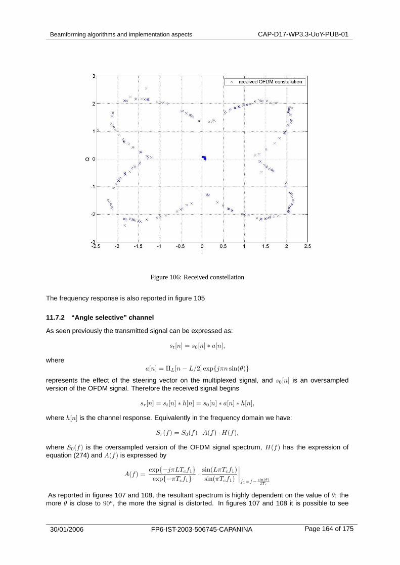
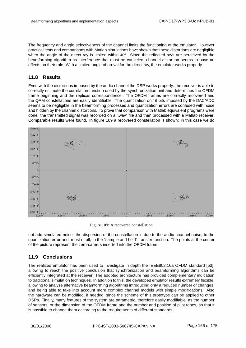
FP6-IST-2003-506745 CAPANINA Deliverable Number D17 Report on adaptive beamforming algorithms for advanced antenna types for aerial platform and ground terminals Document Number CAP-D17-WP3.3-UOY-PUB-01 Contractual Date of Delivery to the CEC 1 st Feb 06 Actual Date of Delivery to the CEC 31 st Jan 06 Author(s): G. White (UOY), E. Falletti (POLITO), Z. Xu (UOY), D. Borio (POLITO), F. Sellone (POLITO), Y. Zakharov (UOY), L. Lo Presti (EUCON), F. Daneshgaran (EUCON) Participant(s) (partner short names): UOY, POLITO, EUCON Editor (Internal reviewer) Marina Mondin Workpackage: WP3.3 Estimated person months 30 Security (PUBlic, CONfidential, REStricted) PUB Nature Report CEC Version 1.1 Total number of pages (including cover): 172 Abstract: This document presents technical descriptions of signal processing and cross-layer algorithm design for beamforming from high altitude platforms (HAPs) to ground terminals, and vice versa, using advanced antenna types - so-called 'smart antennas'. The research covers topics including vertical antenna arrays for communications from HAPs, optimised antenna array beampatterns for cellular coverage from HAPs, array topologies and SINR balancing in adaptive beamforming from HAPs, data communications to trains from HAPs incorporating DOA estimation and tracking methods, LMS-based beamforming with Doppler recovery and RLS- based beamforming for single carrier IEEE 802.16, both focussed towards HAP applications, and the development of a DSP simulator for smart antenna terminals. Keyword list: Smart antennas, HAPs, beamforming, array signal processing, DOA estimation
Transcript
FP6-IST-2003-506745 CAPANINA Deliverable Number D17
Report on adaptive beamforming algorithms for advanced antenna types for aerial platform and ground terminals
Document Number CAP-D17-WP3.3-UOY-PUB-01 Contractual Date of Delivery to the CEC 1st Feb 06
Actual Date of Delivery to the CEC 31st Jan 06
Author(s): G. White (UOY), E. Falletti (POLITO), Z. Xu (UOY), D. Borio (POLITO), F. Sellone (POLITO), Y. Zakharov (UOY), L. Lo Presti (EUCON), F. Daneshgaran (EUCON)
Participant(s) (partner short names): UOY, POLITO, EUCON
Editor (Internal reviewer) Marina Mondin
Workpackage: WP3.3
Estimated person months 30 Security (PUBlic, CONfidential, REStricted)
PUB
Nature Report
CEC Version 1.1
Total number of pages (including cover): 172
Abstract:
This document presents technical descriptions of signal processing and cross-layer algorithm design for beamforming from high altitude platforms (HAPs) to ground terminals, and vice versa, using advanced antenna types - so-called 'smart antennas'. The research covers topics including vertical antenna arrays for communications from HAPs, optimised antenna array beampatterns for cellular coverage from HAPs, array topologies and SINR balancing in adaptive beamforming from HAPs, data communications to trains from HAPs incorporating DOA estimation and tracking methods, LMS-based beamforming with Doppler recovery and RLS-based beamforming for single carrier IEEE 802.16, both focussed towards HAP applications, and the development of a DSP simulator for smart antenna terminals.
Keyword list: Smart antennas, HAPs, beamforming, array signal processing, DOA estimation
antenna types for aerial platform and ground terminals CAP-D17-WP3.3-UOY-PUB-01
31st Jan 06 FP6-IST-2003-506745 CAPANINA Page 2 of 2
DOCUMENT HISTORY
Date Revision Comment Author / Editor Affiliation
31st Jan 06 01 First issue George White UOY
Document Approval (CEC Deliverables only)
Date of
approval Revision Role of approver Approver Affiliation
31st Jan 06 01 Editor (Internal reviewer) Marina Mondin POLITO
31st Jan 06 01 On behalf of Scientific Board
David Grace UOY
Beamforming algorithms and implementation aspects CAP-D17-WP3.3-UoY-PUB-01
30/01/2006 FP6-IST-2003-506745-CAPANINA Page 14 of 175
Beamforming algorithms and implementation aspects CAP-D17-WP3.3-UoY-PUB-01
Executive Summary
The report presents technical descriptions of signal processing and cross-layer algorithm design forbeamforming to and from high altitude platforms (HAPs). The work described was developed for theCapanina project under Workpackage 3.3.
A three-step antenna element weight design process for the optimisation of cellular coverage fora HAP-based antenna array is developed. The technique allows a large set of approximately circularfootprints to be achieved on the ground, even at the edge of the coverage area where the HAP is atan elevation angle of approximately 30o relative to the ground. This footprint circularity improves theability to match footprints to a tesselating hexagonal cellular structure, thus simplifying frequency re-usedesign and improving coverage. It is shown that this technique allows a 424-element antenna array toachieve a coverage performance similar to that of a set of 121 aperture (e.g. horn or lens) antennasreported in [1].
The use of vertical linear (1D) arrays in beamforming from HAPs is investigated. A HAP-mountedvertical antenna allows the generation of a set of concentric ring-shaped cells over a coverage area.Coverage performance is compared again with the set of 121 aperture antennas reported in [1]. It isshown that a vertical antenna can achieve an improvement in coverage performance by up to 20 dBand can even support more cells for one channel with the same number of antenna elements comparedwith the set of aperture antennas.
Array topologies for adaptive (Capon) beamforming from HAPs are investigated in conjunction withthe effects of non-Gaussian element phase errors that may be experienced in a HAP scenario, for exam-ple due to HAP attitudinal variations. It is shown that circular antenna arrays may have distinct advan-tages when used to implement Capon beamforming from HAPs. A circular array with half-wavelengthelement spacing, when Capon beamforming is applied, suffers less variation in antenna gain as afunction of angular separation of interferers than square arrays with either half-wavelength spacing orequivalent half-power beamwidth (HPBW). Additionally, circular arrays may aid array calibration throughthe use of radial RF element feeds.
A channel allocation method is developed which can be applied to the space-time scheduling prob-lem in a HAP scenario. The large number of simultaneous users in a HAP coverage area (100’s or1000’s) prohibits both the use of exhaustive searches for optimal channel allocations and suboptimalstrategies proposed thus far in the literature for terrestrial base-stations. The method proposed isbased purely on the spatial distribution of the users in the coverage area, is fast, deterministic andyields capacity improvements of up to 75% relative to random channel assignments, in the presence ofnon-Gaussian element phase errors (e.g. HAP attitudinal variation).
The use of SINR balancing in the HAP communications scenario is investigated. An iterativeeigendecomposition-based algorithm which jointly estimates transmit power levels and weight vectorsso as to balance SINR for a set of users is applied to the HAP downlink. It is shown that SINR balancingcan be beneficial in the scenario, reducing the probability of very low SINR for some users. However,this is only the case when used in conjunction with a channel allocation algorithm, such as that pro-posed in the report, which can reduce the probability of closely-spaced users being allocated the sametime- or frequency-channel.
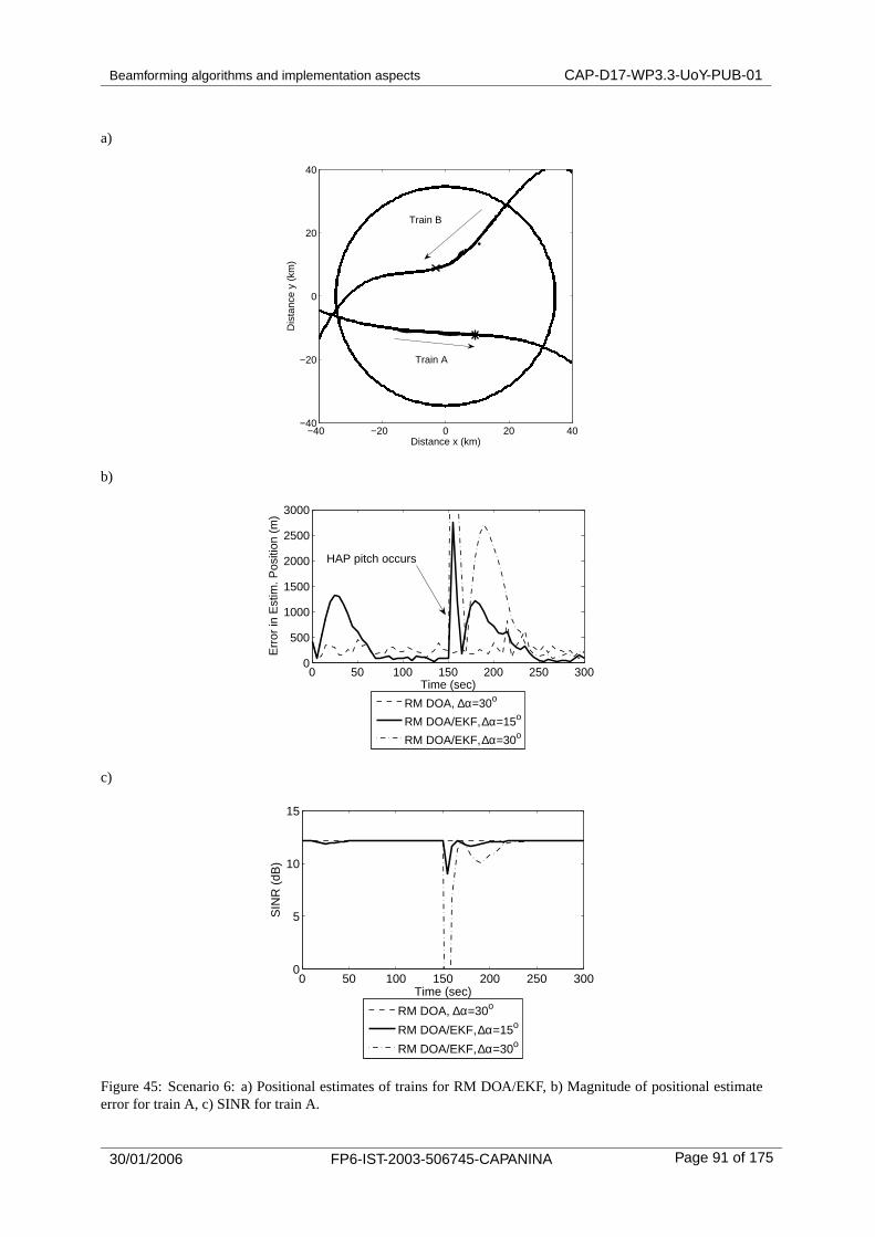
The viability of providing high-data rate communications to train users from HAPs, as an alternativeto satellite links, is demonstrated. Methods for estimation of the number of sources, DOA estimation,DOA tracking and reliable attribution of data estimates to trains are explored in a range of train scenariosusing a HAP-based smart antenna. It was shown that extended Kalman filtering (EKF) ensures reliableattribution of DOA estimates to trains, particularly when trains pass closely or cross. EKF can beparameterised so as to follow slow variations in train velocity whilst simultaneously being stable tosudden HAP motion. Null-steering is shown to be beneficial in HAP-train data communications even forsmall numbers of trains.
A classical Least Mean Square (LMS) beamforming algorithm is developed for application to OFDMtransmission, and in the process a new approach which is Doppler resilient is derived. In order toensure low computational complexity, a pre-FFT modified LMS beamforming algorithm is adopted. Inorder to totally cancel out the Doppler effect, an estimate of the Doppler frequency is included into thecost function. Besides, in order to cope with the noise impairment at low signal-to-noise ratios, thepart of the cost function due to the zero-subcarriers is replaced with a similar term which considers
30/01/2006 FP6-IST-2003-506745-CAPANINA Page 15 of 175
Beamforming algorithms and implementation aspects CAP-D17-WP3.3-UoY-PUB-01
an estimation of the noise power. This last version of the algorithm is Doppler resilient and avoidscompression of the constellation.
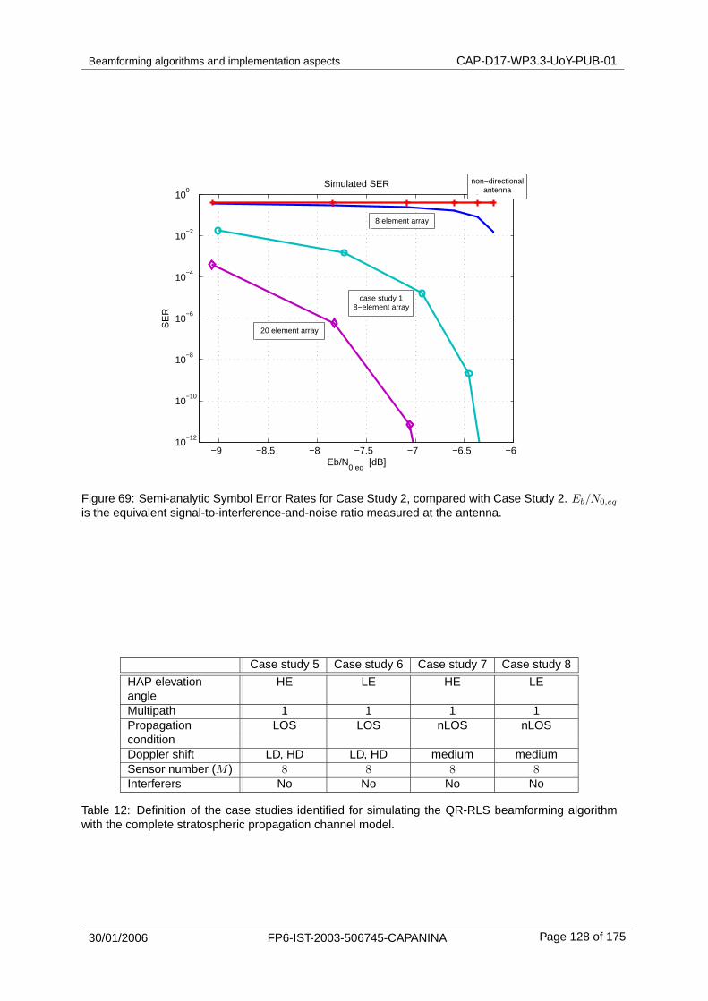
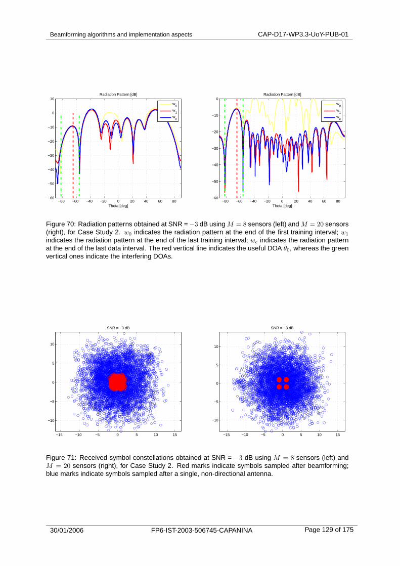
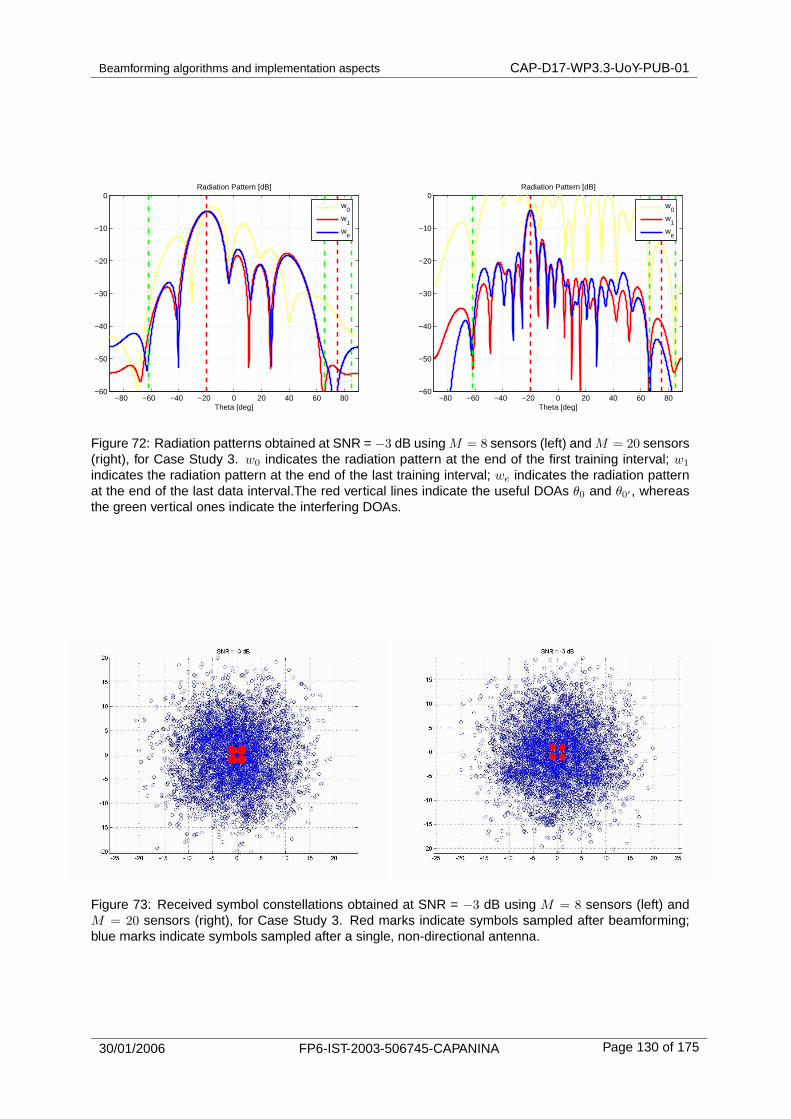
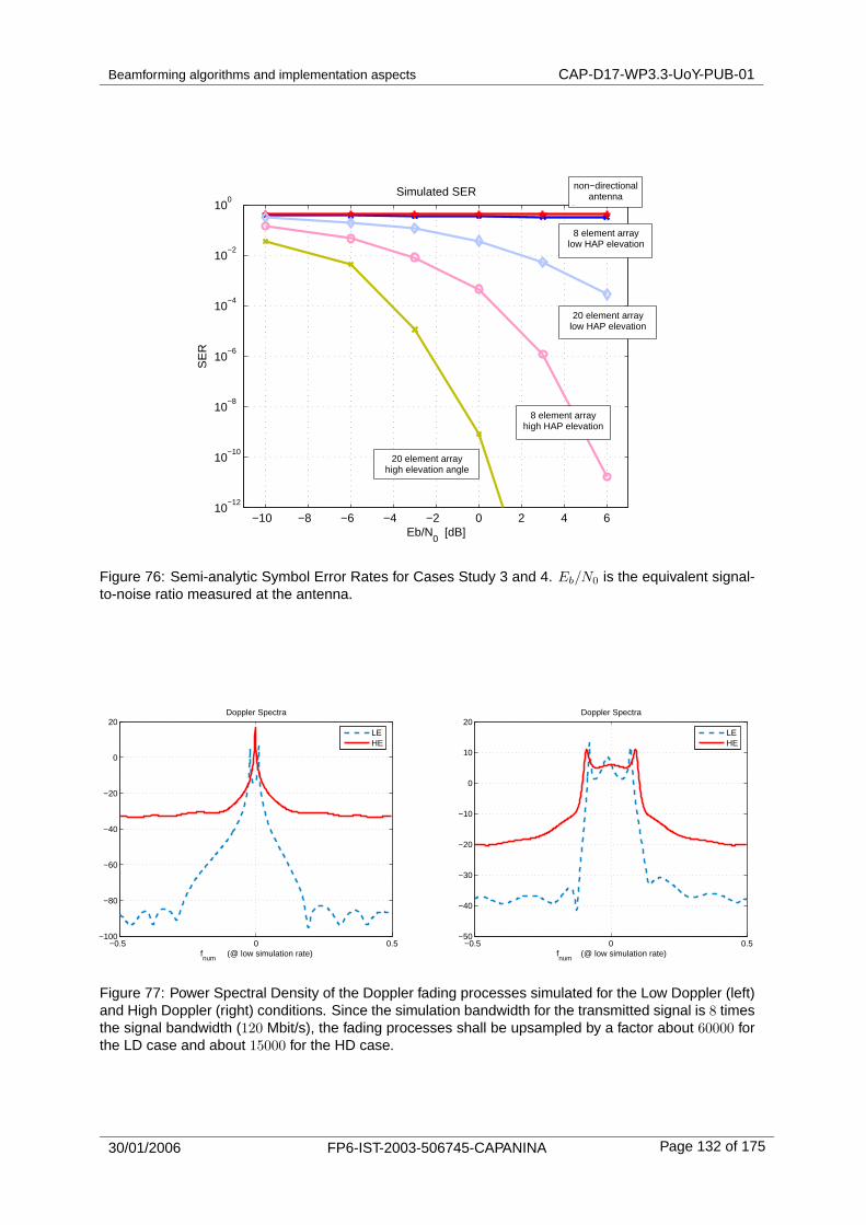
A numerically robust Doppler-resilient beamforming algorithm is developed for ground terminal ar-ray antennas, either stationary or mobile. The approach is based on an RLS solution, which alternatesbetween a trained and a decision-directed mode. Furthermore, the numerical robustness of the algo-rithm is guaranteed by its QR implementation. Infinite precision performance is tested in this report bysimulation, for different propagation impairments including multipath, Doppler shift, fast fading, and in-terference. In particular, very promising results are obtained when the beamforming algorithm is appliedover the complete CAPANINA short-term propagation channel model [2].
A novel antenna array calibration algorithm is presented. The algorithm counteracts performanceimpairment due to sensor coupling in both DOA estimation and beamforming algorithms. The proposedalgorithm does not require knowledge of the signals emitted by the sources, nor their direction of arrival(DOA) but, instead, can be embedded within any classical super-resolution DOA estimation algorithmto simultaneously estimate the coupling parameters as well as the DOAs. Computer simulations showthe effectiveness of the proposed technique, which is able to restore the desirable statistical propertiesof DOA estimation algorithms such as MUSIC, even in the presence of coupling.
A smart antenna DSP emulator to investigate beamforming within the IEEE802.16a OFDM standardis developed. The adopted architecture provides research results that are complementary to traditionalsimulation techniques. In addition to this, the emulator is extremely flexible, allowing analysis of alter-native beamforming algorithms with a minimum number of changes; the emulator can be modified formore complex channel models, again with only simple modifications. Also the hardware can be mod-ified, if needed, since the system is not specific to an individual DSP platform. Finally, many featuresof the system are parametric and therefore easily modifiable: such as the number of sensors, or thedimension of the OFDM frame and the number and position of pilot tones. It is possible to changethese parameters according to the requirements of different standards. It is shown that it is not possibleto achieve a 120 Mbit/s bit-rate with a DSP working at 100 MHz clock, due to limitations in frequencysampling of the audio DAC and ADC of the DSP boards.
30/01/2006 FP6-IST-2003-506745-CAPANINA Page 16 of 175
Beamforming algorithms and implementation aspects CAP-D17-WP3.3-UoY-PUB-01
1 Introduction
1.1 Overview of report
This report presents a set of novel investigations into advanced beamforming algorithms for HAP-based communications. Figure 1 provides a diagrammatic overview of the report. The investigationsinclude algorithms for both HAP-based smart antennas (Chapters 2-7) and ground-based smart an-tennas (Chapters 8-11). The investigations also cover the two key Capanina applications: broadbandaccess for rural areas (Chapters 2-6) and for trains (Chapter 7). The two applications are investigatedjointly in the algorithms in Chapters 8-11. Similarly, the research work presented here covers both datalink and physical layers, with investigations of channel allocation (Chapter 5), power control (Chapters 4and 7), algorithms for signal processing (all chapters), DSP implementation (Chapter 11), beampatternoptimisation (Chapters 2-4 and 7-9) and link budget (Chapters 4 and 7). An additional categorisation isbetween non-adaptive methods, which are of relatively low complexity (Chapters 2 and 3), and adap-tive methods of higher complexity (all other Chapters). A key issue relating to practical performance ofsmart antennas, that of array calibration, is addressed in Chapter 10.
Figure 1: Outline of Deliverable 17
1.2 Background to HAP-related beamforming
High altitude platforms, HAPs, are aeroplanes or airships proposed for stationing at stratospheric al-titudes (17-22km) in order to provide communications or monitoring services [3] [4]. HAPs offer thepotential of smaller cell areas - and therefore higher capacity - than satellite systems, along with lowerfree-space path loss and shorter propagation delays. HAPs could also alleviate the need for largenumbers of terrestrial base stations and facilitate rapid roll-out of broadband services in areas with littleexisting communications infrastructure.
Beamforming is a process whereby advanced antenna arrays, so-called smart antennas, are used inconjunction with signal processing techniques to provide a beampattern which is in some way optimised(e.g. [5]). Smart antennas have been proposed in existing research for the steering of beampatternpeaks towards a desired source - ’beam-steering’, for steering nulls towards sources of interference -’null-steering’, and for the determination of the directions of arrival (DOAs) of sources - ’DOA estimation’.
30/01/2006 FP6-IST-2003-506745-CAPANINA Page 17 of 175
Beamforming algorithms and implementation aspects CAP-D17-WP3.3-UoY-PUB-01
Existing work on beamforming for terrestrial base-stations has typically concerned itself only withazimuthal beamforming (from 0o to 360o) using 1D (linear) arrays. For example, 1D mobility trackingin terrestrial cellular networks using base-stations equipped with smart antennas has been researchedrecently in several sources, e.g. [6] [7] [8]. Achieving high antenna gain to satisfy the link budget is nottypically the major concern in terrestrial cellular scenarios; thus only small arrays have been consideredin much existing research. As a result, many of the smart antenna signal processing and cross-layeralgorithm designs in existing literature are too complex to be implemented in a HAP scenario, in which alarger number of antenna elements are needed for higher gain and there are large numbers of users inthe coverage area. As an example, channel allocation methods for smart antennas described in [9], [10]and [11] are implementable only in a terrestrial base station scenario in which the total number of usersin the system, and the number of users per channel, can be assumed to be relatively small.
Satellite adaptive beamforming [12] [13] requires beamforming in azimuth and elevation using 2D(planar) arrays. For smart antennas mounted on geostationary earth orbiting (GEO) satellites, scanningwould be restricted to small angular ranges; from 0o to 360o in azimuth but only over a few degrees in ele-vation from the normal to the array, due to the large distance of the Earth from the satellite (≈36000km).Overcoming free-space path loss for GEO satellite links, however, is a major concern due to the longlink length - antenna arrays with very large numbers of elements are needed to achieve sufficient an-tenna gain to mitigate path loss. The large numbers of antenna elements could in theory facilitatenull-steering to large numbers of users in a satellite coverage area, although computational complexityfor such a large number of elements may make the approach difficult to apply in practice [13].
Beamforming for HAP-based communications is, in comparison to terrestrial- and satellite-basedbeamforming, a relatively unexplored field. In [14], a 4 × 4 element antenna array for adaptive beam-forming was developed for HAP-based DOA estimation in the 31/28GHz band. A signal processingalgorithm for controlling weighting of a set of fixed beams was developed as a low complexity imple-mentable method. A localisation system for mobile phone users from HAPs was described in [15] usinga HAP-based smart antenna employing polynomial-based beamspace direction-of-arrival (DOA) esti-mation. The paper focussed on satisfying emergency localisation criteria for a single stationary mobileuser rather than beamforming for high data-rate communications to trains and rural areas, which is thefocus under Capanina.
Provision of high data rate communications services to train travellers has been a topic of muchrecent research interest, e.g. [16] [17], resulting in the emergence of internet access based on wirelesslocal area networks (WLANs) on some commercial train routes, e.g. [18] [19]. Existing services aretypically realised using a combination of geostationary satellite and terrestrial cellular links; satellitelinks being used to provide higher speed connections where line-of-sight to geostationary earth orbiting(GEO) satellites is available, whilst multiple terrestrial cellular links are often exploited to maintain lowerspeed connections when trains are in stations or tunnels. Data rate and capacity of existing services islimited by the performance of the satellite link, which is reliant in the case of [19] on a single large an-tenna footprint covering most of Western Europe [20]. The use of HAPs equipped with smart antennascould help to solve these capacity problems by providing steerable coverage (and tracking) to multipletrains simultaneously; this is explored in Chapter 7.
Beamforming from HAPs requires scanning in both azimuth and elevation over large angular ranges;the analyses in this report use scanning/beamforming for azimuthal angles from 0o to 360o and elevationangles from 0o (to sub platform point) to 60o (to edge of coverage). This makes planar arrays a naturalchoice, although the investigation in Chapter 3 shows how coverage from a HAP can be achieved witha low complexity vertical linear array. Due to the shorter link length for HAPs (20-40 km) compared toGEO satellites, antenna arrays with smaller numbers of elements can be used at the HAP to satisfy thelink budget. Thus, relative to satellites, more advanced beamforming algorithms can be explored.
Investigations of robust beamforming from HAPs and beamforming to multiple HAPs from smallportable ground terminal smart antennas will be incorporated into the final deliverable in this workpack-age: D28, ”Report detailing the implementation aspects of signal processing for aerial platform andground terminal beamformers”.
30/01/2006 FP6-IST-2003-506745-CAPANINA Page 18 of 175
Beamforming algorithms and implementation aspects CAP-D17-WP3.3-UoY-PUB-01
1.3 Complexity considerations
In the report overview above, the categorisation was made between non-adaptive methods, which areof relatively low complexity (Chapters 2 and 3), and adaptive methods of higher complexity (all otherChapters).
Chapter 2 proposes a non-adaptive antenna array with 424 elements, to demonstrate performancewhich is better than a set of 121 aperture (e.g. lens or horn) antennas [21]. The method proposed hereapplies pre-determined, static weightings of amplitude and phase to signals at the antenna elements,and so, in theory, can be applied without converting all element signals to baseband. It is the authors’belief that the 424-element 31/28GHz non-adaptive array of omni-directional elements (e.g. a patchantenna array) proposed here should still prove less bulky as a HAP payload than the set of 121 distinctaperture antennas proposed in [21]. However, design and development of such large patch antennaarrays is an area for future research.
Chapters 4 - 7 focus on 64 element (8 × 8) smart antenna arrays. Effective adaptive techniquestypically require processing complexity O(M3) per beam per estimation process, where M is the num-ber of antenna elements. Reduced complexity methods for solution of linear systems of equations [22]have been recently proposed, which should make adaptive methods for larger smart antenna arraysmore realisable in terms of baseband processing complexity. In addition to the baseband processingcomplexity, smart antennas for adaptive beamforming require radio-frequency (RF) front-end circuitryfor each element of the array; this can cause smart antenna hardware to become restricted in space forcircuitry, particularly at frequencies above 20GHz, e.g. [12]. It is noted that 4 × 4 smart antennas havebeen successfully constructed in [12] and [14], and that an 8× 8 array is being constructed as part of afollow-on project to [12]. Array calibration was noted as a problem in [14], although a method for copingwith the problem has been proposed here in Chapter 10.
1.4 Dissemination of results
The following papers relating to research in this document have been either submitted or accepted:
Z. Xu, G. White, and Y. Zakharov, ”Optimization of beampattern of High Altitude Platform antennausing conventional beamforming,” accepted by IEE Proc. Communications, February 2005.
Z. Xu and G. White, ”Optimizing the beam pattern of High Altitude Platform antenna arrays,” in Proc.of Postgraduate Symposium on the Convergence of Telecommunications, Networking and Broadcast-ing (PGNET 2005), Liverpool, UK, pp. 101-106, June 2005.
Z. Xu, Y. Zakharov, and G. White, ”Vertical antenna array and spectral reuse for ring-shaped cellularcoverage from High Altitude Platform,” accepted by Loughbourgh Antennas and Propagation Confer-ence (LAPC 2006), November 2005.
Z. Xu, Y. Zakharov, and G. White, ”Vertical linear antenna arrays for ring-shaped cellular coveragefrom High Altitude Platforms,” submitted to IEEE Communications Letters, November 2005.
G. White, Y. Zakharov and J. Thornton, ”Array topologies for High Altitude Platform smart antennas”,in Proc. of Wireless Personal and Multimedia Communications (WPMC 2005), Aalborg, Denmark, Sept17th-22nd, 2005.
G. White and Y. Zakharov, ”Data communications to trains from High Altitude Platforms”, submittedto IEEE Trans. on Vehicular Technology, September 2005.
F. Sellone and A. Serra, ”A novel on-line calibration method for uniform and linear arrays,” submittedto IEEE Trans. on Signal Processing, August 2005.
30/01/2006 FP6-IST-2003-506745-CAPANINA Page 19 of 175
Beamforming algorithms and implementation aspects CAP-D17-WP3.3-UoY-PUB-01
E. Falletti, L. Rega, F. Sellone, M. Urso, ”A Doppler-resilient QRD-RLS beamforming algorithm forOFDM communications with High altitude platforms”, submitted to IST Summit on Mobile and WirelessCommunications 2006, Mykonos, Greece, June 2006.
30/01/2006 FP6-IST-2003-506745-CAPANINA Page 20 of 175
Beamforming algorithms and implementation aspects CAP-D17-WP3.3-UoY-PUB-01
2 Optimised antenna array beampatterns for HAP coverage
2.1 Background to conventional beamforming methods
Conventional beamforming can be divided into several approaches based on the type of antennas thatare used. One approach, fixed multi-beam, involves generating a set of beams by using a set of distinctaperture antennas, such as horn, lens or reflector antennas, to provide one spot beam per cell [21].Cell size is determined by beampattern of the individual antennas. Aperture antennas can achievebeampatterns with low sidelobes levels and improve the system capacity [21]. But the antenna sizeand weight could be significant, which means that a large, heavy system payload may be required. Thismay be a problem for many HAPs. Furthermore, mechanical steering of the antennas, to compensatefor HAP motion, could be a problem.
In this chapter, we will focus on HAP beamforming based on an antenna array. The research con-cerns applying weights to the array elements to steer a set of beams in order to form cells on the ground.This is similar to the use of a set of distinct aperture antennas as in [21], but the key advantages wouldbe reduced size and weight and more flexibility for system configuration.
Much research has been conducted recently in the area of conventional beamforming using antennaarrays. A method is developed in [23] to optimize element weights to suppress sidelobes to below -30dB, whilst maintaining a narrow mainlobe. This technique relies on non-uniform element spacing spe-cific to a desired steering direction and therefore is difficult for optimizing multiple beams simultaneously.In [24], sub-array techniques are applied for a beam-steerable antenna. It is shown that using sub-arraytechniques can drastically reduce the fabrication complexity of phased array systems. The array sizeand manufacturing costs can also be reduced. However, sidelobe levels, controlled at -20 dB, may notbe sufficiently suppressed for many applications. In [25], a method is proposed based on defining aspatial masking filter according to a desired beampattern, calculating the antenna aperture distributionwhich corresponds to both the masking filter and the aperture size, and finally spatially sampling theaperture distribution at the antenna element positions. The advantage is that a beampattern with arbi-trary geometry can be generated, which is useful in Capanina project where we may wish to maximisecoverage by creating a set of closely-tesselating cellular footprints on the ground. The weakness of themethod as described in [25] is that the results are very sensitive to the choice of the masking filter.Furthermore, in a HAP scenario, when power is steered to a position far away from the center of thecoverage area, the results using the method in [25] are poor and the shape of the footprint is far fromthe desire one. In this chapter we describe modifications to the method which allow coverage optimisa-tion to be achieved in a HAP scenario, such that the method may prove more beneficial for HAP-basedbeamforming than the use of a set of aperture antennas in [21].
2.2 Project motivation
In this chapter, we apply the method from [25] for optimizing antenna array weights in order to obtainarbitrary cell shapes (as defined by beam footprints on the ground) and to obtain low sidelobe levels.Specifically, we are interested in the provision of equal-size circular footprints on the ground. Themotivation for this is the development of a tessellating structure of cells that maximises the coverage,while simplifying bandwidth reuse planning [1]. The following refinements to the method in [25] areintroduced: 1) first, a ground masking filter corresponding to the desired cell shape, is defined andthen it is transformed to an angle masking filter; 2) a two-dimensional Gaussian function is used asthe ground masking filter to reduce the effect of sharp boundaries; 3) the parameters of the maskingfilter are adjusted to achieve footprints close to circular while obtaining a good compromise betweenmainlobe width and sidelobe levels. We show that this approach allows a 424-element antenna array toachieve a coverage performance similar to that previously reported for 121 lens aperture antennas [1],with an expected reduction in mass payload.
2.3 Communications scenario
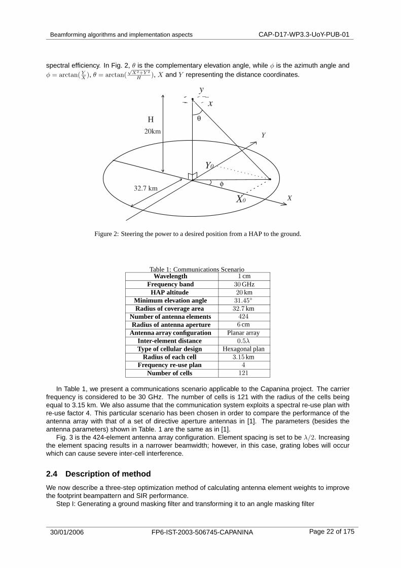
Fig. 2 illustrates a communication scenario with a HAP at an altitude of H = 20 km providing coverageover a circular area with radius of 32.7 km. This coverage area is divided into cells in order to maximise
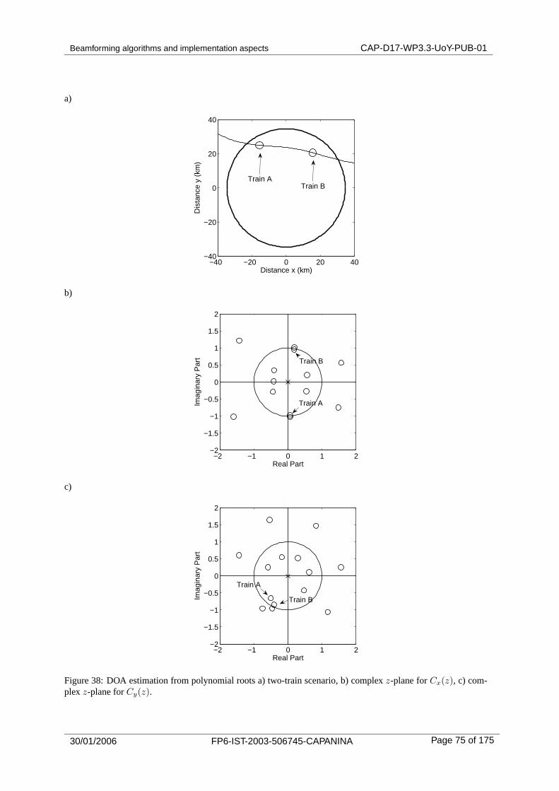
30/01/2006 FP6-IST-2003-506745-CAPANINA Page 21 of 175
Beamforming algorithms and implementation aspects CAP-D17-WP3.3-UoY-PUB-01
spectral efficiency. In Fig. 2, θ is the complementary elevation angle, while φ is the azimuth angle andφ = arctan( Y
X ), θ = arctan(√
X2+Y 2
H ), X and Y representing the distance coordinates.
φ
θ
X
Y
32.7 km
20km
H
y
x
Y0
X0
Figure 2: Steering the power to a desired position from a HAP to the ground.
Table 1: Communications ScenarioWavelength 1 cm
Frequency band 30 GHzHAP altitude 20 km
Minimum elevation angle 31.45
Radius of coverage area 32.7 kmNumber of antenna elements 424Radius of antenna aperture 6 cm
Antenna array configuration Planar arrayInter-element distance 0.5λType of cellular design Hexagonal plan
Radius of each cell 3.15 kmFrequency re-use plan 4
Number of cells 121
In Table 1, we present a communications scenario applicable to the Capanina project. The carrierfrequency is considered to be 30 GHz. The number of cells is 121 with the radius of the cells beingequal to 3.15 km. We also assume that the communication system exploits a spectral re-use plan withre-use factor 4. This particular scenario has been chosen in order to compare the performance of theantenna array with that of a set of directive aperture antennas in [1]. The parameters (besides theantenna parameters) shown in Table. 1 are the same as in [1].
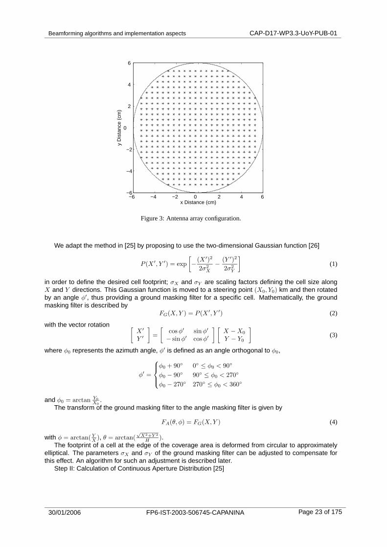
Fig. 3 is the 424-element antenna array configuration. Element spacing is set to be λ/2. Increasingthe element spacing results in a narrower beamwidth; however, in this case, grating lobes will occurwhich can cause severe inter-cell interference.
2.4 Description of method
We now describe a three-step optimization method of calculating antenna element weights to improvethe footprint beampattern and SIR performance.
Step I: Generating a ground masking filter and transforming it to an angle masking filter
30/01/2006 FP6-IST-2003-506745-CAPANINA Page 22 of 175
Beamforming algorithms and implementation aspects CAP-D17-WP3.3-UoY-PUB-01
−6 −4 −2 0 2 4 6 −6
−4
−2
0
2
4
6
x Distance (cm)
y D
ista
nce
(cm
)
Figure 3: Antenna array configuration.
We adapt the method in [25] by proposing to use the two-dimensional Gaussian function [26]
P (X ′, Y ′) = exp
[− (X ′)2
2σ2X
− (Y ′)2
2σ2Y
](1)
in order to define the desired cell footprint; σX and σY are scaling factors defining the cell size alongX and Y directions. This Gaussian function is moved to a steering point (X0, Y0) km and then rotatedby an angle φ′, thus providing a ground masking filter for a specific cell. Mathematically, the groundmasking filter is described by
FG(X,Y ) = P (X ′, Y ′) (2)
with the vector rotation [X ′
Y ′
]=
[cos φ′ sinφ′
− sin φ′ cos φ′
] [X − X0
Y − Y0
](3)
where φ0 represents the azimuth angle, φ′ is defined as an angle orthogonal to φ0,
φ′ =
φ0 + 90 0 ≤ φ0 < 90
φ0 − 90 90 ≤ φ0 < 270
φ0 − 270 270 ≤ φ0 < 360
and φ0 = arctan Y0
X0.
The transform of the ground masking filter to the angle masking filter is given by
FA(θ, φ) = FG(X,Y ) (4)
with φ = arctan( YX ), θ = arctan(
√X2+Y 2
H ).The footprint of a cell at the edge of the coverage area is deformed from circular to approximately
elliptical. The parameters σX and σY of the ground masking filter can be adjusted to compensate forthis effect. An algorithm for such an adjustment is described later.
Step II: Calculation of Continuous Aperture Distribution [25]
30/01/2006 FP6-IST-2003-506745-CAPANINA Page 23 of 175
Beamforming algorithms and implementation aspects CAP-D17-WP3.3-UoY-PUB-01
The aperture distribution K(ρ, φ) can be expressed by the Fourier series:
K(ρ, β) =
∞∑
n=−∞Kn(ρ)ejnβ (0 ≤ ρ ≤ r , 0 ≤ β ≤ 2π) (5)
where ρ and β are the radial and angular coordinates of a circular aperture with radius r. The Fouriercoefficients Kn(ρ) can be derived as:
Kn(ρ) =π
2r2(j)n
∫ 2r/λ
0
φn(ω)Jn(ωρ)ωdω (6)
where ω = 2rλ sin θ, Jn(·) is the nth order Bessel function of the first kind and φn(ω) is the Fourier
transform of the Gaussian masking filter designed in Step I,
φn(ω) =1
2π
∫ π
−π
FA(θ, φ)ejnφdφ (7)
where, φ is the azimuth angle, and FA(θ, φ) is given by (4). Since we cannot calculate an infinite numberof Fourier terms in (5), the series should be truncated to obtain an approximation K(ρ, β). Then (5) canbe rewritten as a finite Fourier series
K(ρ, β) =
+M∑
n=−M
Kn(ρ)ejnβ . (8)
In general, an increase in M leads to better approximation accuracy but it also significantly increasesthe computation time. In our simulation below, where the number of elements of the antenna array is424, M is set to be 500; this is enough for our scenario to provide sufficient approximation accuracy.
Step III: Sampling the aperture distribution onto a pre-designed planar arrayEach antenna element is assigned a complex weight by spatial sampling:
w(n) = K(ρn, βn), n = 1, . . . , N, (9)
where the position of each antenna element is defined within an aperture of radius r.Efficient spectral re-use in wireless telecommunications systems is often achieved by using a cellular
coverage strategy. Fig. 4 is an example of 121 cells with frequency re-use factor 4. Cells that share thesame spectral channel are marked by the same number and are termed co-channel cells; each cell hasa different spectral channel to its neighbours. The shaded cells are those that share channel 3. Theseare selected to investigate the performance of the antenna array using the proposed method. The redcircle represents the maximum limit of the footprint size. If the footprint exceeds this limit, co-channelinterference will significantly reduce system capacity.
We now propose a method for choosing the parameters of the 2D Gaussian function (1), thusdefining the ground masking filter for a specific cell. Firstly, the maximum of the Gaussian function ispositioned in the center of the cell; this defines the parameters X0 and Y0 in (3). Secondly, we aimto find optimum values for σX and σY , controlling the beamwidth and sidelobe levels, to reduce co-channel interference. The relationship between σX and σY affects the shape of the cell footprint. Thisrelationship depends only on the distance between the cell center and the center of the HAP coveragearea. In the center point of the coverage area, σX and σY should be equal to achieve a circular cellshape. Computational experiments have shown that for a 424-element antenna array arranged as acircular planar array, σY should be 1.2 times larger than σX at the boundary of the coverage area. Atother positions, this relationship can be approximated by a linear function of the distance. Thus, theshape of the cell footprints can be approximately controlled to be circular for all cells. Taking this intoaccount, the only parameter to be found is σX . Let σ0 be an initial value of σX , and ε be an accuracymetric for determining the optimal value of σX . The algorithm for optimizing σX is described by thefollowing steps:
1. Initialize σX = σ0 and a parameter ∆=σ0/2.
30/01/2006 FP6-IST-2003-506745-CAPANINA Page 24 of 175
Beamforming algorithms and implementation aspects CAP-D17-WP3.3-UoY-PUB-01
−35 −25 −15 −5 5 15 25 35
−30
−20
−10
0
10
20
30
3 2 3 2 3 2 3 2 3 2 3
1 4 1 4 1 4 1 4 1 4 1 4
2 3 2 3 2 3 2 3 2 3 2
1 4 1 4 1 4 1 4 1 4
2 3 2 3 2 3 2 3 2
1 4 1 4 1 4 1 4
3 2 3 2 3
4 1 4 1 4 1 4 1 4 1 4 1
2 3 2 3 2 3 2 3 2 3 2
4 1 4 1 4 1 4 1 4 12 3 2 3 2 3 2 3 2
4 1 4 1 4 1 4 1
3 2 3 2 3
X Distance (km)
Y D
ista
nce
(km
)
Figure 4: 121 hexagonal cells configuration.
2. If ∆ ≤ ε, choose σx and end this process. Otherwise, calculate σx +∆ and σx −∆ and determinethe average power at all co-channel cells except the steering cell.
3. Compare the average powers for σx +∆, σx and σx−∆ and find a minimum Pmin among them. Ifσx provides the minimum power, go to step 5; if σx+∆ or σx−∆ provides the minimum, go, respectively,to step 4a or step 4b.
4a. Increase σx, σx +n∆ (n = 1, 2, · · · ), calculate the average power in co-channel cells and updatethe minimum Pmin until the average power becomes larger than the current minimum value.
4b. Decrease σx, σx−n∆ (n = 1, 2, · · · ), calculate the average power in co-channel cells and updatethe minimum Pmin until the average power becomes larger than the current minimum value.
5. Reduce ∆, ∆ = ∆/2, and go to step 2.This algorithm finds the optimum parameters for the masking filter to achieve minimum average
sidelobe levels in ground co-channel cells.
2.5 Simulation results
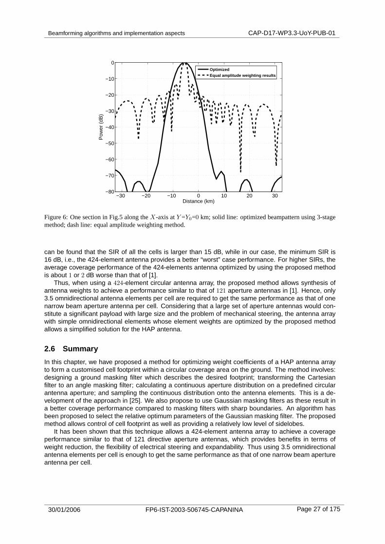
First, we use the antenna array shown in Fig. 3 and steer the power to the cell with the center atX0 = −5.46 km and Y0 = 0 km. The footprint of the beampattern is shown in Fig. 5. Fig.6 comparesa section of the footprint along the X axis at Y = Y0 with that of the array when uniform amplitudeweightings are applied to elements. The proposed method allows a significantly lower sidelobe level (-67 dB) with respect to the case of uniform amplitude weighting. However, it is noted that the beamwidthis increased relative to the uniform amplitude weighting case, the effects of which can be mitigatedthrough appropriate choice of spectral re-use factor.
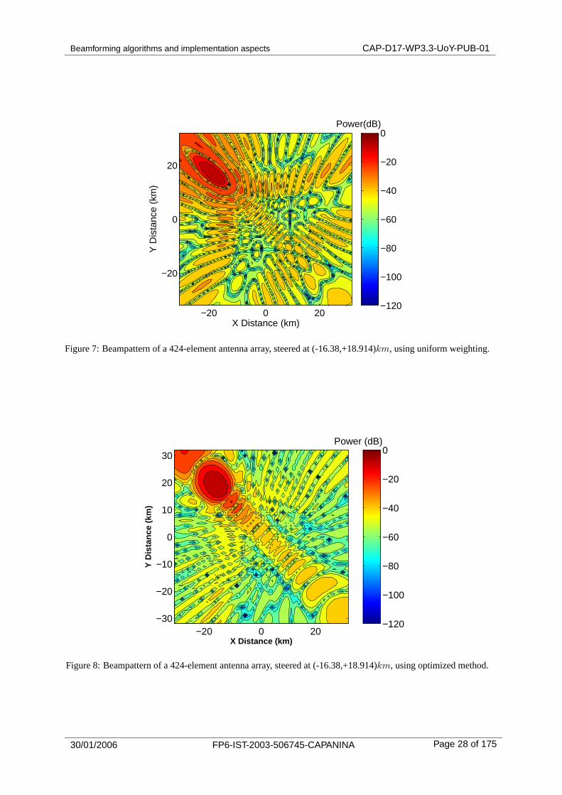
Next we consider a situation where the cell is further away from the center of the coverage area; wechoose a cell center at X0 = −16.38 km and Y0 = +18.914 km. Fig. 7 is the result of uniform amplitudeweighting and it is used to compare with our optimized result, shown in Fig. 8 and Fig. 9. Sidelobesare suppressed to approximately −39 dB. Although the overall performance is worse than the previousexample, where the cell was close to the center of the coverage area, the proposed method provides asignificantly better sidelobe suppression than the uniform magnitude weighting. The footprint shape inFig. 8 is also closer to circular when compared with the uniform amplitude weighting in Fig. 7.
Fig. 10 shows footprints of all channel-3 cells. It is seen that the footprints are approximately circularat any cell location within the coverage area.
30/01/2006 FP6-IST-2003-506745-CAPANINA Page 25 of 175
Beamforming algorithms and implementation aspects CAP-D17-WP3.3-UoY-PUB-01
Power (dB)
X Distance (km)
Y D
ista
nce
(km
)
−20 0 20−30
−20
−10
0
10
20
30
−120
−100
−80
−60
−40
−20
0
Figure 5: optimized beampattern of a 424-element antenna array, steered at (-5.46,+0)km.
We now investigate the communications performance by analyzing the relationship between cov-erage and SIR. First, cells are divided amongst several channels using a frequency re-use plan. As-sume that there are Nc cells that share the same channel and users are randomly positioned in theseco-channel cells. Then a HAP antenna steers Nc beams to these co-channel cells. The user of inter-est at the ground position θ (defined by the complementary elevation angle) receives powers Pri(θ),i = 1, . . . , Nc, from these beams. Considering the link budget for the HAP-Earth link, the power (in dB)received from one beam can be represented as [27]
Pr(θ) = Pt + Gd(θ) − Lt − Lr − Ls(θ) (10)
Gd(θ) =4πF (θ)
∫ +π/2
−π/2F (θ) cos θdθ
(11)
and
Ls(θ) = 20log10(4πH
λ cos θ) (12)
where Gd(θ) and Ls(θ) represent the transmit antenna directivity and free-space path loss, respectively.Pt is the transmit power, Lt the transmit antenna loss and Lr represents the rain margin. Within thesereceived Nc beams, one forms the cell with the user of interest, the power of which is denoted byPrmax(θ). For the user of interest, the SIR can be defined by [1]:
SIR(θ) =Prmax(θ)
−Prmax(θ) +∑Nc
i=1 Pri(θ). (13)
In this case, one user has one value of SIR and average coverage performance can be quantified as thefractional area of all the users SIR values in the co-channel cell groups served at a given SIR threshold.
Fig. 11 shows the coverage performance of the 424-element antenna array shown in Fig. 3 andcompares the performance with results achieved by a set of distinct aperture antennas in [1]. In Fig. 11,the solid line from [1], corresponds to the coverage performance provided by 121 lens aperture antennasunder the assumption that the sidelobes are modeled as a flat floor at -40 dB for all antennas includingthose directed to the cell at the edge of the coverage area. Other curves represent the best, worst andaverage coverage performance achieved by the 424-element antenna array. From the results in [1], it
30/01/2006 FP6-IST-2003-506745-CAPANINA Page 26 of 175
Beamforming algorithms and implementation aspects CAP-D17-WP3.3-UoY-PUB-01
−30 −20 −10 0 10 20 30−80
−70
−60
−50
−40
−30
−20
−10
0
Distance (km)
Pow
er (
dB)
OptimizedEqual amplitude weighting results
Figure 6: One section in Fig.5 along theX-axis atY =Y0=0 km; solid line: optimized beampattern using 3-stagemethod; dash line: equal amplitude weighting method.
can be found that the SIR of all the cells is larger than 15 dB, while in our case, the minimum SIR is16 dB, i.e., the 424-element antenna provides a better “worst” case performance. For higher SIRs, theaverage coverage performance of the 424-elements antenna optimized by using the proposed methodis about 1 or 2 dB worse than that of [1].
Thus, when using a 424-element circular antenna array, the proposed method allows synthesis ofantenna weights to achieve a performance similar to that of 121 aperture antennas in [1]. Hence, only3.5 omnidirectional antenna elements per cell are required to get the same performance as that of onenarrow beam aperture antenna per cell. Considering that a large set of aperture antennas would con-stitute a significant payload with large size and the problem of mechanical steering, the antenna arraywith simple omnidirectional elements whose element weights are optimized by the proposed methodallows a simplified solution for the HAP antenna.
2.6 Summary
In this chapter, we have proposed a method for optimizing weight coefficients of a HAP antenna arrayto form a customised cell footprint within a circular coverage area on the ground. The method involves:designing a ground masking filter which describes the desired footprint; transforming the Cartesianfilter to an angle masking filter; calculating a continuous aperture distribution on a predefined circularantenna aperture; and sampling the continuous distribution onto the antenna elements. This is a de-velopment of the approach in [25]. We also propose to use Gaussian masking filters as these result ina better coverage performance compared to masking filters with sharp boundaries. An algorithm hasbeen proposed to select the relative optimum parameters of the Gaussian masking filter. The proposedmethod allows control of cell footprint as well as providing a relatively low level of sidelobes.
It has been shown that this technique allows a 424-element antenna array to achieve a coverageperformance similar to that of 121 directive aperture antennas, which provides benefits in terms ofweight reduction, the flexibility of electrical steering and expandability. Thus using 3.5 omnidirectionalantenna elements per cell is enough to get the same performance as that of one narrow beam apertureantenna per cell.
30/01/2006 FP6-IST-2003-506745-CAPANINA Page 27 of 175
Beamforming algorithms and implementation aspects CAP-D17-WP3.3-UoY-PUB-01
X Distance (km)
Y D
ista
nce
(km
)
Power(dB)
−20 0 20
−20
0
20
−120
−100
−80
−60
−40
−20
0
Figure 7: Beampattern of a 424-element antenna array, steered at (-16.38,+18.914)km, using uniform weighting.
X Distance (km)
Y D
ista
nce
(km
)
Power (dB)
−20 0 20−30
−20
−10
0
10
20
30
−120
−100
−80
−60
−40
−20
0
Figure 8: Beampattern of a 424-element antenna array, steered at (-16.38,+18.914)km, using optimized method.
30/01/2006 FP6-IST-2003-506745-CAPANINA Page 28 of 175
Beamforming algorithms and implementation aspects CAP-D17-WP3.3-UoY-PUB-01
−30 −20 −10 0 10 20 30−60
−50
−40
−30
−20
−10
0
Distance (km)
Pow
er (
dB)
Optimized
Equal amplitude weighting
Figure 9: One section of the functionF1(X,Y ) in Fig.8 along theX-axis atY =Y0=18.914 km.
X Distance (km)
Y D
ista
nce
(km
)
−20 −10 0 10 20
−20
−10
0
10
20
Figure 10: Multi-beam steering to all cells of channel3.
30/01/2006 FP6-IST-2003-506745-CAPANINA Page 29 of 175
Beamforming algorithms and implementation aspects CAP-D17-WP3.3-UoY-PUB-01
10 12 14 16 18 20 22 24 26 28 300
0.1
0.2
0.3
0.4
0.5
0.6
0.7
0.8
0.9
1
CIR (dB)
Cov
erag
e (%
)
121 aperture antennasaverage cell using 424 antenna arrayworst cell using 424 antenna arraybest cell using 424 antenna array
Figure 11: Coverage performance: (1) best cell performanceof the 424-element antenna array (dashed line);(2) worst cell performance of the 424-element antenna array(dotted line); (3) average cell performance of the424-element antenna array (dot-dashed line) (4) set of lensaperture antennas [1] (solid line).
30/01/2006 FP6-IST-2003-506745-CAPANINA Page 30 of 175
Beamforming algorithms and implementation aspects CAP-D17-WP3.3-UoY-PUB-01
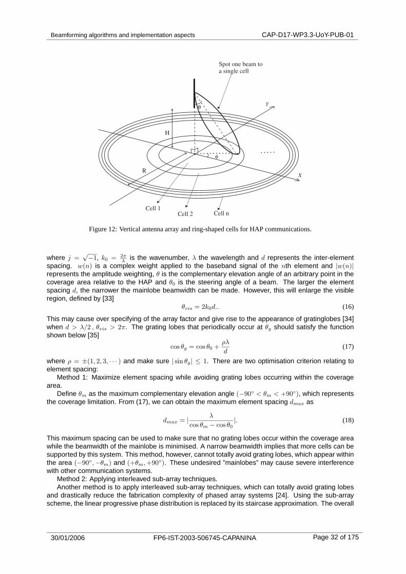
3 Vertical antenna arrays and ring-shaped cellular configurations
3.1 Introduction to ring-shaped cells and vertical antenna arrays
In the last chapter, we have proposed a method to optimize the beampattern of planar antenna array.The main advantage of this method is that one can generate a footprint with any geometry shape andstill maintain relatively low sidelobe levels. The shape of the footprint should correspond to the shapeof one cell on the ground. In the last chapter, we applied the traditional tesselating hexagonal cellularconfiguration, which means we aim to generate individual cell footprints with circular shape and equalsize. Although we have indicated that this method can lead to a reduced system payload comparedwith the solution of using a set of distinct aperture antennas, there are still several points requiringimprovement.
Firstly, generating footprints which are perfectly circular at arbitrary positions on the ground, espe-cially towards the edge of the coverage area, is extremely difficult. Some cells are not perfectly coveredby their corresponding footprints, which will cause co-channel interference and deteriorate system ca-pacity.
Secondly, sidelobe levels of the beampattern steered at the edge of coverage are about -39 dB. Thisis worse than the case when beampattern is steered at center position, where sidelobes are about -67dB. Sidelobes could be further suppressed by adjusting the parameters of the Gaussian masking filter.This process, however, can make the size of the footprint significantly larger than the correspondingcell. These disadvantages result in the requirement of considerably more antenna elements than fora set of aperture antennas [21] in order to achieve the same capacity. Since the optimized beampat-tern should serve the cellular configuration on the ground, we aim to find another cellular configurationwhere cells can be more efficiently covered from a HAP. Recently a novel ring-shaped cell configurationhas been proposed in [28] for HAP communications. Multibeams generated by a 2-dimensional rect-angular planar array are employed to provide coverage for a set of concentric ring-shaped cells on theground. Such cellular structures require no rotational motion monitoring and corrections as the HAPmoves, as well as minimizing the traffic resulting from location updating. Other major advantages lie inpower reduction and allowing the implementation of TDMA techniques, which cannot be implementedwhen applying hexagonal cellular configurations [29], [30]. However, the method has high complexity,a problem exacerbated by the relatively high large of elements required in the 2D array to achieve thedesired beampatterns.
In this chapter, ring-shaped cells are used and we propose to use a HAP-based vertical (1D) an-tenna array. We apply an interleaved sub-array structure to generate ring-shaped beampatterns toperfectly cover cells; this avoids applying complex footprint optimization techniques [31], [1] and simpli-fies the optimum weighting design process. This one-dimensional antenna approach shows a reductionof both antenna payload and implementation complexity compared with both planar antenna array andaperture antennas. Furthermore, an improvement in coverage performance has been achieved. Thischapter is organized as follows. In Section 2, the system model is described. Section 3 describes analgorithm to determine the number and sizes of cells that can be supported. Numerical results aregiven in Section 4 and finally, conclusions are given in Section 5.
3.2 System model
Fig. 12 illustrates a communication scenario with a HAP at an altitude of H (km) providing coverageover a circular area with radius of R (km). This coverage area is divided into n ring-shaped cells in orderto achieve efficient spectral re-use.
Consider a linear antenna array with N elements. The array factor of such an antenna is givenby [32]
F (θ) =
N−1∑
u=0
w(n)ejk0udcosθ (14)
andw(n) = |w(n)|e−jk0udcosθ0 (15)
30/01/2006 FP6-IST-2003-506745-CAPANINA Page 31 of 175
Beamforming algorithms and implementation aspects CAP-D17-WP3.3-UoY-PUB-01
φ
θ
X
Y
R
H
Cell 1Cell 2 Cell n
Spot one beam toa single cell
Figure 12: Vertical antenna array and ring-shaped cells forHAP communications.
where j =√−1, k0 = 2π
λ is the wavenumber, λ the wavelength and d represents the inter-elementspacing. w(n) is a complex weight applied to the baseband signal of the nth element and |w(n)|represents the amplitude weighting, θ is the complementary elevation angle of an arbitrary point in thecoverage area relative to the HAP and θ0 is the steering angle of a beam. The larger the elementspacing d, the narrower the mainlobe beamwidth can be made. However, this will enlarge the visibleregion, defined by [33]
θvis = 2k0d.. (16)
This may cause over specifying of the array factor and give rise to the appearance of gratinglobes [34]when d > λ/2 , θvis > 2π. The grating lobes that periodically occur at θg should satisfy the functionshown below [35]
cos θg = cos θ0 +ρλ
d(17)
where ρ = ±(1, 2, 3, · · · ) and make sure | sin θg| ≤ 1. There are two optimisation criterion relating toelement spacing:
Method 1: Maximize element spacing while avoiding grating lobes occurring within the coveragearea.
Define θm as the maximum complementary elevation angle (−90 < θm < +90), which representsthe coverage limitation. From (17), we can obtain the maximum element spacing dmax as
dmax = | λ
cos θm − cos θ0|. (18)
This maximum spacing can be used to make sure that no grating lobes occur within the coverage areawhile the beamwidth of the mainlobe is minimised. A narrow beamwidth implies that more cells can besupported by this system. This method, however, cannot totally avoid grating lobes, which appear withinthe area (−90,−θm) and (+θm,+90). These undesired ”mainlobes” may cause severe interferencewith other communication systems.
Method 2: Applying interleaved sub-array techniques.Another method is to apply interleaved sub-array techniques, which can totally avoid grating lobes
and drastically reduce the fabrication complexity of phased array systems [24]. Using the sub-arrayscheme, the linear progressive phase distribution is replaced by its staircase approximation. The overall
30/01/2006 FP6-IST-2003-506745-CAPANINA Page 32 of 175
Beamforming algorithms and implementation aspects CAP-D17-WP3.3-UoY-PUB-01
array factor is expressed as the product of two independently synthesized array factors, termed theprimary array Fpri(θ) and the secondary array Fsec(θ)
where Npri and Nsec define the number of antenna elements for primary and secondary array,respectively, |wpre| and |wsec| are the optimum amplitude weighting and dpri and dsec are their respectiveinter-element spacings. The primary array is designed to provide the required beamwidth and sidelobelevel. The number of elements in the secondary array is then set to the minimum for which the gratinglobes of Fsec receive enough suppression from Fpri. Spacings dpri and dsec can initially be defined asdpri = dsec = dmax. Then dpri should be reduced until there are no gratinglobes within the coveragearea θ ∈ (−90 , +90). Compared with Method 1, this method gives rise to a slightly wider beamwidth,which means slightly more antenna elements are required to support the same number of cells as inMethod 1.
Cellular design is another important part of this work. Cell configuration as shown in Fig.12 wasemployed here. The shape of the footprint on the ground is a cone for the first cell. Footprints of othercells are approximately circular rings. In [31], traditional hexagonal cellular configuration was applied,which requires generating equal-sized circular footprints by planar antenna array at any location on theground in order to cover cells. However, it is difficult to reshape the elliptical footprint to be circular atthe boundary of the coverage area. In the ring-shaped cellular configuration, cells can be more easilycovered by the footprints generated by a vertical antenna array. Thus complex footprint optimizationtechniques can be avoided, which significantly reduces computational complexity. In our scenario,window functions show clear sidelobe suppression for the vertical antenna array. Element spacingadjustment and the application of sub-array techniques can be applied to control the beamwidth andremove grating lobes, respectively.
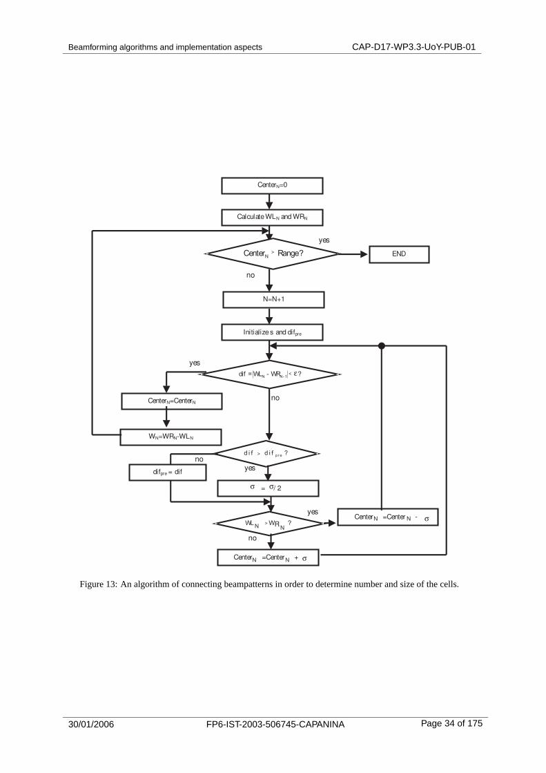
3.3 Determination of number and size of cells
Table 2: Definition of algorithmic symbolsCenterN Center position of theN th cell
WLN ,WRN Right and left boundary (defined by 3 dB beamwidth) of theN th cellWN 3dB beamwidth
Range Maximum of the coverage areadif The difference betweenWLN andWRN
difpre Previous value ofdifε An accuracy metricσ Step size
In order to analyze the coverage performance, the number and size of cells should be determined.An algorithm has been proposed to accurately define the position and width of each cell. The algorithmflow chart is shown in Fig.13 where symbol descriptions are given in Table.2. The coverage investigationmethod is similar as that employed in the last chapter.
30/01/2006 FP6-IST-2003-506745-CAPANINA Page 33 of 175
Beamforming algorithms and implementation aspects CAP-D17-WP3.3-UoY-PUB-01
yes
no
yes
no
noyes
yes
no
no
CenterN=0
CalculateWLN and WRN
CenterN=CenterN
Initialize s and difpre
WN=WRN-WLN
N=N+1
END
= / 2
Center
N
=Center +
Center =Center -
difpre = dif
>
>
> RN
N N
N N σ
σ
σ σ
< ε
Figure 13: An algorithm of connecting beampatterns in orderto determine number and size of the cells.
30/01/2006 FP6-IST-2003-506745-CAPANINA Page 34 of 175
Beamforming algorithms and implementation aspects CAP-D17-WP3.3-UoY-PUB-01
Figure 14: Comparison of the frequency response of several window functions.
3.4 Numerical results
The frequency band is selected to be 30 GHz, HAP altitude is 20 km; maximum complementary eleva-tion angle is 58.55, defining the radius of the coverage area to be 32.7 km. Different window functions- Hamming, Blackman, Chebyshev and Kaiser - have been used as the amplitude weights |w(n)|. TheHamming window can suppress the sidelobe levels down to -40 dB with the relatively narrowest beam-width. The other three windows can achieve much lower sidelobe levels. Their frequency responsesare given in Fig.14. Simulations show that using 121 antenna elements and non-subarray structure,the system can support 84 cells when applying a Hamming window and approximately 64 cells whenapplying the other three window functions.
First, array factors generated by the two methods (non-subarray and sub-array structures) are com-pared in Fig.15. For the non-subarray method, 121 elements are used and a Hamming window is ap-plied. Element spacing is 1.9λ, which is calculated by (Eq. 18) and making θb = 58.55. Grating lobesoccur at ±58.55 and ±86.98, as can be calculated by (Eq. 17). For the sub-array method, in order toachieve the same mainlobe beamwidth as the non-subarray method, 190 elements are required. Forthe primary array, there are 4 elements with element spacing 0.98λ, optimized by a Hamming window.There are 95 elements in the secondary array with 1.9λ element spacing, optimized by a Chebyshevwindow. In this case, grating lobes can be efficiently suppressed at the expense of requiring about 1.57times more antenna elements than the non-subarray method.
Next, we compare coverage performance for directive aperture antennas [1] and vertical antennaarrays using the sub-array method. In [1], 121 distinct aperture (lens) antennas are used; 4 frequencyre-use is selected and there are 30 cells for each channel. In order to compare the coverage per-formance, we select spectral re-use factor 2. Thus in our scenario, we can support 42 and 32 cells,respectively, for different window functions. Fig.16 shows coverage in the range 0.6 to 1 as a functionof SIR, which contains the most important information about coverage performance. Especially, we areinterested in the SIR values for 95% of cells. A vertical antenna array with Hamming window (H.121.42)achieves coverage performance about 5 dB better than that of a set of aperture antennas (A.121.30).And the coverage performance achieved by the other three window functions (C.121.32, B.121.32 andK.121.32) is better by up to 20 dB using the same number of antenna elements as the set of apertureantennas in [1]. However, the disadvantage is that grating lobes located outside of the coverage areamay cause interference with other communications systems. As a solution of removing grating lobes,the subarray method (S.121.42) can be applied and it can achieve performance about 9 dB better than
30/01/2006 FP6-IST-2003-506745-CAPANINA Page 35 of 175
Beamforming algorithms and implementation aspects CAP-D17-WP3.3-UoY-PUB-01
−90 −60 −30 0 30 60 90−280
−260
−240
−220
−200
−180
−160
Degree
Pow
er (
dB)
Figure 15: Comparison of the beampatterns of a vertical antenna with subarray and non-subarray structures: redline: non-subarray, 121 elems, Hamming window; blue line: subarray, 190 elems, Hamming/Chebyshev window.
30/01/2006 FP6-IST-2003-506745-CAPANINA Page 36 of 175
Beamforming algorithms and implementation aspects CAP-D17-WP3.3-UoY-PUB-01
that of the set of aperture antennas and can also support 12 more cells per channel. However, themethod requires about 1.57 times more antenna elements for one cell. As the result, considering theweight and size of the aperture antennas, our proposed vertical antenna array and ring-shaped cellu-lar configuration show advantages in both antenna payload and system complexity reduction and animprovement of coverage performance.
Further considering the proposed ring-shaped cell configuration, the size of each cell is determinedby the beamwidth of the beampatterns. The change of the beamwidth at different steering positionsresults in non-equal cell size, which increases with the distance between the cell and the coveragecenter. The boundary cell size is 28.55 km2 when Hamming windowing is applied - approximately 4.04times larger than the case for a center cell. Since the number of the users that can be supported byone cell is proportional to the cell size, this cellular configuration results in non-equal distributions ofbandwidth.
3.5 Conclusions
We have proposed using vertical antenna array and ring-shaped cellular configuration to implementcommunications from HAPs. Coverage performance has been compared with a set of 121 aperture an-tennas reported in [1]. It is shown that a non-subarray vertical antenna can achieve an improvement incoverage performance by up to 20 dB and can even support more cells for one channel with the samenumber of antenna elements compared with the set of aperture antennas. When applying subarraystructuring to the array, 1.57 times more elements are required to attenuate grating lobes and achievethe similar capacity performance. Besides the improvement of coverage performance, the vertical an-tenna solution can provide benefits in terms of implementation simplification, weight and size reduction,electrical steering flexibility and system expandability.
30/01/2006 FP6-IST-2003-506745-CAPANINA Page 37 of 175
Beamforming algorithms and implementation aspects CAP-D17-WP3.3-UoY-PUB-01
4 Array topologies for the HAP-based smart antenna
This chapter investigates the effects of antenna array topology on adaptive beamforming performancefrom high-altitude platforms, HAPs, [3] [4]. Rectangular and circular element arrangements are consid-ered for multiple-beam transmission on the HAP-Earth downlink. The signal-to-interference-plus-noiseratio (SINR) performance of the array topologies with Capon beamforming, e.g. [36] [5], is determinedin the presence of beamforming errors (HAP pitch variation), taking into account the HAP-Earth link. Itis shown that circular arrays may exhibit considerable benefits when used to implement Capon beam-forming from HAPs. In particular, antenna gain is less sensitive to the locations of interfering users,which may result, statistically, in improved performance in the presence of small beamforming errors.
Beamforming using planar rectangular arrays at mm-wave frequencies was investigated for satelliteapplications in [12] [13] and for HAPs in [14]. In [13], a satellite adaptive beamforming system wasproposed, with half-wavelength element spacing to avoid grating lobes. In [12] and [14], 4 × 4 elementarrays for adaptive beamforming were developed; the latter using 1.2λ element spacing, where 1.2λto ease problems of space for component placement in the 31/28GHz band. The problem of phaseerror in RF feeds due to unequal element feed lengths emerged in the latter work as a key hindrance tosteering calibration.
In this chapter, we investigate the performance of array topologies for adaptive beamforming ina HAP-user point-to-multipoint downlink. Rectangular and circular arrays are studied, with the aim ofestablishing constraints imposed by system performance requirements on HAP antenna array hardwaredesign. Arrays with elements spacing > 0.5λ offer increased space for component placement andreduced mutual coupling between elements; and could be beneficial at 31/28GHz, where λ ≈1 cm.Circular arrays may facilitate phase error reduction through use of radial RF feeds to elements. Thesensitivity of beamforming using the different array topologies to small uncorrected variations in HAPattitude (e.g. pitch, due to atmospheric turbulence) is presented.
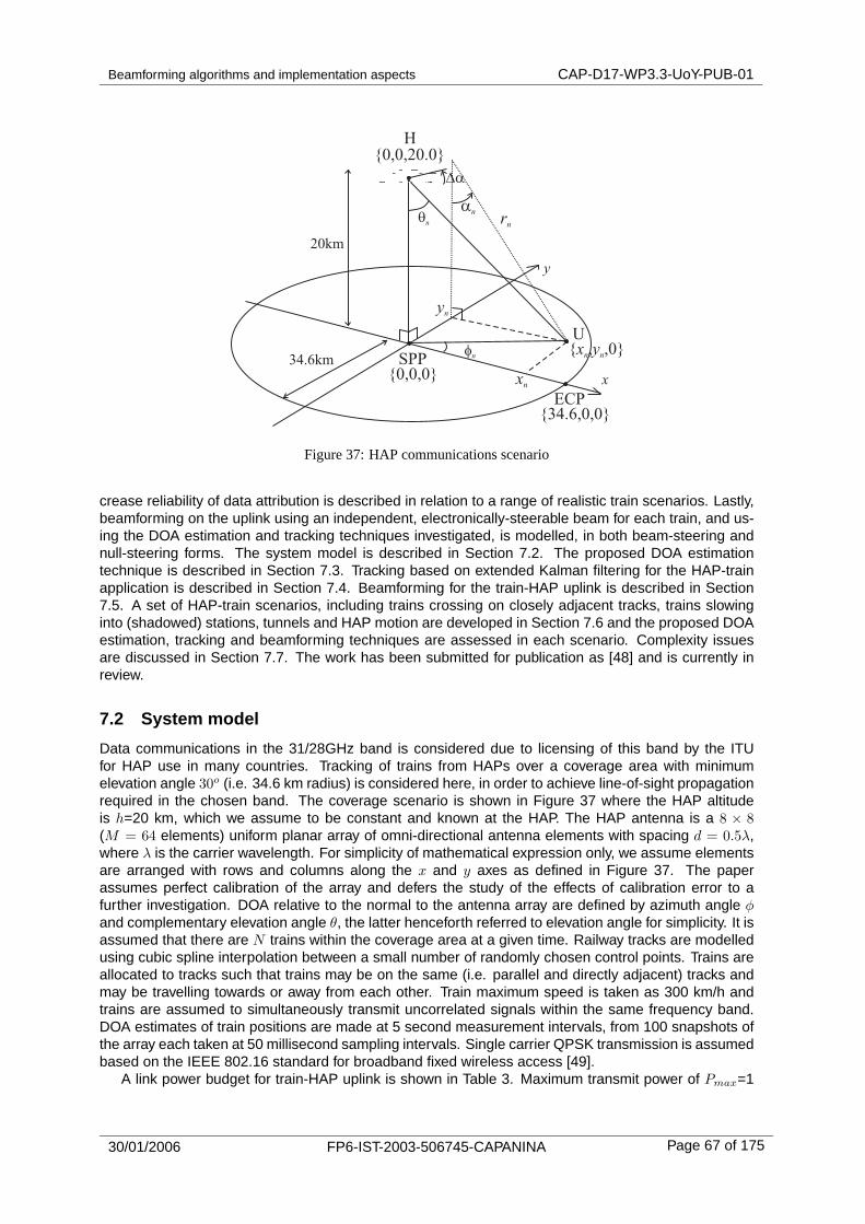
4.1 HAP communications scenario
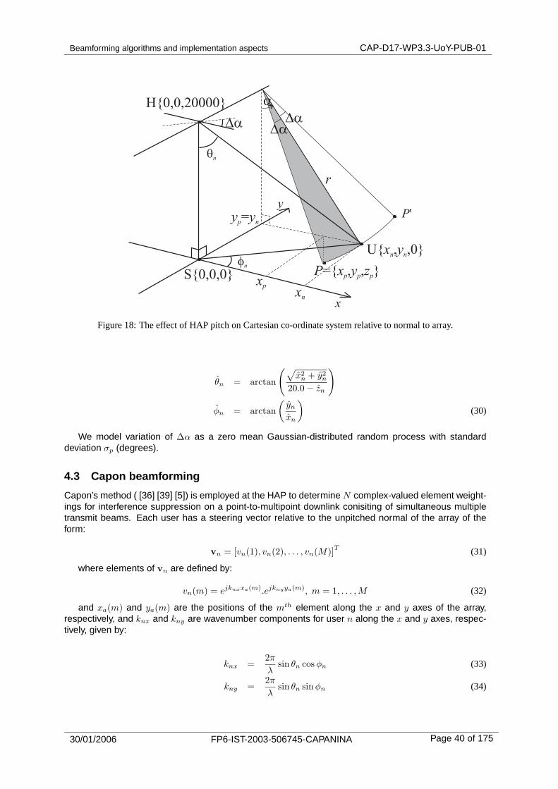
We consider the scenario in Figure 17, whereby a HAP (marked H) at altitude 20km provides coverageover an circular area with minimum elevation angle 30o. The sub-platform point (SPP), vertically belowthe HAP, and an edge of coverage point (ECP) are marked. Multiple-beam transmission on the downlink(HAP-Earth) at 28GHz from a HAP to 256 stationary users is considered. The system is assumed tohave 25 MHz bandwidth, divided into 8 time or frequency slots, such that there are N = 32 co-channelusers in the coverage area simultaneously. A HAP-mounted smart antenna with M = 64 elements isthen used to transmit 8 sets of 32 co-channel signals on 256 separate beams (i.e. 1 beam per user) onthe downlink, using Capon beamforming to spatially separate co-channel users. To evaluate the effectsof array topology alone, in the presence of only one form of error (uncorrected HAP pitch variation),we assume that the array is perfectly calibrated, that the elements are omni-directional and that thepositions of all users and the HAP are perfectly known. The antenna array is assumed to move inconjunction with the HAP.
In calculating a set of N adaptive beampatterns, it is assumed the current HAP pitch angle is notknown at the HAP; the antenna array is thus assumed to be parallel to the ground (it is assumed tobe unpitched) in the estimation of beamforming weights. Steering angles between the normal to theunpitched antenna array and each user, n, in a co-channel set are defined by the pairs:
θn, φn, n = 1, . . . , N (22)
where θn and φn are the complementary elevation angle and azimuth angle, respectively, betweenthe direction of user n and the normal to the array, as shown in Figure 17. For an array with elementsoriented in the x-y plane, θ = 0o represents the direction H-SPP and φ = 0o represents the +xdirection. If the SPP is at the origin in 3D Cartesian space, the HAP station-keeping point is located atH = 0, 0, 20.0, where values are in km, and user n is located at xn, yn, 0, then user n has steeringangles:
30/01/2006 FP6-IST-2003-506745-CAPANINA Page 38 of 175
Beamforming algorithms and implementation aspects CAP-D17-WP3.3-UoY-PUB-01
Figure 17: HAP communications scenario
θn = arctan
(√x2
n + y2n
20.0
)(23)
φn = arctan
(yn
xn
)(24)
4.2 Effect of HAP pitch
The effect of HAP pitch [37] [38] on the direction of users relative to the array normal is illustrated inFigure 18 and can be described as follows. We assume the HAP is oriented in the +x direction. TheHAP and array are jointly subject to a pitch ∆α relative to the x axis with the y axis being the axis ofpitch Figure 17. A beam steered directly at user n will move along an arc whose centre is a point onthe axis of pitch and the arc radius, rn (km), is given by:
rn =20.0
cos αn(25)
where αn is the angle of user n from the axis of pitch. Similarly, the normal to the array will movethrough angle ∆α relative to the vertical (z) axis. In the pitched co-ordinate system, the position of usern will be modified to xn, yn, zn, where:
xn = rn sin (αn − ∆α) (26)
yn = yn (27)
zn = 20.0 − rn cos (αn − ∆α) (28)
= 20.0
(1 − cos (αn − ∆α)
cos αn
)(29)
Steering angles for user n, adjusted for pitch, are then defined relative to the pitched normal to thearray as:
30/01/2006 FP6-IST-2003-506745-CAPANINA Page 39 of 175
Beamforming algorithms and implementation aspects CAP-D17-WP3.3-UoY-PUB-01
Figure 18: The effect of HAP pitch on Cartesian co-ordinate system relative to normal to array.
θn = arctan
(√x2
n + y2n
20.0 − zn
)
φn = arctan
(yn
xn
)(30)
We model variation of ∆α as a zero mean Gaussian-distributed random process with standarddeviation σp (degrees).
4.3 Capon beamforming
Capon’s method ( [36] [39] [5]) is employed at the HAP to determine N complex-valued element weight-ings for interference suppression on a point-to-multipoint downlink conisiting of simultaneous multipletransmit beams. Each user has a steering vector relative to the unpitched normal of the array of theform:
and xa(m) and ya(m) are the positions of the mth element along the x and y axes of the array,respectively, and knx and kny are wavenumber components for user n along the x and y axes, respec-tively, given by:
knx =2π
λsin θn cos φn (33)
kny =2π
λsin θn sinφn (34)
30/01/2006 FP6-IST-2003-506745-CAPANINA Page 40 of 175
Beamforming algorithms and implementation aspects CAP-D17-WP3.3-UoY-PUB-01
The set of Capon weight vectors, expressed as a set of length M column vectors, wn,n = 1, . . . ,N,are then determined by:
wn =R−1vn
vHn R−1vn
(35)
where R is the M × M spatial correlation matrix whose elements are given by:
R (m1,m2) =N∑
n=1
v∗n(m1)vn(m2) (36)
m1 = 1, . . . ,M,
m2 = 1, . . . ,M
and (.)∗ denotes conjugation. Weight vectors are normalised throughout this chapter, such that:
‖wn‖2 = 1, n = 1, . . . , N (37)
where ‖.‖2 denotes Euclidean norm.
4.4 Methodology for performance evaluation
The interference suppression capabilities of Capon beamforming are known to be strongly dependenton the angular separations of co-channel interferers (e.g. [39]). Determining the performance of thebeamforming system for an arbitrary arrangement of co-channel interferers does not provide a usefulestimate of the performance in general. Thus, a Monte Carlo approach is adopted in which a random,uniformly-distributed arrangement of N − 1 co-channel interferers is generated for each trial, and SINRis evaluated for a reference user in a fixed, worst-case position. It can be shown that this worst caseoccurs for a reference user at ECP. System performance is evaluated by the statistics (cumulativedistribution function, CDF) of SINR for the reference user.
4.4.1 Power control
We assume that the transmit power achievable from the communications payload is equal to the totalnumber of system users expressed in Watts, and that this power is distributed evenly to each set of Nco-channel users. Thus, the power output available for N users is P = N Watts. We apply power controlto ensure that differing free space path losses within each set of N co-channel users are compensated.This can be shown to achieve improved statistics of SINR. The power distribution is then defined by theset:
p(n) = PL2(n)
∑Ni=1 L2(i)
, n = 1, . . . , N (38)
where L(n) is the path length (in metres) for user n.
4.4.2 Link budget
The beampattern gain for the ith downlink beam in the direction of user n relative to the pitched arraynormal may be determined from the component of the ith beam array factor in the direction of user n,defined as:
Wi(θn, φn) =∣∣vH
n wi
∣∣2 (39)
where (.)H denotes conjugate transposition and vn is the pitched steering vector for user n whoseelements are:
30/01/2006 FP6-IST-2003-506745-CAPANINA Page 41 of 175
Beamforming algorithms and implementation aspects CAP-D17-WP3.3-UoY-PUB-01
and:
knx =2π
λsin θn cos φn (41)
kny =2π
λsin θn sin φn (42)
where θn and φn are defined in Eq. 30. Energy-per-bit Eb(n), interference-per-bit Ib(n) and noisedensity No(n), are then defined in dBs for each user using the following link budget:
Eb(n) = 10 log10
(p(n)Wn(θn, φn)
)+ η
− 20 log10
(4πL(n)
λ
)− Mrain + Gr(n) − 10 log10(Rb(n)) (43)
Ib(n) = 10 log10
N∑
i=1,i 6=n
p(i)Wi(θi, φi)
+ η
− 20 log10
(4πL(n)
λ
)− Mrain + Gr(n) − 10 log10(Rb(n))
No(n) = 10 log10(T (n)) + kdB + F (n) (44)
where η is HAP antenna efficiency (assumed to be -3dB), Mrain is a Ka-band rain margin (=3.3dBfor 99% link availability), Gr(n) are the user terminal antenna gains and Rb(n) are the user bit rates(=5Mbps assuming QPSK and 25% pulse shape filter roll-off). Noise density (dBW/Hz) is calculatedfrom Boltzmann’s constant, kdB=-228.6dBJ/K, the noise temperature of receiver, T (n) (=300K) and thereceiver noise figure, F (n) (=5dB). For simplicity, values of Gr(n), Rb(n), F (n) and T (n) are assumedto be equal for all users. A value of Gr(n)=40.9dBi is assumed equal for all users corresponding tosmall, circular aperture dishes of diameter 50cm and aperture efficiency 50%. We assume the userdishes to be perfectly pointed. We then define signal-to-noise ratio (SNR), signal-to-interference ratio(SIR) and signal-to-interference-plus-noise ratio (SINR) for user n in dB as:
SNR(n) = Eb(n) − No(n)
SIR(n) = Eb(n) − Ib(n)
SINR(n) = Eb(n) − 10 log10
(10
Ib(n)
10 + 10No(n)
10
)(45)
4.5 Array topologies
We assume signal wavelength λ = 1.07cm (f=28GHz). Figure 19 shows the three array topologiesconsidered here. Figure 19a is a square array of uniformly-spaced elements, separated by d = 0.5λbetween element centres. Figure 19b is a circular array with d = 0.5λ. Figure 19c is a square arraywith d = 1.6λ - this element spacing is chosen such that the array beampattern has the same mainlobehalf-power beamwidth (HPBW) as the circular array, as shown by the uniform element weighting beam-patterns in Figure 20. The array in Figure 19c is used to evaluate whether the performance differencespresented later between square and circular, d = 0.5λ, arrays are due to topology alone, or due to theincrease in aperture between Figure 19a and b. HPBWs for the three arrays are 12.7o (square, d = 0.5λ)and 4.0o (circular, d = 0.5λ and square, d = 1.6λ). Several key issues relate to the arrangement of an-tenna elements in smart antenna arrays. If half-wavelength spacings are employed in the 31/28GHzband to avoid grating lobes (e.g. [13]), element spacing d ≈ 0.5 cm may create problems for componentplacement. In [14], d = 1.2λ element spacing was employed to ease problems of component placementin the 31/28GHz band. In addition, mutual coupling between elements may be a problem for elementspacings of 0.5λ or less. The problem of phase error in RF feeds due to unequal element feed lengthsemerged in the work in [14] as a key hindrance to array calibration. For the arrays investigated here,
30/01/2006 FP6-IST-2003-506745-CAPANINA Page 42 of 175
Beamforming algorithms and implementation aspects CAP-D17-WP3.3-UoY-PUB-01
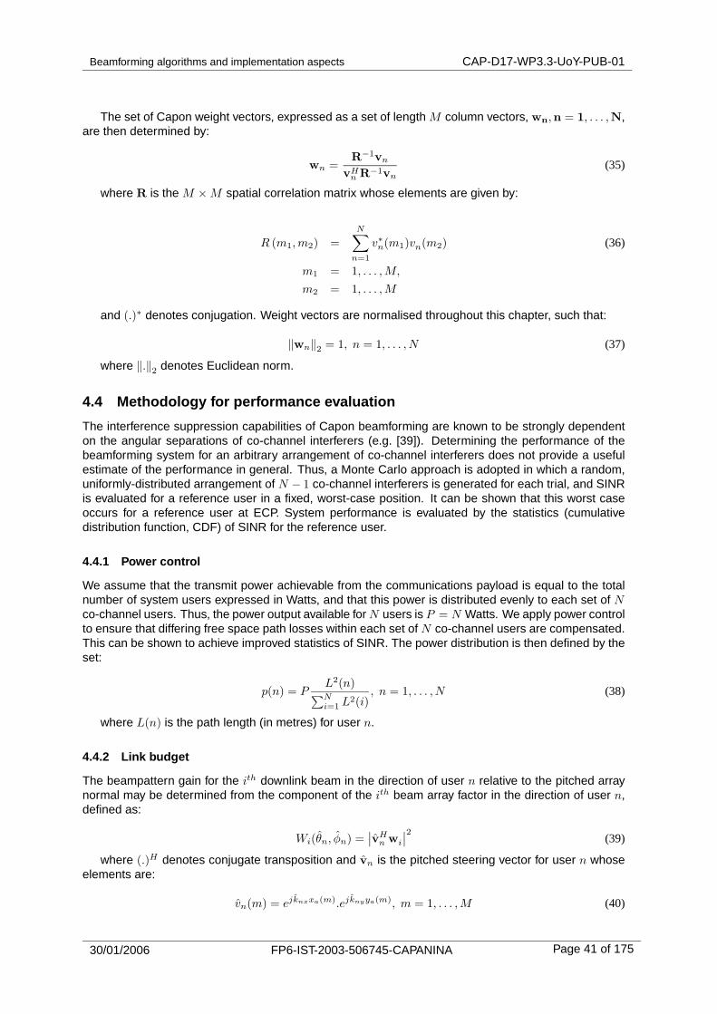
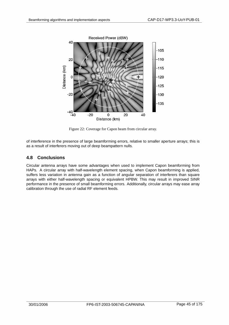
the square d = 0.5λ array is most likely to provide problems of component placement. For both squarearrays, a problem arises of how to equalise RF feed lengths to elements so as to simplify array cali-bration. Here, the circular array may provide a solution; provided that mutual coupling is small, or canbe mitigated, radial RF element feeds could be etched onto the substrate and their lengths preciselymatched to minimise phase errors. Example coverage plots of received signal power at the output ofthe user terminal antenna (dBW) are shown in Figures 21, 22 and 23 for small square (d = 0.5λ) andcircular arrays and large square (d = 0.5λ) arrays, respectively. In each case, the user beam is directedto a reference user (black cross) at ECP in the presence of 31 co-channel interferers (white crosses).With no beamforming errors, all co-channel interferers are placed in deep beampattern nulls.
−7.5−5−2.502.557.5−7.5
−5
−2.5
0
2.5
5
7.5a)
cm
cm
−7.5 −5 −2.5 0 2.5 5 7.5−7.5
−5
−2.5
0
2.5
5
7.5b)
cm−7.5 −5 −2.5 0 2.5 5 7.5
−7.5
−5
−2.5
0
2.5
5
7.5c)
cm
d=0.5λ
d=0.5λ
d=1.6λ
Figure 19: Array topologies: a) small square,d = 0.5λ, b) circular,d = 0.5λ, c) large square,d = 1.6λ.
0 10 20 30 40 50 60−20
−18
−16
−14
−12
−10
−8
−6
−4
−2
0
Elevation Angle, θ (o)
Nor
mal
ised
Dire
ctiv
ity (
dB)
Square, d=0.5λCircular, d=0.5λSquare, d=1.6λ
small square: beamwidth=12.7o
circular and large square: beamwidth=4.0o
large square: grating lobe
Figure 20: Beampatterns of three topologies through azimuth φ = 0o
4.6 Results
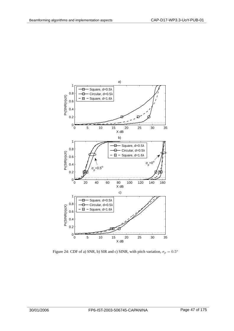
The cumulative distribution function (CDF) of SNR, SIR and SINR is presented in Figure 24a, b and c,respectively, for the three array topologies with pitch variation σp = 0.5o and 2000 Monte Carlo trials. InFigure 24a, it is shown that the circular array has, statistically, markedly improved SNR performance forlow outage probabilities; around 15dB relative to the square d = 0.5λ. array for outage probability 5%
30/01/2006 FP6-IST-2003-506745-CAPANINA Page 43 of 175
Beamforming algorithms and implementation aspects CAP-D17-WP3.3-UoY-PUB-01
Figure 21: Coverage for Capon beam from small square array.
(marked). Incidentally, the mainlobe for each array is sufficiently wide that the small pitch variation hasminimal effect on SNR. In Figure 24b, the circular and square d = 1.6λ. arrays are shown to be moresensitive to beamforming errors, due to the increased steepness of the sides of their lobes (Figure 20),resulting from larger aperture. For no pitch variation, and no other error sources, interference is almostcompletely suppressed. For CDF of SINR (Figure 24c), the circular array is shown to exhibit a markedlyhigher SINR at low outage probability than both square arrays; by approximately 7dB at 5% probability.That is, for small beamforming errors, the statistical SNR benefits of the circular array will dominate andresult in increased SINR at low outage probabilities.
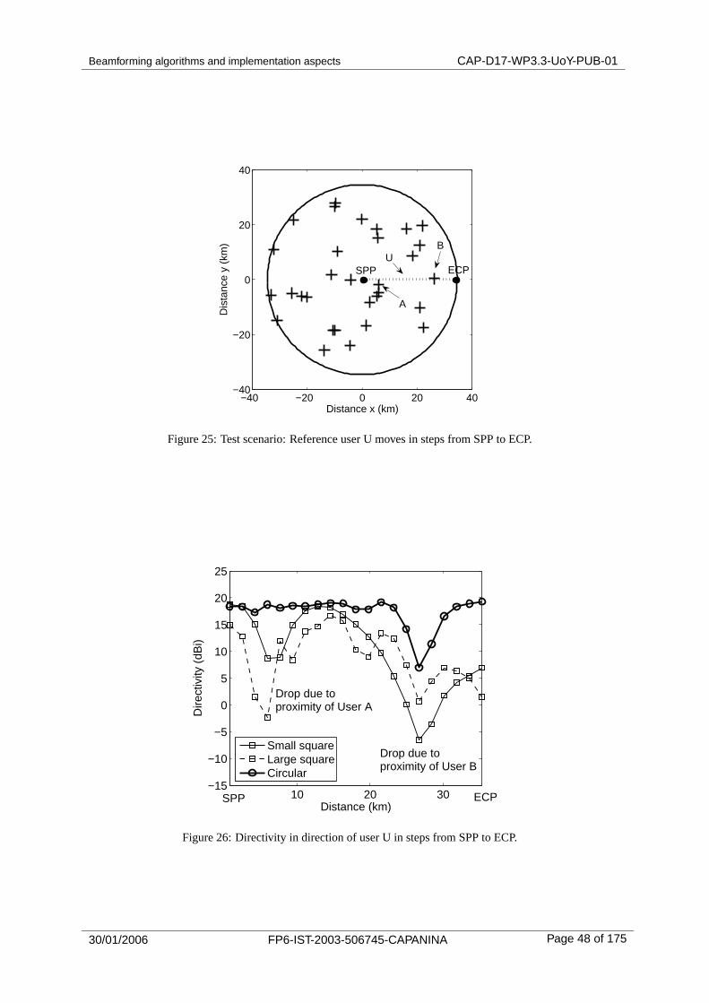
4.7 An explanation of the results
We explain the SNR benefits of the circular array as follows. In Figure 25, a test scenario is illustratedin which the reference user, U, moves in steps from SPP to ECP, through a field of 31 static interferers.In Figure 26, directivity in the direction of user U, representing a metric of useful antenna gain which inturn will affect link budget and both SNR and SINR, is plotted at each step for the three topologies withno HAP pitch variation. For small and large square arrays, sharp drops in directivity occur when thereference user is close to interferers B and C (Figure 25), due to the attempt by the Capon beamformingprocess to minimise interference. The reduction in directivity is less marked for the circular array. For alarger pitch variation of σp = 2.0o, circular and square arrays perform similarly at 5% outage probability.
To investigate the phenomenon further, we again use beampattern directivity as a measure of usefulantenna gain. Directivity is plotted in the area around the two closely spaced users in Figures 27, 28and 29 for small square, circular and large square arrays, respectively, for the case of user U placedvery close (900 metres) to co-channel user B. In all three figures, the interferer is placed in a deepbeampattern null and the key difference lies in the useful gain in the direction of the desired user. Forthe small square array, U is positioned some way down a lobe of its own beampattern, such that theuseful gain is less than 0dB. For the circular array, closer spacing of contour lines of the beampatternare noted, due to increased aperture of the array, and U is positioned close to the mainlobe of thebeampattern, receiving significant useful gain (≈10dB). For the large square array, contour lines arealso closer spaced than for the small square array, due to increased array aperture. However, althoughU is located near to a beampattern lobe, the lobe is not as prominent as for the circular array, andU receives less useful gain (≈ 5dB). It should be noted, however, that the increased steepness inbeampattern profile for the circular array, due to increased aperture, is likely to result in increased levels
30/01/2006 FP6-IST-2003-506745-CAPANINA Page 44 of 175
Beamforming algorithms and implementation aspects CAP-D17-WP3.3-UoY-PUB-01
Figure 22: Coverage for Capon beam from circular array.
of interference in the presence of large beamforming errors, relative to smaller aperture arrays; this isas a result of interferers moving out of deep beampattern nulls.
4.8 Conclusions
Circular antenna arrays have some advantages when used to implement Capon beamforming fromHAPs. A circular array with half-wavelength element spacing, when Capon beamforming is applied,suffers less variation in antenna gain as a function of angular separation of interferers than squarearrays with either half-wavelength spacing or equivalent HPBW. This may result in improved SINRperformance in the presence of small beamforming errors. Additionally, circular arrays may ease arraycalibration through the use of radial RF element feeds.
30/01/2006 FP6-IST-2003-506745-CAPANINA Page 45 of 175
Beamforming algorithms and implementation aspects CAP-D17-WP3.3-UoY-PUB-01
Figure 23: Coverage for Capon beam from large square array.
30/01/2006 FP6-IST-2003-506745-CAPANINA Page 46 of 175
Beamforming algorithms and implementation aspects CAP-D17-WP3.3-UoY-PUB-01
0 5 10 15 20 25 30 350
0.2
0.4
0.6
0.8
1
X dB
Pr(
SN
R(n
)≤X
)
a)
0 20 40 60 80 100 120 140 1600
0.2
0.4
0.6
0.8
1
X dB
Pr(
SIR
(n)≤
X)
b)
0 5 10 15 20 25 30 350
0.2
0.4
0.6
0.8
1
X dB
Pr(
SIN
R(n
)≤X
)
c)
Square, d=0.5λCircular, d=0.5λSquare, d=1.6λ
Square, d=0.5λCircular, d=0.5λSquare, d=1.6λ
Square, d=0.5λCircular, d=0.5λSquare, d=1.6λ
σp=0.5o
σp=0o
Figure 24: CDF of a) SNR, b) SIR and c) SINR, with pitch variation,σp = 0.5o
30/01/2006 FP6-IST-2003-506745-CAPANINA Page 47 of 175
Beamforming algorithms and implementation aspects CAP-D17-WP3.3-UoY-PUB-01
−40 −20 0 20 40−40
−20
0
20
40
Distance x (km)
Dis
tanc
e y
(km
)
SPP ECP
A
BU
Figure 25: Test scenario: Reference user U moves in steps from SPP to ECP.
10 20 30−15
−10
−5
0
5
10
15
20
25
Distance (km)
Dire
ctiv
ity (
dBi)
Small squareLarge squareCircular
SPP ECP
Drop due toproximity of User B
Drop due toproximity of User A
Figure 26: Directivity in direction of user U in steps from SPP to ECP.
30/01/2006 FP6-IST-2003-506745-CAPANINA Page 48 of 175
Beamforming algorithms and implementation aspects CAP-D17-WP3.3-UoY-PUB-01
−20
−20
−15
−15
−10
−10
−10
−5
−5
−5
0
0
0
5
5
5
−20
−20
−20
−15
−15
−15
−10
−10
−5
−5
−5
0
0
0
5
5
5
10
10
10
Distance (km)
Dis
tanc
e (k
m)
Directivity (dBi)
25 26 27 28 29 30
−2
−1
0
1
2
−25
−20
−15
−10
−5
0
5
10
15
20
B
U
Figure 27: Capon beampattern for small square array with U and B closely-spaced.
−20−15
−15
−15−10
−10
−10
−5
−5
−5
0
0
0
5
5
5
10
10
10
−10
−10
−10
−5
−5
−5
0
0
0
15
15
15
5
5
5
10
1015
−15−15
−20−20
−20−20
Distance (km)
Dis
tanc
e (k
m)
Directivity (dBi)
25 26 27 28 29 30
−2
−1
0
1
2
−25
−20
−15
−10
−5
0
5
10
15
20
U
B
Figure 28: Capon beampattern for circular array with U and B closely-spaced.
30/01/2006 FP6-IST-2003-506745-CAPANINA Page 49 of 175
Beamforming algorithms and implementation aspects CAP-D17-WP3.3-UoY-PUB-01
−20
−20
−20−20
−20
−20
−20−15
−15
−15
−15
−10
−10
−10
−10
−5
−5
−5
−5
0
0
0
0
5
5
5
5
1010 10
10
10
−15
−15
−15
−10
−10
−10
−5
−5
−5
00
0
0
5
5
5
15
Distance (km)
Dis
tanc
e (k
m)
Directivity (dBi)
25 26 27 28 29 30
−2
−1
0
1
2
−25
−20
−15
−10
−5
0
5
10
15
20
U
B
Figure 29: Capon beampattern for large square array with U and B closely-spaced.
30/01/2006 FP6-IST-2003-506745-CAPANINA Page 50 of 175
Beamforming algorithms and implementation aspects CAP-D17-WP3.3-UoY-PUB-01
5 Channel allocation method for adaptive beamforming from HAPs
As demonstrated in Chapter 4, the performance of smart antenna-based systems is strongly depen-dent on the spatial separation of users allocated to the same time or frequency channel. Therefore, it isimportant to consider jointly the design of channel allocation (MAC layer) and smart antenna (physicallayer) algorithms. This joint design process is sometimes referred to in the literature as space-timescheduling. The aim in space-time scheduling is typically maximisation of system throughput, for whichthe optimum method involves an exhaustive search of all possible user channel allocations. With in-creasing numbers of total users in the system (N ) and numbers of users per channel (K), this methodquickly becomes computationally prohibitively; it requires evaluation of a utility function, typically basedon signal-to-interference plus noise ratio (SINR), over all
(NK
)possible user channel allocations. Heuris-
tic approaches of lower complexity were presented initially in [9] and more recently in [10] and [11].In providing broadband coverage using a HAP-based smart antenna, with a coverage area of 70km
diameter, the number of simultaneous users is potentially very large. In the chapter, we assume thereare N=1024 total users in the coverage area, and that system bandwidth is divided into L=32 frequencyor time slots, such that there are K=32 users per channel. The elevation of the HAP allows beamformingin three dimensions (as opposed to two for terrestrial systems). This allows benefits from increasednumbers of antenna elements in the interference suppression of co-channel users, as well as helpingto mitigate the increased free space path loss. We assume as in Chapter 4 that a HAP-based smartantenna with M = 64 (8× 8) elements is used to provide interference suppression. Methods describedin [9], [10] and [11] are applicable to terrestrial base station scenarios in which the total number of usersin the system, and the number of users per channel, are relatively small. Application of these algorithmsto the HAP scenario described here leads to prohibitive computational complexity, as discussed in thenext section.
This chapter presents a novel channel allocation method at the medium access control (MAC)layer to increase the capacity enhancement that may be achievable through adaptive beamformingon point-to-multipoint links. The method allocates users to channels such that the probability of allocat-ing closely-spaced users to the same channel is significantly reduced. The technique is deterministic,based purely on the spatial separation of users, as determined either using GPS or using direction-of-arrival estimation at the HAP on the uplink. It therefore requires no search or computationally intensiveoptimisation method, and is practicable for large numbers of total users in a system and large numbersof users per channel, as experienced in a HAP (or satellite) scenario.
Spatial re-use on a point-to-multipoint downlink (base-station to multiple users), as studied here,can also be termed space division multiplexing, SDM. In this chapter, we consider a HAP-user downlinkin which SDM is applied in addition to time- or frequency-division multiplexing (TDM or FDM). We eval-uate the performance of the proposed algorithm for beamforming with a single source of beamformingerrors which is specific to the HAP scenario - that of uncorrected variations in the HAP attitude (e.g.pitch, Chapter 4). The proposed channel allocation algorithm is shown to provide substantial capacityenhancements (up to 75%) compared to arbitrary SDM-TDM or SDM-FDM allocations.
5.1 Background to channel allocation methods for smart ante nnas
Recently, in [10] and [11], the problem of downlink channel allocation for multiple antenna systems hasbeen addressed. In [10], heuristic space-time scheduling methods based on a greedy algorithm anda genetic-based algorithm were developed. Performance was compared with an exhaustive search ofall user combinations in a given slot, for 1, 2 and 4 transmit antennas and total number of users in thesystem, N , varying between 4 and 20. The lowest complexity method investigated in the paper, thegreedy algorithm, requires N evaluations of a utility function (assumed to be convex) and O(Nlog2(N))sorting operations. For N=1024 in the HAP scenario, this scheme becomes extremely computationallyintensive.
In [11], heuristic space-time scheduling based on a discrete stochastic optimization [40] was pro-posed, to facilitate throughput optimisation in conjunction with the SINR balancing method proposedin [41], which we will use in Chapter 6. The method in [11] was demonstrated for the case of a basestation with M=4 transmit antennas, N=8 total users in the system and each channel (user subset)consisting of K=4 users. The method updates a state probability estimate for all possible |θ| =
(NK
)
30/01/2006 FP6-IST-2003-506745-CAPANINA Page 51 of 175
Beamforming algorithms and implementation aspects CAP-D17-WP3.3-UoY-PUB-01
states (i.e. channel allocations) based on the SINR estimation for each state visited, and allows tran-sition to a new state (allocation) only if there is strong evidence to suggest that the state is closer toa global optimum. State probabilities for |θ| =
(102432
)= 4.97 × 1060 possible channel allocations
must be recorded, although without necessarily visiting all possible states. Again, this method is notpracticable in the HAP scenario.
5.2 Description of channel allocation method
A combined SDM-TDM or SDM-FDM downlink is considered in which system bandwidth is dividedamongst N users using L time or frequency channels. SDM is implemented by Capon beamforming,as described in Chapter 4, on groups of K = N
L users allocated to each channel. Let the user-channelallocations be expressed as an K row by L column matrix, A, where each column represents the usersassigned to the same channel. For N=8 users and L=4 channels, the matrix A before allocation wouldbe:
Chan. 1 2 3 4UserUser
The proposed algorithm is described in general in the following steps:
1. Select starting user, 1 ≤ ns ≤ N
2. Assign user ns to row 1, channel 1 of A
3. Designate this user the reference for all spatial separations in current row, or ripple centre, de-noted n0
4. Locate nearest L − 1 unallocated neighbours, n1, . . . , nL−1, to ripple centre n0
5. Assign users n1, . . . , nL−1 to current row of A in channels 2, ..., L
6. Move to next row of A
7. Assign Lth nearest neighbour, nL, relative to previous ripple centre to channel 1 of A of currentrow - this user becomes new ripple centre, n0
8. Repeat stages 4 to 7 until A is filled
We continue the simple example for N = 8 users and L = 4 channels, and denote the N users eachby a number 1, . . . , N . An example distribution of users in the coverage area is shown in Figure 31a. Auser is selected at random as a start user, ns; here we choose ns=1. The L − 1 nearest neighbours tons, in this case users 6, 4 and 3, are selected and allocated across the channels of the first row of A.The Lth nearest neighbour, in this case user 8, becomes the centre of a new ripple, and the nearestunallocated users, in this case users 2, 7 and 5 are allocated across the next row of A, as shown inFigure 31b. The contents of matrix A after channel allocations, for the example shown, would be:
Chan. 1 2 3 4User 1 6 4 3User 8 2 7 5
The method is deterministic and can be used to generate good mappings of users to channels evenfor large numbers of users and channels, with no time-consuming search algorithms, as illustrated inthe following sections.
30/01/2006 FP6-IST-2003-506745-CAPANINA Page 52 of 175
Beamforming algorithms and implementation aspects CAP-D17-WP3.3-UoY-PUB-01
Figure 30: HAP communications scenario
5.3 Application of channel allocation method to HAP communi cations scenario
We now consider larger numbers of users and channels in a scenario in which beamforming fromHAPs is performed to fixed users. The scenario is identical to that described in Chapter 4, for which thescenario diagram is repeated as Figure 30 for convenience.
We consider a case in which we wish to serve at least N = 1024 users in a SDM-TDM or SDM-FDM downlink. We consider the system bandwidth divided in L = 32 channels. A HAP-based smartantenna with M = 64 (8 × 8) elements is used to provide SDM. This smart antenna can serve thenecessary number of users per channel (K=32) at half the spatial re-use limit for the antenna (K=64).This allows a margin to be designed into the system, to compensate for beamforming errors. A MonteCarlo approach is employed in which a random positional distribution of N=1024 users within the HAPcoverage area is generated for each trial. Both a random channel allocation of users within A and theproposed method described above are applied to the users over L = 32 channels.
5.3.1 Effect of channel allocation method on distances betw een co-channel users
The cumulative distribution function (CDF) of the spatial separation in km, Ds, between all combinationsof pairs of users allocated to the same channel (i.e. users in the same column of A) in the scenariodescribed above is plotted in Figure 32, for the random and proposed methods with 2000 Monte Carlotrials. That is, each trial consists of evaluation of channel allocation matrix A followed by evaluation ofCDF of distances between all pairs of users allocated the same channel. It is shown that the proposedalgorithm reduces, compared to a random allocation, the probability of co-channel users being locatedwithin a few km, even when the total number of users is increased by 75% to N=1792. In the followingsections, we will evaluate the impact of the proposed algorithm on beamforming performance.
5.3.2 Methodology for beamforming performance evaluation
We apply a performance methodology similar to that used in Chapter 4. A Monte Carlo approachis used in which each trial represents a random distribution of co-channel interferers within a HAPcoverage area. The proposed channel allocation method is applied to the distribution of users at eachtrial. Capon beamforming is applied to that channel which contains a reference user at an edge ofcoverage point (worst case scenario). Signal-to-interference ratio (SIR) is evaluated for the reference
30/01/2006 FP6-IST-2003-506745-CAPANINA Page 53 of 175
Beamforming algorithms and implementation aspects CAP-D17-WP3.3-UoY-PUB-01
−40 −20 0 20 40−40
−20
0
20
40a)
x (km)
y (k
m)
−40 −20 0 20 40−40
−20
0
20
40b)
x (km)
y (k
m)
13
46
8 5 8 2
7
Figure 31: Allocation of users across channels in a) first rowand b) second row ofA
Figure 32: CDF of pairwise separationDs (km) of co-channel users
user. Beamforming errors are modelled again using a zero-mean, Gaussian-distributed random HAPpitch variation (Section 4.2) with standard deviation σp = 0.33o. Element spacing is d = 0.5λ.
5.3.3 Effect of channel allocation method on SIR of users
The CDF of SIR is shown in Figure 33 for a reference user at edge of coverage point ECP. A probabilityof outage (SIR < X(dB)) of 5% is chosen as an acceptable performance benchmark for the HAPcommunications system; this value is marked as a dashed horizontal line on the CDF plot. It is shownthat system capacity may be increased by up to 75% for the benchmark outage probability. A furtherbenefit of the algorithm is that by selecting a different starting user, 1 ≤ ns ≤ N , a different channelallocation A is achieved. Thus by changing allocations at regular intervals, the likelihood of a specificuser remaining in the tail of the SIR distribution for an extended period of time is reduced.
30/01/2006 FP6-IST-2003-506745-CAPANINA Page 54 of 175
Beamforming algorithms and implementation aspects CAP-D17-WP3.3-UoY-PUB-01
Figure 33: CDF of SIR for reference user with random and proposed channel allocations.
30/01/2006 FP6-IST-2003-506745-CAPANINA Page 55 of 175
Beamforming algorithms and implementation aspects CAP-D17-WP3.3-UoY-PUB-01
5.4 Conclusions
The chapter has described a channel allocation method which can be applied to the space-time schedul-ing problem - efficiently allocation of users across joint spatial- and time-separated channels - in a HAPscenario. The HAP scenario differs from the terrestrial scenario typically assumed in the design ofspace-time scheduling algorithms; the large number of simultaneous users in a HAP coverage area(100’s or 1000’s) prohibits the use of exhaustive searches for optimal channel allocations and subop-timal strategies proposed in the literature for terrestrial base-stations. The method proposed here isbased purely on the spatial distrbution of the users in the coverage area, is fast, deterministic andyields capacity improvements of up to 75% relative to random channel assignments, in the presence ofnon-Gaussian element phase errors (e.g. HAP attitudinal variation).
30/01/2006 FP6-IST-2003-506745-CAPANINA Page 56 of 175
Beamforming algorithms and implementation aspects CAP-D17-WP3.3-UoY-PUB-01
6 SINR balancing for the HAP-user downlink
Consider the case of a base station equipped with a smart antenna to achieve spatial re-use of band-width within a coverage area or cell. Signal-to-interference-plus-noise ratio (SINR) at the base stationon the uplink (user terminal to base station), for each user channel, is an independent function of eachuser adaptive beampattern, along with the relative transmit powers and distances of the user terminals.However, on the downlink the SINR at each user terminal is a function of all the adaptive beampatternsgenerated for all co-channel users. In Chapter 4, we considered the case where a set of user beamswere generated independently using Capon’s method for a set of stationary users within a HAP cover-age area. In this chapter, we investigate whether better performance can be achieved, in terms of userSINR on the downlink, by jointly estimating adaptive antenna weightings and transmit powers across allusers within a coverage area.
The problem of determining optimal user transmit powers for downlink beamforming using smartantennas was first addressed in [42]. The problem has recently been extended to the case of jointestimation of both optimum power levels and weight vectors to balance user SINR according to setof constraints [41]. The method in [41] is based on eigen-decomposition of a matrix representing thecross-coupling between the adaptive user beams. The method allows, in the case of equal user datarates and therefore equal required SINR, the balancing of user SINRs within a cell. We investigatethe method in [41] for use in the HAP broadband communication scenario presented in Chapter 4, andcompare the performance with independently-estimated Capon user beams, with and without powercontrol. The HAP-Earth link budget and likely numbers and distributions of user terminals are takeninto account. It is shown that balancing of user SINR can potentially yield improved SINR in a HAPcommunications scenario provided that a suitable channel allocation algorithm, such as that describedin Chapter 5, is applied prior to beamforming. This latter condition ensures that user SINRs are notbalanced to a low value.
6.1 Description of Schubert and Boche method
This section describes the method in [41] proposed for solving the problem of joint estimation of weightvectors and transmit powers on a multi-antenna downlink so as to meet a set of user SINR constraints.Consider a point-to-multipoint scenario in which there are N users within a coverage area or cell, withassociated minimum SINR values, γ1, . . . , γN . The total transmit power available at the base station islimited to Pmax. We define a set of complex antenna element weight vectors for the N users on thedownlink, denoted for convenience by an M row by N column matrix, U = [u1, . . . ,uN ], where M is thenumber of elements in the antenna array. We assume throughout this chapter that each user weightvector is normalised such that ‖un‖2 = 1, 1 ≤ n ≤ N . We define a set of M × M downlink spatialcovariance matrices Rn, 1 ≤ n ≤ N for the users, whose elements are given by:
Rn = vnvHn (46)
where vn ∈ CM is the steering vector associated with user n. We assume reciprocity in the uplink
and downlink, an assumption justified in a time division duplex (TDD) system. SINRs for the user nchannel on the uplink and downlink, respectively, are then represented by the two expressions:
SINRUL(n) (un,q) =q(n)uH
n Rnu(n)
uHn
(∑Km=1,m 6=n q(m)Rm + σ2
nI)un
(47)
SINRDL(n) (U,p) =p(n)uH
n Rnun∑Nm=1,m 6=n p(m)uH
n Rmun + σ2n
(48)
where q(n) and p(n) denote uplink and downlink transmit powers, respectively, for user n and σ2n
denotes the noise variance of the nth user channel.
30/01/2006 FP6-IST-2003-506745-CAPANINA Page 57 of 175
Beamforming algorithms and implementation aspects CAP-D17-WP3.3-UoY-PUB-01
6.1.1 Optimisation of power assignment for SINR balancing
The SINR balancing problem with power control on the uplink or downlink can then be described by asearch for the SINR balanced levels:
CUL (U, Pmax) = maxq
min1≤n≤N
SINRUL(n) (un,q)
γn, (49)
subject to ‖q‖1 ≤ Pmax
CDL (U, Pmax) = maxp
min1≤n≤N
SINRDL(n) (U,p)
γn, (50)
subject to ‖p‖1 ≤ Pmax
It was shown in [42] and [41] that the solutions to the balancing problems in Eqs. 49 and 50 aregiven by:
CUL (U, Pmax) =1
λmax (Λ(U, Pmax))(51)
CDL (U, Pmax) =1
λmax (Υ(U, Pmax))(52)
(53)
where λmax(.) denotes maximal eigenvalue and:
Λ(U, Pmax) =
[DΦT (U) Dσ
1Pmax
1T DΦT (U) 1Pmax
1T Dσ
](54)
Υ(U, Pmax) =
[DΦ(U) Dσ
1Pmax
1T DΦ(U) 1Pmax
1T Dσ
](55)
(56)
define extended coupling matrices on the uplink and downlink, respectively, where coupling betweenusers is defined by the matrix Φ which is a function of U:
[Φ (U)]mn =
uH
n Rmun n 6= m
0 n = m(57)
and σ =[σ2
1 , . . . , σ2N
]Tand D = diag
(γ1/
(uH
n Rnun
), . . . , γN/
(uH
NRNuN
)). In conclusion,
Schubert and Boche showed that the power assignment problem (i.e. disregarding initially the problemof optimised weight vector assignment) could be expressed in terms of the following two eigen-systemsfor the uplink and downlink, respectively:
Λ(U, Pmax)qext = λmax (Λ(U, Pmax)) qext (58)
Υ(U, Pmax)pext =1
CDL(U, Pmax)pext (59)
(60)
where pext =(p
1)
and qext =(q
1)
6.1.2 Joint optimisation of power assignment and weight vec tor for SINR balancing
Schubert and Boche then extended this SINR balancing to take into account not only optimum powerassignment but also the optimum weight vector set to achieve balanced SINR. They first redefined the
30/01/2006 FP6-IST-2003-506745-CAPANINA Page 58 of 175
Beamforming algorithms and implementation aspects CAP-D17-WP3.3-UoY-PUB-01
optimisation problem as:
CDLopt (Pmax) = max
U,pmin
1≤n≤N
SINRDL(n) (u,p)
γn, (61)
subject to ‖p‖1 ≤ Pmax
‖u‖2 = 1, 1 ≤ n ≤ N
(62)
The joint optimisation problem was then reduced to a set of K decoupled problems, thus:
un = arg maxun
uHn Rnun
uHn Qn(qext)un
, s.t. ‖un‖2 = 1,∀n (63)
where
Qn(qext) =
K∑
m=1,m 6=n
[qext]m Rm + I, ∀n (64)
where Rn = Rn/σ2n. The solution to Eq. 63, for each user, is found by taking the dominant gener-
alised eigenvector for each matrix pair (Rn,Qn(qext)), 1 ≤ n ≤ N . An iterative algorithm for solvingthe joint optimised downlink was then proposed, using iterative solution of the equivalent uplink definedby the following steps:
11. compute the downlink power allocation popt by solving:
Υ(U(k), Pmax)
[popt
1
]= λmax(k)
[popt
1
]
As in the original paper ( [41]), it was found in this work that three iterations of the SINR balancingalgorithm above were sufficient to provide a high degree of SINR balancing. Three iterations will beassumed throughout the remainder of this section.
30/01/2006 FP6-IST-2003-506745-CAPANINA Page 59 of 175
Beamforming algorithms and implementation aspects CAP-D17-WP3.3-UoY-PUB-01
6.2 Complexity
Step 6) requires a generalised eigendecomposition of M × M matrices for each user and for eachiteration. Step 8) requires a eigendecomposition of the N + 1 × N + 1 extended coupling matrix for foreach iteration only. Step 11) requires a single eigendecomposition of the (N + 1) × (N + 1) extendedcoupling matrix. Thus step 6) can be said to dominate complexity, and is O(NM3) per iteration. Incomparison, complexity for the case of individually estimated Capon beam is O(NM3) (non-iterative).We can conclude that the SINR balanced downlink carries approximately three-times the complexity ofa Capon beamforming downlink.
6.3 Application of SINR balancing to the HAP scenario
The SINR balancing method of Schubert and Boche was applied to the HAP broadband communica-tions scenario developed in Chapter 4, in order to compare with performance of a system with inde-pendently estimated powers and Capon beams for each user. The SINR balancing method requiresestimates of the user covariance matrices to be scaled according to the noise variances of the users,step 2). In practice, this could be achieved at the HAP by the following steps:
1. Perform DOA estimation at the HAP to determine user positions, x(n), y(n), n = 1, . . . , N wherevalues are in km)
2. Use 1) to estimate user path lengths, L(n), n = 1, . . . , N
3. Estimate user steering vectors
4. Use 2) to estimate user covariance matrices
5. Apply link budget knowledge and 2) to estimate scaled noise variances of users
6. Use user covariance matrices and noise variances to perform SINR balancing
To simplify the analysis, we assume in the remainder of this Chapter that DOA estimation in step 1)is perfect. The impact of DOA estimation errors in HAP-based smart antenna communications will beinvestigated in detail in Chapter 7. Path lengths L(n) in 2) are calculated by:
L(n) =√
x2(n) + y2(n) + h, n = 1, . . . , N (65)
For Capon’s method with power control, which we will use as a benchmark later, transmit power isassigned to users at the HAP so as to compensate for differing path lengths, and therefore free-spacepath losses, of the users, thus:
p(n) = PmaxL2(n)
∑Nm=1 L2(m)
, n = 1, . . . , N (66)
Note that in the SINR balancing method, this step is not required, as power levels are evaluated instep 11) of the SINR balancing method algorithmic description. For SINR balancing, the link budgetfrom Chapter 4 is required to determine relative scalings of user covariance matrices and user noisevariances in step 5). Specifically, we define a total channel gain defined by:
Gtotal = 20 log10
(4πL(n)
λ
)− Mrain + Gr(n) − 10 log10(Rb(n)) (67)
where, as in Chapter 4, Mrain is a Ka-band rain margin (=3.3dB for 99% link availability), Gr(n) arethe user terminal antenna gains and Rb(n) are the user bit rates (=5Mbps assuming QPSK and 25%pulse shape filter roll-off). Correct scaling of noise variances relative to covariance matrices for SINRbalancing in terms of energy per bit to noise density plus interference per bit ratio is then achieved by:
σ2n = 10 log10(T (n)) + kdB + F (n) − Gtotal (68)
30/01/2006 FP6-IST-2003-506745-CAPANINA Page 60 of 175
Beamforming algorithms and implementation aspects CAP-D17-WP3.3-UoY-PUB-01
where kdB=-228.6dBJ/K is Boltzmann’s constant, the noise temperature of receiver, T (n) = 300Kand the receiver noise figure, F (n) = 5dB. For simplicity, values of Gr(n), Rb(n), F (n) and T (n) areassumed to be equal for all users. A value of Gr(n)=40.9dBi is assumed equal for all users correspond-ing to small, circular aperture dishes of diameter 50cm and aperture efficiency 50%. We assume theuser dishes to be perfectly pointed. These values are the same as those used in Chapter 4. The resultsin Eq. 68 are used in step 2) of the SINR balancing method. Complex beamforming element weightsare calculated as the set U = [u1, . . . ,uN ] using the SINR balancing method, with Capon’s method(Chapter 4) used as a benchmark. Actual SINR is calculated using:
Eb(n) = 10 log10
(p(n)uH
n Rnun
)
− 20 log10
(4πL(n)
λ
)− Mrain + Gr(n) − 10 log10(Rb(n)) (69)
Ib(n) = 10 log10
N∑
m=1,m 6=n
p(m)uHmRnum
− 20 log10
(4πL(n)
λ
)− Mrain + Gr(n) − 10 log10(Rb(n))
No(n) = 10 log10(T (n)) + kdB + F (n)
SINRactual(n) = Eb(n) − 10 log10
(10
Ib(n)
10 + 10No(n)
10
)(70)
6.4 Importance of effective channel allocation
We now demonstrate the effect of the distribution of users within the HAP coverage area on user SINRfor independently estimated Capon beams with power control and the SINR balancing method proposedby Schubert and Boche. To simplify the analysis, we begin by assuming no attudinal HAP variations orother beamforming errors. Two randomly-generated user distributions of 8 co-channel users, numbered1 to 8, are shown in Figure 34 a) and b). In a), users are well spaced whilst in b), users 2 and 5 areat once closely spaced, at the edge of the coverage area and approximately in line with the HAP. Allthree factors in the latter case will lead to difficulty in spatial separation using beamforming techniques.Actual user SINRs in Eq. 70) for the cases in Figure 34 a) and b) are plotted in Figure 34 c) and d),respectively, for independently-generated Capon user beams with power control. For the distributionin a), user SINRs are approximately equal (≈15dB), because the varying HAP-user path lengths havebeen compensated for in the power control. However, for the distribution in b), users 2 and 5 havemuch lower SINR (<0dB) due to reduction in useful user gain (directivity) when interferers are close toa desired user (Chapter 4).
30/01/2006 FP6-IST-2003-506745-CAPANINA Page 61 of 175
Beamforming algorithms and implementation aspects CAP-D17-WP3.3-UoY-PUB-01
a)−40 −20 0 20 40
−40
−20
0
20
40
1
2
3
4
5
6
7
8
Distance x (km)
Dis
tanc
e y
(km
)
b)−40 −20 0 20 40
−40
−20
0
20
40
1
2
3
4
56
7
8
Distance x (km)
Dis
tanc
e y
(km
)
c)1 2 3 4 5 6 7 8
0
2
4
6
8
10
12
14
16
18
20
SIN
R (
dB)
User d)1 2 3 4 5 6 7 8
0
2
4
6
8
10
12
14
16
18
20
SIN
R (
dB)
User
Figure 34: a) Favourable user distribution, b) less-favourable user distribution of 8 users, c) User SINRs forCapon’s method with power control with favourable distribution, d) User SINRs for Capon’s method with powercontrol with less-favourable distribution
30/01/2006 FP6-IST-2003-506745-CAPANINA Page 62 of 175
Beamforming algorithms and implementation aspects CAP-D17-WP3.3-UoY-PUB-01
In Figure a) and b), user SINR is plotted for the SINR balancing method for the user distributions inFigure 34a) and b), respectively. For the favourable user distribution in Figure 34a), the SINR balancingmethod successfully equalises user SINR at 15.3dB. For the less-favourable user distribution in Figure34 b), SINR are again equalised, but this time to a much lower level (3.8dB). The benefits, or otherwise,of SINR balancing are evaluated further by a Monte Carlo approach in the next section.
a)1 2 3 4 5 6 7 8
0
2
4
6
8
10
12
14
16
18
20
SIN
R (
dB)
User b)1 2 3 4 5 6 7 8
0
2
4
6
8
10
12
14
16
18
20
SIN
R (
dB)
User
Figure 35: a) User SINRs for SINR-balancing with favourabledistribution, d) User SINRs for SINR-balancingwith less-favourable distribution
30/01/2006 FP6-IST-2003-506745-CAPANINA Page 63 of 175
Beamforming algorithms and implementation aspects CAP-D17-WP3.3-UoY-PUB-01
6.5 Monte Carlo performance study
In this section, we investigate whether the SINR balancing method could have real benefits in a HAPcommunications scenario. This investigation is performed through a Monte Carlo analysis. A cumulativedensity function (CDF) of actual SINR for a single reference user at the edge of coverage is plotted inFigure 36 for 500 Monte Carlo trials. The HAP-based smart antenna consists of 64 (8×8) elements in aplanar array. It is assumed that there are 128 users in the coverage area and 4 time- of frequency chan-nels are available within the system. As in Chapter 4, each trial consists of a random uniform distributionof all users in the coverage area. Random channel allocation and the method proposed in Chapter 5are used, as indicated on the graph. Zero mean, Gaussian HAP pitch variations with standard deviation0.33o (Chapter 4) are used as the single source of beamforming errors. For both methods of channelallocation the benefit of using power control in the Capon method are shown - statistics of SINR areimproved. As in Chapter 4, we again use 5% outage probability as a benchmark for acceptabe perfor-mance, as marked by the dashed line. For the random allocation, SINR balancing leads to worse SINR,statistically, at the benchmark level than independently-estimated Capon beamforming with power con-trol; SINR is often balanced to a very low level when interferers are close to the desired user. When thechannel allocation method proposed in 5 is used, SINR balancing leads to improved performance byapproximately 3dB at 5% outage probabilitycompared to independently-estimated Capon beamformingwith power control; likelihood of interferers close to the desired user being allocated to the same time-or frequency channel as the desired user has been significantly reduced. As a result, SINR balancinghas lead, statistically, to higher SINR and can be said to be of some benefit in adaptive beamformingfrom HAPs.
Capon, no power controlCapon, power controlEqualised SINR
random channelallocation
proposed channel allocation
Figure 36: HAP communications scenario
30/01/2006 FP6-IST-2003-506745-CAPANINA Page 64 of 175
Beamforming algorithms and implementation aspects CAP-D17-WP3.3-UoY-PUB-01
6.6 Conclusions
In this chapter, the use of SINR balancing in the HAP communications scenario is investigated. Aniterative eigendecomposition-based algorithm which jointly estimates transmit power levels and weightvectors so as to balance SINR for a set of users is applied to the adaptive beamforming HAP downlink.It is shown that SINR balancing can be beneficial in the scenario, reducing the probability of very lowSINR for some users. However, this is only the case when used in conjunction with a channel allocationalgorithm which can reduce the probability of closely-spaced users being allocated the same time- orfrequency-channel. At 5% outage probability, SINR is increased by ≈ 3dB using the SINR-balancingmethod in conjunction with the proposed channel allocation scheme from Chapter 5 Computationalcomplexity is approximately three times that associated with individually-optimised Capon beams.
30/01/2006 FP6-IST-2003-506745-CAPANINA Page 65 of 175
Beamforming algorithms and implementation aspects CAP-D17-WP3.3-UoY-PUB-01
7 Data communications to railway trains from HAPs
In this chapter, signal processing techniques for providing simultaneous high data-rate communicationlinks to multiple moving railway trains from high-altitude platforms (HAPs) using a ’smart’ antenna arrayare investigated. Techniques for estimation of the number of trains present, accurate direction-of-arrival(DOA) estimation and tracking of multiple trains for the purposes of beamforming and reliable attri-bution of DOA estimates to trains are studied in a range of train scenarios, including trains crossingand passing through tunnels and stations. It is shown that extended Kalman filtering (EKF), in addi-tion to providing improved accuracy of positional estimation of trains, particularly when they cross orpass closely, also ensures reliable attribution of DOA estimates to trains. Methods for adapting EKFfor tracking trains passing through tunnels and shadowed stations are proposed and it is shown thattracking can be initialised so as to cope with both slow variations in train velocity and sudden HAP mo-tion. Beamforming based on null-steering is shown to be beneficial in HAP-train data communicationseven for small numbers of trains; providing increased stability of signal-to-interference-plus-noise ratio.Based on the findings, a suite of array signal processing techniques is developed based on an iterativeroot-MUSIC DOA method, extended Kalman tracking and Capon beamforming.
Provision of high data rate services to train travellers has been a topic of much recent researchinterest [16] [17], resulting in the emergence of internet access based on wireless local area networks(WLANs) on some commercial train routes, e.g. [18] [19]. Existing services are typically realised us-ing a combination of geostationary satellite and terrestrial cellular links; satellite links being used toprovide higher speed connections where line-of-sight to geostationary earth orbiting (GEO) satellitesis available, whilst multiple terrestrial cellular links are often exploited to maintain lower speed connec-tions when trains are in stations or tunnels. Data rate and capacity of existing services is limited by theperformance of the satellite link, which is reliant in the case of [19] on a single large antenna footprintcovering most of Western Europe [20].
A localisation system for mobile phone users from HAPs was described in [15] using a HAP-basedsmart antenna employing polynomial-based beamspace direction-of-arrival (DOA) estimation, althoughthe paper focussed on satisfying emergency localisation criteria for a single stationary mobile userrather than beamforming for high data-rate communications to simultaneous moving trains as studiedhere. Kalman tracking [43] is a prediction-correction filtering process which can be applied to array-based DOA estimation [39] to reduce the estimation variance, and is attractive in applications in whichDOA varies in a relatively predictable way, e.g. a train as seen from a HAP. Mobility tracking in cellularnetworks using Kalman filtering and multiple base stations has been researched in various sources,e.g. [6] [7] [8]. In [6], smart antennas consisting of linear arrays were employed, although becauseonly azimuthal DOA estimates were available, two base stations with smart antennas were required forlocalisation of mobile users. The SANTANA (Smart ANTennA termiNAl) project [12] developed a 4 × 4element smart antenna array for communications to and from satellites, whilst a follow-up project seeksto develop an 8 × 8 element smart antenna. Provision of data communications over a HAP coveragearea could be achieved using a set of discrete aperture antennas to provide a set of tessellating cellson the ground, as used for broadband provision to homes in [44]. For a train application, however, acontiguous set of tesselating cells over a large coverage area may not make efficient use of HAP poweror bandwidth, and the approach is not flexible to specific orientations of railway tracks. In addition,stabilisation of beam pointing angles to HAP motion is only achievable using mechanical steering,which could be heavy and slow.
7.1 Chapter overview
In this chapter, a suite of array signal processing techniques is developed to enable reliable high datarate communications for trains using a HAP-based smart antenna. A polynomial-based DOA estima-tion method (root-MUSIC [45] [5]) is adapted for azimuth and elevation DOA estimation of multipletrains, based on successive interference cancellation (SIC) to mitigate interference between trains. Theproblems of estimating number of sources and reliably assigning estimates to data sources - the dataattribution problem, e.g. [46] [47] - are addressed in the HAP-train application; reliable data attributionis particularly important in this application where paths of motion of trains become very close. Theemployment of extended Kalman-based tracking (e.g. [39]) to reduce DOA estimation variance and in-
30/01/2006 FP6-IST-2003-506745-CAPANINA Page 66 of 175
Beamforming algorithms and implementation aspects CAP-D17-WP3.3-UoY-PUB-01
Figure 37: HAP communications scenario
crease reliability of data attribution is described in relation to a range of realistic train scenarios. Lastly,beamforming on the uplink using an independent, electronically-steerable beam for each train, and us-ing the DOA estimation and tracking techniques investigated, is modelled, in both beam-steering andnull-steering forms. The system model is described in Section 7.2. The proposed DOA estimationtechnique is described in Section 7.3. Tracking based on extended Kalman filtering for the HAP-trainapplication is described in Section 7.4. Beamforming for the train-HAP uplink is described in Section7.5. A set of HAP-train scenarios, including trains crossing on closely adjacent tracks, trains slowinginto (shadowed) stations, tunnels and HAP motion are developed in Section 7.6 and the proposed DOAestimation, tracking and beamforming techniques are assessed in each scenario. Complexity issuesare discussed in Section 7.7. The work has been submitted for publication as [48] and is currently inreview.
7.2 System model
Data communications in the 31/28GHz band is considered due to licensing of this band by the ITUfor HAP use in many countries. Tracking of trains from HAPs over a coverage area with minimumelevation angle 30o (i.e. 34.6 km radius) is considered here, in order to achieve line-of-sight propagationrequired in the chosen band. The coverage scenario is shown in Figure 37 where the HAP altitudeis h=20 km, which we assume to be constant and known at the HAP. The HAP antenna is a 8 × 8(M = 64 elements) uniform planar array of omni-directional antenna elements with spacing d = 0.5λ,where λ is the carrier wavelength. For simplicity of mathematical expression only, we assume elementsare arranged with rows and columns along the x and y axes as defined in Figure 37. The paperassumes perfect calibration of the array and defers the study of the effects of calibration error to afurther investigation. DOA relative to the normal to the antenna array are defined by azimuth angle φand complementary elevation angle θ, the latter henceforth referred to elevation angle for simplicity. It isassumed that there are N trains within the coverage area at a given time. Railway tracks are modelledusing cubic spline interpolation between a small number of randomly chosen control points. Trains areallocated to tracks such that trains may be on the same (i.e. parallel and directly adjacent) tracks andmay be travelling towards or away from each other. Train maximum speed is taken as 300 km/h andtrains are assumed to simultaneously transmit uncorrelated signals within the same frequency band.DOA estimates of train positions are made at 5 second measurement intervals, from 100 snapshots ofthe array each taken at 50 millisecond sampling intervals. Single carrier QPSK transmission is assumedbased on the IEEE 802.16 standard for broadband fixed wireless access [49].
A link power budget for train-HAP uplink is shown in Table 3. Maximum transmit power of Pmax=1
30/01/2006 FP6-IST-2003-506745-CAPANINA Page 67 of 175
Beamforming algorithms and implementation aspects CAP-D17-WP3.3-UoY-PUB-01
Watt per train is assumed for communication with small numbers of trains (N ≤ 2). To overcome multi-access interference (MAI), a higher transmit power (Pmax = 10 Watts) is assumed for N > 2 trains inorder to provide a larger link margin. Power control is applied to equalise received signal power at theinput of the array for all trains by compensating for free space path loss (FSPL). Maximum power istransmitted when a train is at the edge of the coverage area, whereby train-HAP path length, D=40000metres. Actual transmit power for each train, P , is then a function of path length, thus:
P = Pmax
(D
40000
)2
(71)
Each train is assumed to be equipped with a hemispherical lens antenna with diameter 236 mm andapproximate gain Gt=35 dBi at 31 GHz. A rain margin is included to ensure 99.9% availability in Climatezone K [50]. Signal bandwidth of 25 MHz corresponds to standard bandwidth allocation for IEEE 802.16systems [49]. We consider the problem of DOA estimation and beamforming for N co-channel trains.Through bandwidth re-use, more trains could be served by the system but at lower bandwidth per train.
Quantity Comment Value Symbol
TrainTransmit power (W) 1W (N ≤ 2) or 10W 1.0W 10.0W PTransmit antenna gain (dBi) hemispherical lens 35.0W Gt
HAPReceiver antenna elements 64 MReceiver antenna gain approximate 18.1 W = 10 log10(m)Received signal power (dBW) -131.6 ρ = EIRP − Ls − Lr
Array output signal power (dBW) -113.4 -103.5 S = ρ + WBandwidth (dBHz) 25MHz 74.0 BdBAntenna noise temperature (dBK) 300K 24.8 TdBReceiver noise figure (dB) 5.0 FEffect. receiver noise temp. (dBK) 29.8 Te = T + FBoltzmann’s constant (dBW/K-Hz) -228.6 kdBNoise power density (dBW/Hz) -198.8 No = kdB + Te
Noise power (dBW) -124.8 Λ = No + BdBSNR (dB) 11.3 21.3 SNR = S − Λ
Table 3: Power budget for train-HAP link
7.3 DOA estimation
DOA estimates of both azimuth and elevation angles are required to locate a train in the HAP-trainapplication. Suitable estimation methods [45] [5] can be categorised as either spectral-based (e.g.Bartlett, spectral-MUSIC, Capon’s method) or polynomial-based (e.g. root-MUSIC). Both categoriestypically employ manipulation of the spatial correlation matrix or, in practice, its statistical estimate,defined as the M × M matrix R where:
30/01/2006 FP6-IST-2003-506745-CAPANINA Page 68 of 175
Beamforming algorithms and implementation aspects CAP-D17-WP3.3-UoY-PUB-01
R =1
S
S∑
s=1
r(s)rH(s) (72)
where (.)H denotes conjugate transposition, S is the total number of snapshots per measurementinterval and r(s) is a length M column vector of received samples across the array at the sth samplinginstant, or snapshot, calculated using:
r(s) = Vdiag(10
ρ1(s)20 , 10
ρ2(s)20 , . . . , 10
ρN (s)
20
)p(s) + 10
Λ20 n(s) (73)
where ρn(s) is the received signal power (dBW) at the input of the antenna array from the nth train atsnapshot s and Λ is the noise power (dBW) at the baseband input for each array element and ρn(s) andΛ are defined in Table 3. Length N column vector p(s) defines a set of unit amplitude QPSK symbolsfrom N trains, assumed to be uncorrelated across the trains, and n(s) is a length M column vector ofunit variance complex AWGN samples for snapshot s, assumed to be uncorrelated across the array.Actual DOAs for all trains are defined by the M × N matrix, V = [v1,v2, . . . ,vN ], whose columns arethe steering vectors associated with each train given by:
vn = [vn(1), vn(2), . . . , vn(M)]T
, n = 1, . . . , N (74)
where (.)T denotes transposition and where, for a square uniform planar array, elements of vn aredefined for DOA pair θn, φn for train n by:
vn
((my − 1)
√M + mx
)= ejmxωx(n).ejmyωy(n), (75)
mx = 1, . . . ,√
M,
my = 1, . . . ,√
M
where mx and my are element indices along the x and y axes of the array and ωx(n) and ωy(n) aredefined for DOA pair θn, φn by:
ωx(n) =2π
λd sin θn cos φn
ωy(n) =2π
λd sin θn sin φn (76)
Bartlett’s method [5] involves estimation of the DOA pair corresponding to peaks in a spectrumdetermined from projection of a scanned steering vector v onto R:
P (θ, φ) = vHRv (77)
where v is scanned over angular range θ, φ and estimated steering vector, v, is the solution to:
v = maxv
(P
)(78)
7.3.1 Spectral-based DOA estimation
In the spectral MUSIC algorithm [39] [45], eigendecomposition of R is performed yielding a set ofeigenvalues and eigenvectors. The eigenvectors corresponding to the M − N smallest eigenvalues,which span the noise subspace, are denoted by:
U = [u1,u2, . . . ,uM−N ] (79)
The spectral-MUSIC power spectrum is defined over a range of angles θ, φ by the projection of ascanned steering vector v onto the noise subspace, thus:
30/01/2006 FP6-IST-2003-506745-CAPANINA Page 69 of 175
Beamforming algorithms and implementation aspects CAP-D17-WP3.3-UoY-PUB-01
P (θ, φ) =1
vHUUHv(80)
Estimated steering vector, v, is again the solution to Eq. 78. In the HAP-train application investi-gated here, both Bartlett’s method and spectral-MUSIC require projection operation in Eq. 77 or 80 foreach angular increment in the large scanning range 0 ≤ θ ≤ π
3 , 0 ≤ φ ≤ 2π, i.e. over the entire thecoverage area. Accurate DOA estimation requiring small angular increments in θn, φn becomes com-putationally intensive. To reduce complexity, scanning range can be incrementally decreased to ’zoomin’ on a train position. In Section 7.6, we will use a Bartlett DOA estimation technique with zoomedscanning as a low complexity reference method. The technique is described as follows; we define thescanning range at measurement instant k (chosen to be 5 seconds in the paper) by a square groundarea with Cartesian co-ordinates:
x(k − 1) − χ(k) :2χ(k)
κ: x(k − 1) + χ(k)
y(k − 1) − χ(k) :2χ(k)
κ: y(k − 1) + χ(k) (81)
where κ is the number of scanning steps in x and y directions (here, κ = 16), x(k − 1) and y(k − 1)are estimated x and y positions (km) at measurement instant (k − 1) and χ(k) is the zoomed scanningrange for instant k defined here in km by:
χ(k) = (40 − ε) e−(k−1) + ε (82)
where ε defines the minimum scanning range in km, which must be sufficiently large to prevent lossof ’lock’ on the desired train in the presence of larger DOA estimation errors, for example when trainscross or when there are sudden changes in HAP attitude (Section 7.6). The value ε=5km provided agood compromise here between accuracy and robustness of DOA estimation. In addition to senstivityof DOA locking in the presence of large DOA estimate variance, the technique described above makesthe acquisition of new DOA estimates for trains entering the coverage area problematic. The papergenerally will focus on element-space polynomial-based MUSIC DOA estimation, as despite the relativecomplexity of the associated eigendecomposition, O(M3), see [51], the frequency of DOA updatesneed not be high due to the slow change of DOA of a train from a HAP. Polynomial-based methodsavoid the need for scanning over large angular ranges, and would allow quick recognition of new trainsin the coverage area. Also, MUSIC methods are typically characterised by higher resolution - the abilityto differentiate accurately between closely-spaced sources - than less complex DOA techniques, e.g.Bartlett’s method. The latter attribute can be important in the application here, where trains pass andovertake regularly, as justified in Section 7.6.
7.3.2 Polynomial-based DOA estimation
Polynomial-based DOA estimation methods such as root-MUSIC (RM DOA) [39] [45] allow DOA esti-mation with reduced scanning requirements, making them attractive for the HAP-train application withits large combined azimuth and elevation angular scanning range. Polynomial-based methods replacethe steering vector projection operation in Eq. 80 by a polynomial expression, thus:
P (z) =1
C(z)(83)
where z is a complex exponential z = ejω, and ω = 2πλ d sin γ and γ is the angle between DOA
and the normal to a uniform linear array of elements. Peaks in P (z) correspond to roots of C(z). Wenow extend the linear array RM DOA for the current application; a uniform planar array of squarely-arranged elements, requiring azimuth and elevation DOA estimation of multiple sources. We employ asuccessive interference cancellation (SIC) approach to minimise interference between trains. For a 2Darray, peaks in Eq. 83 for the x and y directions of the array elements must be evaluated independently,yielding expressions:
30/01/2006 FP6-IST-2003-506745-CAPANINA Page 70 of 175
Beamforming algorithms and implementation aspects CAP-D17-WP3.3-UoY-PUB-01
Px(z) =1
Cx(z)
Py(z) =1
Cy(z)(84)
We now describe evaluation of polynomial roots for the x direction of elements. The component ofR in the x-direction of antenna elements is a
√M ×
√M matrix, Rx whose elements are given by:
Rx(m1,m2) =1√M
√M∑
my=1
R((my − 1)
√M + m1, (my − 1)
√M + m2
), (85)
m1 = 1, . . . ,√
M,
m2 = 1, . . . ,√
M
Efficient computation of the polynomial coefficients of Cx(z) was described in [45] and is repeatedhere. Eigenvalue decomposition of Rx is performed, yielding a set of eigenvalues and eigenvectors. Inthe same manner as Eq. 79, the eigenvectors corresponding to the M − N smallest eigenvalues aredenoted by Ux. The noise subspace in the x-direction is calculated as:
Tx = UxUHx (86)
Let the coefficients of Cx(z) be denoted by:
Cx(z) = c−√
M+1, c−√
M+2, . . . , c−1, c0, c1, . . . , c√M−2, c√
M−1 (87)
These coefficients can be calculated as:
ci = tri (Tx) , i = −√
M + 1, . . . , 0, . . . ,√
M − 1 (88)
where tri(.) denotes the trace of the ith diagonal, i = 0 represents the main diagonal, i < 0 are diag-onals below the main diagonal and i > 0 are diagonals above the main diagonal. The roots of Cx(z) are
then the 2(√
M − 1)
eigenvalues of the companion matrix to Cx(z), which we denote Ψx, defined [45]
by a matrix whose first row consists of polynomial coefficients c−√
M+2, c−√
M+3, . . . , c−1, c0, c1, . . . , c√M−2, c√
M−1
normalised with respect to c−√
M+1 and with the −1th diagonal consisting of all ones, thus:
Ψx =
−c−√
M+2
c−√
M+1
−c−√
M+3
c−√
M+1· · · · · · −c√
M−2
c−√
M+1
−c√M−1
c−√
M+1
1 0 0 00 1 0 0
0 0 1 0
(89)
Let the complex roots of Cx(z) be denoted by:
zx(m), m = 1, . . . , 2(√
m − 1)
(90)
We illustrate the complex z-plane in Figure 38 for two trains and an 8 × 8 array. It is shown that theroots are represented by zeros exhibiting inverse symmetry with respect to the unit circle. There are√
M − 1 = 7 zeros within the unit circle, two of which correspond to train directions. In the case of lownoise and interference, train directions are indicated by arguments of those zeros closest to the unitcircle. A unique set of all possible x-direction DOA estimates is encapsulated by the set of
√M − 1
arguments of those roots which lie within the unit circle, thus:
30/01/2006 FP6-IST-2003-506745-CAPANINA Page 71 of 175
Beamforming algorithms and implementation aspects CAP-D17-WP3.3-UoY-PUB-01
ωx(m) =2π
λd sin γx(m) (92)
and γx(m) is the mth possible angle of arrival relative to the x-direction elements of the array. Fora uniform planar array, the polynomial rooting method above is repeated in the y direction, resulting inthe (unmatched) pair of sets Ωx and Ωy. Searching over all permutations (re-orderings) of sets Ωx andΩy is computationally intensive, requiring permutations for M=64. DOA estimate variance is also highdue to both noise and interference. We simplify the problem here by applying an SIC approach in whichmatching is performed of only that ωx, ωy pair corresponding to the most strongly identifiable DOAon each iteration. The matching is performed using spectral-MUSIC but searching for the solution to
Eq. 80 for only that set of steering vectors corresponding to all(√
M − 1)2
= 49 possible pairings of
ωx, ωy. Paired x and y estimates extracted on the nth iteration are:
ωx(n), ωy(n) = maxωx∈Ωx,ωy∈Ωy
(P (ωx, ωy)
)(93)
This is of low complexity compared to scanning over 0 ≤ θ ≤ π3 , 0 ≤ φ ≤ 2π in the spectral-
MUSIC method; the proposed method requires(√
M − 1)2
= 49 projection operations for M = 64.
The output of the method is a DOA estimation pair θn, φn for the nth train, defined using the followingtransformation between wavenumber component estimates and angles:
ωx(n) =2π
λd sin θn cos φn (94)
ωy(n) =2π
λd sin θn sin φn (95)
Dividing Eq. 95 by Eq. 94 and rearranging for estimated azimuth angle:
φn = arctanωy(n)
ωx(n)(96)
Taking sum of squares of Eq. 94 by Eq. 95:
ω2x(n) + ω2
y(n) =
(2π
λd sin θn cos φn
)2
+
(2π
λd sin θn sin φn
)2
=
(2π
λd sin θn
)2 (cos2 φn + sin2 φn
)(97)
(98)
Rearranging for estimated elevation angle, θn:
θn = arcsin
√ω2
x(n) + ω2y(n)
2πλ d
(99)
The elements of the resulting 2D estimated steering vector vn on the nth iteration are:
vn
((my − 1)
√M + mx
)= ejmxωx(n).ejmyωy(n), (100)
mx = 1, . . . ,√
M,
my = 1, . . . ,√
M
The SIC-based RM DOA approach is now described. We define a matrix Rn as the estimatedcontribution of the nth train to the total spatial correlation matrix, which we approximate by sample
30/01/2006 FP6-IST-2003-506745-CAPANINA Page 72 of 175
Beamforming algorithms and implementation aspects CAP-D17-WP3.3-UoY-PUB-01
matrix R. We also define a matrix R′n as being the remainder matrix after having subtracted the
estimated contribution to R of the first n trains. In addition, ρn is the estimated received signal power atthe input to the array from train n as defined in Table 3. The link power budget is assumed to be knownat the HAP. It must be noted that the number of co-channel train DOAs that can be extracted is limitedby Eq. 91 to
√M − 1 (=7 for M=64). The steps of the proposed SIC-based RM DOA algorithm can be
summarised as follows:
30/01/2006 FP6-IST-2003-506745-CAPANINA Page 73 of 175
Beamforming algorithms and implementation aspects CAP-D17-WP3.3-UoY-PUB-01
1. Perform eigendecomposition of R
2. Estimate number of trains, N (see next section)
3. Initialise remainder matrix R′0 = R
4. For n=1 to N
5. Determine vectors spanning noise subspace using Eq. 79
6. Determine x-dimension noise subspace using Eq. 86 and extract estimates ωx
7. Determine y-dimension noise subspace and extract estimates ωy
8. Find optimum pair ωx, ωy using Eq. 93
9. Determine steering vector associated with DOA estimate → vn
10. Estimate contribution to R of train n → Rn = 10ρ10
14. Evaluate θn, φn, n = 1, . . . , N using Eqs. 96 and 99
30/01/2006 FP6-IST-2003-506745-CAPANINA Page 74 of 175
Beamforming algorithms and implementation aspects CAP-D17-WP3.3-UoY-PUB-01
a)
−40 −20 0 20 40−40
−20
0
20
40
Distance x (km)
Dis
tanc
e y
(km
)
Train ATrain B
b)
−2 −1 0 1 2−2
−1.5
−1
−0.5
0
0.5
1
1.5
2
Real Part
Imag
inar
y P
art Train B
Train A
c)
−2 −1 0 1 2−2
−1.5
−1
−0.5
0
0.5
1
1.5
2
Real Part
Imag
inar
y P
art
Train B
Train A
Figure 38: DOA estimation from polynomial roots a) two-train scenario, b) complexz-plane forCx(z), c) com-plexz-plane forCy(z).
30/01/2006 FP6-IST-2003-506745-CAPANINA Page 75 of 175
Beamforming algorithms and implementation aspects CAP-D17-WP3.3-UoY-PUB-01
7.3.3 Power estimation of signals from trains
The SIC method as proposed relies on accurate knowledge of the received signal power from eachtrain. In the paper, we have assumed a 28GHz line-of-sight (LOS) link. Large scale multipath causedby buildings and trees is not an issue at this frequency, due to the absence of specular reflections [2],whereas shadowing by buildings, tunnels, etc, will cause complete signal loss, due to the absence ofdiffraction mechanisms. However, we have also assumed that transmit powers at the trains are strictlycontrolled so as to cancel their differing free-space path losses and achieve equal received powers atthe HAP; this facilitates more efficient successive interference cancellation. This assumption carrieswith it the assumptions that all trains know exactly the path length and that all train links suffer identicalatmospheric losses from scintillation, atmospheric absorption, rain loss, etc. It was shown in [2] thatscintillation due to atmospheric turbulence was not, in general, a major impairment for HAP-Earth linksat 28GHz due to the high elevation angles typically involved. Rather, it was shown, rain loss is by far thedominant impairment factor on HAP-Earth 28GHz links, coupled with scintillation around the edge ofrain clouds. In the event that received power cannot be predicted accurately by link budget calculation,an estimate of received power for each train must be made from the received snapshots across thearray. In the SIC eigendecomposition method described, power estimation expressed in terms of theeigensystem [39] for the nth train could be estimated by:
ρlin(n) =[ς−1n
∣∣vHn un
∣∣2]−1
ρ(n) = 10 log10 (ρlin(n)) (101)
where ςn and un are the largest eigenvalue and its corresponding eigenvector, respectively, at eachiteration n.
7.3.4 Estimating the number of trains
The RM DOA method described above requires accurate estimation of number of trains, N . A reviewof methods most commonly used for detecting number of sources was provided in [5] - of these, theminimum description length (MDL) criterion [52] is employed here and is summarised as follows. The Meigenvalues of R, denoted λm, m = 1, . . . ,M , are evaluated and ordered such that λ1 > λ2 > . . . > λM .Estimated number of trains, Nk , at measurement instant k is the solution to:
Nk = minNk
(S(M − N) log
(f1(n)
f2(n)
)+ f3(N,S)
)(102)
where S is the number of snapshots and:
f1(n) =1
M − N
M∑
m=N+1
λm (103)
f2(n) =
(M∏
m=N+1
λm
) 1M−N
(104)
with the MDL penalty function:
f3(N,S) =1
2N(2M − N) log S (105)
7.3.5 Data attribution
The ordering of DOA estimates relative to a set of sources is typically not consistent over an ensem-ble of measurements. Suppose, for example, there are two sources communicating with the singlebase station, which is equipped with a smart antenna for DOA estimation and beamforming to thesources. Suppose also that in a given measurement instant, the strongest, most easily differentiable
30/01/2006 FP6-IST-2003-506745-CAPANINA Page 76 of 175
Beamforming algorithms and implementation aspects CAP-D17-WP3.3-UoY-PUB-01
DOA estimate is extracted first and assigned a nominal label ’train 1’. The second strongest is as-signed the nominal label ’train 2’. In the next measurement instant however, there is a finite proba-bility that, due to noise or interference, the signal from ’train 2’ is more easily differentiable and formsa stronger DOA estimate than ’train 1’. In this scenario, DOA attributions for the two trains will beswapped relative to the previous instant, with the result that beams corresponding to the two commu-nications links to the sources will also be swapped. This attribution problem is exhibited by many DOAestimation techniques; for example, successive DOA estimates θn(k), φn(k) in the RM DOA methodpresented above. Data attribution is applied here as the estimated permutation Zk(.) of DOA estimateset ξ(k) = θn(k), φn(k), at instant k, required to minimise a cost function relative to previous DOAestimate set ξ(k − 1) = θn(k − 1), φn(k − 1). The cost function applied here is based on squaredEuclidean ground distance, such that the desired pemutation is:
Zk (ξ(k)) = minZk(ξ(k))
((xn(k) − xn(k − 1))
2+ (yn(k) − yn(k − 1))
2)
(106)
where xn(k) and yn(k) are estimated x and y position on the ground-space at measurement instantk defined by:
xn(k) = h tan θn(k) cos φn(k)
yn(k) = h tan θn(k) sin φn(k) (107)
An arbitrary mapping of estimates to trains is made on the first measurement.
7.4 Tracking trains using extended Kalman filtering
Kalman filtering (KF) [43] is a prediction-correction filtering method which predicts a value based onprevious measurements, then corrects the value based on a current measurement. Weighting of pre-diction and correction is controlled using knowledge of the statistics of measurement, process and KFstate variation. KF can reduce variance of noisy DOA estimates and is attractive in applications wheresource motion is relatively predictable (e.g. HAP-train). KF was investigated for azimuthal DOA esti-mation and tracking from terrestrial cellular base-stations in [6] [7] [8]. We apply KF for the HAP-traintracking application in azimuth and elevation angles. For reasons of clarity, we describe mathematicallytracking for a single train and temporarily drop the n subscript in this section; tracking of multiple trainssimultaneously is achieved by stacking of vectors and block diagonalisation of matrices subsequentlydescribed.
7.4.1 Extended Kalman filtering
For each train, we define a Kalman state vector at measurement instant k:
s(k) =
x(k)ˆx(k)y(k)ˆy(k)
(108)
where x(k) and y(k) are estimated ground positions (km) relative to the sub-platform point - pointS in Figure 37 - and ˆx(k) and ˆy(k) are estimated velocities (km/s) in the direction of x and y axes,respectively. We define a motion update matrix:
M =
1 T 0 00 1 0 00 0 1 T0 0 0 1
(109)
where T defines the measurement update period (throughout the paper, T=5 sec). The Kalman filteris extended (EKF) here to partially compensate for the non-linear relationship between measurements
30/01/2006 FP6-IST-2003-506745-CAPANINA Page 77 of 175
Beamforming algorithms and implementation aspects CAP-D17-WP3.3-UoY-PUB-01
(azimuth and elevation angles) and tracked quantities (Cartesian co-ordinates) by applying a state-to-measurement Jacobian transformation matrix [39] for the HAP-train application:
C(k) =
[ x(k)h
D(k)L(k)0 y(k)h
D(k)L(k)0
−y(k)
L2(k)0 x(k)
L2(k)0
](110)
where D(k) is the estimated ground distance from the sub-platform point (=√
x2(k) + y2(k)) and L
is the estimated path length (=√
x2(k) + y2(k) + h2). Kalman prediction is defined [39] by the equationset:
s(k|k − 1) = M s(k − 1|k − 1)
ξ(k|k − 1) = C(k) s(k|k − 1)
υ(k) = ξ(k) − ξ(k|k − 1)
s(k|k) = s(k|k − 1) + G(k)υ(k) (111)
where ξ(k) is the measured DOA, e.g. by RM DOA or Bartlett DOA, expressed as a column vector[θ(k), φ(k)
]T
. The first line represents a one-step prediction of next Kalman state assuming constant
velocity, whilst the second line determines predicted DOA. The difference between predicted and mea-sured DOA, υ(k) in the third line is termed the innovation sequence. The fourth line updates Kalmanstate based on Kalman gain, G(k), defined [9] by the equation set:
Ke(k|k − 1) = M Ke(k − 1|k − 1)M′ + Ku
Kν(k) = C(k) Ke(k|k − 1)C′(k) + Km(k − 1)
G(k) = Ke(k|k − 1)C′(k)K−1ν (k)
Ke(k|k) = Ke(k|k − 1) − G(k)C(k)Ke(k|k − 1) (112)
where Ke(k|k) is the Kalman state error covariance matrix, Km(k) is the measurement error covari-ance matrix and Ku is the process noise covariance matrix, relating to motion of trains and HAP. Here,we assume for simplicity that the process noise covariance matrix is constant during simulation.
7.4.2 Initialisation of Kalman filter
Reliable tracking is dependent on accurate initialisation of covariance matrices according to the statis-tics of the measurement errors, HAP and train motion (’process noise’) and Kalman tracking errors. Wefollow the initialisation approach described in [39] as follows:
Km(1) =σ2
m
cos θ(1)
[1 00 1
](113)
Ku(1) = σ2u
T 4
3T 3
2 0 0T 3
2 T 2 0 0
0 0 T 4
3T 3
2
0 0 T 3
2 T 2
(114)
Ke(1|1) = σ2m
1 1T 0 0
1T
2T 2 0 0
0 0 1 1T
0 0 1T
2T 2
(115)
where σ2m is the measurement noise variance and σ2
u is the process noise variance. Throughout thepaper, a good compromise between delay in attaining/regaining lock and reduction in DOA estimationvariance was achieved with the values σ2
m = 1.0 and σ2u = 0.01. State parameters x(1) and y(1) are
30/01/2006 FP6-IST-2003-506745-CAPANINA Page 78 of 175
Beamforming algorithms and implementation aspects CAP-D17-WP3.3-UoY-PUB-01
initialised using the first RM DOA estimate and Eq (30), whilst ˆx(1) and ˆy(1) are initialised to 0 km/s.The latter introduces a delay in the EKF attaining lock, i.e. ’catching up’ with a moving train; two initialRM DOA-based positional estimates could be used to estimate initial velocity, although this methodleads to even longer delay in attaining lock when RM DOA estimates are noisy; the tracking then hasstrong likelihood of starting in the wrong direction and takes longer to gain lock.
7.5 Beamforming on the uplink
We investigate two approaches to beamforming (BF), commonly referred to as beam-steering and null-steering, for the train-HAP uplink. The first approach is exemplified by Bartlett BF- sometimes referredto as the conventional method - whereby uniform amplitude element weightings and phase steering isapplied to steer the boresight of a beampattern directly in the estimated DOA of a source. Complexantenna element weights for Bartlett BF are defined for train n at instant k in vector form as:
wn(k) = vn(k), n = 1, . . . , Nk (116)
The second approach is exemplified by Capon BF [36] [39], in which beampattern nulls may besteered in the direction of co-channel sources in order to maximise signal to interference-plus-noiseratio (SINR). A set of complex antenna element weights for Capon BF is defined for train n in vectorform as:
wn(k) =R−1vn(k)
vHn (k)R−1vn(k)
, n = 1, . . . , Nk (117)
Note that Bartlett and Capon BF both rely on estimated steering vectors determined by the DOAestimation method. In both approaches, weight vectors are normalised here such that:
‖wn(k)‖2 = 1, n = 1, . . . , Nk (118)
where ‖.‖2 denotes Euclidean norm. The beampattern gain for the ith beam in the direction of trainn is determined from the estimated weight vector and actual steering vector in Eq. 76 by:
Wi
(θi(k), φi(k)
)=
∣∣vHn (k)wn(k)
∣∣2 (119)
SINR for train n at measurement instant k, taking into account interference between trains andbeamforming gains, is defined by:
Sn(k) = ρn(k) + 10 log10
(Wn
(θn(k), φn(k)
))(120)
In(k) = 10 log10
Nk∑
i=1,i 6=n
10pi(k)
10 Wi
(θi(k), φi(k)
) (121)
Λ = kdB + TdB + F + BdB (122)
SINRn(k) = Sn(k) − 10 log10
(10
In(k)10 + 10
Λ10
)(123)
(124)
where ρ, kdB , TdB, F , BdB and Λ are defined in the link budget in Table 3.
7.6 Performance study
7.6.1 Scenario 1: Maximum number of trains
We present a scenario in Figure 39 in which the maximum number of differentiable trains (N=7), alltravelling at constant speed of 300 km/h, are distributed over three railway tracks. Grey dots indicatethe positional estimates at 5 second intervals whilst a single bold symbol (square, triangle, diamond,etc) marks each grey dot and is then deleted after each estimate; the final position of the bold marker
30/01/2006 FP6-IST-2003-506745-CAPANINA Page 79 of 175
Beamforming algorithms and implementation aspects CAP-D17-WP3.3-UoY-PUB-01
indicates the final estimate of the train’s position and helps to indicate the direction of motion of the train.Two trains, labelled A and B, pass within a short distance (≈1.5 km) of each other. The scenario servesto illustrate several key features associated with tracking trains from HAPs using a smart antenna -the features will be examined individually in the subsequent sections. Figure 39a shows that RM DOAestimates are typically more accurate near the centre of the coverage area, due to beam spreadingat oblique angles. Figure 39b shows the smoothing effect of EKF on positional estimates expressedin metres. Figure 39c demonstrates that this smoothing corresponds to an increase in accuracy ofpositional estimates, after an initial period in which the EKF attains lock. Bartlett DOA (Section 7.3) isincluded as a low complexity reference method. Error in positional estimate when trains A and B passclose at 160 seconds is very large for Bartlett DOA due to its low resolution, leading to early outagein SINR shown by the dotted line in Figure 39d. In addition, Bartlett DOA exhibits a data attributionerror between trains A and B during passing (see Section 7.6.2), leading to increasing positional errorestimate after passing and incorrect data transmission thenceforth. Positional error during passing issmaller for RM DOA due to higher resolution and in this case no data attribution error occurs - thisis found to be generally true of RM DOA unless train paths are extremely close (i.e. same track), seeSection 7.6.2. Large fluctuations in SINR for Bartlett BF correspond to passage of trains (predominantlytrain B) through the sidelobes of the beampattern for train A; the effect is virtually eliminated in CaponBF due to steering of beampattern nulls to interfering trains. Further, although the smoothing effectof RM DOA/EKF on SINR is only of slight benefit while trains are separated, degradation in SINRduring crossing is smoother which could aid channel re-allocation at higher protocol levels. In practice,allocation of one of the trains to a different frequency channel would be needed to cope with deep dropsin SINR, although it would be advantageous to minimise outage time and hence minimise allocationoverheads and maximise capacity.
30/01/2006 FP6-IST-2003-506745-CAPANINA Page 80 of 175
Beamforming algorithms and implementation aspects CAP-D17-WP3.3-UoY-PUB-01
a)−40 −20 0 20 40
−40
−20
0
20
40
Distance x (km)
Dis
tanc
e y
(km
)
Train A
Train B
b)−40 −20 0 20 40
−40
−20
0
20
40
Distance x (km)
Dis
tanc
e y
(km
)
Train A
Train B
c)
0 50 100 150 200 250 3000
500
1000
1500
2000
2500
3000
Err
or in
Est
im. P
ositi
on, (
m)
Time (sec)Bartlett DOARM DOARM DOA/EKF
EKF attaininglock
Trains A and Bpassing
d)
0 50 100 150 200 250 300−5
0
5
10
15
20
25
SIN
R (
dB)
Time (sec)Bartlett DOA/Bartlett BFRM DOA/Bartlett BFRM DOA/Capon BFRM DOA/Capon BF/EKF
Figure 39: Scenario 1: Position estimates of trains for a) RMDOA, b) RM DOA/EKF, c) Magnitude of positionalestimate error for train A, d) SINR for train A.
30/01/2006 FP6-IST-2003-506745-CAPANINA Page 81 of 175
Beamforming algorithms and implementation aspects CAP-D17-WP3.3-UoY-PUB-01
7.6.2 Scenario 2: Trains crossing - DOA and BF consideration s
We simplify the analysis to two trains whose paths exactly cross, as shown in Figure 41a. Positionalerror and SINR are plotted in Figure 41b and c, respectively. Again Bartlett DOA/Bartlett BF is addedas a reference method, and a long outage period of ≈90 seconds for SINR<10dB is observed for themethod. RM DOA methods demonstrate shorter outage (≈50 seconds for SINR<10dB) due to higherresolution. By chance, no data attribution error occurred for either Bartlett DOA or RM DOA in theexample. Again the employment of EKF for tracking is shown to lead to increased DOA accuracy andsmoother degradation in SINR. The increased stability of SINR due to Capon BF is explained in Figure41 by plots of beampattern directivity (dBi) projected onto Cartesian space for beams directed at trainA (black cross) using a) Bartlett BF and b) Capon BF. In Figure 41a, the position of train B (white cross)coincides with a sidelobe of the train A beampattern, leading to some interference, whilst in Figure 41b,a beampattern null is steered toward train B to significantly reduce interference.
30/01/2006 FP6-IST-2003-506745-CAPANINA Page 82 of 175
Beamforming algorithms and implementation aspects CAP-D17-WP3.3-UoY-PUB-01
a)
−40 −20 0 20 40−40
−20
0
20
40
Distance x (km)
Dis
tanc
e y
(km
)
Train A
Train B
b)
0 50 100 150 200 250 3000
500
1000
1500
2000
2500
3000
Err
or in
Est
im. P
ositi
on (
m)
Time (sec)
Bartlett DOARM DOARM DOA/EKF
Trains A and Bcrossing
c)
0 50 100 150 200 250 300−20
−10
0
10
20
SIN
R (
dB)
Time (sec)Bartlett DOA/Bartlett BFRM DOA/Bartlett BFRM DOA/Capon BFRM DOA/EKF/Capon BF
Figure 40: Scenario 2: a) Positional estimates of trains, b)Magnitude of positional estimate error for train A, c)SINR for train A.
30/01/2006 FP6-IST-2003-506745-CAPANINA Page 83 of 175
Beamforming algorithms and implementation aspects CAP-D17-WP3.3-UoY-PUB-01
a)
Distance (km)
Dis
tanc
e (k
m)
Directivity (dBi)
−40 −20 0 20 40−40
−20
0
20
40
−25
−20
−15
−10
−5
0
5
10
15
20
b)
Distance (km)
Dis
tanc
e (k
m)
Directivity (dBi)
−40 −20 0 20 40−40
−20
0
20
40
−25
−20
−15
−10
−5
0
5
10
15
20
Figure 41: Scenario 2: Beampattern for train A a) Bartlett beamforming, b) Capon beamforming.
30/01/2006 FP6-IST-2003-506745-CAPANINA Page 84 of 175
Beamforming algorithms and implementation aspects CAP-D17-WP3.3-UoY-PUB-01
7.6.3 Scenario 3: Trains crossing - the DOA attribution prob lem
The data attribution problem of relaible assigning DOA estimates to trains when trains cross is illustratedin Figure 42. DOA estimation alone, performed using either RM or Bartlett’s method, leads to highlikelihood of error of data attributions of DOA estimates to sources when the paths of sources cross; thisis shown for RM DOA in Figure 42b and c. The error results from Eq. 106 whereby current estimatesare, during crossing, instantaneously closer to previous estimates of the opposing train. Whilst theproblem may be dealt with at a higher level of the protocol stack, this will lead to increased protocolcomplexity. It is found here that the data attribution implicit in EKF - the association of current andprevious DOA measurements in Eq. 111 - significantly reduces the likelihood of data attribution error inthe HAP-train application. Figure 42b and c present an example of this.
30/01/2006 FP6-IST-2003-506745-CAPANINA Page 85 of 175
Beamforming algorithms and implementation aspects CAP-D17-WP3.3-UoY-PUB-01
a)
−40 −20 0 20 40−40
−20
0
20
40
Distance x (km)
Dis
tanc
e y
(km
)Train B
Train A
b)
0 100 200 300 4000
500
1000
1500
2000
2500
3000
Err
or in
Est
im. P
ositi
on (
m)
Time (sec)
RM DOARM DOA/EKF
Swapping of attributions
EKF attaining lock
c)
0 100 200 300 400−20
−10
0
10
20
SIN
R (
dB)
Time (sec)RM DOA/Bartlett BFRM DOA/Capon BFRM DOA/EKF/Capon BF
Figure 42: Scenario 3: a) Positional estimates of trains forRM DOA, b) Magnitude of positional estimate errorfor train A, c) SINR for train A.
30/01/2006 FP6-IST-2003-506745-CAPANINA Page 86 of 175
Beamforming algorithms and implementation aspects CAP-D17-WP3.3-UoY-PUB-01
7.6.4 Scenario 4: Train enters tunnel
In Figure 43a, a two-train scenario is considered in which train A enters a tunnel with ends indicated bycrosses. Within the tunnel, received power from train A, ρA, becomes negligibly small. Without modi-fication, the RM DOA/EKF scheme described thus far would fail at the data attribution stage Eq. 106due to the condition Nk = Nk−1 − 1. We modify the RM DOA/EKF scheme as follows. The conditionNk = Nk−1 − 1 is detected by Eq 102 and a dummy DOA estimate for the missing train, correspondingto the last measured DOA for the missing train, is inserted to the list of current DOA estimates for Nk−1
trains. The EKF is then modified by temporarily setting the elements of the Kalman state error covari-ance matrix Ke corresponding to train A, to zero. This modifies the prediction-correction behaviour ofthe EKF to being purely predictive, whereby current (dummy) estimate is ignored; the EKF will assumeconstant velocity in the direction train A had before entering the tunnel. Bearing this in mind, we havemodelled a worst case consisting of a long tunnel on a track bend to examine the ability of the RMDOA/EKF to regain lock once the DOA estimate for train A reappears; it is shown in Figure 43b and cthat the reattainment is quick.
a)
−40 −20 0 20 40−40
−20
0
20
40
Distance x (km)
Dis
tanc
e y
(km
)
Train A
Train B
Tunnel
b)
0 50 100 150 200 250 3009.5
10
10.5
11
11.5
12
12.5
SIN
R (
dB)
Time (sec)
Figure 43: Scenario 4: a) Positional estimates of trains forRM DOA/EKF, b) SINR for train A.
30/01/2006 FP6-IST-2003-506745-CAPANINA Page 87 of 175
Beamforming algorithms and implementation aspects CAP-D17-WP3.3-UoY-PUB-01
7.6.5 Scenario 5: Train enters station
In Figure 44, a two-train scenario is depicted in which train A decelerates at -1 km/h/s from 300 km/h to0 km/h on approach to a station (indicated by two bars in Figure 44a). Between the two bars, receivedpower from train A, ρA, becomes negligibly small corresponding to a metal station roof. The train stopsin the station for 50 seconds, and is then subject to constant acceleration at 1 km/h/s. The velocity oftrain A versus time is shown in Figure 44b. To avoid the EKF positional estimate of train A drifting slowlythrough the station, we add the additional criterion that if the estimated train speed ς, given by:
ς =
√ˆx2
n(k − 1) + ˆy2n(k − 1) (125)
was less than a threshold value (=50 km/h) when the condition Nk = Nk−1 − 1 is detected, then weassume train A has entered a station rather than a tunnel and we set ˆx2
n(k) = ˆy2n(k) = 0. This holds the
train A positional estimate at one end of the station; the ability of the RM DOA/EKF approach to trackslow velocity change and achieve fast lock when train A reappears is shown in Figure 44c.
30/01/2006 FP6-IST-2003-506745-CAPANINA Page 88 of 175
Beamforming algorithms and implementation aspects CAP-D17-WP3.3-UoY-PUB-01
a)
−40 −20 0 20 40−40
−20
0
20
40
Distance x (km)
Dis
tanc
e y
(km
)
Train A
Train B
Station
b)
0 100 200 300 400 500 6000
50
100
150
200
250
300
Spe
ed, (
km/h
)
Time (sec)
c)
0 100 200 300 400 500 60011.7
11.75
11.8
11.85
11.9
11.95
12
12.05
12.1
12.15
12.2
SIN
R, (
dB)
Time (sec)
Figure 44: Scenario 5: a) Positional estimates of trains forRM DOA/EKF, b) Speed of train A, c) SINR for trainA for RM DOA/EKF.
30/01/2006 FP6-IST-2003-506745-CAPANINA Page 89 of 175
Beamforming algorithms and implementation aspects CAP-D17-WP3.3-UoY-PUB-01
7.6.6 Scenario 6: Robustness to HAP motion
The stability of the RM DOA/EKF method to sudden large changes in HAP attitude (pitch, roll or yaw)[37] [38] is now examined. A pitch acting jointly on the HAP and antenna array of angle ∆α relativeto the positive direction of the x axis (Figure 37) with centre of rotation along the y axis is introducedafter 150 seconds for the scenario in Figure 45a. A large distance error for EKF occurs instantaneouslywith ∆α = 15o due to the sudden change in current and previous DOA estimates. It is shown in Figure45b and c, however, that the EKF quickly regains lock, and the effect on SINR is small. Larger angularchanges ∆α = 30o result in a longer outage period, but the EKF is still stable.
30/01/2006 FP6-IST-2003-506745-CAPANINA Page 90 of 175
Beamforming algorithms and implementation aspects CAP-D17-WP3.3-UoY-PUB-01
a)
−40 −20 0 20 40−40
−20
0
20
40
Distance x (km)
Dis
tanc
e y
(km
)
Train A
Train B
b)
0 50 100 150 200 250 3000
500
1000
1500
2000
2500
3000
Err
or in
Est
im. P
ositi
on (
m)
Time (sec)
RM DOA, ∆α=30o
RM DOA/EKF, ∆α=15o
RM DOA/EKF, ∆α=30o
HAP pitch occurs
c)
0 50 100 150 200 250 3000
5
10
15
SIN
R (
dB)
Time (sec)
RM DOA, ∆α=30o
RM DOA/EKF, ∆α=15o
RM DOA/EKF, ∆α=30o
Figure 45: Scenario 6: a) Positional estimates of trains forRM DOA/EKF, b) Magnitude of positional estimateerror for train A, c) SINR for train A.
30/01/2006 FP6-IST-2003-506745-CAPANINA Page 91 of 175
Beamforming algorithms and implementation aspects CAP-D17-WP3.3-UoY-PUB-01
7.7 Complexity
The complexity of the RM DOA is dominated by the requirement per measurement interval of eigen-decomposition of the M × M matrix R in step 1 and 12 of the algorithmic description in Section 7.3,with complexity O
(M3
)(see [51]), iterated for N trains. Also, four eigendecompositions on smaller
matrices of dimensions√
M ×√
M for estimation of x and y noise subspaces in step 6 and matrices of
dimensions 2(√
M − 1)×2
(√M − 1
)for estimation of x and y polynomial roots in step 7 are required
per iteration with complexity O(M
32
). Complexity of Capon BF is dominated by the single matrix inver-
sion in Eq. 117 required per measurement interval, with complexity O(M3
). EKF represents a modest
overhead in which complexity is dominated by matrix inversion of matrix Kν in Eq 112, with complexityO
(N3
). Nonetheless, the RM DOA/EKF/Capon BF method is computationally intensive relative to, for
example, Bartlett DOA/Bartlett BF. However, the measurement interval is relatively large (T=5 seconds)and could well be increased with little loss in performance, allowing considerable processing time. Dueto large payload and power capabilities, an airship HAP may have processing capabilities not dissimilarto those of a terrestrial base station.
7.8 Conclusions
The problems of providing simultaneous high data-rate communications to multiple moving trains fromhigh-altitude platforms, HAPs, using a ’smart’ antenna array, have been analysed in this chapter. Meth-ods for estimation of number of sources, DOA estimation, DOA tracking and reliable attribution of dataestimates to trains have been explored in a range of train scenarios. It was shown that extendedKalman filtering (EKF) ensures reliable attribution of DOA estimates to trains, particularly when trainspass closely or cross. Techniques for adapting EKF to track trains shadowed by tunnels and stationswere proposed and it was shown that EKF can follow slow variations in train velocity and cope withsudden HAP motion. Null-steering is shown to be beneficial in HAP-train data communications even forsmall numbers of trains.
30/01/2006 FP6-IST-2003-506745-CAPANINA Page 92 of 175
Beamforming algorithms and implementation aspects CAP-D17-WP3.3-UoY-PUB-01
8 An adaptive LMS-based beamforming algorithm with Dopplershift recovery scheme for OFDM transmission to the HAP
During the first year of the project, when the selection of the CAPANINA reference standard was notfinalized yet, initial investigations addressed the IEEE 802.16a-OFDM physical layer [53] as a potentialcandidate for the CAPANINA modulation and coding format. Therefore, effort was devoted in WP3.3 toinvestigate possible beamforming schemes for ground terminals, tailored to the use of a multi-carriermodulation format.
The main parameters of IEEE 802.16a-OFDM are summarized in Table 4.
NFFT
No. of total OFDM subcarriers256
Nused
No. of information subcarriers200
Nunl
No. of unused lower subcarriers28
Nunh
No. of unused higher carriers 27
GGuard interval ratio
1/4, 1/8, 1/16, 1/32
Bw
Nominal channel bandwidth [MHz]20, 25, 28
Ts
OFDM symbol duration
12.5µs @20 MHz10µs @25 MHz9µs @28 MHz
Modulation schemesBPSK, QPSK, 16-QAM, 64-QAM
Table 4: Main physical layer parameters for the IEEE 802.16a standard.
In this chapter we consider an OFDM-based wireless communications system based on the IEEE802.16a standard, wherein a High Altitude Platform holds the transmitter, while the receiver is mountedon board of a high speed train. Since the transmitter and the receiver are in swift movement, the Dopplereffect on the received signal is quite evident and, if not properly compensated, it can seriously degradethe system performance.
Furthermore, in order to guarantee a good communication link quality, despite the relative movementof the transmitter and receiver, the receiving antenna must be constantly pointed toward the transmitter.Smart antennas solutions aimed at adaptively shaping the radiation pattern and simultaneously com-pensating for the Doppler effect are the best candidate for such systems and are investigated hereafter.
The idea is to start from a classical Least Mean Square (LMS) beamforming algorithm and get anew solution which is Doppler resilient. In order to ensure low computational complexity a pre-FFTmodified LMS beamforming algorithm is adopted, as that presented in [54]. The idea of using a pre-FFT scheme is useful to respond to the need of low computational complexity since, in this way, thebeamformer updating is performed just once per OFDM symbol, instead of one per each subcarrierin the symbol. In [54], the authors present an LMS algorithm whose cost function to be minimized isa weighted sum of the mean square error between the beamformer output and the pilot sequences,plus the mean square value of the zero-subcarriers. Unfortunately, this solution is still not completelyDoppler resilient, especially in those cases wherein the Doppler is too intense to produce a severedistortion of each received OFDM symbol. In order to be able to totally cancel the Doppler effect, theidea presented in this chapter is to estimate the Doppler frequency by including it into the mean squareerror of the original beamformer, and solving the minimization problem via a classic LMS approach.
30/01/2006 FP6-IST-2003-506745-CAPANINA Page 93 of 175
Beamforming algorithms and implementation aspects CAP-D17-WP3.3-UoY-PUB-01
Carrier frequency, f0 Max. Doppler shift, fd,max
2.4 GHz 0.812 kHz
5.0 GHz 1.692 kHz
10.0 GHz 3.384 kHz
28.0 GHz 9.476 kHz
31.0 GHz 10.492 kHz
48.0 GHz 16.245 kHz
Table 5: Expected maximum Doppler shifts for different carrier frequencies in a CAPANINA scenario.
This modified algorithm is proved to be Doppler resilient.Nevertheless, when the Signal-to-Noise ratio decreases severely, e.g. because of atmospheric
attenuation and weather conditions, the part of the cost function relative to the zeroes is severely cor-rupted by the noise. This noise, entering in the LMS cost function, causes the received constellation tobe compressed toward its center. In order to eliminate this effect, the part of the mean square error dueto the zero-subcarriers is replaced with a term that includes an estimation of the noise power. This ver-sion of the algorithm not only is Doppler resilient, but also avoids the compression of the constellation.
These different schemes are implemented and simulated in this chapter to show their different be-haviors. First of all, section 8.2 briefly revises the LMS algorithm in the array processing field. Then,sections 8.3.1-8.3.2 investigate the two beamforming schemes proposed in [54]. Since these solutionsare proved not to be Doppler resilient, better implementations are considered and described in sections8.3.3-8.3.4, in which the Doppler frequency is estimated by including it into the mean square error ofthe original LMS beamforming schemes. These algorithms are proved to be Doppler resilient. Finally,in section 8.3.5 a further modified version of the algorithm is presented, which substitutes the part ofthe cost function relative to the zero-subcarriers with a similar term which includes an estimation of thenoise power. This last algorithm is Doppler resilient and robust for low levels of signal-to-noise ratio.
8.1 Doppler effect and its perturbations on an OFDM system
It is known that when a receiving terminal is moving at velocity v with respect to its transmitter, thereceived signal experiences an apparent change in its carrier frequency, f0 + fd, where
fd =v
cf0 cos(ψ) (126)
is referred to as Doppler shift, f0 is the carrier frequency, c is the speed of light, and ψ is the anglebetween the vector of the receiver velocity and the link direction. It can be seen that if the receiver ismoving toward the direction of arrival of the wave, the Doppler shift is positive, whereas if the receiveris moving away from the direction of arrival of the wave, the Doppler shift is negative. Table 5, extractedfrom [55], shows the maximum expected Doppler shifts fd for a CAPANINA scenario with differentcarrier frequencies.
Orthogonal Frequency Division Multiplexing (OFDM) is proved to be an efficient way to overcomethe effects of fading channels and multipath by dividing the frequency selective channel into a numberof sub-channels corresponding to the OFDM subcarriers frequencies [56]. OFDM is inherently robustagainst frequency selective fading, since each sub-channel occupies a relatively narrow band, wherethe channel frequency characteristic is nearly flat. OFDM has the additional advantage of being com-putational efficient despite its quite complicated scheme, thanks to the Fast Fourier Transform (FFT)
30/01/2006 FP6-IST-2003-506745-CAPANINA Page 94 of 175
Beamforming algorithms and implementation aspects CAP-D17-WP3.3-UoY-PUB-01
technique that can be used to implement the modulation and demodulation functions. Furthermore,the OFDM system can eliminate the ISI (Inter-Symbol Interference) caused by multipath delay spreadusing a cyclic prefix, provided that it is made longer than the length of the channel impulse response.However, if multipath signals are received beyond the guard interval, they drastically deteriorate theBER performance, because orthogonality is lost [56]. Indeed, the orthogonality is destroyed when thechannel is time-variant and the channel characteristics change over the duration of one OFDM symbolduration. These changes can be modelled by a Doppler spread: the difference in Doppler frequenciesaffecting different channel paths leads to a loss of orthogonality. An OFDM system, when subject toDoppler shift, is compressed or extended in time compared with the transmitted signal, so the frequen-cies of the carrier and the subcarriers are changed. Therefore the effect of the Doppler shift can beevaluated using the analysis for carrier frequency offset. The loss of orthogonality slightly reduces theuseful signal power in each subcarrier, and also introduces ICI (Inter-Carrier Interference): both effectslead to a reduction in the Signal-to-Interference ratio.
8.2 The LMS algorithm for beamforming purposes
The Least Mean Squares (LMS) algorithm is the most common technique used for continuous adapta-tion. It is based on the steepest-descent method, a well-known optimization technique that recursivelycomputes and updates the weight vector [57, 58]. The algorithm updates the weights at each iterationby estimating the gradient of the quadratic error surface and then changing the weights in the directionopposite to the gradient by a small amount in an attempt to minimize the Mean Square Error (MSE).The desired response, generated for example by inputting the reference sequence to the modulator issupplied to the algorithm, allowing the estimation error and thus the error surface, to be calculated. Theconstant that determines the amount by which the weights are adjusted during each iteration is referredto as the step size, or adaptation step coefficient. When the step size is sufficiently small, the process leadsthese estimated weights to the near-optimal weights, whilst large step sizes allow faster convergence,but exhibit a larger residual MSE due to the non-optimal weights.
The cost function the LMS algorithm attempts to minimize is the MSE between the received signalafter spatial filtering, y(t) = wHx(t), and the desired response d(t):
J(w) = E|e(t)|2
=
= E|wHx(t) − d(t)|2
= E|d(t)|2
− 2wHrxd + wHRxxw, (127)
where rxd = E x(t)d∗(t) is the cross-correlation between the reference signal and the array signalvector, while Rxx = E
x(t)xH(t)
is the spatial autocorrelation function.
The updated value of the weight vector at time n + 1 is computed at time n using
w[n + 1] = w[n] − 1
2µ ∇w∗ [J(w)] , (128)
where w[n + 1] denotes the new weights computed at the (n + 1)-th iteration; µ is the positive step sizethat controls the rate of convergence and hence determines how close the estimated weights approachthe optimal weights, and the symbol ∇w∗ indicates the complex gradient with respect to the weightvector. The classic procedure of the LMS approach consists in dropping the expectation operation, sothat the instantaneous estimate of the gradient vector becomes
gw[n] = 2x[n]xH [n]w[n] − x[n]d∗[n] =
= 2x[n]e∗[n], (129)
the weight adaptation equation becomes
w[n + 1] = w[n] + µx[n]e∗[n]. (130)
Therefore, the estimated gradient, gw[n], is a function of the error, e[n], between the array output, y[n],and the reference signal, d[n], and of the received array signal vector, x[n], at the n-th iteration. It is
30/01/2006 FP6-IST-2003-506745-CAPANINA Page 95 of 175
Beamforming algorithms and implementation aspects CAP-D17-WP3.3-UoY-PUB-01
FFT
Figure 46: M -elements OFDM adaptive antenna array
possible to demonstrate [58] that convergence is guaranteed only if
0 < µ <1
λmax, (131)
where λmax is the maximum eigenvalue of Rxx. Under these conditions the algorithm is stable andthe mean value of the estimated array weights converges to the values of the optimal weights. Withinthese bounds, the speed of adaptation and also the noise contaminating the weight vector are bothdetermined by the size of µ [58].
8.3 Some adaptive beamforming schemes to suppress both delay ed and Doppler-shifted signals
Figure 46 shows the general scheme of an M -elements OFDM adaptive antenna array used as thebase in the algorithm formulation [54]. It can be noticed that the presented scheme combines theweighted array output for feedback control before the Fast Fourier Transform (FFT) processing.
The two different schemes presented in [54] are first implemented in the following sections: PilotLMS and Pilot-Zeroes LMS. The former considers only the effects of Doppler spread on the pilot sub-carriers while the latter takes into consideration both the effects on the pilots and zeroes. However,since the two schemes are not robust with respect to the Doppler frequency recovery and the highnoise power, three different enhancements of the basic solutions are proposed in the following.
8.3.1 Pilot LMS beamformer
As stated before, a pre-FFT beamformer is used to take advantage of the knowledge of the subcarriersposition in the frequency domain since the Doppler shift causes a compression or extension in timecompared with the transmitted signal, so the frequencies of the carrier and the subcarriers are changed.Therefore, knowing the position of the subcarriers before transmission and at reception, the offset canbe evaluated and eliminated.
The Pilot LMS beamformer is an implementation of the idea exposed in the article [54] that takesinto account only the frequency offset on the pilot subcarriers. The algorithm can be reformulated in thefollowing way. The considered cost function is the sum of the square errors between the beamformeroutput at the i-th subcarrier and the i-th pilot sequence, that is
30/01/2006 FP6-IST-2003-506745-CAPANINA Page 96 of 175
Beamforming algorithms and implementation aspects CAP-D17-WP3.3-UoY-PUB-01
J(w[n]) =
p∑
i=1
|epi[n]|2 (132)
whereepi[n] = ypi[n] − dpi[n] (133)
represents the error between the received sequence ypi[n] at the i-th pilot subcarrier and the desiredone dpi[n], and p is the number of the pilots. To extract the pilot subcarriers from the frequency-domainreceived sequence y[n], the following expression is considered
ypi[n] = bTpiy[n] (134)
where bpi = [0....1....0]T is a vector of all zeroes but in the position of the i-th pilot, where it takes thevalue 1. In this way, from the post-FFT received signal y[n] only the values at the position of the pilotsare extracted and are compared with their known values dpi[n]. Taking into account the scheme inFigure 46, we define the following quantities:
yT [n] = wH [n]X[n] (135)
is the beamformer output, where w[n] is the weight vector and X[n] is the matrix of the signal impingingon the array affected by the Doppler spread. X[n] has, in each m-th row, m = 1, ...M , the samples ofthe OFDM symbol taken at the j-th antenna.
y[n] = Fy[n] = FXT [n]w∗[n] (136)
is the frequency-domain output of the beamformer, where F is the FFT matrix, which performs the FFToperation on the time-domain output y[n]. Thus, equation (134) becomes
ypi[n] = bTpiFXT [n]w∗[n], (137)
while equation (133) can be rewritten as
J(w[n]) =
p∑
i=1
|ypi[n] − dpi[n]|2 =
=
p∑
i=1
|bTpiFXT [n]w∗[n] − dpi[n]|2 =
=
p∑
i=1
(bTpiFXT [n]w∗[n] − dpi[n])H(bT
piFXT [n]w∗[n] − dpi[n]) =
= wT [n]X∗[n]FH
p∑
i=1
bpibTpiFXT [n]w∗[n] −
p∑
i=1
d∗pi[n]bTpiFXT [n]w∗[n] +
−wT [n]X∗[n]FH
p∑
i=1
bpidpi[n] +
p∑
i=1
|dpi[n]|2 (138)
In order to find the optimum weight vector wopt[n] that minimizes the cost function, we compute thecomplex gradient of equation (138) with respect to w, so that we obtain [59]
∇w∗
(J(w[n])
)= 2X[n]FT BpB
Tp F∗XH [n]w[n] − 2X[n]FT Bpd
∗[n] =
= 2X[n]FT
(Bp
(BT
p F∗XH [n]w[n] − d∗p[n]
))(139)
30/01/2006 FP6-IST-2003-506745-CAPANINA Page 97 of 175
Beamforming algorithms and implementation aspects CAP-D17-WP3.3-UoY-PUB-01
where we used
p∑
i=1
bpibTpi = BpB
Tp (140)
p∑
i=1
dHpi[n]bT
pi = dHp [n]BT
p (141)
p∑
i=1
bpid∗pi[n] = Bpd
∗p[n] (142)
Now, using equations (133) and (137), the previous equation (139) becomes
∇w∗
(J(w[n])
)= 2X[n]FT
(Bp
(BT
p y∗[n] − d∗p[n]
))=
= 2X[n]FT
(Bp
(y∗
p[n] − d∗p[n]
))=
= 2X[n]FT
(Bpe
∗p[n]
). (143)
Since the updating expression for the weight vector of an LMS algorithm can be evaluated as follows[58]
w[n + 1] = w[n] − µ∇w∗
(J(w[n])
), (144)
substituting the expression of the complex gradient (143), the final expression for the Pilot LMS beam-former weight vector is
w[n + 1] = w[n] − µ2X[n]FT
(Bpe
∗p[n]
). (145)
8.3.2 Pilot-Zeroes LMS beamformer
The idea of this second scheme, also presented in [54], is to include in the cost function the errors onboth the pilot- and the zero-subcarriers.
The new cost function contains also the sum of the square values of the zero-subcarriers
J(w[n]) =
p∑
i=1
|epi[n]|2 +
z∑
j=1
|ezj [n]|2 (146)
where epi[n] is as in equation (133) and
ezj [n] = yzj [n] − 0 (147)
since the desired signal is exactly 0 for the zero-subcarriers. As previously, we define
yzj [n] = bTzjy[n], j = 1, 2...z, (148)
where bzj = [0....1....0]T is a vector of all zeroes but in the position of the virtual subcarriers. In thisway, the cost function becomes
J(w[n]) =
p∑
i=1
|ypi[n] − dpi[n]|2 +
z∑
j=1
|yzj [n]|2 =
=
p∑
i=1
|bTpiFXT [n]w∗[n] − dpi[n]|2 +
z∑
j=1
|bTzjFXT [n]w∗[n]|2
(149)
30/01/2006 FP6-IST-2003-506745-CAPANINA Page 98 of 175
Beamforming algorithms and implementation aspects CAP-D17-WP3.3-UoY-PUB-01
which can be finally written as
J(w[n]) = J∗(w[n]) =wH [n]X[n]FT
p∑
i=1
bpibTpiF
∗XH [n]w[n] −p∑
i=1
dHpi[n]bT
piF∗XH [n]w[n]
− wH [n]X[n]FT
p∑
i=1
bpid∗pi[n] +
p∑
i=1
|dpi[n]|2 + wH [n]X[n]FTz∑
j=1
bzjbTzjF
∗XH [n]w[n].
(150)
And the final expression for the complex gradient of the cost function is
∇w∗
(J(w[n])
)=2X[n]FT
(Bp
(BT
p y∗[n] − d∗p[n]
)+ BzB
Tz y∗[n]
)=
2X[n]FT
(Bp
(y∗
p[n] − d∗p[n]
)+ Bzy
∗z [n]
)=
2X[n]FT
(Bpe
∗p[n] + Bze
∗z[n]
)(151)
wherez∑
j=1
bzjbTzj = BzB
Tz (152)
Thus, the final expression for the Pilot-Zeroes LMS beamformer weight vector is
w[n + 1] = w[n] − µ2X[n]FT
(Bpe
∗p[n] + Bze
∗z[n]
). (153)
In section 10.5 it will be shown by simulation that this second beamformer, just as the previousone, is not completely Doppler resilient. To cope with this problem, the idea is to estimate the Dopplerfrequency by including it into the mean square error of the previous two schemes, and solving theminimization problem via a similar LMS approach.
8.3.3 Pilot-Expon LMS beamformer
The novelty of this algorithm with respect to the Pilot LMS scheme is that the cost function expressionis modified by adding an exponential term which represents the Doppler frequency. Therefore, to takein consideration this term, we can rewrite the expression of the weight vector in the following form
w[n] = w[n]e−j2πfd[n]Tc(ν+nN) (154)
where fd is the Doppler frequency, Tc is the sampling time, ν = 0, 1, ...NFFT − 1 is the number of FFTpoints (i.e., the number of temporal samples in each FFT window), n = 0, 1... represents the number ofOFDM symbols and N is the total number of samples per symbol. The output of this new algorithm isequal to
and shows that the Doppler frequency is considered to be constant and does not change in each OFDMsymbol. The cost function, just as in the case of the Pilot LMS, is based on the sum of the square errors
30/01/2006 FP6-IST-2003-506745-CAPANINA Page 99 of 175
Beamforming algorithms and implementation aspects CAP-D17-WP3.3-UoY-PUB-01
between the beamformer output and the pilots but it also depends on the Doppler frequency fd, asfollows
J(w[n], fd[n]) =
p∑
i=1
|epi[n]|2, (157)
where
epi[n] = ypi[n] − dpi[n], (158)
ypi[n] = bTpiy[n] =
= bTpiFΓT [n]XT [n]w∗[n]. (159)
Thus the expression of the cost function can be rewritten as
J(w[n], fd[n]) =
p∑
i=1
|ypi[n] − dpi[n]|2 =
p∑
i=1
|bTpiFΓT [n]XT [n]w∗[n] − dpi[n]|2 (160)
Exploiting a procedure very similar to that used in the previous section, it is possible to write the complexgradient with respect to w [59], which results
∇w∗
(J(w[n], fd[n])
)= 2X[n]Γ[n]FT BpB
Tp F∗ΓH [n]XH [n]w[n] − 2X[n]Γ[n]FT Bpd
∗p[n] =
= 2X[n]Γ[n]FT
(Bp
(BT
p F∗ΓH [n]XH [n]w[n] − d∗p[n]
))=
= 2X[n]Γ[n]FT
(Bpe
∗p[n]
). (161)
Thus, the expression for the Pilot-Expon LMS beamformer weight vector is
w[n + 1] = w[n] − µw2X[n]Γ[n]FT
(Bpe
∗p[n]
)(162)
Now the frequency term must be evaluated. The idea is to consider the derivative of the cost functionwith respect to the Doppler frequency fd and nullify it as for the gradient in the weight vector calculation.
Let us take the trace of the conjugate cost function, tr [J∗(w[n], fd[n])], and derive it with respect tofd. It is possible to show that [59]
∂
∂fd
[J(w[n], fd[n])
]= j2πTctr
[yH [n]A[n]FHBpB
Tp Fy[n] − yH [n]FHBpB
Tp FA[n]y[n] +
−yH [n]A[n]FHBpdp[n] + dHp [n]BT
p FA[n]y[n]
]=
= −4πTc ℑm
[yH [n]A[n]FH(Bpep[n])
](163)
where the matrix A[n] is defined as
A[n] =
0 + nN 0 . . . 00 1 + nN . . . 0...
.... . .
...0 0 . . . NFFT − 1 + nN
. (164)
Thus, the updating expression of the frequency term which minimizes the Doppler spread can be ob-
30/01/2006 FP6-IST-2003-506745-CAPANINA Page 100 of 175
Beamforming algorithms and implementation aspects CAP-D17-WP3.3-UoY-PUB-01
tained by applying to fd[n] the classic LMS update rule [58]. We obtain
fd[n + 1] = fd[n] + µfd4πTc ℑm
[yH [n]A[n]FH(Bpep[n])
]. (165)
In section 10.5 we will show by simulation that this algorithm is Doppler resilient. Now we try toimprove it by considering also the error on the zeroes.
8.3.4 Pilot-Zeroes-Expon LMS beamformer
The cost function of this scheme is an evident combination of the Pilot-Zeroes LMS and Pilot-ExponLMS algorithms:
J(w[n], fd[n]) =
p∑
i=1
|epi[n]|2 +
z∑
j=1
|ezj [n]|2 (166)
For the zeroes part, the j-th zero-subcarrier with Doppler shift correction is written as
yzj [n] = bTzjy[n] = bT
zjFΓT [n]XT [n]w∗[n] (167)
that follows from the Pilot-Zeroes LMS. So, the error on the pilots is as in equation (158) and the oneon the zeroes is
ezj [n] = yzj [n]. (168)
Then, the expression of the cost function becomes
J(w[n], fd[n]) =
p∑
i=1
|ypi[n] − dpi[n]|2 +
z∑
j=1
|yzj [n]|2 =
=
p∑
i=1
|bTpiFΓT [n]XT [n]w∗[n] − dpi[n]|2 +
z∑
j=1
|bTzjFΓT [n]XT [n]w∗[n]|2 (169)
and, following for the zeroes part the same development as for the pilots, the expression of the complexgradient of (169) with respect to w can be obtained [59]:
∇w∗
(J(w[n], fd[n])
)= 2X[n]Γ[n]FT
(Bpe
∗p[n] + Bze
∗z[n]
). (170)
Thus, the final expression for the Pilot-Zeroes-Expon LMS beamformer weight vector is:
w[n + 1] = w[n] + µw2X[n]Γ[n]FT
(Bpe
∗p[n] + Bze
∗z[n]
). (171)
At this point it is possible to evaluate the LMS estimate of fd[n], as shown in the previous section. Inthe case of Pilot-Zeroes-Expon beamformer the frequency updating term is [59]
fd[n + 1] = fd[n] + µfd4πTc ℑm
[yH [n]A[n]FH
(Bpep[n] + Bzez[n]
)]. (172)
Stability control. The two algorithms Pilot-Expon LMS and Pilot-Zeroes-Expon LMS, as they havebeen presented so far, present a problem of numerical instability, put in evidence by our simulations.
If we look at the expressions of their frequency shift updates in equations (165) and (172), we notethat both those quantities depend on the matrix A[n] defined in equation (164). However, the entries ofthe matrix A[n] depend linearly on the number of OFDM symbols n, therefore they tend to increase withthe time. The effect is to significantly enhance any, even small, error in the estimation of the Dopplerfrequency, as much as the the number of OFDM symbols increases.
30/01/2006 FP6-IST-2003-506745-CAPANINA Page 101 of 175
Beamforming algorithms and implementation aspects CAP-D17-WP3.3-UoY-PUB-01
To resolve this problem, the idea is to choose an optimization step µfdwhose value is proportional
to the inverse of the rate of increase of the entries of A[n], i.e.
µfd=
µ0
(n − 1)N(173)
so that, for increasing n, n → ∞, the product µfdA[n] can be replaced with µ0I.
Furthermore, another check to avoid further instabilities is performed on the elements of the matrixΓ[n] in equation (156), entering in the estimation of the beamformer weight vector (equations (162)and (171)). At each new OFDM symbol the estimated value of fd[n] is employed in equation (156).Therefore, a check is performed on the quantity fd[n](ν + nN), so that, if it is greater than 1/Tc or lessthan 0, the quantity 1/Tc is subtracted or added and a new symbol index is considered, equal to
n′ = ν ∓ 1
Nfd[n]Tc.
In this way the frequency estimate is always kept between 0 and 1/Tc.
It will be shown in section 10.5 that this algorithm, once the instability problem is resolved, is Dopplerresilient, as the previous one, but it still presents a problem as the Signal-to-Noise ratio in the channeldecreases. Thus, we introduce a further modification that tries to eliminate this problem.
8.3.5 Pilot-Zeroes-Expon-Alpha LMS beamformer
When the Signal-to-Noise ratio decreases, the received constellation is compressed with respect to thetransmitted one. The problem comes out from the fact that when the least square error on the zerosubcarriers is evaluated, the expected signal in absence of Doppler spread (i.e., with a perfect Dopplershift recovery) should be zero, but actually it is corrupted by the noise. To cope with this problem, asmall change is performed on the cost function of the Pilot-Zeroes-Expon LMS algorithm. The idea isto replace the part of the error due to the zero subcarriers with an estimate of the noise power. Thisestimate is the quantity α, defined as
α2 =σ2
nNFFT
M(174)
where M is the number of sensors on the array.The new cost function is then
J(w[n], fd[n]) =
p∑
i=1
|epi[n]|2 +
z∑
j=1
(|ezj [n]|2 − α2)2, (175)
where the expression of the least square error on the pilot subcarriers is exactly equal to that of thePilot-Expon LMS, so the evaluation of the two weight and frequency terms is the same, whereas for themean square error on the zeroes there is a small change to take into account.Developing and complex-conjugating the cost function we obtain
and the complex gradient of the previous expression can be computed as [59]
∇w∗
(J(w[n], fd[n])
)= 2X[n]Γ[n]FT
(Bpe
∗p[n] + 2
z∑
j=1
(|yzj [n]|2 − α2)bzjbTzjF
∗y∗[n]
). (177)
30/01/2006 FP6-IST-2003-506745-CAPANINA Page 102 of 175
Beamforming algorithms and implementation aspects CAP-D17-WP3.3-UoY-PUB-01
TRANSMITTER:
datastream
S/PConv
QPSKMod
Pilotsand
ZerosIFFT
P/SConv
CyclicPrefix
UpConv
pilots and zeros
RECEIVER:
datastream
P/SConv
QPSKDemod
Pilotsand
ZerosFFT
S/PConv
pilots and zeros
x
x
+
Beamformer
CyclicPrefix
Pilotsand
ZerosFFT
S/PConv
pilots andzeros only
Pilotsand
ZerosFFT
S/PConv
...DownConv
CyclicPrefix
...
...
...
...
...
x1[n]
xP[n]
......
w*[n]
c[n]
Local Pilotsand Zeros
...
d1[n]
dP[n]
b[n]
Figure 47: OFDM model used for simulations.
In this way, the final expression for the weight vector for the Pilot-Zeroes-Expon-Alfa LMS beamformeris
w[n + 1] = w[n] − µw2X[n]Γ[n]FT
(Bpe
∗p[n] + 2
z∑
j=1
(|ezj [n]|2 − α2)bzjbTzjF
∗y∗[n]
). (178)
For what concerns the evaluation of the frequency term, it is possible to obtain
∂
∂fd
[J(w[n], fd[n])
]= −4πTc ℑm
[yH [n]A[n]FH
(Bpep[n]−2
z∑
j=1
(|yzj [n]|2−α2)bzjbTzjFy[n]
)], (179)
therefore, the expression of the updated frequency estimate is
fd[n + 1] = fd[n] + µfd4πTc ℑm
[yH [n]A[n]FH
(Bpep[n] − 2
z∑
j=1
(|ezj [n]|2 − α2)bzjbTzjFy[n]
)]. (180)
This final algorithm is proved to be Doppler resilient and it avoids the problem of the compression of theconstellation for low SNR values.
To conclude this section, Table 6 summarizes the different expression of the weight vector updatesand Doppler frequency updates for the algorithms discussed above.
8.4 Simulated performance
In order to simulate the performance of the selected algorithms, a Matlab model of the complete systemhas been implemented, as shown in Figure 47. It consists of an OFDM-based communication link overa multipath channel. Since the receiver is supposed to be mounted on board of a high speed train, thetransmitted signal is strongly affected by the Doppler effect. At the receiver, a smart antenna systemis considered with a beamforming algorithm which simultaneously optimizes the radiation pattern andtries to eliminate the Doppler effect.
The different beamforming algorithms are simulated considering a ULA (Uniform Linear Array) com-posed by 8 sensors. The distance between each sensor is kept constant equal to one-half the wave-length. The direction of arrival of the useful signal is set to 20 = 0.3491 rad. In this communications
30/01/2006 FP6-IST-2003-506745-CAPANINA Page 103 of 175
Beamforming algorithms and implementation aspects CAP-D17-WP3.3-UoY-PUB-01
Algorithm Weight vector update Doppler frequency update
Pilot LMSw[n + 1] =
= w[n] − µ2X[n]FT
(Bpe
∗p[n]
)–
Pilot-Zeroes LMS
w[n + 1] == w[n] − µ2X[n]FT ··(Bpe
∗p[n] + Bze
∗z[n]
) –
Pilot-Expon LMSw[n + 1] = w[n]+
−µw2X[n]Γ[n]FT
(Bpe
∗p[n]
)fd[n + 1] == fd[n] + µfd
4πTc·
·ℑm
[yH [n]A[n]FH(Bpep[n])
]
Pilot-Zeroes-Expon LMS
w[n + 1] == w[n] + µw2X[n]Γ[n]FT ··(Bpe
∗p[n] + Bze
∗z[n]
)
fd[n + 1] =
= fd[n] + µfd4πTc ℑm
[yH [n]·
·A[n]FH
(Bpep[n] + Bzez[n]
)]
Pilot-Zeroes-Expon-Alpha LMS
w[n + 1] == w[n] − µw2X[n]Γ[n]FT ··(Bpe
∗p[n] + 2
∑zj=1(|ezj [n]|2 −
α2)bzjbTzjF
∗y∗[n]
)
fd[n + 1] == fd[n] + µfd
4πTc·
·ℑm
[yH [n]A[n]FH
(Bpep[n] −
2∑z
j=1(|ezj [n]|2 − α2)·
·bzjbTzjFy[n]
)]
Table 6: Summary of the weight vector updates and Doppler frequency updates for the LMS Dopplerresilient beamforming algorithms for OFDM systems.
system the transmitter and receiver are in swift movement, because of the high speed of the train onwhich the receiver is mounted. The considered Doppler frequency shift is on the order of a few kHz.
8.4.1 Performance test in flat fading channel
The first set of simulations assumes a flat fading channel, i.e., without the presence of multipath rays.Figure 48 is reported as a reference, to show the effect of the Doppler frequency shift on the received
constellation of a QPSK modulated signal, when a conventional ”Delay & Sum” [5] beamformer is usedat the receiver, without any recovery of the Doppler effect. Figure 48 shows the behavior of the receivedsymbols affected by Doppler spread with respect to the transmitted ones. From the figure it is easy tonotice how the Doppler spread rotates the constellation symbols and that higher the Doppler frequency,higher the constellation rotation is.
The performance of the Pilot LMS and Pilot-Zeroes LMS algorithms are simulated by setting thefollowing parameters:
30/01/2006 FP6-IST-2003-506745-CAPANINA Page 104 of 175
Beamforming algorithms and implementation aspects CAP-D17-WP3.3-UoY-PUB-01
Figure 48: Conventional Delay-and-Sum (DAS) beamformer output signal with higher (yellow) and lower(red) Doppler shift compared to the transmitted signal (black).
Signal-to-Noise Ratio (SNR) Eb
N0= 30 dB
Optimization step µ for both algorithms µ = 5 · 10−2
Number of simulated OFDM symbols 2084
Figure 49 shows the received constellation compared to the transmitted one for both the Pilot LMS(a),(b) and the Pilot-Zeroes LMS (c),(d) schemes. This figure demonstrates that these two algorithmsare not completely Doppler resilient. Figure 49 (b) and (d) represents the zoom on one of the receivedsymbols and better proves how the received signal is slightly rotated and not superimposed on thetransmitted one. Figure 50 represents the adaptation errors (a), and the cost functions (b): again, it iseasy to conclude that the algorithms are not completely Doppler resilient.
Passing to evaluate the performance of the Pilot-Expon LMS and Pilot-Zeroes-Expon LMS algo-rithms, we start to prove their instability problem. Figure 51 shows the received signal compared tothe transmitted one for the Pilot-Expon LMS beamformer for 2084 OFDM symbols and without the sta-bility control. It is clear that the received signal is unstable around the transmitted one. Figure 52represents the adaptation error (a), the cost function (b) and the normalized frequency estimate (c) forthis algorithm. All the plots clearly declare the algorithm instability as the number of OFDM symbolsincreases.
Similar behavior is shown by the Pilot-Zeroes-Expon LMS scheme without stability control, as thenumber of transmitted symbols increases.
After applying the stability control to both algorithms, we have obtained the results shown in Figures53 and 54, for the following parameters
Signal-to-Noise Ratio (SNR) Eb
N0= 30 dB
Optimization step µw for both algorithms µw = 1 · 10−2
Optimization step µ0 for both algorithms µ0 = 6 · 10−8
Number of simulated OFDM symbols 2084
Figure 53 shows how the beamformers are completely Doppler resilient, since the received symbolsare perfectly superimposed on the transmitted ones. The Doppler resiliency can also be perceivedfrom Figure 54 that shows the behavior of the adaptation errors (a), the cost functions (b) and thenormalized frequency estimates (c) for the two beamformers, and especially from (c) that shows howthe normalized frequency estimates perfectly reach the real Doppler normalized frequency. It can also
30/01/2006 FP6-IST-2003-506745-CAPANINA Page 105 of 175
Beamforming algorithms and implementation aspects CAP-D17-WP3.3-UoY-PUB-01
(a) (b)
(c) (d)
Figure 49: Pilot LMS (a),(b) and Pilot-Zeroes LMS (c),(d) algorithms. Received signals compared to thetransmitted ones (black) for 2084 OFDM symbols and 30 dB of Signal-to-Noise ratio.
0 2 4 6 8 10 12 14
x 104
-110
-100
-90
-80
-70
-60
-50
-40
-30
-20
-10Adaptation Error (2084 OFDM symbols,EbN0=30dB)
[dB
]
Total Samples Number
Pilot LMSPilot Zeroes LMS
0 500 1000 1500 2000 2500-80
-70
-60
-50
-40
-30
-20
-10
0
10
20Cost function (2084 OFDM symbols,EbN0=30dB)
[dB
]
Number of OFDM Symbols
Pilot LMSPilot Zeroes LMS
(a) (b)
Figure 50: Comparison between the Pilot LMS (red) and the Pilot-Zeroes LMS (green) adaptation errors(a) and cost functions (b) for 2084 OFDM symbols and 30 dB of Signal-to-Noise ratio.
30/01/2006 FP6-IST-2003-506745-CAPANINA Page 106 of 175
Beamforming algorithms and implementation aspects CAP-D17-WP3.3-UoY-PUB-01
(a) (b)
Figure 51: Pilot-Expon LMS beamformer output signal compared to the transmitted one for 2084 OFDMsymbols and 30 dB of Signal-to-Noise ratio (a) and the zoomed version (b).
0 2 4 6 8 10 12 14
x 104
-120
-100
-80
-60
-40
-20
0Adaptation Error (2084 OFDM symbols,EbN0=30dB)
[dB
]
Total Samples Number
Pilot Expon LMS
0 500 1000 1500 2000 2500-100
-80
-60
-40
-20
0
20
40Cost function (2084 OFDM symbols,EbN0=30dB)
[dB
]
Number of OFDM Symbols
Pilot Expon LMS
(a) (b)
0 500 1000 1500 2000 25000
0.5
1
1.5
2
2.5
3
3.5x 10
-4 Phase Vector (2084 OFDM symbols,EbN0=30dB)
φ
Number of OFDM Symbols
Pilot Expon LMSReal
(c)
Figure 52: Pilot-Expon LMS beamformer adaptation error (a), cost function (b) and normalized fre-quency estimate φ[n] = fd[n]
2πTc(c) for 2084 OFDM symbols and 30 dB of Signal-to-Noise ratio.
30/01/2006 FP6-IST-2003-506745-CAPANINA Page 107 of 175
Beamforming algorithms and implementation aspects CAP-D17-WP3.3-UoY-PUB-01
(a) (b)
Figure 53: Pilot-Expon LMS (magenta) and Pilot-Zeroes-Expon LMS (yellow) beamformers receivedsignals compared to the transmitted one (black) for 2084 OFDM symbols and 30dB of Signal-to-Noiseratio. Figure (b) is the zoom on one symbol.
Table 7: Optimization steps at the different Signal-to-Noise ratios for the Pilot-Expon LMS and thePilot-Zeroes-Expon LMS for 2084 OFDM symbols
be noticed that the Pilot-Zeroes-Expon LMS beamformer is faster in reaching the true value of the(normalized) frequency and so in reaching the minimum for the cost function. The counterproof of thisis given in Figure 54 (b) where the cost function for the Pilot-Zeroes-Expon LMS gets to its minimumvalue before the Pilot-Expon LMS.
Figure 55 (a) and (c) shows the array factors in the Theta-Phi-Z space for the two beamformers and30 dB of Signal-to-Noise ratio. Since the Signal-to-Noise ratio is quite high, the level of the side lobesremains quite high as well, since the contribute of the noise in those directions is very small anyway.Further on it is proved that decreasing the Signal-to-Noise ratio, the array factors tend to the steeringvector behavior.
When the SNR varies from 30 dB to −5 dB, the obtained performance are shown in Figure 56, forthe set of optimization steps listed in Table 7. Figure 56 shows the behavior of the normalized frequencyestimates for the different Signal-to-Noise ratios. It is possible to see that, as the SNR decreases, thevariance of the achieved estimates after convergence increases.
By looking at the array factors in Figure 57, it is easy to see that they tend to the steering vector,as the SNR decreases. Nonetheless, the value of the gain in the direction of the useful signal showssome attenuation, depending on the noise power in the channel. This is reflected in a compression ofthe received QPSK constellation for low SNR values, as shown in Figure 58.
In order to eliminate the power losses at low SNR values, the Pilot-Zeroes-Expon-Alpha LMS algo-rithm is implemented. For the sake of comparison, simulations are performed in the same conditionsas for the previous algorithm. The optimization steps for this last scheme are reported in Table 8,compared to that used for the Pilot-Zeroes-Expon scheme. Figures 59 and 60 clearly show how thePilot-Zeroes-Expon-Alpha LMS scheme corrects the compression of the constellation. Therefore, thislast solution is completely Doppler resilient and avoids the compression of the received signal.
30/01/2006 FP6-IST-2003-506745-CAPANINA Page 108 of 175
Beamforming algorithms and implementation aspects CAP-D17-WP3.3-UoY-PUB-01
0 2 4 6 8 10 12 14
x 104
-140
-120
-100
-80
-60
-40
-20
0Adaptation Error (2084 OFDM symbols,EbN0=30dB)
[dB
]
Total Samples Number
Pilot Expon LMSPilot Zeroes Expon LMS
0 500 1000 1500 2000 2500-100
-80
-60
-40
-20
0
20Cost function (2084 OFDM symbols,EbN0=30dB)
[dB
]
Number of OFDM Symbols
Pilot Expon LMSPilot Zeroes Expon LMS
(a) (b)
0 500 1000 1500 2000 25000
0.5
1
1.5
2
2.5
3
3.5x 10
-4 Phase Vector (2084 OFDM symbols,EbN0=30dB)
φ
Number of OFDM Symbols
Pilot Expon LMSPilot Zeroes Expon LMSReal
(c)
Figure 54: Pilot-Expon LMS (magenta) and Pilot-Zeroes-Expon LMS (yellow) beamformers adapta-tion errors (a), cost functions (b) and normalized frequency estimates φ[n] = fd[n]
Table 8: Optimization steps at the different Signal-to-Noise ratios for the Pilot-Zeroes-Expon LMS andthe Pilot-Zeroes-Expon-Alfa LMS for 2084 OFDM symbols.
30/01/2006 FP6-IST-2003-506745-CAPANINA Page 109 of 175
Beamforming algorithms and implementation aspects CAP-D17-WP3.3-UoY-PUB-01
0 500 1000 1500 2000 25000
0.05
0.1
0.15
0.2
0.25
0.3
0.35
0.4Module of the weight vector (Pilot Expon LMS) (2084 OFDM Symbols, EbN0=30dB)
Number of OFDM Symbols
|w|
(a) (b)
0 500 1000 1500 2000 25000
0.05
0.1
0.15
0.2
0.25
0.3
0.35Module of the weight vector (Pilot Zeroes Expon LMS) (2084 OFDM Symbols, EbN0=30dB)
Number of OFDM Symbols
|w|
(c) (d)
Figure 55: Pilot-Expon LMS and Pilot-Zeroes-Expon LMS beamformers array factors in the Theta-Phi-Zspace (a),(c) and weigh vectors (b),(d) for 2084 OFDM symbols ans 30 dB of Signal-to-Noise ratio.
30/01/2006 FP6-IST-2003-506745-CAPANINA Page 110 of 175
Beamforming algorithms and implementation aspects CAP-D17-WP3.3-UoY-PUB-01
2πTcfor 2084 OFDM symbols and different Signal-to-Noise ratios: (a) 20 dB,
(b) 10 dB, (c) 0 dB, (d)−5 dB.
30/01/2006 FP6-IST-2003-506745-CAPANINA Page 111 of 175
Beamforming algorithms and implementation aspects CAP-D17-WP3.3-UoY-PUB-01
(a) (b)
(c) (d)
Figure 57: Pilot-Expon LMS and Pilot-Zeroes-Expon LMS beamformers array factors in the Theta-Phi-Zspace for 2084 OFDM symbols and two different Signal-to-Noise ratios : (a) and (c) 20 dB, (b) and (d)−5 dB.
30/01/2006 FP6-IST-2003-506745-CAPANINA Page 112 of 175
Beamforming algorithms and implementation aspects CAP-D17-WP3.3-UoY-PUB-01
(a) (b)
(c) (d)
Figure 58: Pilot-Expon LMS (magenta) and Pilot-Zeroes-Expon LMS (yellow) beamformers receivedsignals compared to the transmitted one (black) for 2084 OFDM symbols and different Signal-to-Noiseratios : (a) 20 dB, (b) 10 dB, (c) 0 dB, (d) −5 dB.
30/01/2006 FP6-IST-2003-506745-CAPANINA Page 113 of 175
Beamforming algorithms and implementation aspects CAP-D17-WP3.3-UoY-PUB-01
(a) (b)
(c) (d)
Figure 59: Pilot-Zeroes-Expon LMS (yellow) and Pilot-Zeroes-Expon-Alpha LMS (cyano) beamformersreceived signals compared to the transmitted one (black) for 2084 OFDM symbols and different Signal-to-Noise ratios : (a) 20 dB, (b) 10 dB, (c) 0 dB, (d)−5 dB.
30/01/2006 FP6-IST-2003-506745-CAPANINA Page 114 of 175
Beamforming algorithms and implementation aspects CAP-D17-WP3.3-UoY-PUB-01
(a) (b)
(c) (d)
Figure 60: Pilot-Zeroes-Expon LMS (yellow) and Pilot-Zeroes-Expon-Alpha LMS (cyano) beamform-ers received signals compared to the transmitted one (black) zoomed on one symbol for 2084 OFDMsymbols and different Signal-to-Noise ratios : (a) 20 dB, (b) 10 dB, (c) 0 dB, (d)−5 dB.
30/01/2006 FP6-IST-2003-506745-CAPANINA Page 115 of 175
Beamforming algorithms and implementation aspects CAP-D17-WP3.3-UoY-PUB-01
Figure 61: Pilot-Zeroes-Expon-Alpha LMS beamformer array factor in the Theta-Phi-Z space for 2084OFDM symbols in the multipath environment with three reflected rays in DOAs =[−20, 40, 60] repre-sented by the three red lines. The green one represents the useful signal with DOA= 20.
8.4.2 Performance test in multipath channel
In this section we show the performance of the Pilot-Zeroes-Expon-Alpha algorithm in a simple multi-path channel.
A multipath channel can be modelled considering the impulse response
h(t) =
Lm∑
k=1
akδ(t − Tk) (181)
where ak is the complex amplitude and Tk is the time delay of each impulse, Lm is the number of re-ceived multipath components, and δ is the dirac delta function. This means that each reflected signalis affected by a delay, an attenuation and a random phase shift. It is important to remember that forOFDM-based systems, the delay should be within the guard interval to avoid ICI. But in the case abeamformer is used in reception, this problem is automatically cancelled since the beamformer elim-inates the reflected rays, no matter if the delay is within or beyond the guard interval of the OFDMsymbols. Thus, a multipath channel is modelled considering different reflected rays with delays that areeither within or beyond the cyclic extension of the symbols.
For the simulations considered here, the DOA, the delays and the Doppler frequency of the signalsimpinging on the array are listed in Table 9. Again, 2084 OFDM symbols and 30 dB of Signal-to-Noiseratio have been set. Moreover, each reflected signal is also considered to be affected by a differentDoppler spread. Figure 61 shows the array factor which presents three nulls in the reflected signals’DOAs that are [−20, 40, 60] and has the maximum at the useful signal’s DOA that is 20. Figure 62proves that the beamformer behavior does not change because of the multipath channel.
30/01/2006 FP6-IST-2003-506745-CAPANINA Page 116 of 175
Beamforming algorithms and implementation aspects CAP-D17-WP3.3-UoY-PUB-01
20Cost function (2084 OFDM Symbols, EbN0=30dB, multipath)
[dB
]
Number of OFDM Symbols
Pilot Zeroes Expon alfa LMS
0 500 1000 1500 2000 25000
0.5
1
1.5
2
2.5
3
3.5x 10
-4 Phi (2084 OFDM Symbols, EbN0=30dB, multipath)
Number of OFDM Symbols
φ Pilot Zeroes Expon alfa LMSReal
(c) (d)
Figure 62: Pilot-Zeroes-Expon-Alpha LMS beamformer behavior for 30 dB of Signal-to-Noise Ratio and2084 OFDM symbols in the multipath environment: (a) received vs. transmitted signals, (b) adaptationerror, (c) cost function, (d) normalized frequency estimate, φ[n].
Table 9: Parameters of the simulated multipath channel.
30/01/2006 FP6-IST-2003-506745-CAPANINA Page 117 of 175
Beamforming algorithms and implementation aspects CAP-D17-WP3.3-UoY-PUB-01
8.5 Conclusions
The main idea developed in this chapter starts from a classical Least Mean Square (LMS) beamformingalgorithm applied to an OFDM transmission scheme and get a new solution which is Doppler resilient.In order to ensure low computational complexity a pre-FFT modified LMS beamforming algorithm isadopted. The basic cost function of the algorithm is defined as a weighted sum of the mean squareerror between the beamformers output and the pilot sequences, with the mean square value of thezero-subcarriers. In order to totally cancel out the Doppler effect, an estimate of the Doppler frequencyis included into the cost function. Besides, in order to cope with the noise impairment at low signal-to-noise ratios, the part of the cost function due to the zero-subcarriers is replaced with a similar term whichconsiders an estimation of the noise power. This last version of the algorithm is Doppler resilient andavoids the compression of the constellation. These different schemes are implemented and simulatedto show the different behaviors.
The main drawback with respect to the CAPANINA context is that, at a time when the algorithm wasalready in advanced development, the physical communication scheme was selected as a single-carriermodulation scheme. However this algorithm is not suited to be directly converted for a single-carrierscheme. Therefore it remains as an example of a robust Doppler resilient algorithm well suited forcommunications between a ground terminal and a HAP, in the case an OFDM transmission scheme isused.
30/01/2006 FP6-IST-2003-506745-CAPANINA Page 118 of 175
Beamforming algorithms and implementation aspects CAP-D17-WP3.3-UoY-PUB-01
9 An adaptive RLS-based beamforming algorithm for single car-rier transmission to the HAP
For Single Carrier (SC) modulations, it is evident that any signal processing approach based on the useof subcarriers,as those discussed in the previous chapter, is not suitable. Therefore, when we pass toanalyze beamforming approaches for the SC flavor of the IEEE 802.16 standard [49], we have to movetoward a completely different approach.
In this chapter we present an RLS (Recursive Least Square) beamforming algorithm for SC adaptivemodulations, that, instead of relying on the pilot/zero subcarriers as the previous solutions, relies on thepresence of training sequences,periodically transmitted on the standard IEEE 802.16-SC signals (Figure63 sketches a block diagram of the transmitter architecture). After an initial convergence time, whichneeds the presence of the training sequence to bring the receiver to a low enough level of Bit Error Rate(BER), the algorithm is able to switch to a Decision-Directed (DD) mode, when it uses as a referencethe received signals after detection and remodulation. Then, every time a novel training sequence istransmitted, following the standard data stream (see Figure 64), the beamformer switches again to theTrained (T) mode, thus avoiding possible drifts of its spatial response. The block diagram in Figure 65shows the architecture of this T/DD-RLS beamformer.
LocalTraining
QPSKMod
SRRC UpConv
datastream
TrainingInsertion
Figure 63: Block diagram of an SC transmitter that uses training sequences.
Figure 64: Example of data stream that alternates training symbols with information symbols.
For the sake of completeness, we briefly summarize in the following section the main physical layerparameters of the considered standard [55].
9.1 Overview of the IEEE-802.16-SC PHY layer
The operating frequency environment of the IEEE-802.16-SC standard is 10–66 GHz. The supportedmodulation schemes are QPSK, 16-QAM and 64-QAM. The symbol rate, RS , ranges in 16–40 Mbaud/s.The uplink PHY layer (from the Subscriber Station, SS, to the Base Station, BS) is based on a com-bination of time division multiple access (TDMA) and demand assigned multiple access (DAMA). Inparticular, the uplink channel is divided into a number of temporal slots. The number of slots assignedfor various use (registration, contention, guard, or user traffic) is controlled by the MAC layer in the basestation and may vary over time for optimal performance. The downlink channel (from the BS to the SS)is time division multiplexed (TDM), with the information for each subscriber station multiplexed onto asingle stream of data and received by all subscriber stations within the same sector.
30/01/2006 FP6-IST-2003-506745-CAPANINA Page 119 of 175
Beamforming algorithms and implementation aspects CAP-D17-WP3.3-UoY-PUB-01
datastream
QPSKDemod
x
x
+
SRRC
DownConv
...
...
...
x[n] w*[n]
d[n]
SRRC
......
Beamforming
LocalTraining
QPSKMod
TrainingMode
Decision-DirectedMode
Figure 65: Architecture of the T/DD-RLS beamformer for SC adaptive modulations.
The used modulation is variable and set by the BS. In changing from one modulation scheme toanother, sufficient RF power amplifier margins should be maintained to prevent violation of emissionmasks. The symbol mapping is performed in accord to Gray layout. Systems use Nyquist square-root raised cosine pulse shaping with a roll-off factor of 0.25 and operate on the default RF channelarrangement shown in Table 10.
Channel size Symbol rate Bit rate Bit rate Bit rate Recommended(MHz) (MBd) (Mb/s) (Mb/s) (Mb/s) Frame duration
Table 10: IEEE 802.16-SC PHY: baud rates and channel sizes for a roll-off factor of 0.25.
9.2 The RLS beamforming algorithm for array signal processi ng
The major advantage of the LMS algorithm widely used in the previous chapter lies in its computationalsimplicity. However, the price paid for this simplicity is slow convergence, especially when the eigen-value of the autocorrelation matrix have a large spread, i.e., when λmax/λmin ≫ 1. From another pointof view, the LMS algorithm has only a single adjustable parameter for controlling the convergence rate,namely, the step-size parameter µ. Since µ is limited for purposes of stability, the modes correspondingto the smallest eigenvalues converge very slowly [60].
To obtain faster convergence, a least squares criterion, such as the RLS, can be adopted, insteadof the statistical approach based on the MSE (Minimum Square Error) criterion. Thereby, we directlydeal with the data sequence and obtain estimates of correlation from data.
Nonetheless, while providing fast convergence in infinite precision arithmetic, it is known that thedirect-form RLS may not work properly in finite-precision (fixed point) arithmetic, due to unstable round-off error propagation [60]. However, it is of interest for the CAPANINA project to select some beamform-ing algorithms suitable for their hardware implementation, on DSP or FPGA boards. Thus, a numericallyrobust implementation of the RLS algorithm has been investigated, taking into account its implementa-tion suitability in a future laboratory test-bed: it is the so-called QR-RLS algorithm [60], that implements
30/01/2006 FP6-IST-2003-506745-CAPANINA Page 120 of 175
Beamforming algorithms and implementation aspects CAP-D17-WP3.3-UoY-PUB-01
the classic RLS solution by means of a QR (orthogonal) decomposition. Indeed, it is known that al-gorithms based on orthogonal decompositions have good numerical properties, and are therefore thealgorithms of choice for practical implementation.1
9.2.1 RLS algorithm for direct-form FIR filters
The recursive least-squares problem is commonly formulated as follows [58,60].Let x[n] = [x1[n], x2[n], . . . xM [n]]
T the complex vector of the signal samples received at the timeinstant n by an antenna array of M elements. Suppose that we have observed the vectors x[l] for l =0, 1, . . . n, and we wish to determine the beamforming weight vector w[n] that minimizes the weightedsum of magnitude-squared errors, which also represents our cost function
J(w) =n∑
l=0
λn−l∣∣e[l, n]
∣∣2 (182)
where the error is defined as the difference between the desired sequence d[l] and its estimate y[l, n]at the output of the spatial filter,
λ is a weighting factor (or forgetting factor) in the range 0 < λ ≤ 1 and y[l, n] = wH [n]x[l]. The purposeof the forgetting factor is to weight the most recent data points more heavily and, thus, allow the filtercoefficients to adapt to time-varying statistical characteristics of the data.
The minimization of the cost function (182) with respect to the weight vector w yields to the set oflinear equations
Rxx[n]w[n] = rxd[n] (184)
where Rxx[n] is the estimated signal correlation matrix and rxd[n] is the estimated cross-correlationvector. They are defined as
Rxx[n] =
n∑
l=0
λn−lx[l]xH [l] = X[n]Λ[n]XH [n], ∈ CM,M (185)
where
X[n] = [x[1],x[2], . . .x[n]] , ∈ CM,n (186)
Λ[l] = diag[
λn−1, λn−2, . . . λ, 1]
, ∈ Rn,n (187)
and
rxd[n] =
n∑
l=0
λn−lx[l]d∗[l] = X[n]Λ[n]d∗[n], ∈ CM,1 (188)
whered[n] = [d[0], d[1], . . . d[n]]
T. (189)
The solution of (184) isw[n] = R−1
xx [n]rxd[n]. (190)
The LS solution (190) is practically impossible to be implemented in this form, since the computa-tional effort required to obtain the optimum weight vector grows with the time index n, due to the factthat the size of the matrices X[n] and Λ[n] and of the vector rxd[n] grows with n. To circumvent thisproblem, the Recursive-LS (RLS) approach exploits the fact that the estimated autocorrelation matrixRxx[n] and the estimated cross-correlation vector rxd[n] can be written as time updates of the same
1An extension of the QR-RLS approach for multi-dimensional systems, e.g. an OFDM transmission scheme that implements a separatedbeamformer for each subcarrier, has been also developed and presented in [61].
30/01/2006 FP6-IST-2003-506745-CAPANINA Page 121 of 175
Beamforming algorithms and implementation aspects CAP-D17-WP3.3-UoY-PUB-01
quantities evaluated at the previous time instant, as follows
Rxx[n] = λRxx[n − 1] + x[n]xH [n], (191)
rxd[n] = λrxd[n − 1] + x[n]d∗[n]. (192)
Thus, using the Matrix Inversion Lemma [51] to compute the inverse of equation (191), then substitutingit, along with (192), in equation (190), it is possible to demonstrate that the time updateof the weightvector is
w[n] = w[n − 1] + P[n]X[n]e∗[n] (193)
where e[n] = e[n, n − 1] = d[n] − y[n, n − 1] and P[n] = R−1xx [n], computed by means of the Matrix
Inversion Lemma, has the form [60]
P[n] =1
λ
(I − k[n]xH [n]
)P[n − 1], (194)
wherek[n] =
1
λ + µ[n]P[n − 1]x[n] ∈ C
M,1 (195)
is sometimes called Kalman gain vector,and
µ[n] = x[n]HP[n − 1]x[n] (196)
is a scalar.This algorithm is called the direct-form RLS. It is initialized by setting w[−1] = 0 and P[−1] = δ−1I,
where δ is a small positive number and I is the identity matrix.
9.2.2 QR decomposition for RLS estimation
Although all least squares estimation implementations solve the same set of equations, there are tworeasons why we are interested in different types of LS algorithms. First, the equivalence among thedifferent implementations is exact only when infinite-precision is used in computation. When finite-precision arithmetic is used in the implementation of the algorithm, the round-off effects result in esti-mation errors that are generally different for different algorithms. Second, it is desirable to choose analgorithm that can be implemented efficiently. Also the issue of efficiency may vary for different types ofimplementation. For these reasons, in this section we briefly recall the fundamentals of the orthogonaltransformation-based recursive least square algorithm, that, in the T/DD version introduced above, isproposed for the ground terminals, both fixed or mobile, in the CAPANINA context.
Let us recall the cost function (182). It can be rewritten as
J(w) = eH [n]Λ[n]e[n] (197)
wheree[n] = [e[0, n], e[1, n], . . . e[n, n], ]
T= d[n] − XT [n]w∗[n]. (198)
The minimization of this cost function with respect to w yields the following matrix equation [60], exactlycorrespondent to equation (184),
X[n]Λ[n]XH [n]w[n] − X[n]Λ[n]d∗[n] = 0. (199)
The optimal coefficient vector w[n] is determined by solving the equation above. We shall use the QRdecomposition to obtain the LS solution.
Recall that for an arbitrary N × M matrix A, N > M , there always exists an N × N orthogonalmatrix Q, such that QA =
(R1
0
), where R1 ∈ C
M,M is an upper triangular square matrix and 0 is anall-zeroes matrix. Let us assume that the orthogonal matrix Q[n] and the triangular matrix R1[n] form a
30/01/2006 FP6-IST-2003-506745-CAPANINA Page 122 of 175
Beamforming algorithms and implementation aspects CAP-D17-WP3.3-UoY-PUB-01
QR decomposition of the data matrix Λ12 [n]XH [n], that is
Q[n]Λ12 [n]XH [n] =
(R1[n]
0
). (200)
The minimization of the cost function (197) through the zeroing of its complex gradient yields to resolvethe following matrix equation
Λ12 [n]XH [n]w[n] − Λ
12 [n]d∗[n] = 0, (201)
so that, by premultiplying this equation by Q[n], the optimal weight vector w[n] satisfies the equation
R1[n]w[n] = d[n], (202)
where d[n] is a vector consisting of the top M elements of QH [n]Λ12 [n]d∗[n]. Thus, equation (202) is
an upper triangular system that can be easily solved by backward substitution.
The problem is now finding an efficient way to compute R1[n] and d[n]. An extremely efficientsolution would be to express R1[n] and d[n] in terms of updates of the same quantities evaluated at theprevious time instant. Thereby, if we suppose to have the solution w[n − 1], we wish to update it uponreceiving a new data vector x[n], through proper time updates of the quantities R1[n − 1] and d[n − 1].
Let us rewrite the matrix Λ12 [n]XH [n] in terms of Λ
12 [n − 1]XH [n − 1], in order to explicitly build the
update of the QR decomposition. It is easy to show that it can be expressed as
Λ12 [n]XH [n] =
[ √λΛ
12 [n − 1]XH [n − 1]
xH [n]
], (203)
now, by using the QR decomposition of Λ12 [n − 1]XH [n − 1], we write
Λ12 [n]XH [n] =
[ √λQ[n − 1]R[n − 1]
xH [n]
]= (204)
=
[Q[n − 1] 0
0 1
] [ √λR[n − 1]xH [n]
]= (205)
= Q[n]R[n] (206)
where the last equality exploits the fact that there exists a QR decomposition of Λ12 [n]XH [n]. Thus, if
there exists an orthogonal matrix T[n] able to transform the matrix R′[n] =(√λR[n−1]
xH [n]
)into an upper
triangular matrix, then the QR update is readily obtained as follows
Q[n] =
[Q[n − 1] 0
0 1
]TH [n], (207)
R[n] = T[n]
[ √λR[n − 1]xH [n]
]. (208)
A method to find the orthogonal matrix T[n] that has received considerable attention in the literature isbased upon Givens rotations [51]. A Givens rotation matrix is an orthogonal matrix able to zero out aspecific element of the vector it multiplies; thus, a sequence of Givens rotation matrices can be adoptedto zero out all the elements of x[n] contained in R′[n] in order to mate it an upper triangular matrix. Therequired orthogonal matrix is
T[n] = T(n,M)G . . .T
(n,2)G T
(n,1)G (209)
where T(n,m)G is the Givens rotation matrix that nulls out the (n,m)-th element of the matrix R′[n].
Thereby, once R1[n] has been obtained from R[n − 1] through (208), and Q[n] has been obtainedfrom Q[n− 1] through (207), then the triangular system of equation (202) can be solved and the robustsolution of the RLS problem is found.
30/01/2006 FP6-IST-2003-506745-CAPANINA Page 123 of 175
Beamforming algorithms and implementation aspects CAP-D17-WP3.3-UoY-PUB-01
9.3 Simulated performance
In this subsection we review some simulation results obtained with the QR-RLS algorithm presentedabove. It is worth noticing that the simulations presented in this report have been run with infiniteprecision, so that the QR implementation of the algorithm does not impact on the shown performance.On the other hand, the substantial benefits of the QR approach for a hardware platform will be discussedin detail in Capanina Deliverable D28, ”Report detailing the implementation aspects of signal processingfor aerial platform and ground terminal beamformers” (due October 2006).
9.3.1 Performance test in a simplified static multipath chan nel
As an initial group of case studies, we consider a simple static channel, either without fading or withtime-invariant, flat or slightly frequency selective fading. No Doppler effect is included. The presence ofa certain number of interfering sources is also simulated. The train antenna is, for simulation simplicity, aUniform Linear Array with M sensors, horizontally mounted on the rooftop of a wagon and perpendicularto its length. More complex structures, even coupled with mechanical devices to roughly move theantenna axes, could be considered for practical systems. In our simulations five series of 10 trainingsymbols plus 100 data symbols are simulated.
Due to the geometry of the HAP-to-train link, it is possible to assume two main situations:
1. The HAP is flying about the antenna boresight (high elevation angle, i.e., low co-latitude w.r.t.the antenna reference frame). The interferers, represented by other ground terminals sharingthe same frequency band, are seen at low elevation angles, so that there is a significant angularseparation between the HAP DOA and the interferers’ DOAs. Also multipaths of the HAP signal,likely generated by ground objects, are likely to have great angular separation from the direct path.
2. The train is moving at the limit of the HAP coverage area. Then, the HAP is seen at a low elevationangle, with less spatial separation from interferers and multipath.
The first case study considers a channel without multipath. The train receives the HAP signalfrom DOA θ0 = −20. Two interfering sources are present at DOAs θ1 = −50 and θ2 = 75. The totalCarrier-to-Interference power Ratio (SIR) at the train antenna array is −6 dB. The number of the antennaelements is M = 8. Figure 66 shows the Symbol Error Rate (SER) computed with semi-analytictechniques as a function of the equivalent signal-to-interference-and-noise power ratio (Eb/N0,eq) at theantenna, compared with the performance of a single, non-directional receiving antenna, which appearsto be completely unable of discriminating the signals. The radiation patterns obtained for a SNR = 10dB and SNR = −3 dB are shown in Figure 67, with very similar results. The figure shows the radiationpatterns in three different simulation instants: the label w0 indicates the radiation pattern at the end ofthe first training interval; the label w1 indicates the radiation pattern at the end of the last training interval;the label we indicates the radiation pattern at the end of the last data interval. As it can be seen, at bothSNR levels there is very good matching between the performance of the adaptive algorithm in decision-directed mode and that in training mode. Finally, Figure 68 shows the received symbol constellation(red marks) with respect to the symbols sampled after a single, non-directional antenna (blue marks),for the two cases SNR = 10 dB and SNR = −3 dB.
As a second case study , we assume a low elevation angle for the same system as above, thus wechoose for the HAP signal θ0 = −65, θ1 = −56 and θ2 = 82. We also employ two different ULAs, withM = 8 and M = 20. The SER curves are shown in Figure 69, compared with those obtained in theprevious case. It is possible to see that the smallest array has poor performance, while the 20-elementULA achieves a good spatial discrimination also in this critical case. The radiation patterns at SNR = −3dB for the two arrays are shown in Figure 70. Finally, Figure 71 shows the received symbol constellation(red marks) with respect to the symbols sampled after a single, non-directional antenna (blue marks),for the two cases M = 8 and M = 20 at SNR = −3 dB.
In the presence of multipath, the beamforming algorithm is able to manage the presence of reflectedcopies of the HAP signal, in both cases of flat and slightly frequency selective channel and for anyelevation angle, provided that the level of interference is not critical. In the third case study we considerthe HAP flying at a high elevation angle (θ0 = −20), so that the reflected signal ray arrives with a delaylonger than the symbol duration (and with DOA θ0′ = 75). Thus, the channel is frequency selective
30/01/2006 FP6-IST-2003-506745-CAPANINA Page 124 of 175
Beamforming algorithms and implementation aspects CAP-D17-WP3.3-UoY-PUB-01
−9 −8.5 −8 −7.5 −7 −6.5 −610
−12
10−10
10−8
10−6
10−4
10−2
100
Simulated SER
Eb/N0,eq
[dB]
SE
R
SER with BeamformingSER without Beamforming
Figure 66: Semi-analytic Symbol Error Rate for Case Study 1. Eb/N0,eq is the equivalent signal-to-interference-and-noise power ratio measured at the antenna.
and the beamformer should deal with the reflected ray as with any interfering signal. In this simulationthree interfering sources have been inserted, with a total SIR = −10 dB. The radiation patterns obtainedin this situation, at SNR = −3 dB, with either a 8-sensor or a 20-sensor array, are shown in Figure 72,where it is possible to see the strong attenuation assigned in the directions of both the interferers and ofthe multipath. The received symbol constellations for the two arrays are shown in Figure 73, where thebetter spatial resolution capability of the widest one is evident in the smaller variance of the receivedsamples.
Case study 4 considers a situation of low elevation angle for the HAP (θ0 = −65), where themultipath of the HAP signal has a delay less than a symbol interval, thus generating a frequency flatchannel. As in the previous case, three interfering sources have been inserted, with a total SIR = −10dB. The radiation patterns obtained in this situation, at SNR = −3 dB, are shown in Figure 74 for thetwo cases M = 8 and M = 20; it is possible to see that, differently than before, the widest array tries torecover also the reflected ray, since it results strongly correlated in time with the direct signal. On theother hand, the smallest array is unable to spatially discriminate the useful signals from the interferingones, due to the closeness of their DOAs. The received symbol constellations at SNR = −3 dB areshown in Figure 75. Finally, Figure 76 shows a comparison of the SER curves as a function of thesignal-to-noise ratio Eb/N0, for the case studies 3 and 4. The critic conditions represented by the lowelevation angles are evident from the strong decrease of SER performance (e.g., about 11 dB @ SER= 10−3 for the 20-sensor array).
For the sake of clarity, the parameters defining the case studies from 1 to 4 are summarized in Table11.
9.3.2 Performance test in frequency selective channel with Doppler effect
In this subsection we present some case studies to test the performance of the QR-RLS beamformingalgorithm, with infinite precision, in a more complete model of stratospheric propagation conditions, i.e.,using the short-term stochastic matrix channel simulator developed within CAPANINA and presented indetail in [2], [62].
In this model we can identify four main operation conditions, depending on the relative position of
30/01/2006 FP6-IST-2003-506745-CAPANINA Page 125 of 175
Beamforming algorithms and implementation aspects CAP-D17-WP3.3-UoY-PUB-01
−80 −60 −40 −20 0 20 40 60 80−60
−50
−40
−30
−20
−10
0
Theta [deg]
Radiation Pattern [dB]
w0
w1
we
−80 −60 −40 −20 0 20 40 60 80−60
−50
−40
−30
−20
−10
0
Theta [deg]
Radiation Pattern [dB]
w0
w1
we
Figure 67: Radiation patterns obtained at SNR = 10 dB (left) and SNR = −3 dB (right), for Case Study1. w0 indicates the radiation pattern at the end of the first training interval; w1 indicates the radiationpattern at the end of the last training interval; we indicates the radiation pattern at the end of the lastdata interval. The red vertical line indicates the useful DOA θ0, whereas the green vertical ones indicatethe interfering DOAs.
the HAP and the ground terminal and on the sky conditions. They are summarized in the table below:
Furthermore, depending on the relative speed of the HAP and the ground terminal, it is possible tosimulate either a low Doppler shift (LD) or a high Doppler shift (HD), for each of the previous condi-tions. Following the considerations in [2], [62] , the stratospheric channel model @28 GHz is likey toexperience at most one reflected ray.
First of all, we show in Figure 77 an example of the Power Spectral Density of the Doppler fadingprocesses simulated for the LD and HD conditions.
Case study 1 Case study 2 Case study 3 Case study 4
HAP elevation High Low High Lowangle (θ0 = −20) (θ0 = −65) (θ0 = −20) (θ0 = −65)Multipath No No 1 1
(θ0′ = 75) (θ0′ = −75)Channel frequency frequency slightly freq. quasi-flattype flat flat selectiveInterferers 2 2 3 3
Table 11: Definition of the case studies identified for simulating the QR-RLS beamforming algorithm inthe simplified propagation channel condition.
30/01/2006 FP6-IST-2003-506745-CAPANINA Page 126 of 175
Beamforming algorithms and implementation aspects CAP-D17-WP3.3-UoY-PUB-01
−15 −10 −5 0 5 10
−10
−5
0
5
10
SNR = 10 dB
−15 −10 −5 0 5 10 15
−10
−5
0
5
10
SNR = −3 dB
Figure 68: Received symbol constellations obtained at SNR = 10 dB (left) and SNR = −3 dB (right), forCase Study 1. Red marks indicate symbols sampled after beamforming; blue marks indicate symbolssampled after a single, non-directional antenna.
In case study no.5 we consider a high elevation angle for the platform, with LOS propagationconditions. This is evidently the most favorable condition, in which the beamforming algorithm is ableto provide very good performance in terms of SER, as shown in Figures 78 and 79, for Low and HighDoppler shift condition, respectively.
In Figure 80 we report some examples of the received symbol constellations with a single, non-directional antenna (blue marks) and after the beamforming (red marks), for different SNR levels at theantenna and high Doppler shift. It is worth noticing that, despite the time-varying fading pattern thataffects the received signal, the algorithm is able to recover the QPSK constellation.
In case study no.6 we consider instead a low elevation angle for the platform, with LOS propagationconditions. The higher power associated to the reflected ray w.r.t. case study 5 and the high co-latitudeangles, near the boundary of the array visible space, cause a poorer SNR performance than case study5, as shown in Figures 78 and 79.
Examples of the received symbols constellations for this case study are shown in Figure 81.Finally, case studies no.7 and no.8 consider a nLOS propagation condition with medium-high
Doppler shift, for HE and LE scenarios, respectively. Since in this case the received signal is stronglyaffected by the fading effect, it is possible to see that the QR-RLS algorithm described in this chapterworks in very critical conditions and its performance are significantly impaired. As an example, theradiation patterns obtained at SNR = 10 dB and SNR = −3 dB are shown in Figure 82 for the HE case,and in Figure 83 for the LE case. In the HE case, in particular, it is possible to see that the beamformerbecomes unable to precisely detect the DOA of the HAP signal, because of the angular spreading (15
in this simulation) that affects the true DOA of the HAP signal.For the sake of clarity, the main parameters defining the case studies from 5 to 8 are summarized in
Table 12.
9.4 Conclusions
In this chapter we presented a numerically robust Doppler-resilient beamforming algorithm developedfor ground terminal array antennas, either stationary or mobile. The approach is based on an RLS so-lution, which alternates between a trained and a decision-directed mode. Furthermore, the numericalrobustness of the algorithm is guaranteed by its QR implementation, as will be discussed in Capan-ina Deliverable D28 (October 2006). Infinite precision performance has been tested in this report bysimulation, for different propagation impairments including multipath, Doppler shift, fast fading, and in-terference. In particular, very promising results have been obtained when the beamforming algorithmis applied over the complete CAPANINA short-term propagation channel model [2].
30/01/2006 FP6-IST-2003-506745-CAPANINA Page 127 of 175
Beamforming algorithms and implementation aspects CAP-D17-WP3.3-UoY-PUB-01
−9 −8.5 −8 −7.5 −7 −6.5 −610
−12
10−10
10−8
10−6
10−4
10−2
100
Simulated SER
Eb/N0,eq
[dB]
SE
R
20 element array
8 element array
non−directionalantenna
case study 18−element array
Figure 69: Semi-analytic Symbol Error Rates for Case Study 2, compared with Case Study 2. Eb/N0,eq
is the equivalent signal-to-interference-and-noise ratio measured at the antenna.
Case study 5 Case study 6 Case study 7 Case study 8
HAP elevation HE LE HE LEangleMultipath 1 1 1 1Propagation LOS LOS nLOS nLOSconditionDoppler shift LD, HD LD, HD medium mediumSensor number (M ) 8 8 8 8Interferers No No No No
Table 12: Definition of the case studies identified for simulating the QR-RLS beamforming algorithmwith the complete stratospheric propagation channel model.
30/01/2006 FP6-IST-2003-506745-CAPANINA Page 128 of 175
Beamforming algorithms and implementation aspects CAP-D17-WP3.3-UoY-PUB-01
−80 −60 −40 −20 0 20 40 60 80−60
−50
−40
−30
−20
−10
0
10
Theta [deg]
Radiation Pattern [dB]
w0
w1
we
−80 −60 −40 −20 0 20 40 60 80−60
−50
−40
−30
−20
−10
0
Theta [deg]
Radiation Pattern [dB]
w0
w1
we
Figure 70: Radiation patterns obtained at SNR = −3 dB using M = 8 sensors (left) and M = 20 sensors(right), for Case Study 2. w0 indicates the radiation pattern at the end of the first training interval; w1
indicates the radiation pattern at the end of the last training interval; we indicates the radiation patternat the end of the last data interval. The red vertical line indicates the useful DOA θ0, whereas the greenvertical ones indicate the interfering DOAs.
−15 −10 −5 0 5 10 15
−10
−5
0
5
10
SNR = −3 dB
−15 −10 −5 0 5 10 15
−10
−5
0
5
10
SNR = −3 dB
Figure 71: Received symbol constellations obtained at SNR = −3 dB using M = 8 sensors (left) andM = 20 sensors (right), for Case Study 2. Red marks indicate symbols sampled after beamforming;blue marks indicate symbols sampled after a single, non-directional antenna.
30/01/2006 FP6-IST-2003-506745-CAPANINA Page 129 of 175
Beamforming algorithms and implementation aspects CAP-D17-WP3.3-UoY-PUB-01
−80 −60 −40 −20 0 20 40 60 80−60
−50
−40
−30
−20
−10
0
Theta [deg]
Radiation Pattern [dB]
w0
w1
we
−80 −60 −40 −20 0 20 40 60 80−60
−50
−40
−30
−20
−10
0
Theta [deg]
Radiation Pattern [dB]
w0
w1
we
Figure 72: Radiation patterns obtained at SNR = −3 dB using M = 8 sensors (left) and M = 20 sensors(right), for Case Study 3. w0 indicates the radiation pattern at the end of the first training interval; w1
indicates the radiation pattern at the end of the last training interval; we indicates the radiation patternat the end of the last data interval.The red vertical lines indicate the useful DOAs θ0 and θ0′ , whereasthe green vertical ones indicate the interfering DOAs.
Figure 73: Received symbol constellations obtained at SNR = −3 dB using M = 8 sensors (left) andM = 20 sensors (right), for Case Study 3. Red marks indicate symbols sampled after beamforming;blue marks indicate symbols sampled after a single, non-directional antenna.
30/01/2006 FP6-IST-2003-506745-CAPANINA Page 130 of 175
Beamforming algorithms and implementation aspects CAP-D17-WP3.3-UoY-PUB-01
−80 −60 −40 −20 0 20 40 60 80−60
−50
−40
−30
−20
−10
0
Theta [deg]
Radiation Pattern [dB]
w0
w1
we
−80 −60 −40 −20 0 20 40 60 80−60
−50
−40
−30
−20
−10
0
10
Theta [deg]
Radiation Pattern [dB]
w0
w1
we
Figure 74: Radiation patterns obtained at SNR = −3 dB using M = 8 sensors (left) and M = 20 sensors(right), for Case Study 4. w0 indicates the radiation pattern at the end of the first training interval; w1
indicates the radiation pattern at the end of the last training interval; we indicates the radiation patternat the end of the last data interval.The red vertical lines indicate the useful DOAs θ0 and θ0′ , whereasthe green vertical ones indicate the interfering DOAs.
Figure 75: Received symbol constellations obtained at SNR = −3 dB using M = 8 sensors (left) andM = 20 sensors (right), for Case Study 4. Red marks indicate symbols sampled after beamforming;blue marks indicate symbols sampled after a single, non-directional antenna.
30/01/2006 FP6-IST-2003-506745-CAPANINA Page 131 of 175
Beamforming algorithms and implementation aspects CAP-D17-WP3.3-UoY-PUB-01
−10 −8 −6 −4 −2 0 2 4 610
−12
10−10
10−8
10−6
10−4
10−2
100
Simulated SER
Eb/N0 [dB]
SE
Rnon−directional
antenna
8 element arraylow HAP elevation
20 element arraylow HAP elevation
20 element arrayhigh elevation angle
8 element arrayhigh HAP elevation
Figure 76: Semi-analytic Symbol Error Rates for Cases Study 3 and 4. Eb/N0 is the equivalent signal-to-noise ratio measured at the antenna.
−0.5 0 0.5−100
−80
−60
−40
−20
0
20
fnum
(@ low simulation rate)
Doppler Spectra
LEHE
−0.5 0 0.5−50
−40
−30
−20
−10
0
10
20
fnum
(@ low simulation rate)
Doppler Spectra
LEHE
Figure 77: Power Spectral Density of the Doppler fading processes simulated for the Low Doppler (left)and High Doppler (right) conditions. Since the simulation bandwidth for the transmitted signal is 8 timesthe signal bandwidth (120 Mbit/s), the fading processes shall be upsampled by a factor about 60000 forthe LD case and about 15000 for the HD case.
30/01/2006 FP6-IST-2003-506745-CAPANINA Page 132 of 175
Beamforming algorithms and implementation aspects CAP-D17-WP3.3-UoY-PUB-01
−4 −2 0 2 4 6 8 1010
−15
10−10
10−5
100
Simulated SER
Eb/N
0 [dB]
SE
R
HE −− w/o beamforming
HE −− with beamforming
LE −− w/o beamforming
LE −− with beamforming
Low Doppler Shift
Figure 78: Semi-analytic Symbol Error Rate for Case Studies 5 and 6. The propagation is in LOS andthe Doppler shift is low. Eb/N0 is the signal-to-noise ratio measured at the antenna.
−4 −2 0 2 4 6 8 1010
−12
10−10
10−8
10−6
10−4
10−2
100
Simulated SER
Eb/N
0 [dB]
SE
R
HE −− with BeamformingLE −− with BeamformingHE −− w/o BeamformingLE −− w/o Beamforming
High Doppler Shift
Figure 79: Semi-analytic Symbol Error Rate for Case Studies 5 and 6. The propagation is still in LOS,but the Doppler shift is high. Eb/N0 is the signal-to-noise ratio measured at the antenna.
30/01/2006 FP6-IST-2003-506745-CAPANINA Page 133 of 175
Beamforming algorithms and implementation aspects CAP-D17-WP3.3-UoY-PUB-01
Figure 80: Received symbol constellations obtained for Case Study 5, HD, at SNR = −3, 0, 6, and10 dB. Red marks indicate symbols sampled after beamforming; blue marks indicate symbols sampledafter a single, non-directional antenna. The temporal variations of the fading patterns are evident in theblue marks.
30/01/2006 FP6-IST-2003-506745-CAPANINA Page 134 of 175
Beamforming algorithms and implementation aspects CAP-D17-WP3.3-UoY-PUB-01
Figure 81: Received symbol constellations obtained for Case Study 6, HD, at SNR = −3, 0, 6, and10 dB. Red marks indicate symbols sampled after beamforming; blue marks indicate symbols sampledafter a single, non-directional antenna. The temporal variations of the fading patterns are evident in theblue marks, while the worse receiving performance w.r.t. case study 5 can be inferred from the higherspread of the red marks.
30/01/2006 FP6-IST-2003-506745-CAPANINA Page 135 of 175
Beamforming algorithms and implementation aspects CAP-D17-WP3.3-UoY-PUB-01
−80 −60 −40 −20 0 20 40 60 80−60
−50
−40
−30
−20
−10
0
10
Theta [deg]
Radiation Pattern [dB]
w0
w1
we
−80 −60 −40 −20 0 20 40 60 80−60
−50
−40
−30
−20
−10
0
Theta [deg]
Radiation Pattern [dB]
w0
w1
we
Figure 82: Radiation patterns obtained at SNR = 10 dB (left) and SNR = −3 dB (right), for Case Study7. w0 indicates the radiation pattern at the end of the first training interval; w1 indicates the radiationpattern at the end of the last training interval; we indicates the radiation pattern at the end of the lastdata interval.
−80 −60 −40 −20 0 20 40 60 80−60
−50
−40
−30
−20
−10
0
10
Theta [deg]
Radiation Pattern [dB]
w0
w1
we
−80 −60 −40 −20 0 20 40 60 80−60
−50
−40
−30
−20
−10
0
10
Theta [deg]
Radiation Pattern [dB]
w0
w1
we
Figure 83: Radiation patterns obtained at SNR = 10 dB (left) and SNR = −3 dB (right), for Case Study8. w0 indicates the radiation pattern at the end of the first training interval; w1 indicates the radiationpattern at the end of the last training interval; we indicates the radiation pattern at the end of the lastdata interval.
30/01/2006 FP6-IST-2003-506745-CAPANINA Page 136 of 175
Beamforming algorithms and implementation aspects CAP-D17-WP3.3-UoY-PUB-01
10 A self-calibration algorithm for smart antennas
In this chapter a novel on line calibration algorithm especially tailored to uniform and linear arrays ispresented. It is conceived to simultaneously compensate for mutual coupling and estimate the DOAsof signals impinging on the array, since the estimated calibration matrix can be embedded within anyclassical super-resolution direction finding methods. Computer simulations show the effectiveness ofthis technique and prove that the nice statistical properties of classical DOA estimation algorithms canbe restored despite the presence of mutual coupling.
10.1 Motivations and background
The estimation of the Direction Of Arrival (DOA) of wavefronts emitted by narrowband sources has beenwidely investigated by the signal processing community [63]. In particular high resolution direction find-ing techniques [64–66] have been developed and theoretical analysis as well as computer simulationshave demonstrated their potentially excellent performance [67,68]. Nonetheless, the application of suchmethods to real systems has been limited by practical implementation issues [69]. This is mainly due tothe fact that the key concept underlying the majority of the high resolution DOA estimation algorithmsis the modeling of the data vector received by the antenna arrays as a parametric function of the DOA.Therefore their performance is strongly influenced by how well the model fits the reality.
In particular, the array response is usually assumed to be perfectly known and, in the case ofnarrowband processing of far-field source signals, modeled in terms of the so-called steering vector[70], which assumes the absence of interaction among the array elements. Unfortunately such anideal behavior is far from realistic because, in practical antenna arrays, different elements affect eachother through mutual coupling. As it has been shown by several works [71–74], the performance ofantenna arrays is strongly affected by mutual coupling, and ignoring its effects can seriously degradethe performance of DOA estimation algorithms. In turn, if mutual coupling is properly taken into account,the loss in performance can be restored [74].
At the same time, mutual coupling is a problem well known by the antenna designer community, andits reduction plays an important role in antenna projects [75]. Nonetheless, it is neither possible to com-pletely eliminate its effects nor predict its variability as the electromagnetic environment surrounding theantenna changes. Therefore, the availability of calibration procedures, based upon signal processingalgorithms to estimate and compensate for the mutual coupling, could allow to relax antenna designconstraints on coupling. This aspect could be very important in case of an array placed on the top ofan high-speed train or even on board of a HAP, as for the CAPANINA context, due to the continuousmechanical and temperature stress that may affect the array during its operational lifetime.
The most likely way to obtain information required for calibration is to carry out some measure-ments. Typically this is done by using a source which is moved along a known path around the arrayto obtain the array response as a function of the DOA. But this procedure has the drawbacks of beingtime consuming and very expensive [76, 77]. On the other hand, in the so-called auto-calibration oron-line calibration approach [75], the calibration data is estimated directly from the impinging signalsthemselves, without the aid of any special calibration source. This is done by parameterizing the arrayresponse not only with respect to DOAs, but also with respect to the deviation of the response fromits nominal value. Thus, applying suitably designed estimation techniques, these parameters can beestimated and fruitfully exploited.
One of the first studies on auto-calibration was developed in [78] where a method for joint DOAestimation and Uniform and Linear Array (ULA) calibration was presented. The method exploits theToeplitz structure of the array covariance matrix to compensate for sensor gain and phase, under theassumption of absence of mutual coupling, and does not require calibrating sources with known direc-tions. Unfortunately the method is limited by the fact that the DOA estimates can only be made withinan arbitrary rotational factor [78].
Although a large number of auto-calibration algorithms designed to calibrate for sensor gain andphase or sensor position have been developed, only limited effort has been made to compensate formutual coupling [69]. In [69] an iterative method that provides estimates of the DOAs of all the radiatingsources as well as calibration of gain/phase of each sensor and mutual coupling of the receiving array
30/01/2006 FP6-IST-2003-506745-CAPANINA Page 137 of 175
Beamforming algorithms and implementation aspects CAP-D17-WP3.3-UoY-PUB-01
is presented. Although it considers the problem in all its generality, it requires a preliminary estimate ofthe coupling matrix. Furthermore it has been demonstrated that the method may not lead to a uniquesolution [79,80] due to the very high number of parameters that are simultaneously estimated.
In this chapter we develop a novel auto-calibration algorithm to compensate for mutual coupling inuniform and linear arrays [81]. The algorithm jointly estimates the DOAs of the incoming signals andthe unknown mutual coupling matrix of the array. It relies upon the observation that the mutual couplingmatrix for a ULA can be modeled as a complex symmetric Toeplitz matrix [69, 74, 75] and therefore anovel optimization problem is solved in this field. No prior knowledge of the calibration matrix as well asno calibrating sources in known locations are required for the initialization of the algorithm. Furthermore,the estimated mutual coupling matrix can be embedded within any high resolution direction findingalgorithm to restore its statistical properties. Even if a mathematical proof for uniqueness does not existat the moment, in our test cases the solutions to the optimization problem always attained the globalminimum, i.e., they leaded to a correct estimate of both mutual coupling and DOAs.
The rest of the chapter is organized as follows. In section 10.2 the signal model is introduced, whilein section 10.3 the problem formulation is defined. Section 10.4 describes in detail the novel on-linecalibration algorithm, and, finally, some computer simulations are reported in section 10.5.
10.2 Signal model
Let us consider L, narrow-band, point sources, spectrally concentrated about the central frequency f0,emitting plane wavefronts from DOAs (θl, φl) , l = 1, 2 . . . L identified by the unitary vector
u (θl, φl) , [sin (θl) cos (φl) , sin (θl) sin (φl) , cos (θl)]T (210)
where the superscript T denotes transpose operation, θl is the co-latitude and φl is the longitude relatedto the l-th source, as measured with respect to a certain reference frame. The complex modulatingfunction sl[n] of the signal generated by the l-th source, as measured at the center of the referenceframe, is supposed to be a complex, low-pass, wide sense stationary, random process, with zero meanand variance equal to σ2
l . All the source signals can be conveniently arranged into the source signalvector
s[n] , [s1[n], s2[n], . . . sL[n]]T ∈ C
L,1 (211)
whose covariance matrix can be written as
Rss , Es[n]sH[n]
∈ C
L,L (212)
where E · denotes statistical expectation and the superscript H denotes transpose complex conjugateoperation.
The source signals are received by an array of M omnidirectional point sensors, located in the farfield region of all the sources, in positions identified by the vectors rm, m = 1, 2 . . . M , expressed withrespect to the previously mentioned reference frame. At each sensor a noise term represented by awide sense stationary, zero mean, white circular complex Gaussian random process ηm[n], uncorrelatedfrom all the source signals, and from sensor to sensor, is added. The noise processes can be arrangedinto the array noise vector
η[n] , [η1[n], η2[n], . . . ηM [n]]T ∈ C
M,1 (213)
whose covariance matrix can be written as
Rηη , Eη[n]ηH[n]
= σ2
η IM ∈ RM,M (214)
where σ2η is the power of each noise process, and IM is the M × M identity matrix.
Let
τlm(θl, φl) ,uT(θl, φl) rm
c(215)
be the time taken by a plane wavefront coming from the l-th source to travel from the m-th sensor tothe origin of the reference frame, being c the light speed. Therefore, under the narrowband hypothesisand in the case of ideal arrays, the signal received by the array, referred to as array signal vector, can
30/01/2006 FP6-IST-2003-506745-CAPANINA Page 138 of 175
Beamforming algorithms and implementation aspects CAP-D17-WP3.3-UoY-PUB-01
be written as [70]x[n] , As[n] + η[n] ∈ C
M,1 (216)
where A , [a(θ1, φ1), a(θ2, φ2), . . . a(θL, φL)] ∈ CM,L is the steering matrix, whose columns are the
The array signal vector model described by (216) is valid for ideal arrays only. For practical arrays,the simultaneous presence of more than one sensor along with objects surrounding the array is respon-sible for the well-known effect of mutual coupling. In such a more realistic situation, the signal receivedby one sensor is no longer related to the wavefield incident on that sensor only, but can be expressed,in the most general case, as a linear combination of the wavefields incident onto all the sensors. Totake the coupling effect into account, the array signal model (216) needs to be modified by includinga matrix term M ∈ C
M,M , referred to as coupling matrix, which expresses the aforementioned linearcombination [75]. Therefore, the array signal vector in the presence of mutual coupling can be writtenas
y[n] , MAs[n] + η[n] ∈ CM,1 (218)
Finally, it is possible to write the covariance matrix of the array signal vector in the absence of mutualcoupling as
Rxx , Ex[n]xH[n]
= ARssA
H + σ2η IM ∈ C
M,M (219)
and the covariance matrix of the array signal vector in the presence of mutual coupling as
Ryy , Ey[n]yH[n]
= MARssA
HMH + σ2η IM ∈ C
M,M (220)
By defining the noise and coupling free array covariance matrix Sxx and the noise free array covariancematrix Syy as follows
Sxx , Rxx − σ2η IM ∈ C
M,M (221)
Syy , Ryy − σ2η IM ∈ C
M,M (222)
it is easy to see that the following relation holds
Syy = MSxxMH (223)
which is at the basis of the algorithm proposed in this chapter and described in the following sections.
10.3 Problem formulation
The hypothesis of independence among signal sources leads to a diagonal form of the source covari-ance matrix
Rss , Es[n]sH[n]
=
σ21 0 . . . 00 σ2
2 . . . 0...
.... . .
...0 0 . . . σ2
L
. (224)
Furthermore, in this model we assume that the unique relevant angle describing the DOA is the co-latitude θ, being the longitude φ = 0 (2D geometry). Due to such a particular array geometry, the timetaken by a plane wavefront coming from the l-th source to travel from the m-th sensor to the origin ofthe reference frame can be re-written as
τlm(θl) =(m − 1)d sin(θl)
c(225)
30/01/2006 FP6-IST-2003-506745-CAPANINA Page 139 of 175
Beamforming algorithms and implementation aspects CAP-D17-WP3.3-UoY-PUB-01
where d is the inter-sensor spacing, usually assumed to be half the wavelength λ = c/f0. Under sucha particular model structure, the noise and coupling free covariance matrix Sxx can be written as
Sxx = ARssAH =
L∑
l=1
a(θl)aH(θl) (226)
where a(θl) , σla(θl). Now, it follows immediately that the (p, q)-th entry of Sxx is
[Sxx]pq =
L∑
l=1
σ2l ejπ(p−q) sin(θl) (227)
As it can be seen, the (p, q)-th entry of Sxx depends only on the difference p − q from which it followsthat Sxx is a Toeplitz matrix. Furthermore, since it is a complex covariance matrix it is also Hermitian.
As far as the mutual coupling matrix M is concerned, a widely accepted simple model for the mutualcoupling matrix in the case of ULAs assumes that the matrix M has a symmetric Toeplitz structure [75].This is mainly due to the fact that for a ULA almost all the elements experience the same coupling effect.Indeed, the coupling decreases quite rapidly with the distance and for a given element, the interactingpart of the array at its left side is approximately identical to the interacting part at its right side.
On the basis of these observations, the on-line calibration problem addressed in this paper can beformulated as an optimization problem. By recalling equation (223) and provided that an estimation ofthe noise free covariance matrix Syy is available, the coupling matrix M and the noise and couplingfree covariance matrix Sxx can be obtained by solving
(M,Sxx)opt = arg minM ∈ Ts,M
Sxx ∈ Th,M
∥∥Syy − MSxxMH∥∥2
F(228)
over the set of M × M complex symmetric Toeplitz matrices Ts,M and the set of M × M complexHermitian Toeplitz matrices Th,M . Here ‖·‖F indicates the Frobenius norm of a matrix.
10.4 The calibration algorithm
Since a closed form solution of the above problem is extremely difficult to be found, in this work wepropose to solve the problem by adopting an alternating minimization iterative technique.First of all, byobserving the structure of the cost function to be minimized
J (M,Sxx) =∥∥Syy − MSxxM
H∥∥2
F(229)
it is evident that there is a quadratic dependence on the elements of Sxx, while there is a fourth orderdependence on the elements of M. Therefore, in order to make the method effective with a reasonablecomputational effort, we suggest to consider M and MH as two independent matrices M1 and M2,respectively, thus achieving a quadratic dependence on the elements of these matrices as well. As aconsequence, the cost function (229) becomes
J (M1,M2,Sxx) = ‖Syy − M1SxxM2‖2F (230)
The alternating minimization iterative technique is then implemented as follows.
1. The cost function (230) is first optimized with respect to the coupling matrix M1 over the set ofM × M complex symmetric Toeplitz matrices, while the other coupling matrix M2 and the noise-free correlation matrix Sxx are kept unchanged.
2. Subsequently, the function is optimized with respect to the matrix M2 over the set of M × Mcomplex symmetric Toeplitz matrices, while keeping the other matrices unchanged.
30/01/2006 FP6-IST-2003-506745-CAPANINA Page 140 of 175
Beamforming algorithms and implementation aspects CAP-D17-WP3.3-UoY-PUB-01
3. Finally, the function is minimized with respect to the correlation matrix Sxx over the set of M ×Mcomplex Hermitian Toeplitz matrices, while keeping the other matrices unchanged.
4. The procedure is repeated until convergence is reached.
In such a way, the problem (228) is solved by iteratively moving the partial solution closer and closer tothe final one, proceeding along directions parallel to the coordinate axes of the search space.
The first step that has to be done is to re-write the cost function (230) in order to highlight theparameters characterizing the coupling matrix M1, which are represented by the vector m1 that com-pletely defines the Toeplitz structure of M1. Thus, since M1 is a complex symmetric Toeplitz matrix, itis possible to write [69,81]
As a last step, the cost function (230) must be re-written in order to highlight the parameters char-acterizing the correlation matrix Sxx, which are represented by the vector sxx. Thus, since Sxx is acomplex Hermitian Toeplitz matrix, it is possible to write [81]
SxxM2 =[Qh
([M2]:,1
)sxx, Qh
([M2]:,2
)sxx, . . . Qh
([M2]:,M
)sxx
](243)
where the matrix Qh(·) is defined as
Qh(x) = Wh1(x) + Wh2(x) (244)
being the matrices Wh1(x) ∈ CM,2M−1 and Wh2(x) ∈ C
M,2M−1 defined by
[Wh1(x)]pq =
[x]p+q−M for p + q ≤ 2M, and q ≥ M
0 otherwise
p = 1, 2, . . . M ; q = 1, 2, . . . 2M − 1
(245)
and
[Wh2(x)]pq =
[x]p+q−M for p + q ≥ M + 1, and q ≤ M − 1
0 otherwise
p = 1, 2, . . . M ; q = 1, 2, . . . 2M − 1.
(246)
An equivalent and more compact form can be obtained by defining the matrix
Qh (M2) ,
[Qh
([M2]:,1
), Qh
([M2]:,2
), . . . Qh
([M2]:,M
)]∈ C
M,M(2M−1) (247)
and writingSxxM2 = Qh(M2) (IM ⊗ sxx) (248)
Finally, the cost function (230) can be re-written as
Once the alternating minimization procedure has been clearly stated, we need to find a way to solvethe three optimization problems involved in the iterative technique. In order to make the procedureeffective and rapidly convergent, closed form solutions are definitively required. This is the purpose ofthis subsection.
By looking at the three cost functions (237), (242) and (249), it can be observed that they share thesame formal aspect. This fact implies that their solutions are in the same form and are the the solutionof the following generic optimization problem:
30/01/2006 FP6-IST-2003-506745-CAPANINA Page 142 of 175
Beamforming algorithms and implementation aspects CAP-D17-WP3.3-UoY-PUB-01
Optimization Problem: Let b ∈ CN,1, D ∈ C
P,M and C ∈ CP,MN , where here N , P and M are any
positive integer numbers. The solution to the minimization problem
bopt = arg minb
‖D − C (IM ⊗ b)‖2F (250)
is given bybopt =
(JM,Nvecb
CHC;N
)−1JM,Nvec
CHD
(251)
where JM,N ∈ RN,NM2
is a sparse selection matrix defined by
JM,N ,
vecT IM ⊗ e1vecT IM ⊗ e2
...vecT IM ⊗ eN
(252)
being
en ,
0, . . . 0︸ ︷︷ ︸
n−1
, 1, 0, . . . 0︸ ︷︷ ︸N−n
T
∈ RN,1, (253)
and the operators vec· and vecb·, · are defined as follows.
Definition 10.4.1 (Vec Operator) Let A ∈ CN,M be any complex N × M matrix. The vec · operator
is defined by
vec A ,
[[A]
T:,1 , [A]
T:,2 , . . . [A]
T:,M
]T
∈ CNM,1 (254)
Definition 10.4.2 (Vecb Operator) Let A ∈ CNP,NM be any complex NP × NM block matrix
A =
A11 A12 . . . A1M
A21 A22 . . . A2M
......
. . ....
AP1 AP2 . . . APM
(255)
where Aij ∈ CN,N is the ij-th block. The vecb A;N operator is defined by
vecb A;N ,[AT
11, AT21, . . . AT
P1, AT12 . . . AT
PM
]T ∈ CNPM,N (256)
The proof of this fact can be found in [81].
Thus, using the closed-form expression (251), it is possible to obtain the quantities involved in ouralternating minimization problem:
m1opt=
(JM,M · vecb
QH
s1(SxxM2)Qs1(SxxM2);M)−1 · JM,Mvec
QH
s1(SxxM2)Syy
, (257)
m2opt=
(JM,M · vecb
QH
s2(M1Sxx)Qs2(M1Sxx);M)−1 · JM,Mvec
QH
s2(M1Sxx)Syy
, (258)
sxxopt=
(JM,(2M−1) · vecb
QH
h (M2)MH1 M1Qh(M2); 2M − 1
)−1 ·· JM,(2M−1)vec
QH
h (M2)MH1 Syy
, (259)
and to iteratively find the desired solution.
10.4.2 Numerical implementation
To conclude the description of the proposed calibration algorithm, in this subsection all the previousresults are put together to form a practical estimation algorithm for both the coupling matrix M and thecoupling-free noise-free correlation matrix Sxx.
30/01/2006 FP6-IST-2003-506745-CAPANINA Page 143 of 175
Beamforming algorithms and implementation aspects CAP-D17-WP3.3-UoY-PUB-01
Let us suppose that N snapshots of the array signal vector y[n], n = 0, 1, . . . N −1 are available forprocessing. Since these samples have been obtained as measurements from the uncalibrated array,they are affected by coupling.
The first step consists in estimating the array covariance matrix Ryy and it can be done by adoptingthe sample covariance matrix estimator
Ryy =1
N
N−1∑
n=0
y[n]yH[n] (260)
Subsequently, the noise-free covariance matrix Syy has to be evaluated and therefore the noise powerσ2
η must be estimated first. The eigenvalues λm(Ryy) of the sample covariance matrix Ryy are com-puted and, provided that the number of sources has been obtained, the noise power is estimated by
σ2η =
1
M − L
M−L∑
m=1
λm(Ryy) (261)
where λm(Ryy), m = 1, 2, . . . M − L are the M − L smallest eigenvalues of Ryy. At this point thenoise-free array covariance matrix can be estimated by
Syy = Ryy − σ2ηIM (262)
This matrix is used as the input measurement for the proposed algorithm. Now, by computing theaverage along the diagonals of (262), a Toeplitz matrix to initialize the estimated noise and couplingfree covariance matrix Sxx[0] can be obtained. The coupling matrix M2[0] is initialized as the M × Midentity matrix.
During the iterative procedure, in order to obtain coupling matrices with the main diagonal composedby all ones [75], vectors m1 and m2 must be normalized as follows
∼m1= m1/ [m1]1 (263)∼m2= m2/ [m2]1 (264)
before building the relative matrices M1 and M2. Furthermore, if the coupling parameters to be es-timated are less than M − 1, in the solutions to the optimization problems (257) and (258), only thenecessary coefficients can be retained, forcing the remaining to zero.The remaining steps of the algorithm are taken according to the description given in the previous sec-tions. The iterative procedure is then concluded whenever the Frobenius norms of the differencesbetween the matrices estimated at two subsequent steps are smaller than a given threshold, whichdepends upon the desired estimation accuracy.
Algorithm 1 summarizes the complete description of the proposed calibration algorithm.
10.5 Simulated performance
In this section some computer simulations are reported to illustrate the behavior of the proposed algo-rithm. First of all, it is important to highlight that both the outputs of the proposed calibration algorithm,i.e. the estimation of Sxx and M, can be embedded into DOA estimation algorithms, leading to twodifferent ways to provide source emitting directions. As for the application addressed in this section, theMUSIC algorithm has been selected as subspace-based DOA estimation algorithm. As it is well known,MUSIC in its classical form estimates DOAs by seeking for directions at which the MUSIC spatial spec-trum has its main maxima. This is achieved by first decomposing the coupling-free covariance matrixRxx in eigenvalues and eigenvectors and building the noise subspace basis matrix U by retaining onlythose eigenvectors related to the M − L smallest eigenvalues. Then the MUSIC spatial spectrum,hereafter referred to as coupling-free spectrum, is obtained as
P1 (θ) , ‖UHa (θ) ‖−2 (265)
30/01/2006 FP6-IST-2003-506745-CAPANINA Page 144 of 175
Beamforming algorithms and implementation aspects CAP-D17-WP3.3-UoY-PUB-01
Algorithm 1 Complete description of the proposed calibration algorithm.Ensure: y[n], n = 0, 1, . . . N − 1
1: Estimate Ryy according to (260).
2: Compute the eigenvalues of Ryy and retain the smallest M − L : λm(Ryy), m = 1, 2, . . . M − L.
where θ is the directional variable and a (θ) is the steering vector. It is worth to notice that if the couplingand noise free covariance matrix Sxx is adopted instead of Rxx the method can still be applied. In thefollowing, this approach will be referred to as Method 1.
A different approach can be followed by embedding the “coupled steering vector” within the classicalMUSIC formulation [69, 75], and decomposing Ryy or Syy instead of Rxx and Sxx, respectively. Theresulting MUSIC spatial spectrum, referred to as calibrated spectrum, is obtained as
P2 (θ) , ‖VHMa (θ) ‖−2 (266)
where V is obtained from Syy as U was obtained from Sxx. In the following, this approach will bereferred to as Method 2.
The simulation model consists of three signal sources with equal power σ2s = 0 dB arriving at
angles −41, 27 and 35. Recalling the simplified 2D model of the DOAs introduced in Chapter ??,Section 10.5, the situation analyzed hereafter can represent the DOA scenario seen by an array placedon board of the HAP, with three sources within the coverage area simultaneously accessing (or eveninterfering) the HAP communication system. The signal vectors s[n] and noise vectors η[n] are drawnfrom independent complex Gaussian distributions with zero mean and covariance matrices σ2
s IM andσ2
η IM , respectively, where the variances have been chosen so as to achieve an SNR of 30 dB. Thenumber of collected snapshots of the array signal vector is N = 1000. An 8–element uniform and lineararray with half wavelength inter element spacing is used. As far as the mutual coupling is concerned,in this case study we assume that each sensor is significantly coupled with his nearest neighbors whilethe coupling with other sensors can be neglected. This assumption reduces the coupling matrix M toa banded symmetric Toeplitz matrix with three nonzero diagonals. The coupling coefficient is assumedto be equal to c = 0.6 + j 0.4. Experimental results are depicted in Figures 84–90.
Figure 84 shows the MUSIC spectrum obtained with uncalibrated array (dotted line), and the coupling-free spectrum obtained by using Method 1 (solid line), while the vertical lines represent the true DOAs
30/01/2006 FP6-IST-2003-506745-CAPANINA Page 145 of 175
Beamforming algorithms and implementation aspects CAP-D17-WP3.3-UoY-PUB-01
of the three sources. The coupling-free noise-free matrix Sxx has been estimated with 20 iterations. Itis clear that without calibration, peaks skew from their true position and the resolution is very poor. Inturn, the coupling-free spectrum shows that the proposed algorithm can successfully resolve the threesources.
Analogously, Figure 85 compares the uncalibrated MUSIC spectrum with the calibrated spectrum ofMethod 2. Also in this case, all the three sources are clearly resolved.
Figure 86 shows the behavior of(‖Sxx[k] − Sxx‖/‖Sxx‖
)· 100, which is a measure of the relative
coupling-free noise-free covariance matrix estimation error, during the iterative procedure. Before thefirst iteration the error is higher than 40% and progressively reduces below 1%.
function of iterations. The error reduces from 53% to less than 0.5%.As the residual errors highlight, the estimation of the coupling matrix M is more accurate than theestimation of the coupling-free noise-free matrix Sxx because of the reduced number of parameters ofthe former. This, in turn, means that DOAs estimated by Method 2 could be usually more accurate thanthose provided by Method 1.
Figure 88 shows the reduction of the cost function (229) during the iterations, until the convergenceis reached. It represents a concise index of global performance achievement.
Finally, Figures 89 and 90 show the reduction of DOA estimation errors for the three sources duringthe iterative procedure, for Method 1 and Method 2, respectively. All the last five graphics highlight thefact that convergence is reached in approximatively 10 iterations.
−100 −80 −60 −40 −20 0 20 40 60 80 1000
10
20
30
40
50
60
70
DOA [degrees]
Spa
tial S
pect
rum
[dB
]
Method Comparison
Method 1MUSIC
Figure 84: Calibrated spatial spectrum obtained with Method 1 compared to the uncalibrated MUSICspectrum.
Figure 91 shows the comparison of the proposed method with the auto-calibration algorithm pro-posed in [69] for the same test case described above. Although for the algorithm in [69] the estimatedcalibration matrix has been initialized quite closely to the actual one, in particular with the coefficientc = 0.4 + j 0.2, the procedure fails to correctly estimate it since it converges toward a local minimum.Many other test cases have been analyzed, although they have not been reported here for brevity,and the proposed alternating minimization technique always found the global minimum, thus providingcorrect mutual coupling and DOA estimation. Although these considerations are far from being compre-hensive, they are useful for highlighting that the proposed scheme converges to the global solution inmany cases wherein other methods may fail. On the other side it must be emphasized that the method
30/01/2006 FP6-IST-2003-506745-CAPANINA Page 146 of 175
Beamforming algorithms and implementation aspects CAP-D17-WP3.3-UoY-PUB-01
−100 −80 −60 −40 −20 0 20 40 60 80 100−10
0
10
20
30
40
50
60
DOA [degrees]
Spa
tial S
pect
rum
[dB
]
Method Comparison
Method 2MUSIC
Figure 85: Calibrated spatial spectrum obtained with Method 2 compared to the uncalibrated MUSICspectrum.
0 2 4 6 8 10 12 14 16 18 200
5
10
15
20
25
30
35
40
45Noise and coupling free Covariance Matrix Error
Iteration Number
Val
ue [p
erce
nt]
Figure 86: Noise and coupling free covariance matrix estimation error versus iteration number.
30/01/2006 FP6-IST-2003-506745-CAPANINA Page 147 of 175
Beamforming algorithms and implementation aspects CAP-D17-WP3.3-UoY-PUB-01
0 2 4 6 8 10 12 14 16 18 200
10
20
30
40
50
60Coupling Matrix Error
Iteration Number
Val
ue [p
erce
nt]
Figure 87: Coupling matrix estimation error versus iteration number.
0 2 4 6 8 10 12 14 16 18 20−20
−15
−10
−5
0
5
10
15Cost Function
Iteration Number
Val
ue [d
B]
Figure 88: Value of the cost function versus iteration number.
30/01/2006 FP6-IST-2003-506745-CAPANINA Page 148 of 175
Beamforming algorithms and implementation aspects CAP-D17-WP3.3-UoY-PUB-01
0 2 4 6 8 10 12 14 16 18 20−1.5
−1
−0.5
0
0.5
1
1.5
2
2.5
3
Iteration Number
DO
A E
rror
s [d
egre
es]
DOA Errors for Method 1
Figure 89: DOA estimation errors versus iteration number for Method 1.
0 2 4 6 8 10 12 14 16 18 20−1
−0.5
0
0.5
1
1.5
2
2.5
3
Iteration Number
DO
A E
rror
s [d
egre
es]
DOA Errors for Method 2
Figure 90: DOA estimation errors versus iteration number for Method 2.
30/01/2006 FP6-IST-2003-506745-CAPANINA Page 149 of 175
Beamforming algorithms and implementation aspects CAP-D17-WP3.3-UoY-PUB-01
in [69] has been conceived for a much more general array geometry than that one considered here.Anyway, conditions for global convergence of the proposed algorithm are an open research problem atthe moment.
−100 −80 −60 −40 −20 0 20 40 60 80 100−10
0
10
20
30
40
50
60
DOA [degrees]
Spa
tial S
pect
rum
[dB
]Method Comparison
Method 2LiteratureMUSIC
Figure 91: Auto-calibration method comparison.
To evaluate the statistical performance of the proposed method, Monte Carlo simulations have beenrealized. An 8–sensor uniform and linear array is used to receive signals produced by two far-fieldnarrow-band sources, arriving at angles −70 and +50, respectively. The coupling coefficient betweenany two adjacent sensors is c = 0.3 + j 0.1. The coupling coefficient for any nonadjacent sensors isassumed to be zero. 1000 Monte Carlo runs for each SNR are performed, and in each experiment 1000snapshots of data are collected and processed by the algorithm. The DOA estimation variance is thencompared with the Cramer-Rao lower bound [75] for both DOA estimation methods.
Figure 92 compares the curves of the CRB with the variance of the DOAs estimated with Method1, while Figure 93 does the same for Method 2. As it is possible to observe, the proposed algorithmrestores the nice statistical properties of MUSIC [67] even in the presence of mutual coupling. Inparticular, for the considered test case, both DOA estimation methods are very close to Cramer-Raolower bounds even for low levels of SNR, while uncalibrated MUSIC does not attain the CRB even forhigh SNR levels. A similar behavior is shown by the algorithm for other test cases, although results arenot reported for brevity.
30/01/2006 FP6-IST-2003-506745-CAPANINA Page 150 of 175
Beamforming algorithms and implementation aspects CAP-D17-WP3.3-UoY-PUB-01
−10 −8 −6 −4 −2 0 2 4 6 8 100
0.5
1
1.5
2
2.5
3
SNR [dB]
RM
SE
[deg
rees
]
RMSE Comparison
−70° CRB−70° Method 1−70° Music 50° CRB 50° Method 1 50° Music
Figure 92: The RMSE of the DOA estimates obtained using Method 1 versus SNR. Each point hasbeen estimated with a Monte Carlo experiment of 1000 runs. The number of snapshots was 1000.
−10 −8 −6 −4 −2 0 2 4 6 8 100
0.5
1
1.5
2
2.5
3
SNR [dB]
RM
SE
[deg
rees
]
RMSE Comparison
−70° CRB−70° Method 2−70° Music 50° CRB 50° Method 2 50° Music
Figure 93: The RMSE of the DOA estimates obtained using Method 2 versus SNR. Each point hasbeen estimated with a Monte Carlo experiment of 1000 runs. The number of snapshots was 1000.
30/01/2006 FP6-IST-2003-506745-CAPANINA Page 151 of 175
Beamforming algorithms and implementation aspects CAP-D17-WP3.3-UoY-PUB-01
10.6 Conclusions
In this chapter a novel on-line calibration algorithm has been presented. It is conceived to counteractperformance impairments due to sensors coupling in both DOA estimation and beamforming algorithms.In order to estimate the coupling matrix and the coupling-free and noise-free array covariance matrix, analternating minimization procedure is solved in the fields of symmetric and Hermitian Toeplitz matrices.The proposed algorithm does require neither the knowledge of the signals emitted by the sources,nor their direction of arrival but, instead, it can be embedded within any classical super-resolutionDOA estimation algorithm to simultaneously estimate the coupling parameters as well as the DOAs.Computer simulations have shown the effectiveness of the proposed technique, which is able to restorethe nice statistical properties of DOA estimation algorithms such as MUSIC even in the presence ofcoupling.
The major limitation of the presented approach is its applicability to uniform and linear arrays only,while a practical train or HAP antenna is likely to be planar. It represents anyway a first approach, for theCAPANINA project, in the direction of considering mutual coupling effects among array sensors froma signal processing point of view, which becomes a very important task for arrays operating at suchhigh frequencies as those foreseen for the HAP services, that impose a very reduced physical distancebetween adjacent array sensors.
30/01/2006 FP6-IST-2003-506745-CAPANINA Page 152 of 175
Beamforming algorithms and implementation aspects CAP-D17-WP3.3-UoY-PUB-01
11 A DSP simulator for smart antenna terminals
11.1 Overview
One of the main scope of the CAPANINA project is to prove potential of HAPs as alternative wayfor broadband communication, highlighting their potential for serving people geographically isolated ortraveling on fast moving vehicles like trains. In this second situation the use of a smart antenna wasenvisaged to enhance the received signal to noise ration, to track the signal in a fast changing scenarioand to cope with multipath impairments. However one of the main limitations in designing and testingbeamforming algorithms using traditional simulation tools like Matlab, is represented by the difficulties intaking into account DAC/ADC degradations, sampling clock errors and other aspects specific of a truecommunication system. The use of a real smart antenna is normally constrained by high costs relativeto the front-end implementation. In order to overcome these problems a prototype on DSP boards hasbeen realized. This emulator exploits the audio interface of two commercial DSPs to simulate an OFDMcommunication on a SIMO channel, allowing the use of beamforming algorithms at the receiver side.This simulator is a low cost solution to test beamforming algorithms and to study the feasibility of anOFDM transmission algorithms in presence of impairments due to analog and digital conversions. Thesimulation system requires two DSP boards, one for the transmitter side and the other for the receiverone. The SIMO wireless channel is simulated by the transmitting DSP board that sends to the receiver,different spatially diversified replicas of the same signal. The using of the audio interface limits thebit-rate to the one achievable with a 48 kHz sampling frequency. In these conditions the system worksin real timeThe realized emulator represents a flexible and powerful tool that can be easily adapted to other con-texts thanks to its modular architecture and its parametric nature.
11.2 Signal and channel model
As this emulator was developed before the CAPANINA’s partners reach an agreement about the modu-lation type, about signal and system specifications for HAP communications and before real data aboutthe communication channel were available, the OFDM technique was adopted as modulation schemeand a channel model characterized by multipath and AWGN was considered. The OFDM was one ofthe techniques selected as candidate for HAP communications, but in Capanina Deliverable D09 [55] asingle carrier modulation was preferred. The channel model describing the communication environmentwas definitively determined in Capanina Deliverable D14 [2] and it was concluded that at the workingfrequencies in the K and Ka band at least one reflected ray with significative power con be identified.In this section the considered scenario and the signal and channel models are introduced.
11.2.1 The OFDM signal
OFDM is a transmission technique especially tailored for situations where a high data rate is to betransmitted over a channel with a relatively large maximum delay. The advantage of the method con-sists in the fact that a high-rate data stream is distributed to many low-rate data streams, so that onlylow-rate data have to be transmitted in a parallel way. In fact the principle of any FDM system is to splitthe information to be transmitted into N parallel streams; each stream modulates a subcarrier usingan arbitrary modulation technique. If ∆f denotes the bandwidth associated to a single sub-carrier, thetotal system bandwidth becomes N∆f . This leads to robustness against frequency selective fadingand narrowband interferences.In a normal FDM system, the many carriers are spaced apart in such way that the signals can bereceived using conventional filters and demodulators. In such receivers, guard bands have to be intro-duced between the different carriers, and the introduction of these guard bands in the frequency domainresults in a lowering of the spectrum efficiency. The Orthogonality considered in OFDM schemes im-plies that subchannels can overlap in the frequency domain, thus permitting a bandwidth saving (figure94)In the transmitter the input binary data are serial-to-parallel converted and mapped on the constella-
tion. The obtained N samples are IFFT transformed and a block of N samples, called OFDM symbol,
30/01/2006 FP6-IST-2003-506745-CAPANINA Page 153 of 175
Beamforming algorithms and implementation aspects CAP-D17-WP3.3-UoY-PUB-01
Figure 94: Comparison of the bandwidth utilization for FDM and OFDM
is generated (figure 95). Then the cyclic prefix is attached and the symbol is transmitted. The aim of
Figure 95: OFDM transmitter
the cyclic prefix is to cyclically extend the signal: the periodicity allows the DFT at the receiver side toproperly reconstruct the signal, in particular it preserves the subcarrier orthogonality in case of a smallfrequency offset in the synchronization and allows simple equalization when the impulse response ofcommunication channel is within the cyclic prefix duration.The OFDM parameters are:
• N the number of data samples in the OFDM frame, without the cyclic prefix;
• Ng the number of samples of the cyclic prefix;
• NT = N + Ng.
an the generic kth OFDM symbol can be written as:
sk[n] =1√N
N−1∑
i=0
Sk,i expj2πin/N (267)
where n denotes the sample within the symbol k.
11.3 The SIMO channel model
The channel is considered affected by Additive White Gaussian Noise (AWGN) and multipaths (figure96). The presence of multipath was justified by the fact that the signal transmitted by the HAP could be
30/01/2006 FP6-IST-2003-506745-CAPANINA Page 154 of 175
Beamforming algorithms and implementation aspects CAP-D17-WP3.3-UoY-PUB-01
Figure 96: A HAP communication channel
reflected by obstacles generating reflected replicas of the signal. In this application we model the effectof multipath by means of a linear system, whose impulse response can be written as
h(t) = δ(t) +
M∑
i=1
αi · δ(t − τi) (268)
where M is the number of multipaths, τi is the delay of arrival of the i-th path and αi its attenuation withrespect to the LOS (Line Of Sight). The angle of arrive of the different rays is considered constant for ancertain number of OFDM frame, however the case of sudden changes in the Direction Of Arrival (DOA),caused for example by the sudden comparison of a new obstacle between the HAP the receiver, wastaken in to account as well.The receiver is equipped with a Uniform Linear Array (ULA), that is an array of L sensors located alonga straight line. Therefore, our system is a SIMO (Single Input Multiple Output) structure: this can beviewed as the multiplication of each received ray by the a steering vector able to take into account thedirection of arrival of each multipath. For example, if a ray arrives with an angle θ the signal carried bythis ray will be multiplied by expπjh sin θ, with h = 0, ..., L− 1. The signal received by the ULA can berepresented by means of a NT × L matrix
X = a(θd) · sT +
M∑
i=1
αia(θi) · rTi + M
where s and ri are the column vectors of the direct and reflected rays, θd and θi are their respectiveangles of arrival and a(·) is the column steering vector:
a(θ) = [1 expjπ sin(θ) .. expjπ(L − 1) sin(θ)]T
The additive noise (AWGN) is represented by M. It is considered omnidirectional, so it can besimulated at each antenna and each line of M is generated independently. Each row of the matrix X iswhat in figure 97 is the signal xk,i.Finally in our study we refer to OFDM systems with frames containing pilots. As it will be shown they
30/01/2006 FP6-IST-2003-506745-CAPANINA Page 155 of 175
Beamforming algorithms and implementation aspects CAP-D17-WP3.3-UoY-PUB-01
will be used to feed the beamforming algorithms based on the LMS.
11.3.1 The beamforming algorithm
The beamforming algorithm exploits the spatial diversification of the incoming signal replicas due tothe presence of a multiplicity of sensors. It combines these replicas according to a system of weightsattributed one for each sensor in order to obtain an optimal performance in some sense. For example toobtain maximum output SNIR by canceling unwanted interferences. For our system we have chosen toadopt an LMS (Least Mean Square) algorithm, that evaluates the ensemble of weights with an iterativeapproach, with the aim of minimizing the mean squared value of an error signal.The two alternatives of pre-FFT and post-FFT beamforming were available. Since in the consideredscenario the pre-FFT beamforming is efficient in eliminating the causes of frequency fading (i.e., themultiple paths), the post-FFT scheme was selected because of its much lower complexity [82] [83].
Figure 97: Pre-FFT beamforming scheme
In figure 97 a general pre-FFT scheme is presented: each replica of the received signal xk,i[n] ismultiplied by the conjugate of a complex weight wk, i and then summed up to form the spatially filteredsignal yk[n]. The k index indicates the OFDM frame number, while n is the time index.
11.4 The DSP
11.4.1 Motivation
Typically in most electronic designs, more than one processor technology can be used to implement therequired functions. The trick is, of course, to choose the one that best delivers the performance, size,power consumption, features, software and tools to get the job done fast - without breaking the budget.This project is based on simulation / emulation, so a programmable device is needed. The choice isbetween FPGA (Field-Programmable Gate Arrays ) and DSP(digital signal processor). FPGA have thecapability of being reconfigurable within a system, which can be a big advantage in applications thatneed multiple trial versions within development, offering reasonably fast time to market. They also offergreater raw performance per specific operation because of the resulting dedicated logic circuit. How-ever, FPGAs are significantly more expensive and typically have much higher power dissipation than
30/01/2006 FP6-IST-2003-506745-CAPANINA Page 156 of 175
Beamforming algorithms and implementation aspects CAP-D17-WP3.3-UoY-PUB-01
DSPs with similar functionality. As such, even when FPGAs are the chosen performance technology indesigns such as wireless infrastructure, DSPs are typically used in conjunction with FPGAs to providegreater flexibility, better price/performance ratios, and lower system power consumption [84].
The selected DSP has been chosen in consultation with all other CAPANINA partners, identifyingthe TMS320C6701 DSP Evaluation Module, a Highest Performance Floating-Point Digital Signal Pro-cessor by Texas Instruments, as the most appropriate option.
11.4.2 Description of the TMS320C6701 module
The TMS320C67x DSPs are the floating-point DSP family in the TMS320C6000 DSP platform. TheTMS320C6701 (C6701) device features the VelociTI architecture. The VelociTI architecture is a high-performance, advanced, very-long-instruction-word (VLIW) architecture developed by Texas Instru-ments, making these DSPs excellent choices for multichannel and multifunction applications. Veloc-iTI, together with the development tool set and evaluation tools, provides faster development time andhigher performance for embedded DSP applications through increased instruction-level parallelism. Atraditional VLIW architecture consists of multiple execution units running in parallel that perform multi-ple instructions during a single clock cycle. Parallelism is the key to extremely high performance andtakes these next-generation DSPs well beyond the performance capabilities of traditional superscalardesigns. VelociTI is a highly deterministic architecture, with few restrictions on how or when instruc-tions are fetched, executed, or stored. This architectural flexibility is key to the breakthrough efficiencylevels of the C6000 compiler. [85] The C6701 DSP possesses the operational flexibility of high-speedcontrollers and the numerical capability of array processors. This processor has 32 general-purposeregisters of 32-bit word length and eight highly independent functional units. The eight functional unitsprovide four floating-/fixed-point ALUs, two fixed-point ALUs, and two floating-/fixed-point multipliers.The C6701 includes a large bank of on-chip memory. Program memory consists of a 64K-byte blockthat is user-configurable as cache or memory-mapped program space. Data memory consists of two32K-byte blocks of RAM.The C6701 has a complete set of development tools which includes: a new C compiler, an assemblyoptimizer to simplify programming and scheduling, and a Windows debugger interface for visibility intosource code execution. All these tools are integrated in the Code Composer Studio (CCStudio) devel-opment environment. [86]
11.4.3 The TMS320C6701 evaluation module (EVM)
The TMS320C6701 evaluation module (EVM) is a general-purpose platform for the development, anal-ysis, and testing of digital signal processor (DSP) algorithms and applications.
Figure 98: TMS320C6701 EVM photo
30/01/2006 FP6-IST-2003-506745-CAPANINA Page 157 of 175
Beamforming algorithms and implementation aspects CAP-D17-WP3.3-UoY-PUB-01
It is a full-size PCI board with approximate dimensions of 4.2 inches wide, 12.28 inches long, and 0.49inches high (excluding its bracket and retainer). It is intended for use in a PCI expansion slot on thecomputer’s motherboard. The ’C6x EVM has a ’C6201 or ’C6701 DSP onboard that allows full-speedverification of ’C6x code with the included source debugger. The ’C6x EVM provides a PCI interface,SBSRAM and SDRAM, a 16-bit audio codec, and embedded JTAG emulation support.DSP clocks. The ’C6x EVM supports operation with two different onboard clock sources (OSC A andOSC B) and two clock modes (multiply-by-1 and multiply-by-4). As a result, the DSP can operate atfour different clock rates, including OSC A, OSC A × 4, OSC B, or OSC B × 4 (see table 13).
OSCILLATOR A BCLOCK MODE ×1 ×4 ×1 ×4
Frequency[MHz] 25 100 33.25 133
Table 13: Possible working frequencies
Audio interface. The ’C6x EVM includes a CD-quality, 16-bit audio interface with stereo microphoneand line-level inputs and a stereo line-level output. A multimedia audio codec is used that supports thepopular sample rates of 8kHz and 48 kHz. The audio circuit includes an operational amplifier basedmicrophone preamplifier. Three 3.5-mm audio jacks are located on the board’s mounting bracket.Resuming, specific features include:
• DSP oscillator clock selection (OSC A or OSC B)
• Clock mode (multiply-by-1 or multiply-by-4 for either oscillator)
• TMS320C6201 Fixed-Point DSP Pin-Compatible
• VelociTI Advanced Very Long Instruction Word (VLIW) C67x CPU Core
• Eight Highly Independent Functional Units:
– Four ALUs(Floating- and Fixed-Point)
– Two ALUs (Fixed-Point)
– Two Multipliers (Floating- and Fixed-Point)
• Stereo 16-bit audio codec that supports sample rates of 8 kHz and 48 kHz with interfaces for amicrophone, an analog line input, and an analog line output;
• 32-Bit External Memory Interface (EMIF) to Synchronous/Asynchronous Memories
• Manual reset
• TI Code Composer Studio software development environment and tools.
11.5 The Emulator’s structure
In a real communication system, the transmitted signal arrives at the antennas in different replicas: theeffect of the different geographical positions of the antennas is represented by a multiplication by thesteering vector. The obtained signals enter the receiver one by one, serialized by a multiplexer. In orderto use a cable for the communication between DSPs and to simulate different replicas it was necessaryto obtain a single signal in output of the transmitter. The adopted solution consists in simulating all whatis represented in figure 100: the OFDM signal is multiplied by the steering vector and serialized at thetransmitter side. The two channels of the audio link are used for transmitting separately the real and
30/01/2006 FP6-IST-2003-506745-CAPANINA Page 158 of 175
Beamforming algorithms and implementation aspects CAP-D17-WP3.3-UoY-PUB-01
Figure 99: Transmission scheme with multiplexing
Figure 100: DSP emulator structure
imaginary parts of the signal.To see the effective functioning of the system a graphical interface in Visual Basic has been realized.
Figure 101 reports the complete scheme of the system: the transmitter DSP is controlled by a first VisualBasic interface and linked with the second DSP via audio channel. Results of the communication areshown by the second graphical interface. The transmitter interface allows a real time modification ofthe angles of arrival of the direct and reflected rays, while in the receiver interface it is possible to seethe consequent changing of the beam pattern. The two interfaces are reported in figure 102, where inthe transmitter side only two rays are modifiable even if the system was tested in presence of additionalreflected rays with fixed arrival directions. Modifying direct and reflected rays arrival directions makes itpossible to easily verify the real time functioning of the system.In figure 103 the structure of the DSP receiver and its different functional blocks are reported. At first
the serialized samples are acquired from the audio channel and stocked in a data buffer of size 2NT L.Decoding operations start only when the data buffer is completely filled: once the buffer is full, dataare continually processed while samples already elaborated are updated. Using suitable algorithms,the synchronization unit is able to determine the correspondence between replicas and antennas andthe beginning of the OFDM frame. The information on the beginning of the steering blocks, the set
30/01/2006 FP6-IST-2003-506745-CAPANINA Page 159 of 175
Beamforming algorithms and implementation aspects CAP-D17-WP3.3-UoY-PUB-01
Figure 101: Graphical interfaces
Figure 102: Graphical interface scheme
30/01/2006 FP6-IST-2003-506745-CAPANINA Page 160 of 175
Beamforming algorithms and implementation aspects CAP-D17-WP3.3-UoY-PUB-01
Figure 103: Receiver structure
of samples derived by the same symbol spatially diversified by the steering vectors, is used by thebeamforming unit to correctly apply the complex weights w to the replicas and to spatially filter samples,evaluating a clearer version of the transmitted signal. This clearer version of the time domain signal isthen decoded by the OFDM demodulation block that recovers data and pilots symbols. Pilot tones areused by the beamforming unit to update w values according to an adaptive criterion, in our case anLMS criterion.
11.6 Synchronization aspects
The use of a multiplexer has led to changes in the synchronization unit. In fact, only an OFDM framesynchronization, determining the beginning of the OFDM frame, is no more sufficient: it is also nec-essary to identify the right correspondence between antennas and received samples. A two stepssynchronization algorithm has been developed in order to cope with problems due to replicas interleav-ing.As reported in figure 104 each samples of the signal transmitted over the audio cable is given by the
current OFDM sample s[n] multiplied by a correction term a[k] that is a complex weight that diversifiesthe transmitted sample according to the steering vector. For every OFDM sample L replicas, corre-sponding to the L sensors of the smart antenna, have to be transmitted interleaved over the audiochannel. A block of L samples derived from the same OFDM sample is defined as steering block. It iseasy to see that the signal transmitted over the audio channel is given by:
st[n] = s0[n] ∗ a[n] (269)
where
• s0[n] is an oversampled version of the OFDM signal, obtained by adding L − 1 zeros after everyvalid OFDM sample.
• a[n] is the signal of length L containing the weights of the steering vector.
30/01/2006 FP6-IST-2003-506745-CAPANINA Page 161 of 175
Beamforming algorithms and implementation aspects CAP-D17-WP3.3-UoY-PUB-01
Figure 104: Steering blocks
When multipath is present more replicas are added and the signal begins:
st[n] = s0[n] ∗ a[n] +M∑
i=1
r0,i[n] ∗ ai[n] (270)
with r0,i[n] the oversampled version of the reflected rays and ai[n] their steering vectors. In the fol-lowing, for the sake of simplicity, only the case described by equation (269) is considered, besides thesynchronization unit is integrated with the beamforming algorithm that limits the impact of multipath.Considering equation (269) it is easy to notice that the time structure of the OFDM frame is not modifiedby multiplexing: a global CP (cyclic prefix) is obtained by the multiplexing of replicas cyclic prefix andit is followed by a global OFDM frame. For this reason it is possible to use correlation techniques thatexploit relations between the CP and the original part from which it is generated [87]. For the synchro-nization 2 · NT · L samples are needed in order to guarantee the availability of a whole OFDM macroframe. The developed synchronization algorithm consists in finding the first steering block in the OFDMmacro-frame and than the first element of the first steering block. In the first step only one of the signalreplicas is considered, extracting samples separated by L positions. A classical synchronization basedon [87] is performed on this replica. In this way the position n0 of the first steering block in the OFDMframe is obtained.The second step consists in identifying the sample referring to the first antenna and belonging to thesteering block pointed by n0. If the synchronization of the first step is correct, the searched sample is ina position precedent to the one pointed by n0L. L samples placed in the L positions before the samplein position n0L are considered. The method exploits correlations properties, in fact samples belongingto the same steering block are strongly correlated and in particular the first and the last element of asteering block are strongly correlated. The first sample of the steering block belonging to the CP isstrongly correlated with the last sample of the steering block belonging to the original signal from whichthe CP is obtained and it is detected by the maximum of the following correlation function:
C[θ] = 2
∣∣∣∣∣∣
θ+Ng−1∑
k=θ
r[k]r∗[k + N · L + L − 1]
∣∣∣∣∣∣
2
− ρ
θ+Ng−1∑
k=θ
(|r[k]|2 + |r[k + N · L + L − 1]|2
)(271)
This function is derived from the correlation function described in [87], r[n] is the received signal startingat position (N − 1)L, ρ is a constant defined as:
ρ =σ2
s
σ2s + σ2
n
(272)
30/01/2006 FP6-IST-2003-506745-CAPANINA Page 162 of 175
Beamforming algorithms and implementation aspects CAP-D17-WP3.3-UoY-PUB-01
with σ2s the power of the transmitted signal and σ2
n the AWGN variance. In order to improve the estima-tion of
θ = maxθ
C[θ] (273)
it is possible to use a filtered version of C[θ]. The first sample of the first steering block corresponds tothe position [(n0 − 1)L + θ] in the considered buffer.
11.7 System’s limitations
11.7.1 Frequency selective channel
The DAC of the DSP was proved to be “sample and hold”: when an OFDM signal was sent, the receivedsignal spectrum was distorted as the one reported in figure 105.The spectrum of the 4-QAM signal,that is theoretically flat, was shaped by the DAC whose transfer function was very close to the oneexpected for a “sample and hold” converter. In figure 106 it is possible to see this effect on the recoveredconstellation. For this reason it is possible to conclude that the frequency response of the equivalent
Figure 105: Received signal spectrum and DAC frequency response
transmission channel is not flat, but frequency selective. In particular, it is a “sinc” function, or, in thedigital domain, a Dirichlet function:
H(f) =sin(2πTcf)
sin(πTcf)exp−jπTcf =
2 sin(πTcf) cos(πTcf)
sin(πTcf)exp−jπTcf = 2 cos(πTcf) exp−jπTcf
(274)where
• H(f) is the DTFT of the equivalent impulse response of the channel
• Tc is the sampling interval
30/01/2006 FP6-IST-2003-506745-CAPANINA Page 163 of 175
Beamforming algorithms and implementation aspects CAP-D17-WP3.3-UoY-PUB-01
Figure 106: Received constellation
The frequency response is also reported in figure 105
11.7.2 “Angle selective” channel
As seen previously the transmitted signal can be expressed as:
st[n] = s0[n] ∗ a[n],
wherea[n] = ΠL[n − L/2] expjπn sin(θ)
represents the effect of the steering vector on the multiplexed signal, and s0[n] is an oversampledversion of the OFDM signal. Therefore the received signal begins
sr[n] = st[n] ∗ h[n] = s0[n] ∗ a[n] ∗ h[n],
where h[n] is the channel response. Equivalently in the frequency domain we have:
Sr(f) = S0(f) · A(f) · H(f),
where S0(f) is the oversampled version of the OFDM signal spectrum, H(f) has the expression ofequation (274) and A(f) is expressed by
A(f) =exp−jπLTcf1exp−πTcf1
· sin(LπTcf1)
sin(πTcf1)
∣∣∣∣f1=f− sin(θ)
2Tc
As reported in figures 107 and 108, the resultant spectrum is highly dependent on the value of θ: themore θ is close to 90o, the more the signal is distorted. In figures 107 and 108 it is possible to see
30/01/2006 FP6-IST-2003-506745-CAPANINA Page 164 of 175
Beamforming algorithms and implementation aspects CAP-D17-WP3.3-UoY-PUB-01
Figure 107: Spectrum of the received signal with a LOS signalarriving at15o
Figure 108: Spectrum of the received signal with a LOS signalarriving at80o
the effects of the steering vector and of the DAC. The spectra of Sr(f) reported in the two figures areapproximately described by the FFT of a signal recorded using a PC sound card and a sound recorderutility.
30/01/2006 FP6-IST-2003-506745-CAPANINA Page 165 of 175
Beamforming algorithms and implementation aspects CAP-D17-WP3.3-UoY-PUB-01
The frequency and angle selectiveness of the channel limits the functioning of the emulator. Howeverpractical tests and comparisons with Matlab simulations have shown that these distortions are negligiblewhen the angle of the direct ray is limited within 40o. Since the reflected rays are perceived by thebeamforming algorithm as interference that must be canceled, channel distortion seems to have noeffects on their role. With a limited angle of arrival for the direct ray, the emulator works properly.
11.8 Results
Even with the distortions imposed by the audio channel the DSP works properly: the receiver is able tocorrectly estimate the correlation function used by the synchronization unit and determines the OFDMframe beginning and the replicas correspondence. The OFDM frames are correctly recovered andthe QAM constellations are easily identifiable. The quantization on 16 bits imposed by the DAC/ADCseems to be negligible in the beamforming processes and quantization errors are confused with noiseand hidden by the channel distortions. To prove that comparison with Matlab equivalent programs weredone: the transmitted signal was recorded on a ‘.wav” file and then processed with a Matlab receiver.Comparable results were found. In figure 109 a recovered constellation is shown: in this case we do
Figure 109: A recovered constellation
not add simulated noise: the dispersion of the constellation is due to the audio channel noise, to thequantization error and, most of all, to the ”sample and hold” transfer function. The points at the centerof the picture represent the zero-carriers inserted into the OFDM frame.
11.9 Conclusions
The realized emulator has been used to investigate in depth the IEEE802.16a OFDM standard [53],allowing to reach the positive conclusion that synchronization and beamforming algorithms can beefficiently integrated at the receiver. The adopted architecture has provided complementary indicationto traditional simulation techniques. In addition to this, the developed emulator results extremely flexible,allowing to analyze alternative beamforming algorithms introducing only a reduced number of changes,and being able to take into account more complex channel models with simple modifications. Alsothe hardware can be modified, if needed, since the scheme of this prototype can be applied to otherDSPs. Finally, many features of the system are parametric, therefore easily modifiable, as the numberof sensors, or the dimension of the OFDM frame and the number and position of pilot tones, so that itis possible to change them according to the requirements of different standards.
30/01/2006 FP6-IST-2003-506745-CAPANINA Page 166 of 175
Beamforming algorithms and implementation aspects CAP-D17-WP3.3-UoY-PUB-01
However, even if the proposed emulator works properly, showing the feasibility of a true communicationsystem based on smart antennas, it is still only a scaled prototype useful for analysis purposes, sincethe obtained bit-rates are far from those needed for actual HAP communications. In this case the mainlimitation was imposed by the frequency sampling of the audio DAC and ADC of the DSP boards. In anycase, it is of course not possible to reach a 120 Mbit/s bit-rate with a DSP working at 100 Mhz clock.This results agree with those reported by G. Montoro and E. Bertran in [88], who have studied thefeasibility of a multipath equalizer for HAPs on a C6711 DSP board. Even in that case the achievablebit-rates were very far from those required for actual HAP communications.Other architectures based either on ASICs, FPGAs or more powerful DSP boards have to be consideredfor a real HAP implementation.
30/01/2006 FP6-IST-2003-506745-CAPANINA Page 167 of 175
Beamforming algorithms and implementation aspects CAP-D17-WP3.3-UoY-PUB-01
12 Conclusions
12.1 Chapter conclusions
Chapter 2 described a three-step antenna element-weight design process for the optimisation of cellularcoverage for a HAP-based antenna array. The technique allows a large set of approximately circularfootprints to be achieved on the ground, even at the edge of the coverage area where the HAP is atan elevation angle of approximately 30o relative to the ground. This footprint circularity improves theability to match footprints to a tesselating hexagonal cellular structure, thus simplifying frequency re-usedesign and improving coverage. It was shown that this technique allows a 424-element antenna arrayto achieve a coverage performance similar to that of a set of 121 aperture (e.g. horn or lens) antennasreported in [1]. The proposed approach, if applied to a patch antenna array of omnidirectional elements,for example, should provide benefits in terms of weight reduction, the flexibility of electrical steering andexpandability with respect to a set of distinct aperture antennas. Gaussian masking filter was applied inthe shaping of the footprint to further improve performance, and a method was proposed for the scalingof this Gaussian filter to the footprint.
In Chapter 3, the use of a vertical linear (1D) array in beamforming from HAPs was investigated.A HAP-mounted vertical antenna allows the generation of a set of concentric ring-shaped cells overa coverage area. Coverage performance was compared again with the set of 121 aperture antennasreported in [1]. It is shown that a vertical antenna can achieve an improvement in coverage performanceby up to 20 dB and can even support more cells for one channel with the same number of antennaelements compared with the set of aperture antennas. It was shown that subarray techniques could besuccessfully applied to a HAP-mounted vertical antenna array so as to greatly suppress grating lobes;this could be important in allowing HAP communications to satisfy stringent co-existence constraints onemission of interference to other systems operating in the same band.
Array topologies for adaptive (Capon) beamforming from HAPs was investigated in Chapter 4. Inparticular, the effects of non-Gaussian element phase errors that may be experienced in a HAP sce-nario, for example due to HAP attitudinal variations, were used in the investigation of Capon beam-forming errors. It was shown that circular antenna arrays may have distinct advantages when usedto implement Capon beamforming from HAPs. A circular array with half-wavelength element spac-ing, when Capon beamforming is applied, suffers less variation in antenna gain as a function of angularseparation of interferers than square arrays with either half-wavelength spacing or equivalent half-powerbeamwidth (HPBW). This may result in improved SINR performance in the presence of small randomvariations in HAP attitude (e.g. pitch). Additionally, circular arrays may aid array calibration through theuse of radial RF element feeds.
Chapter 5 described a channel allocation method which can be applied to the space-time schedul-ing problem - efficient allocation of users across joint spatial- and time-separated channels - in a HAPscenario. The HAP scenario differs from the terrestrial scenario typically assumed in the design ofspace-time scheduling algorithms; the large number of simultaneous users in a HAP coverage area(100’s or 1000’s) prohibits both the use of exhaustive searches for optimal channel allocations and sub-optimal strategies proposed thus far in the literature for terrestrial base-stations. The method proposedis based purely on the spatial distribution of the users in the coverage area, is fast, deterministic andyields capacity improvements of up to 75% relative to random channel assignments, in the presence ofnon-Gaussian element phase errors (e.g. HAP attitudinal variation).
In Chapter 6, the use of SINR balancing in the HAP communications scenario was investigated. Aniterative eigendecomposition-based algorithm which jointly estimates transmit power levels and weightvectors so as to balance SINR for a set of users was applied to the HAP downlink. It was shown thatSINR balancing can be beneficial in the scenario, reducing the probability of very low SINR for someusers. However, this is only the case when used in conjunction with a channel allocation algorithmwhich can reduce the probability of closely-spaced users being allocated the same time- or frequency-channel. At 5% outage probability, SINR is increased by ≈ 3dB using the SINR-balancing method inconjunction with the proposed channel allocation scheme from Chapter 5. Computational complexity isapproximately three times that associated with individually-optimised Capon beams.
In Chapter 7, the problems of providing simultaneous high data-rate communications to multiplemoving trains from HAPs, using a ’smart’ antenna array, were analysed. Methods for estimation of
30/01/2006 FP6-IST-2003-506745-CAPANINA Page 168 of 175
Beamforming algorithms and implementation aspects CAP-D17-WP3.3-UoY-PUB-01
the number of sources, DOA estimation, DOA tracking and reliable attribution of data estimates totrains were explored in a range of train scenarios. It was shown that extended Kalman filtering (EKF)ensures reliable attribution of DOA estimates to trains, particularly when trains pass closely or cross.Techniques for adapting EKF to track trains shadowed by tunnels and stations were proposed andit was shown that EKF can be parameterised so as to follow slow variations in train velocity whilstsimultaneously being stable to sudden HAP motion. Null-steering was shown to be beneficial in HAP-train data communications even for small numbers of trains.
Chapter 8 developed a classical Least Mean Square (LMS) beamforming algorithm for applicationto OFDM transmission, and in the process derived a new approach which is Doppler resilient. In orderto ensure low computational complexity, a pre-FFT modified LMS beamforming algorithm was adopted.The basic cost function of the algorithm was defined as a weighted sum of the mean square errorbetween the beamformers output and the pilot sequences, with the mean square value of the zero-subcarriers. In order to totally cancel out the Doppler effect, an estimate of the Doppler frequency wasincluded into the cost function. Besides, in order to cope with the noise impairment at low signal-to-noise ratios, the part of the cost function due to the zero-subcarriers is replaced with a similar termwhich considers an estimation of the noise power. This last version of the algorithm is Doppler resilientand avoids compression of the constellation.
In Chapter 9, a numerically robust Doppler-resilient beamforming algorithm was developed forground terminal array antennas, either stationary or mobile. The approach is based on an RLS so-lution, which alternates between a trained and a decision-directed mode. Furthermore, the numericalrobustness of the algorithm is guaranteed by its QR implementation, as will be discussed in CapaninaDeliverable D28: ”Report detailing the implementation aspects of signal processing for aerial platformand ground terminal beamformers”. Infinite precision performance has been tested in this report bysimulation, for different propagation impairments including multipath, Doppler shift, fast fading, and in-terference. In particular, very promising results have been obtained when the beamforming algorithmis applied over the complete CAPANINA short-term propagation channel model [2].
In Chapter 10, a novel on-line calibration algorithm was presented. The algorithm counteracts per-formance impairment due to sensor coupling in both DOA estimation and beamforming algorithms. Inorder to estimate the coupling matrix and the coupling-free and noise-free array covariance matrix, analternating minimization procedure is solved in the fields of symmetric and Hermitian Toeplitz matrices.The proposed algorithm does not require knowledge of the signals emitted by the sources, nor theirdirection of arrival (DOA) but, instead, can be embedded within any classical super-resolution DOAestimation algorithm to simultaneously estimate the coupling parameters as well as the DOAs. Com-puter simulations have shown the effectiveness of the proposed technique, which is able to restore thedesirable statistical properties of DOA estimation algorithms such as MUSIC, even in the presence ofcoupling.
Chapter 11 presented a smart antenna DSP emulator to investigate beamforming within the IEEE802.16aOFDM standard. It was shown that synchronization and beamforming algorithms can be efficiently in-tegrated at the receiver. The adopted architecture provides research results that are complementaryto traditional simulation techniques. In addition to this, the emulator is extremely flexible, allowing anal-ysis of alternative beamforming algorithms with a minimum number of changes; the emulator can bemodified for more complex channel models, again with only simple modifications. Also the hardwarecan be modified, if needed, since the system is not specific to an individual DSP platform. Finally,many features of the system are parametric and therefore easily modifiable: such as the number ofsensors, or the dimension of the OFDM frame and the number and position of pilot tones. It is possibleto change these parameters according to the requirements of different standards. It was shown that itis not possible to achieve a 120 Mbit/s bit-rate with a DSP working at 100 MHz clock, due to limitationsin frequency sampling of the audio DAC and ADC of the DSP boards. This result agrees with those re-ported by G. Montoro and E. Bertran in [88], who have studied the feasibility of a multipath equalizer forHAPs on a C6711 DSP board. Even in that case the achievable bit-rates were far below those requiredfor actual HAP communications. Other architectures based either on ASICs, FPGAs or more powerfulDSP boards have to be considered for a real HAP implementation.
30/01/2006 FP6-IST-2003-506745-CAPANINA Page 169 of 175
Beamforming algorithms and implementation aspects CAP-D17-WP3.3-UoY-PUB-01
12.2 General conclusions
The chapters relating to beamforming from HAPs to ground terminals (Chapters 2-7 have shown theimprovements in system performance that can be achieved through careful design of antenna elementlayout using vertical (in the non-adaptive case) and circular antenna topologies (in the adaptive case).The benefits of careful design of beampattern weights using the footprint-circularisation method ofChapter 2 and adaptive beamforming with or without SINR balancing were also highlighted. Adaptivebeamforming from HAPs was also shown to be a viable and attractive method for providing high datarate communications to train users, avoiding key limitations of existing satellite links to trains.
The work on smart antenna solutions for ground terminals, Chapters 8-10, has yielded two novelbeamforming algorithms, able to steer the antenna mainbeam toward the direction of the HAP. Thesealgorithms have been proven to be robust in the presence of the principal impairments of the wire-less channel, i.e., Doppler frequency shift, fast fading, non line-of-sight conditions, and the presenceof strong interferers. A first algorithm, based on a modified LMS approach, relies on the presence ofan OFDM modulated signal transmitted by the HAP, that uses pilot and zero subcarriers. A secondalgorithm, based on a numerically robust implementation of the RLS approach, is developed for single-carrier systems (although an equivalent version for OFDM systems is also available) and relies on thealternation between a trained mode and a decision-directed mode. Its performance has been success-fully tested over the stochastic short-term propagation channel model developed in CAPANINA. Thetopic of array calibration, to compensate mutual coupling between array sensors, has been addressedin Chapter 10 from a signal processing viewpoint.
A novel on-line calibration algorithm, suited for uniform linear arrays, has been developed. Despitethe limitation represented by the array shape, this algorithm demonstrates the importance of mitigatingmutual coupling effects from a signal processing point of view, in an operational context where thefrequency bands used (31/28GHz) impose a very reduced physical distance between adjacent arraysensors. The feasibility of developing flexible, non-hardware specific DSP emulators for smart antennaswas shown.
30/01/2006 FP6-IST-2003-506745-CAPANINA Page 170 of 175
Beamforming algorithms and implementation aspects CAP-D17-WP3.3-UoY-PUB-01
References
[1] J. Thornton and D. Grace. Optimizing an array of antennas for cellular coverage from a HighAltitude Platform. IEEE Trans. Wireless Commun., 2(3):484–492, May 2003.
[2] C. Spillard, et al. Mobile link propagation aspects, channel model and impairment mitigation tech-niques. CAPANINA Deliverable D14, Doc. No. CAP-D14-WP22-UOY-PUB-01, www.capanina.org.2003.
[3] G. Djuknic, J. Freidenfelds, and Y. Okunev. Establishing wireless communications services viahigh-altitude aeronautical platforms: a concept whose time has come? IEEE CommunicationsMagazine, pages 128–135, September 1997.
[4] D. Grace, N. E. Daly, T. C. Tozer, and A. G. Burr. LMDS from high altitude aeronautical platforms.In Proc. of IEEE GLOBECOM’99, December 1999.
[5] L. C. Godara. Application of antenna arrays to mobile communications, Part II: beamformingand direction-of-arrival considerations. Proc. of IEEE, 85, n. 8:1193–1245, August 1997.
[6] I. Jami, R F Ormondroyd, and E Artarit. Improved handset tracking using Kalman filter algorithmaided by angle-spread information from a smart antenna array. In Proc. of IEEE 58th VehicularTechnology Conference, VTC Fall 2003, pages 752–756, 6th-9th October 2003.
[7] P.N. Pathirana, A.V. Savkin, and S. Jha. Location estimation and trajectory prediction for cellu-lar networks with mobile base stations. IEEE Trans. on Vehicular Technology, 53(6):1903–1913,November 2004.
[8] Z.R. Zaidi and B.L. Mark. Real-time mobility tracking algorithms for cellular networks based onKalman filtering. IEEE Trans. on Mobile Computing, 4(2):195–208, March-April 2005.
[9] R. Kueher, T. Todd, F. Shad, and V. Kezys. Forward-link capacity in smart antenna base stationswith dynamic slot allocation. IEEE Trans. on Veh. Technol., 50(4):1024–1038, 2001.
[10] V. Lau. Optimal downlink space-time scheduling design with convex utility functions - multipleantenna systems with orthogonal spatial multiplexing. IEEE Trans. on Veh. Technol., 54(4):1322–1333, July 2005.
[11] C. Li and X. Wang. Adaptive opportunistic fair scheduling over multiuser spatial channels. IEEETrans. on Communications, 53(10):1708–1716, Oct. 2005.
[12] Website of Santana Project , http://www.dlr.de/rd/fachprog/kommunikation/santana/.
[13] W. Li, X. Huang, and H. Leung. Performance evaluation of digital beamforming strategies fromsatellites. IEEE Trans. on Aerospace and Electronic Systems, 40(1), January 2004.
[14] M. Oodo, R. Miura, Y. Hase, T. Inaba, T. Sakamoto, and M. Suzuki. Measurement results of digitalbeamforming array antenna on-board stratospheric platform in the band 31/28 GHz. In Proc. of5th Intern. Symp. on Wireless Personal Multimedia Communications, Honolulu, Hawaii, October2002.
[15] E. Falletti, L. Lo Presti, and F. Sellone. He LOST - Heliplat LOcalization SysTem based on smartantennas technology. In Proc. of IEEE 56th Vehicular Technology Conference, VTC Fall 2002,September 2002.
[16] K-D. Lin and J-F. Chang. Communications and entertainment onboard a high-speed public trans-port system. IEEE Trans. on Wireless Communications, 9(1):84–89, February 2002.
[17] V. Schena and F. Ceprani. FIFTH Project solutions demonstrating new satellite broadband com-munication system for high speed train. In Proc. of. IEEE 59th Vehicular Technology Conference,2004. VTC 2004-Spring, pages 2831–2835, 17-19 May 2004.
30/01/2006 FP6-IST-2003-506745-CAPANINA Page 171 of 175
Beamforming algorithms and implementation aspects CAP-D17-WP3.3-UoY-PUB-01
[18] Website of Icomera AB , http://www.icomera.com/.
[19] Website of GNER, http://www.gner.co.uk/GNER/Wi-Fi/How+does+it+work.htm.
[20] Website of Nordic Satellites , http://www.nsab.se/.
[21] J. Thornton, D. Grace, M. H. Capstick, and T. C. Tozer. Effect of antenna aperture field on co-channel interference, capacity, and payload mass in high altitude platform communications. ETRI.,26(5):467–474, Oct 2004.
[22] Y. Zakharov and T.C. Tozer. Multiplication-free iterative algorithm for the LS problem. IEE Elec-tronics Letters, 40(9):567–569, April 2004.
[23] T. Isernia, F. J. Ares Pena, O. M. Bucci, M. D’Urso, J. F. Gomez, and J. A. Rodriguez. A hybridapproach for the optimal synthesis of pencil beams through array antennas. IEEE Trans. Antennasand Propagation., 52(11):2912–2918, 2004.
[24] A. Abbaspour-Tamijani and K. Sarabandi. An affordable millimeter-wave beam-steerable antennausing interleaved planar subarrays. IEEE Trans. Antennas and Propagation., 51(9):2193–2202,2003.
[25] J. A. Rodriguez, R. Munoz, H. Estevez, F. Ares, and E. Moreno. Synthesis of Planar Arrays WithArbitrary Geometry Generating Arbitrary Footprint Patterns. IEEE Trans. Antennas and Propaga-tion, 52(9):2484–2488, 2004.
[26] R. C. Gonzalez. Digital Image Processing. Prentice-Hall, NJ., 2nd edition, 2002.
[27] B. Sklar. Digital Communications: Fundamentals and Applications. Prentice Hall, EnglewoodCliffs, NJ, 1st edition, 1988.
[28] M. Nofal, M. Hadhood, M. Dessouky, and Y. Albagory. A novel cellular structure for stratosphericplatform mobile communications. NRSC, pages 345–362, March 2002.
[29] S. Faruque. Cellular Mobile Systems Engineering. Artech House Boston, London, 1st edition,1996.
[30] R. Prasad. Universal Wireless Personal Communications. Artech House, 1st edition, 1998.
[31] Z. Xu and G.P. White. Optimizing the beam pattern of high altitude platform antenna arrays. Post-Graduate Symposium on the Convergence of Telecommunications, Networking and Broadcasting(PGNET2005), Liverpool, UK, pages 101–106, June 2005.
[32] J.H. Justice, N.L. Owsley, J.L. Yen, and A. C. Kak. Array Signal Processing. Prentice-Hall, N.J.,1st edition, 1985.
[33] S. J. Orfanidis. Electromagnetic waves and antennas. www.ece.rutgers.edu/ orfanidi/ewa, 2004.
[34] J. Litva and T. K-Y. Lo. Digital Beamforming in Wireless Communications. Artech House, London,1st edition, 1996.
[35] R. J. Maillour. Phased Array Antenna Handbook. Artech House Boston, London, 1st edition, 1993.
[36] J. Capon. High-resolution frequency-wavenumber spectrum analysis. Proc. of IEEE, 57:1408–1418, 1969.
[37] J. Thornton and D. Grace. Effect of lateral displacement of a High Altitude Platform on cellularinterference and handover. IEEE Trans. on Wireless Communications, 4(4), July 2005.
[38] G. White, Y. Zakharov, and J. Thornton. Array topologies for high-altitude platform smart antennas.In Proc. of Wireless Personal and Multimedia Communications 2005, Aalborg, Denmark,, Sept17th-22nd 2005.
30/01/2006 FP6-IST-2003-506745-CAPANINA Page 172 of 175
Beamforming algorithms and implementation aspects CAP-D17-WP3.3-UoY-PUB-01
[39] D.H. Johnson and D.E. Dudgeon. Array Signal Processing: Concepts and Techniques. PrenticeHall, N.J., 1993.
[40] S. Andradottir. A global search method for discrete stochastic optimization. SIAM J. Control Optim.,6(6):513–530, May 1996.
[41] M. Schubert and H. Boche. Solution of the multiuser downlink beamforming problem with individualSINR constraints. IEEE Trans. on Veh. Technol., 53(1):614–618, Nov. 2004.
[42] W. Yang and G. Xu. Optimal downlink power assignment for smart antenna systems. In Proc. ofIEEE Int. Conf. Acoust., Speech and Signal Proc. (ICASSP ’98), May 1998.
[43] R.E. Kalman. A new approach to linear filtering and prediction problems. Journ. Basic Engineering(ASME Trans.), 82D:34–45, 1960.
[44] J. Thornton, D. Grace, M. H. Capstick, and T. C. Tozer. Optimising an array of antennas for cellularcoverage from a high altitude platform. IEEE Trans. Wireless Communications, 2(3):484–492, May2003.
[45] S. Haykin. Adaptive Filter Theory. Prentice Hall, N.J., 1991.
[46] C.R. Sastry, M. Simaan, and E.W. Kamen. An efficient algorithm for tracking multiple movingtargets. In Proc. 26th Conference Commun., Control and Computing, pages 437–446, Urbana, IL,USA, 1988.
[47] C.R. Rao, C.R. Sastry, and B. Zhou. Tracking the direction of arrival of multiple moving targets.IEEE Trans. on Signal Processing, 42(5):1133–1144, May 1994.
[48] G. White and Y. Zakharov. Data communications to trains from high altitude platforms. submittedIEEE Trans. on Vehicular Technology, September 2005.
[49] IEEE Std 802.16-2001, Part 16: Standard for local and metropolitan area networks: air interfacefor fixed broadband wireless access systems, 2001.
[50] ITU recommendations. P837, P838 and P839. Technical report, ITU.
[51] G. H. Golub and C. Van Loan. Matrix Computations – Third Ed. John Hopkins University Press,Baltimore, 1996.
[52] J. Rissanen. Modeling by the shortest data description. Automatica, 14:465–471, 1978.
[53] IEEE Std 802.16a-2003, Part 16: Air Interface for Fixed Broadband Wireless Access Systems -Amendment 2: Medium Access Control Modifications and Additional Physical Layer Specificationsfor 2-11 GHz, 2003.
[54] S. Hara, A. Nishikawa, and Y. Hara. A novel OFDM adaptive antenna array for delayed signal anddoppler-shifted signal suppression. In Proc. of IEEE International Conference on Communications,ICC 2001, pages 2302–2306, June 2001.
[55] M. Mohorcic, et al. Selection of broadband communication standard for high-speed mobile sce-nario. CAPANINA Deliverable D09, Doc. No. CAP-D09-WP21-JSI-PUB-01, www.capanina.org.February 2005.
[56] R. Van Nee and R. Prasad. OFDM for Wireless Multimedia Communications. Universal PersonalCommunications Series. Artech House, Norwood, MA, USA, 2000.
[57] J. S. Blogh and L. Hanzo. Third Generation Systems and Intelligent Wireless Networking. JohnWiley & Sons, Ltd, Baffins Lane, Chichester, England, 2002.
[58] B. Farhang-Boroujeny. Adaptive Filters: Theory and Applications. John Wiley & Sons Ltd, England,1998.
30/01/2006 FP6-IST-2003-506745-CAPANINA Page 173 of 175
Beamforming algorithms and implementation aspects CAP-D17-WP3.3-UoY-PUB-01
[59] C. Vicarioli. Doppler resilient beamforming algorithms. Master Thesis – Tesi di Laurea, GraduateCollege of the University of Illinois at Chicago, Electrical and Computer Engineering School, andPolitecnico di Torino, Dipartimento di Elettronica, 2005.
[60] J. G. Proakis, C. M. Rader, F. Ling, C. L. Nikias, M. Moonen, and I. K. Proudler. Algorithms forStatistical Signal Processing. Prentice Hall, Upper Saddle River, New Jersey, USA, 2002.
[61] F. Sellone. Higher rank recursive least squares. submitted to the IEEE Trans. on Signal Processing,August 2005.
[62] E. Falletti, F. Sellone, C. Spillard, and D. Grace. A transmit and receive multi-antenna channelmodel and simulator for communications from High Altitude Platforms. Int. Journal on WirelessInformation Networks – Special Issue on HAP Technology and Trials, Jan 2006.
[63] H. Krim and M. Viberg. Two decades of array signal processing research: the parametric approach.IEEE Signal Processing Magazine, 13(4):67–94, July 1996.
[64] R. Schmidt. Multiple emitter location and signal parameter estimation. IEEE Transactions onAntennas and Propagation, 34(3):276–280, March 1986.
[65] Y. Bresler and A. Macovski. Exact maximum likelihood. IEEE Transactions on Acoustic, Speechand Signal Processing, ASSP–34(5):1081–1089, October 1986.
[66] R. H. Roy and T. Kailath. ESPRIT—Estimation of Signal Parameters Via Rotational InvarianceTechniques. IEEE Transactions on Acoustic, Speech and Signal Processing, 37(7):984–995, July1989.
[67] P. Stoica and A. Nehorai. MUSIC, maximum likelihood, and Cramer-Rao bound: further resultsand comparisons. IEEE Transactions on Acoustic, Speech, and Signal Processing, 38(12):2140–2150, December 1990.
[68] B. Ottersten and M. Viberg and T. Kailath. Performance analysis of the total least squares ESPRITalgorithm. IEEE Transactions on Signal Processing, 39(5):1122–1135, May 1991.
[69] B. Friedlander and A. J. Weiss. Direction finding in the presence of mutual coupling. IEEE Trans-actions on Antennas and Propagation, 39(3):273–284, March 1991.
[70] H. L. Van Trees. Optimum Array Processing (Detection, Estimation, and Modulation Theory, PartIV). Wiley-Interscience, 1 edition, March 2002.
[71] I. J. Gupta, A. A. Ksienski. Effect of mutual coupling on the performance of adaptive arrays. IEEETransactions on Antennas and Propagation, AP-31(5):785–791, September 1983.
[72] K. M. Pasala, E. M. Friel. Mutual coupling effects and their reduction in wideband direction ofarrival estimation. IEEE Transactions on Aerospace and Electronic Systems, 30(4):1116–1122,October 1994.
[73] C. Beckman and J. Eriksson. Mutual coupling effects on direction of arrival estimation. in Proceed-ings of Radio Vetenskap och Kommunikation, pages 410–414, June 1996.
[74] K. M. Pasala and E. M. Friel. Effects of mutual coupling on the performance of STAP antennaarrays. IEEE Transactions on Aerospace and Electronic Systems, 36(2):518–527, April 2000.
[75] T. Svantesson. Modeling and estimation of mutual coupling in a uniform linear array of dipoles.Technical Report S-412 96, Department of Signals and Systems Chalmers University of Technol-ogy, Goteborg, Sweden, 1999.
[76] C. M. S. See. Method for array calibration in high-resolution sensor array processing. IEEProceedings-Radar, Sonar and Navigation, 142(3):90–96, June 1995.
[77] E. K. L. Hung. Matrix-construction calibration method for antenna arrays. IEEE Transactions onAerospace and Electronic Systems, 36(3):819–828, July 2000.
30/01/2006 FP6-IST-2003-506745-CAPANINA Page 174 of 175
Beamforming algorithms and implementation aspects CAP-D17-WP3.3-UoY-PUB-01
[78] A. Paulraj, T. Kailath. Direction of arrival estimation by eigenstructure methods with unknownsensor gain and phase. Proc. of IEEE ICASSP’85, pages 640–643, 1985.
[79] J. Pierre, M. Kaveh. Experimental performance of calibration and direction-finding algorithms.International Conference on Acoustics, Speech, and Signal Processing, 2:1365–1368, April 1991.
[80] E. K. L. Hung. A critical study of a self-calibrating direction-finding method for arrays. IEEETransactions on Signal Processing, 42(2):471–474, February 1994.
[81] F. Sellone and A. Serra. A novel on-line calibration method for uniform and linear arrays. inpreparation for the IEEE Trans. on Signal Processing, August 2005.
[82] H. Matsuoka and H. Shoki. Comparison of pre-FFT and post-FFT processing adaptive arrays forOFDM systems in presence of co-channel interference. Proc. of 14th IEEE 2003 InternationalSymposium on Personal, Indoor and Mobile Communication PIMRC ’03, pages pp. 1603–1607.
[83] Z. Lei and F. P. S. Chin. Post- and Pre-FFT Beamforming in an OFDM System. IEEE VehicularTechnology Conference, 2004.
[86] Texas Instruments . TMS320C6701 FLOATING-POINT DIGITAL SIGNAL PROCESSOR,SPRS067F . March 2004. Houston, Texas.
[87] M. Sandell, J.J. van der Beek, and P.O. Borjesson. Timing and frequency synchronization in OFDMsystems using the cyclic prefix. Proceedings of International Symmposium on Synchronization,December 1995.
[88] G. Montoro and E. Bertran. Implementation issues of fast-Kalman multipath equalisers for HAPs.International Workshop on High Altitude Platform Systems - WHAPS 05, September 2005.
30/01/2006 FP6-IST-2003-506745-CAPANINA Page 175 of 175