Page 1
1
UNIVERSITY OF HELSINKI
DIVISION OF GEOPHYSICS
REPORT SERIES IN GEOPHYSICS
NO 53
ON THE MECHANICAL BEHAVIOR OF COMPACTED PACK
ICE: A THEORETICAL AND NUMERICAL INVESTIGATION
Keguang Wang
Academic dissertation in Geophysics, to be presented, with the permission of the Faculty of Science of the University of Helsinki, for public criticism in the Auditorium D101 of Physicum, on August 10th 2007, at 12 o’clock.
HELSINKI 2007
Page 2
2
Supervisor:
Prof. Matti Leppäranta
Division of Geophysics
Department of Physical Sciences
University of Helsinki
Helsinki, Finland
Pre-examiners:
Dr. Jari Haapala
Department of Physical Oceanography
Finnish Institute of Marine Research
Helsinki, Finland
Prof. Jüri Elken
Marine Systems Institute
Tallinn University of Technology
Tallinn, Estonia
Opponent:
Dr. Corinna Schrum, Associate Professor
Geophysical Institute
University of Bergen
Bergen, Norway
Custos:
Prof. Matti Leppäranta
Division of Geophysics
University of Helsinki
Helsinki, Finland
Report Series in Geophysics No. 53
ISBN 978-952-10-3995-9 (printed version)
ISSN 0355-8630
Helsinki 2007
Yliopistopaino
ISNB 978-952-10-3996-6 (pdf-version)
http://ethesis.helsinki.fi
Helsinki 2007
Helsingin yliopiston verkkojulkaisut
Page 3
3
Contents
ABSTRACT ......................................................................................................................... 5
1. INTRODUCTION......................................................................................................... 7
1.1. Nature of the Problem ............................................................................................ 7
1.2. Objectives of the Thesis ....................................................................................... 10
1.3. Main Results Achieved......................................................................................... 11
1.4. Author’s Contribution........................................................................................... 12
2. DYNAMIC CALIBRATION OF THE COMPRESSIVE STRENGTH..................... 12
2.1. Model Description................................................................................................ 13
2.2. Model Applications .............................................................................................. 14
2.3. Modeling Results.................................................................................................. 15
2.3.1. Tuning of the Rheological Parameters ....................................................... 15
2.3.2. Scale Analysis ............................................................................................. 17
2.4. Comparison with the Other Studies...................................................................... 18
3. OBSERVATION OF THE YIELD CURVE ................................................................... 20
3.1. The Characteristic Inversion Method ................................................................... 21
3.2. Observed LKFs and the Corresponding Slope Range of Yield Curve ................. 22
3.3. The Observed Yield Curve ................................................................................... 24
3.4. Comparison with the Other Methods ................................................................... 25
4. A COMBINED NORMAL AND NON-NORMAL FLOW RULE................................ 26
4.1. The Co-Axial Flow Rule ...................................................................................... 26
4.2. Comparison with the Other Constitutive Laws .................................................... 27
5. CONCLUSIONS AND PERSPECTIVE........................................................................ 28
ACKNOWLEDGEMENTS ............................................................................................... 31
REFERENCES................................................................................................................... 32
Page 4
4
This thesis is based on the following papers, referred to in the text by Roman numerals:
I. Keguang Wang, Matti Leppäranta, and Tarmo Kõuts (2003), A sea ice dynamics model
for the Gulf of Riga, Proceedings of the Estonian Academy of Sciences, Engineering, 9,
107-125.
II. Keguang Wang, Matti Leppäranta, and Tarmo Kõuts (2006), A Study of Sea Ice
Dynamic Events in a Small Bay, Cold Regions Science and Technology, 45, 83-94.
III. Keguang Wang (2006), Pack ice as a two-dimensional granular plastic: A new
constitutive law, Annals of Glaciology, 44, 317-320.
IV. Keguang Wang (2007), Observing the yield curve of compacted pack ice, Journal of Geophysical Research, 112, C05015, doi:10.1029/2006JC003610.
The abovementioned papers are reproduced by kind permissions of the following: Estonia
Academy (I), Elsevier Publisher (II), International Glaciological Society (III), and
American Geophysical Union (IV).
Page 5
5
On the mechanical behavior of compacted pack ice: A
theoretical and numerical investigation
Keguang Wang
Division of Geophysics, Department of Physical Sciences, P. O. Box 64
University of Helsinki, 00014 Helsinki, Finland
ABSTRACT
Pack ice is an aggregate of ice floes drifting on the sea surface. The forces controlling the
motion and deformation of pack ice are air and water drag forces, sea surface tilt, Coriolis
force and the internal force due to the interaction between ice floes. In this thesis, the
mechanical behavior of compacted pack ice is investigated using theoretical and numerical
methods, focusing on the three basic material properties: compressive strength, yield curve
and flow rule.
A high-resolution three-category sea ice model is applied to investigate the sea ice
dynamics in two small basins, the whole Gulf Riga and the inside Pärnu Bay, focusing on
the calibration of the compressive strength for thin ice. These two basins are on the scales
of 100 km and 20 km, respectively, with typical ice thickness of 10-30 cm. The model is
found capable of capturing the main characteristics of the ice dynamics. The compressive
strength is calibrated to be about 30 kPa, consistent with the values from most large-scale
sea ice dynamic studies. In addition, the numerical study in Pärnu Bay suggests that the
shear strength drops significantly when the ice-floe size markedly decreases.
A characteristic inversion method is developed to probe the yield curve of compacted pack
ice. The basis of this method is the relationship between the intersection angle of linear
kinematic features (LKFs) in sea ice and the slope of the yield curve. A summary of the
observed LKFs shows that they can be basically divided into three groups: intersecting
leads, uniaxial opening leads and uniaxial pressure ridges. Based on the available
observed angles, the yield curve is determined to be a curved diamond. Comparisons of
Page 6
6
this yield curve with those from other methods show that it possesses almost all the
advantages identified by the other methods.
A new constitutive law is proposed, where the yield curve is a diamond and the flow rule
is a combination of the normal and co-axial flow rule. The non-normal co-axial flow rule
is necessary for the Coulombic yield constraint. This constitutive law not only captures the
main features of forming LKFs but also takes the advantage of avoiding overestimating
divergence during shear deformation. Moreover, this study provides a method for
observing the flow rule for pack ice during deformation.
Key words: compacted pack ice, scale analysis, compressive strength, linear kinematic
features, characteristic inversion method, yield curve, normal flow rule, co-axial flow rule
Page 7
7
1. INTRODUCTION
1.1. Nature of the Problem
Pack ice is an aggregate of ice floes drifting on the sea surface. The compacted pack ice,
which refers to the pack ice of compactness over 80%, is considered as a continuum in the
present thesis. Consequently, this thesis follows much of the continuum mechanics in the
investigation of the mechanical behavior. The fundamental laws of continuum mechanics
consist of conservation laws of mass, momentum, energy and angular momentum, which
must hold for every process or motion that a continuum may undergo (Mase, 1970). Of the
central importance in continuum mechanics is the rheology, also known as the constitutive
law, which characterizes the relation between the internal stress and the deformation in
terms of the material properties. For example, the constitutive law for the Newtonian fluid
reads (e.g. Morrison, 2001)
ijkkijij δεκµεµσ &&
−+−=
322 (1)
where σij is the stress tensor, δij is the Kronecker operator, µ and κ are the shear and
dilatational viscosities, and kkε& is the trace of strain-rate tensor ijε& . If the fluid is
incompressible, then the constitutive law becomes
ijij εµσ &2= (2)
Similarly, the constitutive law for glaciers takes (e.g. Paterson, 1994) rijij εντ &= (3)
where τij is the shear stress tensor and ijε& is the shear strain rate tensor; r is a constant; ν
is the viscosity of the glacier, which depends on ice temperature, crystal orientation,
impurity content and perhaps other factors. As r is usually not equal to 1, Eq. (3) describes
a nonlinear relationship between the shear stress and the shear strain rate.
In sea ice dynamics, several rheologies have been employed: elastic-plastic (e.g. Coon
et al., 1974; Pritchard, 1981), viscous-plastic (e.g. Hibler, 1979), cavitating fluid (e.g.
Flato and Hibler, 1992), granular (Tremblay and Mysak, 1997). Of the most extensively
applied in sea ice dynamics is the viscous-plastic rheology of Hibler (1979), which gives a
linear viscous law for very small strain rates and a plastic law for large strain rates
Page 8
8
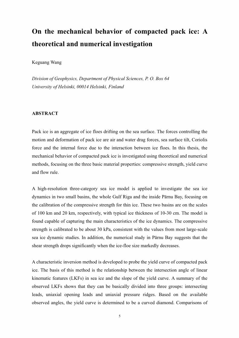
ijkkijij P δεηζεησ ]2)[(2 −−+= && (4)
where σij is the two-dimensional stress tensor, ζ and η are non-linear bulk and shear
viscosities, kkε& is the trace of the two-dimensional strain-rate tensor ijε& , and P is the
pressure in two dimensional mechanics (Hibler, 1979)
)]1(exp[* AChPP −−= , (5)
where P* the compressive strength of ice (dimension force/area), h is the mean ice
thickness and A the ice compactness, and C is the strength reduction constant for lead
opening. The viscosity coefficients ζ and η are functions of the strain-rate invariants and
the ice strength (Hibler, 1979)
∆= 2Pζ , 2eζη = , (6)
where })(,max{ 212220 III e εε && −+∆=∆ , ∆0 is the maximum linear viscous creep rate, e is
the ratio of the compressive strength to shear strength or the aspect ratio of the yield
ellipse, and Iε& and IIε& are the sum and difference of the principal values of ijε& .
Figure 1. The elliptical yield curve and the normal flow rule in the invariant coordinates.
For the isotropic material, the orientations of the principal stresses and principal strain
rates are coincident.
The constitutive law (Eq. 4) and the viscosities (Eq. 6) are a direct outcome of the
elliptical yield curve (Hibler, 1977) and the normal flow rule. A yield curve describes the
limit of any possible combination of stresses. Express the elliptical yield curve in the
invariant form we have
Page 9
9
( ) 022
),(2
22
=
−+
+=
PePF IIIIII σσσσ (7)
where σI and σII are the mean compressive stress and maximum shear stress, respectively.
As can be seen in Figure 1, this elliptical yield curve is centered at (–P/2, 0), with the long
and short axes being P/2 and P/2e, respectively. The normal flow rule states that the
strain-rate vector ( Iε& , IIε& ) is normal to the yield curve at the failure point (Figure 1).
Applying this flow rule, we get
+=
∂∂
=2
2 PFI
II σλ
σλε& (8a)
IIII
II eF σλσ
λε 22=∂∂
=& (8b)
where λ is a nonnegative variable that adjusts its magnitude to prohibit the stress state
from exceeding the yield constraint (Pritchard, 1988; Paper III). It can be determined by
substituting Eqs. (8) into Eq. (7),
PPe III ∆
=+
=− 222 εε
λ&&
(9)
Using the general form of the normal flow rule (e.g. Coon et al., 1974; Paper III), we have
( )ijIijijI
ijijI
IIII
ijij
Iijij
ee
FFF
δσσλδε
σλδε
σσσ
δσ
λσ
λε
−+=+=
∂∂
+∂∂
=∂∂
=
22
2'
2
'2
&&
&
(10)
where ijIijij δσσσ −=' is the stress deviator. From Eqs. (8-10) we get
ijijIij
ijIijIij
ijIijIij
ij
PePP
eP
Pee
δδεε
δλε
λδεε
δσλ
δεεσ
222
2222
22
22
−
∆−
∆+
∆=
−+
−=+
−=
&&
&&&&&
(11)
Denote ∆= 2Pς and ∆= 22ePη , we can easily get the results as shown in Eq. (4).
The above viscous-plastic rheology has so far been the standard constitutive law for
large-scale sea ice dynamics. It is clear that this constitutive law has the mathematical
simplicity and computational facility. However, it has been shown that the elliptical yield
curve is not the physically most appropriate one through model comparisons (e.g. Ip et al.,
1991; Zhang and Rothrock, 2005; Hutchings et al., 2005). There also exist large
Page 10
10
uncertainties in how to formulate the compressive strength, as the different formulations
lead to different dependence on the ice thickness (e.g. Coon, 1974; Rothrock, 1975; Hibler,
1979; Hibler, 1980; Wu and Leppäranta, 1988; Flato and Hibler, 1991; Flato and Hibler,
1995). The flow rule has so far received least attention. The deformation fields (e.g. Kwok,
2001) show that in most cases shear deformation is much larger than divergence and the
present constitutive law is of poor capability to model it (e.g. Geiger et al., 1998).
1.2. Objectives of the Thesis
The overall goal of this thesis is to investigate the mechanical behavior of compacted pack
ice using theoretical and numerical methods, thereby advancing our understanding of the
sea ice dynamics and giving guidance for later modeling studies. Specifically, Papers I and
II investigate the compressive strength of thin pack ice in two small basins using an
existing sea ice dynamic model; Paper III investigates the impact of the constitutive law
on the deformation patterns in pack ice, with special emphasis on the non-normal flow
rules; in Paper IV, a characteristic inversion method is developed, which relates the slope
of the yield curve to the angle between intersecting linear kinematic features (LKFs), to
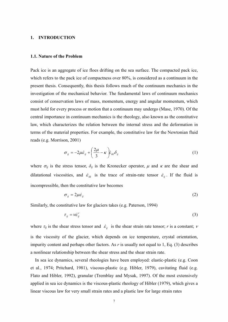
observe the yield curve of compacted pack ice through satellite images.
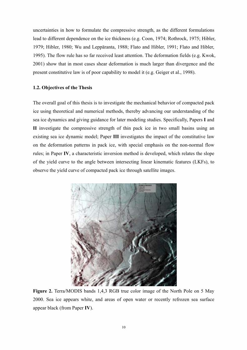
Figure 2. Terra/MODIS bands 1,4,3 RGB true color image of the North Pole on 5 May
2000. Sea ice appears white, and areas of open water or recently refrozen sea surface
appear black (from Paper IV).
Page 11
11
The LKFs in this study refer to the long, narrow geophysical features in pack ice that
are morphologically distinct from the surrounding ice (Paper IV). They may consist of
open water, new ice, young ice, rafted ice, or even ridged ice (Kwok, 2001). A typical
pattern of the LKFs in the central Arctic is shown in Figure 2. In this Terra/MODIS true
color image, sea ice appears white; areas of open water or recently refrozen sea surface
appear black. These dark lines are called leads, being the preferable LKFs for this study.
The intersection angles between these LKFs are normally 20˚ to 60˚, with the most
significant ones being 30˚ to 45˚. The range of these angles is important for determining
the yield curve in Paper IV.
1.3. Main Results Achieved
Papers I and II are a continuation of the early studies of sea ice dynamics in the Baltic Sea
and Bohai Sea (Leppäranta, 1981; Wu and Leppäranta, 1988, 1990; Leppäranta and Zhang,
1992; Zhang and Leppäranta, 1992, 1995; Omstedt et al., 1994; Haapala and Leppäranta,
1996, 1997; Wu et al., 1997; Leppäranta et al., 1998; Zhang, 2000; Leppäranta and Wang,
2002). These two papers focused on the sea ice dynamics in small basins, with particular
emphasis on the calibration of the compressive strength. It is shown that the model works
well in these two small basins and the observed ice dynamic events can be well
reproduced. The compressive strength was calibrated to be about 30 kPa in these two
studies. The shear strength may drop significantly when the ice floes are broken into
blocks of less than 20 m.
Paper IV investigated the relationship between the LKFs and the yield curve. It is found,
through a characteristic analysis of the stress field in the pack ice, that the intersection
angle between LKFs is closely associated with the slope of the yield curve. A summary of
the LKFs shows that they can basically divided into three groups, i.e. intersecting leads,
uniaxial opening leads and uniaxial pressure ridges. Applying the relationship to the
observed LKFs leads to a curved diamond yield curve. This study opened a new
application of satellite remote sensing, and is believed to be able to acquire a realistic
yield curve for pack ice, since the relationship identified here is closely related to the
stress field of the concerned pack ice.
Paper III proposed a new constitutive law by considering the pack ice as a
two-dimensional granular plastic, where the yield curve is the Mohr-Coulomb law with a
limit of maximum principal stress, and the flow rule uses a combination of the normal and
co-axial flow rule. It is shown that this new rheology not only captures the main features
Page 12
12
of forming LKFs but also avoids overestimating divergence during shear deformation.
This study provides an opportunity for selecting the most realistic constitutive law based
on the observations of the strain-rate field.
It is expected that the probed yield curve, flow rule and the compressive strength would
be highly beneficial to modeling applications, in particular the modeling of LKFs-resolved
sea ice patterns. Such applications are, however, out of the present scope and will not be
discussed in detail in the present thesis.
1.4. Author’s Contribution
The author of this thesis is fully responsible for Papers III and IV, and for this summary.
He is mostly responsible for Papers I and II; author’s contributions in these two papers are
both about 2/3.
2. DYNAMIC CALIBRATION OF THE COMPRESSIVE STRENGTH
The compressive strength is one of the key material properties in sea ice dynamics. It has
been shown to be a very sensitive parameter in sea ice numerical modeling (Hibler and
Walsh, 1982; Hibler and Ackley, 1983; Zhang and Leppäranta, 1995; Leppäranta et al.,
1998; Zhang, 2000; Papers I and II). There have been several methods to estimate this
parameter. For example, Coon (1974) considers a buckling mechanism, Rothrock (1975)
and Thorndike et al. (1975) relate it to the potential energy change during ridging. The
method applied here is the dynamic calibration method, which determines the compressive
strength through the comparison of numerical simulations with observations. This method
has long been applied in the sea ice dynamic simulations (e.g. Hibler, 1979; Hibler and
Walsh, 1982; Hibler and Ackley, 1983; Zhang and Leppäranta, 1995; Leppäranta et al.,
1998; Zhang, 2000; Papers I and II).
Sea ice models formulated through ice thickness distribution (ITD) are in principle of
higher capability in estimating the compressive strength, since they provide a more
detailed description of ice conditions than the ice-category-based models. There have been
extensive discussions on the strength and ridging through ITD (e.g. Thorndike et al., 1975;
Rothrock, 1975; Hibler, 1980; Flato and Hibler, 1995; Bitz et al., 2001; Haapala et al.,
2005; Lipscomb et al., 2007). However, most of these studies focus on the comparison of
ITD between the observed and simulated; none has verified the simulated ice velocity
field against the observations. The accuracy in these formulations therefore remains
Page 13
13
uncertain, and these results will not be discussed in the present thesis.
The model used here is the Wu and Leppäranta (1988) model, which follows much of
the Hibler (1979) model with some modifications in the ice categorization and the ice
redistribution scheme. Hibler (1979) separated the ice-covered area into open water and
thick ice, which is traditionally called a two-category model. The present model is a direct
development of his model by further separating the ice into level ice and deformed ice. It
is usually called a three-category ice model among others (e.g. Walsh and Zwally, 1990;
Flato and Hibler, 1991; Harder and Lemke, 1994). A further separation of the deformed ice
into rafted ice and ridged ice is made by Haapala (2000), who also included lead ice in the
level ice.
2.1. Model Description
The basic equations in this model consist of an ice categorization equation, conservation
equations of ice mass and momentum, and a viscous-plastic constitutive law as described
in Section 1.
The ice categorization equation describes the ice conditions,
Ahhm dui )( += ρ , (12)
where m is ice mass, ρi is the ice density, A is the total ice compactness, and AAhh uuu =
and AAhh ddd = are the mean thickness of the level and deformed ice in the
ice-covered region; the actual thickness and compactness of the level and deformed ice, hu,
hd, Au, Ad, are not explicitly utilized in the model. The momentum equation controls the
motion and deformation,
σττuku⋅∇++=
∇+×+ wagf
dtdm ξ , (13)
where dtd is the substantial time derivative, u is the ice velocity, f the Coriolis
parameter, k is the unit upward vector normal to the surface, τa and τw are the air and
water stresses, g is the gravity acceleration, ξ is the sea surface elevation, and σ the
internal ice stress tensor. In order to be consistent with the free-drift limit, the compactness
A is required to be added before the air and water stresses of the momentum equation (e.g.
Connolley et al., 2004; Paper III); however, the difference is very small except where ice
compactness is much lower than unity (Connolley et al., 2004). The air and water stresses
are determined by the bulk formula (McPhee, 1986)
Page 14
14
)sincos( φφρ aaaaaa C UkUUτ ×+= , (14a)
[ ]θθρ sin)(cos)( uUkuUuUτ −×+−−= wwwwww C , (14b)
where ρa and ρw are air and water densities, Ca and Cw are air and water drag coefficients,
Ua and Uw are wind and current velocities, and φ and θ are boundary layer turning angles
for air and water. The mass conservation equation depicts the ice advection and
redistribution,
},,{},,{},,{ duAdudu hhAhhAt
ψψψ∂∂
+∇⋅−= u, (15)
where duA ψψψ ,, are the ice redistribution functions satisfying the following constraint
u⋅∇+−=+++ AhhAhh duduAdu )()()( ψψψ . (16)
The viscous-plastic rheology of Hibler (1979) is applied in the present model with some
modification in the formulation of the pressure,
)]1(exp[* AChPP −−= , (17)
where Ahhh du )( += is the total mean ice thickness (ice volume per unit area), P* is the
compressive strength.
2.2. Model Applications
The numerical model introduced here, as a result of the Chinese-Finnish cooperation in
marine research, has been applied to a variety of purposes. This model was the routine ice
forecast model in the Finnish Ice Service (Bai et al., 1995; Cheng et al., 1999), in the
National Center for Marine Environmental Forecasts of China (Wu and Leppäranta, 1988,
1990; Wu et al., 1998; Wang et al., 1999) and in the Swedish Meteorological and
Hydrological Institute (Omstedt et al., 1994; Omstedt and Nyberg, 1995).
This model has also been intensively used in the investigation of ice dynamics in the
Bohai Sea (e.g. Wu and Leppäranta, 1988, 1990; Wang and Wu, 1994; Wu et al., 1997;
Wang et al., 1999), in the Baltic Sea and its sub-basins (Leppäranta and Zhang, 1992;
Zhang and Leppäranta, 1992, 1995; Leppäranta et al., 1998; Leppäranta and Wang, 2002),
and in large lakes (Wang et al., 2006). The focuses have mainly on the calibration of the
compressive strength and investigation of the scale effect in sea ice dynamics (Leppäranta,
1998, 2005). This model has also been applied to investigate the sea ice dynamics for the
frequency response (Leppäranta and Wang, 2004).
Page 15
15
Coupling of this model with ocean models has been applied to investigate the effect of
sea ice on the sea level variations (Zhang and Leppäranta, 1992, 1995; Omstedt et al.,
1994), and on the seasonal ice climate (Haapala and Leppäranta, 1996, 1997; Zhang et al.,
1997). The interaction between tide and sea ice in Bohai Sea has been studied by Zhang
and Wu (1994), Li (1997) and Su (2001).
The present study (Papers I and II) is a result of the Chinese-Finnish-Estonian
collaboration, initialized by the need of sea ice prediction in the Gulf of Riga and Pärnu
Bay for harbor traffic in Pärnu. Special interest was in the study of sea ice dynamics in
small basins and the investigation of scale effect in the ice thickness and basin size.
2.3. Modeling Results
The modeling study in the present thesis (Papers I and II) is a continuation of the earlier
studies on sea ice dynamics. The main purpose of the modeling was a) to construct a
high-resolution model for routine ice forecast in the Gulf of Riga (Paper I); b) to
investigate the model capability in very small basins and investigate the scale effect
(Papers I and II); c) to calibrate the compressive strength for situations of small basin and
small ice thickness (Papers I and II); d) to study the influence of coastal topography and
islands (Leppäranta and Wang, 2002); and e) to construct a monitoring and forecasting
system for the Gulf of Riga (Kõuts et al., 2006). In this thesis, only the main results of
Papers I and II are summarized.
2.3.1. Tuning of the Rheological Parameters
To validate the model capability running in small basins, the main tuning parameters
would be the rheological parameters and the air and water drag coefficients. In this study,
we employed the air and water drag coefficients obtained in earlier studies (Leppäranta
and Omstedt, 1990). The focus here is therefore on the rheological parameters, including
the compressive strength P* and the ratio of compressive strength to shear strength, e; the
other parameters, e.g. the strength reduction constant for lead opening C and the
maximum linear viscous creep rate ∆0, have all followed the standard values after Hibler
(1979).
Despite the great importance of the compressive strength P* in sea ice dynamics, its
dependence on the ice thickness is, however, not fully understood. Coon (1974) gives a
dependence on the square root of ice thickness, Hibler (1979) gives a constant strength,
and Overland and Pease (1988) propose a linear dependence on the ice thickness. There
Page 16
16
have been a variety of studies to calibrate the ice compressive strength for thick ice and in
large basins (e.g. Hibler and Walsh, 1982; Hibler and Ackley, 1983; Flato and Hibler, 1991;
Leppäranta et al., 1998; Zhang, 2000). The present study is therefore significant to provide
the results for thin ice and small basins, because the formulation of the compressive
strength must be appropriate for both thin ice and thick ice. To the author’s knowledge,
there have been no such studies before.
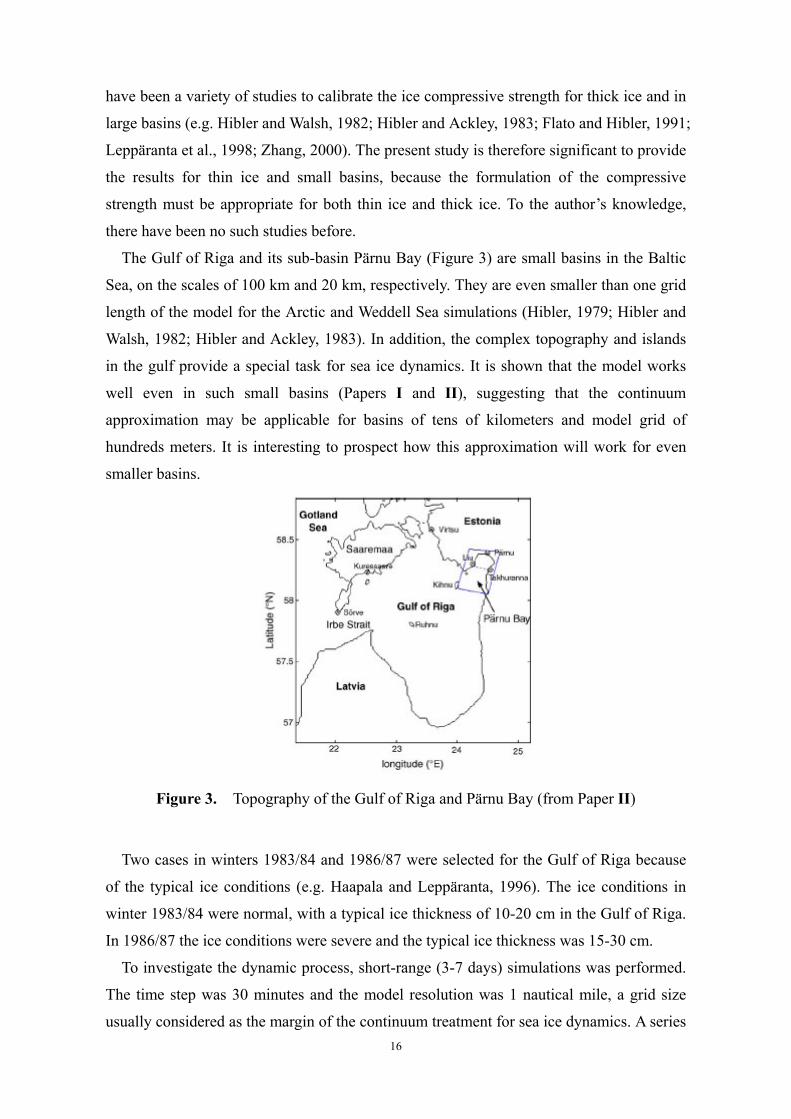
The Gulf of Riga and its sub-basin Pärnu Bay (Figure 3) are small basins in the Baltic
Sea, on the scales of 100 km and 20 km, respectively. They are even smaller than one grid
length of the model for the Arctic and Weddell Sea simulations (Hibler, 1979; Hibler and
Walsh, 1982; Hibler and Ackley, 1983). In addition, the complex topography and islands
in the gulf provide a special task for sea ice dynamics. It is shown that the model works
well even in such small basins (Papers I and II), suggesting that the continuum
approximation may be applicable for basins of tens of kilometers and model grid of
hundreds meters. It is interesting to prospect how this approximation will work for even
smaller basins.
Figure 3. Topography of the Gulf of Riga and Pärnu Bay (from Paper II)
Two cases in winters 1983/84 and 1986/87 were selected for the Gulf of Riga because
of the typical ice conditions (e.g. Haapala and Leppäranta, 1996). The ice conditions in
winter 1983/84 were normal, with a typical ice thickness of 10-20 cm in the Gulf of Riga.
In 1986/87 the ice conditions were severe and the typical ice thickness was 15-30 cm.
To investigate the dynamic process, short-range (3-7 days) simulations was performed.
The time step was 30 minutes and the model resolution was 1 nautical mile, a grid size
usually considered as the margin of the continuum treatment for sea ice dynamics. A series
Page 17
17
of sensitivity experiments was performed to determine an optimal compressive strength
for the Gulf of Riga. The compressive strength P* was set to be 10, 30 and 50 kPa,
respectively. The air and water drag coefficients and the turn angles, being 0.0018, 0.0035
and 17˚, were obtained from Leppäranta and Omstedt (1990), being a set of standard
parameters for all the ice dynamic studies in the Baltic Sea. The other rheological
parameters (e, C, and ∆0) were all taken from standard values (Hibler, 1979). The
numerical studies in Paper I show that the model is capable of reproducing the main
characteristics of ice drift and deformation processes in the Gulf of Riga. It is also shown
that the optimized compressive strength is 30 kPa.
Paper II is a continuation of ice dynamic study of Paper I toward an even smaller basin.
The select dynamic ice event took place in 1-15 February 2002 in Pärnu Bay, with a
typical ice thickness of 10-30 cm. The ice was in most time immobile except on 4-5 the
ice floes were broken into small blocks by a strong storm and on 13-14 February half of
the ice cover flowed out of Pärnu Bay. Such situations are getting more and more common
in recent years.
Three 5-day simulations were performed to investigate the ice dynamic events. The
model grid here was down to 463 m and time step to 5 minutes. Similar sensitive
experiments were performed to calibrate the compressive strength and to simulate the
deformation history of the ice cover. The compressive strength was again found to be
about 30 kPa.
To interpret the ice cover remaining immobile under higher wind but flew out of Pärnu
Bay, it is found that a larger aspect ratio of the yield ellipse, e = 10, is necessary (Paper II).
This is explained by the fact that the ice floes were broken into small blocks during the
strong storm process. However, since this is only one case study, more verification would
be favorable.
2.3.2. Scale Analysis
Ice forms in the Gulf of Riga annually, and the length of the ice season is 3-5 months. In
mild winters ice only covers the northern part, mainly in the Pärnu Bay, while in normal or
severe winters the whole basin freezes over. The thickness of undeformed drift ice is
typically 10-30 cm. The ice cover in the whole gulf is usually mobile; but in Pärnu Bay the
ice thickness is usually large enough to form stable fast ice, except in mild winters thin
fast ice may be broken by strong winds. These facts suggest that the ice in the Gulf of
Riga and Pärnu Bay is in the demarcation between stable and unstable conditions.
Page 18
18
The basis of the scale analysis is the ice momentum balance. It is can be considered as a
simplified form of the dynamic calibration method. To break the ice cover, the condition
for unstable ice cover must be satisfied (Leppäranta, 1998, 2005; Paper II)
HPLa*>τ , (18)
where L is the fetch of wind over the ice-covered area, H is the typical ice thickness.
Take typical scales in the Gulf of Riga: L = 100 km, H = 30 cm, Ua = 10 m/s; and
consider that the ice is commonly mobile (Paper I), we get P* < 78 kPa according to Eq.
(18). Referring to the wind and ice conditions during 1-15 February 2002 in Pärnu Bay
(Paper II), we have typical scales L = 20 km, H = 30 cm, Ua = 10 m/s for the stable ice
cover, from which we get P* ≥ 15.6 kPa. Similarly, we have typical scales L = 20 km, H =
30 cm, Ua = 20 m/s for the unstable ice cover (Paper II), we have P* < 62.4 kPa. Therefore,
a reasonable estimate for the ice thickness of 30 cm is between 15.6 kPa and 62.4 kPa.
Take typical scales L = 20 km, H = 10 cm, Ua = 8 m/s for the stable pack ice in Pärnu
Bay (Paper II), we have an estimate of the compressive strength for ice thickness of 10 cm
P* ≥ 30 kPa. Because the compressive strength of thicker ice is usually larger than that of
thinner ice, it is reasonable to conclude that the compressive strength for ice thickness of
10 – 30 cm is in the range of 30 – 60 kPa.
A more comprehensive scale analysis can be made by taking into account the yield
curve and considering the orientations of the wind and coast (e.g. Pritchard, 1976;
Tremblay and Hakakian, 2006). Using the elliptical yield curve and taking the elliptical
aspect ratio e = 2 results in a minor change in the result (Tremblay and Hakakian, 2006),
with about 10% difference. As the wind velocity is almost perpendicular to the coast in the
present study, the estimated compressive strength is believed to be comparable to their
results.
2.4. Comparison with the Other Studies
The ice compressive strength calibrated from Papers I and II is most probably close to 30
kPa for the ice thickness typical of 10 – 30 cm. This value is consistent with the results
calibrated from most of the other regions with mean ice thickness ranging from about 3.0
m in the Arctic (e.g. Hibler and Walsh, 1982; Flato and Hibler, 1991), through about 0.8 m
in the Weddell Sea (e.g. Hibler and Ackley, 1983; Geiger et al., 1998), to about 0.5 m in
the Bothnian Bay (e.g. Haapala and Leppäranta, 1996; Zhang, 2000).
Page 19
19
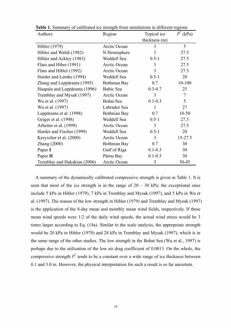
Table 1. Summary of calibrated ice strength from simulations in different regions Authors Region Typical ice
thickness (m) P* (kPa)
Hibler (1979) Arctic Ocean 3 5 Hibler and Walsh (1982) N Hemisphere 3 27.5 Hibler and Ackley (1983) Weddell Sea 0.5-1 27.5 Flato and Hiber (1991) Arctic Ocean 3 27.5 Flato and Hibler (1992) Arctic Ocean 3 27.5 Harder and Lemke (1994) Weddell Sea 0.5-1 20 Zhang and Leppäranta (1995) Bothnian Bay 0.7 10-100 Haapala and Leppäranta (1996) Baltic Sea 0.3-0.7 25 Tremblay and Mysak (1997) Arctic Ocean 3 7 Wu et al. (1997) Bohai Sea 0.1-0.3 5 Wu et al. (1997) Labrador Sea 1 27 Leppäranta et al. (1998) Bothnian Bay 0.7 10-50 Geiger et al. (1998) Weddell Sea 0.5-1 27.5 Arbetter et al. (1999) Arctic Ocean 3 27.5 Harder and Fischer (1999) Weddell Sea 0.5-1 20 Kreyscher et al. (2000) Arctic Ocean 3 15-27.5 Zhang (2000) Bothnian Bay 0.7 30 Paper I Gulf of Riga 0.1-0.3 30 Paper II Pärnu Bay 0.1-0.3 30 Tremblay and Hakakian (2006) Arctic Ocean 3 30-45
A summary of the dynamically calibrated compressive strength is given in Table 1. It is
seen that most of the ice strength is in the range of 20 – 30 kPa; the exceptional ones
include 5 kPa in Hibler (1979), 7 kPa in Tremblay and Mysak (1997), and 5 kPa in Wu et
al. (1997). The reason of the low strength in Hibler (1979) and Tremblay and Mysak (1997)
is the application of the 8-day mean and monthly mean wind fields, respectively. If these
mean wind speeds were 1/2 of the daily wind speeds, the actual wind stress would be 3
times larger according to Eq. (14a). Similar to the scale analysis, the appropriate strength
would be 20 kPa in Hibler (1979) and 28 kPa in Tremblay and Mysak (1997), which is in
the same range of the other studies. The low strength in the Bohai Sea (Wu et al., 1997) is
perhaps due to the utilization of the low air drag coefficient of 0.0013. On the whole, the
compressive strength P* tends to be a constant over a wide range of ice thickness between
0.1 and 3.0 m. However, the physical interpretation for such a result is so far uncertain.
Page 20
20
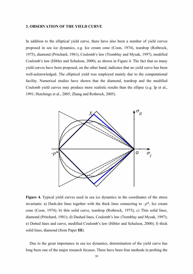
3. OBSERVATION OF THE YIELD CURVE
In addition to the elliptical yield curve, there have also been a number of yield curves
proposed in sea ice dynamics, e.g. Ice cream cone (Coon, 1974), teardrop (Rothrock,
1975), diamond (Pritchard, 1981), Coulomb’s law (Tremblay and Mysak, 1997), modified
Coulomb’s law (Hibler and Schulson, 2000), as shown in Figure 4. The fact that so many
yield curves have been proposed, on the other hand, indicates that no yield curve has been
well-acknowledged. The elliptical yield was employed mainly due to the computational
facility. Numerical studies have shown that the diamond, teardrop and the modified
Coulomb yield curves may produce more realistic results than the ellipse (e.g. Ip et al.,
1991; Hutchings et al., 2005; Zhang and Rothrock, 2005).
σI
σIIX
-p* o
Figure 4. Typical yield curves used in sea ice dynamics in the coordinates of the stress
invariants: a) Dash-dot lines together with the thick lines connecting to –p*, Ice cream
cone (Coon, 1974); b) thin solid curve, teardrop (Rothrock, 1975); c) Thin solid lines,
diamond (Pritchard, 1981); d) Dashed lines, Coulomb’s law (Tremblay and Mysak, 1997);
e) Dotted lines and curve, modified Coulomb’s law (Hibler and Schulson, 2000); f) thick
solid lines, diamond (from Paper III).
Due to the great importance in sea ice dynamics, determination of the yield curve has
long been one of the major research focuses. There have been four methods in probing the
Page 21
21
yield curve, namely energy estimation (e.g. Thorndike et al, 1975; Rothrock, 1975; Ukita
and Moritz, 1995, 2000), dynamic comparison (Ip et al., 1991; Geiger et al., 1998;
Hutchings et al., 2005; Zhang and Rothrock, 2005), particle simulation (Hopkins and
Hibler, 1991a; Hopkins, 1994, 1996, 1998, 2001), and scale-independent extending
(Schulson and Hibler, 1991; Hibler and Schulson, 2000; Schulson, 2001, 2004). However,
the main problem in these methods is the indirect derivation; none is based on the stress
field of the real concerned pack ice. It is the purpose of Paper IV to develop a
stress-associated method to observe the yield curve.
3.1. The Characteristic Inversion Method
The method developed here uses the characteristic analysis, assuming an isotropic ice
cover, a quasi-steady deformation, a full coverage of the observed intersection angles and
the corresponding slopes, and a convex postulate for the yield curve. The basis for
observing the yield curve is the relationship between the angle between intersecting LKFs
and the slope of the yield curve (see details in Paper IV)
)2arctan(cos θβ = or )arccos(tan2 βθ = . (19)
where β is the slope of the yield curve, and 2θ is the angle between intersecting LKFs.
This relationship shows that the slope of the yield curve is only dependent on the
intersection angle between LKFs and vice versa. Their relationship is shown in Figure 5,
where 2θ takes real values only when β ranges from -45˚ to 45˚. As can be seen, 2θ ranges
from 90˚ to 180˚ when β is negative, while it changes within 0˚ and 90˚ when β is positive.
In addition, when 2θ changes from 0˚ to 60˚ or from 120˚ to 180˚, β varies quite slowly;
while for the remaining situations, β changes rather rapidly.
It should be noted that the intersection angle 2θ must contain the major principal
direction (MPD) as the bisector. As defined, the MPD is the line along the larger algebraic
principal stress (Paper IV). Therefore, when ice cover undergoes uniaxial compression,
the LKFs (pressure ridges) are along the MPD, resulting in 2θ being equal to 0˚. On the
other hand, when ice cover undergoes uniaxial tension, the LKFs (uniaxial opening leads)
are perpendicular to the MPD, resulting in 2θ being equal to 180˚. For other situations, the
determination of the MPD may rely on a detailed calculation.
Page 22
22
0 15 30 45 60 75 90 105 120 135 150 165 180-45
-30
-15
0
15
30
45
β ( °
)
2θ (°) Figure 5. Relationship between the slope of the yield curve, β, and the angle between
LKFs, 2θ (from Paper IV).
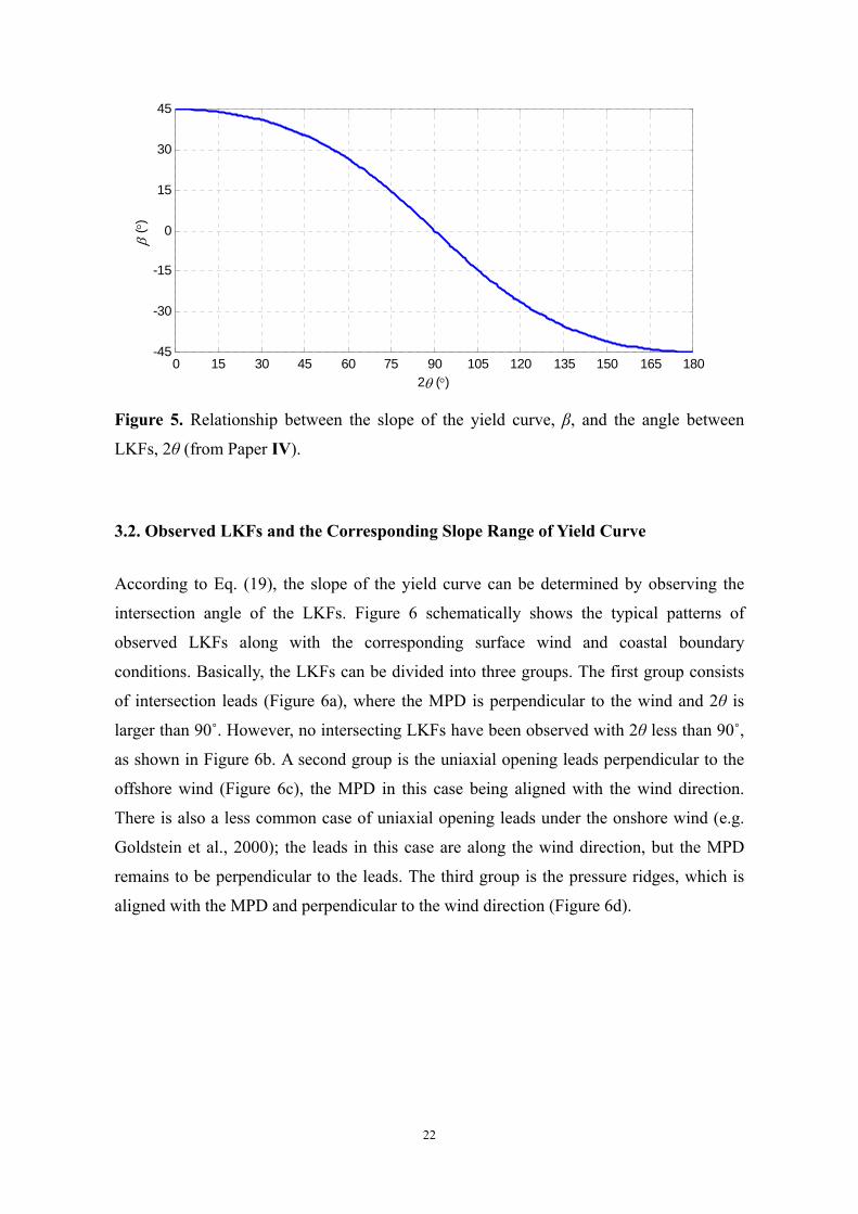
3.2. Observed LKFs and the Corresponding Slope Range of Yield Curve
According to Eq. (19), the slope of the yield curve can be determined by observing the
intersection angle of the LKFs. Figure 6 schematically shows the typical patterns of
observed LKFs along with the corresponding surface wind and coastal boundary
conditions. Basically, the LKFs can be divided into three groups. The first group consists
of intersection leads (Figure 6a), where the MPD is perpendicular to the wind and 2θ is
larger than 90˚. However, no intersecting LKFs have been observed with 2θ less than 90˚,
as shown in Figure 6b. A second group is the uniaxial opening leads perpendicular to the
offshore wind (Figure 6c), the MPD in this case being aligned with the wind direction.
There is also a less common case of uniaxial opening leads under the onshore wind (e.g.
Goldstein et al., 2000); the leads in this case are along the wind direction, but the MPD
remains to be perpendicular to the leads. The third group is the pressure ridges, which is
aligned with the MPD and perpendicular to the wind direction (Figure 6d).
Page 23
23
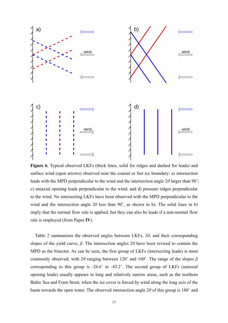
a)
wind
b)
wind
d)
wind
c)
wind
Figure 6. Typical observed LKFs (thick lines, solid for ridges and dashed for leads) and
surface wind (open arrows) observed near the coastal or fast ice boundary: a) intersection
leads with the MPD perpendicular to the wind and the intersection angle 2θ larger than 90˚;
c) uniaxial opening leads perpendicular to the wind; and d) pressure ridges perpendicular
to the wind. No intersecting LKFs have been observed with the MPD perpendicular to the
wind and the intersection angle 2θ less than 90˚, as shown in b). The solid lines in b)
imply that the normal flow rule is applied, but they can also be leads if a non-normal flow
rule is employed (from Paper IV).
Table 2 summarizes the observed angles between LKFs, 2θ, and their corresponding
slopes of the yield curve, β. The intersection angles 2θ have been revised to contain the
MPD as the bisector. As can be seen, the first group of LKFs (intersecting leads) is most
commonly observed, with 2θ ranging between 120˚ and 160˚. The range of the slopes β
corresponding to this group is -26.6˚ to -43.2˚. The second group of LKFs (uniaxial
opening leads) usually appears in long and relatively narrow areas, such as the northern
Baltic Sea and Fram Strait, when the ice cover is forced by wind along the long axis of the
basin towards the open water. The observed intersection angle 2θ of this group is 180˚ and
Page 24
24
the corresponding slope β is -45˚. The third group of LKFs (pressure ridges) is created by
uniaxial compression. The intersection angle 2θ of this group is 0° and the corresponding
slope β is 45˚.
Table 2. Observed angles between intersecting LKFs, 2θ, and the corresponding slope of the yield curve, β (from Paper IV) Authors Sea area 2θ (˚) β (˚) Marko and Thomson (1977) Canada Basin 140–160 -37.5– -43.2 Leppäranta (1983b) Baltic Sea 146–154 -39.7– -41.9 Vinje and Finnekåsa (1986) Fram Strait 147–153 -40.0– -41.7 Fily and Rothrock (1986) central Arctic 146–158 -39.7– -42.8 Erlingsson (1988) Greenland Coast 145–151 -39.2– -41.2 Pritchard (1992) Fram Strait 90, 120, 180 0, -26.6, -45 Walter and Overland (1993) Beaufort Sea 130–160, 180 -32.7– -43.2, -45 Cunningham et al. (1994) Beaufort Sea 140–150 -37.5– -40.9 Overland et al. (1995) Arctic Ocean 140–160, 180 -37.5– -43.2, -45 Leppäranta et al. (1998) Baltic Sea 180 -45 Overland et al. (1998) Arctic Ocean 130–160, 180 -32.7– -43.2, -45 Goldstein et al. (2000) Baltic Sea 0, 180 45, -45 Schulson (2004) Arctic Ocean 120–150 -26.6– -40.9 Wang (2004) central Arctic 120–160 -26.6– -43.2
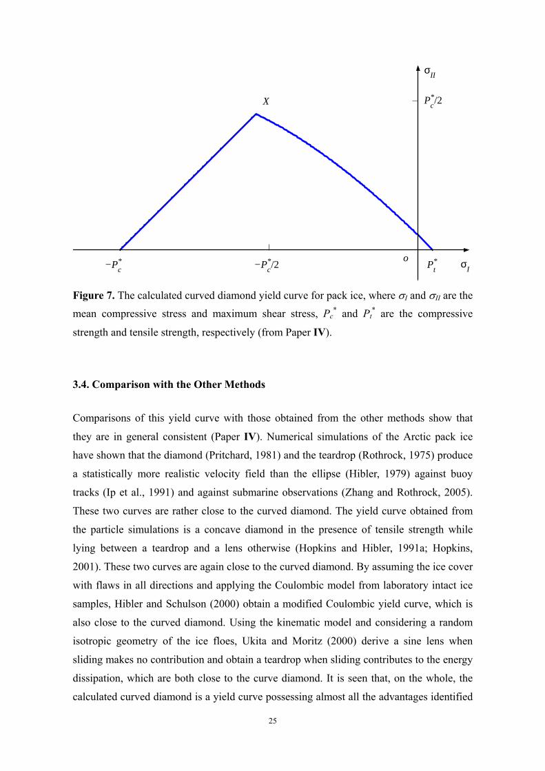
3.3. The Observed Yield Curve
According to the relationship between 2θ and β (Eq. 19), the resulting yield curve is a
curved diamond, as described by the following equations (Paper IV),
IXIcIcII PifP σσσσ ≤≤−+= ** , , (20a)
0,)1)(( 21** <<+−= IIXcIItII ifPP σσασσµσ (20b)
** 0, tIItII PifP ≤≤−= σσσ , (20c)
where σIX is the mean compressive stress at the intersection point X (see Figure 7), and Pt*
= Pc*/20, µ = 1, α = 0.75, and σIX = -0.542Pc
*.
Page 25
25
−P*c
−P*c/2
oP*
tσ
I
P*c/2
σII
X
Figure 7. The calculated curved diamond yield curve for pack ice, where σI and σII are the
mean compressive stress and maximum shear stress, Pc* and Pt
* are the compressive
strength and tensile strength, respectively (from Paper IV).
3.4. Comparison with the Other Methods
Comparisons of this yield curve with those obtained from the other methods show that
they are in general consistent (Paper IV). Numerical simulations of the Arctic pack ice
have shown that the diamond (Pritchard, 1981) and the teardrop (Rothrock, 1975) produce
a statistically more realistic velocity field than the ellipse (Hibler, 1979) against buoy
tracks (Ip et al., 1991) and against submarine observations (Zhang and Rothrock, 2005).
These two curves are rather close to the curved diamond. The yield curve obtained from
the particle simulations is a concave diamond in the presence of tensile strength while
lying between a teardrop and a lens otherwise (Hopkins and Hibler, 1991a; Hopkins,
2001). These two curves are again close to the curved diamond. By assuming the ice cover
with flaws in all directions and applying the Coulombic model from laboratory intact ice
samples, Hibler and Schulson (2000) obtain a modified Coulombic yield curve, which is
also close to the curved diamond. Using the kinematic model and considering a random
isotropic geometry of the ice floes, Ukita and Moritz (2000) derive a sine lens when
sliding makes no contribution and obtain a teardrop when sliding contributes to the energy
dissipation, which are both close to the curve diamond. It is seen that, on the whole, the
calculated curved diamond is a yield curve possessing almost all the advantages identified
Page 26
26
by the other methods.
Unlike the other methods using indirect deductions, the present yield curve is
constructed on observations directly associated with the stress field in the pack ice. As
more and more observations become available, this method is very likely to be a valid
candidate to determine a realistic yield curve for sea ice. Furthermore, it also greatly
facilitates the observations, since measuring angles is much easier than tracking the
deformation field or tracking the production of open water or ice ridges.
From the curved diamond yield curve we can see that the failure stress during shear is
in most time on a state close to the uniaxial compression. This situation is consistent with
the recent field observations of stress tensors in ice floes (Coon et al., 1998; Richter-
Menge and Elder, 1998; Richter-Menge et al., 2002).
4. A COMBINED NORMAL AND NON-NORMAL FLOW RULE
The research on the flow rule of pack ice has been very rare. Early studies generally
postulate that the normal flow rule is followed in sea ice dynamics (e.g. Coon, 1974; Coon
et al., 1974; Rothrock, 1975; Hibler, 1979; Pritchard, 1981). This is natural as the flow
rule cannot be verified before the determination of the yield curve. Ukita and Moritz
(1995), applying the kinematic model and the idea of minimization of the maximum shear
stress, tried to prove the validity of normality; however, their proof is obscured due to the
presumption of a constant ratio of ridging to sliding on the whole band of the deformation
rate. The proof of such a constant ratio is not easier than the normality itself.
4.1. The Co-Axial Flow Rule
The application of the normal flow rule with the elliptical yield curve is shown in Section
1. In Paper III we introduced a new flow rule, the so-called co-axial flow rule for sea ice
dynamics. This flow rule has commonly been applied in the mechanics of granular
material (e.g. Nedderman, 1992). This flow rule states that the strain-rate and stress
deviators are proportional,
ijij ''' σλε =& (21)
where λ' is a scalar variable. This condition leads to the principal stresses and the principal
rates of strain being co-axial. The normal flow rule is a special case of the co-axial flow
rule (Paper III).
Page 27
27
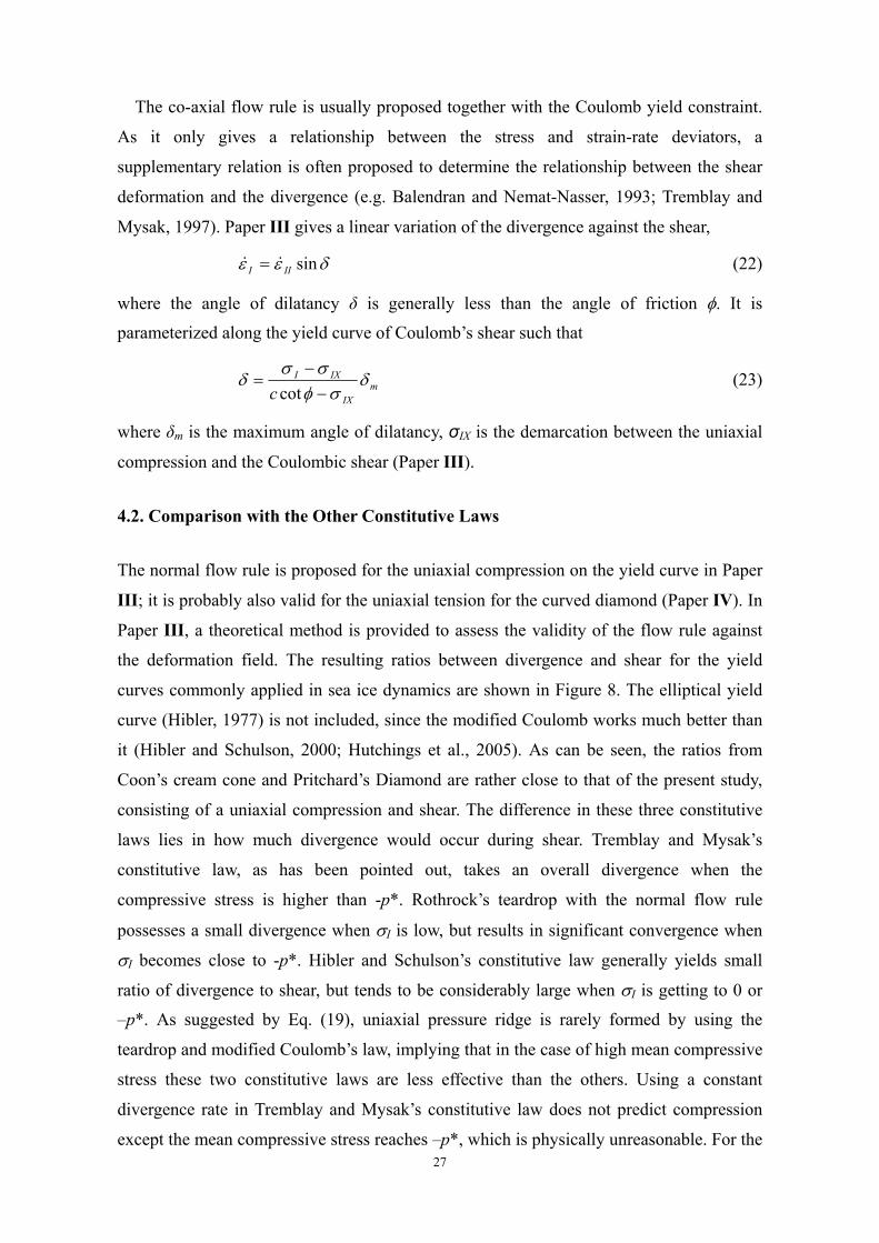
The co-axial flow rule is usually proposed together with the Coulomb yield constraint.
As it only gives a relationship between the stress and strain-rate deviators, a
supplementary relation is often proposed to determine the relationship between the shear
deformation and the divergence (e.g. Balendran and Nemat-Nasser, 1993; Tremblay and
Mysak, 1997). Paper III gives a linear variation of the divergence against the shear,
δεε sinIII && = (22)
where the angle of dilatancy δ is generally less than the angle of friction φ. It is
parameterized along the yield curve of Coulomb’s shear such that
mIX
IXI
cδ
σφσσ
δ−
−=
cot (23)
where δm is the maximum angle of dilatancy, σIX is the demarcation between the uniaxial
compression and the Coulombic shear (Paper III).
4.2. Comparison with the Other Constitutive Laws
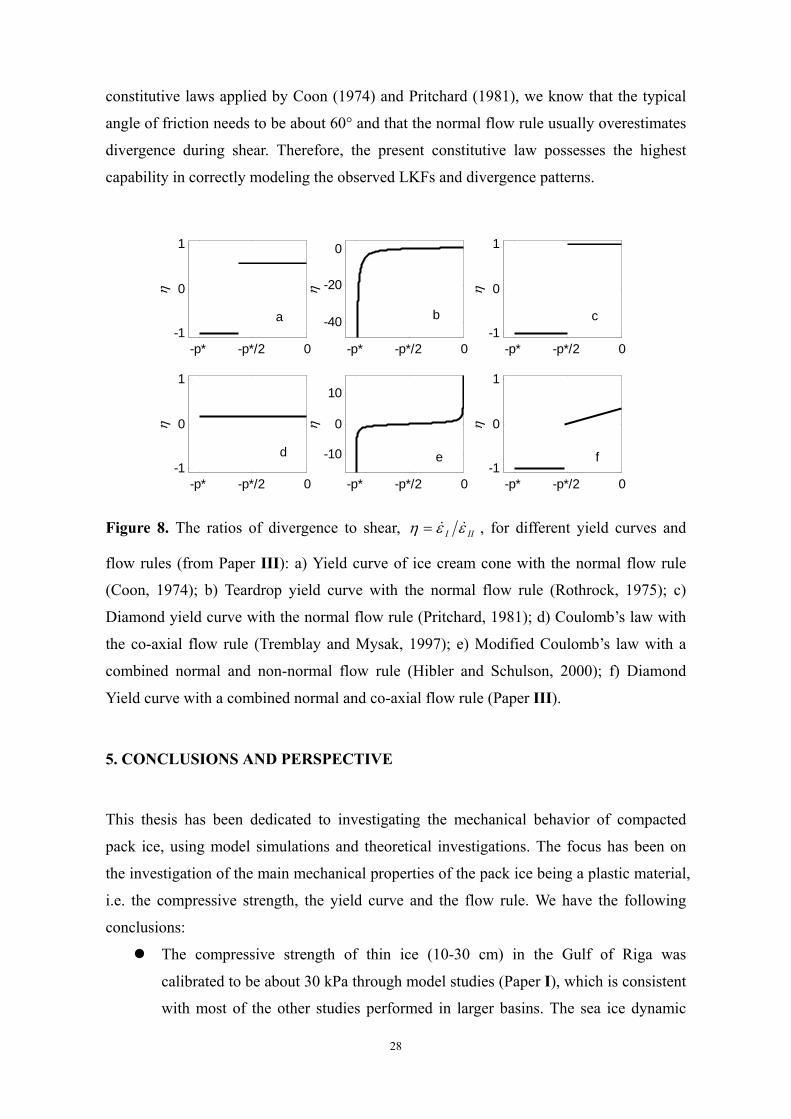
The normal flow rule is proposed for the uniaxial compression on the yield curve in Paper
III; it is probably also valid for the uniaxial tension for the curved diamond (Paper IV). In
Paper III, a theoretical method is provided to assess the validity of the flow rule against
the deformation field. The resulting ratios between divergence and shear for the yield
curves commonly applied in sea ice dynamics are shown in Figure 8. The elliptical yield
curve (Hibler, 1977) is not included, since the modified Coulomb works much better than
it (Hibler and Schulson, 2000; Hutchings et al., 2005). As can be seen, the ratios from
Coon’s cream cone and Pritchard’s Diamond are rather close to that of the present study,
consisting of a uniaxial compression and shear. The difference in these three constitutive
laws lies in how much divergence would occur during shear. Tremblay and Mysak’s
constitutive law, as has been pointed out, takes an overall divergence when the
compressive stress is higher than -p*. Rothrock’s teardrop with the normal flow rule
possesses a small divergence when σI is low, but results in significant convergence when
σI becomes close to -p*. Hibler and Schulson’s constitutive law generally yields small
ratio of divergence to shear, but tends to be considerably large when σI is getting to 0 or
–p*. As suggested by Eq. (19), uniaxial pressure ridge is rarely formed by using the
teardrop and modified Coulomb’s law, implying that in the case of high mean compressive
stress these two constitutive laws are less effective than the others. Using a constant
divergence rate in Tremblay and Mysak’s constitutive law does not predict compression
except the mean compressive stress reaches –p*, which is physically unreasonable. For the
Page 28
28
constitutive laws applied by Coon (1974) and Pritchard (1981), we know that the typical
angle of friction needs to be about 60° and that the normal flow rule usually overestimates
divergence during shear. Therefore, the present constitutive law possesses the highest
capability in correctly modeling the observed LKFs and divergence patterns.
-p* -p*/2 0-1
0
1
η
-p* -p*/2 0
-40
-20
0
η
-p* -p*/2 0-1
0
1
η-p* -p*/2 0
-1
0
1
η
-p* -p*/2 0
-10
0
10
η
-p* -p*/2 0-1
0
1
η
a b c
d e f
Figure 8. The ratios of divergence to shear, III εεη &&= , for different yield curves and
flow rules (from Paper III): a) Yield curve of ice cream cone with the normal flow rule
(Coon, 1974); b) Teardrop yield curve with the normal flow rule (Rothrock, 1975); c)
Diamond yield curve with the normal flow rule (Pritchard, 1981); d) Coulomb’s law with
the co-axial flow rule (Tremblay and Mysak, 1997); e) Modified Coulomb’s law with a
combined normal and non-normal flow rule (Hibler and Schulson, 2000); f) Diamond
Yield curve with a combined normal and co-axial flow rule (Paper III).
5. CONCLUSIONS AND PERSPECTIVE
This thesis has been dedicated to investigating the mechanical behavior of compacted
pack ice, using model simulations and theoretical investigations. The focus has been on
the investigation of the main mechanical properties of the pack ice being a plastic material,
i.e. the compressive strength, the yield curve and the flow rule. We have the following
conclusions:
The compressive strength of thin ice (10-30 cm) in the Gulf of Riga was
calibrated to be about 30 kPa through model studies (Paper I), which is consistent
with most of the other studies performed in larger basins. The sea ice dynamic
Page 29
29
model applied is based on the conservation laws of ice mass and momentum
together with a three-category ice state (open water, undeformed ice and
deformed ice) and a viscous-plastic rheology. The grid size was 1 nautical mile
and time step was 30 minutes. It is shown that the main characteristics of the sea
ice dynamics in the Gulf of Riga can be well reproduced.
The compressive strength of the thin fast ice sheet (about 30 cm) was estimated to
be between 30 and 60 kPa through scale analysis; and the compressive strength of
the thin pack ice (about 10 cm) was calibrated to be again about 30 kPa in Pärnu
Bay, a small basin of 15 km across in the Gulf of Riga (Paper II). The same sea
ice dynamics model was used except that the grid size was down to 1/4 nautical
mile and time step to 5 minutes. The model successfully reproduced the stable ice
situations during 1-5 and 6-12 February 2002 and the severe deformation process
during 5-6 February 2002.
In order to correctly capture the phenomena that the ice cover remained immobile
in high wind but flew out of Pärnu Bay under a mild wind during 13-14 February
2002 (Paper II), It is found, through a series of sensitivity experiments, that the
shear strength needs to drop significantly. The reason for such a change has been
owing to the breakage of the ice floes into small blocks of less than 20 m across.
It is expected that similar effect would also exert in the summer polar oceans and
in seas full of small ice floes.
A method for observing the yield curve of compacted pack ice is developed based
on the characteristic analysis (Paper IV). The analysis shows that the slope of the
yield curve is only dependent on the angle between intersecting LKFs. The basic
assumption made in this analysis is the isotropy, which is generally satisfied in
the homogeneous ice cover.
Using the characteristic inversion method and available observations of the LKFs,
it is found that the yield curve of compacted pack is a curved diamond (Paper IV).
The observed LKFs can basically be divided into 3 groups: intersecting leads,
uniaxial opening leads and uniaxial pressure ridges. The first group of LKFs
(intersecting leads) is most commonly observed, with the intersection angle 2θ
ranging between 120˚ and 160˚ and the corresponding slopes β -26.6˚ to -43.2˚.
The intersection angle of the second group of LKFs (uniaxial opening leads) is
180˚ and the corresponding slope β is -45˚. The intersection angle 2θ of the third
group of LKFs (pressure ridges) is 0° and the corresponding slope β is 45˚.
The new constitutive law proposed in Paper III consists of Coulomb’s friction
Page 30
30
law describing the in-plane shear and the maximum principal stress law
describing the out-of-plane uniaxial compression. For the shear deformation, the
co-axial flow rule with a dilatancy linearly dependent on the shear is proposed;
while for the uniaxial compression, the normal flow rule is shown to be
appropriate. This constitutive law is not only capable to simulate the in-plane
shear and out-of-plane uniaxial compression, but also capable to avoid
overestimating divergence during shear.
Based on the studies performed and the results obtained, it is noteworthy to continue the
following studies in the future:
The result that thin ice of thickness 10-30 cm still has a P* of about 30 kPa
suggests that the compressive strength tends to be a constant over a wide range of
ice thickness. A physically consistent explanation of this result would therefore be
necessary. It is expected that such an explanation will help reveal the material
properties of the compacted pack ice.
Determination of the flow rule from observations would greatly improve our
understanding in sea ice dynamics and our capability in modeling the sea ice
dynamics. A feasible method is provided in Paper III to estimate the flow rule,
which is worthy for a thorough study.
Of the most significant of the present study is that it provides a basis for the
formulation of the next-generation sea ice dynamic model, which characterizes
with high-resolution LKFs-resolved features. This work is currently underway.
Page 31
31
ACKNOWLEDGEMENTS
This study was performed in the Division of Geophysics, Department of Physical Sciences, University
of Helsinki. I would especially like to thank those people and groups who made this thesis possible.
I would like to express my greatest gratitude to Professor Matti Leppäranta, my supervisor, for
providing me continuous support and excellent working conditions in Finland over these years. I
enjoyed the inspiring discussions with him in the Finnish sauna in the white winter and in the bright
summer in his beautiful garden. His enthusiasm, guidance, help and encouragement have greatly
sustained me since the beginning of my study in 2001. Cooperation with Dr. Tarmo Kõuts has been
very helpful to this thesis. I would also like to express my thanks to his hospitality during many visits
to Estonia.
I am deeply indebted to my master supervisors Professor Wu Huiding and Professor Liu Baozhang
for their persistent support and encouragement to my research since 1994. In particular, I would like to
thank Professor Wu for guiding me into this amazingly interesting sea ice studies in 1995. Also, Dr.
Zhang Zhanhai is gratefully thanked for introducing me to Finland and the many helps later on.
Grateful thanks are due to Professor Aike Beckman for his many valuable lectures and discussions,
which enriched much of my perspective over marine science. I would also like to thank Professor Lauri
Pesonen, for his kindly help during the year when Matti was in his sabbatical leave.
I wish to express my sincere thanks to Dr. Jari Haapala and Professor Jüri Elken for their critical
comments and criticism on the manuscript. I am also grateful to Jari for the helpful discussions on sea
ice modeling over the years at Kumpula Campus and in the Finnish Institute of Marine Research.
Dr. Cheng Bin has helped me greatly in my study and life through these years. I will always warmly
remember our time in Helsinki.
The European Commission is kindly acknowledged for the funds through the projects of ‘CLIME’,
‘IRIS’ and ‘SAFEICE’. This work was also supported by the Centre for International Mobility of
Finland, Maj and Tor Nessling Foundation of Finland and Kone Foundation of Finland.
Finally, I am indebted to my parents for their continuous encouragement, to my wife Caixin for her
understanding and continuous support during the years of this work, and to my lovely daughter Xi for
giving me persistent happiness after work from office.
Page 32
32
REFERENCES
Bai, S., H. Grönvall and A. Seinä (1995), The numerical sea ice forcast in Finland in the winter
1993-1994, Report Series of Finnish Institute of Marine Research, MERI 21, 4-11.
Bitz, C. M., M. M. Holland, A. J. Weaver and M. Eby (2001), Simulating the ice thickness distribution
in a coupled climate model, J. Geophys. Res., 106, 2441-2463.
Cheng, B. A. Seinä, J. Vainio, S. Kalliosaari, H. Grönvall and J. Launiainen (1999), Numerical sea ice
forecast in the Finnish Ice Service, Proc. 15th POAC, Espoo, Finland, pp. 131-140.
Connolley, W.M., J.M. Gregory, E. Hunke and A.J. Mclaren (2004), On the consistent scaling of terms
in the sea-ice dynamics Eq., J. Phys. Oceangr., 34, 1776-1780.
Coon, M. D. (1974), Mechanical behavior of compacted Arctic ice floes, J. Petrol. Tech., 26, 466-470.
Coon, M. D., G. A. Maykut, R. S. Pritchard, D. A. Rothrock, and A. S. Thorndike (1974), Modeling the
pack ice as an elastic-plastic material, AIDJEX Bull. 24, pp. 1-106, Univ. of Wash., Seattle, Wash.
Cunningham G. F., R. Kwok and J. Banfield (1994), Ice lead orientation characteristics in the winter
Beaufort Sea, in Proceedings of IGARSS, 1747-1749, Pasadena, CA.
Erlingsson, B. (1988), Two-dimensional deformation patterns in sea ice, J. Glaciol., 34, 301-308.
Flato, G. M. and W. D. Hibler III (1991), An initial numerical investigation of the extent of sea-ice
ridging, Ann. Glaciol., 15, 31-36.
Flato, G.. M. and W. D. Hibler III (1992), On modeling pack ice as a cavitating fluid, J. Phys.
Oceanogr., 22, 626-651.
Flato, G. M. and W. D. Hibler III (1995), Ridging and strength in modeling the thickness distribution of
Arctic sea ice, J. Geophys. Res., 100, 18,611-18626.
Fily, M. and D. A. Rothrock (1986), Extracting sea ice data from satellite SAR imagery, IEEE Trans.
Geosci. Remote Sensing, GE-24, 849-854.
Geiger, C. A., W. D. Hibler III, and S. F. Ackley (1998), Larger-scale sea ice drift and deformation:
Comparison between models and observations in the western Weddell Sea during 1992, J. Geophys.
Res., 103, 21,893-21,913.
Goldstein, R. V., N. M. Osipenko, and M. Leppäranta (2000), Classification of large-scale sea-ice
structures based on remote sensing imagery, Geophysica, 36, 95-109.
Haapala, J. (2000), On the modeling of ice-thickness redistribution, J. Glaciol., 46, 427-437.
Haapala, J. and M. Leppäranta (1996), Simulating the Baltic Sea ice season with a coupled ice-ocean
model, Tellus, 48A, 622-643.
Haapala, J. and M. Leppäranta (1997), The Baltic Sea ice season in changing climate, Boreal
Environemnt Research, 2, 93-108.
Page 33
33
Haapala, J., N. Lönnroth, and A. Stössel (2005), A numerical study of open water formation in sea ice,
J. Geophys. Res., 110, C09011, doi:10.1029/2003JC002200.
Harder, M. and P. Lemke (1994), Modelling the extent of sea ice ridging in the Weddell Sea, in The
Polar Oceans and Their Role in Shaping the Global Environment, Geophysical Monograph 85,
187-197.
Hibler, W. D. III (1977), A viscous sea ice law as a stochastic average of plasticity, J. Geophys. Res., 82,
3932-3938.
Hibler, W. D. III (1979), A dynamic thermodynamic sea ice model, J. Phys. Oceanogr., 9, 815-846.
Hibler, W. D. III (1980), Modeling a variable thickness sea ice cover, Mon. Wea. Rev., 108, 1943-1973.
Hibler, W. D. III and J. Walsh (1982), On modeling seasonal and interannual fluctuations of Arctic sea
ice, J. Phys. Oceanogr., 12, 1514-1523.
Hibler, W. D. III and S. F. Ackley (1983), Numerical simulation of the Weddell Sea pack ice, J.
Geophys. Res., 88, 2873-2887.
Hibler, W. D. III and E. M. Schulson (2000), On modeling the anisotropic failure and flow of flawed
sea ice, J. Geophys. Res., 105, 17,105-17,120.
Hopkins, M. A. (1994), On the ridging of intact lead ice, J. Geophys. Res., 99, 16,351-16360.
Hopkins, M. A. (1996), On the mesoscale interaction of lead ice and floes, J. Geophys. Res., 101,
18,315-18,326.
Hopkins, M. A. (1998), Four stages of pressure ridging, J. Geophys. Res., 103, 21,883-21891.
Hopkins, M. A. (2001), The effect of tensile strength in the Arctic ice pack, in IUTAM Symposium on
Scaling Laws in Ice Mechanics and Ice Dynamics, edited by J. P. Dempsey and H. H. Shen, pp.
373-386, Kluwer, the Netherlands.
Hopkins, M. A. and W. D. Hibler III (1991a), Numerical simulations of a compact convergent system
of ice floes, Ann. Glaciol., 15, 26-30.
Hopkins, M. A. and W. D. Hibler III (1991b), On the ridging of a thin sheet of lead ice, Ann. Glaciol.,
15, 81-86.
Hutchings, J. K., P. Heil, and W. D. Hibler III (2005), Modeling linear kinematic features in sea ice,
Mon. Wea. Rev., 133, 3481-3497.
Ip, C. F., W. D. Hibler III, and G. M. Flato (1991), On the effect of rheology on seasonal sea-ice
simulations. Ann. Glaciol., 15, 17-25.
Kõuts, T., L. Sipelgas and K. Wang (2006), Sea ice monitoring and modelling in a small bay, Proc. 4th
EuroGOOS Conference, 349-353.
Kwok, R. (2001), Deformation of the Arctic Ocean sea ice cover between November 1996 and April
1997: A qualitative survey, in IUTAM Symposium on Scaling Laws in Ice Mechanics and Ice
Dynamics, edited by J. P. Dempsey and H. H. Shen, pp. 315-322, Kluwer, the Netherlands.
Page 34
34
Leppäranta, M. (1983a), Size and shape of ice floes in the Baltic Sea in the spring, Geophysica, 19,
127-136.
Leppäranta, M. (1998), The dynamics of sea ice, in Physics of Ice-covered Seas, edited by Matti
Leppäranta, Helsinki University Press, Helsinki, Finland, pp.305-342.
Leppäranta, M. (2005), The Drift of Sea Ice, Springer Praxis Publishing Ltd, Chichester, UK.
Leppäranta, M. and A. Omstedt (1990), Dynamic coupling of sea ice and water for an ice field with
free boundaries, Tellus, 42A, 482-495.
Leppäranta, M. and K. Wang (2002), Sea ice dynamics in the Baltic Sea basins, Proc. 16th IAHR Ice
Symposium, Vol. 2, 353-357, Dunedin, New Zealand.
Leppäranta, M. and K. Wang (2004), On modeling sea ice dynamics for the frequency response, Proc.
19th International Symposium on Okhotsk Sea and Sea Ice, pp 15-18, Mombetsu, Hokkaido, Japan.
Leppäranta, M. and Z. Zhang (1992), A viscous-plastic ice dynamic test model in the Baltic Sea,
Finnish Institute of Marine Research Internal Report, 1992(3).
Leppäranta, M., Y. Sun, and J. Haapala (1998), Comparison of sea-ice velocity fields from ERS-1 SAR
and a dynamic model, J. Glaciol., 44, 248-262.
Li, H. (1997), A numerical study of a 3-D ocean circulation model, Master thesis, Center for
Environmental Sciences, Peking University, pp.85 (in Chinese).
Lipscomb, W. H., E. C. Hunke, W. Maslowski, J. Jakacki (2007), Ridging, strength, and stability in
high-resolution sea ice models, J. Geophys. Res., 112, C03S91, doi: 10.1029/2005JC003355.
Marko, J. R. and R. E. Thomson (1977), Rectilinear leads and internal motion in the ice pack of the
western Arctic Ocean, J. Geophys. Res., 82, 979-987.
Mase, G. E. (1970), Theory and Problems of Continuum Mechanics, McGraw-Hill, Inc.
McPhee, M. G. (1986), The upper ocean, in The Geophysics of Sea Ice, edited by N. Untersteiner,
NATO ASI Series, pp.339-394.
Morrison, F. A. (2001), Understanding Rheology, Oxford University Press, New York, pp. 545.
Omstedt, A., L. Nyberg and M. Leppäranta (1994), A coupled ice-ocean model supporting winter
navigation in the Baltic Sea, Part I: Ice dynamics and water levels, SMHI Reports Oceanography,
17, Norrköping, 17pp.
Omstedt, A. and L. Nyberg (1995), A coupled ice-ocean model supporting winter navigation in the
Baltic Sea, Part II: Thermodynamic and meteorological coupling, SMHI Reports Oceanography, 21,
Norrköping, 39pp.
Overland, J. E. and C. H. Pease (1988), Modeling ice dynamics of coastal seas, J. Geophys. Res., 93,
6526-6531.
Overland, J. E., B. A. Walter, T. B. Curtin, and P. Turet (1995), Hierarchy and sea ice mechanics: A case
study from the Beaufort Sea, J. Geophys. Res., 100, 4559-4571.
Page 35
35
Overland, J. E., S. L. McNutt, S. Salo, J. Groves, and S. Li (1998), Arctic sea ice as a granular plastic, J.
Geophys. Res., 103, 21,845-21,867.
Paterson, W. S. B. (1994), The Physics of Glaciers, 3rd edition, Elsevier Science Ltd, Oxford OX5 1GB,
England.
Pritchard, R. S. (1976), An estimate of the strength of Arctic pack ice, AIDJEX Bulletin, 34, 94-113.
Pritchard, R. S. (1988), Mathematical characteristics of sea ice dynamics models, J. Geophys. Res., 93,
15,609-15,618.
Pritchard, R. S. (1992), Sea ice leads and characteristics, in Proc. 11th IAHR Symposium on Ice,
1176-1187, Banff, Alberta, Canada.
Richter-Menge, J. A. and B. C. Elder (1998), Characteristics of pack ice stress in the Alaskan Beaufort
Sea, J. Geophys. Res., 103, 21,817-21,829.
Richter-Menge, J. A., S. L. McNutt, J. E. Overland, and R. Kwok (2002), Relating arctic pack ice stress
and deformation under winter conditions, J. Geophys. Res., 107, doi:10.1029/2000JC0004777.
Rothrock, D. A., 1975. The energetics of the plastic deformation of pack ice by ridging, J. Geophys.
Res., 80, 4514-4519.
Schulson, E. M. (2001), Fracture of ice on scales large and small, in IUTAM Symposium on Scaling
Laws in Ice Mechanics and Ice Dynamics, edited by J. P. Dempsey and H. H. Shen, pp. 161-170,
Kluwer, the Netherlands.
Schulson, E. M. (2004), Compressive shear faults within Arctic sea ice: Fracture on scales large and
small, J. Geophys. Res., 109, C07016, doi:10.10292003JC002108.
Schulson, E. M. and W. D. Hibler III (1991), The fracture of ice on scales large and small: Arctic leads
and wing cracks, J. Glaciol., 37, 319-322.
Su, J. (2001), A study of ice-ocean interaction and model coupling in the Bohai Sea, PhD thesis,
Qingdao University of Oceangraphy, pp.182.
Thorndike, A. S., D. A. Rothrock, G. A. Maykut, and R. Colony, 1975. The thickness distribution of sea
ice, J. Geophys. Res., 80, 4501-4513.
Tremblay, L. B. and L. A. Mysak (1997), Modeling sea ice as a granular material, including the
dilatancy effect. J. Phys. Oceanogr., 27, 2342-2360.
Tremblay, L. B. and M. Hakakian (2006), Estimating the sea-ice compressive strength from
satellite-derived sea-ice drift and NCEP reanalysis data, J. Phys. Oceanogr., 36, 2165-2172.
Ukita, J. and R. E. Moritz (1995), Yield curves and flow rules of pack ice, J. Geophys. Res., 100,
4545-4557.
Ukita, J. and R. E. Moritz (2000), Geometry and the deformation of pack ice: II. Simulation with a
random isotropic model and implication in sea-ice rheology, Ann. Glaciol., 31, 323-326.
Wang, K. (2004), Preliminary results of yield criteria of pack ice and their impact on the orientation of
Page 36
36
the linear kinematic features, Proc. 17th International Symposium of IAHR, Vol. 1: 135-143, St.
Petersburg, Russia.
Wang, K., S. Bai and H. Wu (1999), Parameterization of sea ice thermodynamic process, Maine
Science Bulletin, 16, 104-133 (in Chinese).
Wang, K., M. Leppäranta and A. Reinart (2006), Modeling the ice dynamics in Lake Peipsi, Verh.
Internat. Verein. Limnol., 29, 1443-1446.
Wu, H. and M. Leppäranta (1988), On the modeling of ice drift in the Bohai Sea, Finnish Institute of
Marine Research Internal Report, 1988(1), 1-19.
Wu, H. and M. Leppäranta (1990), Experiments on numerical sea ice forecasting in the Bohai Sea, Proc.
IAHR Ice Symposium, Espoo, Finland, 173-186.
Wu, H., S. Bai, Z. Zhang, and G. Li (1997), Numerical simulation for dynamical processes of sea ice,
Acta Oceanol. Sinica, 16, 303-325.
Wu, H., S. Bai and Z. Zhang (1998), Numerical sea ice prediction in China, Acta Oceanologica Sinica,
17, 167-185.
Zhang, J. and D. A. Rothrock (2005), Effect of sea ice rheology in numerical investigations of climate,
J. Geophys. Res., 110, C08014, doi:10.1029/2004 JC002599.
Zhang, Z. (2000), Comparisons between observed and simulated ice motion in the northern Baltic Sea,
Geophysica, 36(1-2), 111-126.
Zhang, Z. and M. Leppäranta (1992), Modeling the influence of sea ice on water in the Gulf of Bothnia,
Finnish Institute of Marine Research Internal Report, 1992(4), 18p.
Zhang, Z. and M. Leppäranta (1995), Modeling the influence of ice on sea level variations in the Baltic
Sea, Geophysica, 31(2), 31-46.
Zhang, Z. and Wu H. (1994), Numerical study on tides and tidal drift of sea ice in the ice-covered
Bohai Sea, Sea Ice Observation and Modeling, Proc. Beijing 93’s International Symposium on Sea
Ice, 34-46, China Ocean Press, Beijing.
Zhang, Z., H. Wu and Y. Wang (1997), Variability of climatic and ice conditions in the Bohai Sea,
China, Boreal Environment Research, 2, 1163-169.