Suggested citation: Steve Aos, Marna Miller, & Annie Pennucci. (2007). Report to the Joint Task Force on Basic Education Finance: School employee compensation and student outcomes. Olympia: Washington State Institute for Public Policy, Document No. 07-12-2201. Contact email: [email protected]. Overview of This Report The 2007 Washington State Legislature created the Joint Task Force on Basic Education Finance (Task Force). The Task Force must review and propose changes to the definition of basic education and current funding formulas. The legislative goals include: (a) realigning the basic education definition with the “new expectations of the state’s education system” and, (b) developing a funding structure “linked to accountability for student outcomes and performance.” The legislation directs the Washington State Institute for Public Policy to provide staff support to the Task Force and to produce reports on policy options for school employee compensation and other funding-related matters. This report to the Task Force contains the following information. Review of legislative assignments ............. page 2 Summary of key student outcomes............ page 3 Summary of prior approaches used to estimate K–12 funding needs...................... page 4 Discussion of the Institute’s research approach ....................................................... page 7 Draft analysis of teacher effectiveness and student outcomes ............................... page 11 Summary of the level of K–12 public expenditures in Washington ..................... page 13 Draft analysis of a “base-case” option .... page 16 Draft analysis of a “zero-based” option... page 20 Draft description of other compensation- related policy options ................................ page 22 Timeline and plan ....................................... page 27 Research citations ..................................... page 28 Appendices................................................. page 31 December 2007 REPORT TO THE JOINT TASK FORCE ON BASIC EDUCATION FINANCE: School Employee Compensation and Student Outcomes The 2007 Washington State Legislature created the Joint Task Force on Basic Education Finance (Task Force). The Task Force includes ten legislators, including two alternates; five gubernatorial appointments, including the Chair; and the Superintendent of Public Instruction. 1 The Task Force held its first meeting September 10, 2007. In the bill, the Legislature directed the Task Force to: “Review the definition of basic education and all current basic education funding formulas, Develop options for a new funding structure and all necessary formulas, and Propose a new definition of basic education that is realigned with the new expectations of the state's education system.” The Legislature also directed the Washington State Institute for Public Policy (Institute) to provide staff support to the Task Force. In addition to general staff services, the legislation requires the Institute to provide three reports to the Task Force: an initial report by September 15, 2007, a second report by December 1, 2007, and a final report by September 15, 2008. This document is the Institute’s second report. 2 1 E2SSB 5627, § 2(1), Chapter 399, Laws of 2007. The appointed Task Force Members are: Chair Dan Grimm Representative Glenn Anderson Superintendent of Public Instruction Terry Bergeson Senator Lisa Brown Seattle School Board President Cheryl Chow Director Laurie Dolan Senator Mike Hewitt Senator Janea Holmquist Representative Ross Hunter Superintendent Bette Hyde Superintendent Jim Kowalkowski Representative Skip Priest Representative Pat Sullivan Senator Rodney Tom Representative Kathy Haigh (alternate) Representative Fred Jarrett (alternate) 2 The Institute’s first report is available at: http://www.wsipp.wa.gov/rptfiles/07-09-2201.pdf Washington State Institute for Public Policy 110 Fifth Avenue Southeast, Suite 214 • PO Box 40999 • Olympia, WA 98504-0999 • (360) 586-2677 • FAX (360) 586-2793 • www.wsipp.wa.gov
Transcript
Suggested citation: Steve Aos, Marna Miller, & Annie Pennucci. (2007). Report to the Joint Task Force on Basic Education Finance: School employee compensation and student outcomes. Olympia: Washington State Institute for Public Policy, Document No. 07-12-2201. Contact email: [email protected].
Overview of This Report
The 2007 Washington State Legislature created the Joint Task Force on Basic Education Finance (Task Force). The Task Force must review and propose changes to the definition of basic education and current funding formulas. The legislative goals include: (a) realigning the basic education definition with the “new expectations of the state’s education system” and, (b) developing a funding structure “linked to accountability for student outcomes and performance.”
The legislation directs the Washington State Institute for Public Policy to provide staff support to the Task Force and to produce reports on policy options for school employee compensation and other funding-related matters. This report to the Task Force contains the following information.
Review of legislative assignments ............. page 2
Summary of key student outcomes............ page 3
Summary of prior approaches used to estimate K–12 funding needs...................... page 4
Discussion of the Institute’s research approach....................................................... page 7
Draft analysis of teacher effectiveness and student outcomes............................... page 11
Summary of the level of K–12 public expenditures in Washington ..................... page 13
Draft analysis of a “base-case” option .... page 16
Draft analysis of a “zero-based” option... page 20
Draft description of other compensation- related policy options ................................ page 22
Timeline and plan....................................... page 27
Research citations ..................................... page 28
REPORT TO THE JOINT TASK FORCE ON BASIC EDUCATION FINANCE: School Employee Compensation and Student Outcomes
The 2007 Washington State Legislature created the Joint Task Force on Basic Education Finance (Task Force). The Task Force includes ten legislators, including two alternates; five gubernatorial appointments, including the Chair; and the Superintendent of Public Instruction.1 The Task Force held its first meeting September 10, 2007. In the bill, the Legislature directed the Task Force to:
“Review the definition of basic education and all current basic education funding formulas,
Develop options for a new funding structure and all necessary formulas, and
Propose a new definition of basic education that is realigned with the new expectations of the state's education system.”
The Legislature also directed the Washington State Institute for Public Policy (Institute) to provide staff support to the Task Force. In addition to general staff services, the legislation requires the Institute to provide three reports to the Task Force: an initial report by September 15, 2007, a second report by December 1, 2007, and a final report by September 15, 2008. This document is the Institute’s second report.2
1 E2SSB 5627, § 2(1), Chapter 399, Laws of 2007. The appointed Task Force Members are:
Chair Dan Grimm Representative Glenn Anderson Superintendent of Public Instruction Terry Bergeson Senator Lisa Brown Seattle School Board President Cheryl Chow Director Laurie Dolan Senator Mike Hewitt Senator Janea Holmquist Representative Ross Hunter Superintendent Bette Hyde Superintendent Jim Kowalkowski Representative Skip Priest Representative Pat Sullivan Senator Rodney Tom Representative Kathy Haigh (alternate) Representative Fred Jarrett (alternate)
2 The Institute’s first report is available at: http://www.wsipp.wa.gov/rptfiles/07-09-2201.pdf
Washington State Institute for Public Policy
110 Fifth Avenue Southeast, Suite 214 • PO Box 40999 • Olympia, WA 98504-0999 • (360) 586-2677 • FAX (360) 586-2793 • www.wsipp.wa.gov
2
Legislative Assignment for This Report For the December 1, 2007, report to the Task Force, the Legislature directed the Institute to analyze:
“[A]t least two but no more than four options for allocating school employee compensation.
One of the options must be a redirection and prioritization within existing resources based on research-proven education programs.
The report must also include a projection of the expected effect of the investment made under the new funding structure.”
And the report “shall also include a finalized timeline and plan for addressing the remaining components of a new funding system.” 3
This report describes the research approach we are taking to address these tasks, the analytical tools we are building, and some first-round findings. The results are preliminary; as we explain, we will continue to refine and extend our analyses during 2008 as the work of the Task Force proceeds. It is important to note that the Legislature directed the Task Force, not the Institute, to propose a new definition of basic education and to develop alternative funding structures. Some of the Institute’s analytical work can only be undertaken as the Task Force develops options. Therefore, the information in this legislatively required report should be regarded as a draft staff report intended to assist the Task Force as it develops, discusses, and adopts specific policy proposals during 2008.4 Overall Theme of the Report: Student Outcomes and K–12 Funding Policies The key question for this report is this: How do K–12 funding decisions affect student outcomes? More specifically, in terms of both the overall level of K–12 funding in Washington as well as how those funds are allocated, can state policy choices improve student outcomes such as test scores, high school graduation rates, and college and workforce participation rates? These outcome-oriented public policy questions are reflected in the
3 E2SSB 5627, § 2(5)(b) 4 The Institute was also directed to include in this report “implementing legislation as necessary” for two to four options. This requirement is structurally out-of-sync with the timing of the Task Force. Actual legislative language for the 2009 legislative session cannot be constructed until the Task Force completes its assigned tasks of developing funding structure alternatives and a new definition of basic education.
opening sentence of the bill establishing the Task Force:
“[Washington’s] definition of basic education and the corresponding funding formulas must be regularly updated…to ensure that all schools have the resources they need to help give all students the opportunity to be fully prepared to compete in a global economy.” 5
The Legislature also instructed the Task Force to develop a funding structure “linked to accountability for student outcomes and performance.”6 This policy direction establishes a basic criterion that proposals for change should address: How does a policy option improve student outcomes? There are, of course, other issues the Task Force must address—for example, finding ways to make the system more transparent, equitable, and simple to administer—but we focus initially on the main question posed by the legislation: What K–12 funding options improve student outcomes? The 2007 Legislature provided additional direction, instructing the Task Force to develop a funding structure that “should reflect the most effective instructional strategies and service delivery models and be based on research-proven education programs and activities with demonstrated cost benefits.”7 This language provides two additional tests for developing and judging proposals: they should be research-based, and an economic analysis should indicate that benefits exceed costs. These latter two criteria set high analytical bars. As we discuss in this report, sufficient research exists on some topics to draw policy conclusions, but for others, research-based information is presently insufficient for this purpose. Where research evidence is thin, a reasonable test for the Institute’s analysis of options becomes identifying proposals that have a strong logical—if not yet empirical—link to student outcomes. What are the student outcomes of interest? In the Institute’s first report to the Task Force, we presented information on measurable student outcomes frequently considered to be key outcomes for states, including historical snapshots of high school graduation rates, standardized test scores, and college and workforce participation rates. We summarize some of these outcomes again on page 3.
5 E2SSB 5627, § 1 6 Ibid., § 3(4) 7 Ibid., § 3(2)
3
Key Student Outcomes for Washington
Some of the “big picture” student outcomes addressed in our analysis are summarized here. The outcomes include student test scores on the Washington Assessment of Student Learning (WASL) and high school graduation rates (see the report listed in footnote 2, page 1 for more details).
While WASL passage rates have improved since the first tests were taken in the late 1990s, they remain below desired levels, especially for math. The stagnation in high school graduation rates over the last three or four decades is also troubling. It is particularly important to note the wide disparities in test scores and graduation rates among students with different income levels and of different ethnicities. If funding proposals are going to lead to significant improvements in statewide outcomes, many of the gains will need to come from these groups of students.
0%
10%
20%
30%
40%
50%
60%
70%
80%
90%
100%
1880 1900 1920 1940 1960 1980 2000
WashingtonWashington
United StatesUnited States
Source: U.S. Department of Education, National Center for Education Statistics. All rates are calculated using the NCES “average freshman enrollment” method; Institute-adjusted pre-1970 U.S. estimates to match recent data. The rates shown are five-year averages.
Public High School Graduation Rates: 1880–2004
WASL Reading and Math “Met-Standard” Rates: 1997–2007
Source: OSPI
3
High School Graduation and WASL “Met-Standard” Rates by Income Level and Ethnicity
Source: OSPI * AI, AN, and PI are OSPI ethnic groupings for American Indians, Alaskan Natives, and Pacific Islanders.
Year the Test Was Taken(School Years 1996-97 to 2006-07)
4th Grade 7th Grade 10th Grade
4
Prior Approaches Used to Estimate K–12 Funding Needs Before discussing the Institute’s research plan for this assignment, we briefly summarize the four general types of methods developed by educational researchers around the United States to estimate the costs of attaining different levels of student performance. Within this context, we also review the combination of these methods used by two recent studies of Washington’s K–12 funding system: the work of the consultants for Washington Learns8 and a recent study commissioned by the Washington Education Association (WEA).9 The four methodologies have been aptly summarized by Stanford University’s Susanna Loeb in a recent report prepared for the University of Washington’s School Finance Redesign Project.10 Dr. Loeb reviews the approaches’ strengths and weaknesses; she concludes that “[d]etermining the dollars necessary to provide an adequate education is not an easy task.”11
1) Professional Judgment Approaches. These are the most commonly used approaches in education finance. In this method, a researcher selects and gathers panels of respected local educators who then attempt to reach consensus on the resources necessary for schools to produce desired student outcomes. With their day-to-day understanding of school operations, these local educators bring concrete knowledge to the table. In some of the newer versions of this approach, the panels engage in a budget exercise using different budget constraints. An analyst may then use the results of these simulations to construct estimates of the cost to achieve various levels of statewide student outcomes.12
In Washington, a variation of the professional judgment model was used in 2006 by the consultants to Washington Learns. Dr.
8 A. Odden, L. Picus, M. Goetz, M. Mangan, & M. Fermanich. (2006). An evidence-based approach to school finance adequacy in Washington, North Hollywood, CA: Lawrence O. Picus and Associates. 9 D. Conley & K. Rooney. (2007). Washington adequacy funding study, Eugene, OR: Educational Policy Improvement Center. 10 S. Loeb. (2007). Difficulties of estimating the cost of achieving education standards, Working paper 23, Seattle: University of Washington, School Finance Redesign Project, Daniel J. Evans School of Public Affairs, p. 3. 11 Ibid. 12 J. Sonstelie. (2007). Aligning school finance with academic standards: A weighted-student formula based on a survey of practitioners. Public Policy Institute of California. http://irepp.stanford.edu/documents/GDF/STUDIES/20-Sonstelie/20-Sonstelie(3-07).pdf
Lawrence O. Picus and Dr. Allan Odden gathered professional educators at several locations in Washington and asked them to comment on the evidence-based report the consultants had prepared for Washington Learns.13 In his 2007 study conducted for the Washington Education Association, consultant Dr. David Conley similarly convened a panel of 43 principals and administrators in 2006. This panel reviewed evidence-based information, prepared by Conley and his research team, and then participated in a simulation exercise with imposed budget constraints.14 Loeb, in her general review of costing methods, notes that a major drawback of the professional judgment approach is that, since educators on the panels benefit from increased school expenditures, they may have an incentive to overestimate resource needs. These concerns can be reduced if the approach requires the professional judgment panels to estimate how they would spend resources to improve student outcomes given different budget constraints. Loeb also notes that the professional judgment approach assumes that, once funded, schools will actually spend resources in the manner suggested by the professional judgment panel. Presumably, if schools do not follow the panel’s recommendations, then the predicted gains may not be achieved. This same concern applies to the successful schools and evidence-based approaches (see below).
2) Successful Schools Approaches. “Successful schools” studies try to find particular schools that, compared with other schools, have been able to “beat the odds” and achieve substantial gains in student outcomes. The general idea is that if these identified schools have achieved consistently positive outcomes, then replicating their expenditure levels, allocation decisions, and other educational practices provides a roadmap for improving student outcomes across the state.
13 L. Picus & A. Odden. (May 26, 2006). Summary of professional judgment panel meetings April 25 and 26 and May 4, 2006. Memorandum to the Washington Learns K-12 Advisory Committee. http://www.washingtonlearns.wa.gov/materials/PJPPanelSummaryMay1220061.pdf 14 Conley, 2007
5
In Washington, a version of the successful schools approach was included in the set of studies conducted for Washington Learns.15 Odden and Picus developed 36 criteria to identify a sample of nine successful school districts. They conducted case studies to determine the characteristics of the districts’ resource choices. Resource-use patterns in these districts were then compared to the version of an “evidence-based” model Odden and Picus developed for Washington Learns (see below).
Another version of the successful schools model was incorporated into the study by Conley.16 His approach involved identifying schools that performed at high levels relative to their community’s income levels. Principals and business managers were then surveyed regarding the schools’ resource decisions.17
15 M. Fermanich, M. Mangan, A. Odden, L. Picus, B. Gross, & Z. Rudo. (2006). Washington Learns: Successful district study. Final Report. http://www.washingtonlearns.wa.gov/ materials/SuccessfulDistReport9-11-06Final_000.pdf 16 Conley, 2007 17 Conley, 2007, p. i-ii
In reviewing the merits of the successful schools approach, Loeb notes that it is straightforward, relatively inexpensive, and easily understood. She identifies, however, two primary shortcomings. The first is simply the difficulty in identifying schools that consistently beat the odds.18 After adjusting for poverty, special education, and English language learner rates, as well as other factors, it is usually difficult to find individual schools that consistently, year after year, perform better than average. For example, the Institute recently conducted a preliminary analysis to identify beat-the-odds schools in Washington and found very few schools that fell into this category.19 A recent study in California found similar results, where only 103 of over 9,000 schools met their definition of a successful school.20
18 Loeb, 2007, p. 7 19 R. Barnoski & W. Cole. (2007). Washington Assessment of Student Learning: Did any schools "beat the odds" on the 10th-grade WASL in spring 2006? Olympia: Washington State Institute for Public Policy. 20 M. Pérez, A. Priyanka, C. Speroni, T. Parrish, P. Esra, M. Socías, & P. Gubbins. (2007). Successful California schools in the context of educational adequacy. American Institutes for Research. http://www.air.org/publications/documents/ Successful%20California%20Schools.pdf
Exhibit 1 Four Methods Used by Researchers
to Estimate the Cost of Achieving Education Standards‡
Find “beat-the-odds” schools and emulate their resource and budget decisions elsewhere in the state.
Gather a panel of educators who recommend a budget based on their experience and knowledge.
Develop econometric models of actual school expenses, outcomes, and other factors, then estimate costs.
Build prototype school budgets based on results from various evaluation studies.
Hard to identify beat-the-odds schools and/or emulate them.
Incentive to over-estimate needs. Schools may not follow model.
Conflicting results from different model assumptions.
Research is limited on many topics; optimistic studies may be picked.
Minor role in both Odden and Picus and in Conley.
Major role in Odden and Picus and in Conley.
Minor role in Conley.
Major role in Oddenand Picus and minor role in Conley.
Recent Use in WAMethods Limitations
Successful Schools:
Professional Judgment:
Regression Cost Estimates:
Evidence-Based:
‡Source: S. Loeb. (2007). Difficulties in estimating the cost of achieving education standards. Seattle: University of Washington, School Finance Redesign Project, Daniel J Evans School of Public Affairs.
6
Additionally, Loeb notes that it is not reasonable to assume that other schools can “costlessly emulate these successful schools and thus reach the same outcomes with the same expenditures.”21
3) Regression-Based Approaches. This third approach relies on econometric models that are constructed using data on actual school district expenditures, actual student outcomes, and other factors. Researchers use the models to estimate how much additional money is needed to bring all schools up to some defined level of student outcomes.
In Washington, Conley used a cost-function analysis to make some adjustments to the expenditure levels generated from his professional judgment effort. These adjustments accounted for low-income status and schools with small enrollment levels.
Loeb identifies several drawbacks to the regression-based approach. Results from these studies, she notes, are very sensitive to the structure of the particular model and to the quality of the district-level data. Also, the models do not control for how efficiently schools spend money to achieve state goals. Loeb suggests that the results are influenced by unobservable factors that can confound causal interpretation. The choices made by the analyst in building these models can lead to considerable variation in policy recommendations. For example, Dr. Jennifer Imazeki recently applied two types of regression-based models to the California school system and came up with considerably different results.22 Using a “cost function” regression method, she found that a typical California school district would need to increase expenditures by only $181 per pupil to achieve a state academic standard. Using a “production function” approach, on the other hand, she found the typical district would need to raise expenditures by $11,600 per pupil. As Loeb notes, differences as large as these “draw into question the usefulness of the regression-based approach to assessing spending needs.”23
4) Evidence-Based Approaches. A fourth way to estimate K–12 resource needs usually involves a researcher starting with “prototype”
21 Loeb, 2007, p. 7 22 J. Imazeki. (2006). Regional cost adjustments for Washington State, North Hollywood, CA: Lawrence O. Picus and Associates. 23 Loeb, 2007, p. 12
school budgets. The researcher then modifies the budgets by applying findings about effective practices and programs based on selected research studies. The results of these studies are considered to be evidence that particular funding strategies will increase student outcomes. This general approach to estimating resource needs is called the evidence-based approach.
For example, in building a prototype elementary school budget to achieve desired student outcomes, a researcher might use results from a study of the Tennessee STAR experiment and conclude that lowering class sizes in kindergarten through grade 3 can lead to better student outcomes.24 A prototype budget of an elementary school could then be constructed, in part, based on this evidence-based finding. Similar prototype budgets would be developed using research on middle and high school class size.
In Washington, a version of the evidence-based approach was the central method used by Washington Learns consultants Odden and Picus.25 They built prototype school budgets based, in part, on their review of research evidence for class size and other educational programs such as professional development with classroom instructional coaches and tutoring programs. Also as part of the Washington Learns process, the evidence-based approach used by Odden and Picus was critiqued by Dr. Eric Hanushek and, separately, by Dr. James Smith.26 Among other matters, Hanushek noted that the evidence cited by Odden and Picus was “highly selected and generally of insufficient quality to be the basis for policy decisions.”27 Smith found that the Odden and Picus evidence-based approach seemed to “accept uncritically studies that support their recommendations, and ignore studies that suggest different conclusions.”28 Odden and Picus responded by acknowledging the limitations of the state of research knowledge, but noting that their
24 A. Krueger. (2003). Economic considerations and class size. The Economic Journal, 113: F34-F64. 25 Odden & Picus, 2006 26 E. Hanushek. (2006). Is the ‘evidence-based approach’ a good guide to school finance policy? Stanford, CA: Stanford University; J. Smith. (2006). Review and critique of “an evidence-based approach to school finance adequacy in Washington, draft dated June 28, 2006,” Davis, CA: Management Analysis and Planning Inc. 27 Hanushek, 2006, p. 1 28 Smith, 2006, p. 2
7
“recommendations for action are based on the best available research today.”29
Conley conducted an evidence-based review of “educational practices that have been shown to directly or indirectly improve student achievement.”30 These results were then included in the budget simulations conducted with the professional development panels used in his study.
The general weakness of the evidence-based approach, according to Loeb, is that at present there is often insufficient evidence to estimate how different K–12 resources can consistently affect student outcomes.31
To summarize, there are four broad approaches used by researchers to study how the funding of basic K–12 education can improve student outcomes. As Loeb’s analysis indicates, each method has strengths and drawbacks. Two recent studies of Washington’s K–12 system have employed combinations of the four methods. These two studies of Washington’s system arrived at the following “bottom line” recommendations: the Odden and Picus study for Washington Learns recommended a 26 percent increase in total K–12 funding,32 while the Conley study conducted for WEA identified the need for a 45 percent increase.33 The Institute’s Research Approach In this section, we describe our general research approach to our assignment in the legislation. We are developing our methods in light of the two recent reports on the Washington K–12 system discussed above, as well as Loeb’s useful critique pointing to the limitations of existing methods. In recent years, the legislature has directed the Institute to undertake a number of evidence-based reviews on selected topics. These include the areas of prevention and early intervention programs for youth, K–12 education, foster care, mental health, substance abuse treatment, and criminal justice policies for both juveniles and adults. In each of these studies, the legislature also asked the
29 Odden & Picus (2006). Response to peer reviews of our evidence based report. Memo dated August 21, 2006, p. 5. http://www.washingtonlearns.wa.gov/materials/PeerReviewResponsePicus4.pdf 30 Conley, 2007, p. 45 31 Loeb, 2007, p. 13 32 Personal communication from Jennifer Priddy, OSPI. 33 Conley, 2007, p. viii
Institute to conduct cost-benefit analyses.34 Our approach to this current K–12 assignment uses and extends methods from our previous efforts. Some options we analyze relate to total K–12 funding in Washington while others address specific choices for allocating K–12 dollars. As directed by the Legislature, in this report we focus our initial analysis on options that relate directly to school employee compensation. Subsequent analyses for the Task Force in 2008 will extend this preliminary work and address other K–12 funding topics as well. There are three general components to our approach.
1) We focus on student outcomes,
2) We use a version of the evidence-based model, and
3) We are developing a model to project the expected effect of the investment made under alternative new funding structures.
1) Student Outcomes and K–12 Finance. As directed in the bill establishing the Task Force, our primary research focus is to examine how funding-related policies connect to student outcomes. That is, we are concentrating on studying policy options that have an empirical link to student achievement. Much of the relevant research literature measures student outcomes on standardized test scores or on high school graduation rates. Labor market outcomes are also examined in some studies. Student outcomes are not, of course, the only goals of Washington’s K–12 system, but they are clearly
34 Previous Institute reports to the legislature include: (a) S. Aos, M. Miller, & J. Mayfield. (2007). Benefits and costs of K–12 educational policies: Evidence-based effects of class size reductions and full-day kindergarten, Olympia: Washington State Institute for Public Policy; (b) S. Aos, M. Miller, & E. Drake. (2006). Evidence-based public policy options to reduce future prison construction, criminal justice costs, and crime rates. Olympia: Washington State Institute for Public Policy; (c) S. Aos, M. Miller, & E. Drake. (2006). Evidence-based adult corrections programs. Olympia: Washington State Institute for Public Policy; (d) S. Aos, J. Mayfield, M. Miller, & W. Yen. (2006). Evidence-based treatment of alcohol, drug, and mental health disorders: Potential benefits, costs, and fiscal impacts for Washington State. Olympia: Washington State Institute for Public Policy; (e) S. Aos, R. Lieb, J. Mayfield, M. Miller, & A. Pennucci. (2004). Benefits and costs of prevention and early intervention programs for youth. Olympia: Washington State Institute for Public Policy; and (f) S. Aos, P. Phipps, R. Barnoski, & R. Lieb. (2001). The comparative costs and benefits of programs to reduce crime. Olympia: Washington State Institute for Public Policy.
8
important ones.35 In particular, as mentioned earlier, the legislative intent in the bill establishing the Task Force was clear that Washington’s “definition of basic education and the corresponding funding formulas must be regularly updated…to ensure that all schools have the resources they need to help give all students the opportunity to be fully prepared to compete in a global economy.”36 Also, the Legislature instructed the Task Force to develop a funding structure “linked to accountability for student outcomes and performance.”37 Other important outcomes for the K–12 system are in the legislative direction to the Task Force. For example, the Legislature directs the Task Force to make recommendations that “provide maximum transparency of the state’s educational funding system in order to better help parents, citizens, and school personnel in Washington understand how their school system is funded.”38 This goal can be independent of the desire to improve student outcomes, and it is one the Task Force is pursuing.39 There are other K–12 goals as well, including simplifying the funding system and making it more equitable. This report to the Task Force, however, concentrates on those options linked to improved student outcomes. 2) The Institute’s Evidence-Based Approach. Our primary analytical approach is closest to the evidence-based approach described above. Our decision to use an evidence-based approach springs from three legislative directives. First, the authorizing legislation directs the Task Force to “build upon” the reports produced for the Washington Learns study40 and, as mentioned, the consultants to that process used a version of an evidence-based approach. Second, the legislation directs the Task Force to build upon the previous legislative K–12 assignment to the Institute.41 In our previous K–12 study we employed an evidence-based methodology.42 Third, as noted earlier, since the Institute has been directed by the legislature in recent years to undertake a number of evidence-based reviews of other areas of state government, we presume the Legislature asked the Institute to
35 Washington’s current definition of basic education, which outlines the state’s K–12 goals, is in RCW 28A.150.210. http://apps.leg.wa.gov/RCW/default.aspx?cite=28A.150.210 36 E2SSB 5627, § 1 37 Ibid., § 3(4) 38 Ibid., § 3(3) 39 A draft transparency proposal was presented at the November 2007 meeting. http://www.leg.wa.gov/documents/joint/bef/Mtg11-19-07/5TransparencyProposal.pdf 40 E2SSB 5627, § 2(4) 41 Ibid. 42 Aos et al., 2007
staff the Task Force so that such an approach could be applied to K–12 education and finance.43 Our evidence-based approach uses four basic steps:
• First, for any particular K–12 topic we analyze, we include all methodologically sound studies in our review, not just one or two selected studies;
• We then compute an option’s expected effectiveness based on the group of methodologically sound studies;
• When empirical evidence is insufficient to declare an option evidence-based, we say so; and
• When empirical evidence is lacking on a particular topic, we consider approaches that offer a clear logical foundation, and then we develop estimates of the level of effectiveness needed for such an option to measurably impact statewide education outcomes.
To estimate whether a particular type of K–12 program or policy is likely to affect student academic performance, we first systematically assess the findings of all methodologically sound research studies we can locate. For each high-quality evaluation we find, we then compute an “effect size”—a statistical summary measure indicating the degree to which an evaluated policy or program changes a student outcome. Then, for a group of studies on a particular K–12 topic, we combine the effect sizes to determine whether, on average, outcomes can be expected to change with the program or policy under consideration.44 While it may be tempting or expedient to examine only one or two studies on a topic, a restricted review of existing research may lead to unrealistic or biased expectations.45 By considering all methodologically sound studies on a topic, our
43 See footnote 34 for previous Institute evidence-based reviews. 44 As described in the appendix, we calculate mean-difference effect sizes for each methodologically sound study and then meta-analyze these individual effect sizes to produce an average effect size for a group of studies on a particular topic. In general, we follow the procedures in M. Lipsey & D. Wilson. (2001). Practical meta-analysis. Thousand Oaks: Sage Publications. Many studies of education topics, however, are based on data that are organized hierarchically: students are nested in classes, classes are nested in schools, and schools are nested in districts. To account for this, we adjust effect sizes and inverse variance weights using methods suggested in L. Hedges. (In press). Effect sizes in cluster-randomized designs. Journal of Educational and Behavioral Statistics. 45 Hanushek, 2006; Smith, 2006
9
approach seeks to determine the most likely result from a policy option. An analogy may help explain our approach: investing in the stock market. If one is interested in knowing the likely return from an average investment in the stock market, it is better to examine the historical and expected returns of many stocks rather than focusing on one stock that has performed exceptionally well. Thus, a broad stock market index like the Standard & Poor’s 500 provides a more realistic gauge of expected stock market returns than the historical return of any one exceptional stock, such as Microsoft. One always hopes for a long-run Microsoft-like return in one’s investment decisions, but it is more realistic to anticipate the average performance of many stocks. Following this logic, for example, if one wants to know whether a typical real-world investment in preschool improves academic outcomes for low-income children, it is more prudent to assess the results of all methodologically sound studies on this topic (the equivalent of the S&P 500 approach) rather than selecting one particular preschool study that happened to achieve exceptional returns (the Microsoft analogy). Unless one has inside knowledge of how to pick the next Microsoft consistently, or confidence that typical schools can duplicate regularly the all-time best preschool approach, then it is safer to assume an average return based on a larger set of results. We include studies in our review after screening for methodological rigor and relevance for the United States. We include random assignment studies, although there are relatively few of these “gold-standard” studies in the education field. Therefore, we also include rigorous quasi-experimental or observational studies when special methodological care has been taken to isolate the causal effect of a K–12 policy or program on academic outcomes. In the education field, paying close attention to a study’s methodological quality is especially important, because parents, students, schools, and voters each exert considerable influence on how students and educational resources are distributed. This real-world, non-random sorting of students and resources can make it difficult for a study to isolate the causal effect of a program or policy on student outcomes. An analysis with very good data can statistically control for some or perhaps many of these factors, but usually there are other factors—unobserved to the researcher—that can confound the ability of a study to identify causal effects. Fortunately, as we discuss, recent improvements in
datasets in some states and increased use of advanced statistical methods have allowed researchers to improve their ability to identify whether, and the degree to which, certain educational policies and programs affect student outcomes. Finally, when insufficient empirical evidence exists on a topic, we say so. In these cases, the Institute’s task shifts to identifying the logical premise behind policy proposals of interest to the Task Force. 3) Projecting the Effect of Changes to the Funding Structure. In the bill establishing the Task Force, the Legislature directed the Institute to make “a projection of the expected effect of the investment made under the new funding structure.”46 In other words, if the legislature funds certain inputs, what student outputs can be expected in the years ahead? This basic question is as straightforward as the forecasting task is complex. For example, if the legislature changes the level of funding by a certain amount and alters the way funds are allocated to districts and schools, then to what degree would statewide educational outcomes be expected to improve? To borrow language from the bill, what would be the “expected effect of the investment made under the new funding structure”? Constructing this type of forecasting model requires several steps. We are building a model to project how the estimated effect sizes for different policy options can be translated into expected changes in statewide student test scores and high school graduation rates. The model is presently in its early stages of development; a final model will be built during 2008 as the work of the Task Force proceeds. Early in 2008 we will present a model in draft form so it can benefit from comments by interested parties. We view the effort to forecast the expected results of policy options as critical to the analytical work of the Task Force. In the future, such a tool can be used by the state to track accountability goals as policy options are implemented. In addition to forecasting expected gains from particular options in statewide outcomes, such as WASL met-standard rates and high school graduation rates, part of the legislative charge to the Task Force is to identify options with “demonstrated cost benefits.”47 One of the 46 E2SSB 5627, § 2(5)(b) 47 Ibid., § 3(2)
10
precepts of economics is that there is no such thing as a free lunch. Each of the options that will be discussed by the Task Force involves resources. We are constructing economic models to provide— to the degree possible—these analyses. To do this, we are refining techniques to measure costs and benefits associated with the outcomes of K–12 programs, policies, and services. We will use findings from recent economic research to provide a range of estimates of the benefits of statistically significant educational outcomes. We model these outcomes in a “human capital” framework. Economists such as Alan Krueger and Eric Hanushek, who often disagree on whether certain K–12 policies achieve outcomes, generally use a similar human capital approach to monetize the benefits of any outcomes obtained.48 In the human capital model, successful investments in K–12 policies and programs (i.e., investments that have an evidence-based ability to boost academic performance), are estimated to generate benefits over a number of years into the future. The benefits typically include labor market and non-market benefits. We summarize these monetary costs and benefits with the usual set of financial summary statistics: net present values, benefit-to-cost ratios, and rates of return on investment. As in our previous cost-benefit analyses, we estimate life-cycle costs and benefits from two perspectives: first, we estimate the benefits that accrue directly to program participants (in this case, the students) as they proceed into the labor market and in other avenues of adult life. Second, we estimate the benefits that accrue to non-participants. For example, a student who scores higher on standardized tests can be expected to enjoy the benefit of greater earnings in the labor market compared with students who do not score as well.49 Non-participants benefit from the taxes paid on 48 The disagreements between Hanushek and Krueger over the effectiveness of policies can be found in: L. Mishel & R. Rothstein (Eds.). (2002). The class size debate. Washington D.C.: Economic Policy Institute. On the other hand, the agreements between these two economists on how to calculate benefits of any statistically significant effect can be seen in: A. Krueger, 2003, and E. Hanushek. (2004). The economic value of improving local schools, available from: http://edpro.stanford.edu/Hanushek/admin/pages/files/uploads/Economic%20Value.cleveland%20fed.pdf 49 See: Hanushek, 2004, citing the work of R. Murnane, J. Willett, Y. Duhaldeborde, & J. Tyler. (2000). How important are the cognitive skills of teenagers in predicting subsequent earnings? Journal of Policy Analysis and Management, 19(4): 547-568. See also: J. Currie & D. Thomas. (2001). Early test scores, school quality and SES: Long-run effects on wage and employment outcomes. Research in Labor Economics, 20: 103-132.
those increased earnings. Economists have also been examining whether improved K–12 outcomes are related to other desirable outcomes such as: reduced crime, improved health and lower health care costs, reduced foster care, so-called “knowledge spillovers” that stimulate general economic growth, and increased civic participation.50 While the research underlying many of these non-market outcomes is more uncertain and less well developed than the labor market outcomes, in our work we conduct sensitivity analyses to test how the range of total benefits might be affected by successful K–12 educational policies. The next section presents our draft analysis of teacher effectiveness and student outcomes.
50 For a review of this literature see: W. Riddell. (2006). The impact of education on economic and social outcomes: An overview of recent advances in economics. Vancouver, B.C.: University of British Columbia, Department of Economics. E. Hanushek & L. Wößmann. (2007). Education quality and economic growth, Washington, D.C.: The World Bank. http://edpro.stanford.edu/hanushek/admin/pages/files/uploads/Edu_Quality_Economic_Growth-1.pdf
11
What works to improve student outcomes? Our research review, to date, points to a clear answer: effective teachers raise student outcomes. While educational researchers disagree on many things, this conclusion has nearly universal support. Effective teachers matter in the academic progress of their students, and their impact can be significant. We begin our analysis of compensation-related options that affect student outcomes by focusing on teacher effectiveness. Our analysis suggests that the road to improved student outcomes runs through K–12 policies with demonstrated linkages to the hiring, retention, training, development, and deployment of effective teachers. In this section, we present a progress report of our findings to date. To analyze the degree to which effective teachers raise student outcomes, we are using the research approach we outlined earlier. First, we are reviewing the results of all methodologically sound research studies we can identify on this topic. Thus far, we have located 13 high quality studies, including one in Washington. These 13 studies contribute 29 distinct effect sizes. In general, these studies measure the degree to which individual teachers consistently affect the outcomes of their students. The statistical results from each of these studies are displayed in Exhibit 2 and the formal citations to the studies are shown in Exhibit 13. For each outcome, we compute an effect size.51 These effect sizes measure the annual gain in student standardized test scores—expressed in standard deviation units—that an effective teacher produces. To create a common metric, we calculate these effect sizes for a teacher one standard deviation higher in the distribution of teacher effectiveness. As an example, the chart shows four results from a study by Dr. John Krieg, of Western Washington University, published in 2006. Krieg examined the distribution of teacher effectiveness in Washington, where effectiveness was defined as consistent improvements in 4th-grade WASL scores that can be attributed to teacher impacts. We computed an effect size for each of the four results estimated by Krieg. Based on these effect sizes, we determined that a one standard
51 See Appendix A for details on these methods.
deviation gain in teacher effectiveness produces an annual gain in student 4th-grade WASL scores ranging from .12 to .27 standard deviation units, depending on the type of WASL test Krieg examined (for example, reading or math). The results of the Krieg study are plotted in Exhibit 2 along with the effects from all other studies in our review of the research literature on this topic. As can be seen, some studies have found larger effects than others, but all studies found positive and quite large effects. As noted earlier in this report, after we gather and compute the results of all studies we can find on a
Draft Analysis of Teacher Effectiveness and Student Outcomes
Exhibit 2 Draft Estimate of the Impact of Effective
Teachers on Student Outcomes
.0 .1 .2 .3 .4 .5
Rockoff (2004)
Rivkin et al. (2005)
Kane et al. (2007)
Kane et al. (2007)
Rockoff (2004)
Rivkin et al. (2005)
Rockoff (2004)
Rockoff (2004)
Leigh (n.d.)
Krieg (2006)
Leigh (n.d.)
Aaronson et al. (2007)
Koedel & Betts (2007)
Krieg (2006)
Krieg (2006)
Rowan et al. (2002)
Nye et al. (2004)
Koedel & Betts (2007)
Krieg (2006)
M urnane & Phillips (1981)
Rowan et al. (2002)
Hanushek (1992)
Clotfelter et al. (2007)
Go ldhaber & Brewer (1997)
Nye et al. (2004)
M urnane & Phillips (1981)
Hanushek (1992)
M urnane & Phillips (1981)
M urnane & Phillips (1981)
Average effect
Effect Size (Annual gain in standard deviation test score units
from a teacher one standard deviation higher in effectiveness)
12
topic, we then calculate an “expected value” for the group of studies.52 In Exhibit 2 we plot this estimate with the vertical line; this result. .21 standard deviation units, is our preliminary estimate of the likely annual gain in test scores by a student who has an effective teacher, compared with a student having a teacher one standard deviation lower on the effectiveness scale. In subsequent work for the Task Force during 2008, we will analyze this overall result in terms of grade level, type of test, and student characteristics. For now, this average result represents a first-cut statement about the degree to which an effective teacher (for example, a teacher one standard deviation above average) can be expected to improve the annual gain in student test scores. These effect size results can be difficult to interpret; that is, gains in test scores expressed in standard deviation units are not immediately intuitive. How significant are these effect sizes in more commonly measured terms? A simple example and a little math can help illustrate the answer. The standard deviation on the 10th-grade WASL reading test is about 30 test score points.53 If a student spends a year with an effective teacher, then we would expect the student to gain 6.3 test score points that year as a result of having a teacher who is one standard deviation higher on the teacher effectiveness scale (6.3 points equals 30 points times .21, the expected effect size). How important is this gain? To see the potential, suppose that a struggling student is a full standard deviation (30 test score points) away from meeting standard on the WASL. If that student has one effective teacher in a given year, he or she will move 6.3 points closer to meeting standard. More to the point, if the student has, say, 5 effective teachers over the course of his or her K–12 school years, then his or her probability of meeting the WASL standard will be significantly increased (5 effective teachers times a 6.3 point gain per teacher roughly equals the 30-point total gain necessary to meet standard).54 These relatively simple back-of-the-envelope calculations reveal the potential cumulative effects on the academic performance of struggling students by providing a sequence of highly effective teachers. The policy question raised by this finding is 52 See Appendix A for details on these methods. In this preliminary analysis, we have included all effects measured by each study. Therefore, some of these effects are not independent observations. This issue will be addressed in our subsequent analysis. 53 Institute analysis of OSPI WASL data. 54 See Appendix B for a discussion of the preliminary assumptions in these estimates.
straightforward: What policies will help ensure that effective teachers can be hired, retained, developed, and matched to students who need the most help? To further draw out the implications for Washington, we are developing a forecasting model. As described earlier, the Legislature instructed the Institute to project the “expected effect of the investment made under the new funding structure.”55 While our projection model is not yet fully developed, in Exhibit 3 we illustrate a simple version of the model by examining long-run implications for Washington if average teacher effectiveness is raised.56 The current on-time high school graduation rate, as calculated by OSPI, is 74.3 percent.57 If Washington’s teacher labor force could, overnight, be increased in effectiveness by one standard deviation, then our preliminary forecast indicates that Washington’s current high school graduation rate could be raised by about 15 percentage points by the year 2020, when incoming kindergartners in 2007 would have had 13 years of these effective teachers. This hypothetical case of immediately raising every teacher’s effectiveness by one standard deviation is, of course, not realistic, but it does provide an indication of the magnitude of the relationship between effective teachers and the positive outcomes they can have on their students’ academic progress.
55 E2SSB 5627, § 2(5)(b) 56 See Appendix B for details on the model. 57 L. Ireland. (2006). Graduation and dropout statistics for Washington’s counties, districts, and schools, school year 2004–05. Olympia, WA: Office of the Superintendent of Public Instruction: Table 8, p. 25
Exhibit 3 Draft Impact of Increasing the Effectiveness of the Teacher Labor Force by One Standard Deviation
(Holding Other Factors Constant)
Source: Current graduation rate from OSPI; projection by the Institute.
50%
55%
60%
65%
70%
75%
80%
85%
90%
95%
100%
2007 2010 2013 2016 2019 2022 2025
current graduation rate
draft estimated rate
High School Graduation Rate
13
In the bill establishing the Task Force, the Legislature stated that Washington’s definition of basic education and funding formulas must be regularly updated to “ensure that all schools have the resources they need to help give all students the opportunity to be fully prepared to compete in a global economy.”58 In this section, we provide a brief historical picture of trends in per-pupil public K–12 expenditures. The expenditure data are published by the National Center on Education Statistics (NCES) of the U.S. Department of Education.59 The data reflect total public K–12 operating expenditures from all sources (local, state, federal). Exhibit 4 displays the long-term trend in per-pupil expenditures in Washington as well as for the United States as a whole. The left panel in the Exhibit displays expenditures in “nominal” terms—that is, without adjusting for inflation—while the right panel shows the same spending numbers expressed in “real” terms after making an adjustment for the general rate of inflation.
58 E2SSB 5627, § 1 59 U.S. Department of Education, National Center for Education Statistics. Digest of Education Statistics (Annual Publications). http://www.nces.ed.gov/programs/digest/
In nominal terms, average per-pupil expenditures in the United States grew from about $750 per student in school year 1969–70 to about $8,700 in school year 2004–05, the most recent year available from NCES. During these same years, Washington’s per-pupil K–12 spending grew from $853 in 1969–70 to $7,717 in 2004–05. As can be seen in Exhibit 4, Washington’s expenditures in recent years have fallen behind the U.S. average. For example, during 2004–05, Washington’s funding level was about 11 percent lower than the national level. In the early 1970s, on the other hand, Washington’s per-pupil expenditure levels averaged about 5 percent above the national level. The right panel of Exhibit 4 shows that in “real” inflation-adjusted terms, expenditures per pupil have grown over the period shown. Using the U.S. Consumer Price Index (CPI) to adjust for the general rate of inflation, real expenditures per pupil have increased at a 2.3 percent annual rate of growth over the 1970 to 2005 period in the United States, compared with a 1.6 percent annual rate of growth in Washington over the same time interval.60
60 Analysts also use the Implicit Price Deflator (IPD) to adjust for inflation. Using the IPD for Personal Consumption Expenditures to adjust for inflation, real expenditures per pupil have increased at a 2.9 percent annual rate of growth over the 1970 to 2005 period in the U.S., compared with a 2.2 percent annual rate of growth in Washington over the same time interval.
The Level of K–12 Public Expenditures in Washington
Real (Inflation-Adjusted) Nominal (Not Adjusted for Inflation)
1970 1975 1980 1985 1990 1995 2000 2005$0
$1,000
$2,000
$3,000
$4,000
$5,000
$6,000
$7,000
$8,000
$9,000
$10,000
Washington
United States
1970 1975 1980 1985 1990 1995 2000 2005
United States (CPI)
Washington (CPI)
Exhibit 4 Washington and United States Per-Pupil K–12 Educational Expenditures (PPE)
(Public School Expenditures)
Source: U.S. Department of Education, National Center for Education Statistics. Data are for academic years 1969–70 to 2004–05. The Consumer Price Index (CPI) is from the U.S. Bureau of Labor Statistics.
14
The main findings from Exhibit 4 are that real inflation-adjusted per-pupil expenditures have grown over the long run, and that Washington’s expenditures have lagged behind the national average in recent years. In Exhibit 5 we use the same expenditure information but view it from another perspective. We show how Washington’s ranking among the 50 states and the District of Columbia on per-pupil expenditures has changed over the same time period. The left panel in Exhibit 5 provides an indication that Washington’s ranking has declined since 1970. Before adjusting for regional cost differences, Washington’s ranking averaged about 16th in the nation in the early 1970s; by 2005 Washington’s ranking had fallen to 35th among the states. The chart also plots a regression line that highlights the general long-term reduction in Washington’s year-to-year ranking among the states in per pupil expenditures. Exhibit 5 also shows the “bottom-line” results of the two cost-of-education studies referenced earlier in this report. The report prepared for
Washington Learns by Odden and Picus recommends about a 26 percent increase in per-pupil expenditures.61 The study by Conley for WEA recommends about a 45 percent increase.62 In Exhibit 5 we show where Washington’s per-pupil expenditure ranking would have been in 2005 had Washington’s expenditure per-pupil level been increased by each of these suggested increases. With Odden and Picus’ recommendations, Washington’s ranking would have risen to 16th highest, and with Conley’s recommendation, 8th highest. Analysts often make adjustments to the “raw” data shown in the left panel of Exhibit 5 to account for the different markets that education systems face when purchasing education inputs, especially labor costs. In a report prepared for NCES, Dr. Lori Taylor, of Texas A&M University, summarizes the different approaches that have been developed to make geographic cost adjustments.63 She then computes a “Comparable Wage Index” to reflect “systematic, regional variations in the salaries of college graduates who are not educators.”64 She notes that failing to adjust for geographic cost differences “can undermine the equity and adequacy goals of school finance formulas.”65
61 Personal communication with Jennifer Priddy, OSPI. 62 Conley, 2007, p. viii 63 L. Taylor, M. Glander, W. Fowler, Jr., & F. Johnson. (2006). Documentation for the NCES Comparable Wage Index Data Files. Washington, D.C.: Institute of Education Sciences, National Center for Education Statistics, U.S. Department of Education. 64 Ibid., p. iv 65 Ibid., p. iii
Exhibit 5 Washington’s Ranking on Per-Pupil K–12 Educational Expenditures (PPE)
(1 is the state with the highest PPE, 51 is the state with the lowest)
1970 1975 1980 1985 1990 1995 2000 2005
Adjusted PPE (Comparable Wage Index)
Source: U.S. Department of Education, National Center for Education Statistics. Data are for academic years 1969-70 to 2004-05. The Comparable Wage Index used here is a composite of the Comparable Wage Index by Lori Taylor (2007) and the General Wage Index by Dan Goldhaber (1999). “O-P” is the Odden and Picus report for Washington Learns and its 25.7 percent increase (memo from J. Priddy, OSPI); “Conley” is the 44.8 percent from his study, published in 2007, for WEA .
Ranking Adjusted With NCES Comparable Wage Indices
(1988 to 2005)
1970 1975 1980 1985 1990 1995 2000 2005
Unadjusted PPE
With O-P’s 26%
With Conley’s 45%
1 5
101520253035404551
1 5
1015202530354045
With O-P’s 26%
With Conley’s 45%
15
In the right panel in Exhibit 5, we show information for Washington’s ranking among the states in per-pupil expenditure after applying Taylor’s Comparable Wage Index.66 The data indicate that, because Washington became a relatively attractive labor market for college educated workers in the 1990s, and especially in the first half of the 2000s, Washington’s ranking among states on per-pupil K–12 spending has fallen further behind. That is, as the wage rates of other college educated professionals have grown, the competitive purchasing power of an education dollar in Washington has decreased. In 2005, after adjusting for the relatively more costly labor market in Washington, this state’s ranking in per-pupil K–12 expenditures had fallen to 45th among the states. The exhibit also shows where Washington’s ranking, after adjusting for comparable wages, would have been with the two previously mentioned recommendations from Odden and Picus, and from Conley.
66 Taylor’s index is only available from 1997 to 2005. To extend this index a few years earlier (to 1988) we used a similar index created by Dan Goldhaber of the University of Washington called the General Wage Index. D. Goldhaber. (1999). An alternative measure of inflation in teacher salaries. In W. J. Fowler, Jr. (Ed.) Selected papers in school finance, 1997. Washington, D.C.: U.S. Department of Education, National Center for Education Statistics. NCES 1999-334. pp. 29-51. Together, these two wage-adjustment indices provide an historical glimpse of how Washington’s ranking among the states has changed (on per-pupil public K–12 spending) after taking into account one of the main cost drivers of K–12 education: the cost of comparable wages in the labor market for workers with at least a bachelor’s degree.
16
The Legislature assigned the Task Force the responsibility of developing and proposing a K–12 funding structure “linked to accountability for student outcomes and performance.” In this report, we describe the tools we are building and the analyses we are conducting to support the work of the Task Force. Thus far in this report we have:
1) discussed the general analytical methodology we are applying to this project,
2) presented findings on the importance of effective teachers in improving student outcomes, and
3) analyzed overall trends in public per-pupil K–12 expenditures.
The legislation requires the Institute to prepare a report on two to four options on school employee compensation. We now employ the methods discussed earlier to provide draft analyses of two options: a “base-case” option and a “zero-based” option. We also discuss other compensation-related policy options in light of the clear finding that effective teachers raise student outcomes. In this section, we analyze the “base-case” option. In the next section, on page 20, we describe a zero-based option, and on page 22 we describe other recent compensation-related policy proposals that have been part of policy discussions nationally and in Washington State. We want to emphasize that this is a preliminary analysis; to comply with the December 1, 2007, legislative due date for this report, we have had to defer until 2008 additional analytical steps. These supplemental analyses will be necessary to provide fiscal estimates of options. A “Base-Case” Option When considering options to change existing policies, one usually weighs the benefits of possible alternatives relative to those of doing business as usual. In this section, we provide a draft analysis of a business-as-usual or “base-case” option. We provide a preliminary estimate of future student outcomes under the current policies of allocating
K–12 funding—where the only difference is putting additional financial resources into the existing system. Subsequent proposals by the Task Force to change the current funding system can then be compared to this base case. The fundamental task for analyzing the base case involves estimating the degree to which student outcomes are affected by the level of K–12 expenditures in typical funding systems. For example, are student test scores and high school graduation rates influenced by the level of money put into a typical K–12 funding system? That is, does money matter? This research question has been an active and controversial field of inquiry for over four decades. Since the last time this research literature was systematically reviewed and debated,67 several new studies using improved data and statistical methods have been published. We include these newer studies, along with higher quality studies from earlier reviews, in our systematic review of the literature. The purpose of this review is to arrive at a best estimate of the relationship between student outcomes and K–12 resources spent in a typical funding system. We then use this estimate to project how statewide student outcomes would change if additional resources were added to Washington’s current funding structure—this is the base-case option. Since over 80 percent of public K–12 operating expenditures pay for the compensation of school employees, the base case we present here pertains mostly, but not entirely, to the cost of school employees.68 Throughout most of the United States, these expenditures are paid to school employees, particularly teachers, through a “single salary schedule.”69 A single salary schedule compensates school employees based on two factors: years of experience in the system
67 See, for example, the debate summarized in: G. Burtless (Ed.) (1996). Does money matter? The effect of school resources on student achievement and adult success. Washington, D.C.: Brookings Institute Press. 68 U.S. Department of Education, National Center for Education Statistics. 2006 Digest of Education Statistics. (2007). Table 165: http://www.nces.ed.gov/programs/digest/d06/tables/dt06_165.asp?referrer=list 69 D. Harris. (2007). The promises and pitfalls of alternative teacher compensation approaches. Madison: Wisconsin Center for Education Research, University of Wisconsin, p. 5.
Draft Analysis of a “Base-Case” Option: K–12 Expenditures and Student Outcomes in a Typical Funding System
17
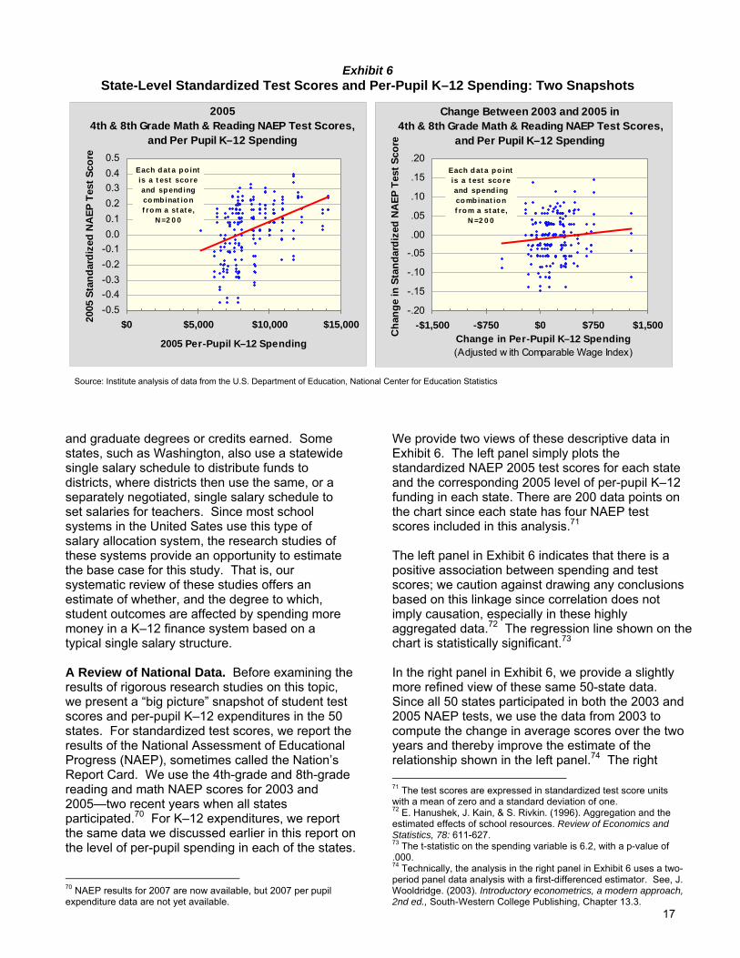
and graduate degrees or credits earned. Some states, such as Washington, also use a statewide single salary schedule to distribute funds to districts, where districts then use the same, or a separately negotiated, single salary schedule to set salaries for teachers. Since most school systems in the United Sates use this type of salary allocation system, the research studies of these systems provide an opportunity to estimate the base case for this study. That is, our systematic review of these studies offers an estimate of whether, and the degree to which, student outcomes are affected by spending more money in a K–12 finance system based on a typical single salary structure. A Review of National Data. Before examining the results of rigorous research studies on this topic, we present a “big picture” snapshot of student test scores and per-pupil K–12 expenditures in the 50 states. For standardized test scores, we report the results of the National Assessment of Educational Progress (NAEP), sometimes called the Nation’s Report Card. We use the 4th-grade and 8th-grade reading and math NAEP scores for 2003 and 2005—two recent years when all states participated.70 For K–12 expenditures, we report the same data we discussed earlier in this report on the level of per-pupil spending in each of the states.
70 NAEP results for 2007 are now available, but 2007 per pupil expenditure data are not yet available.
We provide two views of these descriptive data in Exhibit 6. The left panel simply plots the standardized NAEP 2005 test scores for each state and the corresponding 2005 level of per-pupil K–12 funding in each state. There are 200 data points on the chart since each state has four NAEP test scores included in this analysis.71 The left panel in Exhibit 6 indicates that there is a positive association between spending and test scores; we caution against drawing any conclusions based on this linkage since correlation does not imply causation, especially in these highly aggregated data.72 The regression line shown on the chart is statistically significant.73 In the right panel in Exhibit 6, we provide a slightly more refined view of these same 50-state data. Since all 50 states participated in both the 2003 and 2005 NAEP tests, we use the data from 2003 to compute the change in average scores over the two years and thereby improve the estimate of the relationship shown in the left panel.74 The right 71 The test scores are expressed in standardized test score units with a mean of zero and a standard deviation of one. 72 E. Hanushek, J. Kain, & S. Rivkin. (1996). Aggregation and the estimated effects of school resources. Review of Economics and Statistics, 78: 611-627. 73 The t-statistic on the spending variable is 6.2, with a p-value of .000. 74 Technically, the analysis in the right panel in Exhibit 6 uses a two-period panel data analysis with a first-differenced estimator. See, J. Wooldridge. (2003). Introductory econometrics, a modern approach, 2nd ed., South-Western College Publishing, Chapter 13.3.
Exhibit 6 State-Level Standardized Test Scores and Per-Pupil K–12 Spending: Two Snapshots
Source: Institute analysis of data from the U.S. Department of Education, National Center for Education Statistics
-0.5-0.4-0.3-0.2-0.10.00.10.20.30.40.5
$0 $5,000 $10,000 $15,000
2005 Per-Pupil K–12 Spending
2005
Sta
ndar
dize
d N
AEP
Tes
t Sco
re
20054th & 8th Grade Math & Reading NAEP Test Scores,
and Per Pupil K–12 Spending
Each dat a p o int is a t est sco re and sp end ing co mbinat io n f ro m a st at e,
N =2 0 0
-.20
-.15
-.10
-.05
.00
.05
.10
.15
.20
-$1,500 -$750 $0 $750 $1,500Change in Per-Pupil K–12 Spending(Adjusted w ith Comparable Wage Index)
Cha
nge
in S
tand
ardi
zed
NA
EP T
est S
core
Change Between 2003 and 2005 in 4th & 8th Grade Math & Reading NAEP Test Scores,
and Per Pupil K–12 Spending
Each d at a p o int is a t est sco re and spend ing co mb inat io n f ro m a st at e,
N =2 0 0
18
panel indicates only a slightly positive association between spending levels and test scores; however, once again we caution against any causal inference with these data.75 The important point from these two simple analyses is that there appears to be a small positive correlation between the levels of expenditures and student test score outcomes, although the relationship weakens as soon as some degree of statistical control is added to the estimates. A Systematic Review of Research Studies. This quick review of 50-state data shown in Exhibit 6 does not provide the quality of evidence needed to determine whether spending more money in typical K–12 funding structures causes an increase in test scores. That is, the previous simple analysis offers a correlational, but not a causal view of the evidence. To provide a causal interpretation, we are in the process of systematically reviewing the results of all studies we can locate that have addressed this basic question. To date we have analyzed the results of 69 studies; many of these, however, do not have sufficient methodological quality to be included in our analysis.76 In Exhibit 7 we plot the results of the 23 methodologically sound studies we have included in our formal review. These 23 studies contribute 49 tests of the degree to which money spent in a typical K–12 funding system affects student outcomes as measured by test scores or graduation rates.77 The results of the studies shown in Exhibit 7 reveal that most estimates have positive effect sizes and a few have negative effect sizes. A positive effect size means that, after controlling for other factors, a study found a positive linkage between spending money and improved student outcomes. While the results of many studies are positive, many are quite close to zero. The effect size metric for this analysis is the annual gain in test scores, in standard deviation units,
75 The t-statistic on the spending variable is 1.5 with a p-value of .136. The effect size measuring the annual gain in student test scores for a one-year 10 percent increase in spending is .012 standard deviation units. 76 For studies measuring the effect of K–12 expenditures on student outcomes, we generally excluded studies that were not value added (did not control for students’ prior test score) or did not control for student or school characteristics; studies using individual-level datasets were preferred over more aggregated datasets. 77 In this preliminary analysis, we have included all effects measured by each study. Therefore, some of these effects are not independent observations for this analysis. This issue will be addressed in our subsequent analysis.
for a 10 percent increase in per-pupil expenditures. The vertical red line in Exhibit 7 is our preliminary estimate of the expected effect based on the results of this group of studies.78 Our draft estimate is that a 10 percent increase in per-pupil expenditures produces a one-year gain of .007 standard deviation test score units. This effect, though small, is statistically significant.79
78 See Appendix A for details on these methods.
Exhibit 7 Draft Annual Impact of Increasing
Per-Pupil K–12 Expenditures by Ten Percent (Holding Other Factors Constant)
Effect Size (Annual gain, in standard deviation test score units,
How does this .007 effect size compare with the simple estimate obtained from the national data shown in Exhibit 6? The equivalent effect size for the relationship shown in the right panel of Exhibit 6 is .012. Thus, the best estimate from the review of higher quality studies (.007) is about 39 percent lower than the effect size from the simple estimate. This is a draft estimate; as the work of the Task Force proceeds, we will refine this estimate by including any additional methodologically sound studies not yet in our review and by estimating, if possible, the effect for subgroups, for different types of student tests (for example, math or reading), and for various grade levels. The first-cut estimate presented here is our preliminary overall effect. As noted earlier, effect sizes are not an intuitive metric for common understanding, although they are the main technical currency of educational researchers. To draw out the implications for Washington, we are developing a forecasting model that converts effect size estimates into more meaningful statewide policy-level outcomes. The motivation to develop this model stems from the Legislature’s general direction to the Institute to project the “expected effect of the investment made under the new funding structure.”80 We do not have a forecast of the base-case option for this report. When completed, we will produce a forecast of the general type shown in Exhibit 3, except that the projection will pertain to the effect sizes discussed in this section on the base-case option. While the forecast is not yet ready, we can present some back-of-the-envelope calculations of how Washington’s high school graduation rate could be affected by the average effect size reported in Exhibit 7. As noted earlier, the current on-time high school graduation rate, as calculated by OSPI, is 74.3 percent. If overall per-pupil K–12 expenditures were increased in Washington by 10 percent, then our preliminary forecast indicates that Washington’s current high school graduation rate could be raised by about 1.6 percentage points. This estimate assumes that an incoming
79 The results of our meta-analysis of these 49 effects indicate a mean effect size of .007, significant at p=.052. 80 E2SSB 5627, § 2(5)(b)
kindergarten student will benefit from 13 years of 10 percent higher real per-pupil expenditures.81 Under the same assumptions, if overall per-pupil K–12 expenditures were increased in Washington by 40 percent, then we would anticipate that after 13 years of these higher real expenditures the graduation probability would increase by about 4.9 percentage points. As noted, these calculations are preliminary and will change as subsequent work on the projection model is completed during 2008.
81 This 13-year figure assumes that estimated annual gains are linearly cumulative, an assumption we will address in 2008 as we refine the projection model. Our forecast also includes a parameter for the diminishing returns that can be anticipated as high school graduation rates are increased. See Appendix B for details.
20
The legislation requires the Institute to prepare a report on two to four options for school employee compensation. In the previous section, we presented a draft “base-case” option. The legislation also specifies that “one of the options must be a redirection and prioritization within existing resources based on research-proven education programs.” This second option can thus be called a “zero-based” option, since it must identify research-based approaches that can increase student outcomes within current funding levels. As noted in this report, the primary way certified school employees are paid in Washington is through a single salary schedule. A single salary schedule compensates school employees based on two factors: years of experience in the system and graduate degrees and/or credits earned. In Washington, the legislature adopts a single salary schedule that is used, along with other factors, to allocate funds to districts. At the district level, a single salary schedule is then separately negotiated to pay certified staff, subject to each district’s overall salary allocation factor. Many districts use the same single salary allocation schedule the state uses to distribute funds to districts. We have started our effort to prepare this zero-based option for the Task Force by examining the two main elements in the single salary schedule: years of experience and graduate degrees earned. We are systematically reviewing the results of all methodologically sound research studies that have addressed this basic question: Do teachers with more years of experience or graduate degrees improve the outcomes of their students more than teachers with less experience or without graduate degrees? Our work is not complete on these two topics; in this report we present preliminary findings. The results of our analyses to date are shown in Exhibits 8 and 9. Exhibit 8 depicts our draft findings on the effect of graduate degrees on student outcomes. Exhibit 9 displays our preliminary estimates of the effect of teacher experience on student outcomes.
Graduate Degrees. Thus far we have analyzed 13 studies with 34 separate effects that have examined the question of whether having a graduate degree (usually a master’s degree) improves the ability of a teacher to raise the academic performance of her or his students. In these studies, student academic performance is almost always measured by scores on reading or mathematics tests. Exhibit 8 plots the effect sizes we calculated from these studies. As can be observed, some studies have found positive effects, others negative effects, while many studies have found no effect.
Draft Analysis of a “Zero-Based” Option: Teacher Salary Allocations Based on Graduate Degrees and Experience
Exhibit 8 Draft Estimates of the Effect of Teachers With
Graduate Degrees on Student Outcomes
Effect Size (Annual gain in standard deviation test score units
from a teacher with a graduate degree)
-.100 -.075 -.050 -.025 .000 .025 .050 .075 .100
Harris & Sass (2007)
Harris & Sass (2007)
Harris & Sass (2007)
Harris & Sass (2007)
Ladd et al. (2007)
Clotfelter et al. (2006)
Rivkin et al. (2005)
Harris & Sass (2007)
Ladd et al. (2007)
Wenglinsky (1998)
Ladd et al. (2007)
Ladd et al. (2007)
Ladd et al. (2007)
Clotfelter et al. (2006)
Krieg (2006)
Hanushek (1992)
Goldhaber & Anthony (2007)
Ladd et al. (2007)
Eide & Showalter (1998)
Clotfelter et al. (2007)
Rivkin et al. (2005)
Ladd et al. (2007)
Goldhaber & Anthony (2007)
Ladd et al. (2007)
Aaronson et al. (2007)
Goldhaber & Brewer (1997)
Krieg (2006)
Hanushek (1992)
Krieg (2006)
Koedel & Betts (2007)
Wenglinsky (1997)
Krieg (2006)
Harris & Sass (2007)
Koedel & Betts (2007)
Average effect
21
We conclude from this draft analysis that there is no consistent relationship between teachers with graduate degrees and increased student outcomes as measured by test scores. Our average estimate, as shown by the vertical line in Exhibit 8 is essentially zero. It must be emphasized that this draft result needs refinement. In particular, the Institute will examine additional research literature addressing whether particular types of graduate degrees have impacts on student performance. For example, a relevant question is whether in-field or mathematics and science graduate degrees improve the effectiveness of teachers in particular fields.82 Teacher Experience. The picture that emerges for the effect of teacher experience is different than that for the effect of graduate degrees. Thus far, we have found 15 methodologically sound studies, with 42 measured effects, that have examined whether a teacher’s experience affects student outcomes. We plot the average effect sizes we have found to date in Exhibit 9. These results indicate that in the first few years on the job, a teacher gains considerably in her or his ability to improve the academic performance of students. The effect increases rapidly in years one to five and then begins to level off so that the marginal gains in effectiveness become smaller after these initial years of experience. National Board for Professional Teaching Standards (NBPTS) Certification. Another approach Washington has used in recent years to supplement teachers’ compensation is the NBPTS certificate.83 This is an element that could be included in a zero-based redirection of current resources based on research-based findings. We are currently reviewing methodologically sound studies on this topic. To date, we have identified four methodologically sound studies with 12 effects. Our analysis of these and additional studies will be presented to the Task Force in 2008.
82 See, for example, D. Goldhaber & D. Brewer. (1997). Why don’t schools and teachers seem to matter? Assessing the impact of unobservables on educational productivity. The Journal of Human Resources, 32(3): 505-523; A. Wayne & P. Youngs. (2003). Teacher characteristics and student achievement gains: A review. Review of Educational Research, 73(1):89-122. 83 See page 23 in this report for more information.
For a zero-based option, the implication of the two findings on graduate degrees and experience is that, within the context of the single salary schedule, academic performance would be improved by adjusting salary schedules to place more emphasis on experience and less (or no) emphasis on graduate degrees. Additional analyses need to be completed before constructing all of the components of a zero-based option. For example, in order to project the effect of a zero-based option on statewide student outcomes (as required in the legislation), supplemental analyses will need to be undertaken. For example, changing the reward structure for teachers would likely be phased in, thus decisions are necessary about “grandfathering” existing staff salaries. These refinements will be undertaken during 2008 as the work of the Task Force proceeds.
Exhibit 9 Draft Estimates of the Effect of
Years of Teacher Experience on Student Test Scores
Years of Teaching Experience
0.000.010.020.030.040.050.060.070.080.090.10
0 5 10 15 20
Effe
ct S
ize
Rel
ativ
e to
Tea
cher
With
No
Expe
rienc
e(s
tand
ard
devi
atio
n un
its)
22
As noted earlier in this report, the Legislature directed the Institute to analyze “at least two but no more than four options for allocating school employee compensation.”84 In the previous sections, we presented preliminary “base-case” and “zero-based” analyses as the first two options. In this section, we describe a number of other compensation-related options that have been part of policy discussions nationally and in Washington State. The enabling legislation directs the Task Force to consider several school employee compensation policies, including:
“Whether the compensation system for instructional staff shall include pay for performance, knowledge and skills elements;
Regional cost-of-living elements;85
Elements to recognize assignments that are difficult; and
Recognition for the professional teaching level certificate in the salary allocation model.” 86
These same topics were also covered in the recent Washington Learns process by its K–12 Advisory Committee,87 Finance Subcommittee,88 Compensation Subgroup,89 and the report by Odden and Picus.90 Some topics were discussed in the Conley study commissioned by the WEA91
84 E2SSB 5627 § 2(5)(b). 85 Cost-of-living adjustments were discussed earlier in this report and are not described in this section. For a summary of available methods, see L. Taylor & W. Fowler. (2006). A comparable wage approach to geographic cost adjustment. Washington, D.C.: Institute of Education Sciences, National Center for Education Statistics, U.S. Department of Education. 86 E2SSB 5627 § 3(2) 87 Washington Learns K–12 Advisory Committee. (June 6, 2006). Recommendations to the Washington Learns Committee. http://www.washingtonlearns.wa.gov/materials/ 060628_Bergeson_HunterTable.pdf 88 Washington Learns K–12 Advisory Committee, Finance Subcommittee. (August 22, 2006). Transparency and a vision for resources: Finance subcommittee recommendations for general apportionment, categorical programs, and local levy authority. http://www.washingtonlearns.wa.gov/materials/ Financeslides8-22w-ACchanges.pdf 89 Washington Learns K–12 Advisory Committee. (May 23, 3006). Compensation subgroup recommendations. http://www.washingtonlearns.wa.gov/materials/Compensation SubgroupRecommendationsFinal.pdf 90 Odden & Picus, 2006 91 Conley, 2007
and the 2004 House of Representatives K–12 Finance workgroup.92 Reforms in school employee compensation are under consideration in some locations in the U.S. and have been implemented in some states and districts. This section draws on recent summaries and reviews of these approaches by Dan Goldhaber,93 Susanna Loeb,94 Michael Podgursky,95 and Debbi Harris.96 Dr. Goldhaber, a consultant to the Institute on this project, offers the following overview of teacher pay reforms and the degree to which current research supports their implementation:
“Even though the research on teacher compensation reform is hardly definitive enough to recommend the use of specific pay reforms to reach specific goals, the few quantitative studies that do exist suggest that a more strategic use of teacher compensation could lead to both a more equitable allocation of teachers among students and increased student achievement.” 97
During 2008, as part of the Institute’s research for the Task Force, we will analyze the limited empirical research on these topics. The goal of this forthcoming analysis will be to identify promising approaches that can lead to “a more strategic use of teacher compensation” to improve student outcomes. For this report, we describe the four supplemental pay policy concepts in Goldhaber’s summary. Exhibit 10 on the following page lists the four key concepts relating to pay for: knowledge and skills, performance, hard-to-staff schools, and hard-to-staff subjects.
92 House Appropriations and Education Committees K–12 Finance Workgroup. (May 12, 2004). Overview of current salary structure and alternative compensation structures. http://www.leg.wa.gov/Documents/opr/k12finance/2004/ Compensation.pdf 93 D. Goldhaber. (2006). Teacher pay reforms: The political implications of recent research. Washington, D.C.: Center for American Progress. 94 S. Loeb. & L. Miller. (2006). A review of state teacher policies: What are they, what are their effects, and what are their implications for school finance? Stanford, CA: Institute for Research on Education Policy & Practice, School of Education, Stanford University. 95 M. Podgursky & M. Springer. (2006). Teacher performance pay: A review. Nashville: National Center on Performance Incentives, Vanderbilt University. 96 Harris, 2007 97 Goldhaber, 2006, p. 26
Draft Description of Other Compensation-Related Policy Options
23
Exhibit 10 Supplemental Pay Policy Concepts
Supplemental Pay …
For: Provided to: Based on: Knowledge and Skills
Individuals Completion of training, demonstration of particular skills, and/or assumption of increased responsibilities
Performance Individuals, Teams, and/or Schools
Student test scores (typically), teacher evaluations or other performance measures (less often)
Hard-to-Staff Schools
Individuals Teaching assignment in hard-to-staff schools
Hard-to-Staff Subjects
Individuals Teaching assignment in certain subjects (typically math and science)
Source: Institute review of Goldhaber, 2006; Loeb & Miller, 2006; Podgursky & Springer, 2006; and Harris, 2007.
Pay for Knowledge and Skills Systems of supplemental pay for knowledge and skills typically reward school employees for completion of specified training or demonstration of particular skills. In this approach, a standardized measure of performance, such as a state or national teaching certificate, is typically used to measure knowledge and skills. Teachers are awarded pay increases or bonuses as they achieve levels of certification or assume new responsibilities. Some examples follow. Professional Teacher Level Certificate. In recent years, Washington’s Professional Educator Standards Board (PESB) has proposed aligning the salary schedule with the knowledge- and skills-based professional level statewide teaching certificate.98,99 Under this proposal, the salary schedule would be altered to replace credit- and degree-based steps with teachers’ attainment of the state professional teaching certificate.
98 See for example: PESB. (2003). Getting and keeping the teachers we need: Paying for what we value, p. 6. http://www.pesb.wa.gov/Publications/Policybriefs/ Compensation.pdf 99 The certificate is described in detail at: http://www.k12.wa.us/certification/profed/ProfCertInfo.aspx
National Board for Professional Teaching Standards (NBPTS) Certification. NBPTS is a voluntary national teacher certification system. Thirty-seven states and D.C. compensate teachers for becoming NBPTS certified, either by supporting teachers during the process or by providing one-time or annual monetary bonuses (see Exhibit 11 on the following page for details).100 In 2007, Washington increased its NBPTS annual bonus from $3,500 to $5,000; this amount will be inflation-adjusted in fiscal year 2009.101 Career Ladder Programs. Another version of knowledge- and skills-based pay is a “career ladder” program, in which supplemental pay is linked to teachers’ assumption of additional responsibilities (such as taking on a mentoring role or serving on curriculum committees). Six states provide financial incentives for schools to implement career ladder programs: Arizona, Florida, Indiana, Missouri, Nevada, and Utah.102 An example of a pay for knowledge and skills career ladder system is Douglas County, Colorado. This district provides a bonus of $2,500 to “master teachers,” $1,250 to “outstanding teachers,” $700 to teachers taking on additional responsibilities, and $350 to teachers who complete specified skills training.103
100 Loeb & Miller, 2006, p. 46 101 HB 1128 § 113(41)(a)(i). Washington teachers may also apply for a scholarship to cover half of NBPTS fees ($1,250). 30 scholarships are awarded annually. http://www.k12.wa.us/ certification/nbpts/become.aspx#scholarships 102 Loeb & Miller, 2006, p. 52 103 Goldhaber, 2006, p. 13. These teachers are identified by a combination of education, training, portfolio evaluation, and analysis of their students’ test scores. For more information visit: http://www.dcsdk12.org/portal/page/portal/DCSD/Human_Resources/Certified_Staff/Pay_for_Performance
24
Exhibit 11 State Policy Incentives for NBPTS Certification
Type of Incentive Amount #
States States
One-time award or bonus
$1,500 to $5,000
6 AR, DC, HI, MT, ND, VA
Annual bonus $1,000 to $7,500
27 AL, AR, CA, DE, FL, GA, HI, ID, IL, IA, KS, KY, LA, MD, MA, MS, NV, NY, NC, OH, OK, SC, SD, VA, WA, WV, WI
No incentives 13 AK, AZ, CT, IN, MN, NE, NH, NM, OR, PA, TN, TX, UT
Source: Loeb & Miller (2006), p. 47 *See footnote 101 p. 23 Pay for Performance Pay for performance policies—sometimes referred to as “merit pay” programs—link part of educators’ salaries to specified outcomes, usually increases in student test scores. Pay for performance policies are the most frequently proposed, and most controversial, teacher pay policies in the United States.104 These policies are less controversial when whole schools or groups of teachers (rather than individual teachers) are evaluated and awarded bonuses or salary increases. Sometimes, teacher performance evaluations are used in place of or in addition to student achievement measures.105 School systems and states that have, or plan to implement, a pay for performance program include, but are not limited to, Florida, Houston,
104 Goldhaber, 2006, p. 12 105 Loeb & Miller, 2006, p. 50
the national Teacher Advancement Program, Minnesota, Denver, North Carolina, Texas, and Houston. Florida. Since 2006, Florida has provided state funding for districts to award performance pay to teachers and administrators.106 The bonuses are based on a combination of student test scores and teacher performance evaluations. At least 60 percent of the determination must be based on student state and national standardized test scores; up to 40 percent can be based on personnel evaluations. The amount of the award is calculated to be equal to 5 to 10 percent of average pay to the highest-paid teachers and administrators within each school district.107 The program is voluntary for those districts that choose to implement performance pay. Teacher Advancement Program (TAP). This national program provides grants for districts to award supplemental pay to teachers based on a combination of knowledge, skills, and performance-based elements: a career ladder, professional development, performance-based measures, and professional evaluation.108 TAP is a private program, separate from the U.S. Department of Education’s Teacher Incentive Fund (TIF).109 The amount of performance and career ladder TAP bonuses for individual teachers varies from $2,000 to $11,000.110 Minnesota (Quality Compensation for Teachers, or Q Comp). Minnesota’s Q Comp program, modeled after TAP, was created in 2005.111 Like Florida’s performance-pay model, Q Comp is voluntary (districts can choose 106 The program was created as the “Special Teachers Are Rewarded” (STAR) program in 2006 and reauthorized by the 2007 Legislature as the “Merit Award Program” (MAP). 107 Florida performance pay guidance 2007–2008 and beyond, p. 3. http://www.fldoe.org/PerformancePay/pdfs/MeritAwardProgram.pdf 108 This program was originally started by the Milken Family Foundation and is now part of the National Institute for Excellence in Teaching (NIET), a private entity that provides technical assistance to school districts implementing teacher quality reforms. According to the NIET website, TAP has been implemented in at least 36 school districts in 13 states. http://www.talentedteachers.org/about.taf?page=history 109 TIF was created by the U.S. Congress in 2006 as a discretionary grant program to provide grants to school districts that implement pay for performance programs in high-needs schools. In 2007, 34 grants were awarded to school districts, charter schools, consortia of districts and schools, and some statewide programs. For more information, visit: http://www.ed.gov/programs/teacherincentive/index.html 110 Podgursky & Springer, 2006, p. 10 111 The program replaced Minnesota’s “Alternative Compensation Teacher Pilot Program” that was originally implemented in 2002. http://www.wcer.wisc.edu/CPRE/conference/feb07/presentations/Anderson022107PM.ppt
25
whether to implement the program and receive the supplemental state funding). Local districts develop implementation details, including how performance is measured and what amount of school employee compensation is provided. Approved districts receive $190 per student in state funding and $70 per student in a partially equalized levy.112 Denver (ProComp). Denver Public Schools provides individual teachers with additional compensation based on a combination of: knowledge and skills (advanced degree), professional evaluation from administrators, assignments to hard-to-staff positions or hard-to-serve schools, and measures of student performance.113 Compensation amounts range from $330 to $7,582.114 North Carolina. North Carolina’s state-funded “ABCs of Public Education” program establishes benchmark and growth academic standards based on standardized test results. Schools that attain the standards are eligible for financial rewards. Depending on school-wide performance, certified staff receive $750 to $1,500 and teaching assistants $375 to $500.115 Texas has also recently created a state-funded school-wide performance incentive program (the “Educator Excellence Award Grant”). Schools are eligible for grants between $40,000 and $300,000, depending on the number of students enrolled. As in Minnesota, the Texas program provides local districts discretion regarding how to measure performance and how much supplemental pay is awarded to individuals within schools.116 Houston. In 2006, the Houston Independent School District (HISD) implemented performance pay using mostly district, and some federal, funding.117 Using a value-added model, the HISD awards individual teachers up to $7,300 based on increases in student standardized test scores. Awards are made in several ways: to individual
112 For more information, visit: http://education.state.mn.us/MDE/ Teacher_Support/QComp/index.html 113 See: http://denverprocomp.org 114 Podgursky & Springer, 2006, p. 7 115 Ibid. 116 See: http://www.tea.state.tx.us/opge/disc/EducatorExcellence Award/TEEG_overview.pdf 117 For the 2007–08 school year, the Houston School Board budgeted $23.1 million for the program, with $2.6 million provided by the federal Teacher Incentive Fund. http://www.houstonisd.org/ResearchAccountability/Home/Teacher%20Performance%20Pay/Teacher%20Performance%20Pay/Board%20Items/ASPIRE_Board_Approval.pdf
teachers, to teams of core teachers, to departments, and to entire schools.118 Pay for Hard-to-Staff Schools Policies in this category are designed to increase the quality of teachers in low-performing schools, because, as found by Loeb and Reininger, “[t]alented teachers are not distributed evenly across schools. In fact, there exists a systematic sorting of lesser-qualified teachers to high-poverty, low-performing schools.”119 This systematic disparity is found within, and not just among, school districts. Goldhaber found that “within districts, schools with less-desirable working conditions have no means to adjust their compensation, and, as a result, the most qualified teachers choose the more-affluent schools.”120 Six states, including Washington, provide a state salary bonus or differential as an incentive for teachers to work in hard-to-staff schools (see Exhibit 12). “Hard-to-staff” schools are usually defined as those with higher than average proportions of low-income students. In Washington, NBPTS teachers in schools with 70 percent or more students eligible for federal free and reduced price lunch get an additional $5,000 on top of the NBPTS bonus, annually.121 In addition to the six states listed in Exhibit 12, differential pay has been implemented within urban school districts. The Philadelphia School District provides teachers with an annual bonus of $2,000, and Palm Beach County, FL, $5,000.122 Virginia has a pilot program in two districts that provides a $15,000 one-time hiring bonus to teachers who agree to work in an identified hard-to-staff middle or high school.123
118 Principals are awarded up to $12,000 based on the same plan. These amounts apply to the 2007–08 school year. For more information visit: http://www.houstonisd.org/portal/site/Research Account ability/?vgnextoid=1eaa1d3c1f9ef010VgnVCM100000 28147fa6RCRD&vgnextfmt=default&epi_menuItemID=ce4a6ecb358c0d7fffa5a510e041f76a 119 S. Loeb & M. Reininger. (2004). Public policy and teacher labor markets: What we know and why it matters. East Lansing: The Education Policy Center at Michigan State University, p. 27. 120 D. Goldhaber, K. Destler, & D. Player. (2007). Teacher labor markets and the perils of using hedonics to estimate compensating differentials in the public sector. Seattle: School Finance Redesign Project, Center on Reinventing Public Education, University of Washington. p. 15 121 HB 1128 § 113(41)(a)(ii). Not adjusted for inflation. 122 Goldhaber, 2006, p. 16 123 Education Commission of the States http://mb2.ecs.org/reports/Report.aspx?id=1280
26
Exhibit 12 State Policy Incentives for Specific Job Assignments
Policy provides incentives to teach in:
States with salary differential
States with Other Benefits Tuition/fee support, loan assumption, housing, retirement benefits
Hard-to-Staff Schools
AK, CA, HI, NY, WA
AK, CA, CT, FL, HI, IL, KS, KY, LA, MD, MN, MS, NE, NM, NY, NC, OR, SC, TN, TX, UT, VA, WA, WV, WI
Hard-to-Staff Subjects
AL, CA, LA, NY
AL, AK, CA, CO, CT, DE, FL, GA, HI, IL, IN, IA, KS, KY, LA, ME, MD, MI, MS, MO, NM, NY, OK, OR, SC, TX, UT, VT, VA, WA, WV, WI, WY
Combinations (e.g., hard-to-staff subject in a low-income school)
CA, LA AK, CA, FL, IL, LA, MO, SC
Source: Loeb and Miller, 2006, Table A-13B, p. A-87 to A-88. Pay for Hard-to-Staff Subjects Another type of teacher pay incentive related to knowledge and skills is a subject-area differential. Under this type of policy, teachers in certain subjects—usually math and science—are paid more than teachers of other subjects. The rationale for such pay differentials is that “individuals with different attributes face different financial opportunity costs to enter the teacher labor market.”124 In other words, teachers in certain fields could make more money if they chose a different profession. Differential subject-area pay is intended to increase the incentive for these individuals to enter and remain in the teacher labor market. Some labor market research has found that teachers with technical degrees—particularly in math- and science-related fields—begin their careers earning average salaries comparable to individuals with the same degrees but who work in other employment sectors.125 However, over time, a gap between these teacher and non-teacher salaries emerges and increases. As they gain experience in the labor market, non-teachers in technical fields earn more than teachers with
124 D. Goldhaber, M. Armond, A. Liu, & D. Player. (2007). Returns to skill and teacher wage premiums: What can we learn by comparing the teacher and private sector labor markets? Seattle: School Finance Redesign Project, Center on Reinventing Public Education, University of Washington, p. 13. 125 Goldhaber, 2006
similar academic preparation. The average differential can be as high as $27,890 per year after 10 years of employment experience.126 In Washington, the PESB has identified statewide teacher shortage areas by subject, including math, science, special education, and English as a second language (ESL).127 The state currently does not allocate any supplemental compensation dollars to staff these subject areas. Exhibit 12 identifies four states that provide a subject-area differential for public school teachers: Alaska, California, Louisiana, and New York. Additionally, some school districts provide supplemental pay for hard-to-staff subject areas, including Houston ($5,000), Los Angeles ($5,000), and New York ($3,400).128 Exhibit 12 also shows that, for both hard-to-staff schools and subject-area policies, more states offer a non-salary benefit (e.g., tuition/fee support, loan assumption, housing, or retirement benefits) than a direct bonus or base salary increase. Some states offer both.
126 In comparison, for individuals with non-technical degrees, the average differential after ten years is estimated to be $18,904. Goldhaber, 2006, p. 8 127 The specific areas identified by the PESB for the 2007–09 biennium are: special education, English as a second language, chemistry, physics, science, mathematics, middle level math/science, early childhood special education, biology, and earth science. http://www.pesb.wa.gov/AlternativeRoutes/ AlternativeRoutes.asp 128 Goldhaber, 2006, p. 16
27
E2SSB 5627 directs the Institute to include in this report a “finalized timeline and plan for addressing the remaining components of a new funding system.”129 The legislative direction to the Institute is to propose “an initial timeline for a phased-in implementation of a new funding system that does not exceed six years.”130 The legislation is clear on the six-year implementation timeline. But, as staff to the Task Force, we cannot propose the specific phases of implementation until the Task Force has completed its responsibilities under the legislation—that is, to “develop options for a new funding structure and all necessary formulas.”131 Once the Task Force has accomplished this assignment, the specifics of a six-year timeline (as specified in the legislation) can be proposed. 129 E2SSB 5627, § 2(5)(b) 130 Ibid., § 2(5)(a) 131 Ibid., § 2(1)
The legislation also directs the Institute to discuss its research plan for addressing components in addition to school employee compensation. The legislation lists a number of these elements, including:
Professional development for all staff;
Voluntary all-day kindergarten;
Optimum class size, including different class sizes based on grade level and ways to reduce class size;
Focused instructional support for students and schools;
Extended school day and school year options; and
Health and safety requirements.132 Presently, the Institute is engaged in reviewing the research literature on these topics using the evidence-based methods described in this report. The Institute’s next report to the Task Force will be completed, as required in the legislation, on September 15, 2008.
132 Ibid., § 3(2)
Timeline and Plan
28
Exhibit 13 Citations to the Studies Used in Statistical Analyses
(Some studies contributed independent effect sizes from more than one location, grade level, or test type)
Teacher Effectiveness Aaronson, D., Barrow, L., & Sander, W. (2007). Teachers and student achievement in the Chicago public high schools. Journal of Labor Economics,
25(1), 95-135. Clotfelter, C. T., Ladd, H. F., & Vigdor, J. L. (2007, October). Teacher credentials and student achievement in high school: A cross-subject analysis with
student fixed effects. (Working Paper No. 11). Washington, DC: The Urban Institute, National Center for Analysis of Longitudinal Data in Education Research.
Goldhaber, D. D., & Brewer, D. J. (1997). Why don't schools and teachers seem to matter? Assessing the impact of unobservables on educational productivity. The Journal of Human Resources, 32(3), 505-523.
Hanushek, E. A. (1992). The trade-off between child quantity and quality. Journal of Political Economy, 100(1), 84-117. Kane, T. J., et al. (2007). What does certification tell us about teacher effectiveness? Evidence from New York City. Economics of Education Review,
doi:10.1016/j.econedurev.2007.05.005. Koedel, C., & Betts, J. R. (2007, April). Re-examining the role of teacher quality in the educational production function. Columbia: University of Missouri-
Columbia, Department of Economics. Krieg, J. M. (2006). Teacher quality and attrition. Economics of Education Review, 25(1), 13-27. Leigh, A. (n.d.). Estimating teacher effectiveness from two-year changes in students' test scores. Canberra, Australia: Australian National University,
Research School of Social Sciences. Murnane, R. J., & Phillips, B. R. (1981). What do effective teachers of inner-city children have in common? Social Science Research, 10(1), 83-100. Nye, B., Konstantopoulos, S., & Hedges, L. V. (2004). How large are teacher effects? Educational Evaluation and Policy Analysis, 26(3), 237-257. Rivkin, S. G., Hanushek, E. A., & Kain, J. F. (2005). Teachers, schools, and academic achievement. Econometrica, 73(2), 417-458. Rockoff, J. E. (2004). The impact of individual teachers on student achievement: Evidence from panel data. The American Economic Review, 94(2), 247-
252. Rowan, B., Correnti, R., & Miller, R. J. (2002). What large-scale, survey research tells us about teacher effects on student achievement: Insights from the
prospects study of elementary schools. Teachers College Record, 104(8), 1525-1567. Per-Pupil Expenditures (Base-Case Option) Deke, J. (2003). A study of the impact of public school spending on postsecondary educational attainment using statewide school district refinancing in
Kansas. Economics of Education Review, 22(3), 275-284. Eide, E., & Showalter, M. H. (1998). The effect of school quality on student performance: A quantile regression approach. Economics Letters, 58(3), 345-
350. Ferguson, R. F., & Ladd, H. F. (1996). How and why money matters: An analysis of Alabama schools. In H. F. Ladd (Ed.), Holding schools accountable:
Performance based reform in education (pp. 265–298). Washington, DC: Brookings Institution. Ferguson, R. F. (1991). Paying for public education: New evidence on how and why money matters. Harvard Journal on Legislation, 28(2), 465-498. Fuchs, T., & Wößmann, L. (2007). What accounts for international differences in student performance? A re-examination using PISA data. Empirical
Economics, 32(2), 433-464. Grimes, P. W. (1994). Public versus private secondary schools and the production of economic education. The Journal of Economic Education, 25(1), 17-
30. Grissmer, D. W., Flanagan, A., Kawata, J., & Williamson, S. (2000). Improving student achievement: What state NAEP test scores tell us. Santa Monica,
CA: RAND. Guryan, J. (2003, March). Does money matter? Estimates from education finance reform in Massachusetts (NBER Working Paper). Cambridge, MA:
National Bureau of Economic Research. Gyimah-Brempong, K., & Gyapong, A. O. (1991). Characteristics of education production functions: An application of canonical regression analysis.
Economics of Education Review, 10(1), 7-17. Hægeland, T., Raaum, O., & Salvanes, K. G. (2007, July). Pennies from heaven: Using exogenous tax variation to identify effects of school resources on
pupil achievement (Discussion Paper No. 508). Oslo, Norway: Statistics Norway, Research Department. Heinesen, E., & Graversen, B. K. (2005). The effect of school resources on educational attainment: Evidence from Denmark. Bulletin of Economic
Research, 57(2), 109-143. Kinnucan, H. W., Zheng, Y., & Brehmer, G. (2006). State aid and student performance: A supply-demand analysis. Education Economics, 14(4), 487-509. Levǎcić, R., Jenkins, A., Vignoles, A., Steele, F., & Allen, R. (2005). Estimating the relationship between school resources and pupil attainment at Key
Stage 3 (Research Report No. 679). London: Department for Education and Skills. Loeb, S., & Page, M. E. (2000). Examining the link between teacher wages and student outcomes: The importance of alternative labor market
opportunities and non-pecuniary variation. The Review of Economics and Statistics, 82(3), 393-408. Long, M. C. (2006). Secondary school characteristics and early adult outcomes (Working Paper No. 2006-06). Seattle: University of Washington, Daniel J.
Evans School of Public Affairs. Lopus, J. S. (1990). Do additional expenditures increase achievement in the high school economics class? Journal of Economic Education, 21(3), 277-
286. Papke, L. E. (2006). The effects of changes in Michigan's school finance system. East Lansing: Michigan State University, Department of Economics. Register, C. A., & Grimes, P. W. (1991). Collective bargaining, teachers, and student achievement. Journal of Labor Research, 12(2), 99-109. Ritzen, J. M., & Winkler, D. R. (1977). The revealed preferences of a local government: Black/white disparities in scholastic achievement. Journal of Urban
Economics, 4(3), 310-323. Sander, W. (1999). Endogenous expenditures and student achievement. Economics Letters, 64(2), 223-231. Taylor, C. (1998). Does money matter? An empirical study introducing resource costs and student needs to educational production function analysis. In
W. J. Fowler, Jr. (Ed.), Developments in school finance, 1997: Fiscal proceedings from the Annual State Data Conference (pp. 75-97). Washington, D.C.: U.S. Department of Education, National Center for Education Statistics.
Todd, P. E., & Wolpin, K. I. (2006, November). The production of cognitive achievement in children: Home, school and racial test score gaps. Philadelphia: University of Pennsylvania.
Wilson, K. (2001). The determinants of educational attainment: Modeling and estimating the human capital model and education production functions. Southern Economic Journal, 67(3), 518-551.
29
Exhibit 13 continued Citations to the Studies Used in Statistical Analyses
(Some studies contributed independent effect sizes from more than one location, grade level, or test type)
Teachers With Graduate Degrees Aaronson, D., Barrow, L., & Sander, W. (2007). Teachers and student achievement in the Chicago public high schools. Journal of Labor Economics,
25(1), 95-135. Clotfelter, C. T., Ladd, H. F., & Vigdor, J. L. (2006). Teacher-student matching and the assessment of teacher effectiveness. The Journal of Human
Resources, 41(4), 778-820. Clotfelter, C. T., Ladd, H. F., & Vigdor, J. L. (2007, October). Teacher credentials and student achievement in high school: A cross-subject analysis with
student fixed effects. (Working Paper No. 11). Washington, DC: The Urban Institute, National Center for Analysis of Longitudinal Data in Education Research.
Eide, E., & Showalter, M. H. (1998). The effect of school quality on student performance: A quantile regression approach. Economics Letters, 58(3), 345-350.
Goldhaber, D., & Anthony, E. (2007). Can teacher quality be effectively assessed? National board certification as a signal of effective teaching. The Review of Economics and Statistics, 89(1), 134-150.
Goldhaber, D. D., & Brewer, D. J. (1997). Why don't schools and teachers seem to matter? Assessing the impact of unobservables on educational productivity. The Journal of Human Resources, 32(3), 505-523.
Hanushek, E. A. (1992). The trade-off between child quantity and quality. Journal of Political Economy, 100(1), 84-117. Harris, D. N., & Sass, T. R. (2007, March). Teacher training, teacher quality and student achievement (Working Paper No. 3). Washington, DC: The Urban
Institute, National Center for Analysis of Longitudinal Data in Education Research. Koedel, C., & Betts, J. R. (2007, April). Re-examining the role of teacher quality in the educational production function. Columbia: University of Missouri-
Columbia, Department of Economics. Krieg, J. M. (2006). Teacher quality and attrition. Economics of Education Review, 25(1), 13-27. Ladd, H. F., Sass, T. R., & Harris, D. N. (2007, February). The impact of national board certified teachers on student achievement in Florida and North
Carolina: A summary of the evidence prepared for the National Academies Committee on the evaluation of the impact of teacher certification by NBPTS. Unpublished manuscript.
Rivkin, S. G., Hanushek, E. A., & Kain, J. F. (2005). Teachers, schools, and academic achievement. Econometrica, 73(2), 417-458. Wenglinsky, H. (1997). How money matters: The effect of school district spending on academic achievement. Sociology of Education, 70(3), 221-237. National Board Certification Cavalluzzo, L. C. (2004, November). Is national board certification an effective signal of teacher quality? Alexandria, VA: The CNA Corporation. Clotfelter, C. T., Ladd, H. F., & Vigdor, J. L. (2007, October). Teacher credentials and student achievement in high school: A cross-subject analysis with
student fixed effects. (Working Paper No. 11). Washington, DC: The Urban Institute, National Center for Analysis of Longitudinal Data in Education Research.
Goldhaber, D., & Anthony, E. (2007). Can teacher quality be effectively assessed? National board certification as a signal of effective teaching. The Review of Economics and Statistics, 89(1), 134-150.
Ladd, H. F., Sass, T. R., & Harris, D. N. (2007, February). The impact of national board certified teachers on student achievement in Florida and North Carolina: A summary of the evidence prepared for the National Academies Committee on the evaluation of the impact of teacher certification by NBPTS. Unpublished manuscript.
Years of Teaching Experience Aaronson, D., Barrow, L., & Sander, W. (2007). Teachers and student achievement in the Chicago public high schools. Journal of Labor Economics,
25(1), 95-135. Akerhielm, K. (1995). Does class size matter?. Economics of Education Review, 14(3), 229-241. Borland, M. V., Howsen, R. M., & Trawick, M. W. (2005). An investigation of the effect of class size on student academic achievement. Education
Economics, 13(1), 73-83. Boyd, D., Lankford, H., Loeb, S., Rockoff, J., & Wyckoff, J. (2007, September). The narrowing gap in New York City teacher qualifications and its
implications for student achievement in high-poverty schools (Working Paper No. 10). Washington, DC: The Urban Institute, National Center for Analysis of Longitudinal Data in Education Research.
Clotfelter, C. T., Ladd, H. F., & Vigdor, J. L. (2006). Teacher-student matching and the assessment of teacher effectiveness. The Journal of Human Resources, 41(4), 778-820.
Clotfelter, C. T., Ladd, H. F., & Vigdor, J. L. (2007, October). Teacher credentials and student achievement in high school: A cross-subject analysis with student fixed effects. (Working Paper No. 11). Washington, DC: The Urban Institute, National Center for Analysis of Longitudinal Data in Education Research.
Goldhaber, D., & Anthony, E. (2007). Can teacher quality be effectively assessed? National board certification as a signal of effective teaching. The Review of Economics and Statistics, 89(1), 134-150.
Goldhaber, D. D., & Brewer, D. J. (1997). Why don't schools and teachers seem to matter? Assessing the impact of unobservables on educational productivity. The Journal of Human Resources, 32(3), 505-523.
Harris, D. N., & Sass, T. R. (2007, March). Teacher training, teacher quality and student achievement (Working Paper No. 3). Washington, DC: The Urban Institute, National Center for Analysis of Longitudinal Data in Education Research.
Jepsen, C. (2005). Teacher characteristics and student achievement: Evidence from teacher surveys. Journal of Urban Economics, 57(2), 302-319. Kane, T. J., et al. (2007). What does certification tell us about teacher effectiveness? Evidence from New York City. Economics of Education Review,
doi:10.1016/j.econedurev.2007.05.005. Krieg, J. M. (2006). Teacher quality and attrition. Economics of Education Review, 25(1), 13-27. Ladd, H. F., Sass, T. R., & Harris, D. N. (2007, February). The impact of national board certified teachers on student achievement in Florida and North
Carolina: A summary of the evidence prepared for the National Academies Committee on the evaluation of the impact of teacher certification by NBPTS. Unpublished manuscript.
Rivkin, S. G., Hanushek, E. A., & Kain, J. F. (2005). Teachers, schools, and academic achievement. Econometrica, 73(2), 417-458. Rockoff, J. E. (2004). The impact of individual teachers on student achievement: Evidence from panel data. The American Economic Review, 94(2), 247-
252.
31
Appendix A: Effect Size Procedures This technical appendix describes the study coding criteria and the procedures for calculating effect sizes that we use in the Institute’s analysis of K–12 educational programs and services. In recent years, researchers have developed a set of statistical tools to facilitate systematic reviews of evaluation evidence. The set of procedures is called “meta-analysis” and we employ this methodology in our study.133 A1. Study Selection and Coding Criteria A meta-analysis is only as good as the selection and coding criteria used to conduct the study. The following are key coding criteria for our meta-analysis of evaluations of K–12 educational programs and services. 1) Study Search and Identification Procedures. We
search for all K–12 evaluation studies written in English. We use three primary sources: (a) study lists in other reviews of the K–12 research literature; (b) citations in individual evaluation studies; and (c) research databases/search engines such as Google, Proquest, Ebsco, ERIC, and SAGE.
2) Peer-Reviewed and Other Studies. Many K–12 evaluation studies are published in peer-reviewed academic journals, while others are from government or other reports. It is important to include non-peer reviewed studies, because it has been suggested that peer-reviewed publications may be biased toward positive program effects. Therefore, our meta-analysis includes studies regardless of their source.
3) Review of a Study’s Research Methodology. We examine each potential study to ascertain whether the study’s research design and data allow it to identify causal effects of a program or policy on an educational outcome.134 We include true experimental studies and other non-experimental or observational studies that have plausibly addressed the endogeneity problem inherent in K–12 educational studies. Econometric approaches to identify causal effects include instrumental variables regression, regression discontinuity designs, and fixed effects panel models. Some multivariate correlational designs employing hierarchical linear models, ordinary least squares regression, and matching designs are included if they have used a sufficient set of right-hand side controls.
133 We follow the meta-analytic methods described in M. Lipsey, & D. Wilson. (2001). Practical meta-analysis. Thousand Oaks: Sage Publications. 134 D. Webbink. (2005). Causal effects in education. Journal of Economic Surveys, 19(4): 535-560.
We do not include studies with a single-group, pre-post research design. We believe that it is only through rigorous comparison group studies that average treatment effects can be reliably estimated.135 For the regression studies in this review, we generally excluded studies that were not value added (did not control for students’ prior test score) or did not control for student or school characteristics; studies using individual-level datasets were preferred over more aggregated datasets.
4) Enough Information to Calculate an Effect Size. Following the statistical procedures in Lipsey and Wilson (2001), a study must provide the necessary statistical information to calculate an effect size. If such information is not provided, we attempt to contact the author of the study. If this effort still does not produce results, then we drop the study from our review.
5) Mean Difference Effect Sizes. For this study we are coding mean difference effect sizes following the procedures in Lipsey and Wilson (2001).
6) Unit of Analysis. Our unit of analysis is an independent test of treatment at a particular site or grade level.
7) Multivariate Results Preferred. Some studies present two types of analyses: raw outcomes that are not adjusted for covariates, such as family income and ethnicity; and those that are adjusted with multivariate statistical methods. In these situations, we code the multivariate outcomes.
8) Outcome Measures of Interest. We include studies that report student-level outcomes. The majority of studies report on student test scores. We also include studies that measure high school graduation/drop out, post-secondary education, and workforce participation. We exclude studies where the only outcomes are subjective opinions, such as teacher or parent satisfaction.
9) Some Special Coding Rules for Effect Sizes. Most studies that meet the criteria for inclusion in our review have sufficient information to code exact mean difference effect sizes. Some studies report some, but not all, of the information required. The rules we follow for these situations are as follows:
a) Two-Tail P-Values. Sometimes, studies only report p-values for significance testing of program
135 See: Identifying and implementing education practices supported by rigorous evidence: A user friendly guide. (2003, December). Coalition for Evidence-Based Policy, U.S. Department of Education, Institute of Education Sciences, National Center for Education Evaluation and Regional Assistance. Available at: http://www.evidencebasedpolicy.org/docs/Identifying_and_Implementing_Educational_Practices.pdf
Appendices
Appendix A: Effect Size Procedures A1: Study Selection and Coding Criteria A2: Procedures for Calculating Effect Sizes
Appendix B: Methods to Estimate the Impact of Educational Options on High School Graduation Appendix C: E2SSB 5627
32
outcomes. If the study reports a one-tail p-value, we will convert it to a two-tail test.
b) Declaration of Significance by Category. Some studies report results of statistical significance tests in terms of categories of p-values, such as p<=.01, p<=.05, or “not significant at the p=.05 level.” We calculate effect sizes in these cases by using the highest p-value in the category; e.g., if a study reports significance at “p<=.05,” we calculate the effect size at p=.05. This is the most conservative strategy. If the study simply states a result was “not significant,” we compute the effect size assuming a p-value of .50 (i.e. p=.50).
A2. Procedures for Calculating Effect Sizes Effect sizes measure the degree to which a program has been shown to change an outcome for program participants relative to a comparison group. There are several methods used by meta-analysts to calculate effect sizes, as described in Lipsey and Wilson (2001). In this analysis, we use statistical procedures to calculate standardized mean difference effect sizes of programs. We do not use the odds-ratio effect size because many of the outcomes measured in this study, such as test scores, are continuously measured. A mean difference effect size involves continuous data where the differences are in the means of an outcome.136
(A1)
2
2c
2t
ctm
SDSD
MMES+
−=
In this formula, ESm is the estimated effect size for the difference between means obtained from the information in a research study; Mt is the mean value of an outcome for the treatment or experimental group; Mc is the mean value of an outcome for the control group; SDt is the standard deviation of the mean for the treatment group; and SDc is the standard deviation of the mean for the control group. Often, Mt - Mc is obtained from coefficients in regression equations. Some research studies report the mean values needed to compute ESm in (A1), but they fail to report the standard deviations. In these cases, if the authors report statistical tests or confidence intervals, then this information allows the pooled standard deviation to be estimated. These procedures are described in Lipsey and Wilson (2001). Some of the outcomes we record are measured as dichotomies; for example, high school graduation. For these yes/no outcomes, Sanchez-Meca, et al.137 have shown that the Cox transformation produces the most unbiased approximation of the standardized mean effect size. We calculate the effect size for dichotomous outcomes using the formula: (A2) 65.1/)(ORLNESES Coxm =≅
136 Lipsey & Wilson, 2001, Table B10, equation 22, p. 200 137 J. Sanchez-Meca, F. Marin-Martinez, & S. Chacon-Moscoso. (2003). Effect-size indices for dichotomized outcomes in meta-analysis. Psychological Methods, 8(4): 448-467.
where OR is the odds ratio of success for the treatment group compared to the control group. The ESCox has a variance of
(A3) ⎥⎦
⎤⎢⎣
⎡+++=
CCEECox OOOO
xVar2121
1111367.0
where O1E, O2E, O1C, and O2C are the number of successes and failures (1s and 2s) in the treatment and control groups (E and C.) Adjusting Effect Sizes for Small Samples. In the group of studies considered in this review, there are no small samples. In our other work, some studies have very small sample sizes. In those cases, we follow the recommendation of many meta-analysts and adjust for this. Small sample sizes have been shown to upwardly bias effect sizes, especially when samples are less than 20. Following Hedges,138 Lipsey and Wilson139 report the “Hedges correction factor,” which we use to adjust all mean difference effect sizes (N is the total sample size of the combined treatment and comparison groups):
(A4) [ ]mm ESN
E ×⎥⎦⎤
⎢⎣⎡
−−=′
9431S
Adjusting Effect Sizes and Variances for Multi-Level Data Structures. Most studies in the education field use data that are hierarchical in nature. That is, students are clustered in classrooms, classrooms are clustered in schools, schools are clustered in districts, and districts are clustered in states. Analyses that do not account for clustering will underestimate the variance at the student level and thus may over-estimate effect sizes. In studies that do not account for clustering, effect sizes and their variance require additional adjustments. 140 There are two types of studies, each requiring a different set of adjustments.141 First, for student-level studies that ignore the variance due to clustering, we make adjustments to the mean effect size and its variance,
(A5) ( )2
121−−
−∗=NnESES mT
ρ
138 L. Hedges. (1981). Distribution theory for Glass’s estimator of effect size and related estimators. Journal of Educational Statistics, 6: 107-128. 139 Lipsey & Wilson (2001), equation 3.22, p. 49. 140 Studies that employ hierarchical linear modeling, or fixed effects with robust standard errors, or random effects models account for variance and need no further adjustment. 141 These formulas are taken from: L. Hedges. (In press). Effect sizes in cluster-randomized designs. Journal of Educational and Behavioral Statistics. DOI:10.3102/1076998606298043. Accessed November 27, 2007 at: http://jeb.sagepub.com/cgi/content/ abstract/1076998606298043v1
33
(A6)
{ } ( )( )
( )( ) ( ) ( ) ( )( ) ( ) ( )[ ] ⎟
⎟
⎠
⎞
⎜⎜
⎝
⎛
−−−−−−+−+−−
+−+⎟⎟⎠
⎞⎜⎜⎝
⎛ −=
ρρρρρ
ρ
12222122212
11
222
nNNnNnNnNES
nNN
NNESV
m
ct
ctT
Κ
Κ
where ρ is the intraclass correlation, the ratio of the variance between clusters to the total variance; N is the total number of individuals in the treatment group, Nt , and the comparison group, Nc; and n is the average number of persons in a cluster, K. In the educational field, clusters can be classes, schools, or districts. For this study, we used 2006 Washington Assessment of Student Learning (WASL) data to calculate values of ρ for the school-level (ρ = 0.114) and the district-level (ρ = 0.052). Class-level data are not available for the WASL, so we use a value of ρ = 0.200 for class-level studies. Second, for studies that report means and standard deviations at a cluster level, we make adjustments to the mean effect size and its variance:
(A7) ( ) ρρ
ρ∗
−+∗=
nnESES mT
11
(A8)
{ } [ ] ρρ
ρρ
ρ∗
⎪⎭
⎪⎬⎫
⎪⎩
⎪⎨⎧
−+∗−+
+⎟⎟⎠
⎞⎜⎜⎝
⎛ −+∗⎟⎟⎠
⎞⎜⎜⎝
⎛ −=
)2(2)1(1)1(1 2
ctm
ctct
T KKnESn
nn
KKKKESV
We did not adjust effect sizes in studies reporting dichotomous outcomes. This is because the Cox transformation assumes the entire normal distribution at the student level.142 Computing Weighted Average Effect Sizes, Confidence Intervals, and Homogeneity Tests. Once effect sizes are calculated for each program effect, and any necessary adjustments for clustering are made, the individual measures are summed to produce a weighted average effect size for a program area. We calculate the inverse variance weight for each program effect and these weights are used to compute the average. These calculations involve three steps. First, the standard error, SET of each mean effect size is computed with:143
(A9) )(2
)( 2
ctT
ctct
T NNES
NNNNSE
++
+=
Next, the inverse variance weight w is computed for each mean effect size with:144
(A10) 21
TSEw =
142 Mark Lipsey, personal communication, November 11, 2007. 143 Lipsey & Wilson (2001), equation 3.23, p. 49. 144 Ibid., equation 3.24, p. 49.
The weighted mean effect size for a group with i studies is computed with:145 (A11)
∑∑
=i
Tiw
ESwES i
)(
Confidence intervals around this mean are then computed by first calculating the standard error of the mean with:146 (A12)
∑=
iES w
SE 1
Next, the lower, ESL, and upper limits, ESU, of the confidence interval are computed with:147 (A13) )()1( ESL SEzESES α−−=
(A14) )()1( ESU SEzESES α−+=
In equations (A8) and (A9), z(1-α) is the critical value for the z-distribution (1.96 for α = .05). The test for homogeneity, which provides a measure of the dispersion of the effect sizes around their mean, is given by:148
(A15) ∑ ∑∑−=
i
iiiii w
ESwESwQ
22 )()(
The Q-test is distributed as a chi-square with k-1 degrees of freedom (where k is the number of effect sizes). Computing Random Effects Weighted Average Effect Sizes and Confidence Intervals. When the p-value on the Q-test indicates significance at values of p less than or equal to .05, a random effects model is performed to calculate the weighted average effect size. This is accomplished by first calculating the random effects variance component, v.149 (A16)
)()1(
∑∑∑ −−−
=iii
iwwsqw
kQv
This random variance factor is then added to the variance of each effect size and finally all inverse variance weights are recomputed, as are the other meta-analytic test statistics.
145 Ibid., p. 114 146 Ibid. 147 Ibid. 148 Ibid., p. 116 149 Ibid., p. 134
34
Appendix B: Methods to Estimate the Impact of Educational Options on High School Graduation This technical appendix describes our current model to compute estimates of how various educational options might affect high school graduation rates. We use effect sizes, derived mostly from student test scores, to estimate future high school graduation rates. To do this we calculate the marginal effect of a one standard deviation increase in test scores on high school graduation. We derive this relationship from two data sources:
• 10th-grade WASL scores for the graduating class of 2005
• 8th-grade combined math and reading scores from the National Educational Longitudinal Study150 (NELS88) of a representative sample of 8th-graders in 1988.
Scores were converted to z-scores with mean zero and standard deviation of one. In both data sets, we use logistic regression models to determine the effect of test scores on graduation, controlling for race, eligibility for free or reduced lunch, English as a second language status, sex, and disability. Logistic coefficients were: for WASL math, 1.068; for WASL reading, 0.972; for combined math and reading in NELS88, 0.968. For our models, we assumed a logistic coefficient of 1.00, the average of these three. Marginal effects were calculated according to the formula151 (B1) )1( YYME −= β Where ME is the marginal effect (the change in high school graduation percentage), β is the logistic coefficient for the relationship between test scores and graduation rates, and Y is the high school graduation rate prior to implementing an educational option. Our models for Washington assume Washington’s current graduation rate of 74.3 percent for all students and 64.8 percent for low-income students.152 We model the effects separately for low-income and non-low-income students, because the base rates for these two groups are dissimilar. The model assumes the educational option will be implemented for each year of school from kindergarten through 12th grade, and that the effects are cumulative, year after year, over the course of a student’s schooling.
150 Public use data set, National Education Longitudinal Study: 1988-1994 Data Files and Electronic Codebook System. U.S. Department of Education, National Center for Education Statistics. 151 R. Ramanathan. (1998). Introductory econometrics with applications, fourth edition. Fort Worth: The Dryden Press, Harcourt Brace College Publishers, Table 6.1, p. 257. 152 Ireland, 2006
The model also assumes diminishing returns of effect sizes. That is, as effects accumulate over time and base rates for graduation increase, we would expect the educational options would have smaller effects. For this analysis, we assume a 10 percent reduction in effect size for each 1 percent increase in graduation rates. That is, (B2) 1dim)1( −−×= y
y ESES Where ESy represents the expected value of the effect size after y years of implementation, ES is the effect size from our meta-analysis, and dim is the annual rate of decay in the effect size. We forecast the overall effect of an option by summing effects for each graduating class, assuming the state could fully implement an option in the school year 2007–08. Each subsequent graduating class would receive additional years of an option. So, for example, the effect would be small for the class of 2008, because they would receive only a single year of the option. On the other hand, the effects would be larger for children in kindergarten in 2007–08 who would have had the influence of 13 years of an educational option by graduation in 2020. For each year after implementation, we take a weighted average of estimated graduation for low-income and non-low-income students to arrive at a projected statewide graduation rate. In this version of the model, we assume the effects of multi-year educational options are linearly cumulative for students. In future versions, we will model the possibility that the effects do not accumulate linearly.
35
APPENDIX C: E2SSB 5627 AN ACT Relating to basic education funding.
Section 1. The state's definition of basic education and the corresponding funding formulas must be regularly updated in order to keep pace with evolving educational practices and increasing state and federal requirements and to ensure that all schools have the resources they need to help give all students the opportunity to be fully prepared to compete in a global economy. The work of Washington learns steering committee and the K–12 advisory committee provides a valuable starting point from which to evaluate the current educational system and develop a unique, transparent, and stable educational funding system for Washington that supports the goals and the vision of a world-class learner-focused K–12 educational system that were established in the final Washington learns report. This act is intended to make provision for some significant steps towards a new basic education funding system and establishes a joint task force to address the details and next steps beyond the 2007-2009 biennium that will be necessary to implement a new comprehensive K–12 finance formula or formulas that will provide Washington schools with stable and adequate funding as the expectations for the K–12 system continue to evolve. Section 2. (1) The joint task force on basic education finance established under this section, with research support from the Washington state institute for public policy, shall review the definition of basic education and all current basic education funding formulas, develop options for a new funding structure and all necessary formulas, and propose a new definition of basic education that is realigned with the new expectations of the state's education system as established in the November 2006 final report of the Washington learns steering committee and the basic education provisions established in chapter 28A.150 RCW. (2) The joint task force on basic education finance shall consist of fourteen members: (a) A chair of the task force with experience with Washington finance issues including knowledge of the K–12 funding formulas, appointed by the governor;(b) Eight legislators, with two members from each of the two largest caucuses of the senate appointed by the president of the senate and two members from each of the two largest caucuses of the house of representatives appointed by the speaker of the house of representatives; (c) A representative of the governor's office or the office of financial management, designated by the governor;(d) The superintendent of public instruction or the superintendent's designee; and (e) Three individuals with significant experience with Washington K–12 finance issues, including the use and application of the current basic education funding formulas, appointed by the governor. Each of the two largest caucuses of the house of representatives and the senate may submit names to the governor for consideration. (3) In conducting research directed by the task force and developing options for consideration by the task force, the Washington state institute for public policy shall consult with stakeholders and experts in the field. The institute may also request assistance from the legislative evaluation and accountability program committee, the office of the superintendent of public instruction, the office of financial management, the house office of program research, and senate committee services. (4) In developing recommendations, the joint task force shall review and build upon the following:(a) Reports related to K–12 finance produced at the request of or as a result of the Washington learns study, including reports completed for or by the K–12 advisory committee;(b) High-quality studies that
are available; and (c) Research and evaluation of the cost-benefits of various K–12 programs and services developed by the institute as directed by the legislature in section 607(15), chapter 372, Laws of 2006. (5) The Washington state institute for public policy shall provide the following reports to the joint task force: (a) An initial report by September 15, 2007, proposing an initial plan of action, reporting dates, timelines for fulfilling the requirements of section 3 of this act, and an initial timeline for a phased-in implementation of a new funding system that does not exceed six years; (b) A second report by December 1, 2007, including implementing legislation as necessary, for at least two but no more than four options for allocating school employee compensation. One of the options must be a redirection and prioritization within existing resources based on research-proven education programs. The report must also include a projection of the expected effect of the investment made under the new funding structure. The second report shall also include a finalized timeline and plan for addressing the remaining components of a new funding system; and (c) A final report with at least two but no more than four options for revising the remaining K–12 funding structure, including implementing legislation as necessary, and a timeline for phasing in full adoption of the new funding structure. The final report shall be submitted to the joint task force by September 15, 2008. One of the options must be a redirection and prioritization within existing resources based on research-proven education programs. The final report must also include a projection of the expected effect of the investment made under the new funding structure. Section 3. (1) The funding structure alternatives developed by the joint task force under section 2 of this act shall take into consideration the legislative priorities in this section, to the maximum extent possible and as appropriate to each formula. (2) The funding structure should reflect the most effective instructional strategies and service delivery models and be based on research-proven education programs and activities with demonstrated cost benefits. In reviewing the possible strategies and models to include in the funding structure the task force shall, at a minimum, consider the following issues: (a) Professional development for all staff; (b) Whether the compensation system for instructional staff shall include pay for performance, knowledge, and skills elements; regional cost-of-living elements; elements to recognize assignments that are difficult; recognition for the professional teaching level certificate in the salary allocation model; and a plan to implement the pay structure; (c) Voluntary all-day kindergarten; (d) Optimum class size, including different class sizes based on grade level and ways to reduce class size; (e) Focused instructional support for students and schools; (f) Extended school day and school year options; and (g) Health and safety requirements. (3) The recommendations should provide maximum transparency of the state's educational funding system in order to better help parents, citizens, and school personnel in Washington understand how their school system is funded. (4) The funding structure should be linked to accountability for student outcomes and performance. Section 4. This act is necessary for the immediate preservation of the public peace, health, or safety, or support of the state government and its existing public institutions, and takes effect immediately.
Document No. 07-12-2201
Washington State Institute for Public Policy
The Washington State Legislature created the Washington State Institute for Public Policy in 1983. A Board of Directors—representing the legislature, the governor, and public universities—governs the Institute and guides the development of all activities. The Institute’s mission is to carry out practical research, at legislative direction, on issues of importance to Washington State.