82
Representation of Convective Processes in NWP Models (part II) George H. Bryan NCAR/MMM Presentation at ASP Colloquium, “The Challenge of Convective Forecasting” 13 July 2006
| Date post: | 31-Dec-2015 |
| Category: |
Documents |
| Upload: | veda-everett |
| View: | 28 times |
| Download: | 1 times |

Representation of Convective Processes in NWP Models
(part II)
George H. Bryan
NCAR/MMM
Presentation at ASP Colloquium,
“The Challenge of Convective Forecasting”
13 July 2006

Outline
• Part I: What is a numerical model?
• Part II: What resolution is needed to simulate convection in numerical models?

Part II: What resolution is needed to simulate convection
in numerical models?
• An interesting question.
• What do our commandments say?

6. Thou shalt use 1 km grid spacing to simulate convection explicitly
7. ….
Commandments (continued)

6. Thou shalt use 1 km grid spacing to simulate explicitly convection
7. Honor thy elders
8. ….
Commandments (continued)
“There’s no need for grid spacing smaller than 2 km.”

Perspectives on resolution
• Historical Perspective
• Theoretical Perspective
• Pragmatic Perspective

1 10 100 km
Cumulus ParameterizationResolved Convection
LES PBL Parameterization
Two Stream Radiation3-D Radiation
Model Physics in High Resolution NWP
PhysicsŅNo ManÕs LandÓ

The “1 km standard”
• Often quoted in journal articles, textbooks, at conferences, etc.
• Clearly, there is some veracity to this “rule of thumb”– otherwise, it wouldn’t be so common
• But, where did it come from?

The first cloud models• Steiner (1973)
– Perhaps first 3D simulation of convection = 200 m– Cumulus congestus
• Schlesinger (1975)– Perhaps first 3D simulation of deep convection = 3.2 km– “a rather coarse mesh was used”
• Schlesinger (1978) = 1.8 km

The first cloud models (cont.)• Klemp and Wilhelmson (1978)
– A groundbreaking paper – The KW Model is the grand-daddy of the ARW
Model = 1 km– “… this resolution is admittedly rather coarse”
• Tripoli and Cotton (1980) = 750 m
• Weisman and Klemp (1982) = 2 km– “Finer resolution would be preferable …”

8. Thou shalt read the Old Testament
9. ….
Commandments (continued)

The first cloud models (cont.)• Klemp and Wilhelmson (1978)
– A groundbreaking paper – The KW Model is the grand-daddy of the ARW
Model = 1 km– “… this resolution is admittedly rather coarse”
• Tripoli and Cotton (1980) = 750 m
• Weisman and Klemp (1982) = 2 km– “Finer resolution would be preferable …”

Summary of literature review
of O(1 km) was there from the beginning
• Many recognized/suggested that this was too coarse
• In the decades that followed (80s and 90s), increasing computing power was utilized mainly for larger domains and longer integration times

Justification for 1 km
• Not a great deal of justification out there, other than:– The Sixth Commandment– “scientist A used this resolution; thus, I can,
too.”– “It’s all I could afford.”
• However …

Justification for 1 km
• Weisman et al. (1997) performed a large number of simulations, using from 12 km to 1 km– “… 4 km grid spacing may be sufficient to
reproduce … midlatitude type convective systems”
• They identified (correctly) that non-hydrostatic processes cannot be resolved unless 1 km

Weisman, Skamarock, and Klemp, 1997: The Resolution Dependence of Explicitly Modeled
Convective Systems (MWR, pg 527)
~4 km is sufficient to simulate mesoscale convective systems
System-averaged rainwater mixing ratio (qr)weak shear strong shear
higher resolution
“Clearly, the 1-km solution has not converged.”
higher resolution
“…grid resolutions of 500 m or less may be needed to properly resolve the cellular-scale features …”

Looking beyond 1 km
• Only since the middle 90s have people looked below 1 km systematically
• It’s expensive!– Need grids of O(1000 x 1000)– Small time steps
• Droegemeier et al. (1994, 1996, 1997)– Found differences in simulations of
supercells with 100 m
– Turbulent details began to emerge

from: Droegemeier et al. (1994)
Supercell simulations: rainwater mixing ratio at z = 4 km, t = 1 h

Other recent studies
• Petch and Grey (2001)• Petch et al. (2002)• Adlerman and Droegemeier (2002)• Bryan et al. (2003)• All found that results were not converged
with = 1 km – i.e., results are dependent on grid spacing– But why?– And what are consequences of coarse
resolution?

Δx = Δz = 125 m:
Δ x = 1000 m, Δz = 500 m:
θe, across-line cross sections
with RKW “optimal” shear

θe, along-line cross sections
with RKW “optimal” shear
Δx = Δz = 125 m:
Δ x = 1000 m, Δz = 500 m:
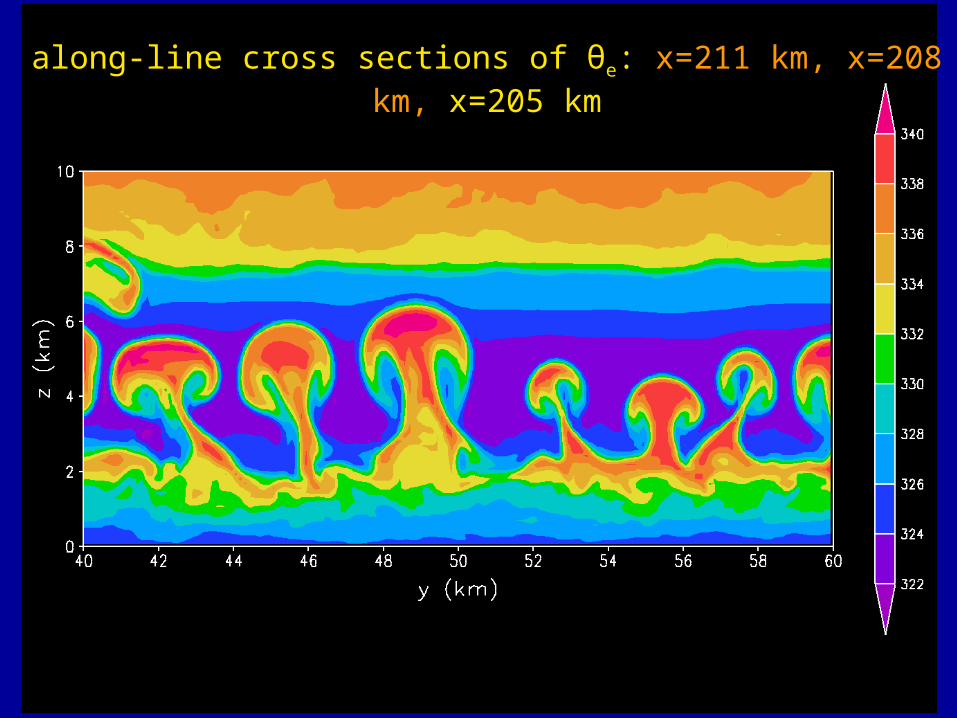
along-line cross sections of θe: x=211 km, x=208 km, x=205 km

125 m:
1000 m:
Rainwater mixing ratio
with “strong” shear

125 m:
1000 m:
θe, with “strong” shear

from: Wakimoto et al. (1996)

Perspectives on resolution
• Historical Perspective
• Theoretical Perspective
• Pragmatic Perspective

How big are convective clouds, anyway?
• Clouds are surprisingly small
• Median updraft diameters are ~2-4 km
• Updrafts of ~10 km are rare, and are usually found in supercells

Type of case Reference Measurement type Characteristic diameter (km)
Tropical oceanic Lucas et al. 1994 in situ 1.4 Š 4.1 Midlatitude continental (Thunderstorm Project)
Lucas et al. 1994 in situ 4 Š 5
Tropical oceanic Igau et al. 1999 in situ 0.5 Š 3.9 Midlatitude continental
Kyle et al. 1976 in situ 1.8 Š 4.6
Supercell Nelson 1983 Doppler radar 5 Š 15 Tropical continental Yuter and Houze
1995 Doppler radar 2 Š 4
Midlatitude continental
Musil et al. 1991 in situ 1.5 Š 15
Results of a thorough literature review
from: Bryan et al. (2006)

Some of my conclusions:
• Clouds are of O(1 km)
• Grid spacing of O(1 km) should marginally resolve convective updrafts
• I think the earliest cloud modelers knew this

The difference between resolution and grid spacing
• Grid spacing () is clear– The distance between grid cells
• Resolution is nebulous– Recall that numerical techniques cannot
properly handle features less than ~6

from: Durran (1999)
Analytic solution to the advection equation• “E” = exact• “2” = 2nd order centered• “4” = 4th-order centered

from: Durran (1999)
Analytic solution to the artificial diffusion terms• “2” = 2
• “4” = 4
• “6” = 6

Effective Resolution
• This is a relatively new concept (to some)
• The effective resolution of a numerical model is the minimum scale that is not affected by artificial aspects of the modeling system
• In the ARW Model, this is ~6-8

from: Skamarock (2004)
Kinetic energy spectra from ARW simulations

Synthesis
• O(1 km) grid spacing is needed to resolve nonhydrostatic processes
• Deep convective clouds are of O(1 km), and some supercells are of O(10 km)
• The ARW Model needs ~6-8 to “resolve” a feature
1 km grid spacing is looking marginal

Scales in turbulent flows
• L is the scale of the large eddies– e.g., a Cu cloud
is the scale of the dissipative eddies– e.g., the cauliflower-like “puffiness”


Turbulence
• Small-scale turbulence cannot be resolved in numerical models
• Theory is clear (Kolmogorov 1940)
• To resolve all scales in clouds requires ~0.1 mm grid spacing (Corrsin 1961)
• So, what should we do … ?

The filtered Navier-Stokes equations
ui
t
uiu j
x j
1
p
xi
2ui
xix j
Start with:
Apply a filter, rearrange terms
uir
t
uiru j
r
x j
1
pr
xi
2ui
r
xix j
ij
x j
All sub-filter-scale flow is contained in the term (the subgrid turbulent flux)
from Bryan et al. (2003)

Modeling subgrid turbulence
• We have a fairly good idea of how to parameterize for many flows
• HOWEVER … a few rules apply

Scales in turbulent flows
• L is the scale of the large eddies– e.g., a Cu cloud
is the scale of the dissipative eddies– e.g., the cauliflower-like “puffiness”

E(κ)
κ
Turbulence Kinetic Energy SpectrumTurbulence Kinetic Energy Spectrum
1/L 1/η
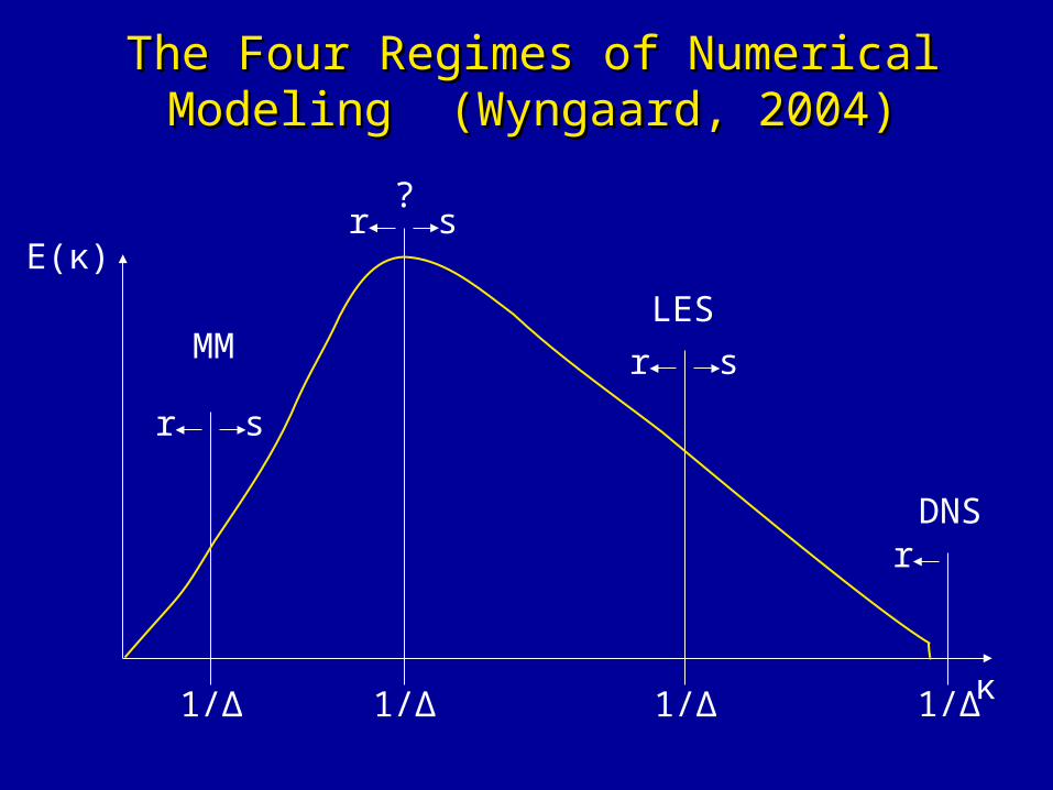
The Four Regimes of Numerical Modeling The Four Regimes of Numerical Modeling (Wyngaard, 2004)(Wyngaard, 2004)
sr
1/Δ
MM sr
1/Δ
LES
r
1/Δ
DNS
sr
1/Δ
?
E(κ)
κ

Mean flow
kinetic energy
Turbulent kinetic energy (large eddies)
Internal energy of
fluid (heat)
Corrsin (1960)
“Crude representation of average energy degradation path”
Turbulent kinetic energy (small eddies)
(A Roadmap!)

Mean flow
kinetic energy
Turbulent kinetic energy (large eddies)
Roadmap for LES

Mean flow
kinetic energy
Turbulent kinetic energy (large eddies)
Roadmap for LES
Transfer of kinetic energy to unresolved scales

LES subgrid model
• Works well if grid spacing () is 10-100 times smaller than the large eddies (L)
• Recall: L~2-4 km– Suggests that needs to be ~20-200 m
• If we want to use LES models … and we do … then of O(100 m) might be necessary

Early cloud modelers knew this
• Klemp and Wilhelmson (1978):– “. . . closure techniques for the subgrid
equations are based on the existence of a grid scale within the inertial subrange and with present resolution [Δx = 1 km] this requirement is not satisfied.”

Mean flow
kinetic energy
Turbulent kinetic energy (large eddies)
A problem: we want to do this ….
Transfer of kinetic energy to unresolved scales

Mean flow
kinetic energy
Turbulent kinetic energy (large eddies)
… but we’re really doing this with 1-4 km grid spacing
Removal of kinetic energy

Summary of theoretical section
• There is compelling evidence to use grid spacing less than 1 km– if you are interested in cloud-scale
processes
• There is very little evidence in support of grid spacing of ~4 km– unless you are only looking at the
mesoscale processes

Perspectives on resolution
• Historical Perspective
• Theoretical Perspective
• Pragmatic Perspective

Technical aspects
• Obviously, 100 m grid spacing is not accessible to all problems– It requires a great deal of RAM– It takes a long time to run– It generates an obscene amount of output
• We do real-time simulations with 4 km grid spacing because we can– Results are better than using a convective
parameterization

A new question:
• Given that:– many application are forced to use grid
spacing of 1-4 km …– grid spacing of ~100 m seems to be the
“ideal” choice …
• Then:– what are the implications of using 1-4 km
grid spacing?

The answer …
• … is coming from a new set of simulations
• Designed carefully, considering:– Numerical techniques– Effective resolution– Bridging the studies by Weisman et al. (1997)
and Bryan et al. (2003)
• Uses Bryan-Fritsch Model (much like ARW)

Overview of Simulations
periodic
periodic
openopen
Domain: 512 km x 128 km x 18 km
Cold pool
• Depth = 2.5 km
• Min. surface = -6 K

Initial Conditions: horizontally homogeneous
CAPE 2700 J/kg: slightly more unstable than Weisman et al. (1997)
Weak shear confined to lowest 2.5 km

Design of simulations (cont.)• Parameterizations:
– Ice microphysics (Lin et al., 1983)– No radiation– No surface fluxes– Subgrid turbulence (TKE, Deardorff 1980)
• Grid spacing:– Δx = 8, 4, 2, 1, 0.5, 0.25, 0.125 km– Δz = 0.25 km
(except: Δz = 0.125 km for Δx = 0.125 km)

System structure:
Composite reflectivity (dBZ) at t = 5 h
NOTE: better representation of stratiform region

System structure:
Line-averaged reflectivity (dBZ) and cloud boundary (white contour) at t = 5 h
NOTE: high cloud tops ( > 14 km )
NOTE: better representation of stratiform region

Results: Maximum w (m/s)
Higher resolution

Domain-total upward mass flux (1011 kg/s)
Higher resolution

Summary of early development
• Compared to higher resolution simulations:– With = 4 km, development is too slow– With = 4 km, systems become too intense
• For the higher resolution simulations:– Possible convergence for < 0.25 km– Remember: we are looking for a resolution-
independent result

System structure:
Composite reflectivity (dBZ) at t = 5 h

Accumulated precipitation (cm)
(t = 3 - 5 h)

Domain-total accumulated rainfall (t = 3 - 5 h)

Summary of system structure
• With < 1 km:– Squall line has better stratiform region– Simulations produce less rainfall
• Thus, inadequate resolution may explain the biases we see in real-time forecasts using ARW with 4 km grid spacing

Vertical velocity (w) at z = 5 km, t = 5 h

Vertical velocity (w) at z = 5 km, t = 5 h

Vertical velocity (w) at z = 5 km, t = 5 h

Vertical velocity spectra, z = 5 km, t = 3-5 h
Thick solid: scales above 6 Thin dashed: scales below 6

Vertical velocity spectra, z = 5 km, t = 3-5 h
L = 24 kmfor x = 4 km
L = 4 kmfor x = 0.5, 0.25 km
Thick solid: scales above 6 Thin dashed: scales below 6

Summary of updraft properties
• Updrafts are poorly resolved when 1 km– Updraft size scales with the model’s diffusive
cutoff– Updraft spacing and size keeps changing as
changes
• Updraft properties converge when 500 m– Updraft spacing is ~4 km– Updraft width is ~2 km

Summary
Horizontal grid spacing, :
10 km 1 km 0.1 km
Representation of nonhydrostatic processes:
Representation of turbulent processes:

Summary
Horizontal grid spacing, :
10 km 1 km 0.1 km
Representation of nonhydrostatic processes:
Poor
Representation of turbulent processes:
Poor

Summary
Horizontal grid spacing, :
10 km 1 km 0.1 km
Representation of nonhydrostatic processes:
Poor Ok
Representation of turbulent processes:
Poor Poor

Summary
Horizontal grid spacing, :
10 km 1 km 0.1 km
Representation of nonhydrostatic processes:
Poor Ok Good
Representation of turbulent processes:
Poor Poor Ok / Good

Summary• There are probably systematic biases in
simulations that use 1-4 km grid spacing
• Convection initiation is too slow– Updrafts are too wide– Mass flux will be too large
• Convection is too intense– Strong shear environment might be better
• This might explain some errors in real-time, 4-km simulations over central USA

1 km vs. 100 m
1 km grid spacing:
• Accurately reproduces mesoscale dynamics
• Provides useful forecast guidance
• More appropriate for high shear cases
100 m grid spacing:
Theoretically more appropriate given current understanding turbulence (terra incognita)
Required for studies of cloud-scale processes (e.g., entrainment)

My advice
• Grid spacing that you use must be a compromise between:– What is tractable– What is really needed
• 1-4 km grid spacing is good for overall system structure, propagation
• ~100 m should be desired when no observations are available

<end of Part II>


