81
SPECIAL COURSE IN MATHEMATICS SHARIPOV R. A. REPRESENTATIONS OF FINITE GROUPS Part 1 Ufa 1995
| Date post: | 18-Dec-2016 |
| Category: |
Documents |
| Upload: | ruslan-sharipov |
| View: | 212 times |
| Download: | 0 times |

arX
iv:m
ath/
0612
104v
1 [
mat
h.H
O]
4 D
ec 2
006
SPECIAL COURSE IN MATHEMATICS
SHARIPOV R.A.
REPRESENTATIONS OF FINITE GROUPS
Part 1
Ufa 1995

2
UDC 517.9Sharipov R. A. Representations of finite groups. Part 1.
The textbook — Ufa, 1995. — 75 pages — ISBN 5-87855-004-0.
This book is an introduction to a fast developing branchof mathematics — the theory of representations of groups. Itpresents classical results of this theory concerning finite groups.This book is written on the base of the special course which Igave in Mathematics Department of Bashkir State University.
In preparing Russian edition of this book I used computertypesetting on the base of AMS-TEX package and I used cyrillicfonts of Lh-family distributed by CyrTUG association of CyrillicTEX users. English edition is also typeset by AMS-TEX.
ISBN 5-87855-004-0 c© Sharipov R.A., 1995English Translation c© Sharipov R.A., 2006

3
CONTENTS.
CONTENTS. ...................................................................... 3.
PREFACE. ......................................................................... 4.
CHAPTER I. REPRESENTATIONS OF GROUPS. ............. 5.
§ 1. Representations of groups and their homomorphisms. ..... 5.§ 2. Finite dimensional representations. ................................ 7.§ 3. Invariant subspaces. Restriction and factorization
of representations. ........................................................ 8.§ 4. Completely reducible representations. .......................... 11.§ 5. Schur’s lemma and some corollaries of it. ..................... 21.§ 6. Irreducible representations of the direct product
of groups. .................................................................. 27.§ 7. Unitary representations. .............................................. 36.
CHAPTER II. REPRESENTATIONS OF FINITEGROUPS. ................................................................ 44.
§ 1. Regular representations of finite groups. ....................... 44.§ 2. Invariant averaging over a finite group. ........................ 46.§ 3. Characters of group representations. ........................... 50.§ 4. Orthogonality relationships. ........................................ 54.§ 5. Expansion into irreducible components. ........................ 65.
CONTACTS. ................................................................... 75.
APPENDIX. ................................................................... 76.

PREFACE.
The theory of group representations is a wide branch of math-ematics. In this book I explain very small part of this theoryconcerned with representations of finite groups. The material ofthe book is approximately equal to a one semester course.
In explaining the material of the book I tried to make itmaximally detailed, complete and self-consistent. The readerneed not refer to other literature. He is only required to knowthe linear algebra and the group theory on the level of a standarduniversity course. The linear algebra references are given to mybook which now is available online:
[1] Sharipov R. A. «Course of linear algebra and multidimen-sional geometry», Bashkir State University, Ufa 1996.
The primary material of the book is prepared on the base of thefollowing two brilliant monographs:
[2] Neimark M. A. «Theory of representations of groups», Naukapublishers, Moscow 1976;
[3] Kirillov A. A. «Elements of the theory of representations»,Nauka publishers, Moscow 1978.
Some problems concerning the character algebra for finitegroups representations are not considered in this book. They willbe given in Part 2, which is planned as a separate book.
September, 1995;December, 2006. R. A. Sharipov.

CHAPTER I
REPRESENTATIONS OF GROUPS
§ 1. Representations of groups
and their homomorphisms.
It is clear that matrix groups are in some sense simpler thanabstract groups. Multiplication rule in them is explicitly specific.Dealing with matrix groups one can use methods of the linearalgebra and calculus. The theory of group representations growsfrom the aim to reproduce an abstract group in a matrix form.
Let V be a linear vector space over the field of complexnumbers C. By End(V ) we denote the set of linear operatorsmapping V into V . The subset of non-degenerate operatorswithin End(V ) is denoted by Aut(V ). It is easy to see thatAut(V ) is a group. The operation of composition, i. e. applyingtwo operators successively, is the group multiplication in Aut(V ).
Definition 1.1. A representation f of a group G in a linearvector space V is a group homomorphism f : G→ Aut(V ).
If f is a representation of a group G in V , this fact is brieflywritten as (f,G, V ). Let g ∈ G be an element of the groupG , then f(g) is a non-degenerate operator acting within thespace V . It is called the representation operator correspondingto the element g ∈ G. By f(g)x we denote the result of applyingthis operator to a vector x ∈ V . The notation with two pairsof braces f(g)(x) will also be used provided it is more clear

6 CHAPTER I. REPRESENTATIONS OF GROUPS.
in a given context. For instance, f(g)(x + y). Representationoperators satisfy the following evident relationships:
(1) f(g1 g2) = f(g1) f(g2);(2) f(1) = 1;(3) f(g−1) = f(g)−1;
Definition 1.2. Let (f,G, V ) and (h,G,W ) be two represen-tations of the same group G. A linear mapping A : V → W iscalled a homomorphism sending the representation (f,G, V ) tothe representation (h,G,W ) if the following condition is fulfilled:
A ◦ f(g) = h(g) ◦A for all g ∈ G. (1.1)
The mapping A in (1.1), which performs a homomorphism of tworepresentations, sometimes is called an interlacing map.
Definition 1.3. A homomorphism A interlacing two repre-sentations (f,G, V ) and (h,G,W ) is called an isomorphism if itis bijective as a linear mapping A : V →W .
It is easy to verify that the relation of being isomorphic is anequivalence relation for representations. Two isomorphic repre-sentations are also called equivalent representations. In the theoryof representations two isomorphic representations are treated asidentical representations because all essential properties of suchtwo representations do coincide.
Theorem 1.1. If (f,G, V ) is a representation of a group G ina space V and if A : V → W is a bijective linear mapping, thenA induces a unique representation of the group G in W which isequivalent to (f,G, V ) and for which A is an interlacing map.
Proof. The proof of the theorem is trivial. Let’s define theoperators of a representation h in W as follows:
h(g) = A ◦ f(g) ◦A−1. (1.2)
It is easy to verify that the formula (1.2) does actually definea representation of the group G in W . Multiplying (1.2) on

§ 2. FINITE-DIMENSIONAL REPRESENTATIONS. 7
the right by A, we get (1.1). Hence A is an isomorphism of fand h. Moreover, any representation of G in W for which A isan interlacing isomorphism should coincide with h. This fact isproved by multiplying (1.1) on the right by A−1. �
From the theorem proved just above we conclude that if arepresentation f in V is given, in order to construct an equivalentrepresentation in W it is sufficient to have a linear bijection fromV to W . However, in practice the problem is stated somewhatdifferently. Two representations f and h in V and W are alreadygiven. The problem is to figure out if they are equivalent and ifso to find an interlacing operator. In this statement this is one ofthe basic problems of the theory of representations.
§ 2. Finite dimensional representations.
Definition 2.1. A representation (f,G, V ) is called finite-dimensional if its space V is a finite-dimensional linear vectorspace, i. e. dimV <∞.
Below in this book we consider only finite-dimensional rep-resentations, though many facts proved for this case can thenbe transferred or generalized for the case of infinite-dimensionalrepresentations.
Note that any finite-dimensional linear vector space over thefield of complex numbers C can be bijectively mapped ontothe standard arithmetic coordinate vector space Cn, wheren = dimV . And Aut(Cn) = GL(n,C). Therefore each finite-dimensional representation is equivalent to some matrix represen-tation f : G→ GL(n,C). This fact follows from the theorem 1.1.In spite of this fact we shall consider finite-dimensional represen-tations in abstract vector spaces because all statements in thiscase are more elegant and their proofs are sometimes even moresimple than the proofs of corresponding matrix statements.
CopyRight c© Sharipov R.A., 1995, 2006.

8 CHAPTER I. REPRESENTATIONS OF GROUPS.
§ 3. Invariant subspaces. Restriction
and factorization of representations.
Definition 3.1. Let (f,G, V ) be a representation of a groupG in a linear vector space V . A subspace W ⊆ V is called aninvariant subspace if for any g ∈ G and for any x ∈W the resultof applying f(g) to x belongs to W , i. e. f(g)x ∈W .
The concept of irreducibility is introduced in terms of invari-ant subspaces. This is the central concept in the theory ofrepresentations.
Definition 3.2. A representation (f,G, V ) of the group Gis called irreducible if it has no invariant subspaces other thanW = {0} and W = V . Otherwise the representation (f,G, V ) iscalled reducible.
Assume that (f,G, V ) is an irreducible representation. Let’schoose some vector x 6= 0 of V and consider its orbit:
Orbf (x) = {y ∈ V : y = f(g)x for some g ∈ G }.
The orbit Orbf (x) is a subset of the space V invariant under theaction of the representation operators. However, in general case,it is not a linear subspace. Let’s consider its linear span
W = 〈Orbf (x)〉.
The subspace W is invariant and W 6= {0} since it possesses thenon-zero vector x. Then due to the irreducibility of f we getW = V . As a result one can formulate the following criterion ofirreducibility.
Theorem 3.1 (irreducibility criterion). A representation(f,G, V ) is irreducible if and only if the orbit of an arbitrary non-zero vector x ∈ V spans the whole space V .
The necessity of this condition was proved above. Let’s proveits sufficiency. Let W ⊆ V be an invariant subspace such that

§ 3. INVARIANT SUBSPACES. 9
W 6= {0}. Let’s choose a nonzero vector x ∈ W . Due to theinvariance of W we have Orbf (x) ⊆ W . Hence, 〈Orbf (x)〉 ⊆ W .But 〈Orbf (x)〉 = V , therefore W = V . The criterion is proved.
Irreducible representations are similar to chemical elements.One cannot extract other more simple representations of a givengroup from them. Any reducible representation in some sensesplits into irreducible ones. Therefore in the theory of represen-tations the following two problems are solved:
(1) to find and describe all irreducible representations of a givengroup;
(2) to suggest a method for splitting an arbitrary representationinto its irreducible components.
The first problem is analogous to building the Mendeleev’s ta-ble in chemistry, the second problem is analogous to chemicalanalysis of substances.
Let’s consider some reducible representation (f,G, V ) of agroup G. Assume that W is an invariant subspace such that{0} ( W ( V . Let’s denote by ϕ(g) the restriction of theoperator f(g) to the subspace W :
ϕ(g) = f(g)W
. (3.1)
For the operators ϕ(g) we have the following relationships:
ϕ(g)ϕ(g−1) = (f(g) f(g−1))W
= 1; (3.2)
ϕ(g1)ϕ(g2) = (f(g1) f(g2))W
= ϕ(g1 g2). (3.3)
From the relationship (3.2) we conclude that the operator ϕ(g)is invertible and ϕ(g)−1 = ϕ(g−1). Hence, ϕ(g) ∈ Aut(W ).The relationship (3.3) in its turn shows that the mappingϕ : G → Aut(W ) is a group homomorphism defining a repre-sentation.

10 CHAPTER I. REPRESENTATIONS OF GROUPS.
Definition 3.3. The representation (ϕ,G,W ) of a group Gobtained by restricting the operators of a representation (f,G, V )to its invariant subspace W ⊆ V according to the formula (3.1)is called the restriction of f to W .
The presence of an invariant subspace W let’s us define fac-toroperators in the factorspace V/W :
ψ(g) = f(g)V/W
. (3.4)
Let’s recall that the action of the operator ψ(g) upon a cosetClW (x) in V/W is defined as follows:
ψ(g)ClW (x) = ClW (f(g)x). (3.5)
The correctness of the definition (3.5) is verified by direct cal-culations (see [1]). The factoroperators (3.5) obey the followingrelationships:
ψ(g)ψ(g−1)ClW (x) = ClW (f(g)f(g−1)x) =
= ClW (f(g g−1)x) = ClW (x),(3.6)
ψ(g1)ψ(g2)ClW (x) = ClW (f(g1)f(g2)x) =
= ClW (f(g1 g2)x) = ψ(g1 g2)ClW (x).(3.7)
From (3.6) and (3.7) we conclude that the factoroperators (3.4)satisfy the relationships similar to (3.2) and (3.3). They define arepresentation (ψ,G, V/W ) which is usually called a factorrepre-
sentation.The representations (ϕ,G,W ) and (ψ,G, V/W ) are generated
by the representation f . Each of them inherits a part of theinformation contained in the representation f . In order tounderstand which part of the information is kept in ϕ and ψ let’sstudy the representation operators f(g) in some special basis.Let’s choose a basis e1, . . . , es within the invariant subspace W .
§ 4. COMPLETELY REDUCIBLE REPRESENTATIONS. 11
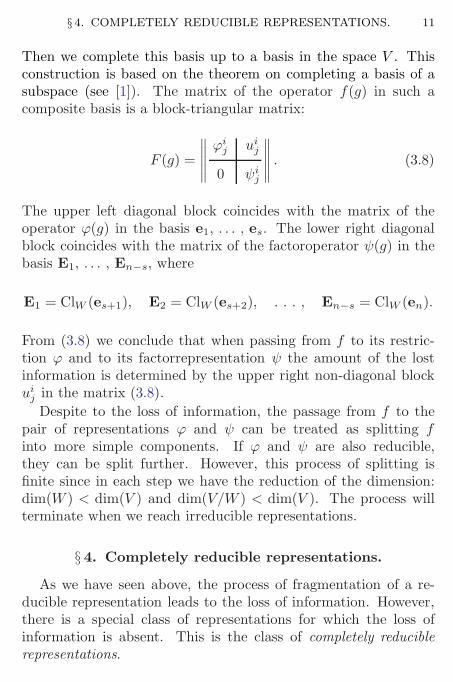
Then we complete this basis up to a basis in the space V . Thisconstruction is based on the theorem on completing a basis of asubspace (see [1]). The matrix of the operator f(g) in such acomposite basis is a block-triangular matrix:
F (g) =
∥
∥
∥
∥
∥
ϕij ui
j
0 ψij
∥
∥
∥
∥
∥
. (3.8)
The upper left diagonal block coincides with the matrix of theoperator ϕ(g) in the basis e1, . . . , es. The lower right diagonalblock coincides with the matrix of the factoroperator ψ(g) in thebasis E1, . . . , En−s, where
E1 = ClW (es+1), E2 = ClW (es+2), . . . , En−s = ClW (en).
From (3.8) we conclude that when passing from f to its restric-tion ϕ and to its factorrepresentation ψ the amount of the lostinformation is determined by the upper right non-diagonal blockui
j in the matrix (3.8).
Despite to the loss of information, the passage from f to thepair of representations ϕ and ψ can be treated as splitting finto more simple components. If ϕ and ψ are also reducible,they can be split further. However, this process of splitting isfinite since in each step we have the reduction of the dimension:dim(W ) < dim(V ) and dim(V/W ) < dim(V ). The process willterminate when we reach irreducible representations.
§ 4. Completely reducible representations.
As we have seen above, the process of fragmentation of a re-ducible representation leads to the loss of information. However,there is a special class of representations for which the loss ofinformation is absent. This is the class of completely reducible
representations.

12 CHAPTER I. REPRESENTATIONS OF GROUPS.
Definition 4.1. A representation (f,G, V ) of a group G iscalled completely reducible if each its invariant subspace W hasan invariant direct complement U , i. e. V is a direct sum of twoinvariant subspaces V = W ⊕ U .
Note that an irreducible representation is a trivial example ofa completely reducible one. Here wee have V = V ⊕ {0}.
Let (f,G, V ) be a reducible and completely reducible repre-sentation. Let W be an invariant subspace for f and U beits invariant direct complement. Then we have the followingisomorphisms of the restrictions and factors:
fU
∼= fV/W
, fW
∼= fV/U
. (4.1)
In order to prove (4.1) lets consider again a basis e1, . . . , es in Uand complement it with a basis h1, . . . , hn−s in U . Let’s denotees+1 = h1, . . . , en = hn−s. As a result of such a reunion ofbases we get a basis in V . Let’s define a mapping A : U → V/Wby setting
Ax = ClW (x) for all x ∈ U. (4.2)
From (4.2) one easily derives the values of the mapping A onbasis vectors
A(h1) = E1, . . . , A(hn−s) = En−s. (4.3)
The mapping A establishes bijective correspondence of bases ofU and V/W . For this reason it is bijective. Let’s verify thatit implements an isomorphism of representations, i. e. let’s verifythe relationship (1.1) for A:
A(f(g)hi) = ClW (f(g)hi) = ψ(g)ClW (hi) = ψ(g)A(hi).
This relationship proves the first isomorphism in (4.1). It isimplemented by the mapping A defined in (4.2).
§ 4. COMPLETELY REDUCIBLE REPRESENTATIONS. 13
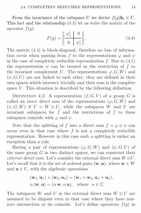
From the invariance of the subspace U we derive f(g)hi ∈ U .This fact and the relationship (4.3) let us write the matrix of theoperator f(g):
F (g) =
∥
∥
∥
∥
∥
ϕij 0
0 ψij
∥
∥
∥
∥
∥
. (4.4)
The matrix (4.4) is block-diagonal, therefore no loss of informa-tion occur when passing from f to the representations ϕ and ψin the case of completely reducible representation f . Due to (4.1)the representation ψ can be treated as the restriction of f tothe invariant complement U . The representations ϕ,G,W ) and(ψ,G,U) are not linked to each other, they are defined in theirown spaces which intersect trivially and their sum is the completespace V . This situation is described by the following definition.
Definition 4.2. A representation (f,G, V ) of a group G iscalled an inner direct sum of the representations (ϕ,G,W ) and(ψ,G,W ) if V = W ⊕ U , while the subspaces W and U areinvariant subspaces for f and the restrictions of f to thesesubspaces coincide with ϕ and ψ.
Note that the splitting of f into a direct sum f = ϕ ⊕ ψ canoccur even in that case where f is not a completely reduciblerepresentation. However in this case such a splitting is rather anexception than a rule.
Having a pair of representations (ϕ,G,W ) and (ψ,G,U) ofthe same group G in two distinct spaces, we can construct theirexterior direct sum. Let’s consider the external direct sum W⊕U .Let’s recall that it is the set of ordered pairs (w,u), where w ∈Wand u ∈ U , with the algebraic operations
(w1,u1) + (w2,u2) = (w1 + w2,u1 + u2),
α (w,u) = (αw, αu), where α ∈ C.
The subspaces W and U in the external direct sum W ⊕ U areassumed to be disjoint even in that case where they have non-zero intersection or do coincide. Let’s define operators f(g) in
14 CHAPTER I. REPRESENTATIONS OF GROUPS.
W ⊕ U as follows:
f(g)(w,u) = (ϕ(g)w, ψ(g)u). (4.5)
The representation (f,G,W ⊕ U) constructed according to therepresentation (4.5) is called the external direct sum of the repre-sentations (ϕ,G,W ) and (ψ,G,W ). It is denoted f = ϕ⊕ψ. Thedifference of internal and external direct sums is rather formal,their properties do coincide in most.
Assume that the space V of a representation (f,G, V ) isexpanded into a direct sum of subspaces V = W ⊕ U (notnecessarily invariant ones). Each such an expansion are uniquelyassociated with two projection operators P and Q. The projectorP is the projection operator that projects onto the subspace Wparallel to the subspace U , while Q projects onto U parallel toW . They satisfy the following relationships:
P 2 = P, Q2 = Q, P +Q = 1. (4.6)
Moreover, W = ImP and U = ImQ. These properties of theprojection operators are well known (see [1]).
Lemma 4.1. The subspace W in an expansion V = W ⊕ U isinvariant with respect to the operators of a representation f,G, V )if and only if the corresponding projector P obeys the relationship
(P ◦ f(g) − f(g) ◦P ) ◦P = 0 for all g ∈ G. (4.7)
The invariance of both subspaces W and U in an expansion V =W ⊕ U is equivalent to the relationship
(P ◦ f(g) = f(g) ◦P ) for all g ∈ G, (4.8)
which means that the projector P commutes with all operators ofthe representation f .
CopyRight c© Sharipov R.A., 1995, 2006.

§ 4. COMPLETELY REDUCIBLE REPRESENTATIONS. 15
Let x be an arbitrary vector. Then Px ∈ W . In the case ofan invariant subspace W the vector y = f(g)Px also belongs toW . For the vector y ∈W we have Py = y. Therefore
Pf(g)Px = f(g)Px = f(g)P 2x. (4.9)
Comparing the left and right hand sides of the equality (4.9) andtaking into account the arbitrariness of the vector x, we easilyderive the relationship (4.7) in the statement of the lemma.
And conversely, from the relationship (4.7), using the propertyP 2 = P from (4.6), we easily derive (4.9). From (4.9) we derivethat the vector f(g)Px belongs to W for an arbitrary vector x.Let’s choose x ∈W and from Px = x for such a vector x we findthat f(g)x belongs to W . The invariance of W is established. Inorder to prove the second statement of the lemma let’s write therelationship (4.7) for the projector Q:
(Q ◦ f(g) − f(g) ◦Q) ◦Q = 0. (4.10)
from Q = 1 − P we get Q ◦ f(g) − f(g) ◦Q = f(g) ◦P − P ◦ f(g).Therefore the relationship (4.10) is rewritten as
f(g) ◦P − P ◦ f(g) + (P ◦ f(g) − f(g) ◦P ) ◦P = 0.
Then, taking into account (4.7), we reduce it to the relationship(4.8), which means that the operators P and f(g) do commute.The lemma is proved.
The second proposition of the lemma 4.1 can be generalizedfor the case where V is expanded into a direct sum of severalsubspaces. Assume that V = W1 ⊕ . . . ⊕ Ws. Let’s recall(see [1]) that this expansion uniquely fixes a concordant familyof projection operators P1, . . . , Ps. They obey the followingconcordance relationships:
(Pi)2 = Pi, P1 + . . . + Ps = 1,
Pi ◦Pj = 0 for i 6= j, Pi ◦Pj = Pj ◦Pi.

16 CHAPTER I. REPRESENTATIONS OF GROUPS.
Moreover, Wi = ImPi. The condition of invariance of all sub-spaces Wi in the expansion V = W1 ⊕ . . . ⊕ Ws with respectto representation operators of a representation (f,G, V ) in termsof the corresponding projection operators is formulated in thefollowing lemma. We leave its proof to the reader.
Lemma 4.2. The expansion V = W1⊕. . .⊕Ws is an expansionof V into a direct sum of invariant subspaces of the representation(f,G, V ) if and only if all projection operators Pi associated withthe expansion V = W1⊕. . .⊕Ws commute with the representationoperators f(g).
Let’s consider a completely reducible finite-dimensional rep-resentation (f,G, V ) split into a direct sum of its restrictionsto invariant subspaces f = ϕ ⊕ ψ. Assume that the restrictionϕ of f to the subspace W is reducible and assume that W1 isits non-trivial invariant subspace: {0} ( W1 ( W . Then thesubspace W1 is invariant with respect to f . It has an invariantcomplement U1. Let’s consider the expansions
V = W ⊕ U, V = W1 ⊕ U1. (4.11)
Note that W1 ⊂ W , hence, W + U1 = V . Therefore the dimen-sions of the subspaces in (4.11) are related as follows:
dim(W ) + dim(U1) − dim(V ) = dim(W ) − dim(W1) > 0.
From this relationship, we see that the intersection W2 = W ∩U1
is non-zero and its dimension is given by the formula
dim(W ∩ U1) = dim(W ) − dim(W1). (4.12)
Now note that W1 ∩W2 = {0} since W2 ⊂ U1. Therefore, due to(4.12) the subspace W is expanded into the direct sum
W = W1 ⊕W2,

§ 4. COMPLETELY REDUCIBLE REPRESENTATIONS. 17
each summand in which is invariant with respect to f and, hence,with respect to ϕ. Thus, we have proved the following importanttheorem.
Theorem 4.1. The restriction of a completely reducible finite-dimensional representation to an invariant subspace is completelyreducible.
The next theorem on the expansion into a direct sum is animmediate consequence of the theorem 4.1.
Theorem 4.2. Each finite-dimensional completely reduciblerepresentation f is expanded into a direct sum of irreducible rep-resentations
f = f1 ⊕ . . .⊕ fk, V = W1 ⊕ . . .⊕Wk, (4.13)
where each fi is a restriction of f to the corresponding invariantsubspace Wi.
Note that in general the expansion (4.13) is not unique. Let’sconsider two expansions of f into irreducible components:
f = f1 ⊕ . . .⊕ fk, V = W1 ⊕ . . .⊕Wk,(4.14)
f = f1 ⊕ . . .⊕ fk, V = W1 ⊕ . . .⊕ Wk.
The extent of differences in two expansions (4.14) is determinedby the following Jordan-Holder theorem.
Theorem 4.3. The numbers of irreducible components in theexpansions (4.14) are the same: q = k, and there is a transposition
σ ∈ Sk such that (fi, G,Wi) ∼= (fσi, G, Wσi).
The expansions (4.14) are isomorphic up to a transpositionof components. However, we should emphasize that the isomor-phism does not mean the coincidence of these expansions.
We shall prove the Jordan-Holder theorem by induction on thenumber of components k in the first expansion (4.14).

18 CHAPTER I. REPRESENTATIONS OF GROUPS.
The base of the induction: k = 1, V = W1. In this casethe representation f = f1 is irreducible. Therefore q = 1 = k andW1 = V , f1 = f = f1. The base of the induction is proved.
The inductive step. Assume that the theorem is valid forrepresentations possessing at least one expansion of the form(4.13) with the length k − 1. For the representation f weintroduce the following notations:
Vi = W1 ⊕ . . .⊕ Wi where i = 1, . . . , q,
U = W1 ⊕ . . .⊕Wk−1 and Ui = Vi ∩ U.(4.15)
All of the subspaces in (4.15) are invariant with respect to f .Moreover, V = U ⊕Wk and there are two chains of inclusions:
{0} ( V1 ( . . . ( Vq = V,
{0} ( U1 ( . . . ( Uq = U.(4.16)
Let h : V → V/U be a canonical projection onto the factorspace.Let’s denote by ϕ the factorrepresentation in the factorspace V/Uand consider the chain of invariant subspaces for it
{0} ⊆ h(V1) ⊆ . . . ⊆ h(Vq) = h(V ) = V/U ∼= Wk.
Due to the isomorphism ϕ ∼= fk we conclude that ϕ is irreducible.Hence the above chain does actually look like
{0} = h(V1) = . . . = h(Vs) ( h(Vs+1) = . . . = h(Vq) = h(V ).
Therefore Vi ⊆ U and Ui = Vi for i 6 s. For i > s + 1 we usethe isomorphisms Vi/Ui
∼= h(Vi) = h(Vi+1) ∼= Vi+1/Ui+1. But
Vi ( Vi, hence, Ui ( Ui+1. Then from (4.16) we get
{0} ( U1 ( . . . ( Us = Us+1 ( . . . ( Uq = U. (4.17)
The equality Us = Us+1 follows from the irreducibility of the
factorrepresentation ϕs+1∼= ϕ ∼= fk in the factorspace Vs+1/Vs

§ 4. COMPLETELY REDUCIBLE REPRESENTATIONS. 19
and from the inclusions Vs = Us = Us+1 ( Vs+1. Relying upon
complete reducibility of f , we choose invariant complements Wi+1
for Ui in Ui+1, i. e. Ui+1 = Ui⊕Wi+1. Then Vi+Ui+1 = Vi⊕Wi+1
is an invariant subspace in Vi+1 containing Vi and not coinciding
with it. But the factorrepresentation in Vi+1/Vi is isomorphic to
tildefi+1 and, hence, is irreducible. Therefore Vi ⊕ Wi+1 = Vi+1
and the restriction of f to Wi+1 is isomorphic to fi+1. From(4.15) and (4.17) we get
U = W1 ⊕ . . . ⊕Ws ⊕Ws+1 ⊕ . . . ⊕Wk−1,
U = W1 ⊕ . . . ⊕ Ws ⊕ Ws+2 ⊕ . . . ⊕ Wq.(4.18)
Now it is sufficient to apply the inductive hypothesis to (4.18).As a result we get k = q and find σi for i = 1, . . . , k − 1. Theisomorphism of fk and the factorrepresentation ϕs+1 in Vs+1/Vs
yields σk = s + 1 since ϕs+1∼= fs+1 by construction of the
subspaces (4.15). The Jordan-Holder theorem is proved.
Due to the theorems 4.1 and 4.2 it is natural to introduce thefollowing terminology.
Definition 4.3. An invariant subspace W ⊆ V is called anirreducible subspace for a representation (f,G, V ) if the restric-tion of f to W is irreducible.
The following theorem yields a tool for verifying the completereducibility of representations.
Theorem 4.4. A finite-dimensional representation (f,G, V )is completely reducible if and only if the set of all its irreduciblesubspaces span the whole space V .
Proof. Let {Wα}α∈A be the set of all irreducible subspacesin V . The number of such subspaces could be infinite even in thecase of a finite-dimensional representation. Let’s denote by W

20 CHAPTER I. REPRESENTATIONS OF GROUPS.
the sum of all irreducible subspaces Wα:
W =∑
α∈A
Wα =⟨
⋃
α∈A
Wα
⟩
.
The theorem 4.4 says that the condition W = V is necessaryand sufficient for the representation f to be completely reducible.The necessity of this condition follows from the theorem 4.2.Let’s prove its sufficiency. Let U = U0 be an invariant subspacefor f and {0} 6= U0 6= V . The for each irreducible subspace Wα
we have two mutually exclusive options:
Wα ⊆ U0 or Wα ∩ U0 = {0}.
And there is at least one subspace Wα1for which the second
option is valid: Wα1∩ U0 = {0}. Indeed, otherwise we would
have W ⊆ U0, which contradict W = V . Let’s consider the sum
U1 = U0 +Wα1= U0 ⊕Wα1
.
The subspace U1 is invariant with respect to f . If U1 6= V , werepeat our considerations with U1 instead of U0. As a result weget a new invariant subspace
U2 = U1 ⊕Wα2= U0 ⊕Wα1
⊕Wα2.
The process of adding new direct summand to U0 will terminateat some step since dimV <∞. As a result we get
Uk = U0 ⊕ (Wα1⊕ . . .⊕Wαk
) = V.
The the subspace W = Wα1⊕ . . . ⊕Wαk
is a required invariantdirect complement for U = U0. The theorem is proved. �

§ 5. SCHUR’S LEMMA AND SOME COROLLARIES . . . 21
§ 5. Schur’s lemma and some corollaries of it.
The theorem 4.2 proved in previous section says that eachcompletely reducible representation is expanded into a directsum of its irreducible components. In this section we study theseirreducible components by themselves. Schur’s lemma plays thecentral role in this. We formulate two versions of this lemma, thesecond version being a strengthening of the first one, but for amore special case.
Lemma 5.1 (Schur’s lemma). Let (f,G, V ) and (h,G,W )be two irreducible representations of a group G. Each homomor-phism A relating these two representations either is identicallyzero or is a homomorphism.
Before proving the Schur’s lemma we consider the followingtheorem having a separate value.
Theorem 5.1. If a linear mapping A : V → W is a homo-morphism of representations from (f,G, V ) to (h,G,W ), then itskernel KerA is an invariant subspace for f , while its image ImAis an invariant subspace for h.
Proof. Let y = AX be a vector from the image of themapping A. We apple the operator f(g) to it and use therelationship (1.1). Then we get
h(g)y = h(g)Ax = Af(g)x.
Now it is clear that h(g)y ∈ ImA, i. e. ImA is an invariantsubspace for h. The invariance of KerA is proved similarly.Assume that x ∈ KerA. Let’s apply the operator f(g) to x andthen apply the mapping A. Taking into account (1.1), we get
Af(g)x = h(g)Ax = 0
since Ax = 0. Hence, f(g)x ∈ KerA. The invariance of thekernel KerA with respect to f is proved. �
CopyRight c© Sharipov R.A., 1995, 2006.

22 CHAPTER I. REPRESENTATIONS OF GROUPS.
Now let’s proceed to proving Schur’s lemma 5.1. The case,where A = 0, is trivial. In order to exclude this case assume thatA 6= 0. Then ImA 6= {0}. According to the theorem 5.1 provedjust above, ImA is invariant with respect to the representationh. Since h is irreducible, we get ImA = W . This means that thehomomorphism A is a surjective linear mapping A : V →W .
The kernel KerA of the mapping A : V → W is invariantwith respect to f . Since f is an irreducible representation, wehave two options KerA = {0} or KerA = V . The second optionleads to the trivial case A = 0, which is excluded. Therefore,KerA = {0}. This means that A : V → W is an injective linearmapping. Being surjective and injective simultaneously, thismapping is bijective. Hence, it is an isomorphism of (f,G, V )and (h,G,W ). Schur’s lemma is proved.
Now let’s consider an operator A : V → V that interlaces anirreducible representation (f,G, V ) with itself. The relationship(1.1) written for this case means that A commute with all rep-resentation operators f(g). The second version of Schur’s lemmadescribes this special case f = g.
Lemma 5.2 (Schur’s lemma). Each operator A : V → Vthat commutes with all operators of an irreducible finite-dimen-sional representation (f,G, V ) in a linear vector space V over thefield of complex numbers C is a scalar operator, i. e. A = λ · 1,where λ ∈ C.
Proof. Let λ be an eigenvalue of the operator A and letVλ 6= {0} be the corresponding eigenspace. If x ∈ Vλ thenAx = x. Moreover, from the commutation condition of theoperators A and f(g) we obtain
Af(g)x = f(g)Ax = λf(g)x.
Hence, f(g)x is also a vector of the eigenspace Vλ. In otherwords, Vλ is an invariant subspace. Since Vλ 6= {0} and since fis irreducible, we get Vλ = V . Hence, Ax = x for an arbitraryvector x ∈ V . This means that A = λ · 1. �

§ 5. SCHUR’S LEMMA AND SOME COROLLARIES . . . 23
Note that the condition of finite-dimensionality of the repre-sentation f and the condition of complexity of the vector spaceV in Schur’s lemma 5.2 are essential. Without these conditionsone cannot grant the existence of a non-trivial eigenspace.
Now we apply Schur’s lemma for to investigate tensor productsof representations of some special sort. For this reason we needto define the concept of tensor product for representations.
Let (f, g, V ) and (h,G,W ) be two representations of a groupG. We define the operators ϕ(g) acting within the tensor productV ⊗W by setting
ϕ(g)(v ⊗ w) = (f(g)v ⊗ h(g)w) for all g ∈ G. (5.1)
The operators ϕ(g) constitute a new representation of the groupG. The proof of this proposition and verifying the correctness ofthe formula (5.1) are left to the reader.
Definition 5.1. The representation (ϕ,G, V ⊗W ) given bythe operators (5.1) is called the tensor product of the representa-tions f and h. It is denoted ϕ = f ⊗ h.
Note that the construction (5.1) is easily generalized for thecase of several representations.
Assume that the representation f in the construction (5.1)is irreducible. As a second tensorial multiplicand in (5.1) wechoose the trivial representation i given by the identity operatorsi(g) = 1 for all g ∈ G. In the case where dimW > 1 the tensorproduct f ⊗ i is a reducible representation. Let’s prove this fact.Assume that e1, . . . , em is a basis in the space W . Let’s denoteby Wk one-dimensional subspaces spanned by basis vectors ek
and then consider the subspaces
V ⊗Wk, k = 1, . . . , m. (5.2)
The subspaces (5.2) are invariant within V ⊗ W with respectto the operators of the representation f ⊗ i.The restrictions off ⊗ i to V ⊗Wk all are isomorphic to f . Hence, the subspaces

24 CHAPTER I. REPRESENTATIONS OF GROUPS.
(5.2) are irreducible. These results are simple. They are provedimmediately.
No note that V ⊗W = V ⊗W1 ⊕ . . . ⊕ V ⊗Wm. The spaceV ⊗W is a sum of its irreducible subspaces V ⊗Wk. Hence itis spanned by these subspaces. Therefore, it is sufficient to applythe theorem 4.4. As a result we get the following proposition.
Theorem 5.2. The tensor product f⊗i of a finite-dimensionalirreducible representation f and a trivial finite-dimensional rep-resentation i is completely reducible.
By means of this theorem one can describe the structure of allinvariant subspaces of the tensor product f ⊗ i.
Theorem 5.3. If under the assumptions of the theorem 5.2 fand i are representations in complex linear vector spaces V andW , then each invariant subspace of the representation f ⊗ i is atensor product U = V ⊗ W , where W is some subspace of W .
Proof. Let U be some invariant subspace of f ⊗ i in V ⊗W .Due to the theorem 5.2 the representation f ⊗ i is completelyreducible. Therefore U has an invariant complement U . Theexpansion V ×W = U ⊕ U means that we can define a projectionoperator P that project onto U parallel to U . The invariance ofboth spaces U and U means that P commutes with all operatorsof the representation ϕ = f × i.
Let A : V × W → V × W be some operator in the tensorproduct V ×W . In our proof A = P , however, we return to thisspecial case a little bit later. Let’s apply the operator A to x⊗ej
and write the result as
A(x ⊗ ej) =
m∑
j=1
Akj (x) ⊗ ek. (5.3)
Here e1, . . . , em is some basis in W . Since basis vectors arelinearly independent, the coefficients Ak
j (x) ∈ V in the expansion(5.3) are unique. They are changed only if we change a basis,

§ 5. SCHUR’S LEMMA AND SOME COROLLARIES . . . 25
the transformation rule for them being analogous to that forcomponents of a tensor. This fact is not important for us, sincein our considerations we will not change the basis e1, . . . , em.
Let’s study the dependence of Akj (x) on x. It is clear that it is
linear. Therefore each coefficient Akj (x) in (5.3) defines a linear
operator Akj : V → V . Let’s write the commutation relationship
for A and ϕ(g). It is sufficient write this relationship as appliedto the vectors of the form x⊗ ei. From (5.3) we derive
A ◦ϕ(g)(x ⊗ ei) =
m∑
k=1
Akj
◦ f(g)(x) ⊗ ek,
ϕ(g) ◦A(x ⊗ ei) =
m∑
k=1
f(g) ◦Akj (x) ⊗ ek.
(5.4)
For to write (5.4) it is sufficient to recall that ϕ = f ⊗ i, where iis a trivial representation. From (5.4), it is easy to see that thecommutation relationship A ◦ϕ(g) = ϕ(g) ◦A is equivalent to
f(g) ◦Akj = Ak
j ◦ f(g). (5.5)
Thus, all of the linear operators Akj commute with the operators
f(g) of the representation f .The next step in proof is to return to the projection operator
A = P (see above) and to apply Schur’s lemma to the operatorsAk
j = P kj . The projector P commutes with ϕ(g), therefore
the relationships (5.5) hold for Akj = P k
j . Applying Schur’slemma 5.2, we get
P kj = λk
j × 1, (5.6)
where λkj are some complex numbers. Substituting (5.6) into the
expansion (5.3), for the operator P we derive:
P (x ⊗ ej) =m∑
k=1
Akj (x) ⊗ ek = x ⊗
(
m∑
k=1
λkj ek
)
. (5.7)

26 CHAPTER I. REPRESENTATIONS OF GROUPS.
The relationship (5.7) shows that it is natural to define a linearoperator Q : W →W given by its values on basis vectors:
Q(ej) =
m∑
k=1
λkj ek. (5.8)
Due to (5.8) we can rewrite (5.7) as
P (x ⊗ ej) = x⊗Q(ej). (5.9)
Now let’s remember that P is a projection operator. Hence,P 2 = P (see [1]). Combining this relationship with (5.9), wederive Q2 = Q. Therefore, Q is also a projection operator.Let’s denote W = ImQ ⊆ W . Then for the invariant subspaceU ⊆ V ⊗W we get
U = ImP = V ⊗ ImQ = V ⊗ W . (5.10)
The formula (5.10) describes the structure of all invariant sub-spaces if the representation f ⊗ i. Thus, the theorem 5.3 isproved. �
The theorem 5.3 can be applied for proving the followingextremely useful fact.
Theorem 5.4. Let f be a finite dimensional irreducible rep-resentation of some group G in a complex linear vector space V .Then the set of representation operators f(g) spans the wholespace of linear operators End(V ).
Proof. Each representation f in V generates an associatedrepresentation in the space of linear operators End(V ). Indeed,if A ∈ End(V ), then we can define the action of ψ(g) to A as thecomposition of operators f(g) and A:
ψ(g)(A) = f(g) ◦A for all A ∈ End(V ). (5.11)

§ 6. REPRESENTATIONS OF THE DIRECT PRODUCT . . . 27
Let F be the span of the set of all operators f(g), i. e.
F = 〈{f(g) : g ∈ G}〉 .
It is easy to verify that the subspace F is invariant with respectto the representation ψ defined by the formula (5.11).
In order to apply the theorem 5.3 let’s remember that thereis a canonical isomorphism V ⊗ V ∗ ∼= End(V ), where V ∗ is thedual space for V (the space of linear functionals in V ). Thisisomorphism is established by the mapping σ : V ×V ∗ → End(V )which is defined as follows:
σ(x ⊗ λ)y = λ(y)x for all x,y ∈ V and λ ∈ V ∗. (5.12)
The proof of the correctness of the definition (5.12) and verifyingthat σ is an isomorphism are left to the reader.
It is easy to verify that the canonical isomorphism σ is anisomorphism interlacing the representation ψ from (5.11) and therepresentation f × i, where i is the trivial representation of thegroup G in V ∗. The subspace F is mapped by σ onto someinvariant subspace UF ⊆ V ⊗ V ∗. Since f is irreducible, nowwe can apply the theorem 5.3. It yields UF = V ⊗ W , whereW ⊆ V ∗ is a subspace in V ∗.
If we assume that W 6= V ∗, then there is some vector x 6= 0in V such that λ(x) = 0 for all λ ∈ V ∗. Applying this fact toF and taking into account (5.11) and (5.12), we find that thisvector x 6= 0 belongs to the kernel of any operator A ∈ F . Butthe operators f(g) ∈ F are non-degenerate, their kernels are zero.
This contradiction shows that W = V ∗ and UF = V ⊗ V ∗. Dueto the isomorphism σ then we derive F = End(V ). �
§ 6. Irreducible representations
of the direct product of groups.
The direct product is the simplest construction for buildingnew groups from those already available. Let’s recall that the

28 CHAPTER I. REPRESENTATIONS OF GROUPS.
group G1 × G2 is the set of ordered pairs (g1, g2) with themultiplication rule
(g1, g2) · (g1, g2) = (g1 · g1, g2 · g2),where g1, g1 ∈ G1 and g2, g2 ∈ G2.
The construction of direct product of groups is in a good agree-ment with the construction of tensor product of their representa-tions. Let (f1, G1, V1) and (f2, G2, V2) are representations of thegroups G1 and G2 respectively. Let’s define a representation ofthe group G = G1 ×G2 in the space V1 ⊗ V2 by the formula
f(g)(x ⊗ y) = f(g1, g2)(x ⊗ y) =
= (f1(g1)x) ⊗ (f2(g2)y).(6.1)
It is easy to verify that the definition (6.1) is correct.
Definition 6.1. The representation (f,G1×G2, V1⊗V2) givenby the formula (6.1) is called the tensor product of the represen-tations (f1, G1, V1) and (f2, G2, V2). It is denoted f = f1 ⊗ f2.
Note that the earlier construction of the tensor product givenby the definition 5.1 is embedded into the construction 6.1.Indeed, let’s consider the diagonal in the direct product G×G:
D = {(g1, g2) ∈ G×G : g1 = g2}.
It is easy to see that G ∼= G. The restriction of the representation(6.1) to the diagonal D coincides with the representation (5.1),where f = f1 and h = f2.
Theorem 6.1. The tensor product (f,G1×G2, V1⊗V2) of twofinite-dimensional representations (f1, G1, V1) and (f2, G2, V2) incomplex vector spaces V1 and V2 is irreducible if and only if bothmultiplicands f1 and f2 are irreducible.
Proof. Let’s begin with proving the necessity in the formu-lated proposition. Assume that (f,G1×G2, V1⊗V2) is irreducible.
CopyRight c© Sharipov R.A., 1995, 2006.

§ 6. REPRESENTATIONS OF THE DIRECT PRODUCT . . . 29
And assume that the irreducibility condition for (f1, G1, V1) and(f2, G2, V2) is broken. For the sake of certainty assume thatthe second representation (f2, G2, V2) is reducible. Then f2 hasa non-trivial invariant subspace {0} ( W2 ( V2. But in thiscase V1 ⊗W2 is a non-trivial invariant subspace for f = f1 ⊗ f2.This contradicts the irreducibility of the representation f . Thenecessity is proved.
Let’s prove the sufficiency. Assume that (f1, G1, V1) and(f2, G2, V2) are irreducible. In order to prove the irreducibility of(f,G1 × G2, V1 ⊗ V2) we use the irreducibility criterion in formof the theorem 3.1. Let’s choose an arbitrary vector u 6= 0 inV1 × V2 and consider its orbit. The vector u can be written as
u = x1 ⊗ y1 + . . .+ xk ⊗ yk. (6.2)
Without loss of generality we can assume that the vectorsy1, . . . , yk in (6.2) are linearly independent. The expansion(6.2) is not unique. However, if the linearly independent vectorsy1, . . . , yk are fixed, then the corresponding vectors x1, . . . , xk
are determined uniquely. Without loss of generality we canassume them to be nonzero.
Now let’s apply the theorem 5.4. Let A : V2 → V2 be a linearoperator satisfying the following condition:
Ay1 = y1, Ay2 = 0, . . . , Ayk = 0. (6.3)
Since the vectors y1, . . . , yk in (6.3) are linearly independent,such an operator A does exist. Applying the theorem 5.4 to therepresentation f2, we conclude that the operator A belong to thespan of the representation operators, i. e.
A =
q∑
i=1
αi f2(gi), where gi ∈ G2.

30 CHAPTER I. REPRESENTATIONS OF GROUPS.
Let’s apply the operator 1 ⊗A to the vector (6.2). This yields
(1 ⊗A)u =
k∑
i=1
xi ⊗Ayi = x1 ⊗ y1. (6.4)
On the other hand, for the same quantity we get
(1 ⊗A)u =
q∑
i=1
αi (1 ⊗ f(gi))u =
q∑
i=1
αi f(e1, gi)u. (6.5)
Here e1 is the unit element of the group G1. Comparing (6.4)and (6.5), we see that the vector x1 ⊗ y1 belongs to the orbitof the vector u from (6.3). Due to the irreducibility of therepresentation f1 the orbit of the vector x1 spans V1. For thesimilar reasons the orbit of the vector y1 spans V2. These factsmean that any two vectors x ∈ V1 and y ∈ V2 can be obtained as
x =r∑
i=1
βi f(gi)x1, where gi ∈ G1;
y =s∑
j=1
γi f(gj)y1, where gi ∈ G2.
(6.6)
From (6.6) we immediately derive
x ⊗ y =
r∑
i=1
s∑
j=1
βi γi f(gi, gj)(x1 ⊗ y1),
where (gi, gj) ∈ G1 ×G2. Hence, an arbitrary vector of the formx ⊗ y belongs to the orbit of the vector x1 ⊗ y1 from (6.4), andthis vector in turn belongs to the orbit of the vector u from (6.2).However, we know that the vectors of the form x ⊗ y spans thewhole space V1 ⊗ V2. As a result we have proved that the orbitof an arbitrary vector u ∈ V1 ⊗ V2 spans the whole space of therepresentation f = f1 ⊗ f2. According to the theorem 3.1, thisrepresentation is irreducible. Thus, the theorem 6.1 is proved. �

§ 6. REPRESENTATIONS OF THE DIRECT PRODUCT . . . 31
Theorem 6.2. Any finite-dimensional irreducible representa-tion ϕ of the direct product of two groups G1 and G2 in a complexspace U is isomorphic to the tensor product of two irreducible rep-resentations (f1, G1, V1) and (f2, G2, V2) of the groups G1 and G2.
Let ϕ(g1, g2) be the representation operators for the represen-tation ϕ of the group G1×G2 in the space U . Then the operatorsof the form ϕ(g1, e2), where e2 is the unit element of the groupG2, define a representation of the group G1. In general case it isreducible. Let V1 ⊆ U be some irreducible subspace in U . Denote
ϕ1(g1) = ϕ(g1, e2), where g1 ∈ G1. (6.7)
The restrictions of the operators (6.7) to V1 define some irre-ducible representation of the group G1. We denote them as
f1(g1) = ϕ1(g1)V1
= ϕ1(g1, e2)V1
, where g1 ∈ G1.
By analogy to (6.7) we introduce the following operators definingsome representation of the group G2 in U :
ϕ2(g2) = ϕ(e1, g2), where g2 ∈ G2. (6.8)
Then we denote by F2 the span of the set of all operators (6.8).It is a subspace in the space of the operators End(U):
F2 = 〈{ϕ2(g2) : g2 ∈ G2}〉 .
The operators from F2 commute with all operators (6.7) sincethe operators ϕ2(g2) spanning F2 commute with ϕ1(g1). For
each operator A ∈ F2 we denote by A the restriction of A to thesubspace V1. The operators A should be treated as the elementsof the linear space F2 ⊆ Hom(V1, U):
A : V1 → U.

32 CHAPTER I. REPRESENTATIONS OF GROUPS.
The operators A ∈ F2 and A ∈ F2 deserve a special consid-eration. Let’s define a subspace VA = AV1 = AV1 = Im A ⊆ U .Since A commute with operators (6.7), the subspace VA is invari-ant with respect to the operators ϕ1(g1). Therefore we have arepresentation of the group G1 in VA:
fA(g1) = ϕ1(g1)VA
= ϕ(g1, e2)VA
, where g1 ∈ G1.
The mapping A : V1 → VA interlaces the representations f1 andfA in V1 and VA. Indeed, we have
A ◦ f1(g1) = A ◦ϕ(g1)V1
= ϕ(g1) ◦AV1
= fA(g1) ◦ A.
The mapping A : V1 → VA is surjective by its definition. Thekernel Ker A ⊆ V1 of this mapping is invariant with respect to therepresentation f1. Since f1 is irreducible, we have two mutuallyexcluding options:
Ker A = V1 ⇒ A = 0 and VA = {0};Ker A = {0} ⇒ A is an isomorphism and f1 ∼= fA.
(6.9)
Let’s study the second option in (6.9). Denote W = V1∩VA. Theoperators f1(g1) and fA(g1) upon restricting to W do coincide.Therefore W ⊆ V1 is invariant with respect to f1. Applying theirreducibility of f1 again, we get the following two options:
W = V1 ⇒ VA = V1 and fA = f1;
W = {0} ⇒ VA ∩ V1 = {0} and fA∼= f1.
(6.10)
Combining (6.9) and (6.10), we find
VA = {0}, fA = 0, A = 0;
VA = V1, fA = f1, A = λ · 1; (6.11)
VA ∩ V1 = {0}, fA∼= f1, A is an isomorphism.
§ 6. REPRESENTATIONS OF THE DIRECT PRODUCT . . . 33
The condition A = λ · 1 in the second option of (6.11) followsfrom Schur’s lemma 5.2.
Let u be some nonzero vector in V1. We fix this vector andconsider the subspace V2 ⊆ U obtained by applying the operatorsA ∈ F2 upon the vector u:
V2 = F2u = {v ∈ U : v = Au for some A ∈ F2}. (6.12)
The subspace V2 is invariant with respect to the operators (6.8).Therefore we have a representation (f2, G2, V2) of the group G2.It is given by the operators
f2(g2) = ϕ2(g2)V2
= ϕ1(e1, g2)V2
. (6.13)
Due to the definition (6.12) for any vector y ∈ V2 there is a
mapping A ∈ F2 such that y = Au. Let’s prove that such amapping is uniquely fixed by the vector y ∈ V2. According to(6.11), we study three possible options.
If y = 0, then Ker A 6= 0. Due to (6.9) the only operator
A ∈ F2 satisfying the condition y = Au is the identically zeromapping A = 0. This case corresponds to the first option in(6.11).
If y 6= 0 and y ∈ V1, then from y = Au we derive thaty ∈ V1 ∩ VA. Hence the intersection V1 ∩ VA is nonzero and wehave the first option in (6.10), which is equivalent to the second
option of (6.11). Hence, A = λ · 1 and y = λu. The numberλ relating two collinear vectors is uniquely fixed by these twovectors. Therefore, the mapping A = λ · 1 is also unique.
And finally, the third case, where y /∈ V1. Due to (6.11) in
this case we have V1 ∩ VA = {0} and the mapping A : V1 → VA
is bijective. Assume for a while that the condition y = Au doesnot fix the mapping A ∈ F2 uniquely. Let A1 and A2 be two suchmappings. Their associated subspaces VA1
and VA2do coincide.
Indeed, y ∈ VA1∩ VA2
6= {0}. Hence, VA1∩ VA2
is a non-trivial

34 CHAPTER I. REPRESENTATIONS OF GROUPS.
invariant subspace for the irreducible representations fA1∼= f1
and fA2∼= f1. So, VA1
∩ VA2= VA1
= VA2. Using VA1
= VA2and
the bijectivity of the mappings
A1 : V1 → VA1, A2 : V1 → VA2
,
we invert one of them and consider the operator A3 = A−12
◦ A1.This is a non-degenerate operator in V1. It implements theautomorphism of the representation f1, i. e. it interlaces theoperators f1(g1) with themselves:
A3 ◦ f1(g1) = f1(g1) ◦ A3.
Using the irreducibility of f1 and applying Schur’s lemma 5.2, weget A3 = λ · 1. This yields A1 = λA2. Now from the conditionsy = A1u and y = A2u we derive λ = 1. Hence, A2 = A1. Thus,the uniqueness of A is established.
For the mapping A ∈ F2, which we uniquely determine fromthe condition y = Au, we use the notation A = A(y). The
dependence of A on the vector y can be treated as a mappingA : V2 → Hom(V1, U). It is easy to verify that this mapping islinear. It satisfies the equality
A(f2(g2)y) = ϕ2(g2) ◦ A(y), (6.14)
where the operator f2(g2) is given by (6.13). Let’s prove the
equality (6.14). Remember that A(y) is the restriction to V1 ofsome operator A1 ∈ F2 such that
A1u = A(y)u = y.
But the operator A2 = ϕ2 ◦A1 also belongs to F2 (see thedefinition of the space F2 above). For A2 we derive
A2u = ϕ2(g2)A1u = ϕ2(g2)y = f2(g2)y.

§ 6. REPRESENTATIONS OF THE DIRECT PRODUCT . . . 35
Therefore the restriction of A2 to V1 coincides with A(f2(g2)y).The equality (6.14) is proved.
The next step in proving the theorem 6.2 is to apply themapping A(y) for building the isomorphism of the representationf = f1 ⊗ f2 and the representation ϕ. But before doing it notethat we have no information on whether the representation f2 in(6.13) is irreducible or not. Fortunately we can assume f2 to be
irreducible due to the following reasons. Let V2 ⊆ V2 be someirreducible invariant subspace for the representation (6.13). If
u ∈ V2, then V2 = V2. This fact follows from the theorem 3.1. Inthe case, where u /∈ V2, we choose a nonzero vector u and take amapping A ∈ F2 such that Au = u. We have already proved theexistence and uniqueness of such a mapping A = A(u). In our
case A 6= 0. Therefore, due to (6.11) we see that the mapping
A is bijective, it establishes the isomorphism of representationsf1 ∼= fA. Because of the isomorphism f1 ∼= fA we can replacef1 by fA, which is also irreducible. The latter representation ispreferable since its space VA comprises the vector u. The orbit ofthe vector u spans the irreducible subspace V2 within the spaceof the representation ϕ2. For this reason we should come back tothe beginning of our constructions and assume that V1 is exactlythat irreducible subspace of ϕ1 which comprises some vector u
generating an irreducible subspace of the representation ϕ2. Justabove we have demonstrated that such a choice of the subspaceV1 is possible.
Thus, under a proper choice of the subspace V1 both represen-tations (f1, G1, V1) and (f2, G2, V2) are irreducible. We considertheir tensor product f = f1 ⊗ f2 and then construct the mappingσ : V1 ⊗ V2 → U by means of the following formula:
σ(x ⊗ y) = A(y)x, where x ∈ V1, y ∈ V2. (6.15)
Let’s show that the mapping (6.15) is an interlacing mapping forthe representations (f1⊗f2, G1×G2, V1⊗V2) and (ϕ,G1×G2, U).
CopyRight c© Sharipov R.A., 1995, 2006.

36 CHAPTER I. REPRESENTATIONS OF GROUPS.
Indeed, we easily derive
ϕ(g1, g2)σ(x ⊗ y) = ϕ1(g1)ϕ2(g2)A(y)x =
= ϕ2(g2)A(y)ϕ1(g1)x,
σf(g1, g2)(x ⊗ y) = σ((f1(g1)x) ⊗ (f2(g2)y)) =
= A(f2(g2)y)f1(g1)x.
(6.16)
The values of the right hand sides in two above formulas (6.16)do coincide due to (6.14). Therefore, from (6.16) we extract
ϕ(g1, g2) ◦σ = σ ◦ f(g1, g2).
This is exactly the equality (1.1) written for the representationsf and ϕ. The mapping σ implements an isomorphism of thesetwo representations. Note that
σ(u × u) = A(u)u = u 6= 0.
Therefore σ 6= 0. Now it is sufficient to use the irreducibility ofrepresentations f = f1 ⊗ f2 and ϕ. Applying Schur’s lemma 5.1,we conclude that σ is an isomorphism. The irreducibility of f isderived from the irreducibility of f1 and f2 due to the previoustheorem. Thus, the proof of the theorem 6.2 is completed.
§ 7. Unitary representations.
Definition 7.1. A finite-dimensional complex linear vectorspace V equipped with a symmetric positive sesquilinear form iscalled a Hermitian space.
Let’s recall that a sesquilinear form in V is a complex-valuednumeric function ϕ(x,y) with two vectorial arguments x,y ∈ Vsuch that it satisfies the following four conditions:
(1) ϕ(x1 + x2,y) = ϕ(x1,y) + ϕ(x2,y);

§ 7. UNITARY REPRESENTATIONS. 37
(2) ϕ(α x,y) = αϕ(x,y);(3) ϕ(x,y1 + y2)ϕ(x,y1) + ϕ(x,y2);(4) ϕ(x, α y) = αϕ(x,y).
The bar sign over α in the second condition is the complexconjugation sign. The conditions (1)–(4) are usually are usuallycomplemented with the conditions of symmetry and positivity:
(5) ϕ(x,y) = ϕ(y,x);(6) ϕ(x,x) > 0 for all x 6= 0.
The condition (5) implies that ϕ(x,x) is a real number. Thecondition (6) strengthens condition (5) requiring ϕ(x,x) to bea positive number. A form ϕ(x,y) is called non-degenerate ifϕ(x,y) = 0 for all y ∈ V implies x = 0. Note that the positivityof a form implies its non-degeneracy.
The symmetric positive form declared in the definition of aHermitian space is called the Hermitian scalar product. For thisform we fix the following notation:
ϕ(x,y) = 〈x|y〉.
Let e1, . . . , en be a basis in a space V . The quantitiesgij = 〈ei|ej〉 compose the Gram matrix of the basis e1, . . . , en.They satisfy the relationship gij = gji. It follows from thesymmetry of the scalar product.
A basis, the Gram matrix of which is the unit matrix, iscalled an orthonormal basis. Orthonormal bases do exist be-cause each symmetric sesquilinear in a finite-dimensional space isdiagonalizable.
Definition 7.2. A linear operator A : V → V in a Hermitianspace V is called a Hermitian operator if 〈x|Ay〉 = 〈Ax|y〉 forany two vectors x and y in V .
There is the standard theory of Hermitian operators in finite-dimensional Hermitian spaces. We give basic facts of this theorywithout proofs for the reader to recall them.

38 CHAPTER I. REPRESENTATIONS OF GROUPS.
Theorem 7.1. Hermitian operators of a finite-dimensionalHermitian space are in a one-to-one correspondence with sym-metric sesquilinear forms:
ϕA(x,y) = 〈x|Ay〉. (7.1)
Non-degenerate operators correspond to non-degenerate forms.
Definition 7.3. A Hermitian operator A is called a positive
operator if the corresponding form ϕA is positive.
Theorem 7.2. Each Hermitian operator A is diagonalizable,its eigenvalues are real numbers, and eigenvectors correspondingto distinct eigenvalues λi 6= λj are perpendicular to each other.
Theorem 7.3. An operator A is a Hermitian operator if andonly if its eigenvalues are real numbers and if is diagonalizes insome orthonormal basis.
The proofs of the theorems 7.1, 7.2, and 7.3 can be found inmany standard textbooks on linear algebra. Apart from them,we need one more theorem, which also can be found in sometextbooks, but it is less standard.
Theorem 7.4. Let A be a diagonalizable operator such thatits eigenvalues λ1, . . . , λn are real non-negative numbers. Thenthere is a unique operator B with eigenvalues µi > 0 such thatB2 = A and B commutes with any operator C that commuteswith A. If A is a Hermitian operator, then the correspondingoperator B is a Hermitian operator too.
The operator B declared in the theorem 7.4 is naturally calledthe square root of the operator A. Let’s prove its existence. Lete1, . . . , en be a basis composed by eigenvectors of the operatorA corresponding to its eigenvalues λ1, . . . , λn. The operator Bis defined through its action upon basis vectors:
Bei =√
λi ei, i = 1, . . . , n. (7.2)

§ 7. UNITARY REPRESENTATIONS. 39
Due to this definition the operator B is diagonalized in the samebasis as the operator A, its eigenvalues µi =
√λi are real and
non-negative numbers.Let’s study the problem of commuting for the operators B and
C. If the operator A commutes with C, this means that
(λi − λj)Cij = 0, (7.3)
where Cij are the matrix elements for the operator C in the basis
e1, . . . , en. The condition (7.3) is equivalent to Cij = 0 for all
λi 6= λj . But λi 6= λj implies µi 6= µj . Therefore the operator Bdefined by the formula (7.2) commutes with any operators C thatcommutes with A. If the operator A is a Hermitian operator,then the basis e1, . . . , en can be chosen to be an orthonormalbasis. In this case, applying the theorem 7.3, we find that B is aHermitian operator too.
Now we need to prove the uniqueness of the operator Bdeclared in the theorem 7.4. The condition Ci
j = 0 for allλi 6= λj , which follows from A ◦C = C ◦A, can be formulated inan invariant (basis-free) way.
Proposition 7.1. An operator C commutes with a diagonal-izable operator A if and only if all eigenspaces of the operator Aare invariant with respect to the operator C.
Under the assumptions of the theorem 7.4 let’s take C = A andapply the proposition 7.1 to the operator B. From B ◦A = A ◦Bin this case we derive that all eigenspaces of the operator A areinvariant under the action of the operator B. The requirementthat B is diagonalizable now means that both A and B canbe diagonalized simultaneously in some basis. The conditionsB2 = A and µi > 0 then fix the unique choice of the operator Bdefined by the relationships (7.2).
Definition 7.4. A linear mapping T : V → W from someHermitian space V to another Hermitian space W is called an
40 CHAPTER I. REPRESENTATIONS OF GROUPS.
isometry if 〈Tx|Ty〉 = 〈x|y〉 for all x,y ∈ V , i. e. if it preservesthe scalar product.
Due to the non-degeneracy of the sesquilinear forms determin-ing scalar products in V and W each isometry T : V → W is aninjective mapping.
Definition 7.5. A linear operator T ∈ End(V ) is called aunitary operator if it implements an isometry T : V → V .
Unitary operators are non-degenerate. Their determinants andtheir eigenvalues satisfy the following relationships:
|detT | = 1, |λ| = 1.
Unitary operators in a Hermitian space V form the group U(V ),which is a subgroup in Aut(U). Unitary operators with unitdeterminant, in turn, form the group SU(V ) ( U(V ).
Definition 7.6. A representation (f,G, V ) of a group G ina Hermitian space V is called a unitary representation if alloperators of this representation f(g) are unitary operators.
Unitary representations constitute an important subclass inthe class of general representations of groups. First of all thisis because unitary representations arise in applications of thetheory of representations to the quantum mechanics. The role ofthe following useful fact is also substantial.
Theorem 7.5. Each unitary representation (f,G, V ) is com-pletely reducible.
Indeed, let U ⊆ V be an invariant subspace for the operatorsof the representation f . In the case of a unitary operator f(g)the orthogonal complement to an invariant subspace
U⊥ = {x ∈ V : 〈x|y〉 = 0 for all y ∈ U}is also an invariant subspace. The subspaces U and U⊥ intersecttrivially (i. e. at zero vector only), their direct sum coincides withV . Therefore, U⊥ is a required invariant direct complement forU . The complete reducibility of f is shown.

§ 7. UNITARY REPRESENTATIONS. 41
Corollary 7.1. Each representation f which is equivalent tosome unitary representation h is completely reducible.
Let A : V → W be an interlacing mapping which implementsthe isomorphism of f and h. Then each invariant subspace U off has the invariant direct complement A−1((AU)⊥).
Along with the concept of equivalence, in the class of unitaryrepresentations we have the concept of unitary equivalence.
Definition 7.7. Two unitary representations (f,G, V ) and(h,G,W ) are called unitary equivalent, if there is an isometryA : V →W implementing an isomorphism of them.
The following theorem shows that despite the difference indefinitions the concepts of equivalence and unitary equivalencedo coincide.
Theorem 7.6. If two unitary representations f and h areequivalent, then they are unitary equivalent.
In order to prove this theorem we need an auxiliary fact whichis formulated as a lemma.
Lemma 7.1. Let A : V → W be a bijective linear mappingfrom a Hermitian space V to another Hermitian space W . Thenit can be expanded as a composition A = T ◦B, where T : V → Wis an isometry and B is a positive Hermitian operator in V .
Proof of the lemma. Let’s consider the following sesquilin-ear form in the space V :
ϕ(x,y) = 〈Ax|Ay〉. (7.4)
It is easy to see that the form (7.4) is symmetric and positive.We apply the theorem 7.1 in order to define a Hermitian positiveoperator D in V . The associated sesquilinear form (7.1) of thisoperator coincides with (7.4). This condition yields
〈x|Dy〉 = 〈Ax|Ay〉. (7.5)

42 CHAPTER I. REPRESENTATIONS OF GROUPS.
Using the operator D and applying the theorem 7.4 to it, weconstruct a positive Hermitian operator B being the square rootof D, i. e. B2 = D. Now let’s consider a mapping T : V → Wdefined as the composition T = A ◦B−1. Note that B is non-degenerate since it is positive. Therefore it is invertible. The restis to show that T is an isometry. Indeed, we have
〈Tx|Ty〉 = 〈A ◦B−1x|A ◦B−1y〉 = 〈B−1x|D ◦B−1y〉. (7.6)
The last equality in the chain (7.6) is provided by (7.5). Thefurther calculations are obvious:
〈B−1x|D ◦B−1y〉 = 〈B−1x| ◦By〉 = 〈B ◦B−1x|y〉 = 〈x|y〉.
Combining this equality with (7.6), we get 〈Tx|Ty〉 = 〈x|y〉 forany two vectors x,y ∈ V . Hence, T is an isometry. The lemmais proved. �
Proof of the theorem 7.6. The mapping A = T ◦B in thiscase implements an isomorphism of two unitary representationsf and h. Therefore, we have
T ◦B ◦ f(g) = h(g) ◦ T ◦B for all g ∈ G. (7.7)
Let’s show that the operator B commutes with f(g). For thispurpose we show that D = B2 commutes with f(g):
〈x|f(g)B2y〉 = 〈f(g−1)x|BBy〉 = 〈Bf(g−1)x|By〉.
Here we used the facts that f(g) is a unitary operator and B isa Hermitian operator. Let’s continue our calculations using theisometry of the mapping T :
〈Bf(g−1)x|By〉 = 〈Bf(g−1)x|TBy〉 = 〈TBf(g−1)x|By〉.
But T ◦B ◦ f(g−1) = h(g−1) ◦T ◦B. This fact follows from (7.7).Taking into account this equality and taking into account thath(g) is a unitary operator, we get
〈TBf(g−1)x|By〉 = 〈h(g−1)TBx|By〉 = 〈TBx|h(g)TBy〉.
CopyRight c© Sharipov R.A., 1995, 2006.

§ 7. UNITARY REPRESENTATIONS. 43
Now let’s use again the relationship (7.7) written as h(g) ◦ T ◦B =T ◦B ◦h(g). Then we take into account the isometry of T :
〈TBx|h(g)TBy〉 = 〈TBx|TBf(g)y〉 = 〈T−1TBx|Bf(g)y〉.
In order to complete this series of calculations, we remember thatB is a Hermitian operator:
〈T−1TBx|Bf(g)y〉 = 〈Bx|Bf(g)y〉 =
= 〈x|BBf(g)y〉 = 〈x|B2f(g)y〉.
As a result we have got 〈x|f(g)B2y〉 = 〈x|B2f(g)y〉. Since x
and y are arbitrary two vectors, we conclude that the operatorsf(g) commute with the operator D = B2. But the positiveHermitian operator B is a square root of the positive Hermitianoperator D. Therefore B commutes with all operators thatcommute with the operator D (see theorem 7.4). As a result weget f(g) ◦B = B ◦ f(g). Substituting this equality into (7.7), wederive T ◦ f(g) ◦B = h(g) ◦ T ◦B. Canceling the non-degenerateoperator B, we find
T ◦ f(g) = h(g) ◦ T for all g ∈ G. (7.8)
The equality (7.8) means that the isometric mapping T imple-ments an isomorphism of the unitary representations f and h.Hence, the representations f and h are unitary equivalent. Thus,the theorem 7.6 is proved. �

CHAPTER II
REPRESENTATIONS OF FINITE GROUPS
§ 1. Regular representations of finite groups.
Let G be a finite group and N = |G| be the number of elementsin this group. Let’s consider the set of complex-valued numericfunctions on G. We denote it by L2(G). It is clear that L2(G) isa complex linear vector space of the dimension dim(L2(G)) = N .Let’s equip L2(G) with the structure of a Hermitian space. Forthis purpose we consider the scalar product of two functions u(g)and v(g) given by the formula
〈u|v〉 =1
N
∑
g∈G
u(g) v(g). (1.1)
Now we define an action of the group G in L2(G) by defininglinear operators R(g) : L2(G) → L2(G). Let’s set
R(g)v(a) = v(a g) for all a, g ∈ G and v ∈ L2(G). (1.2)
The operators R(g) act upon functions of L2(g) by means of rightshifts of their arguments. It is easy to verify that these operatorssatisfy the following relationship:
R(g1) ◦R(g2) = R(g1 g2).
Hence, the operators R(g), which act according to (1.2), forma representation of the group G in the space L2(G). This

§ 1. REGULAR REPRESENTATIONS OF FINITE GROUPS. 45
representation is called the right regular representation of thegroup G.
Along with the right regular representation there is the left
regular representation (L,G,L2(G)) of the group G. Its operatorsare defined as follows:
L(g)v(a) = v(g−1 a) for all a, g ∈ G and v ∈ L2(G). (1.3)
Theorem 1.1. The right regular representation defined by theformula (1.2) and the left regular representation defined by theformula (1.3) are unitary representations with respect to the Her-mitian structure given by the scalar product (1.1).
Proof. Let’s verify by means of direct calculations that R(g)and L(g) are unitary operators. Assume that u and v are twoarbitrary functions from L2(G). Then we have
〈R(g)u|R(g)v〉 =1
N
∑
a∈G
u(a g) v(a g) =
=1
N
∑
b∈G
u(b) v(b) = 〈u|v〉;
〈L(g)u|L(g)v〉 =1
N
∑
a∈G
u(g−1 a) v(g−1 a) =
=1
N
∑
b∈G
u(b) v(b) = 〈u|v〉;
Here we used the fact that the right shift a 7→ b = a g and theleft shift a 7→ g−1 a are two bijective mappings of the group Gonto itself. �
Theorem 1.2. The right regular representation and the leftregular representation are unitary equivalent to each other.
Proof. In order to prove the theorem it is necessary toconstruct the unitary operator A : L2(G) → L2(G) interlacing

46 CHAPTER II. REPRESENTATIONS OF FINITE GROUPS.
the representations (R,G,L2(G)) and (L,G,L2(G)). We definethis operator as follows:
Av(g) = v(g−1) for all g ∈ G and v ∈ L2(G). (1.4)
The fact that A is a unitary operator with respect to the Hermit-ian structure (1.1) is shown by the following calculations:
〈Au|Av〉 =1
N
∑
a∈G
u(a−1) v(a−1) =1
N
∑
b∈G
u(b) v(b) = 〈u|v〉.
In carrying out these calculations we used the fact that theinversion operation a 7→ b = a−1 is a bijective mapping of thegroup G onto itself.
Now let’s show that the operator A introduced by means ofthe formula (1.4) interlaces right and left regular representations.Let v be some arbitrary function from L2(G). Assume thatu = L(g)v and w = Av. Then we have
AL(g)v(a) = Au(a) = u(a−1) = v(g−1 a−1) =
= v((a g)−1) = w(a g) = R(g)w(a) = R(g)Av(a).
Since v is an arbitrary function from L2(G), this sequence of cal-culations shows that A ◦L(g) = R(g) ◦A. The proof is over. �
§ 2. Invariant averaging over a finite group.
In previous section we have noted that the idea of consideringnumeric functions on a finite group is fruitful enough. Thefiniteness of a group G provides the opportunity to define theoperation of invariant averaging for such functions. For anarbitrary function v ∈ L2(G) we denote by M [v] the numberdetermined by the following relationship:
M [v] =1
N
∑
g∈G
v(g), where N = |G|. (2.1)

§ 2. INVARIANT AVERAGING . . . 47
We used the symbol M for denoting the operation of invari-ant averaging (2.1) since it is analogous to the mathematicalexpectation or the mean value in the theory of probability.
Note that the operation of invariant averaging (2.1) can beapplied not only to numeric functions, but to vector-valued,operator-valued, and matrix-valued functions on a group G. Inorder to apply this operation to a function it should take itsvalues in some linear vector space. Then the result of averagingit M [v] is an element of the same linear vector space. Theoperation of invariant averaging satisfies the following obviousconditions of linearity:
(1) M [u+ v] = M [u] +M [v];(2) M [αu] = αM [u], where α is a number.
The invariance of the averaging (2.1) reveals in the form of thefollowing relationships:
(3) M [R(g)u] = M [u], the invariance with respect to rightshifts;
(4) M [L(g)u] = M [u], the invariance with respect to leftshifts;
(5) M [Au] = M [u], the invariance with respect to theinversion.
The proof of the properties (3)–(5) is reduced to verifying thefollowing relationships:
M [R(g)u] =1
N
∑
a∈G
u(a g) =1
N
∑
b∈G
u(b) = M [u],
M [L(g)u] =1
N
∑
a∈G
u(g−1 a) =1
N
∑
b∈G
u(b) = M [u],
M [Au] =1
N
∑
a∈G
u(a−1) =1
N
∑
b∈G
u(b) = M [u].
Remember that the inversion operator A in the property (5)above is defined by the relationship (1.4).

48 CHAPTER II. REPRESENTATIONS OF FINITE GROUPS.
If u is a vector-valued function with the values in a linearvector space V , then the properties (1)–(5) can be complementedwith one more property:
(6) M [Bu] = BM [u], where B is an arbitrary linear map-ping with the domain V .
The relationship like (6) is fulfilled for operator-valued functionswith the values in End(V ):
(6) M [B ◦u] = B ◦M [u], where B is an arbitrary linearmapping with the domain V .
Moreover, for such functions with values in End(V ) we can writethe following two additional properties:
(7) trM [u] = M [tru];(8) M [B ◦u] = B ◦M [u], where B is an arbitrary linear
mapping with the domain V .
The operation of invariant averaging (2.1) plays an importantrole in the theory of representations of finite groups. As the firstexample of its usage we prove the following fact.
Theorem 2.1. Each finite-dimensional representation of a fi-nite group is equivalent to some unitary representation of it.
Let (f,G, V ) be some finite-dimensional representation of afinite group G. Generally speaking, in order to prove the theoremwe should construct a unitary representation (h,G,W ) of thesame group in some Hermitian space W and find a linear mappingA : V → W being an isomorphism of representations f and h.Assume for a while that we managed to do it. Then we have thefollowing relationships:
A ◦ f(g) = h(g) ◦A, 〈h(g)u|h(g)v〉 = 〈u|v〉.
The space V is not equipped with its own scalar product. How-ever, we equip it with a scalar product as follows:
〈u|v〉 = 〈Au|Av〉. (2.2)

§ 2. INVARIANT AVERAGING . . . 49
All properties of a scalar product for the sesquilinear form (2.2)are verified immediately. The positivity is present because Ais a bijective mapping and KerA = {0}. The representationf appears to be a unitary representation with respect to theHermitian scalar product (2.2):
〈f(g)u|f(g)v〉 = 〈Af(g)u|Af(g)v〉 =
= 〈h(g)Au|h(g)Av〉 = 〈Au|Av〉 = 〈u|v〉,
while A establishes the unitary equivalence for f and h. Theseconsiderations show that in order to prove the theorem 2.1 thereis no need to construct a separate unitary representation h,G,Wand find an isomorphism A. It is sufficient to define a properscalar product in V such that f is a unitary representation withrespect to it.
Let 〈〈f(g)u|f(g)v〉〉 be some arbitrary scalar product in V . Forinstance, it can be defined using the coordinates of vectors u andv in some fixed basis:
〈〈f(g)u|f(g)v〉〉 =n∑
i=1
ui vi.
The operators f(g) should not be unitary operators with respectto such a scalar product. So, we need to improve it. Let’sdefine another scalar product in V by means of the operation ofinvariant averaging:
〈u|v〉 = M [〈〈f(g)u|f(g)v〉〉] =1
N
∑
g∈G
〈〈f(g)u|f(g)v〉〉. (2.3)
It is easy to see that the form (2.3) is sesquilinear and symmetric.It is also a positive form:
〈u|u〉 =∑
g∈G
〈〈f(g)u|f(g)u〉〉N
=∑
g∈G
‖f(g)u‖2
N> 0 for all u 6= 0.
CopyRight c© Sharipov R.A., 1995, 2006.

50 CHAPTER II. REPRESENTATIONS OF FINITE GROUPS.
The operators f(g) are unitary operators with respect to thescalar product (2.3). This fact follows from the property (3) ofthe invariant averaging. Indeed, we have
〈f(g)u|f(g)v〉 =∑
a∈G
〈〈f(a)f(g)u|f(a)f(g)v〉〉N
=
=∑
a∈G
〈〈f(a g)u|f(a g)v〉〉N
=∑
b∈G
〈〈f(b)u|f(b)v〉〉N
= 〈u|v〉.
The above considerations prove that each finite-dimensional rep-resentation of a finite group can be transformed to a unitaryrepresentation by means of the proper choice (2.3) of a scalarproduct. Thus, the theorem 2.1 is proved.
As an immediate corollary of the theorem 2.1 we get the fol-lowing important proposition concerning finite dimensional rep-resentations of finite groups.
Theorem 2.2. Each finite-dimensional representation of a fi-nite group is completely reducible.
The proof of this theorem is based on the theorem 7.5 fromChapter I. This theorem says that each unitary representationis completely reducible. As for the finite-dimensional representa-tions of finite groups, we have proved their equivalence to someunitary representations.
§ 3. Characters of group representations.
Let (f,G, V ) be some finite-dimensional representation of agroup G. Each such representation is associated with the nu-meric function χf on the group G defined through the traces ofrepresentation operators:
χf (g) = tr f(g). (3.1)
The numeric function χf (g) on G introduced by the formula (3.1)is called the character of the representation f .
§ 3. CHARACTERS OF GROUP REPRESENTATIONS. 51
Theorem 3.1. The characters of finite-dimensional represen-tations possess the following properties:
(1) the characters of two equivalent representations do coincide;(2) a character is constant within each conjugacy class;
(3) if f is a unitary representation, then χf (g−1) = χf (g);(4) the character of the direct sum of representations is equal to
the sum of characters of separate direct summands;(5) the character of the tensor product of representations is equal
to the product of characters of its multiplicands.
Let’s begin with proving the first item of the theorem. As-sume that we have two equivalent representation (f,G, V ) and(h,G,W ) and let A : V → W be an isomorphism of these rep-resentations. Let’s choose a basis e1, . . . , en in V . Then thevectors e1 = Ae1, . . . , en = Aen constitute a basis in the spaceW . Let’s calculate the matrices of the operators f(g) and h(g) inthese bases. They are defined by the following relationships:
f(g)ei =
n∑
j=1
F ji (g) ej , h(g)ei =
n∑
j=1
Hji (g) ej . (3.2)
Let’s substitute ei = Aei and ej = Aej into the second formula(3.2) and take into account the relationship A ◦ f(g) = h(g) ◦A.As a result we obtain
Af(g)ei =n∑
j=1
Hji (g)Aej . (3.3)
The mapping A is a bijective mapping. Therefore, we can cancelit in (3.3). Upon canceling A, we compare (3.3) with the first
formula (3.2). This comparison yields Hji (g) = F j
i (g), i. e. thematrices of the operators f(g) and h(g) do coincide. Hence,tr f(g) = trh(g) and χf (g) = χh(g). The first item in thetheorem 3.1 is proved.
52 CHAPTER II. REPRESENTATIONS OF FINITE GROUPS.
Assume that g and g are two elements of the same conjugacyclass in G. Then g = a g a−1 for some a ∈ G. Therefore, we get
f(g) = f(a g a−1) = f(a) ◦ f(g) ◦ f(a)−1.
Now it is sufficient to apply the formula tr(B ◦A ◦B−1) = tr(A)setting A = f(g) and B = f(a) in it. The second item in thetheorem 3.1 is proved.
In order to prove the third item we consider a unitary repre-sentation (f,G, V ) and choose some orthonormal basis in V . Thecondition that f is unitary is written as 〈f(g)u|v〉 = 〈u|f(g)−1v〉.Upon substituting u = ei and v = ej we take into account thefirst formula (3.2). As a result we get
F ji (g) = F i
j (g−1). (3.4)
The relationship (3.4) means that the matrices F (g) and F (g−1)are obtained from each other by transposing. The traces of anytwo such matrices do coincide. The third item is proved.
The fourth item is trivial. Let f = f1 ⊕ f2 and V = V1 ⊕ V2.We choose a basis in V composed by two bases in V1 and V2
respectively. The matrix of the operator f(g) in such a basis isa blockwise diagonal matrix, the diagonal blocks of it coincideswith the matrices of the operators f1(g) and f2(g). Therefore,tr f(g) = tr f1(g) + tr f2(g).
Now let’s proceed to the fifth item of the theorem. Let’s denoteϕ = f ⊗ h and V = U ⊗W . We choose some basis e1, . . . , en
in U and some basis e1, . . . , em in W . The matrices of theoperators f(g) and h(g) are determined by the relationships
f(g)ei =
n∑
j=1
F ji (g) ej , h(g)eq =
n∑
p=1
Hpq (g) ep, (3.5)
which are analogous to (3.2). The vectors Eiq = ei⊗eq constitutea basis in the tensor product V = U ⊗W . The vectors of this
§ 3. CHARACTERS OF GROUP REPRESENTATIONS. 53
basis are enumerated by two indices, therefore the matrix of theoperator ϕ(g) in this basis is represented by a four-index array.It is determined by the following relationships:
ϕ(g)Eiq =
n∑
j=1
m∑
p=1
Φjpiq (g)Ejp. (3.6)
The action of the operator ϕ(g) upon the basis vectors Eiq =ei ⊗ eq is determined by the formula (5.1) from Chapter I:
ϕ(g)(ei ⊗ eq) = (f(g)ei) ⊗ (h(g)eq). (3.7)
Combining (3.7) with the formulas (3.5), we find
ϕ(g)Eiq =
n∑
j=1
m∑
p=1
F ji (g)Hp
q (g)Ejp. (3.8)
Now, comparing the relationships (3.6) and (3.8), we determinethe matrix components for the operator ϕ(g):
Φjpiq (g) = F j
i (g)Hpq (g). (3.9)
The rest is to calculate the trace of the operator ϕ(g) as the traceof a matrix array (3.9):
trϕ(g) =
n∑
i=1
m∑
q=1
Φiqiq =
n∑
i=1
m∑
q=1
F ii (g)Hq
q (g) =
(
n∑
i=1
F ii (g)
)(
m∑
q=1
Hqq (g)
)
= tr f(g) trh(g).
This relationship completes the proof of the fifth item in thetheorem 3.1 and the proof of the theorem in whole.
In the end of this section one should remark that the propertiesof representation character considered above are valid for finite-dimensional representations of arbitrary groups, not for finitegroups only.
54 CHAPTER II. REPRESENTATIONS OF FINITE GROUPS.
§ 4. Orthogonality relationships.
Let (f,G, V ) and (h,G,W ) are two complex finite-dimensionalrepresentations of a finite group G. We choose some linearmapping B : V → W and, using it, we define a function ϕB(g)on G with the values in Hom(V,W ). Let’s set
ϕB(g) = h(g) ◦B ◦ f(g−1).
The result of invariant averaging of ϕB(g) over the group G issome element C ∈ Hom(V,W ):
C = M [ϕB(g)] =1
N
∑
a∈G
h(a) ◦B ◦ f(a−1). (4.1)
It is easy to verify that the mapping C : V → W is a homomor-phism of the representations f and h. Indeed, we have
C ◦ f(g) = M [ϕB(g)] ◦ f(g) =1
N
∑
a∈G
h(a) ◦B ◦ f(a−1) ◦ f(g) =
=1
N
∑
a∈G
h(a) ◦B ◦ f(a−1 g) =1
N
∑
b∈G
h(g b) ◦B ◦ f(b−1) =
=1
N
∑
b∈G
h(g) ◦ h(b) ◦B ◦ f(b−1) = h(g) ◦M [ϕB(g)] = h(g) ◦C.
Assume that the representations (f,G, V ) and (h,G,W ) are ir-reducible. If they are not equivalent, applying Schur’s lemma 5.1,we get C = 0.
Let’s study the case f ∼= h. For each pair of equiva-lent irreducible representations we fix some bijective mappingAfh : V → W implementing an isomorphism of these representa-tions. Then the following lemma determines the structure of themapping C in (4.1).

§ 4. ORTHOGONALITY RELATIONSHIPS. 55
Lemma 4.1. A homomorphism C : V → W of two equivalentirreducible finite-dimensional complex representations (f,G, V )and (h,G,W ) is fixed up to a numeric factor, i. e. C = λAfh.
Proof. Let’s consider the operator A = A−1fh
◦C in the spaceV . Being the composition of two homomorphisms, this operatorimplements an isomorphism of f with itself. Therefore we haveA ◦ f(g) = f(g) ◦A for all f(g). Applying Schur’s lemma 5.2, weget A = λ · 1. Hence, C = λAfh. The lemma is proved. �
In order to calculate the numeric factor λ we use the trace ofthe operator A, which is its numeric invariant:
λ =trA
tr 1=
trA
dimV=
1
dimVtr(A−1
fh◦C).
Let’s substitute the expression (4.1) for C into this formula:
λ =1
N dimV
∑
a∈G
tr(A−1fh
◦h(a) ◦B ◦ f(a−1)) =
=1
N dimV
∑
a∈G
tr(f(a) ◦A−1fh
◦B ◦ f(a−1)) =tr(A−1
fh◦B)
dimV.
Here again we used the formula tr(F ◦D ◦F−1) = tr(D) withF = f(a) and D = A−1
fh◦B. The result of calculating the
parameter λ enables us to formula the following proposition.
Theorem 4.1. For arbitrary two irreducible finite-dimensionalcomplex representations (f,G, V ) and (h,G,W ) of a finite groupG the relationship
∑
a∈G
h(a) ◦B ◦ f(a−1)
N=
0 for f 6∼= h;
tr(A−1fh
◦B)
dimVfor f 6∼= h
(4.2)

56 CHAPTER II. REPRESENTATIONS OF FINITE GROUPS.
is fulfilled. It is valid for an arbitrary choice of a linear mappingB : V →W in Hom(V,W ).
The relationship (4.2) is the basic orthogonality relationshipin the theory of representations of finite groups. Let’s considerthe matrix form of this relationship. Assume that the basese1, . . . , en and e1, . . . , em in the spaces V and W are chosen.They determine the matrices F p
i (a) and Hjq (a) for the operators
f(a) and h(a) respectively. They also determine the matrix Bqp
for the mapping B ∈ Hom(V,W ). In the case f 6∼= h the basesin V and W are not related to each other. In the case f ∼= h itis convenient to choose the first basis arbitrarily and then definethe other by means of the relationship
ei = Afhei, i = 1, . . . , n. (4.3)
Under such a choice of bases the mapping Afh is represented bythe unit matrix, while the matrices of the operators f(a) andh(a) do coincide: F p
i (a) = Hpi (a). As for the mapping B, we
choose it so that the only nonzero element in its matrix Bqp = 1
is placed in the crossing of the q-th row and the p-th column. Ifall these provisions are made, then the orthogonality relationship(4.2) is rewritten as follows:
1
N
∑
a∈G
Hjq (a)F p
i (a−1) =
0 for f 6∼= h,
δji δ
pq
nfor f ∼= h.
(4.4)
Assume that the representations f and h are unitary ones.Above we have already proved that any finite-dimensional com-plex representation of a finite group can be replaced by someunitary representation equivalent to it. And if f and h are equiv-alent, then they are unitary equivalent as well. For this reasonwe can assume that the mapping Afh is an isometry, while thebases e1, . . . , en and e1, . . . , em are orthonormal bases. Then
CopyRight c© Sharipov R.A., 1995, 2006.

§ 4. ORTHOGONALITY RELATIONSHIPS. 57
the relationship (4.4) is rewritten as follows:
1
N
∑
a∈G
Hjq (a)F i
p(a) =
0 for f 6∼= h,
δji δ
pq
nfor f ∼= h.
(4.5)
Note that the equality (4.3) is compatible with the orthonor-mality of the bases e1, . . . , en and e1, . . . , em since Afh is anisometry. In writing (4.5) we used the relationship
F pi (a−1) = F i
p(a)
because the matrices of unitary operators f(a) in an orthonormalbasis are unitary matrices.
Let’s set q = j and p = i in the formula (4.5) and thensum over the indices i and j. As a result we derive from(4.5) the following relationship for the characters of irreduciblerepresentations f and h of a finite group:
1
N
∑
a∈G
tr(h(a)) tr(f(a)) =
{
0 for f 6∼= h,
1 for f ∼= h.(4.6)
Note that the representations f and h in (4.6) are not unitaryones. The matter is that the characters of equivalent representa-tions do coincide, while f and h, according to the theorem 2.1,are equivalent to some unitary representations.
Theorem 4.2. The characters of two non-equivalent irredu-cible finite-dimensional complex representations of a finite groupG are orthogonal as the elements of the space L2(G).
The relationship (4.6) is a proof of the theorem 4.2. In orderto see it one should compare this relationship with (1.1). Fromthe finiteness dimL2(G) = N 6 ∞ we conclude that the numberof non-equivalent irreducible finite-dimensional complex repre-sentations of a finite group G is finite. Therefore, considering acomplete set of such representations is a true idea.
58 CHAPTER II. REPRESENTATIONS OF FINITE GROUPS.
Definition 4.1. The representations f1, . . . , fm form a com-plete set of non-equivalent irreducible finite-dimensional complexrepresentations of a finite group G if
(1) any two of them are not equivalent to each other;(2) each irreducible finite-dimensional complex representation
of G is equivalent to one of the representations f1, . . . , fm.
The number m of the representations in a complete set is anumeric invariant of a finite group G. It is not greater than theorder of the group N = |G|.
Let (f1, G, V1), . . . , (fm, G, Vm) be a complete set of non-equivalent irreducible representations. Without loss of generalitywe can assume these representations to be unitary ones. Letn1, . . . , nm be the dimensions of these representations. Wechoose some orthonormal basis in each of the spaces V1, . . . , Vm.Then we have a set of matrices with the components
F ji (g, r), r = 1, . . . , m; 1 6 i, j 6 nr.
Each component in these matrices depend on g ∈ G, therefore, itcan be treated as a function from L2(G). From (4.5) we derivethe following orthogonality relationships for these functions:
1
N
∑
a∈G
F jq (a, r)F i
p(a, s) =1
nrδrs δij δpq . (4.7)
The relationships (4.7) mean that the functions F ji (g, r) treated
as the elements of the space L2(G) are pairwise orthogonal toeach other. Apparently, they are not only orthogonal, but form acomplete orthogonal set of functions in this space.
Theorem 4.3. For an arbitrary complete set f1, . . . , fm ofirreducible unitary representations of a finite group G the matrixelements of the operators fr(g) calculated in some orthonormalbases form a complete orthogonal system of functions in L2(G).

§ 4. ORTHOGONALITY RELATIONSHIPS. 59
Proof. The orthogonality of the functions F ij (g, r) follows
from the relationship (4.7). We need to prove their completeness.For this purpose we consider the right regular representation(R,G,L2(G)). It is unitary with respect to the Hermitian struc-ture given by the scalar product (1.1) (see theorem 1.1). Forthis reason the right regular representation (R,G,L2(G)) is com-pletely reducible, it is expanded into the direct sum of unitaryirreducible representations:
R = R1 ⊕ . . .⊕Rk. (4.8)
The expansion (4.8) of the right regular representation R isassociated with the expansion of the space L2(G) into the directsum of irreducible R-invariant subspaces
L2(G) = W1 ⊕ . . .⊕Wk.
Each of the irreducible representations Rq in (4.8) is equivalentto one of the irreducible unitary representations (fr(q), G, Vr(q))from our complete set f1, . . . , fm. Applying the theorem 7.6from Chapter I, we conclude that the representations Rq and fr(q)
are unitary equivalent. Therefore, in each subspace Wq ⊆ L2(G)we can choose some orthonormal basis of functions
ϕi(g, q), 1 6 i 6 nr(q), (4.9)
such that the matrices of the operators Rq(g) coincide with the
matrix components F ji (g, r(q)) of the operators for the corre-
sponding representation fr(q) in the complete set. Let’s writethis fact as a formula:
Rq(g)ϕi(q, q) =
nr(q)∑
j=1
F ji (q, r(q))ϕj(a, q). (4.10)
But Rq(g) is the restriction of the operator R(q) from (4.8) toits invariant subspace Wq, while ϕi(a, q) is an element of this

60 CHAPTER II. REPRESENTATIONS OF FINITE GROUPS.
subspace. Therefore, we have
Rq(g)ϕi(a, q) = R(g)ϕi(a, q) = ϕi(a g, q). (4.11)
Let’s substitute (4.11) into (4.10). Then in the relationshipobtained we set a = e. The quantities ϕi(e, q) are some constantnumbers, we denote them ciq = ϕi(e, q). As a result we get
ϕi(g, q) =
nr(q)∑
j=1
cjq Fji (q, r(q)). (4.12)
The formula (4.12) is an expansion of the function ϕi(g, q) in
the set of functions F ji (q, r(q)). But the set of functions ϕi(g, q)
in (4.9) constitute a basis in L2(G). It is a complete set, eachelement ϕ(g) ∈ L2(G) has an expansion in this set of functions.Due to the formula (4.12) such an expansion can be transformed
into the expansion of ϕ(g) in the set of functions F ji (q, r(q)).
Hence, the set of functions F ji (q, r(q)) also is a complete set for
L2(G). The theorem 4.3 is proved. �
Let (ϕ,G, V ) be some finite-dimensional complex representa-tion of a finite group G. It is completely reducible (see theo-rem 2.2). It is expanded into a sum of irreducible representations:
ϕ = ϕ1 ⊕ . . .⊕ ϕν . (4.13)
Each of the irreducible representation ϕq in (4.13) is equivalent toone of the representations fr(q) in our complete set f1, . . . , fm.Let’s denote by kr the number of irreducible representations inthe expansion (4.13) which are equivalent to the representationfr. Then the expansion (4.13) is rewritten as
ϕ ∼= k1 f1 ⊕ . . .⊕ km fm. (4.14)
The number kr in (4.14) is called the multiplicity of the entry ofthe irreducible representation fr in ϕ. The orthogonality relation-ship (4.6) for characters enables us to calculate the multiplicities

§ 4. ORTHOGONALITY RELATIONSHIPS. 61
without performing the expansion (4.13) itself:
kr =1
N
∑
g∈G
trϕ(g) tr fr(g). (4.15)
The relationship (4.15) is derived from the following expansionfor the function trϕ(g):
trϕ(g) = k1 tr f1 + . . .+ km tr fm. (4.16)
The relationship (4.16) in turn is derived from (4.14).
Let’s find the expansion (4.14) in the case of the right regularrepresentation R(g). The corresponding expansion for the leftregular representation is the same because these two represen-tations are equivalent. In order to calculate the trace of theoperator R(g) it is necessary to choose a basis in L2(G) andcalculate the matrix elements of the operator R(g) in this ba-sis. The theorem 4.3, which was proved above, says that theset of functions F j
i (g, r) corresponding to some complete set ofirreducible representations can be used as a basis in L2(G). The
basis functions F ji (g, r) are enumerated with three indices i, j,
and r. Therefore, the matrix of the operator R(g) in this ba-
sis is represented by a six-index array Rjpqi (r, s). This array is
determined as follows:
R(g)F ji (a, r) =
m∑
s=1
ns∑
q=1
ns∑
p=1
Rjpqi (r, s)F
qp (a, s). (4.17)
The trace of the six-index array Rjpqi (r, s) representing a matrix
is calculated according to the following formula:
trR(g) =
m∑
r=1
ns∑
i=1
ns∑
j=1
Rjiji(r, r). (4.18)

62 CHAPTER II. REPRESENTATIONS OF FINITE GROUPS.
Let’s calculate the left hand side of the equality (4.17) directlyfrom the relationship (1.2) that define the operator R(g):
R(g)F ji (a, r) = F j
i (a g, r) =
nr∑
p=1
F jp (a, r)F p
i (g, r). (4.19)
Here, deriving the formula (4.19), we used the relationshipfr(a g) = fr(a) ◦ fr(g) written in the matrix form. Comparingthe formulas (4.17) and (4.19), we find
Rjpqi (r, s) = δrsδ
jq F
pi (g, r).
The rest is to substitute this expression into (4.18) and performthe summations prescribed by that formula:
trR(g) =m∑
r=1
nr tr fr(g). (4.20)
Let’s compare (4.20) and (4.16). The result of this comparison isformulated in the following theorem.
Theorem 4.4. Each irreducible representation fr from somecomplete set f1, . . . , fm of irreducible finite-dimensional complexrepresentations of a finite group G enters the right regular rep-resentation (R,G,L2(G)) with the multiplicity kr equal to its di-mension, i. e. kr = nr = dimVr.
Exactly the same proposition is valid for the left regular rep-resentation (L,G,L2(G)) of the group G either. The theorem 4.4has the following immediate corollary that follows from the factthat dimL2(G) = |G|.
Corollary 4.1. The order of a finite group N = |G| is equalto the sum of squares of the dimensions of all its non-equivalent ir-reducible finite-dimensional complex representations f1, . . . , fm,i. e. N = (n1)
2 + . . .+ (nm)2.

§ 4. ORTHOGONALITY RELATIONSHIPS. 63
The same result can be obtained if we calculate the totalnumber of functions entering the orthogonality relationships (4.7)and forming a complete orthogonal set of functions in L2(G).
Let’s consider the set of characters χ1, . . . , χm for irreduciblerepresentations from some complete set f1, . . . , fm. Due to thetheorem 4.2 and the relationships (4.6) they are orthogonal. Butin general case they do not form a complete set of such functionsin L2(G). From the theorem 3.1 we know that these functions areconstants within conjugacy classes of G. Let’s denote by M2(G)the set of complex numeric functions on G constant within eachconjugacy class of G. It is clear that M2(G) is a linear subspacein L2(G). It inherits the Hermitian scalar product (1.1) from thespace L2(G).
Theorem 4.5. The characters χ1, . . . , χm of the represen-tations f1, . . . , fm forming a complete set of irreducible finite-dimensional representations of a finite group G form a completeset of orthogonal functions (a basis) in the space M2(G) ⊆ L2(G).
Due to the theorem 3.1 all of the characters χ1, . . . , χm belongto M2(G). They are orthogonal to each other and normalized tothe unity. It follows from the theorem 4.2. Let ϕ(g) be somearbitrary element of the space M2(G). Then we can expand it in
the set of functions F ji (g, r) (see theorem 4.3):
ϕ(g) =
m∑
r=1
nr∑
i=1
nr∑
j=1
c ij (r)F
ji (g, r). (4.21)
Let’s perform the conjugation g 7→ a g a−1 in the argument ofthe function ϕ(g). This operation does not change its value sinceϕ(g) ∈ M2(G). This value is not changed upon averaging overconjugations by means of all elements of the group G either:
ϕ(g) =1
N
∑
a∈G
ϕ(a g a−1). (4.22)
CopyRight c© Sharipov R.A., 1995, 2006.

64 CHAPTER II. REPRESENTATIONS OF FINITE GROUPS.
Let’s substitute the expansion (4.21) into (4.22). This yields
ϕ(g) =
m∑
r=1
nr∑
i=1
nr∑
j=1
c ij (r)
(
1
N
∑
a∈G
F ji (a g a−1, r)
)
. (4.23)
We denote by ψji (g, r) the expression enclosed into round brackets
in right hand side of (4.23). For this quantity we get
ψji (g, r) =
1
N
∑
a∈G
nr∑
p=1
nr∑
q=1
F jp (a, r)F p
q (g, r)F qi (a−1, r).
Here we used the relationship fr(a g a−1) = fr(a) ◦ fr(g) ◦ fr(a
−1)
written in the matrix form. Now let’s recall that F ji (a, r) are
unitary matrices and apply the orthogonality relationship (4.7):
ψji (g, r) =
1
N
∑
a∈G
nr∑
p=1
nr∑
q=1
F jp (a, r)F p
q (g, r)F iq (a, r) =
=1
nr
nr∑
p=1
nr∑
q=1
F pq (g, r) δj
i δqp.
Upon performing the summation in the right hand side of theabove formula for the quantity ψj
i (g, r) we get
ψji (g, r) =
1
nrtr fr(g) δ
ji =
1
nrχr(g) δ
ji .
The rest is to substitute this expression back into the formula(4.23). As a result we find
ϕ(g) =
m∑
r=1
(
nr∑
i=1
c ii (r)
nr
)
χr(g). (4.24)
From (4.24) it is clear that any function ϕ(g) ∈ M2(G) is ex-panded in the set of functions χ1, . . . , χm.

§ 5. EXPANSION INTO IRREDUCIBLE COMPONENTS. 65
The following theorem on the number of irreducible represen-tations in a complete set of such representations for a finite groupis an obvious corollary of the theorem 4.5, which is proved justabove.
Theorem 4.6. The number of representations in a completeset f1, . . . , fm of irreducible finite-dimensional complex represen-tations of a finite group G coincides with the number of conjugacyclasses in the group G.
§ 5. Expansion into irreducible components.
Let G be a finite group. The theorem 4.6 determines the num-ber of irreducible representations in a complete set f1, . . . , fm,while the theorem 4.4 yields a way for finding such representa-tions. Indeed, each of the representations f1, . . . , fm enters theright regular representation (R,G,L2(G)) at least once. There-fore, in order to find it one should construct the expansion (4.13)for ϕ = R. For each particular finite group G this could be donewith the tools of linear algebra.
Suppose that this part of work is already done and some com-plete set of unitary representations f1, . . . , fm is constructed.Then upon choosing orthonormal bases in the spaces V1, . . . , Vm
of these representations we can assume that the matrix ele-ments F j
i (g, r) of the operators fr(g) are known. Under theseassumptions we consider the problem of expanding of a givenrepresentation ϕ,G, V ) into its irreducible components. Let’sbegin with defining the following operators:
P ij (r) =
nr
N
∑
a∈G
F ji (a, r)ϕ(a). (5.1)
The number of such operators coincides with the number of func-tions F j
i (a, r). However, a part of these operators can be equalto zero. The operators P i
j (r) are interpreted as the coefficientsfor the Fourier expansion of the operator-valued function in or-thogonal system of functions in L2(G). The following expansion

66 CHAPTER II. REPRESENTATIONS OF FINITE GROUPS.
approves such interpretation:
ϕ(g) =
m∑
r=1
nr∑
i=1
nr∑
j=1
F ji (a, r)P i
j (r). (5.2)
It is easily derived from the orthogonality relationship (4.7). Onthe base of the same relationship (4.7) one can derive a number ofother relationship for the operators (5.1). First of all we considerthe following ones:
ϕ(g) ◦ P ij (r) =
nr∑
q=1
F qj (g, r)P i
q (r), (5.3)
P ij (r) ◦ϕ(g) =
nr∑
q=1
F iq(g, r)P
qj (r). (5.4)
We prove the relationship (5.3) by means of direct calculations.In order to transform the left hand side of (5.3) we use theformula (5.1) for the operator P i
j (r):
ϕ(g) ◦P ij (r) =
nr
N
∑
a∈G
F ji (a, r)ϕ(g) ◦ϕ(a) =
=nr
N
∑
a∈G
F ji (a, r)ϕ(g a).
Replacing a with b = g a in summation over the group, we get
ϕ(g) ◦ P ij (r) =
nr
N
∑
b∈G
F ji (g−1 b, r)ϕ(b) =
=nr
N
∑
b∈G
nr∑
q=1
F jq (g−1, r)F q
i (b, r)ϕ(b).
Here we used the relationship fr(g−1 b) = fr(g
−1) ◦ fr(b) writtenin the matrix form. Now the rest is to use the relationship

§ 5. EXPANSION INTO IRREDUCIBLE COMPONENTS. 67
fr(g−1) = fr(g)
−1 and the unitarity of the matrix F (g, r):
ϕ(g) ◦ P ij (r) =
nr∑
q=1
F qj (g, r)
(
nr
N
∑
b∈G
F qi (b, r)ϕ(b)
)
=
=
nr∑
q=1
F qj (g, r)P i
q (r).
Comparing the left and right hand sides of the above equalities,we see that the formula (5.3) is proved. The formula (5.4) isproved in a similar way, therefore, we do not give its proof here.
Let’s set j = i in the formulas (5.3) and (5.4) and then sumup these equalities over the index i. The double sums in righthand sides of the resulting equalities do coincide. Therefore, theresult can be written as
nr∑
i=1
ϕ(g) ◦P ii (r) =
nr∑
i=1
P ii (r) ◦ϕ(g) =
=
nr∑
i=1
nr∑
j=1
F ji (g, r)P i
j (r).
(5.5)
The right hand side of (5.5) differs from that of (5.2) by theabsence of the sum over r. Combining (5.5) and (5.2), we obtain
ϕ(g) =
m∑
r=1
nr∑
i=1
ϕ(g) ◦P ii (r)
m∑
r=1
nr∑
i=1
P ii (r) ◦ϕ(g). (5.6)
Due to (5.6) it is natural to introduce new operators by means ofthe following formula:
P (r) =
nr∑
i=1
P ii (r) =
nr
N
∑
a∈G
tr fr(a)ϕ(a). (5.7)

68 CHAPTER II. REPRESENTATIONS OF FINITE GROUPS.
In terms of (5.7) the relationship (5.6) itself is rewritten as
ϕ(g) =m∑
r=1
ϕ(g) ◦ P (r)m∑
r=1
P (r) ◦ϕ(g). (5.8)
Setting g = e in (5.8), we get an expansion of the unity (of theidentical operator) in operators (5.7):
1 =m∑
r=1
P (r). (5.9)
Theorem 5.1. The operators P (r) : V → V , r = 1, . . . , m,given by the formula (5.7) possess the following properties:
(1) they satisfy the relationships P (r)2 = P (r), because of whichthose of them being nonzero P (r) 6= 0 are projectors onto thesubspaces V (r) = ImP (r);
(2) they commute with the representation operators ϕ(g), be-cause of which the subspaces V (r) are invariant with respectto ϕ(g);
(3) they satisfy the relationship (5.9) and the relationshipsP (r) ◦P (s) = 0 for r 6= s, because of which the expansionV = V (1) ⊕ . . . ⊕ V (m) is an expansion into the direct sumof invariant subspaces.
The relationships P (r)2 = P (r) from the first item of thetheorem and the relationships P (r) ◦P (s) = 0 for r 6= s from thethird item of the theorem can be combined into one relationship:
P (r) ◦P (s) = P (r) δrs =
{
0 for r 6= s,
P (r) for r = s.(5.10)
The relationship (5.10) is easily derived from the following moregeneral relationship for the operators P i
j (r) defined in (5.1):
P ij (r) ◦P k
q (s) = δrs δiq P
kj (r). (5.11)

§ 5. EXPANSION INTO IRREDUCIBLE COMPONENTS. 69
It is convenient to prove (5.11) by direct calculations. From theformula (5.1) for the product of operators in the left hand side of(5.11) we derive
P ij (r) ◦P k
q (s) =nr ns
N2
∑
a∈G
∑
b∈G
F ji (a, r)F q
k (b, s)ϕ(a b).
Let’s denote c = a b and choose c as a new parameter in summa-tion over the group G in place of b. This yields
P ij (r) ◦P k
q (s) =nr ns
N2
∑
a∈G
∑
c∈G
F ji (a, r)F q
k (a−1 c, s)ϕ(c) =
=nr ns
N2
∑
a∈G
∑
c∈G
F ji (a, r)
ns∑
p=1
F qp (a−1, s)F p
k (c, s)ϕ(c).
In the next step we use the unitarity of the matrix F (a, s):
P ij (r) ◦P k
q (s) =
ns∑
p=1
∑
a∈G
nr Fji (a, r)F p
q (a, s)
N
∑
c∈G
ns Fpk (c, s)ϕ(c)
N.
And finally, we use (5.1) and the orthogonality relationship (4.7):
P ij (r) ◦P k
q (s) =
ns∑
p=1
δrs δpj δ
iq P
kp (s) = δrs δ
iq P
kj (r).
Comparing the left and right hand sides of this formula with(5.11), we see that the formula (5.11) is proved. Hence, therelationship (5.10) is also proved.
The relationship P (r)2 = P (r), which follows from (5.10), inthe case of a nonzero operator P (r) 6= 0 means that P (r) is aprojection operator. It projects the space V onto the subspaceV (r) = ImP (r) parallel to the subspace KerP (r) (see moredetails in [1]). The relationship
P (r) ◦P (s) = 0 = P (s) ◦P (r) for r 6= s (5.12)

70 CHAPTER II. REPRESENTATIONS OF FINITE GROUPS.
means that the projectors P (1), . . . , P (m) commute and thatImP (r) ⊆ KerP (s) for r 6= s. Due to (5.12) and (5.9) the set ofprojectors P (1), . . . , P (m) is a concordant and complete set ofprojectors. This set of projectors determines an expansion of Vinto a direct sum of subspaces:
V = V (1) ⊕ . . .⊕ V (m) =
m⊕
r=1
V (r). (5.13)
The second item of the theorem 5.1 claiming the commutativityof P (r) and ϕ(g) follows immediately from (5.5). Due to this factall subspaces in the expansion (5.13) are invariant subspaces ofthe representation (ϕ,G, V ).
The matrix elements F ji (a, r) of the operators fr(a) depend on
a choice of bases in spaces where they act. The operators P ij (r)
calculated according to the formula (5.1) also depend on a choiceof these bases. However, the operators P (r) do not depend onbases since the traces of the operators fr(a) in the formula (5.7)are their (basis-free) scalar invariants. Therefore, the expansion(5.13) is also invariant, it is determined by the group G itself andby its representation ϕ. Let’s study how the expansions (5.13)and (4.14) are related to each other.
Theorem 5.2. The restriction of the representation ϕ to theinvariant subspace V (r) = ImP (r) is isomorphic to the irreduciblerepresentation fr taken with the multiplicity kr, where kr is thecoefficient of fr in the expansion (4.14).
In order to prove the theorem 5.2 we use the following rela-tionship whose left hand side coincides with the operator P (r) inthe case of ϕ = fs (see formula (5.7)):
nr
N
∑
a∈G
nr∑
i=1
F ii (a, r) fs(a) =
{
0 for s 6= r,
1 for s = r.(5.14)
In order to verify that (5.14) is valid it is sufficient to pass from
CopyRight c© Sharipov R.A., 1995, 2006.

§ 5. EXPANSION INTO IRREDUCIBLE COMPONENTS. 71
the operators fs(a) to their matrices F (a, s) and then to applythe orthogonality relationship (4.7).
Now let’s consider the expansion (4.13). According to (4.13),the space V is a direct sum of irreducible subspaces V = V1⊕. . .⊕Vν , the restriction of ϕ to each such subspace is isomorphic tosome irreducible representation from the complete set f1, . . . , fr:
ϕVq
∼= fr(q). (5.15)
Substituting (5.15) into (5.7) and taking into account (5.14), wefind that V (r) is the sum of those subspaces Vq in the expansionV = V1 ⊕ . . . ⊕ Vν for which r(q) = r. The number of suchsubspaces is equal to kr, while the restriction of ϕ to each ofthem is isomorphic to fr. The theorem 5.2 is proved. Accordingto the theorem 5.2, the operators P (r) yield a constructive wayto build the expansion (4.14), while the expansion itself is uniqueup to a permutation of the summands.
Let’s consider a separate subspace V (r) corresponding to thecomponent kr fr in the expansion (4.14). If kr = 0, the subspaceV (r) = {0} is trivial. If kr = 1 the subspace V (r) is irreducible,it does not require a further expansion. The rest is the casekr > 1, it should be especially treated. In this case the subspaceV (r) is expanded into the sum of several irreducible subspaces
V (r) =
kr⊕
q=1
Wq, where dimWq = nr. (5.16)
In contrast to the expansion (5.13), the expansion (5.16) is notunique. One of the ways for constructing such an expansion isdue to the operators P i
i (r). Their sum is equal to P (r) accordingto the formula (5.7). From (5.11) for these operators we derive
P ii (r)
2 = P ii (r), P i
i (r) ◦P jj (r) = 0 for i 6= j. (5.17)

72 CHAPTER II. REPRESENTATIONS OF FINITE GROUPS.
There is no summation over i and j in these formulas. Due to(5.17) the operators P i
i (r), i = 1, . . . , nr form a concordant andcomplete set of projection operators. They define an expansionof V (r) into a direct sum of smaller subspaces:
V (r) =
nr⊕
i=1
Vi(r). (5.18)
The projection operators P ii (r) do not commute with ϕ(g).
Therefore, the subspaces Vi(i) = ImP ii (r) in the expansion (5.18)
are not invariant for the representation ϕ. However, we canovercome this difficulty. For this purpose we use the followingequalities easily derived from (5.11):
P kk (r) ◦P i
k(r) = P ik(r), P i
k(r) ◦P ii (r) = P i
k(r), (5.19)
P ki (r) ◦P i
k(r) = P ii (r), P i
k(r) ◦P ki (r) = P k
k (r). (5.20)
Theorem 5.3. For i 6= k the operator P ik(r) performs a bijec-
tive mapping from Vi(r) onto Vk(r).
The proof of the theorem 5.3 is based on the formulas (5.19)and (5.20). Indeed, let v ∈ Vi(r) and let u = P i
k(r)v. Then,using the first relationship (5.19), we derive P k
k u = u. Hence,u ∈ Vk(r), i. e. P i
k(r) maps Vi(r) into Vk(r). The mappingP i
k(r) : Vi(r) → Vk(r) is bijective since it is invertible. Accordingto (5.20), the mapping P k
i (r) : Vk(r) → Vi(r) is inverse to it.The equality dimVi(r) = dimVk(r) is an immediate corollary
of the theorem 5.3, which is proved just above. Using thisequality, from the expansions (5.16) and (5.18) we derive
dimV (r) = kr nr, dimV (r) = nr dimVi(r).
Comparing these two formulas, we find that
dimVi(r) = kr, i = 1, . . . , nr.

§ 5. EXPANSION INTO IRREDUCIBLE COMPONENTS. 73
The subspaces V1, . . . , Vnrare connected by virtue of the map-
pings P ik(r). It is easy to verify that the diagram
(5.21)
is commutative. Indeed, P jk (r) ◦P i
j (r) = P ik(r). This equality is
derived from (5.11). Let’s choose a basis e11(r), . . . , e
1kr
(r) in thesubspace V1(r) and then replicate it to the other subspaces V(r)
by means of the mappings P 1i (r):
ei1(r) = P 1
i (r)e11(r), . . . , ei
kr(r) = P 1
i (r)e1kr
(r).
Due to the commutativity of the diagram (5.21) we get
P ike
is(r) = ek
s(r), s = 1, . . . , kr. (5.22)
The whole set of vectors eis(r), i = 1, . . . , nr, s = 1, . . . , kr is
a linear independent set since the sum of subspaces in (5.18) isa direct sum. Let’s define new subspaces as the spans of thefollowing sets of vectors:
Us(r) = 〈e1s(r), . . . , e
nrs (r)〉, s = 1, . . . , kr. (5.23)
Due to the formula (5.22) the subspaces (5.23) are invariant withrespect to the operators P k
i (r). However, a stronger propositionis also valid.

74 CHAPTER II. REPRESENTATIONS OF FINITE GROUPS.
Theorem 5.4. The subspace Us(r) in (5.23) is an invariantsubspace of the representation (ϕ,G, V ). It is irreducible and therestriction of ϕ to Us(r) is isomorphic to fr.
In order to prove the invariance of Us(r) with respect to ϕwe use the relationship (5.3). We have proved it in the verybeginning of this section. Applying it, we get
ϕ(g)eis(r) = ϕ(g)P 1
i (r)e1s(r) =
=
nr∑
q=1
F qi (g, r)P 1
q (r)e1s(r) =
nr∑
q=1
F qi (g, r)eq
s(r).(5.24)
Not only does the relationship (5.24) prove the invariance of Us(r)with respect to the operator ϕ(g), but it shows that the matrixof the operator ϕ(g) in the basis e1
s(r), . . . , enrs (r) coincides with
the matrix of the operator fr(g). Thus, the second proposition ofthe theorem 5.4 is also proved.
As a result we have found the constructive way for expandingthe space V into a direct sum of subspaces
V =
m⊕
r=1
kr⊕
s=1
Us(r)
that corresponds to the expansion (4.14) of the representation ϕinto its irreducible components.
CONTACTS
Address:
Ruslan A. Sharipov,Math. Department,Bashkir State University,32 Frunze street,Ufa 450074, Russia
Phone:
+7-(347)-273-67-18 (Office)+7-(917)-476-93-48 (Cell)
Home address:
Ruslan A. Sharipov,5 Rabochaya street,Ufa 450003, Russia
E-mails:
[email protected] [email protected]
URL’s:
http://www.geocities.com/r-sharipovhttp://www.freetextbooks.boom.ruhttp://sovlit2.narod.ru

APPENDIX
List of publications by the author
for the period 1986–2006.
Part 1. Soliton theory.
1. Sharipov R. A., Finite-gap analogs of N-multiplet solutions of the KdV
equation, Uspehi Mat. Nauk 41 (1986), no. 5, 203–204.
2. Sharipov R. A., Soliton multiplets of the Korteweg-de Vries equation,Dokladi AN SSSR 292 (1987), no. 6, 1356–1359.
3. Sharipov R. A., Multiplet solutions of the Kadomtsev-Petviashvili equa-
tion on a finite-gap background, Uspehi Mat. Nauk 42 (1987), no. 5,
221–222.
4. Bikbaev R. F. & Sharipov R. A., Magnetization waves in Landau-Lifshits
model, Physics Letters A 134 (1988), no. 2, 105-108; see solv-int/9905008.
5. Bikbaev R. F. & Sharipov R. A., Assymptotics as t → ∞ for a solution
of the Cauchy problem for the Korteweg-de Vries equation in the class of
potentials with finite-gap behaviour as x → ±∞, Theor. and Math. Phys.
78 (1989), no. 3, 345–356.
6. Sharipov R. A., On integration of the Bogoyavlensky chains, Mat. zametki47 (1990), no. 1, 157–160.
7. Cherdantsev I. Yu. & Sharipov R. A., Finite-gap solutions of the Bul-
lough-Dodd-Jiber-Shabat equation, Theor. and Math. Phys. 82 (1990),
no. 1, 155–160.
8. Cherdantsev I. Yu. & Sharipov R. A., Solitons on a finite-gap background
in Bullough-Dodd-Jiber-Shabat model, International. Journ. of Modern
Physics A 5 (1990), no. 5, 3021–3027; see math-ph/0112045.
9. Sharipov R. A. & Yamilov R. I., Backlund transformations and the con-
struction of the integrable boundary value problem for the equation
uxt = eu − e−2u, «Some problems of mathematical physics and asymp-
totics of its solutions», Institute of mathematics BNC UrO AN SSSR,Ufa, 1991, pp. 66–77; see solv-int/9412001.

LIST OF PUBLICATIONS. 77
10. Sharipov R. A., Minimal tori in five-dimensional sphere in C3, Theor.
and Math. Phys. 87 (1991), no. 1, 48–56; see math.DG/0204253.
11. Safin S. S. & Sharipov R. A., Backlund autotransformation for the equa-
tion uxt = eu − e−2u, Theor. and Math. Phys. 95 (1993), no. 1, 146–159.12. Boldin A. Yu. & Safin S. S. & Sharipov R. A., On an old paper of Tzitzeika
and the inverse scattering method, Journal of Mathematical Physics 34
(1993), no. 12, 5801–5809.
13. Pavlov M. V. & Svinolupov S. I. & Sharipov R. A., Invariant criterion of
integrability for a system of equations of hydrodynamical type, «Integra-
bility in dynamical systems», Inst. of Math. UrO RAN, Ufa, 1994, pp. 27–
48; Funk. Anal. i Pril. 30 (1996), no. 1, 18–29; see solv-int/9407003.
14. Ferapontov E. V. & Sharipov R. A., On conservation laws of the first
order for a system of equations of hydrodynamical type, Theor. and Math.
Phys. 108 (1996), no. 1, 109–128.
Part 2. Geometry of the normal shift.
1. Boldin A. Yu. & Sharipov R. A., Dynamical systems accepting the nor-
mal shift, Theor. and Math. Phys. 97 (1993), no. 3, 386–395; see chao-dyn/9403003.
2. Boldin A. Yu. & Sharipov R. A., Dynamical systems accepting the normal
shift, Dokladi RAN 334 (1994), no. 2, 165–167.
3. Boldin A. Yu. & Sharipov R. A., Multidimensional dynamical systems
accepting the normal shift, Theor. and Math. Phys. 100 (1994), no. 2,
264–269; see patt-sol/9404001.
4. Sharipov R. A., Problem of metrizability for the dynamical systems ac-
cepting the normal shift, Theor. and Math. Phys. 101 (1994), no. 1,
85–93; see solv-int/9404003.
5. Sharipov R. A., Dynamical systems accepting the normal shift, Uspehi
Mat. Nauk 49 (1994), no. 4, 105; see solv-int/9404002.
6. Boldin A. Yu. & Dmitrieva V. V. & Safin S. S. & Sharipov R. A., Dy-
namical systems accepting the normal shift on an arbitrary Riemann-
ian manifold, «Dynamical systems accepting the normal shift», Bashkir
State University, Ufa, 1994, pp. 4–19; see also Theor. and Math. Phys.
103 (1995), no. 2, 256–266 and hep-th/9405021.
7. Boldin A. Yu. & Bronnikov A. A. & Dmitrieva V. V. & Sharipov R. A.,
Complete normality conditions for the dynamical systems on Riemannian
manifolds, «Dynamical systems accepting the normal shift», Bashkir
State University, 1994, pp. 20–30; see also Theor. and Math. Phys. 103
(1995), no. 2, 267–275 and astro-ph/9405049.
8. Sharipov R. A., Higher dynamical systems accepting the normal shift,
«Dynamical systems accepting the normal shift», Bashkir State Univer-sity, 1994, pp. 41–65.
CopyRight c© Sharipov R.A., 1995, 2006.

78 LIST OF PUBLICATIONS.
9. Bronnikov A. A. & Sharipov R. A., Axially symmetric dynamical systems
accepting the normal shift in Rn, «Integrability in dynamical systems»,
Inst. of Math. UrO RAN, Ufa, 1994, pp. 62–69.
10. Sharipov R. A., Metrizability by means of a conformally equivalent metric
for the dynamical systems, «Integrability in dynamical systems», Inst. of
Math. UrO RAN, Ufa, 1994, pp. 80–90; see also Theor. and Math. Phys.
103 (1995), no. 2, 276–282.
11. Boldin A. Yu. & Sharipov R. A., On the solution of the normality equa-
tions for the dimension n > 3, Algebra i Analiz 10 (1998), no. 4, 31–61;
see also solve-int/9610006.
12. Sharipov R. A., Dynamical systems admitting the normal shift, Thesis for
the degree of Doctor of Sciences in Russia, math.DG/0002202, Electronic
archive http://arXiv.org, 2000, pp. 1–219.
13. Sharipov R. A., Newtonian normal shift in multidimensional Riemannian
geometry, Mat. Sbornik 192 (2001), no. 6, 105–144; see also math.DG
/0006125.
14. Sharipov R. A., Newtonian dynamical systems admitting the normal
blow-up of points, Zap. semin. POMI 280 (2001), 278–298; see also
math.DG/0008081.
15. Sharipov R. A., On the solutions of the weak normality equations in
multidimensional case, math.DG/0012110 in Electronic archive http://
arxiv.org (2000), 1–16.
16. Sharipov R. A., First problem of globalization in the theory of dynamical
systems admitting the normal shift of hypersurfaces, International Jour-
nal of Mathematics and Mathematical Sciences 30 (2002), no. 9, 541–557;see also math.DG/0101150.
17. Sharipov R. A., Second problem of globalization in the theory of dyna-
mical systems admitting the normal shift of hypersurfaces, math.DG
/0102141 in Electronic archive http://arXiv.org (2001), 1–21.
18. Sharipov R. A., A note on Newtonian, Lagrangian, and Hamiltonian dy-
namical systems in Riemannian manifolds, math.DG/0107212 in Elec-
tronic archive http://arXiv.org (2001), 1–21.
19. Sharipov R. A., Dynamical systems admitting the normal shift and wave
equations, Theor. and Math. Phys. 131 (2002), no. 2, 244–260; see also
math.DG/0108158.
20. Sharipov R. A., Normal shift in general Lagrangian dynamics, math.DG
/0112089 in Electronic archive http://arXiv.org (2001), 1–27.
21. Sharipov R. A, Comparative analysis for a pair of dynamical systems one
of which is Lagrangian, math.DG/0204161 in Electronic archive http://
arxiv.org (2002), 1–40.
22. Sharipov R. A., On the concept of a normal shift in non-metric geometry,math.DG/0208029 in Electronic archive http://arXiv.org (2002), 1–47.

LIST OF PUBLICATIONS. 79
23. Sharipov R. A., V -representation for the normality equations in geometry
of generalized Legendre transformation, math.DG/0210216 in Electronic
archive http://arXiv.org (2002), 1–32.
24. Sharipov R. A., On a subset of the normality equations describing a
generalized Legendre transformation, math.DG/0212059 in Electronic ar-chive (2002), 1–19.
Part 3. Several complex variables.
1. Sharipov R. A. & Sukhov A. B. On CR-mappings between algebraic
Cauchy-Riemann manifolds and the separate algebraicity for holomorphic
functions, Trans. of American Math. Society 348 (1996), no. 2, 767–780;
see also Dokladi RAN 350 (1996), no. 4, 453–454.
2. Sharipov R. A. & Tsyganov E. N. On the separate algebraicity along
families of algebraic curves, Preprint of Baskir State University, Ufa,
1996, pp. 1-7; see also Mat. Zametki 68 (2000), no. 2, 294–302.
Part 4. Symmetries and invariants.
1. Dmitrieva V. V. & Sharipov R. A., On the point transformations for the
second order differential equations, solv-int/9703003 in Electronic archive
http://arXiv.org (1997), 1–14.
2. Sharipov R. A., On the point transformations for the equation y′′ =
P +3 Q y′ +3 R y′2 +S y′3, solv-int/9706003 in Electronic archive http://
arxiv.org (1997), 1–35; see also Vestnik BashGU 1(I) (1998), 5–8.
3. Mikhailov O. N. & Sharipov R. A., On the point expansion for a certain
class of differential equations of the second order, Diff. Uravneniya 36
(2000), no. 10, 1331–1335; see also solv-int/9712001.
4. Sharipov R. A., Effective procedure of point-classification for the equation
y′′ = P +3 Q y′ +3 R y′2 +S y′3, math.DG/9802027 in Electronic archivehttp://arXiv.org (1998), 1–35.
5. Dmitrieva V. V. & Gladkov A. V. & Sharipov R. A., On some equations
that can be brought to the equations of diffusion type, Theor. and Math.
Phys. 123 (2000), no. 1, 26–37; see also math.AP/9904080.
6. Dmitrieva V. V. & Neufeld E. G. & Sharipov R. A. & Tsaregorod-
tsev A. A., On a point symmetry analysis for generalized diffusion type
equations, math.AP/9907130 in Electronic archive http://arXiv.org
(1999), 1–52.
Part 5. General algebra.
1. Sharipov R. A, Orthogonal matrices with rational components in com-
posing tests for High School students, math.GM/0006230 in Electronicarchive http://arXiv.org (2000), 1–10.
80 LIST OF PUBLICATIONS.
2. Sharipov R. A., On the rational extension of Heisenberg algebra, math.
RA/0009194 in Electronic archive http://arXiv.org (2000), 1–12.
3. Sharipov R. A, An algorithm for generating orthogonal matrices with
rational elements, cs.MS/0201007 in Electronic archive http://arXiv.org
(2002), 1–7.
Part 6. Condensed matter physics.
1. Lyuksyutov S. F. & Sharipov R. A., Note on kinematics, dynamics, and
thermodynamics of plastic glassy media, cond-mat/0304190 in Electronic
archive http://arXiv.org (2003), 1–19.
2. Lyuksyutov S. F. & Sharipov R. A. & Sigalov G. & Paramonov P. B.,
Exact analytical solution for electrostatic field produced by biased atomic
force microscope tip dwelling above dielectric-conductor bilayer, cond-
mat/0408247 in Electronic archive http://arXiv.org (2004), 1–6.
3. Lyuksyutov S. F. & Sharipov R. A., Separation of plastic deformations
in polymers based on elements of general nonlinear theory, cond-mat
/0408433 in Electronic archive http://arXiv.org (2004), 1–4.
4. Comer J. & Sharipov R. A., A note on the kinematics of dislocations in
crystals, math-ph/0410006 in Electronic archive http://arXiv.org (2004),
1–15.
5. Sharipov R. A., Gauge or not gauge? cond-mat/0410552 in Electronic
archive http://arXiv.org (2004), 1–12.
6. Sharipov R. A., Burgers space versus real space in the nonlinear theory
of dislocations, cond-mat/0411148 in Electronic archive http://arXiv.org
(2004), 1–10.
7. Comer J. & Sharipov R. A., On the geometry of a dislocated medium,
math-ph/0502007 in Electronic archive http://arXiv.org (2005), 1–17.
8. Sharipov R. A., A note on the dynamics and thermodynamics of dislo-
cated crystals, cond-mat/0504180 in Electronic archive http://arXiv.org
(2005), 1–18.
9. Lyuksyutov S. F. & Paramonov P. B. & Sharipov R. A. & Sigalov G., In-
duced nanoscale deformations in polymers using atomic force microscopy,
Phys. Rev. B 70 (2004), no. 174110.
Part 7. Tensor analysis.
1. Sharipov R. A., Tensor functions of tensors and the concept of extended
tensor fields, math/0503332 in Electronic archive http://arXiv.org (2005),
1–43.
2. Sharipov R. A., Spinor functions of spinors and the concept of extended
spinor fields, math.DG/0511350 in Electronic archive http://arXiv.org(2005), 1–56.

LIST OF PUBLICATIONS. 81
3. Sharipov R. A., Commutation relationships and curvature spin-tensors
for extended spinor connections, math.DG/0512396 in Electronic archive
http://arXiv.org (2005), 1-22.
Part 8. Particles and fields.
1. Sharipov R. A., A note on Dirac spinors in a non-flat space-time of ge-
neral relativity, math.DG/0601262 in Electronic archive http://arXiv.org
(2006), 1–22.
2. Sharipov R. A., A note on metric connections for chiral and Dirac spi-
nors, math.DG/0602359 in Electronic archive http://arXiv.org (2006),
1–40.
3. Sharipov R. A., On the Dirac equation in a gravitation field and the
secondary quantization, math.DG/0603367 in Electronic archive http://
arxiv.org (2006), 1–10.
4. Sharipov R. A., The electro-weak and color bundles for the Standard
Model in a gravitation field, math.DG/0603611 in Electronic archive
http://arXiv.org (2006), 1–8.5. Sharipov R. A., A note on connections of the Standard Model in a grav-
itation field, math.DG/0604145 in Electronic archive http://arXiv.org
(2006), 1–11.
6. Sharipov R. A., A note on the Standard Model in a gravitation field,
math.DG/0605709 in Electronic archive http://arXiv.org (2006), 1–36.
Part 9. Textbooks.
1. Sharipov R. A., Theory of representations of finite groups, Bash-NII-
Stroy, Ufa, 1995; see also math.HO/0612104.
2. Sharipov R. A, Course of linear algebra and multidimensional geometry,
Bashkir State University, Ufa, 1996; see also math.HO/0405323.
3. Sharipov R. A., Course of differential geometry,, Bashkir State Univer-
sity, Ufa, 1996; see also math.HO/0412421.4. Sharipov R. A., Classical electrodynamics and theory of relativity, Bash-
kir State University, Ufa, 1996; see also physics/0311011.
5. Sharipov R. A., Foundations of geometry for university students and
high-school students, Bashkir State University, 1998.
6. Sharipov R. A., Quick introduction to tensor analysis, free on-line text-
book, 2004; see also math.HO/0403252.


