Reprinted from ENERGY & ENVIRONMENT - ICECAPicecap.us/images/uploads/EE_18-2_Beck.pdf · Reprinted...

MULTI-SCIENCE PUBLISHING CO. LTD.5 Wates Way, Brentwood, Essex CM15 9TB, United Kingdom

Reprinted from

ENERGY &ENVIRONMENT

VOLUME 18 No. 2 2007

180 YEARS OF ATMOSPHERIC CO2 GAS ANALYSISBY CHEMICAL METHODS

by

Ernst-Georg Beck

180 YEARS OF ATMOSPHERIC CO2 GAS ANALYSIS BY CHEMICAL METHODS

Ernst-Georg BeckDipl. Biol. Ernst Georg Beck, 31 Rue du Giessen, F 68600 Biesheim, France

E mail: [email protected]; 2/2007

ABSTRACTMore than 90,000 accurate chemical analyses of CO2 in air since 1812 aresummarised. The historic chemical data reveal that changes in CO2 track changes intemperature, and therefore climate in contrast to the simple, monotonically increasingCO2 trend depicted in the post 1990 literature on climate change. Since 1812, the CO2

concentration in northern hemispheric air has fluctuated exhibiting three high levelmaxima around 1825, 1857 and 1942 the latter showing more than 400 ppm.

Between 1857 and 1958, the Pettenkofer process was the standard analyticalmethod for determining atmospheric carbon dioxide levels, and usually achieved anaccuracy better than 3%. These determinations were made by several scientists ofNobel Prize level distinction. Following Callendar (1938), modern climatologistshave generally ignored the historic determinations of CO2, despite the techniquesbeing standard text book procedures in several different disciplines. Chemicalmethods were discredited as unreliable choosing only few which fit theassumption of a climate CO2 connection.

THE CURRENT VIEWS ON CO2 AND CLIMATE CHANGEThe causes, development and future projection of climate change are summarized inthe reports of the Intergovernmental Panel on Climate Change (IPCC), a UnitedNations body that is responsible for advising governments. The four consecutiveAssessment Reports of the IPCC - issued in 1992, 1995, 2001 and 2007 followclosely the views of three influential scientists, Arrhenius, Callendar and Keeling onthe importance of CO2 as a control on climate change. Quote from Keeling (1978,p. 1 [1]).

“The idea that CO2 from fossil fuel burning might accumulate in air and cause awarming of the lower atmosphere was speculated upon as early as the latter half ofthe nineteenth century (Arrhenius, 1903). At that time the use of fossil fuel was tooslight to expect a rise in atmospheric CO2 to be detectable. The idea was againconvincingly expressed by Callendar (1938, 1940) but still without solid evidence of arise in CO2.”

Following this line of argument, the IPCC’s Third Assessment Report (IPCC, 2001,chapter 3.1 [2]) contained the further explanation which makes it entirely explicit thatdirect measurements can only be relied on post 1957 and prior direct measurementscan be disregarded in favour of indirect measurements made of air trapped in ice:

259

260 Energy & Environment · Vol. 18, No. 2, 2007

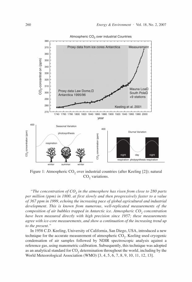
“The concentration of CO2 in the atmosphere has risen from close to 280 partsper million (ppm) in 1800, at first slowly and then progressively faster to a valueof 367 ppm in 1999, echoing the increasing pace of global agricultural and industrialdevelopment. This is known from numerous, well-replicated measurements of thecomposition of air bubbles trapped in Antarctic ice. Atmospheric CO2 concentrationhave been measured directly with high precision since 1957; these measurementsagree with ice-core measurements, and show a continuation of the increasing trend upto the present.”

In 1958 C.D. Keeling, University of California, San Diego, USA, introduced a newtechnique for the accurate measurement of atmospheric CO2. Keeling used cryogeniccondensation of air samples followed by NDIR spectroscopic analysis against areference gas, using manometric calibration. Subsequently, this technique was adoptedas an analytical standard for CO2 determination throughout the world, including by theWorld Meteorological Association (WMO) [3, 4, 5, 6, 7, 8, 9, 10, 11, 12, 13].

Proxy data from ice cores Antarctica

380

370

360

350

340

330

320

310

300CO

2-co

ncen

trat

on (

ppm

)

290

280

2701740 1760 1780 1800 1820 1840 1860

year1880 1900 1920 1940 1960 1980 2000

Proxy data Law Dome,�Antarctica 1995/96

Atmospheric CO2 over industrial Countries

Mauna Loa�South Pole�+9 stations

Keeling et al. 2001

Measurement

respiration

night nightday

photysynthesis respiration

Diurnal Variation400

CO

2 co

ncen

tratio

n (p

pm)

winter

respiration

Seasonal Variation

photosynthesis

400

CO

2 co

ncen

tratio

n (p

pm)

summer winter

Figure 1: Atmospheric CO2 over industrial countries (after Keeling [2]); natural CO2 variations.

CO2 measuring stations are distributed across the globe. Most, however, are locatedin coastal or island areas in order to obtain air without contamination from vegetation,organisms and industrial activity, i.e. to establish the so-called background level ofCO2. In considering such measurements, account should be taken of the establishedfact that land-derived air flowing seawards looses about 10 ppm of its carbon dioxideto dissolution in the oceans, and even more in colder waters (Henrys Law).

THE ESTABLISHED CRITICAL VIEW ON HISTORICAL CO2 DATAA major issue regarding the IPCC approach to linking climate and CO2 is theassumption that prior to the industrial revolution the level of atmospheric CO2 was inan equilibrium state of about 280 ppm, around which little or no variation occurred.This presumption of constancy and equilibrium is based upon a critical review of theolder literature on atmospheric CO2 content by Callendar and Keeling. (See Table 1).

Between 1800 and 1961, more than 380 technical papers that were published on airgas analysis contained data on atmospheric CO2 concentrations. Callendar [16, 20, 24]Keeling and the IPCC did not provide a thorough evaluation of these papers and thestandard chemical methods that they deployed. Rather, they discredited these techniquesand data, and rejected most as faulty or highly inaccurate [20, 22, 23, 25, 26, 27].

Though they acknowledge the concept of an ‘unpolluted background level’ forCO2, these authors only examined about 10% of the available literature, asserting fromthat that only 1% of all previous data could be viewed as accurate (Müntz [28, 29, 30],Reiset [31], Buch [32]).

THE CHALLENGE OF THE MAIN STREAM VIEW ON THE HISTORICAL DATADuring my own review of the literature, I observed that the evaluation of Reiset’s andMüntz’s work by Callendar and Keeling was erroneous. This made me investigate

180 Years of Atmospheric CO2 Gas Analysis by Chemical Methods 261

Table 1: Bibliographies and citation of papers

Cited authors and papers with data

Year Authors Total 19thc. 20thc. Notes

1900 Letts and Blake [14] 252 252 Only 19th century (+)1912 Benedict [15] 137 137 +; focus on O2 determination1940 Callendar [16] 13 7 6 Cited Letts&Blake and Benedict1951 Effenberger [17] 56 32 24 Cited Duerst1, Misra1 and Kreutz1

1952 Stepanova [18] 229 130 99 Citation as Effenberger 1956 Slocum [19] 33 22 11 Cited Duerst and Kreutz1958 Callendar [20] 30 18 12 No citing of Duerst, Kreutz and Misra 1958 Bray [21] 49 20 19 Cited most important through the centuries1986 Fraser [22] 6 6 +, same as Callendar1986 Keeling [23] 18 18 +, same as Callendar;2006 Beck [this study] 156 82 74 Only chemical determination until 19611see references

carefully the criteria that were used by these and other authors to accept or to rejectsuch historical data.

The data accepted by Callendar and Keeling had to be sufficiently low to beconsistent with the greenhouse hypothesis of climate change controlled by rising CO2emissions from fossil fuel burning. Callendar rejected nearly all data before 1870because of “relatively crude instrumentation” and reported only twelve suitable datasets in 20th century as known to him [20] out of 99 made available by Stepanova 1952[18]. The intent of these authors was to identify CO2 determinations that were madeusing pure unpolluted air, in order to assess the true background level of CO2.Callendar set out the criteria that he used to judge whether older determinations were“allowable” in his 1958 paper [20] which presents only data that fell within 10% of alonger yearly average estimated for the region, and also rejected all measurements,however accurate, that were “measurements intended for special purposes, such asbiological, soil air, atmospheric pollution”.

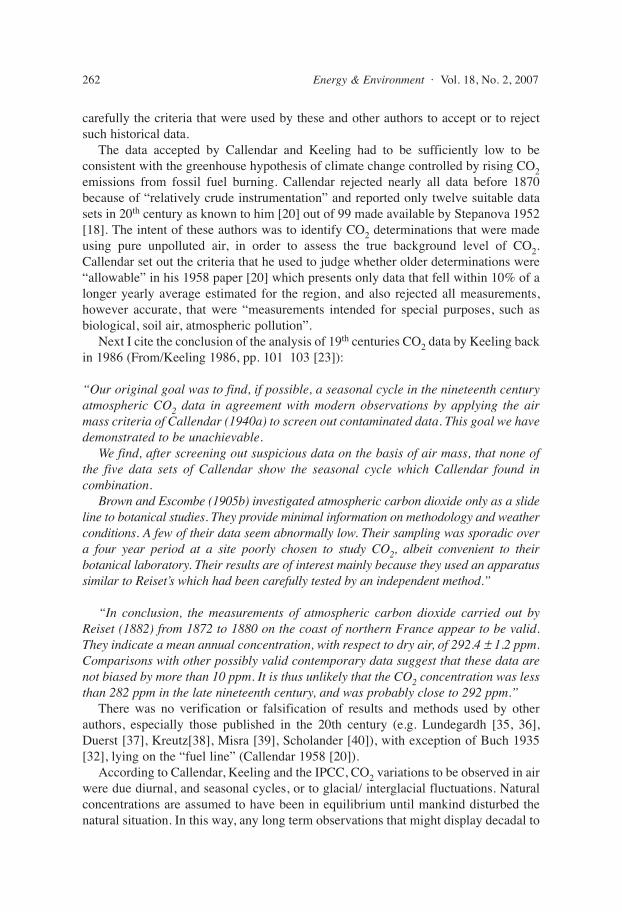
Next I cite the conclusion of the analysis of 19th centuries CO2 data by Keeling backin 1986 (From/Keeling 1986, pp. 101 103 [23]):

“Our original goal was to find, if possible, a seasonal cycle in the nineteenth centuryatmospheric CO2 data in agreement with modern observations by applying the airmass criteria of Callendar (1940a) to screen out contaminated data. This goal we havedemonstrated to be unachievable.

We find, after screening out suspicious data on the basis of air mass, that none ofthe five data sets of Callendar show the seasonal cycle which Callendar found incombination.

Brown and Escombe (1905b) investigated atmospheric carbon dioxide only as a slideline to botanical studies. They provide minimal information on methodology and weatherconditions. A few of their data seem abnormally low. Their sampling was sporadic overa four year period at a site poorly chosen to study CO2, albeit convenient to theirbotanical laboratory. Their results are of interest mainly because they used an apparatussimilar to Reiset’s which had been carefully tested by an independent method.”

“In conclusion, the measurements of atmospheric carbon dioxide carried out byReiset (1882) from 1872 to 1880 on the coast of northern France appear to be valid.They indicate a mean annual concentration, with respect to dry air, of 292.4 ± 1.2 ppm.Comparisons with other possibly valid contemporary data suggest that these data arenot biased by more than 10 ppm. It is thus unlikely that the CO2 concentration was lessthan 282 ppm in the late nineteenth century, and was probably close to 292 ppm.”

There was no verification or falsification of results and methods used by otherauthors, especially those published in the 20th century (e.g. Lundegardh [35, 36],Duerst [37], Kreutz[38], Misra [39], Scholander [40]), with exception of Buch 1935[32], lying on the “fuel line” (Callendar 1958 [20]).

According to Callendar, Keeling and the IPCC, CO2 variations to be observed in airwere due diurnal, and seasonal cycles, or to glacial/ interglacial fluctuations. Naturalconcentrations are assumed to have been in equilibrium until mankind disturbed thenatural situation. In this way, any long term observations that might display decadal to


centennial natural variations in atmospheric CO2 are ruled out a priori by Callendarand Keeling.

As I discuss further below, these criticisms by Callendar and Keeling, and theselective way in which they discarded previous data, are not able to be justified. Theirmost egregious error was perhaps the dismissal of all data which showed variations fromtheir presupposed average. That said, it is of course the case that some of the older datahas to be viewed as less reliable for technical, analytical reasons, as also indicated below.

CRITICAL SURVEY OF THE CHEMICAL METHODS APPLIED IN THE PASTIn this paper, I have assembled a 138 year-long record of yearly atmospheric CO2levels, extracted from more then 180 technical papers published between 1812 and1961. The latter year marked the end of the era of classical chemical analysis.

The compilation of data was selective. Nearly all of the air sample measurements that Iused were originally obtained from rural areas or the periphery of towns, under comparableconditions of a height of approx. 2 m above ground at a site distant from potential industrialor military contamination. Evaluation of the chemical methods used reveals systematicallyhigh accuracy, with a maximum 3% error reducing to 1% for the data of HenrikLundegardh (1920 26), a pioneer of plant physiology and ecology [34, 35, 36].

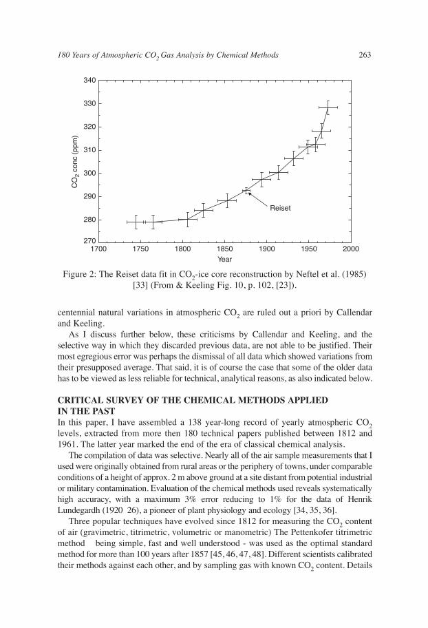
Three popular techniques have evolved since 1812 for measuring the CO2 contentof air (gravimetric, titrimetric, volumetric or manometric) The Pettenkofer titrimetricmethod being simple, fast and well understood - was used as the optimal standardmethod for more than 100 years after 1857 [45, 46, 47, 48]. Different scientists calibratedtheir methods against each other, and by sampling gas with known CO2 content. Details


340C

O2

conc

(pp

m)

330

320

310

300

290

280

2701700 1750 1800 1850

Year

Reiset

1900 1950 2000

Figure 2: The Reiset data fit in CO2-ice core reconstruction by Neftel et al. (1985)[33] (From & Keeling Fig. 10, p. 102, [23]).

of the measurement parameters, local modalities and measuring errors can be extractedfrom the available literature.

The Pettenkofer process and all its variants included the absorption of a knownvolume of air in alkaline solution (Ba(OH)2, KOH, NaOH) and titration with acid(oxalic, sulphuric, hydrochloric acid) of the produced carbonate. Basic accuracy is +/−0,0006 vol% [34, 45 ] optimized to +/−0,0003 vol% by Lundegardh [35], who providescomparative measurements with the other techniques (see table 3).

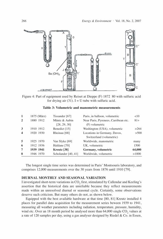
The volumetric apparatuses used before Haldane [70] and Benedict/Sonden/Petterson(e.g. 1900; [15, 44]), including gas analysers used by the French authors Regnault,Müntz, Tissander and earlier authors were open systems which lacked efficient controlof reaction temperature (see Schuftan 1933, [43,]). So their data were less reliable. MostFrench authors such as Müntz, Tissander and Reiset (Pettenkofer process) used sulphuricacid for drying air (or releasing CO2, Müntz [28, 29, 30]) before determination of CO2content. Because of the absorption of a considerable fraction of CO2 in the sulphuricacid, their values are too low (Bunsen absorption coefficient H2SO4 at 25°C = 0,96; H2Oat 25°C = 0,759; [72]). These systematic errors were known since 1848, Hlasiwetz [73]1856 and Spring [57] 1885 determined these absorption losses to 7 10% or about 20ppm.

Neither Callendar or Keeling nor the IPCC commented on these systematic errorsresulting in too low values. In fact, Reiset and Müntz were singled out for specialpraise by Keeling and IPCC as the source of the best available data of that time. [22,23, 25, 26, 27, 74] However, because of the deficiencies results determined using thesemethods have not been incorporated in the present study.

Discounting such unsatisfactory data, in every decade since 1857 we can stillidentify several measurement series that contain hundreds of precise, continuous data.

Measurements made prior to 1857 (introduction of Pettenkofer method, 3% accuracy),mostly by French authors (Boussingault, [14]; Brunner [14]; Regnault [ 14], [75]), showsystematic errors due to long connections (absorption in caoutchouc), H2SO4 for dryingair and missing temperature management. There being no calibration against Pettenkoferor modern volumetric/manometric equipment, so I cannot quantify accurately the range


Figure 3: Important historic gas analysers used by hundreds of scientists up to 1961 [26, 42, 43, 44].

of error. Well known absorption errors are in the order of 30 ppm. Amongst these authors,only de Saussure (1826-1830; [76]) measured a realistic image of the seasonal CO2 cycle.

The highest density of data was achieved by Wilhelm Kreutz at the state-of-the-artmeteorological station in Giessen (Germany) [38], using a closed, volumetric, automaticsystem designed by Paul Schuftan, the father of modern gas chromatography; [43, 78].Kreutz compiled more than 64,000 single measurements using this equipment in an18 month period during 1939 1941.


Table 2: Series of CO2 measurements since 1855 lasting more than a year using the titrimetric Pettenkofer process

Amount of Year Author Locality determinations

1 Since 1855 v. Pettenkofer [46] Munich (D) Many2 1856 (6 month)1 v. Gilm1 [50] Innsbruck1 (AUS) 193 1863 1864 Schulze2 [51] Rostock, (D) 4264 1864/65 Smith [52] London, Manchester, 246

Scotland (GB)5 1868 1871 Schulze2 [51] Rostock, (D) 16006 1872 1873 Reiset [53] Dieppe, France (Northsea) (F) 927 1873 Truchot [54] Clermont Ferrand (F) 608 1874 875 Farsky2 [55] Tabor, Böhmen, (Cz) 2959 1874 1875 Hässelbarth2 [56] Dahme (D) 347

10 1879 1880 Reiset [31] Dieppe (F) 11811 1883 Spring [57]2 Liege (B) 26612 1886 1887 Uffelmann [58] Rostock (D) 42013 1889 1891 Petermann [59] Gembloux (B) 52514 1897 1898 Letts&Blake [14] near Belfast (IRL) 6415 1898 1901 Brown& Escombe [60] Kew Garden England (GB) 9216 1917 1918 A. Krogh [61, 62] Kopenhagen (DK) Many17 1920 1926 Lundegardh [35] in southern Sweden >3000

(Kattegat) (S)18 1928 Krogh/Rehberg [62] Kopenhagen (DK) Many19 1932 1935 Buch [32] Northern atlantic ocean/ 176

Finland (FIN)20 1936 1939 Duerst [37] at Bern (Switzerland) (CH) >1000 21 1941 1943 Misra [39] Poona, India (IND) > 25022 1950 Effenberger [17] Hamburg (D) >4023 1954 Chapman et al. [63] Ames (IOWA, USA) >10024 1957 Steinhauser [64] Vienna (AUS) >50025 1955 1960 Fonselius et al. [65] Scandinavia >3400

Bischof [66]1v. Gilm: similar process as Pettenkofer, first calibrated.2identical variant of Pettenkofer process, sampling by tube through opening in window.

The longest single time series was determined in Paris’ Montsouris laboratory, andcomprises 12,000 measurements over the 30 years from 1876 until 1910 [79].

DIURNAL MONTHLY AND SEASONAL VARIATIONI investigated short-term variations in CO2 first, stimulated by Callendar and Keeling’sassertion that the historical data are unreliable because they reflect measurementsmade within an unresolved diurnal or seasonal cycle. Certainly, some observationsdeserve such criticism. But many others do not, as shown below.

Equipped with the best available hardware at that time [80, 81] Kreutz installed 4places for parallel data acquisition for the measurement series beween 1939 to 1941,measuring all weather parameters including radiation, temperature, pressure, humidity,wind etc. Over an 18 month period he analysed more than 64,000 single CO2 values ata rate of 120 samples per day, using a gas analyser designed by Riedel & Co. in Essen,


Table 3: Volumetric and manometric measurements

1 1875 (März) Tissander [67] Paris, in balloon, volumetric <102 1880 1912 Müntz & Aubin Near Paris, Pyrenees, Carribean etc. 81+

[28, 29, 30] (F) volumetric3 1910 1912 Benedict [15] Washington (USA), volumetric >2644 1920 1930 Rheinau [68] Locations in Germany, Davos, >500

Switzerland (volumetric)5 1925 1970 Van Slyke [69] Worldwide, manometric many6 1912 1936 Haldane [70] UK, volumetric 15007 1939 1941 Kreutz [38] Germany, volumetric 64,0008 1946 1970 Scholander [40, 41] Worldwide, volumetric >1000

T

JBa (OH)2

F

I

T

B′

B′

B

C′

C

C′′II

0

A

t ′

t

Figure 4: Part of equipment used by Reiset at Dieppe (F) 1872 80 with sulfuric acidfor drying air (31). I = U-tube with sulfuric acid.

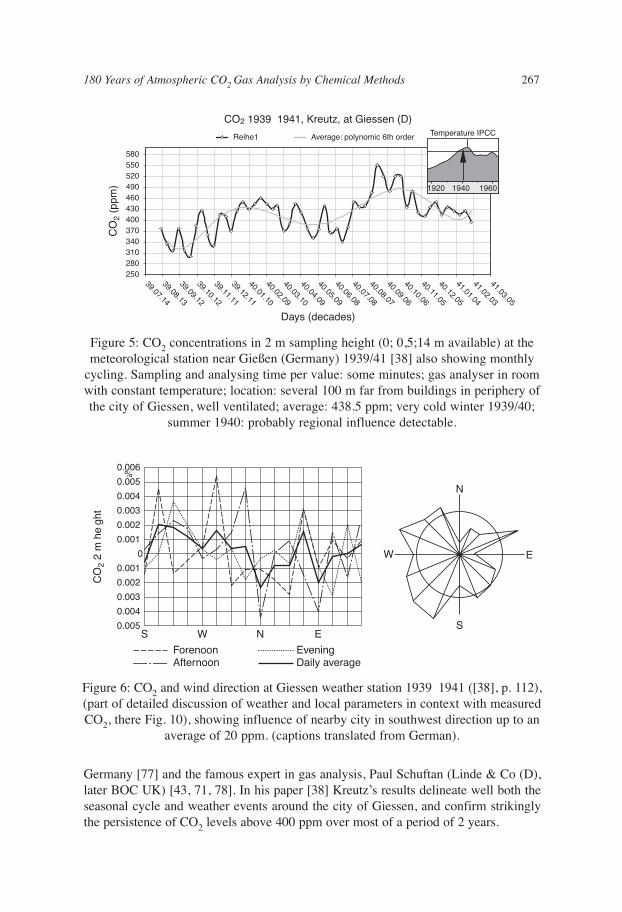
Germany [77] and the famous expert in gas analysis, Paul Schuftan (Linde & Co (D),later BOC UK) [43, 71, 78]. In his paper [38] Kreutz’s results delineate well both theseasonal cycle and weather events around the city of Giessen, and confirm strikinglythe persistence of CO2 levels above 400 ppm over most of a period of 2 years.


580550520490460430400370C

O2

(ppm

)

340310280250

39.07.14

39.08.13

39.09.12

39.10.12

39.11.11

39.12.11

40.01.10

40.02.09

40.03.10

40.04.09

40.05.09

40.06.08

40.07.08

40.08.07

40.09.06

40.10.06

40.11.05

40.12.05

41.01.04

41.02.03

41.03.05

Average: polynomic 6th orderReihe1

Days (decades)

CO2 1939 1941, Kreutz, at Giessen (D)

1920 19601940

Temperature IPCC

Figure 5: CO2 concentrations in 2 m sampling height (0; 0,5;14 m available) at themeteorological station near Gießen (Germany) 1939/41 [38] also showing monthly

cycling. Sampling and analysing time per value: some minutes; gas analyser in roomwith constant temperature; location: several 100 m far from buildings in periphery ofthe city of Giessen, well ventilated; average: 438.5 ppm; very cold winter 1939/40;

summer 1940: probably regional influence detectable.

Forenoon

0.006

0.005%

0.004

0.003

0.002

0.001

0

0.001

CO

2 2

m h

egh

t

0.002

0.003

0.004

0.005S W N E

AfternoonEvening

S

W

N

E

Daily average

Figure 6: CO2 and wind direction at Giessen weather station 1939 1941 ([38], p. 112),(part of detailed discussion of weather and local parameters in context with measuredCO2, there Fig. 10), showing influence of nearby city in southwest direction up to an

average of 20 ppm. (captions translated from German).

The overall average CO2 level for the 25,000 values plotted from Giessen is 438.5ppm. This figure needs to be adjusted downwards to take account of anthropogenicsources of CO2 from nearby city, an influence that has been estimated as lying between10 and 70 ppm (average 30 ppm) by different authors (61, 57, 82, 83).

Even after making this adjustment, the Giessen results strongly contradict modern(IPCC) estimates of carbon dioxide levels during the 1940s. These results of Kreutzwere not cited or evaluated by Callendar and Keeling. Others, who have mentioned thework, such as Slocum [19], Effenberger [17] and Bray [21], invariably give faultycitation of the details.

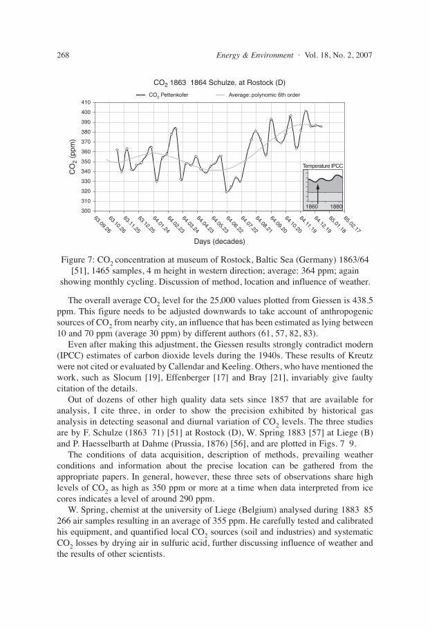
Out of dozens of other high quality data sets since 1857 that are available foranalysis, I cite three, in order to show the precision exhibited by historical gasanalysis in detecting seasonal and diurnal variation of CO2 levels. The three studiesare by F. Schulze (1863 71) [51] at Rostock (D), W. Spring 1883 [57] at Liege (B)and P. Haesselbarth at Dahme (Prussia, 1876) [56], and are plotted in Figs. 7 9.

The conditions of data acquisition, description of methods, prevailing weatherconditions and information about the precise location can be gathered from theappropriate papers. In general, however, these three sets of observations share highlevels of CO2 as high as 350 ppm or more at a time when data interpreted from icecores indicates a level of around 290 ppm.

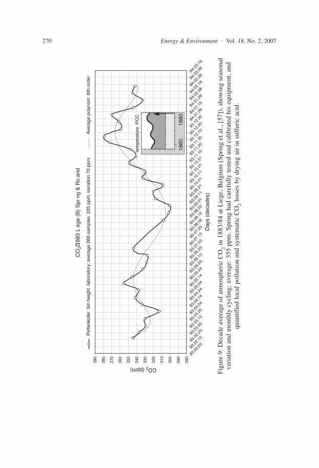
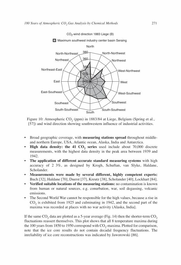
W. Spring, chemist at the university of Liege (Belgium) analysed during 1883 85266 air samples resulting in an average of 355 ppm. He carefully tested and calibratedhis equipment, and quantified local CO2 sources (soil and industries) and systematicCO2 losses by drying air in sulfuric acid, further discussing influence of weather andthe results of other scientists.


1860 1880

Temperature IPCC

63.09.26

410

400

390

380

370

360

350

340

330

320

310

30063.10.26

63.11.25

Days (decades)

CO

2 (p

pm)

63.12.25

64.01.24

64.02.23

64.03.24

64.04.23

64.05.23

64.06.22

64.07.22

64.08.21

64.09.20

64.10.20

64.11.19

64.12.19

65.01.18

65.02.17

CO2 1863 1864 Schulze, at Rostock (D)

Average: polynomic 6th orderCO2 Pettenkofer

Figure 7: CO2 concentration at museum of Rostock, Baltic Sea (Germany) 1863/64[51], 1465 samples, 4 m height in western direction; average: 364 ppm; again

showing monthly cycling. Discussion of method, location and influence of weather.

More historic measurement series include evaluation of methods and locations,are being prepared for publication. Here I also point out a remarkable observation,which also can be made from the recent Mauna Loa data and others, which passed sofar apparently not acknowledged, that superposed on all seasonal variations, is anothermonthly variation with a wave length of 28 30 days.

COMPILATION OF THE HISTORICAL DATAIn this section I present the analytical data over a 150 year period for air gas analysisdetermined by classical chemical techniques, as published in 138 scientific papers. Thedata presented have been retained unmodified. They mostly comprise measurementsmade on samples collected at a height of approx. 2 (or some) m above ground, fromstations located throughout the northern hemisphere, from Alaska, through Europe, toPune (India).

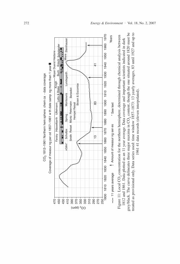
Firstly a raw picture is presented in figure 11 over the period 1812 1961 with 11 yearssmoothing (11 year moving average filter [85]):

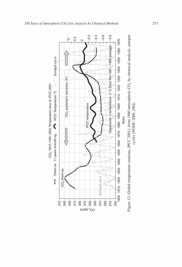
Figure 12 shows a comparison between the eleven years-averaged CO2 curve andthe IPCC (2001) annually averaged temperature record between 1860 and 2000. Short-term fluctuations in CO2 are suppressed by the filtering, but at the broad level there isa close match between the 1942’s peaks for CO2 and temperature.

Subsequent figure 13 presents a raw picture out of 41 yearly averages over theperiod 1920 1961 compared to ice core records by Neftel et al. [33].

Notice that the peak CO2 content and peak temperature coincide in 1942, anobservation which will be given more attention below. The overall validity of the patternof CO2 fluctuations is supported by the following considerations.


440

410

380

350

320

290

260

230

2004:48 9:36 14:24 19:12

Time

0:00 4:48 9:36 14:24

CO2 (ppm), Pettenkofer variant, 34 L air, every 3 h., 1m table in garden, no wind, no clouds

Diurnal CO2, 24th - 25th July 1876, Dahme, Hässelbarth

CO

2 (p

pm)

Figure 8: Diurnal variation of atmospheric CO2 on 24th/25th July 1876, in peripheryof the small rural town of Dahme (Prussia, Germany, center of agricultural activities)

[56] measured in the stations garden showing respiration of plants and lackingphotosynthesis at night; sampling and analysing time: 3 hours; average: 322 ppm.

83.0

2.0383

.02.

1383.0

2.23

CO2 (ppm)

Day

s (d

ecad

es)

CO

2�18

83 L

ege

(B)

Spr

ng &

Ro

and

390

380

370

360

350

340

330

320

310

300

290

280

83.0

3.0583

.03.

1583.0

3.2583

.04.

0483.0

4.1483

.04.

2483.0

5.0483

.05.

1483.0

5.2483

.06.

0383.0

6.1383

.06.

2383.0

7.0383

.07.

1383.0

7.2383

.08.

0283.0

8.1283

.08.

2283.0

9.0183

.09.

1183.0

9.2183

.10.

0183.1

0.1183

.10.

2183.1

0.3183

.11.

1083.1

1.2083

.11.

3083.1

2.1083

.12.

2083.1

2.3084

.01.

0984.0

1.1984

.01.

2984.0

2.0884

.02.

1884.0

2.2884

.03.

0984.0

3.19

tem

pera

ture

PC

C

1860

1880

Pet

tenk

ofer

5m

hei

ght

labo

rato

ry; a

vera

ge 2

66 s

ampl

es 3

35 p

pm; v

aria

tion

70 p

pmA

vera

ge p

olyn

om 6

th o

rder

Figu

re 9

: Dec

ade

aver

age

of a

tmos

pher

ic C

O2

in 1

883/

84 a

t Lie

ge, B

elgi

um (

Spri

ng e

t al.,

[57

]), s

how

ing

seas

onal

vari

atio

n an

d m

onth

ly c

yclin

g; a

vera

ge: 3

55 p

pm. S

prin

g ha

d ca

refu

lly te

sted

and

cal

ibra

ted

his

equi

pmen

t, an

dqu

antif

ied

loca

l pol

lutio

n an

d sy

stem

atic

CO

2lo

sses

by

dryi

ng a

ir in

sul

furi

c ac

id.


• Broad geographic coverage, with measuring stations spread throughout middle-and northern Europe, USA, Atlantic ocean, Alaska, India and Antarctica.

• High data density: the 41 CO2 series used include about 70,000 discretemeasurements, with the highest data density in the peak area between 1939 and1942.

• The application of different accurate standard measuring systems with highaccuracy of 2 3%, as designed by Krogh, Schuftan, van Slyke, Haldane,Scholander.

• Measurements were made by several different, highly competent experts:Buch [32], Haldane [70], Duerst [37], Kreutz [38], Scholander [40], Lockhart [84].

• Verified suitable locations of the measuring stations: no contamination is knownfrom human or natural sources, e.g. conurbation, war, soil degassing, volcanicemissions.

• The Second World War cannot be responsible for the high values, because a rise inCO2 is exhibited from 1925 and culminating in 1942, and the second part of themaxima was recorded at places with no war activity (Alaska, India].

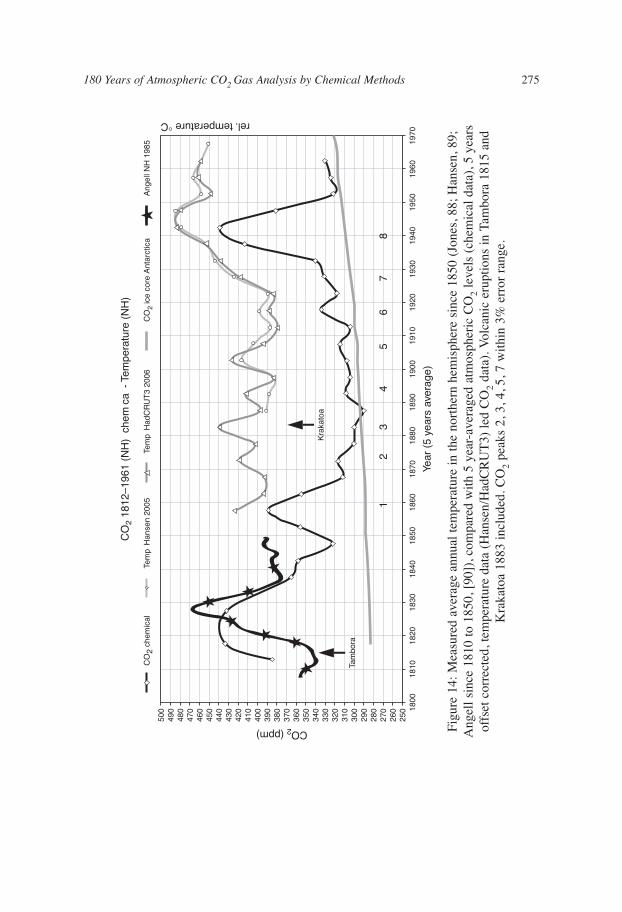
If the same CO2 data are plotted as a 5-year average (Fig. 14) then the shorter-term CO2fluctuations reassert themselves. This plot shows that all 8 temperature maxima duringthe 100 years from 1850 to 1950 correspond with CO2-maxima. Plotted for comparison,note that the ice core results do not contain decadal frequency fluctuations. Theinreliability of ice core reconstructions was indicated by Jaworowski [86].


SouthSouth-Southwest

Southwest

West-Southwest

West

West-Northwest

Northwest

North-Northwest

North

380

360

340

320

300

North-Northeast

CO2-wind direction 1883 Liege (B)

Northeast

Northeast-East

East

East-Southeast

Southeast

South-Southeast

Maximum southwest industry center basin Seraing

Figure 10: Atmospheric CO2 (ppm) in 1883/84 at Liege, Belgium (Spring et al.,[57]) and wind direction showing southwestern influence of industrial activities.

1800 11

yea

rs a

vera

ge

CO2 (ppm)

Am

ount

of m

easu

rng

sere

s*

See

text

470

450

430

410

390

370

350

1383

Fars

ky

vGilm

*

Sm

ithR

eise

tM

üntz

Pet

erm

ann

Ben

edic

tH

empe

l Rei

set

Bro

wn

& E

scom

be

Sch

ultz

eS

prin

gM

onts

ouris

Lund

egar

dhM

isra

Ste

inha

user

Häs

selb

arth

Uffe

lman

nLe

tts &

Bla

keKro

ghB

uch

Kre

utz

Sch

olan

der

41

330

310

290

270

250

1810

1820

1830

1840

1850

1860

1870

1880

1890

1900

1910

1920

1930

1940

1950

1960

1970

Year

s

Moy

er D

uers

t Hal

dane

Cov

erag

e of

mea

surn

g pe

rod

1857

–196

1 w

th d

ate

sam

png

mor

e th

an 1

yea

r

CO

2 18

12–1

961

Nor

ther

n he

msp

here

che

mca

- d

ata

cove

rage

Figu

re 1

1: L

ocal

CO

2 co

ncen

trat

ion

for

the

nort

hern

hem

isph

ere,

det

erm

ined

thro

ugh

chem

ical

ana

lysi

s be

twee

n18

12 a

nd 1

861.

Dat

a pl

otte

d as

an

11 y

ear

aver

age.

Dat

a co

vera

ge a

nd im

port

ant s

cien

tists

indi

cate

d in

dar

kgr

ey/b

lack

. The

cur

ve d

elin

eate

s th

ree

maj

or m

axim

a in

CO

2co

nten

t, th

ough

the

one

situ

ated

aro

und

1820

mus

t be

trea

ted

as p

rovi

sion

al o

nly.

Dat

a se

ries

use

d: ti

me

win

dow

185

7–18

73: 1

3 ye

arly

ave

rage

s, 8

3 un

til 1

927

and

up to

1961

41

data

rec

ords

(el

even

inte

rpol

ated

).


470

540

430

410

390

370

350

330

310

290

270

250 18

00

CO2 (ppm)

1810

1820

1830

1840

1850

1860

1870

1880 Ye

ars

CO

2 18

12–1

961

(NH

) Tem

pera

ture

(w

ord)

IPC

C 2

001

Sun

spot

cyc

e

IPC

C te

mpe

ratu

re

Dep

artu

res

n te

mpe

ratu

re n

°C

(fr

om th

e 19

61 -

199

0 av

erag

e)

°C 02

0 –0

2

–0

4

–0

6

–0

8

CO

2 sy

stem

atc

accu

racy

: 3%

CO

2 ch

emca

1890

1900

1910

1920

1930

1940

1950

1960

1970

Che

mca

11

year

s sm

ooth

ngIP

CC

Tem

pera

ture

°C

Sun

spot

cyc

e

Figu

re 1

2: G

loba

l tem

pera

ture

(st

atio

ns, I

PCC

200

1), f

rom

186

0 at

mos

pher

ic C

O2

by c

hem

ical

ana

lysi

s, s

unsp

otcy

cles

(N

GD

C 2

006,

[96

]).


490

CO

2 19

20–1

961

Nor

ther

n he

msp

here

che

mca

Ice

core

Ant

arct

caC

O2

chem

caTe

mpe

ratu

re IP

CC

CO2 (ppm)

470

450

430

410

390

370

350

330

310

290

270

290 19

1519

2019

25

Lund

gard

hV

an s

yke

Ha

dane

Due

rst

Kre

utz

Msr

a

Sch

oan

der

1930

1935

1940

Year

1945

1950

1955

1960

1965

1940

1960

1920

Figu

re 1

3: T

he n

orth

ern

hem

isph

ere

1942

CO

2m

axim

um, d

elin

eate

d by

his

tori

cal c

hem

ical

ana

lysi

s. I

nclu

sive

ice

core

dat

a by

Nef

tel e

t al.

[33]

and

IPC

C te

mpe

ratu

re f

or o

rien

tatio

n.


500

490

480

470

460

450

440

430

420

410

400

390

380

370

360

350

340

330

320

310

300

290

280

270

260

250 18

0018

1018

2018

3018

4018

5018

6018

70 Year

(5

year

s av

erag

e)

CO

2 18

12–1

961

(NH

) c

hem

ca -

Tem

pera

ture

(N

H)

rel. temperature °C

CO2 (ppm)

1880

1890

1900

1910

1920

1930

1940

1950

1960

1970

Kra

kato

a

Tam

bora

12

34

56

78

CO

2 ch

emic

alTe

mp

Han

sen

2005

Tem

p H

adC

RU

T3

2006

CO

2 ic

e co

re A

ntar

ctic

aA

ngel

l NH

198

5

Figu

re 1

4: M

easu

red

aver

age

annu

al te

mpe

ratu

re in

the

nort

hern

hem

isph

ere

sinc

e 18

50 (

Jone

s, 8

8; H

anse

n, 8

9;A

ngel

l sin

ce 1

810

to 1

850,

[90

]), c

ompa

red

with

5 y

ear-

aver

aged

atm

osph

eric

CO

2le

vels

(ch

emic

al d

ata)

, 5 y

ears

offs

et c

orre

cted

, tem

pera

ture

dat

a (H

anse

n/H

adC

RU

T3)

led

CO

2da

ta).

Vol

cani

c er

uptio

ns in

Tam

bora

181

5 an

dK

raka

toa

1883

incl

uded

. CO

2pe

aks

2, 3

, 4, 5

, 7 w

ithin

3%

err

or r

ange

.


The close relationship between temperature change and CO2 level exhibited by theseresults is consistent with a cause-effect relationship, but does not of itself indicate whichof the two parameters is the cause and which the effect. The greenhouse hypothesis ofIPCC argues for CO2 being the cause (through radiative feedback) of the temperaturerise. My results are equally if not more consistent with temperature being the forcing thatcontrols the level of CO2 in the atmospheric system. In support of this causality, ice-coredata consistently shows that over climatic time scales, changes in temperature precedetheir parallel changes in carbon dioxide by several hundred to more than a thousandyears [91].

Most of the historical chemical measurements were accomplished on samplescollected from the boreal regions of the northern hemisphere. Here, the diurnal andseasonal variation in atmospheric CO2 displays a much higher amplitude than is thecase for oceanic areas, where smoothing influences result in a diminution of CO2 levelsby 10 ppm or more. An imbalance of photosynthesis, respiration and soil respiration inand near to forests may lead to periodic emissions of large quantities of CO2 [83, 92].Substantial differences in amplitude of parts of the carbon cycle is well known in thenorthern hemisphere (e.g. methane [93]; Luxembourg, [94]). Such effects may explainthe various smaller fluctuations in CO2 content through the historical chemical record,which are not imaged by ice cores or at ocean stations.

DISCUSSION AND CONCLUSIONSDuring the late 20th century, the hypothesis that the ongoing rise of CO2 concentrationin the atmosphere is a result of fossil fuel burning became the dominant paradigm. Toestablish this paradigm, and increasingly since then, historical measurements indicatingfluctuating CO2 levels between 300 and more than 400 ppmv have been neglected.

A re-evaluation has been undertaken of the historical literature on atmospheric CO2levels since the introduction of reliable chemical measuring techniques in the early tomiddle 19th century. More than 90,000 individual determinations of CO2 levels arereported between 1812 and 1961. The great majority of these determinations weremade by skilled investigators using well established laboratory analytical techniques.Data from 138 sources and locations have been combined to produce a yearly averageatmospheric CO2 curve for the northern hemisphere.

The historical data that I have considered to be reliable can, of course, bechallenged on the grounds that they represent local measurements only, and aretherefore not representative on a global scale. Strong evidence that this is not the case,and that the composite historical CO2 curve is globally meaningful, comes from thecorrespondence between the curve and other global phenomena, including bothsunspot cycles and the moon phases, the latter presented here probably first time inliterature and the average global temperature statistic. Furthermore, that the historicaldata are reliable in themselves is supported by the credible seasonal, monthly and dailyvariations that they display, the pattern of which corresponds with modernmeasurements. It is indeed surprising that the quality and accuracy of these historicCO2 measurements has escaped the attention of other researchers.

How to interpret the monthly variation of CO2 (see Fig. 5, 7, 9 and modernmeasurements e.g. Mauna Loa), which indicates a coincidence with the lunar phases,is another question to be dealt within a paper in preparation.


Modern greenhouse hypothesis is based on the work of G.S. Callendar and C.D.Keeling, following S. Arrhenius, as latterly popularized by the IPCC. Review ofavailable literature raise the question if these authors have systematically discarded alarge number of valid technical papers and older atmospheric CO2 determinationsbecause they did not fit their hypothesis? Obviously they use only a few carefullyselected values from the older literature, invariably choosing results that are consistentwith the hypothesis of an induced rise of CO2 in air caused by the burning of fossilfuel. Evidence for lacking evaluation of methods results from the finding that asaccurate selected results show systematic errors in the order of at least 20 ppm [28, 29,30, 31, 57, 73]. Most authors and sources have summarised the historical CO2determinations by chemical methods incorrectly and promulgated the unjustifiableview that historical methods of analysis were unreliable and produced poor qualityresults [2, 20, 22, 23, 24, 25, 26, 27, 65, 74, 95].

ACKNOWLEDGEMENTSThe author wishes to give special thanks to the following individuals for their help inobtaining the historical information:Dr. L. Brake, archive of the city of Giessen (D]Jana Farová, Infocentrum Mesto Tábor, (Cz]Dr. Haus, archivist Buderus company at Wetzlar (D]Ralph-Christian Mendelsohn, German Weather Wervice (DWD], Offenbach (D]Dr. Franziska Rogger, archive university of Bern (CH]Prof. Dr. Albrecht Vaupel, coworker of W. Kreutz, RWD/ DWD (D]Dr. W. Wranik, Institute of Biosciences, Marine Biology Rostock (D]

I am especially indepted toProf. Dr. Arthur Roersch, Dr. Hans Jelbring, Andre Bijkerk and Prof. Dr. BobCarter for helpful discussions, Prof. Dr. Arthur Roersch, Dr. Hans Jelbring forhelping to produce a condensed draft and Prof. Dr. Arthur Roersch and Prof. Dr.Bob Carter for their linguistic support.

REFERENCES1. Keeling, C.D., THE INFLUENCE OF MAUNA LOA OBSERVATORY ON THE

DEVELOPMENT OF ATMOSPHERIC CO2 RESEARCH; Scripps Institution ofOceanography; University of California at San Diego, 1978http://www.mlo.noaa.gov/HISTORY/PUBLISH/ 20th%20anniv/co2.htm

2. IPCC Third Assessment Report: Climate Change 2001: The Scientific Basis, J. T. Houghton,Y. Ding, D.J. Griggs, M. Noguer, P. J. van der Linden and D. Xiaosu (Eds.) CambridgeUniversity Press, UK. pp 944. http://www.unep.no/climate/ipcc tar/wg1/index.htm

3. Dickson, A. G., Reference Materials For Oceanic CO2 Measurements, Scripps Institution ofOceanography University of California, San Diego, La Jolla California USA; Unesco 1991

4. Bate, G. C., D’’Aoust, A., and Canvin; D. T., Calibration of Infra red CO2 Gas Analyzers,aDepartment of Biology, Queen’’s University, Kingston, Ontario, Canada, 1969. http://www.pubmedcentral.gov/articlerender.fcgi?artid=396226

5. AEROCARB Research Station Italy, Mt. Cimone, ISAC National Research Councilhttp://www.aerocarb.cnrs gif.fr/sites/ifa/monte cimone/monte cimone.html


6. Zhao, C.L., P.P. Tans, and K.W. Thoning, A high precision manometric system for absolutecalibrations of CO2 in dry air, Journal of Geophysical Research, 102 (D 5), 5885, 1997.

7. Scriptum Meereschemische Analytik””, WS 2002/2003; Körtzinger, Arne, University ofKiel, Germany http://www.ifm.uni kiel.de/fb/fb2/staff/Koertzinger/files/MeereschemischeAnalytik/meereschem analytik DIC.pdf

8. A High Precision Manometric System for Absolute Calibrations of CO2 Reference Gasep.NOAA/ESRL Global Monitoring Division 325 Broadway R/GMD1; Boulder, CO80305 3328 http://www.cmdl.noaa.gov/ccgg/refgases/manometer.html

9. Climate Science Pioneer: Charles David Keeling Scripps Institution of Oceanography, UCSan Diego http://sio.ucsd.edu/keeling/

10. Keeling, C.D.. The concentration and isotopic abundance of carbon dioxide in theatmosphere. Tellus 1960,12:200 203.

11. Keeling C. D., THE INFLUENCE OF MAUNA LOA OBSERVATORY ON THE DEVELOPMENT OF ATMOSPHERIC CO2 RESEARCH; Scripps Institution of Oceanography;University of California at San Diego http://www.mlo.noaa.gov/HISTORY/PUBLISH/20th%20anniv/co2.htm

12. Keeling, C.D. and T.P. Whorf. 2005. Atmospheric CO2 records from sites in the SIO airsampling network. In Trends: A Compendium of Data on Global Change. Carbon DioxideInformation Analysis Center, Oak Ridge National Laboratory, U.S. Department of Energy,Oak Ridge, Tenn., U.S.A. http://cdiac.ornl.gov/trends/co2/sio mlo.htm

13. WORLD METEOROLOGICAL ORGANIZATION GLOBAL ATMOSPHERE WATCH No.143; GLOBAL ATMOSPHERE WATCH MEASUREMENTS GUIDE; 2001/2003 http://www.wmo.ch/web/arep/reports/gaw143.pdf and http://www.wmo.ch/web/arep/reports/gaw148.pdf

14. Letts E., Blake R., The carbonic anhydride of the atmosphere; Roy. Dublin Soc. Sc.Proc.,N. P., Vol. 9, 1899 1902; Scientific Proceedings of the Royal Dublin Society

15. Benedict, F. G. “The composition of the atmosphere,” Carnegie Publication, No. 166,Washington, 1912.

16. Callendar, G. P., “Variations of the Amount of Carbon Dioxide in Different Air Currents,”Quarterly Journal of the Royal Meteorological Society, vol. 66, No. 287, October 1940, pp. 395 400.

17. Effenberger, E., “Messmethoden zur Bestimmung des C02 Gehaltes der Atmosphare unddie Bedeutung derartiger Messungen für die Biometeorologie und Meteorologie,” Annalender Meteorologie, Vierter Jahrgang, Heft 10 bis 12, 1951, pp. 417 427.

18. Stepanova, Nina A. “A Selective Annotated Bibliography of Carbon Dioxide in theAtmosphere,” Meteorological Abstracts 3: 137 170, 1952.

19. Slocum, G. HAS THE AMOUNT OF CARBON DIOXIDE IN THE ATMOSPHERECHANGED SIGNIFICANTLY SINCE THE BEGINNING OF THE TWENTIETHCENTURY, Monthly Weather Review: Vol. 83, No. 10, pp. 225 231, 1955.

20. Callendar, G.P. “On the Amount of Carbon Dioxide in the Atmosphere,” Tellus 10: 243 48.(1958).


21. Bray, J., An analysis of the possible recent Change in Atmospheric Carbon DioxideConcentration, Tellus XI 1959, 2, S 220.

22. Fraser et al., in “The changing Carbon Cycle,” Springer Verlag 1986, p. 66.

23. From, E., Keeling C. D. “Reassessment of Late 19th Century Atmospheric Carbon DioxideVariations,” Tellus, 38B: 87 105, 1986.

24. Callendar, G.P. “The Artificial Production of Carbon Dioxide and Its Influence on Climate,”Quarterly J. Royal Meteorological Society 64: 223 40, 1938.

25. Wigley, T., The Preindustrial Carbon Dioxide Level; Climate Change 5, P. 315 320, 1983.

26. The Pre 1958 Atmospheric Concentration of Carbon Dioxide; EOS Meeting June 26, 1984P. 415.

27. WPC 53, WMO Report of the Meeting in the CO2 Concentrations from pre industrialTimes I.G.Y 1983.

28. Müntz, A., Aubin, E., Ann. Chim. Phyp. Serie 5, T.26, 1882, p 222.

29. MüntzA., Aubin,E., Recherches sur les Proportions d’acide carbonique contenues dans l’air,Ann. Chim. Phyp. Serie 5, T.26, 1882, P. 222.

30. Müntz A., Aubin, E., L’acide carbonique de l’air, La Nature, Paris, 1882 , 2. Jahr, P. 385http://cnum.cnam.fr/CGI/page.cgi?4KY28.18/399/

31. Reiset, J., Recherches sur la proportion de l’acide carbonique dans l’air; Annales de Chimie(5), 26 1882, p. 144.

32. Buch, E., “Der Kohlendioxydgehalt der Luft als Indikator der MeteorologischenLuftqualitat,” Geophysica, vol. 3, 1948, p. 63 79.

33. Neftel, A. et al. Ice core sample measurements give atmospheric CO2 content during the past40,000 yr. Nature 295:220 223, 1982.

34. Lundegardh, H., Neue Apparate zur Analyse des Kohlensäuregehalts der Luft, Biochem.Zeitschr. Bd. 131, 1922, S 109.

35. Lundegardh, H., Der Kreislauf der Kohlensäure in der Natur. Fischer, Jena, (680), 1924.

36. Larkum, A., Contributions of Henrik Lundegårdh; Photosynthesis Research 76: 105 110,2003. Biography H. Lundegardh: http://www.life.uiuc.edu/govindjee/Part2/09 Larkum.pdf

37. Duerst, U., “Neue Forschungen über Verteilung und Analytische Bestimmung derwichtigsten Luftgase als Grundlage für deren hygienische und tierzüchterische Wertung,”Schweizer Archiv fiir Tierheilkunde, vol. 81, No. 7/8, August 1939, p. 305 317.

38. Kreutz, W., “Kohlensäure Gehalt der unteren Luftschichten in Abhangigkeit vonWitterungsfaktoren,” Angewandte Botanik, vol. 2, 1941, pp. 89 117.

39. Misra , R.K., Studies on the Carbon dioxide factor in the air and soil layers near the ground,Indian Journal of Meteorology and Geophysics, Vol I, No. 4, p. 127.

40. Scholander; P. F., ANALYZER FOR ACCURATE ESTIMATION OF RESPIRATORYGASES IN ONE HALF CUBIC CENTIMETER SAMPLES; J. Biol. Chem. 1947 167:235 250. http://www.jbc.org/cgi/reprint/167/1/235


41. Hock et al.; Composition of the ground level atmosphere at Point Barrow. Journal ofmeteorology, Vol 9, 1952, P. 441

42. Abderhalden, Handbuch der biochemischen Arbeitesmethoden, Berlin 1919, p. 480 undTreadwell, F.P. Kurzes Lehrbuch der analytischen Chemie, II. Band; Wien 1949, S. 511

43. Schuftan, P., Chem. Fabrik, Nr. 51, 1933, P. 513.

44. Pettersson, 0. & Sonden, K.. Skand. Arch. Physiol., 1895, 6, 16.

45. Kauko, Y., Mantere ; V. ,Eine genaue Methode zur Bestimmung des CO2 Gehaltes der LuftZeitschrift für anorganische und allgemeine Chemie. Volume 223, Issue 1, 1935. Pages33 44.

46. Pettenkofer; M., “Über eine Methode die Kohlensäure in der atmosphärischen Luft zubestimmen,” Chem. Soc. Journ. Tranp. 10 (1858), P. 292 und Journ. Prakt. Chem. 85, 1862, p.165.

47. Pettenkofer, M. und Voit, C., Zeitschrift für Biologie, 1866, 2, P. 459.

48. Pettenkofer, M., Ann. Chem. Pharm., 1862, Suppl. Bd. 2, I.

49. The respiration apparatus by M. Pettenkofer; Letter exchange by Dr. Eugen Freih. vonGorup Besanez. http://gorup.heim.at/Briefe/Pettenkofer.htm

50. v.Gilm, H., Über die Kohlensäurebestimmung der Luft Sitzungsberichte d. kaiserl.Akademie d. Wissenschaften Volume 24, 1857.

51. Schulze, F., Landw. Versuchsstationen, Vol. 9, 1867, p. 217; Vol. 10, 1868, p. 515, Vol. 12,1875 p. 1, Vol. 14, 1871, p. 366.

52. Smith, S., On the composition of the atmosphere; Manchester Lit. Phil. Soc. Proc., 1865,Vol 4, p. 30.

53. Reiset, J.A., Compt. Rend., T. 88, p. 1007, T. 90, p.1144 1457, 1879 1880.

54. Truchot, P. Sur la proportion d’acide carbonique existent dans l’air atmospherique, Compt.Rend., 77, 1873, p. 675.

55. Farsky, F., Bestimungen der atmosphärischen Kohlensäure in den Jahren 1874 1875 zuTabor in Böhmen, Wien, Akadem. Sitzungsberichte, 74, 1877, Abt. 2, p. 67.

56. Hässelbarth P., Fittbogen, J., Beobachtungen über lokale Schwankungen imKohlensäuregehalt der atmosphärischen Luft, Landw. Jahrbücher, 8, 1879, p. 669.

57. Spring, W., Roland, L. Untersuchungen über den Kohlensäuregehalt der Luft; ChemischesCentralblatt Nr. 6, 10.2.1886, 3. Folge 17. Jahrgang and Mémoires couronnés par l′Academie royal de Belgique, 37, 1885, p. 3.

58. Uffelmann, J. Luftuntersuchungen, Archiv f. Hygiene, 1888, P. 262.

59. Petermann, A., Acide carbonique contenu dans l’air atmospherique, Brux. Mem. Cour., T.47, 1892 93, 2. Abt. P. 5.

60. Brown H. , Escombe; F., On the variation in the amount of Carbon Dioxide in the Air ofKew during the Years 1898 1901; Proc. Roy. Soc., B. 76, 1905, p. 118.

61. Krogh, A., A Gas Analysis Apparatus Accurate to 0˙001% mainly designed for RespiratoryExchange Work; Biochem J. 1920 July; 14(3 4): 267 281.


62. Krogh, A., Rehberg, P. “CO2 Bestimmung in der atmosphärischen Luft durchMikrotitration,” Biochemische Zeitschrift, 1929, 205, p. 265.

63. Chapman, H. et al., The carbon dioxide content of field air, Plant Physiology 1956, Vol 29, p. 500.

64. Steinhauser, F. Der Kohlendioxidgehalt der Luft in Wien und seine Abhängigkeit vonverschiedenen Faktoren, Berichte des deutschen Wetterdienstes, Nr. 51, S 54, 1958.

65. Fonselius, S., Microdetermination of CO2 in the air, with current Data for Scandinavia,Tellus 7, 1955, pp. 259 265.

66. Bischof, W., 1960: Periodical variations of the atmospheric CO, content in Scandinavia.Tellus, 12:216 226.

67. Tissandier, G., Dosage de l’acide carbonique, de l’air a bord du ballon le Zenith, Comt.Rend. 80, 1875, p. 976.

68. Rheinau, E. Praktische Kohlensäuredüngung in Gärtnerei und Landwirtschaft, SpringerVerlag Berlin, 1927.

69. Van Slyke D. D., et al., Manometric analysis of Gas Mixtures, I,II Biol. Chem. 95 (2): P. 509und 531. http://www.jbc.org/cgi/reprint/95/2/531

70. Haldane, J. P., Methods of Air Analysis, London, 1912.

71. Schuftan, P., “Gasanalyse in der Technik,’’ P. Hirzel Verlag,. Leipzig. (1931).

72. IUPAC NIST Solubility database; http://srdata.nist.gov/solubility/sol detail.asp?sys ID=62 79.

73. Hlasiwetz, W, Über die Kohlensäurebestimmung der atmosphärischen Luft, Wien akad.Sitzungsberichte Vol. 20, 1856, p. 18.

74. Keeling, C.D., Atmospheric Carbon Dioxide in the 19th Century, Science, 202, P. 1109,1978.

75. Regnault, V., Reiset, J. (1849]. Ann. Chim. (Phyp.), 26 (3), 299.

76. de Saussure; T., Sur la variation de l’acide de carbonique atmosphérique. Annales de Chimieet Physique, 44,1830, P. 5.

77. Riedel, F.; Deutsche Patentschrift Nr. 605333, 18.10.1934; Gasuntersuchungsapparat.

78. Paul Schuftan and the early develeopment of gas adsorption chromatography; Journal ofhigh resolution chromatography, Vol. 8, Issue 10, S 651 658, 1985.

79. Stanhill, G., The Montsouris series of Carbon dioxide Concentration Measurements1877 1910, Climatic Change 4 ,1982, 221 237.

80. Kreutz, W. , Spezialinstrumente und Einrichtungen der agrarmeteorologischenForschungsstelle; Biokl. Beibl. H2, 1939.

81. Vaupel, A., Coworker of W. Kreutz, Deutscher Wetterdienst; personal notes 2006.

82. HENNINGER, S., W. KUTTLER (2004): Mobile measurements of carbon dioxide withinthe urban canopy layer of Essen, Germany. In: Proc. Fifth Symposium of the UrbanEnvironment, 23. 26. August 2004, Vancouver, Canada, American Meteorological Society,pp. J 12.3.


83. Schindler, D. et al., CO2 fluxes of a scots pine forest growing in the warm and dry southernupper Rhine plain, SW Germany; Eur. J Forest Res, 2006; 125: 201 212.

84. Lockhart, E., COURT, A., OXYGEN DEFICIENCY IN ANTARCTIC AIR; Monthlyweather report, Vol 70, No. 5, 1942.

85. Rogers, M. et al., Long term Variability in the length of the solar cycle, Penn. State Tech.Reports 2005; www.stat.psu.edu/reports/2005/tr0504.pdf

86. Jaworowski, Z., Ancient atmosphere validity of ice records. Environ. Sci. & Pollut. Res.,1994. 1(3): p. 161 171.

87. National Geographic Data Center (NGDC] 2006; http://www.ngdc.noaa.gov/stp/SOLAR/ftpsunspotnumber.html

88. Jones et al., Climatic Research Unit 2006; http://www.cru.uea.ac.uk/cru/data/temperature/

89. Hansen, J.E. et al, NASA GISS Surface Temperature analysip. http://cdiac.ornl.gov/trends/temp/hansen/hansen.html

90. Angell, J. et al., Surface Temperature Changes Following the six Major Volcanic Episodesbetween 1780 and 1980; Journal. of Climate and Appl. Meteorology; Vol 24, 1985, P. 937.

91. Mudelsee, M. The phase relations among atmospheric CO2 content, temperature and globalice volume over the past 420 ka. Quaternary Science Reviews 20, 583 589, 2001.

92. Studies on carbon flux and carbon dioxide concentrations in a forested region in suburbanBaltimore ;John Hom et al. 2001; 1USDA Forest Service, Northeast Research Station, IndianaUniversity, Bloomington, IN http://www.beslter.org/products/posters/johntower 2003.pdf

93. NOAA, global distribution of atmospheric methane; http:/www.cmdl.noaa.gov/ccgg

94. Meteorological station at Diekirch, Luxembourg; http://www. meteo.lcd.lu

95. Keeling, C. D. A Brief History of Atmospheric CO2 Measurements and Their Impact onThoughts about Environmental Change; Speech: Winner of the Second Blue Planet Prize(1993]; http://www.af info.or.jp/eng/honor/bppcl e/e1993keeling.txt


Date post:	12-Feb-2019
Category:	Documents
Upload:	phunghuong
View:	224 times
Download:	0 times

Reprinted from ENERGY & ENVIRONMENT - ICECAPicecap.us/images/uploads/EE_18-2_Beck.pdf · Reprinted...

Documents