Research ArticleImproved Manipulator Obstacle Avoidance Path Planning Based on Potential Field Method
Ming Zhao 1 and Xiaoqing Lv 2
1School of Applied Technology, University of Science and Technology Liaoning, Anshan 114051, China2School of Electronics and Information Engineering, University of Science and Technology Liaoning, Anshan 114051, China
Correspondence should be addressed to Xiaoqing Lv; [email protected]
Received 6 August 2019; Revised 1 November 2019; Accepted 13 November 2019; Published 22 January 2020
Aiming at the existing arti�cial potential �eld method, it still has the defects of easy to fall into local extremum, low success rate and unsatisfactory path when solving the problem of obstacle avoidance path planning of manipulator. An improved method for avoiding obstacle path of manipulator is proposed. First, the manipulator is subjected to invisible obstacle processing to reduce the possibility of its own collision. Second, establish dynamic virtual target points to enhance the predictive ability of the manipulator to the road ahead. �en, the arti�cial potential �eld method is used to guide the manipulator movement. When the manipulator is in a local extreme or oscillating, the extreme point jump-out function is used in real time to make the end point of the manipulator produce small displacements and change the action direction to e�ectively jump out of the dilemma. Finally, the manipulator is controlled to avoid all obstacles and move smoothly to form a spatial optimization path from the start point to the end point. �e simulation experiment shows that the proposed method is more suitable for complex working environment and e�ectively improves the success rate of manipulator path planning, which provides a reference for further developing the application of manipulator in complex environment.
1. Introduction
�e manipulator obstacle avoidance path planning [1] refers to: planning a feasible path from the starting point to the end point of the manipulator end. During the operation, the manipulator is required to not collide with any obstacles. �is is a more complicated three-dimensional obstacle path plan-ning problem in space.
Common manipulator obstacle avoidance path planning methods include grid method [2], free space method [3, 4], rapidly-exploring random tree (RRT) algorithm [5], probabilistic road map algorithm [6], particle swarm optimization [7], ant colony algorithm [8], genetic algorithm [9], arti�cial potential �eld method [10], and so on. Compared with other methods, the arti�cial potential �eld method has the advantages of simple con�guration and high operating e¡ciency, but the algorithm belongs to the local optimization method. It is used in the manipulator of multi-link structure, sometimes there are problems such as stagnation and oscillation. In view of the shortcomings of the arti�cial
potential �eld method in the obstacle avoidance path planning of manipulators, relevant scholars have done a lot of research. Literature [11] introduced the laws of dynamics to improve the arti�cial potential �eld method, and used the attraction velocity, and the repulsive velocity to construct the joint velocity of the joint space, and planned an obstacle avoidance path for the manipulator. However, the improved algorithm still has the problem of being easily trapped in local extremum. �e literature [12] uses the navigation potential function method to deal with the local extremum problem, but the inverse kinematics solution is applied in the overall path planning, which is computationally complex, and ine¡cient. In literature [13], the solution of adding virtual obstacles is applied to solve the minimum value problem. However, before this scheme, a reasonable set of angle values needs to be obtained, and the related operations are not easy to implement. Literature [14] attracts the current point away from the local extremum by adding a virtual target point. However, geometric methods are used to determine virtual target points, and its applicability is not strong in complex environments. Literature
HindawiJournal of RoboticsVolume 2020, Article ID 1701943, 12 pageshttps://doi.org/10.1155/2020/1701943
[15, 16] combined with the random advantage of RRT algorithm to generate virtual target points to escape local extremum, but there are too many uncertain factors in the process, and the path is not guaranteed to be optimal.
Based on the above analysis, it can be seen that the defects of the arti�cial potential �eld method restrict the completion quality of the manipulator obstacle avoidance path planning task. �is paper starts from reducing the possibility of falling into local extremum and path optimization, by establishing the dynamic virtual target points to improve the ability of the manipulator to predict obstacles in front; by setting the extreme point jump function to help the manipulator to jump out of local extremum or oscillation. Among them, the ran-dom principle of the dynamic virtual target point reduces the possibility that the manipulator is trapped in the local extremum, and the extreme point jump-out function not only e�ectively solves the problem of extreme point, and oscillation but also reduces the unnecessary moving distance as much as possible, which is bene�cial to improve the overall path quality.
2. Kinematics Modeling and Analysis of Manipulator
2.1. Kinematics Modeling of Manipulator. �is paper takes PUMA560 as the research object, and its speci�c structure diagram is available from reference [17]. �e PUMA560 is an articulated robot whose �rst three joints determine the position of the end and the last three joints determine the orientation of the end. Since this paper studies the path planning problem at the end of the manipulator, it does not involve the grasping action, so only the angle changes of the �rst three joints are concerned. �e degrees of the last three joints are �xed to zero in the discussion that follows.
According to the structural diagram of the manipulator and the coordinate system of the link parameters established by the D-H [18, 19] parameter method, the link parameters of the PUMA560 [17, 20] can be obtained, as shown in Table 1.
2.2. Kinematics Analysis of the Manipulator. A§er the parameters are determined, the manipulator can be analyzed for positive kinematics. In the case of a given base coordinate, the end position, and attitude can be obtained by the transformation formula. Its transformation formula is as follows:
Substituting the link parameters information of PUMA560 into Equation (1), the homogeneous transformation matrix between the links can be calculated. By multiplying the link transformation matrices, a matrix of end positions and poses can be obtained. �at is, its positive kinematics equation, as shown in Equation (2).
3. Collision Detection
3.1. Modeling of Obstacles. Obstacle modeling is one of the important steps in obstacle avoidance path planning. In order to ensure that there is no collision and to simplify the calculation as much as possible, this paper uses the circumscribed ball method [21] to establish the obstacle model.
(i) First wrap the obstacle in the smallest cube.(ii) When the long side of the cube is less than 3 times
the short side, make the circumscribed ball of the cube at this time. Otherwise, the cube is divided into two parts by a plane passing through the midpoint of each long side.
(iii) �e wrapped information of the two parts is released, and the two parts are treated separately as obstacles. �at is, steps (i), (ii), and (iii) are repeated until the obstacle is completely wrapped by the circumscribing ball.
(iv) A§er converting the obstacle into one or more cir-cumscribed balls, obtain the center and radius of each circumscribed ball.
3.2. Collision Detection. �e links of the manipulator have a certain cross-sectional area. In order to conveniently establish a collision detection system, each link is enveloped into a cylinder. �e radius of the section of the cylinder is measured as the radius of the link of the manipulator. In order to reduce the complexity of the calculation, the radius of the link of the manipulator is added to the radius of each circumscribed ball of the obstacle. At this time, the positional relationship between the obstacle and the link of the manipulator is transformed into a simple ball-to-wire relationship. �e collision detection process is as follows:
When the position coordinates of the two ends of the link are (��, ��, ��) and (��+1, ��+1, ��+1), a two-point equation of the straight line is established.
Let (� − ��)/(��+1 − ��) = (� − ��)/(��+1 − ��) = (� − ��)/(��+1 − ��) = �. A§er sorting, a parametric equation is obtained, which is shown in Equation (4).
�e standard equation for the ball is shown in Equation (5).
among them, (�0, �0, �0) is the coordinates of the center of the circumscribed ball; � is the sum of the radius of the circum-scribed ball and the radius of the manipulator link. Bring Equation (4) into Equation (5), and get a quadratic equation about �. �e value of parameter � can be used to determine whether the intersection of the line and the ball is within the range of (��, ��, ��) to (��+1, ��+1, ��+1). When 0 ≤ � ≤ 1, its inter-section is within the range of the line segment, otherwise it is not. �erefore, by analyzing the solutions �1 and �2 of the equa-tion, the positional relationship between the ball and the line can be judged. �e collision analysis [16] is shown in Table 2.
4. Manipulator Obstacle Avoidance Path Planning
4.1. �eoretical Basis of Arti�cial Potential Field Method in �ree-Dimensional Space. �e arti�cial potential �eld method is an extremely important method in path planning. Its outstanding advantages are high e¡ciency and operability. �e basic principle of the arti�cial potential �eld method is to place the controlled object in an abstract arti�cial potential �eld environment. �e target point in the environment produces “attractive force” on it, and the obstacle produces a “repulsive force” on it, and the combined force of the two forces guides the controlled object to move.
In three-dimensional space, the attractive potential �eld function of the arti�cial potential �eld method is:
among them, �� = (��, ��, ��) is the position coordinate of the �th step of the controlled object, that is, the current posi-tion point; �g = (�g , �g , �g) is the position coordinate of the target point; � is the gain coe¡cient of the attractive force; �(��, �g) = ������� −�g
����� is the shortest distance between ��and �g. For Equation (6) to �nd a negative gradient [22] for ��, the attraction function is:
�en the attractive component of point �� on the three coor-dinate axes is:
among them, ��,�, ��,�, and ��,� are the angles between the line connecting the point �� and the obstacle center and the �, �, and � axes, respectively.
�e obstacle is treated by the method in Section 3.1, and the radius of the �th � = (1, 2, . . . , �) circumscribed ball is ��, and the center of the ball is �0,� = (�0,�, �0,�, �0,�). �e direction vector pointed by the obstacle to �� is denoted as ��, as shown in Equation (9). At this time, the position coordinate ��,� = (��,�, ��,�, ��,�) of the closest point [21] of �� and the circumscribed ball can be calculated, as in the Equation (10).
among them,
�e acquisition of the relevant repulsion is transformed into a point-to-point calculation. �e repulsive potential �eld func-tion is:
among them, � is the gain coe¡cient of the repulsive force; �0is the in´uence distance of the obstacle; �(��, ��,�) = ������� −��,�
�����is the shortest distance between �� and ��,�. For Equation (12) to �nd a negative gradient for ��, the repulsion function is:
(8)�att�(��, �g) = �att(��, �g) × cos ��,�,�att�(��, �g) = �att(��, �g) × cos ��,�,�att�(��, �g) = �att(��, �g) × cos ��,�,
Number of solutions Range of solutions Collision or not0 No solution No1 0 ≤ � ≤ 1 Yes1 � < 0 or � > 1 No2 0 ≤ �1 ≤ 1 or 0 ≤ �2 ≤ 1 or (�1 < 0 and �2 > 1) or (�1 > 1 and �2 < 0) Yes2 (�1 < 0 and �2 < 0) and (�1 > 1 and �2 > 1) No
Journal of Robotics4
obstacles of di�erent sizes in the space and the di�erence in the radius of the circumscribed sphere is large, if a small �0 is used at this time, the phenomenon that the controlled points are too close to the large obstacles is likely to occur. At this time, it is necessary to make a large adjustment to avoid obstacles, which will greatly increase the di¡culty of control or lengthen the path length. In response to this problem, this paper proposes that the radius of the obstacle itself determines its in´uence distance. When the radius of the circumscribed ball of the �th obstacle is ��, its in´uence distance �0,� is �0,� = � ∗ ��, where �is a constant.
4.2.3. Handling of Invisible Obstacles. Due to the complex structure of the manipulator, its end may collide with itself during operation. In order to reduce this possibility, the initial joint angle portion of the manipulator is treated as an invisible obstacle. �e circumscribed ball center of the obstacle is the position coordinate of the starting joint angle, and the radius is set to 1.5 times the link radius. It participates in the calculation of all relevant repulsions.
4.2.4. Set the Extreme Point Jump-Out Function. If the current joint angle has caused the resultant force at the end of the manipulator to be the smallest among all adjacent joint angles [23], but the end position corresponding to the joint angle does not reach the target point, the manipulator at this time has fallen into a local minimum point. In order to e�ectively solve this problem, this paper sets the extreme point jump-out function. �is function is called in time when it is detected that the end position of the manipulator is repeated with a position that has passed before (including the case of oscillation). First, Bloch Quantum Genetic Algorithm (BQGA) [24] is used to generate a small displacement at the end of the manipulator. �en, the RRT algorithm [5, 15, 16] is used to change the direction of motion of the manipulator. Finally, under the joint action of the two algorithms, the local extremum is jumped out.
�e process of using BQGA to generate small displace-ments is as follows:
(1) Parameter initialization of BQGA. Current iteration number �, initial group �(�), maximum number of iterations � − g, variables �1, �2, �3, and so on.
(2) �e spatial transformation of the solution yields an approximate solution set �(�).
(3) Calculate �tness. Collision detection of the end of the manipulator. If it collides, the �tness function is set to in�nity. Otherwise, calculate the �tness function (the resultant force at the end of the manipulator). Obtain contemporary optimal solutions �� and contempo-rary optimal chromosomes ��.
(4) Take �� as the global optimal solution �� and �� as the global optimal chromosome ��.
(5) In the loop, set �← � + 1, and obtain a new population �(�) by updating and mutating �(� − 1).
(6) Transform the optimization result in the unit space into the solution space to get the solution �(�) of the optimization problem.
�en the repulsive component of point �� on the three axes is:
among them, ��,�, ��,�, and ��,� are the angles between the line connecting the point �� and the obstacle center and the �, �, and � axes, respectively.
A§er combining the attractive force and the repulsive force, the resultant force �� at point �� can be obtained.
among them, ���, ���, and ��� are the resultant force compo-nents on the three coordinate axes to point ��, as shown in Equation (16).
According to the resultant force �� and the step size �, the position ��+1 = (��+1, ��+1, ��+1) of the next step can be deter-mined, and the components are as shown in Equation (17).
According to the above theory, obstacle avoidance path plan-ning in a three-dimensional space with respect to one point can be achieved. �is laid the foundation for the more complex manipulator’s obstacle avoidance path planning.
4.2 Obstacle Avoidance Path Planning Method for Manipulator
4.2.1. Establish Dynamic Virtual Target Points. �e arti�cial potential �eld method belongs to a kind of local optimization algorithm. In order to achieve better global optimization e�ect, this paper uses dynamic virtual target points to guide the manipulator movement. �at is, before each step of action, a virtual target point is determined according to a certain principle, which attracts the end of the manipulator and guides the arm to move. �e selection process of the virtual target point is as follows. First consider the end of the manipulator as a point. �en, according to the theory of Section 4.1, taking the current coordinates of the point as the starting point and the target point as the end point, an optimal path for obstacle avoidance is planned. Calculate the total length of the path. When its length is small, the virtual target point is equal to the target point. Otherwise, a point on the path (which is a random point within the speci�ed range) is selected as the virtual target point of the manipulator’s current action. Record the virtual target point here as �gg.4.2.2. Variable Parameter �0 Is Used. In the normal case, �0 is set to a �xed value, that is, the in´uence distance in the whole process adopts the same standard. However, when there are
�e application of these measures improves the e�ectiveness and applicability of the manipulator's obstacle avoidance path planning system, and is conducive to planning a more ideal obstacle avoidance path.
4.3. Manipulator’s Obstacle Avoidance Path Planning Process. According to the above theory, the basic steps of the obstacle avoidance path planning of the manipulator are summarized as follows:
(1) �e manipulator’s kinematics modeling and obstacle modeling using the methods of Sections 2.1 and 3.1, respectively.
(2) Parameter initialization. For example, the initial angle is denoted as �0, the starting point is marked as �0, the target point is marked as �g0, the step size is recorded as �, the gain coe¡cient of the attractive force is denoted as �, the gain coe¡cient of the repul-sive force is denoted as �, the joint angle combination is recorded as � (initialized as � = �0), the corre-sponding end position is denoted by �� (initialized as �� = �0), the dynamic virtual target point is denoted by �g, and the switching instruction is denoted by �g(initialized to �g = 0).
(3) Is it judged that �g = 0 is established? If it is estab-lished, �g = �gg, if it is not established, then �g = �gggand �g = 0, where �gg is derived from the method of Section 4.2.1 and �ggg is derived from the method of Section 4.2.4.
(4) Traverse the adjacent joint angles. �ere are three pos-sible values for each joint angle. �ey are �� − �, �� and �� + �, where � = 1, 2, . . . , �, and � is the number of joint angles that can change the end position. Set the joint angle that does not a�ect the end position to zero.
(5) According to the kinematics analysis of the manipu-lator in Section 2.2, obtain the position information of the end and each joint angle.
(6) Collision detection is performed on each link using the method in Section 3.2. If it collides, it is rounded o�, otherwise, the information of the angle combination and its corresponding end position information are saved.
(7) Calculate the resultant force at all end positions in step (6), �nd the end position where the resultant force is the smallest, and save the end position (denoted as ��next) and its corresponding angle combination (denoted as �next).
(8) It is judged whether ��next in step (7) reaches the vicinity of the target point �g0, and if so, it ends, oth-erwise, it goes to step (9).
(9) Determine whether the ��next at this time is the same as the position that has passed before, and if so, call the extreme point jump-out function and set �g = 1 , then return to step (3). Otherwise, the manipulator is driven according to the angle information at this time, that is, � = �next, �� = ��next, and then returns to step (3).
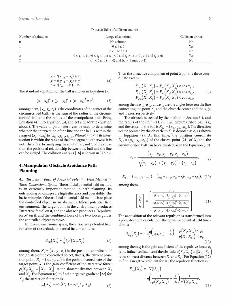
�e corresponding ´ow chart is shown in Figure 1:
(7) If ���(��) < ���(��), update the contemporary optimal solution ��← ��, ��← ��. Otherwise ��← ��,��← ��.
(8) If � >� − g, output the global optimal solution �� = (�1, �2, �3), and end. Otherwise, return to step (5).
(9) At this time, the angle of each joint angle of the arm is � = [ �(1) + �1 �(2) + �2 �(3) + �3 0 0 0 ], so that the corresponding end position �� can be obtained according to the kinematics of the manipu-lator, that is, the process of completing the small dis-placement of the end of the manipulator.
�e process of changing the direction of motion using the RRT algorithm is as follows:
(1) Start with the current position of the end of the manipulator and record it as �start. Given the separa-tion distance Δ�.
(2) A random point �rand is generated in the working space of the manipulator.
(3) Find the node �near closest to �rand in the RRT and calculate the Euclidean distance � from �near to �rand. If � < Δ�, the new node �new is equal to �rand. Otherwise, �new is equal to the point a§er �new extends Δ� in the direction of �rand.
(4) Determine whether the space segment of �near to �new collides with an obstacle. If it collides, round o� �new and return to step (2). Otherwise, add �new to the tree.
(5) Determine whether the maximum number of itera-tions has been reached. If not, return to step (2) to continue the loop. Otherwise, draw the path and mark the node at the end of the path as the virtual target point, denoted as �ggg.
(6) �e direction in which �start points to �ggg is taken as the next action direction of the manipulator.
In the commonly used path planning method [16], the virtual target point method is also used to jump out of the local extremum. Its process is to create a virtual target point near the end, a§er the end needs to reach the virtual target point, and then move to the �nal target point. In contrast, the method in this paper only changes the direction of the action through the randomly generated virtual target point, and does not need to arrive, that is, a§er running one step, the virtual target point disappears instantly. �is can improve work e¡ciency and ensure path quality.
In general, the random principle of dynamic virtual target points reduces the likelihood that the manipulator will fall into local extremum. �e dynamic virtual target point and the appropriate in´uence distance make it di¡cult for the end of the manipulator to reach a dangerous area that is too close to the obstacle, which improves the obstacle prediction ability of the manipulator to some extent. �e invisible obstacle treat-ment better overcomes the problem of the structural structure of the manipulator. Setting the extreme point jump-out func-tion solves the stagnation and oscillation of the manipulator.
Journal of Robotics6
�at is, Δ��(��, ��−1) is the distance between two points ��and ��−1. �0 is the starting position coordinate. �erefore, the end moving distance during the entire movement is approximately:
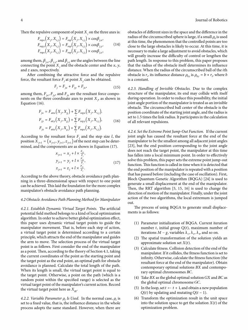
5.1. Simulation Experiment of Single Obstacle Path Planning. Let the coordinates of the target point be �g0 = (0.3500, −0.2500, 0.4000), and calculate the spherical center coordinates and radius of the obstacle according to the established obstacle model as ��� = (0.4000, −0.3000, −0.1500)and � = (0.2500), respectively. According to the ´ow chart of the obstacle avoidance path planning of the manipulator, the simulation results are shown in Figures 2 and 3.
It can be seen from the Figure 2 that the manipulator avoids the obstacle and accurately reaches the vicinity of the target point, forming a relatively smooth path. It can be seen
(21)Δ�sum = Δ�1 + Δ�2 + ⋅ ⋅ ⋅ + Δ��sum .
5. Simulation Experiment
In order to verify the e�ectiveness of the path planning method proposed in this paper, simulation experiments were carried out with Matlab R2016b. �e simulation experiment is from single obstacle to multi-obstacle, and compared with the sim-ulation results of common methods. �e initialization of the parameters is shown in Table 3.
Record the total number of steps required for the manip-ulator to complete the task as �
sum. During the movement, the
angle changes of the three joints are respectively recorded as Δ�1,�, Δ�2,�, and Δ�3,�, where � = 1, 2, . . . , �sum, then their cumu-lative angle changes are:
�erefore, the cumulative angle change of the entire manipu-lator is:
During the movement, the coordinate value of the end posi-tion of the manipulator is recorded as �� (� = 1, 2, . . . , �sum), and the change of the end position is as follows:
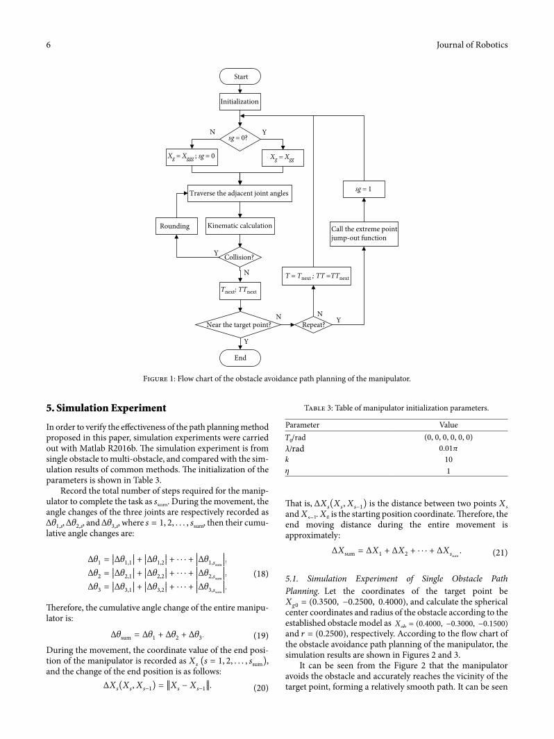
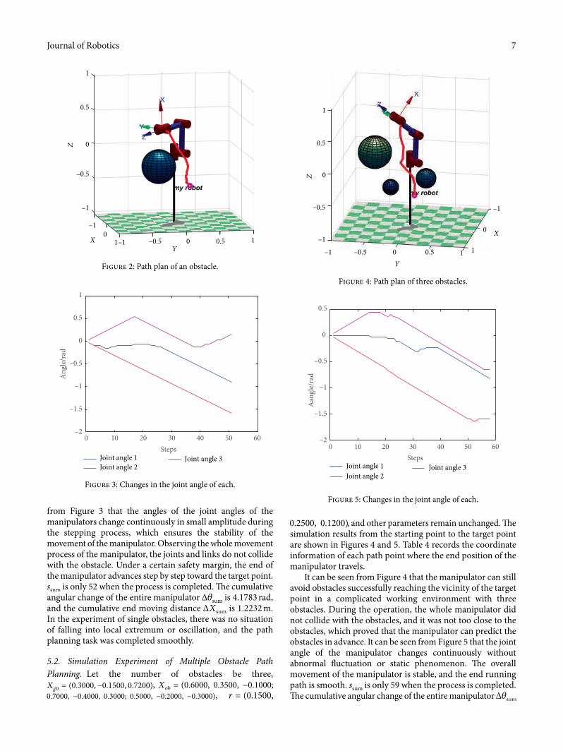
0.2500, 0.1200), and other parameters remain unchanged. �e simulation results from the starting point to the target point are shown in Figures 4 and 5. Table 4 records the coordinate information of each path point where the end position of the manipulator travels.
It can be seen from Figure 4 that the manipulator can still avoid obstacles successfully reaching the vicinity of the target point in a complicated working environment with three obstacles. During the operation, the whole manipulator did not collide with the obstacles, and it was not too close to the obstacles, which proved that the manipulator can predict the obstacles in advance. It can be seen from Figure 5 that the joint angle of the manipulator changes continuously without abnormal ´uctuation or static phenomenon. �e overall movement of the manipulator is stable, and the end running path is smooth. �sum is only 59 when the process is completed. �e cumulative angular change of the entire manipulator Δ�sum
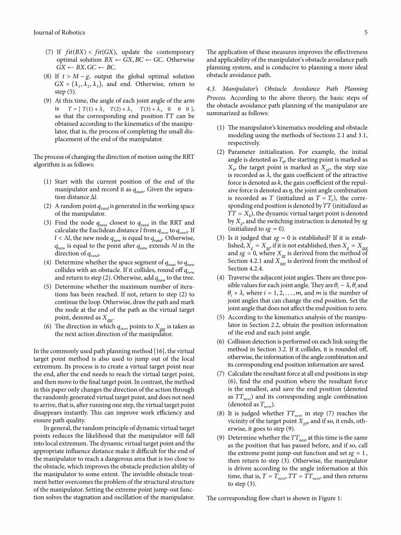
from Figure 3 that the angles of the joint angles of the manipulators change continuously in small amplitude during the stepping process, which ensures the stability of the movement of the manipulator. Observing the whole movement process of the manipulator, the joints and links do not collide with the obstacle. Under a certain safety margin, the end of the manipulator advances step by step toward the target point. �sum is only 52 when the process is completed. �e cumulative angular change of the entire manipulator Δ�sum is 4.1783 rad, and the cumulative end moving distance Δ�sum is 1.2232 m. In the experiment of single obstacles, there was no situation of falling into local extremum or oscillation, and the path planning task was completed smoothly.
5.2. Simulation Experiment of Multiple Obstacle Path Planning. Let the number of obstacles be three, �g0 = (0.3000,−0.1500, 0.7200), ��� = (0.6000, 0.3500, −0.1000;0.7000, −0.4000, 0.3000; 0.5000, −0.2000, −0.3000), � = (0.1500,
1
0.5
–0.5
0
–1
–1
1–1 –0.5 0 0.5 1
Z
XY
0
Figure 2: Path plan of an obstacle.
0 10 20 30 40 50 60Steps
–2
–1.5
–1
–0.5
0
0.5
1
Ang
le/r
ad
Joint angle 1Joint angle 2
Joint angle 3
Figure 3: Changes in the joint angle of each.
0 10 20 30 40 50 60Steps
–2
–1.5
–1
–0.5
0
0.5A
angl
e/ra
d
Joint angle 1Joint angle 2
Joint angle 3
Figure 5: Changes in the joint angle of each.
1
0.5
0Z
Y
X
–0.5
–1
–1 0 0.5 1
–1
0
1–0.5
Figure 4: Path plan of three obstacles.
Journal of Robotics8
adjustments, the arm jumped out of the local extremes that were trapped. �e reason why the repeated position information does not appear in the process is because the adjusted information covers the repeated information when the extreme point jump-out function adjusts the manipulator. In this way, the manipulator will not stop moving during the whole operation. In this operation, the manipulator not only e�ectively addresses the extreme point and oscillation problems but also ensures the path quality as much as possible. Eventually, the manipulator runs stably along a more desirable path to the vicinity of the target point.
is 4.2158 rad, and the cumulative end moving distance Δ�sumis 1.4400 m. Observing the coordinate information of each path point at the end of the manipulator in Table 4, the end position information is di�erent. However, when observing the running process of the program, it was found that the manipulator had a phenomenon of repeating with the previous position in the 21th step and the 24th step, that is, the manipulator was caught in the local extreme value. A§er this happens, the main program calls the extreme point jump-out function twice, and adjusts the position of the end of the manipulator and its action direction in time. A§er only two
Table 6: Comparison of data between two planning methods for two obstacles.
�e corresponding histogram is shown in Figures 9–11, where the graph reaching the maximum represents Δ�sum.
commonly used method for manipulator obstacle avoidance path planning. �e disadvantage of using this method is that because the target point is �xed, the manipulator is more likely to fall into local extremum, and the path quality cannot be guaranteed during the process of jumping out of the local extremum. In order to further prove the e�ectiveness and superiority of the method in this paper, the following comparative experiments under the same conditions were carried out. �e comparison data of the six groups are shown in Tables 5–7. Among them, the data results obtained by the method of this article are placed outside “()”, the data results obtained by the commonly used method are placed inside “()”, and ∞ indicates that the planning fails.
It can be obtained from Table 5 (Figures 6–8) that in the case of an obstacle, the di�erence between the two methods is not large, and the path planning task can be completed well. However, it can be seen from the Table 6 (Figures 9–11) of the two obstacles that the probability of occurrence of extreme points in the commonly used methods begins to increase, and even the phenomenon of planning failure occurs. From the simulation data of three or more obstacles shown in Table 7 (Figures 12–14), when the environment is more complicated, the improved method proposed in this paper shows a big advantage in terms of the number of steps, the cumulative angle change, and the cumulative end moving distance. From the comprehensive analysis of the data in Tables 5–7, it can be seen that when the improved obstacle avoidance path planning method is applied, the manipulator can complete the task with fewer steps, and the overall angle change is small, and the end moving distance is obviously shortened. �e success rate of path planning has also increased signi�cantly. It can be calculated that the improved method proposed in this paper reduces the possibility of the manipulator falling into the extreme point by about 27.78%, and reduces the possibility of planning failure by about 22.22%. Observe the relevant simulation results of two or more obstacles and analyze the data that both methods are planned successfully. It can be obtained that compared with the
5.3. Comparison with Commonly Used Path Planning Methods. Literatures [15, 16] use the hybrid algorithm of arti�cial potential �eld method and RRT algorithm to realize the obstacle avoidance path planning of the manipulator. �e main idea of the method is as follows: the arti�cial potential �eld method is used for path planning; when the manipulator is trapped in the local extremum, the RRT algorithm is used to establish the virtual target point to jump out of the local extremum; when the manipulator jumps out of the local extremum, the arti�cial potential �eld method continues to be used for path planning. �is method is common in the existing literature. �erefore, this paper refers to it as the
1.2
1.3
1.4
1.5
1.6
1.7
1.8
1 2 3 4 5 6Serial number
Data outside ()Data in ()
Cum
ulat
ive
end
mov
ing
dist
ance
Figure 8: A comparison chart of Δ�sum
when there is an obstacle.
40
42
44
46
48
50
52
54
56
58
60
1 2 3 4 5 6Serial number
Data outside ()Data in ()
�e t
otal
num
ber o
f ste
ps
Figure 6: A comparison chart of �sum
when there is an obstacle.
3
3.2
3.4
3.6
3.8
4
4.2
4.4
4.6
4.8
1 2 3 4 5 6Serial number
Cum
ulat
ive
angl
e ch
ange
s
Data outside ()Data in ()
Figure 7: A comparison chart of Δ�sum
when there is an obstacle.
Journal of Robotics10
with complex working environment, the system still has the advantages of smooth running of the manipulator, continuous change of joint angle, less control steps, smaller cumulative angle change, and shorter cumulative end moving distance. It improves the success rate of path planning and also ensures path quality. �e improved method proposed in this paper solves the problem of obstacle avoidance path planning of mechanical arm in three-dimensional space, which provides reference for manip-ulator control in saving energy and �nding optimized path.
commonly used method, the improved method of this paper reduces the planned step number by about 27.37%, reduces the cumulative angle change by about 31.66%, and shortens the cumulative end moving distance by about 28.77%, which fully re´ects the e�ectiveness and superiority of the method.
6. Summary
Aiming at the problems existing in the commonly used path planning methods, this paper establishes a relatively complete mechanical arm obstacle avoidance path planning system by adopting a series of improvement measures such as establishing dynamic virtual target points and setting extreme point jump-out functions. �e simulation results show that when dealing
1.1
1.4
1.7
2
2.3
2.6
2.9
3.2
1 2 3 4 5 6Serial number
Data outside ()Data in ()
Cum
ulat
ive
and
mov
ing
dist
ance
Figure 11: A comparison chart of Δ�sum
when there are two obstacles.
2
4
6
8
10
12
14
16
1 2 3 4 5 6Serial number
Data outside ()Data in ()
Cum
ulat
ive
angl
e ch
ange
s
Figure 10: A comparison chart of Δ�sum
when there are two obstacles.60
80
100
120
140
160
180
200
220
1 2 3 4 5 6Serial number
Data outside ()Data in ()
�e
tota
l num
ber o
f ste
ps
Figure 12: A comparison chart of �sum
when there are 3 or more obstacles.
40
60
80
100
120
140
160
180
1 2 3 4 5 6Serial number
Data outside ()Data in ()
�e t
otal
num
ber o
f ste
ps
Figure 9: A comparison chart of �sum
when there are two obstacles.
11Journal of Robotics
Supplementary Materials
�e source program used to support the �ndings of this study is included within the supplementary information �le. (Supplementary Materials)
References
[1] M. W. Spong, S. Hutchinson, and M. Vidyasagar, Robot Modeling and Control, China Machine Press, Beijing, 2016.
[2] D. F. Zhang, H. Zhao, L. Xu, M. L. Liu, and J. Zhang, “Research on workspace analytic method of improved grid method based on industriaI robotic arm,” Manufacturing Automation, vol. 41, no. 4, pp. 69–70+90, 2019.
[3] P. Lozano and T. Rez, “Spatial planning: a con�guration space approach,” IEEE Transaction on Computers, vol. 32, no. 2, pp. 108–120, 1983.
[4] P. Lozano and T. Rez, “A simple motion-planning algorithm for general robot manipulator,” IEEE Journal of roboties and Automation, vol. 3, no. 3, pp. 224–238, 1987.
[5] S. M. Lavalle, “Rapidly-exploring random trees: a new tool for path planning,” Algorithmic & Computational Robotics New Direction, pp. 293–308, 1998.
[6] L. Kavraki, P. Svestka, J. Latommbe, and M. Overmars, “Probabilistic roadmaps for path planning in high-dimensional con�guration spaces,” IEEE Transactions on Robotics & Automation, vol. 12, no. 4, pp. 566–580, 1994.
[7] X. C. Chen and J. Huang, “Collision free path planning of robot manipulator based on arti�cial potential �eld and quantum-based particle swarm optimization,” in Proceedings of the 36th Chinese Control Conference, pp. 26–28, Dalian, China, 2017.
[8] Y. Dai and M. Zhao, “Manipulator path-planning avoiding obstacle based on screw theory and colony algorithm,” Journal of Computational and �eoretical Nanoscience, vol. 13, pp. 922–927, 2016.
[9] Y. Tan, “Robotic arm trajectory planning method by inserting optimal intermediate point searched by improved genetic algorithm,” Manufacturing Technology & Machine Tool, vol. 5, pp. 139–143+148, 2019.
[10] O. Khatib, “Real-time obstacle avoidance for manipulators and mobile robots,” in IEEE International Conference on Robotics and Automation, pp. 90–98, St. Louis, MO, 2003.
[11] L. Xie and S. Liu, “Dynamic obstacle-avoiding motion planning for manipulator based on improved arti�cial potential �led,” Control �eory & Applications, vol. 35, no. 9, pp. 1239–1249, 2018.
[12] S. K. Wang, L. Zhu, and J. Z. Wang, “Six-degree-of-freedom mechanical arm obstacle avoidance path planning based on navigation potential function method,” Transactions of Beijing Institute of Technology, vol. 35, no. 2, pp. 186–191, 2015.
[13] J. L. Wang, G. L. Zhang, F. Yang, and B. Jing, “Improved arti�cial �eld method on obstacle avoidance path planning for manipulator,” Computer Engineering and Applications, vol. 49, no. 21, pp. 266–270, 2013.
[14] W. Ji, F. Y. Cheng, D. A. Zhao, Y. Tao, S. Ding, and J. D. Lü, “Obstacle avoidance method of apple harvesting robot manipulator,” Transactions of �e Chinese Society of Agricultural Machinery, vol. 44, no. 11, pp. 253–259, 2013.
[15] Z. C. He, Y. L. He, and B. Zeng, “Obstacle avoidance path planning for robot arm based on mixed algorithm of arti�cial
Data Availability
�e data used to support the �ndings of this study are included within the article. �e source program used to support the �ndings of this study is included within the supplementary information �le.
Conflicts of Interest
�e authors declare that they have no con´icts of interest.
potential �eld method and RRT,” Industrial Engineering Journal, vol. 20, no. 2, pp. 56–63, 2017.
[16] J. Zhu and M. Y. Yang, “Path planning of manipulator to avoid obstacle based on improved arti�cial potential �eld method,” Computer Measurement & Control, vol. 26, no. 10, pp. 205–210, 2018.
[17] Z. X. Cai, Robotics Foundation, Mechanical Industry Press, China, 2015.
[18] B. Q. Tian, J. C. Yu, and A. Q. Zhang, “Dynamic modeling of wave driven unmanned surface vehicle in longitudinal pro�le based on D-H approach,” Journal of Central South University, vol. 22, no. 12, pp. 4578–4584, 2015.
[19] H. M. C. M. Herath, R. A. R. C. Gopura, and T. D. Lalitharatne, “An underactuated linkage �nger mechanism for hand prostheses,” Modern Mechanical Engineering, vol. 8, no. 2, pp. 121–139, 2018.
[20] X. Q. Lv and M. Zhao, “Application of improved BQGA in robot kinematics inverse solution,” Journal of Robotics, vol. 2019, Article ID 1659180, p. 7, 2019.
[21] Y. Peng, W. Q. Guo, M. Liu, J. X. Cui, and S. R. Xie, “Obstacle avoidance planning based on arti�cial potential �eld optimized by point of tangency in three-dimensional space,” Journal of System Simulation, vol. 26, no. 8, pp. 1758–1762+1768, 2014.
[22] L. Z. Chen and B. Q. Yu, Mechanical Optimization Design Method, Metallurgical Industry Press, Beijing, 2014.
[23] P. Y. Ma, Research on Obstacle Avoidance Path Planning of Six-Degree-of-Freedom Mechanical Arm, South China University of Technology, China, 2010.
[24] S. Y. Li and P. C. Li, Quantum Computation and Quantum Optimization Algorithm, Harbin Institute of Technology Press, Harbin, 2009.