Hindawi Publishing CorporationMathematical Problems in EngineeringVolume 2013 Article ID 676148 9 pageshttpdxdoiorg1011552013676148
Research ArticlePricing Options and Convertible Bonds Based onan Actuarial Approach
Jian Liu12 Lizhao Yan3 and Chaoqun Ma1
1 Business School Hunan University Changsha 410082 China2 School of Economics and Management Changsha University of Science and Technology Changsha 410004 China3Hunan Normal University Press Changsha 410081 China
Correspondence should be addressed to Chaoqun Ma cqmahnucn
Received 2 September 2013 Accepted 19 October 2013
Academic Editor Fenghua Wen
Copyright copy 2013 Jian Liu et al This is an open access article distributed under the Creative Commons Attribution License whichpermits unrestricted use distribution and reproduction in any medium provided the original work is properly cited
This paper discusses the pricing problem of European options and convertible bonds using an actuarial approach We get thepricing formula of European options extend the pricing results to the case with continuous dividend and then derive the call-putparity relation Furthermore we get the general expression of convertible bond price Finally we conduct a comparative analysis ofnumerical simulation and make an empirical analysis between the B-S model and the actuarial model using the actual data in theChinese stock market The empirical results show that the efficiency of the actuarial model is superior to the B-S model
1 Introduction
The contingent claim pricing has always been one of thecore subjects in the field of financial engineering researchTo price contingent claims correctly and scientifically is thebasis of financial risk management as well as an indispens-able component of modern finance Black and Scholes [1]derived the well-known Black-Scholes (B-S) formula usingarbitrage reasoning and stochastic analysis in their classicpaper on option pricing and thus established the optionpricing theory The B-S pricing model has had a hugeinfluence on the financial theory However it was basedon multiple assumptions such as a normal distributionfor the underlying asset price process no divided payingfor the underlying asset and the constant risk-free interestrate which apparently do not fit in with the ever-changingfinancial market Later a number of researchers improvedand popularized the B-S model Merton [2] validated theB-S formula using the arbitrage theory and derived theanalytic solution to the continuous time model for optimalconsumption and investment decision using dynamic pro-gramming methods Cox et al [3] proposed the binominaloption pricing model Duffie [4] made further inferencefor the B-S formula with the conventional option pricing
approach Liu and Zhao [5] develop an efficient latticeapproach for option pricing Ammann et al [6] proposeand empirically investigate a pricing model for convertiblebonds based on the enhancedMonte Carlo simulation Xu [7]uses a lattice approach to pricing the convertible bond assetswap
Most of the existent research on option pricing was basedon martingale measure or numerical simulation theory inthe framework of Black-Scholes option pricing approach andis only applicable in a complete financial market where allcontingent claims are capable of being replicated accuratelywith the asset portfolios available on the existent financialmarkets that is to say the market is in an equilibriumarbitrage-free and one and only equivalent martingale mea-sure exists But the complete market assumption may not beperfectly relevant to the actual investment environment If thefinancial market is incomplete assets cannot be accuratelyreplicated or hedged like in a complete market A commonalternative practice is to seek a family of final wealth derivedfrom self-financing strategies to approach the value of theasset which naturally entails errors For example Follmerand Sondermann [8] proposed the ldquomean-variancerdquo criterionto measure the error but the solution process is rathercomplicated
2 Mathematical Problems in Engineering
Bladt and Rydberg [9] first proposed an actuarialapproach to pricing options which transforms the optionpricing into a problem equivalent to determining thefair insurance premium As no economic assumptions areinvolved this approach is valid for incomplete markets aswell as for completemarkets and demonstrated that the pricederivedwhereby is consistent with that from the B-Smodel inthe continuous time case Yan and Liu [10] used the actuarialapproach to derive the European option pricing formulawhere the stock price is assumed to follow the Ornstein-Uhlenbeck (O-U) process and Zhao and He [11] studiedthe option pricing model where the stock price is assumedto follow a fractional O-U process in a risk neutral marketThe assumption of the stock price following the O-U processavoids the limitation that the stock price tends to change inone direction under the lognormal distribution assumptionand weakens the tendency of the stock price rise But theassumption for the above model that the interest rate is adeterministic function of time cannot satisfy the requirementof the actual conditions of themarket A number of empiricallines of evidence show that in real financial markets theinterest rate has the property of mean-reversion the volatilityof the long-term interest rate is less than that of the short-terminterest rate and the volatility is greater when the interestrate is relatively higher [12 13] Liu et al [14] studied thereload stock option pricing under the assumption of theinterest rate following the Hull-White model with martingalepricing method The stochastic interest rate model assumesthat the interest rate converges with the time at a certainmeanreversion level
The content of this paper is arranged as follows InSection 2 we make some basic assumption for the financialmarket where the stock prices are driven by O-U processand the interest rates are driven by Hull-White model InSection 3 we consider themodels in the continuous time andapply the actuarial approach to price the European optionand the convertible bond To show the role that the actuarialapproach and the stochastic interest rates play we conduct acomparative analysis of numerical simulation in Section 4 Asin Section 5 we make an empirical analysis between the B-Smodel and the actuarial model using the actual data in theChinese stock market Section 6 concludes the paper
2 Basic Assumption
Suppose that the financial market is frictionless and contin-uous and there are two assets The risky asset is the stockand the risk-free asset is the bond A complete probabilityspace (Ω 119865 119865
119905119905ge0 119875) describes the financial market where
the filtration satisfies the usual conditionsAssume that the stock price 119878(119905) follows the Ornstein-
where the parameters 119886(119905) 119887(119905) and 120590119903(119905) are some deter-
minate functions of time 119905 The Hull-White model is themean-reversionmodel where the parameter 119886(119905) is the long-term average level and 119887(119905) is the average reversion rate ofinterest rates When the parameters 119886(119905) and 119887(119905) are con-stant the Hull-White model (2) becomes the Vasicek modelThe stochastic processes 119861(119905) 119905 ge 0 and 119882(119905) 119905 ge 0 aretwo standard Brownian Motions in the defined probabilityspace (Ω 119865 119865
119905119905ge0 119875) and their correlation coefficient is
supposed to be 120588Now we give two definitions of the actuarial approach
Definition 1 (see [9]) The expected yield rate of the stockprice process 119878(119905) 0 le 119905 le 119879 in the time interval [0 119879] isdefined by int119879
0120573(119905)119889119905 which satisfies the following equation
119890int119879
0120573(119905)119889119905
=119864 [119878 (119879)]
119878 (3)
Definition 2 (see [9]) Suppose the expiration date of theEuropean option is119879 and the strike price is119870 In the actuarialapproach the stock price is discounted by the expected yieldrate defined in (3) and the strike price is discounted bythe riskless interest rate on maturity The European optionvalue is defined as the expectation of the difference whichis between the two discount values on the actual probabilitymeasure as the option is exercised The sufficient and neces-sary condition for exercising the European call option on 119879is
Let 119862(119870 119879) denote the call value and 119875(119870 119879) denote the putvalue at the time 0 Then in the actuarial approach the twooptions values are defined as follows respectively
In this section we firstly consider the pricing problem of theEuropean options in the financial market models describedaboveThenwe extend the pricing result to the options whoseunderlying asset has continuous dividend and derive the call-put parity relation using the actuarial approach Furthermorewe get the general expression of convertible bond price Atfirst we offer two important lemmas
Lemma 3 (see [15]) If the random variables 1198821and 119882
2are
both standard normally distributed with mean 0 and variance1 notated as119873(0 1) and their covariance is Cov(119882
11198822) = 120588
then for any real numbers 119886 119887 119888119889 and 119896 one has the followingequation
119864 [1198901198881198821+11988911988221
1198861198821+1198871198822ge119896]
= 119890(12)(119888
2+1198892+2120588119888119889)
119873(119886119888 + 119887119889 + 120588 (119886119889 + 119887119888) minus 119896
radic1198862 + 1198872 + 2120588119886119887
)
(7)
Lemma 4 If the stock price S(t) is driven by the O-U process(1) then one gets the following equations
31 European Options Pricing We consider the Europeanoptions call and put whose underlying assets are stocksSuppose that the exercise date of the options is 119879 and thestrike price is 119870
Theorem 5 Assume that the short-term interest rate isdescribed by the Hull-White model and the stock process 119878(119905)119905 ge 0 follows the O-U process then at the time 0 the pricingformulas of the call and put are as follows respectively
119862 (119870 119879) = 119878119873 (1198891) minus 119870 exp 1
119862 (119870 119879) = 119878119873 (1198891) minus 119870 exp 1
21205902
119883minus 119866 (0 119879)119873 (119889
2)
(23)
Similarly we get the value of put option as follows
119875 (119870 119879) = 119870 exp 121205902
119883minus 119866 (0 119879)119873 (minus119889
2) minus 119878119873 (minus119889
1)
(24)
Furthermore we deduce the following pricing inferences
Inference 1 Suppose that the stock process 119878(119905) 119905 ge 0 fol-lows the O-U process (1) and the interest rate is describedby the Hull-White model (2) then the call-put parity of theEuropean options in the actuarial approach is
Inference 2 Under the market models (1) and (2) the under-lying stock has continuous dividend yield marked by 119902(119905)Then respectively the pricing formulas of the call and putoption in the actuarial approach at time 0 are
1=ln (119878119870) + 119866 (0 119879) minus int119879
0119902 (119905) 119889119905 + (12) 120590
2
119884+ 120588120590119883120590119884
radic1205902119883+ 1205902119884+ 2120588120590
119883120590119884
1198891015840
2= (ln( 119878
119870) + 119866 (0 119879) minus int
119879
0
119902 (119905) 119889119905
minus 1205902
119883minus1
21205902
119884+ 120588120590119883120590119884)
times (radic1205902119883+ 1205902119884+ 2120588120590
119883120590119884)minus1
(27)
32 Convertible Bond Pricing We consider the pricing prob-lem of convertible bond with the call provision It is based onthe actuarial approach where the stock price is driven by O-U process and the interest rate followsHull-Whitemodel Forthe callable convertible bonds based on the classical theoryof optimal investment strategy Brennan and Schwartz [16]
and Ingersoll [17] the investors will not exercise the rightof conversion while the issuers will immediately exercise theright of redemption when the stock prices reach the callableprice for the first time [18] Let 119879 be the maturity date of theconvertible bond and let 120591lowast be the first time when the stockprice goes up to the callable trigger price then the optimalexercise time 120591 = 120591lowast otherwise 120591 = 119879
Theorem 6 Suppose that the face value of the convertiblebond is 119861
119865 the conversion price is 119870
1 and the callable trigger
price is 1198702 then the general expression of convertible bond
price 119867 is given by
119867 = E [119890minusint120591lowast
0120573(119905)119889119905
times (1198702
119861119865
1198701
+ 119888 (120591lowast)) times 1
120591lowastle119879]
+ [119861119865
1198701
119878119873 (1198893) + 119888 (119879) exp 1
21205902
119883minus 119866 (0 119879)119873 (119889
4)]
times 119875 (120591lowastgt 119879)
+ [(119861119865+ 119888 (119879)) sdot exp 1
21205902
119883minus 119866 (0 119879)119873 (minus119889
4)]
times 119875 (120591lowastgt 119879)
(28)
where
1198893=ln (119878119870
1) + 119866 (0 119879) + (12) 120590
2
119884+ 120588120590119883120590119884
radic1205902119883+ 1205902119884+ 2120588120590
119883120590119884
1198894=ln (119878119870
1) + 119866 (0 119879) minus 120590
2
119883minus (12) 120590
2
119884+ 120588120590119883120590119884
radic1205902119883+ 1205902119884+ 2120588120590
119883120590119884
(29)
Proof As 120591lowast is the first time when the stock price goes up tothe callable trigger price so 120591lowast = inf119905 119878
119905ge 1198702 Under the
optimal investment strategy the optimal execution time 120591 is
120591 = 120591lowast trigger before the expiry119879 no trigger before the expiry
(30)
Let 119888(119905) express the time 119905 present value of the interestincome before 119905 then the theoretical value of the convertiblebond at the time 120591 defined by 119892(119903 119878 120591) is given by
119892 (119903 119878 120591) =
119861119865
1198701
1198702+ 119888 (120591lowast) 120591lowast le 119879
Then the general expression of convertible bond pricesatisfies (28) Sowith (28) we can obtain the convertible bondprice using the Monte Carlo simulation
4 Numerical Examples
The general European options mainly take the classic B-S formula results as the reference prices However thereare usually some differences between the actual transactionprices and the reference prices of the options and it is difficultto obtain the data of the actual option prices Therefore wefirst consider some specific numerical examples under givenparameters to compare the results of the actuarial pricingformula with the B-S formula and to reveal the impact ofthe stochastic interest rates on pricing results when the stockprices followO-U process Here it should be pointed out thatif there is no arbitrage in themarket theremust be at least onerisk-neutral martingale measure and the stock price processcan be transformed into a martingale In this case the O-Umodel is free of arbitrage just as the method of B-S model is
Now we make numerical examples to the Europeanoptions The parameters in the financial market models areselected as follows
119870 = 60 119879 = 1 119886 = 0034
119887 = 0016 120590119904= 0395 120590
119903= 0023
120572 = 02 119903 = 00245 120588 = minus058
(35)
and we obtain the option pricing results by MatlabAs the underlying stock prices followO-Uprocess and the
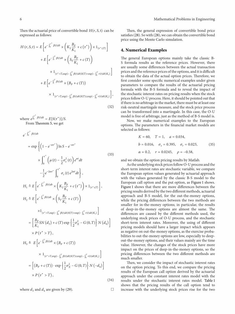
short-term interest rates are stochastic variable we comparethe European option values generated by actuarial approachwith the values generated by the classic B-S model to theEuropean call option and the put option as Figure 1 showsFigure 1 shows that there are more differences between thepricing results derived by the two differentmethods actuarialapproach and B-S model for the out-the-money optionswhile the pricing differences between the two methods aresmaller for in-the-money options in particular the resultsof deep-in-the-money options are almost the same Thedifferences are caused by the different methods used theunderlying stock prices of O-U process and the stochasticshort-term interest rates Moreover the using of differentpricing models should have a larger impact which appearsas negative on out-the-money options as the exercise proba-bilities to out-the-money options are low especially to deep-out-the-money options and their values mainly are the timevalue However the changes of the stock prices have moreimpact on the prices of deep-in-the-money options so thepricing differences between the two different methods aremuch smaller
Then we consider the impact of stochastic interest rateson the option pricing To this end we compare the pricingresults of the European call option derived by the actuarialapproach under the constant interest rates model with theresults under the stochastic interest rates model Table 1shows that the pricing results of the call option tend toincrease with the underlying stock prices rise for the two
Mathematical Problems in Engineering 7
ActuarialB-S
45
40
35
30
25
20
15
10
5
00 10 20 30 40 50 60 70 80 90 100
Stock price
Call
optio
n
(a)
ActuarialB-S
60
50
40
30
20
10
00 10 20 30 40 50 60 70 80 90 100
Stock price
Put o
ptio
n
(b)
Figure 1 Comparison of the options values from actuarial approach under stochastic interest rates and O-U process with those from B-Sformula
Table 1 Comparison of the results given by the actuarial approachwith stochastic interest rates and constant interest rates
different models However if the underlying stock price isfixed the pricing result of the call under constant stochasticinterest rates is lower than the pricing result under stochasticinterest rates And with the stock price increasing thedifference between the two models increases at first andthen decreases The stochastic interest rates increase theuncertainty and may increase the prices of the call option
5 Empirical Study
51 Data and Parameters We analyze the differences of thetwo models B-S model and actuarial model using the actualdata in the Chinese stock market However there are onlythree warrants that are similar to the call option The onlydifference between the warrant and the option is that theoption is a standardized contract but the warrant is notHowever it would not affect the results Sowe choose the dataof Changhong CWB1 which is equivalent to a European calloption as its exercise ratio is 1 1 and the underlying stock hasnot paid dividend during the chosen period thenwe need notadjust the prices of the stock and the warrantThe data coversthe period fromAugust 19 2009 when theChanghongCWB1was listed toMay 20 2010 and the time interval between eachobservation is one day This means that we end up with 181
observations and this is the longest sample available to usThe data are taken from the Shanghai Stock Exchange andare collected through the Dazhihui quote software
Next we need to estimate the parameters in the modelsSome parameters we can get from public information are asfollows the strike price of the Changhong CWB1 is119870 = 523the exercise date is 119879 = 2 years the interval is Δ119905 = 1250and the interest rate at 0 time is 119903 = 00225 which is theofficial interest rate for one-year deposits during the period2009-2010 As for the parameters in the interest rate modelwe use the daily data of 7-day repo rates in the ShanghaiStock Exchange from August 19 2009 to May 20 2010 andthe MLE method to estimate the parameters by Matlab Theresult shows that the estimated parameters of the short-term interest rates driven by the Hull-White model in Chinamarket are 119886 = 00322 119887 = 01937 and 120590
119903= 00863 In
order to estimate the parameters of the underlying stock weuse the historical data of Changhong shares during the sametime to compute the results 120590
119878= 06968 and 120572 = 01359 by
the MLE method A large number of works in the literaturehave revealed that the correlation of the stock price and theinterest rate is weak negative [19] and we indeed get theparameter 120588 = minus0284 during the chosen time
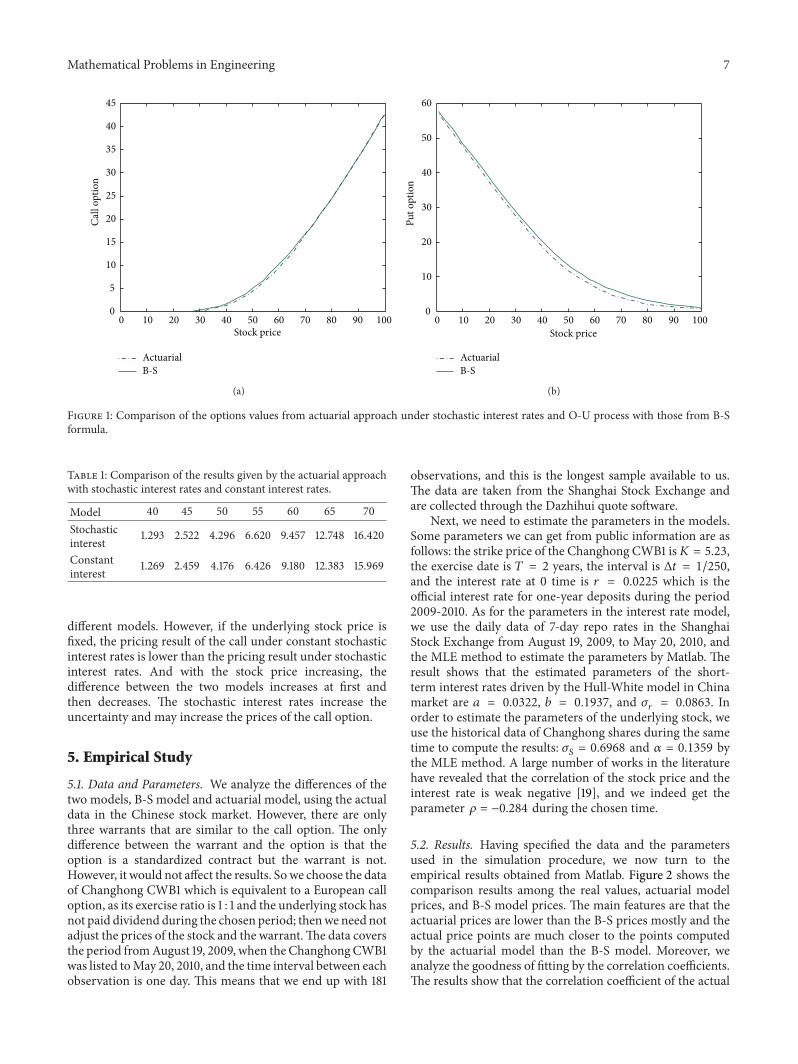
52 Results Having specified the data and the parametersused in the simulation procedure we now turn to theempirical results obtained from Matlab Figure 2 shows thecomparison results among the real values actuarial modelprices and B-S model prices The main features are that theactuarial prices are lower than the B-S prices mostly and theactual price points are much closer to the points computedby the actuarial model than the B-S model Moreover weanalyze the goodness of fitting by the correlation coefficientsThe results show that the correlation coefficient of the actual
8 Mathematical Problems in Engineering
4
35
3
25
2
15
1
Chan
ghon
g CW
B1
4 45 5 55 6 65 7 75 8Stock price
ActuarialB-SActual price
Figure 2 Comparison of the values among the actual data actuarialmodel and B-S model
prices and the actuarial model prices is 09652 and thecorrelation coefficiency of the actual prices and the B-Smodelprices is 09607which is lower than the former It is an explicitevidence that the efficient of the actuarialmodel is superior tothe B-S modelThe analysis also shows that the correlation ofthe actuarial prices and the B-S prices is strong and positiveas their correlation coefficient is 09996
6 Conclusions
In the martingale pricing method the prices of the financialderivative securities (or contingent claims) are obtained bydiscounting their expectations of future cash flows which arecomputed with risk neutrality It is valid for the completemarket because the unique equivalent martingale existsHowever if the market is not arbitrage-free and incompletethe equivalent martingale measure does not exist or existsbut is not unique then it is hard to price by the martingalepricing method As no economic assumptions are involvedthe actuarial approach is valid for incomplete markets as wellas for complete markets and needs not find an equivalentmartingale measure for pricing This paper discusses thepricing problem of the European options and convertiblebonds using the actuarial approach We get the pricingformula of the European options extend the pricing resultsto the case with continuous dividend and then derive thecall-put parity relation Furthermore we get the generalexpression of convertible bond price Finally we conduct acomparative analysis of numerical simulation and make anempirical analysis between the B-S model and the actuarialmodel using the actual data in the Chinese stock marketTheempirical results show that the efficiency of actuarial modelis superior to the B-S model
Acknowledgments
The authors would like to express gratitude for the supportgiven by the National Natural Science Foundation of China
(no 71201013) the National Natural Science InnovationResearch Group of China (no 71221001) the National Sci-ence Fund for Distinguished Young Scholars of China (no70825006) and the Humanities and Social Sciences Projectof the Ministry of Education of China (no 12YJC630118)
References
[1] F Black and M Scholes ldquoThe pricing of options and corporateliabilitiesrdquo Journal of Political Economy vol 81 no 3 pp 637ndash654 1973
[2] R C Merton ldquoTheory of rational option pricingrdquo Bell Journalof Economics and Management Science vol 4 no 1 pp 141ndash1831973
[3] J C Cox S A Ross and M Rubinstein ldquoOption pricing asimplified approachrdquo Journal of Financial Economics vol 7 no3 pp 229ndash263 1979
[4] D Duffie Security Markets Stochastic Models Academic PressSan Diego Calif USA 1998
[5] R H Liu and J L Zhao ldquoA lattice method for option pricingwith two underlying assets in the regime-switching modelrdquoJournal of Computational andAppliedMathematics vol 250 pp96ndash106 2013
[6] M Ammann A Kind and CWilde ldquoSimulation-based pricingof convertible bondsrdquo Journal of Empirical Finance vol 15 no2 pp 310ndash331 2008
[7] R X Xu ldquoA lattice approach for pricing convertible bondasset swaps with market risk and counterparty riskrdquo EconomicModelling vol 28 no 5 pp 2143ndash2153 2011
[8] H Follmer and D Sondermann Contributions to MathematicalEconomics North Holland New York NY USA 1986
[9] M Bladt and T H Rydberg ldquoAn actuarial approach tooption pricing under the physical measure and without marketassumptionsrdquo Insurance vol 22 no 1 pp 65ndash73 1998
[10] H F Yan and S Y Liu ldquoNew method to option pricing for thegeneral Black-Scholes model an actuarial approachrdquo AppliedMathematics and Mechanics vol 24 no 7 pp 730ndash738 2003
[11] W Zhao and T M He ldquoModel of option pricing drivenby fractional Ornstein-Uhlenback processrdquo Chinese Journal ofManagement Science vol 15 pp 1ndash5 2007
[12] L Dong ldquoAn empirical test of mean-reversion hypothesis ofshort-term interest rate in Chinardquo The Journal of Quantitativeand Technical Economics vol 11 pp 151ndash160 2006
[13] C Christiansen ldquoMean reversion in US and international shortratesrdquo North American Journal of Economics and Finance vol21 no 3 pp 286ndash296 2010
[14] J Liu G H Deng and X Q Yang ldquoPricing reload options withstochastic interest rate under Ornstein-Uhlenbeck processesrdquoJournal of Engineering Mathematics vol 24 no 2 pp 237ndash2412007
[15] S N Chen Financial Engineering Fudan University PressShanghai China 2002
[16] M J Brennan and E S Schwartz ldquoConvertible bonds valuationand optimal strategies for call and conversionrdquo The Journal ofFinance vol 32 pp 1699ndash1715 1977
[17] J E Ingersoll Jr ldquoA contingent-claims valuation of convertiblesecuritiesrdquo Journal of Financial Economics vol 4 no 3 pp 289ndash321 1977
Mathematical Problems in Engineering 9
[18] F H Wen Z Li C H Xie and D Shaw ldquoStudy on the fractaland chaotic features of the Shanghai composite indexrdquo Fractals-Complex Geometry Patterns and Scaling in Nature and Societyvol 20 pp 133ndash140 2012
[19] F H Wen and Z F Dai ldquoModified Yabe-Takano nonlinearconjugate gradientmethodrdquoPacific Journal of Optimization vol8 no 2 pp 347ndash360 2012
Bladt and Rydberg [9] first proposed an actuarialapproach to pricing options which transforms the optionpricing into a problem equivalent to determining thefair insurance premium As no economic assumptions areinvolved this approach is valid for incomplete markets aswell as for completemarkets and demonstrated that the pricederivedwhereby is consistent with that from the B-Smodel inthe continuous time case Yan and Liu [10] used the actuarialapproach to derive the European option pricing formulawhere the stock price is assumed to follow the Ornstein-Uhlenbeck (O-U) process and Zhao and He [11] studiedthe option pricing model where the stock price is assumedto follow a fractional O-U process in a risk neutral marketThe assumption of the stock price following the O-U processavoids the limitation that the stock price tends to change inone direction under the lognormal distribution assumptionand weakens the tendency of the stock price rise But theassumption for the above model that the interest rate is adeterministic function of time cannot satisfy the requirementof the actual conditions of themarket A number of empiricallines of evidence show that in real financial markets theinterest rate has the property of mean-reversion the volatilityof the long-term interest rate is less than that of the short-terminterest rate and the volatility is greater when the interestrate is relatively higher [12 13] Liu et al [14] studied thereload stock option pricing under the assumption of theinterest rate following the Hull-White model with martingalepricing method The stochastic interest rate model assumesthat the interest rate converges with the time at a certainmeanreversion level
The content of this paper is arranged as follows InSection 2 we make some basic assumption for the financialmarket where the stock prices are driven by O-U processand the interest rates are driven by Hull-White model InSection 3 we consider themodels in the continuous time andapply the actuarial approach to price the European optionand the convertible bond To show the role that the actuarialapproach and the stochastic interest rates play we conduct acomparative analysis of numerical simulation in Section 4 Asin Section 5 we make an empirical analysis between the B-Smodel and the actuarial model using the actual data in theChinese stock market Section 6 concludes the paper
2 Basic Assumption
Suppose that the financial market is frictionless and contin-uous and there are two assets The risky asset is the stockand the risk-free asset is the bond A complete probabilityspace (Ω 119865 119865
119905119905ge0 119875) describes the financial market where
the filtration satisfies the usual conditionsAssume that the stock price 119878(119905) follows the Ornstein-
where the parameters 119886(119905) 119887(119905) and 120590119903(119905) are some deter-
minate functions of time 119905 The Hull-White model is themean-reversionmodel where the parameter 119886(119905) is the long-term average level and 119887(119905) is the average reversion rate ofinterest rates When the parameters 119886(119905) and 119887(119905) are con-stant the Hull-White model (2) becomes the Vasicek modelThe stochastic processes 119861(119905) 119905 ge 0 and 119882(119905) 119905 ge 0 aretwo standard Brownian Motions in the defined probabilityspace (Ω 119865 119865
119905119905ge0 119875) and their correlation coefficient is
supposed to be 120588Now we give two definitions of the actuarial approach
Definition 1 (see [9]) The expected yield rate of the stockprice process 119878(119905) 0 le 119905 le 119879 in the time interval [0 119879] isdefined by int119879
0120573(119905)119889119905 which satisfies the following equation
119890int119879
0120573(119905)119889119905
=119864 [119878 (119879)]
119878 (3)
Definition 2 (see [9]) Suppose the expiration date of theEuropean option is119879 and the strike price is119870 In the actuarialapproach the stock price is discounted by the expected yieldrate defined in (3) and the strike price is discounted bythe riskless interest rate on maturity The European optionvalue is defined as the expectation of the difference whichis between the two discount values on the actual probabilitymeasure as the option is exercised The sufficient and neces-sary condition for exercising the European call option on 119879is
Let 119862(119870 119879) denote the call value and 119875(119870 119879) denote the putvalue at the time 0 Then in the actuarial approach the twooptions values are defined as follows respectively
In this section we firstly consider the pricing problem of theEuropean options in the financial market models describedaboveThenwe extend the pricing result to the options whoseunderlying asset has continuous dividend and derive the call-put parity relation using the actuarial approach Furthermorewe get the general expression of convertible bond price Atfirst we offer two important lemmas
Lemma 3 (see [15]) If the random variables 1198821and 119882
2are
both standard normally distributed with mean 0 and variance1 notated as119873(0 1) and their covariance is Cov(119882
11198822) = 120588
then for any real numbers 119886 119887 119888119889 and 119896 one has the followingequation
119864 [1198901198881198821+11988911988221
1198861198821+1198871198822ge119896]
= 119890(12)(119888
2+1198892+2120588119888119889)
119873(119886119888 + 119887119889 + 120588 (119886119889 + 119887119888) minus 119896
radic1198862 + 1198872 + 2120588119886119887
)
(7)
Lemma 4 If the stock price S(t) is driven by the O-U process(1) then one gets the following equations
31 European Options Pricing We consider the Europeanoptions call and put whose underlying assets are stocksSuppose that the exercise date of the options is 119879 and thestrike price is 119870
Theorem 5 Assume that the short-term interest rate isdescribed by the Hull-White model and the stock process 119878(119905)119905 ge 0 follows the O-U process then at the time 0 the pricingformulas of the call and put are as follows respectively
119862 (119870 119879) = 119878119873 (1198891) minus 119870 exp 1
119862 (119870 119879) = 119878119873 (1198891) minus 119870 exp 1
21205902
119883minus 119866 (0 119879)119873 (119889
2)
(23)
Similarly we get the value of put option as follows
119875 (119870 119879) = 119870 exp 121205902
119883minus 119866 (0 119879)119873 (minus119889
2) minus 119878119873 (minus119889
1)
(24)
Furthermore we deduce the following pricing inferences
Inference 1 Suppose that the stock process 119878(119905) 119905 ge 0 fol-lows the O-U process (1) and the interest rate is describedby the Hull-White model (2) then the call-put parity of theEuropean options in the actuarial approach is
Inference 2 Under the market models (1) and (2) the under-lying stock has continuous dividend yield marked by 119902(119905)Then respectively the pricing formulas of the call and putoption in the actuarial approach at time 0 are
1=ln (119878119870) + 119866 (0 119879) minus int119879
0119902 (119905) 119889119905 + (12) 120590
2
119884+ 120588120590119883120590119884
radic1205902119883+ 1205902119884+ 2120588120590
119883120590119884
1198891015840
2= (ln( 119878
119870) + 119866 (0 119879) minus int
119879
0
119902 (119905) 119889119905
minus 1205902
119883minus1
21205902
119884+ 120588120590119883120590119884)
times (radic1205902119883+ 1205902119884+ 2120588120590
119883120590119884)minus1
(27)
32 Convertible Bond Pricing We consider the pricing prob-lem of convertible bond with the call provision It is based onthe actuarial approach where the stock price is driven by O-U process and the interest rate followsHull-Whitemodel Forthe callable convertible bonds based on the classical theoryof optimal investment strategy Brennan and Schwartz [16]
and Ingersoll [17] the investors will not exercise the rightof conversion while the issuers will immediately exercise theright of redemption when the stock prices reach the callableprice for the first time [18] Let 119879 be the maturity date of theconvertible bond and let 120591lowast be the first time when the stockprice goes up to the callable trigger price then the optimalexercise time 120591 = 120591lowast otherwise 120591 = 119879
Theorem 6 Suppose that the face value of the convertiblebond is 119861
119865 the conversion price is 119870
1 and the callable trigger
price is 1198702 then the general expression of convertible bond
price 119867 is given by
119867 = E [119890minusint120591lowast
0120573(119905)119889119905
times (1198702
119861119865
1198701
+ 119888 (120591lowast)) times 1
120591lowastle119879]
+ [119861119865
1198701
119878119873 (1198893) + 119888 (119879) exp 1
21205902
119883minus 119866 (0 119879)119873 (119889
4)]
times 119875 (120591lowastgt 119879)
+ [(119861119865+ 119888 (119879)) sdot exp 1
21205902
119883minus 119866 (0 119879)119873 (minus119889
4)]
times 119875 (120591lowastgt 119879)
(28)
where
1198893=ln (119878119870
1) + 119866 (0 119879) + (12) 120590
2
119884+ 120588120590119883120590119884
radic1205902119883+ 1205902119884+ 2120588120590
119883120590119884
1198894=ln (119878119870
1) + 119866 (0 119879) minus 120590
2
119883minus (12) 120590
2
119884+ 120588120590119883120590119884
radic1205902119883+ 1205902119884+ 2120588120590
119883120590119884
(29)
Proof As 120591lowast is the first time when the stock price goes up tothe callable trigger price so 120591lowast = inf119905 119878
119905ge 1198702 Under the
optimal investment strategy the optimal execution time 120591 is
120591 = 120591lowast trigger before the expiry119879 no trigger before the expiry
(30)
Let 119888(119905) express the time 119905 present value of the interestincome before 119905 then the theoretical value of the convertiblebond at the time 120591 defined by 119892(119903 119878 120591) is given by
119892 (119903 119878 120591) =
119861119865
1198701
1198702+ 119888 (120591lowast) 120591lowast le 119879
Then the general expression of convertible bond pricesatisfies (28) Sowith (28) we can obtain the convertible bondprice using the Monte Carlo simulation
4 Numerical Examples
The general European options mainly take the classic B-S formula results as the reference prices However thereare usually some differences between the actual transactionprices and the reference prices of the options and it is difficultto obtain the data of the actual option prices Therefore wefirst consider some specific numerical examples under givenparameters to compare the results of the actuarial pricingformula with the B-S formula and to reveal the impact ofthe stochastic interest rates on pricing results when the stockprices followO-U process Here it should be pointed out thatif there is no arbitrage in themarket theremust be at least onerisk-neutral martingale measure and the stock price processcan be transformed into a martingale In this case the O-Umodel is free of arbitrage just as the method of B-S model is
Now we make numerical examples to the Europeanoptions The parameters in the financial market models areselected as follows
119870 = 60 119879 = 1 119886 = 0034
119887 = 0016 120590119904= 0395 120590
119903= 0023
120572 = 02 119903 = 00245 120588 = minus058
(35)
and we obtain the option pricing results by MatlabAs the underlying stock prices followO-Uprocess and the
short-term interest rates are stochastic variable we comparethe European option values generated by actuarial approachwith the values generated by the classic B-S model to theEuropean call option and the put option as Figure 1 showsFigure 1 shows that there are more differences between thepricing results derived by the two differentmethods actuarialapproach and B-S model for the out-the-money optionswhile the pricing differences between the two methods aresmaller for in-the-money options in particular the resultsof deep-in-the-money options are almost the same Thedifferences are caused by the different methods used theunderlying stock prices of O-U process and the stochasticshort-term interest rates Moreover the using of differentpricing models should have a larger impact which appearsas negative on out-the-money options as the exercise proba-bilities to out-the-money options are low especially to deep-out-the-money options and their values mainly are the timevalue However the changes of the stock prices have moreimpact on the prices of deep-in-the-money options so thepricing differences between the two different methods aremuch smaller
Then we consider the impact of stochastic interest rateson the option pricing To this end we compare the pricingresults of the European call option derived by the actuarialapproach under the constant interest rates model with theresults under the stochastic interest rates model Table 1shows that the pricing results of the call option tend toincrease with the underlying stock prices rise for the two
Mathematical Problems in Engineering 7
ActuarialB-S
45
40
35
30
25
20
15
10
5
00 10 20 30 40 50 60 70 80 90 100
Stock price
Call
optio
n
(a)
ActuarialB-S
60
50
40
30
20
10
00 10 20 30 40 50 60 70 80 90 100
Stock price
Put o
ptio
n
(b)
Figure 1 Comparison of the options values from actuarial approach under stochastic interest rates and O-U process with those from B-Sformula
Table 1 Comparison of the results given by the actuarial approachwith stochastic interest rates and constant interest rates
different models However if the underlying stock price isfixed the pricing result of the call under constant stochasticinterest rates is lower than the pricing result under stochasticinterest rates And with the stock price increasing thedifference between the two models increases at first andthen decreases The stochastic interest rates increase theuncertainty and may increase the prices of the call option
5 Empirical Study
51 Data and Parameters We analyze the differences of thetwo models B-S model and actuarial model using the actualdata in the Chinese stock market However there are onlythree warrants that are similar to the call option The onlydifference between the warrant and the option is that theoption is a standardized contract but the warrant is notHowever it would not affect the results Sowe choose the dataof Changhong CWB1 which is equivalent to a European calloption as its exercise ratio is 1 1 and the underlying stock hasnot paid dividend during the chosen period thenwe need notadjust the prices of the stock and the warrantThe data coversthe period fromAugust 19 2009 when theChanghongCWB1was listed toMay 20 2010 and the time interval between eachobservation is one day This means that we end up with 181
observations and this is the longest sample available to usThe data are taken from the Shanghai Stock Exchange andare collected through the Dazhihui quote software
Next we need to estimate the parameters in the modelsSome parameters we can get from public information are asfollows the strike price of the Changhong CWB1 is119870 = 523the exercise date is 119879 = 2 years the interval is Δ119905 = 1250and the interest rate at 0 time is 119903 = 00225 which is theofficial interest rate for one-year deposits during the period2009-2010 As for the parameters in the interest rate modelwe use the daily data of 7-day repo rates in the ShanghaiStock Exchange from August 19 2009 to May 20 2010 andthe MLE method to estimate the parameters by Matlab Theresult shows that the estimated parameters of the short-term interest rates driven by the Hull-White model in Chinamarket are 119886 = 00322 119887 = 01937 and 120590
119903= 00863 In
order to estimate the parameters of the underlying stock weuse the historical data of Changhong shares during the sametime to compute the results 120590
119878= 06968 and 120572 = 01359 by
the MLE method A large number of works in the literaturehave revealed that the correlation of the stock price and theinterest rate is weak negative [19] and we indeed get theparameter 120588 = minus0284 during the chosen time
52 Results Having specified the data and the parametersused in the simulation procedure we now turn to theempirical results obtained from Matlab Figure 2 shows thecomparison results among the real values actuarial modelprices and B-S model prices The main features are that theactuarial prices are lower than the B-S prices mostly and theactual price points are much closer to the points computedby the actuarial model than the B-S model Moreover weanalyze the goodness of fitting by the correlation coefficientsThe results show that the correlation coefficient of the actual
8 Mathematical Problems in Engineering
4
35
3
25
2
15
1
Chan
ghon
g CW
B1
4 45 5 55 6 65 7 75 8Stock price
ActuarialB-SActual price
Figure 2 Comparison of the values among the actual data actuarialmodel and B-S model
prices and the actuarial model prices is 09652 and thecorrelation coefficiency of the actual prices and the B-Smodelprices is 09607which is lower than the former It is an explicitevidence that the efficient of the actuarialmodel is superior tothe B-S modelThe analysis also shows that the correlation ofthe actuarial prices and the B-S prices is strong and positiveas their correlation coefficient is 09996
6 Conclusions
In the martingale pricing method the prices of the financialderivative securities (or contingent claims) are obtained bydiscounting their expectations of future cash flows which arecomputed with risk neutrality It is valid for the completemarket because the unique equivalent martingale existsHowever if the market is not arbitrage-free and incompletethe equivalent martingale measure does not exist or existsbut is not unique then it is hard to price by the martingalepricing method As no economic assumptions are involvedthe actuarial approach is valid for incomplete markets as wellas for complete markets and needs not find an equivalentmartingale measure for pricing This paper discusses thepricing problem of the European options and convertiblebonds using the actuarial approach We get the pricingformula of the European options extend the pricing resultsto the case with continuous dividend and then derive thecall-put parity relation Furthermore we get the generalexpression of convertible bond price Finally we conduct acomparative analysis of numerical simulation and make anempirical analysis between the B-S model and the actuarialmodel using the actual data in the Chinese stock marketTheempirical results show that the efficiency of actuarial modelis superior to the B-S model
Acknowledgments
The authors would like to express gratitude for the supportgiven by the National Natural Science Foundation of China
(no 71201013) the National Natural Science InnovationResearch Group of China (no 71221001) the National Sci-ence Fund for Distinguished Young Scholars of China (no70825006) and the Humanities and Social Sciences Projectof the Ministry of Education of China (no 12YJC630118)
References
[1] F Black and M Scholes ldquoThe pricing of options and corporateliabilitiesrdquo Journal of Political Economy vol 81 no 3 pp 637ndash654 1973
[2] R C Merton ldquoTheory of rational option pricingrdquo Bell Journalof Economics and Management Science vol 4 no 1 pp 141ndash1831973
[3] J C Cox S A Ross and M Rubinstein ldquoOption pricing asimplified approachrdquo Journal of Financial Economics vol 7 no3 pp 229ndash263 1979
[4] D Duffie Security Markets Stochastic Models Academic PressSan Diego Calif USA 1998
[5] R H Liu and J L Zhao ldquoA lattice method for option pricingwith two underlying assets in the regime-switching modelrdquoJournal of Computational andAppliedMathematics vol 250 pp96ndash106 2013
[6] M Ammann A Kind and CWilde ldquoSimulation-based pricingof convertible bondsrdquo Journal of Empirical Finance vol 15 no2 pp 310ndash331 2008
[7] R X Xu ldquoA lattice approach for pricing convertible bondasset swaps with market risk and counterparty riskrdquo EconomicModelling vol 28 no 5 pp 2143ndash2153 2011
[8] H Follmer and D Sondermann Contributions to MathematicalEconomics North Holland New York NY USA 1986
[9] M Bladt and T H Rydberg ldquoAn actuarial approach tooption pricing under the physical measure and without marketassumptionsrdquo Insurance vol 22 no 1 pp 65ndash73 1998
[10] H F Yan and S Y Liu ldquoNew method to option pricing for thegeneral Black-Scholes model an actuarial approachrdquo AppliedMathematics and Mechanics vol 24 no 7 pp 730ndash738 2003
[11] W Zhao and T M He ldquoModel of option pricing drivenby fractional Ornstein-Uhlenback processrdquo Chinese Journal ofManagement Science vol 15 pp 1ndash5 2007
[12] L Dong ldquoAn empirical test of mean-reversion hypothesis ofshort-term interest rate in Chinardquo The Journal of Quantitativeand Technical Economics vol 11 pp 151ndash160 2006
[13] C Christiansen ldquoMean reversion in US and international shortratesrdquo North American Journal of Economics and Finance vol21 no 3 pp 286ndash296 2010
[14] J Liu G H Deng and X Q Yang ldquoPricing reload options withstochastic interest rate under Ornstein-Uhlenbeck processesrdquoJournal of Engineering Mathematics vol 24 no 2 pp 237ndash2412007
[15] S N Chen Financial Engineering Fudan University PressShanghai China 2002
[16] M J Brennan and E S Schwartz ldquoConvertible bonds valuationand optimal strategies for call and conversionrdquo The Journal ofFinance vol 32 pp 1699ndash1715 1977
[17] J E Ingersoll Jr ldquoA contingent-claims valuation of convertiblesecuritiesrdquo Journal of Financial Economics vol 4 no 3 pp 289ndash321 1977
Mathematical Problems in Engineering 9
[18] F H Wen Z Li C H Xie and D Shaw ldquoStudy on the fractaland chaotic features of the Shanghai composite indexrdquo Fractals-Complex Geometry Patterns and Scaling in Nature and Societyvol 20 pp 133ndash140 2012
[19] F H Wen and Z F Dai ldquoModified Yabe-Takano nonlinearconjugate gradientmethodrdquoPacific Journal of Optimization vol8 no 2 pp 347ndash360 2012