Research ArticleProduct-Form Solutions for Integrated Services Packet Networksand Cloud Computing Systems
Wanyang Dai
Department of Mathematics and State Key Laboratory of Novel Software Technology Nanjing University Nanjing 210093 China
Correspondence should be addressed to Wanyang Dai nan5lu8netranjueducn
Received 25 February 2014 Revised 26 August 2014 Accepted 27 August 2014 Published 2 October 2014
Academic Editor Joao B R Do Val
Copyright copy 2014 Wanyang DaiThis is an open access article distributed under the Creative Commons Attribution License whichpermits unrestricted use distribution and reproduction in any medium provided the original work is properly cited
We iteratively derive the product-form solutions of stationary distributions for a type of preemptive priority multiclass queueingnetworks with multiserver stations This type of queueing systems can typically be used to model the stochastic dynamics of somelarge scale backbone networks withmultiprocessor shared-memory switches or local (edge) cloud computing centers with parallel-server pools The queueing networks are Markovian with exponential interarrival and service time distributions The obtainediterative solutions can be used to conduct performance analysis or as comparison criteria for approximation and simulation studiesNumerical comparisons with existing Brownian approximating model (BAM) related to general interarrival and service times areprovided to show the effectiveness of our current designed algorithm and our previous derived BAM Furthermore based on theiterative solutions we can also give some analysis concerning network stability for some cases of these queueing systems whichprovides some insight for more general study
1 Introduction
At present integrated services packet networks (ISPN) arewidely used to transport a wide range of information suchas voice video and data It is foreseeable that this integratedservices pattern will be one of the major techniques in thefuture cloud computing based communication systems andInternet (see eg Mullender and Wood [1]) The intro-duction of concept and architecture of cloud computingcan be found in for example Mell and Grance [2] andRhoton and Haukioja [3] A possible cloud computing basedtelecommunication network architecture (ie a large-scalenetwork infrastructure as a service) is designed in Figure 1where an end-user may require service (or services) fromsingle local cloud computing center or multiple local andremote cloud computing centers Among these centers theycommunicate each other by using core switching networksystem (note that the switching system itself can also beindependently viewed and handled as a cloud computingsystem with multiple service pools)
The speed and efficiency of core switching network sys-tems are the bottleneck in realizing high speed owing to the
drastic improvement in transmission speed and reliability ofoptical fiber In an ISPN network information is partitionedinto packets depending on the employed protocol such asInternet protocol (IP) For the purpose of transmission eachpacket consists of userrsquos data payload to be transmitted aheader containing control information (eg source and desti-nation addresses packet type priority etc) and a checksumused for error controlThe high-speed ISPNnetworks requirefast packet switches to move packets along their respectivevirtual pathsThe switches are computers with processing andstorage capabilities The main objective of a switch is to routean incoming packet arriving along a particular input link toa specified output link More precisely once the incomingpacket is entirely received the switch examines its header andselects the next outgoing link In other words packets aretransmitted in a store-and-forwardmanner
Various pieces of information can be classified into afixed number of different types with separate requirements ofquality of service (eg different end-to-end delays and packetloss ratios) Real time traffic packets with stringent delayconstraint (eg interactive audiovideo) are endowed servicepriority In the meanwhile it is imperative to size buffers for
Hindawi Publishing CorporationMathematical Problems in EngineeringVolume 2014 Article ID 767651 16 pageshttpdxdoiorg1011552014767651
2 Mathematical Problems in Engineering
Cloud servicecenter
Cloudservice center
Cloud servicecenter
Switch Switch
Switch
End users
End users
End users
End users
Figure 1 An integrated services cloud computing based network
nonreal time traffic packets (eg data) which can toleratehigher delay but demand much smaller packet loss ratiosHence efficient switching and buffer management schemesare needed for switches
Currently three basic techniques (see eg Tobagi [4]and Rao and Tripathi [5]) are designed to realize the switch-ing function space-division shared-medium and shared-memory In our switches the shared-memory techniqueis employed which is comprised of a single dual-portedmemory shared by all input and output lines Packets arrivingalong input lines are multiplexed into a single stream that isfed to the common memory for storage Inside the memorypackets are organized into different output buffers one foreach output line In each output buffer memory can befurther divided into priority output queues one for eachtype of traffic In the meantime an output stream of packetsis formed by retrieving packets from the output queuessequentially one per queue Among different traffic typespackets are retrieved according to their priorities Inside eachtype packets are retrieved under the first-in first-out (FIFO)service discipline Then the output stream is demultiplexedand packets are transmitted on the output lines There aresome other ways to deal with the output queues such asprocessor sharing among output lines (see eg Tobagi [4]and Rao and Tripathi [5]) We will address these issueselsewhere (see eg Dai [6])
In addition to switching queueing is another main func-tionality of packet switches The introduction of queueingfunction is owing tomultiple packets arriving simultaneouslyfrom separate input lines and owing to the randomness ofpacket arrivals fromboth outside routing and internal routingof the network There are three possibilities for queueing in aswitch input queueing output queueing and shared-memoryqueueing (see eg Schwarz [7] and Rao and Tripathi [5])Shared-memory-queueing mechanism is employed in ourswitches since it has numerous advantages with respect toswitching and queueing over other schemes For exampleboth switching and queueing functions can be implementedtogether by controlling the memory read and write properlyFurthermore modifying the memory read and write control
Switch 1
Exit
External arrivals
Class 3
Exit
Feedback
Class 1
Switch 2
2
1
21
ExitClass 4
Feedback
Class 2
c1
c2
Figure 2 A two-type and four-class network with twomultiproces-sor switches Type 1 includes class 1 and class 2 Type 2 consists ofclass 3 and class 4 Type 1 owns the service priority
2 times 2
2 times 2
2 times 2
2 times 2
Figure 3 A two-stage switchwith four dual-ported shared-memoryswitching modules
circuit makes the shared-memory switch sufficiently flexibleto perform functions such as priority control and otheroperations
Nevertheless no matter what technology is employedin implementing the switch it places certain limitationson the size of the switch and line speeds Currently twopossible ways can be used to build large switches tomatch thetransmission speed of optical fiber The first one is to adoptparallel processors (see eg Figure 2) The second one is tointerconnect many switches (known as switch modules) ina multistage configuration to build large switches (see egFigure 3) The remaining issue is how to reasonably allocateresources of these switches and efficiently evaluate the systemperformance
The statistical characteristics of packet interarrival timesand packet sizes have a major impact on switch hardwareand software designs owing to the consideration of networkperformance How to more effectively identify packet trafficpatterns is a very active and involved research field (see egNikolaidis and Akyildiz [8] and Dai [6 9 10]) Independentand identical distribution (iid) is the popular assumptionfor these times and packet sizes Doubly stochastic renewalprocess introduced in Dai [6] is the latest definition andgeneralization related to input traffic and service processesfor a wireless network under random environment Theeffectiveness of these characteristics is supported by recentdiscoveries in Cao et al [11] and Dai [9 10]
Mathematical Problems in Engineering 3
In all circumstances it is imperative to find product-form solutions for those queueing networks under suit-able conditions to conduct performance analysis or providecomparison criteria to show the effectiveness of approxi-mation andor simulation studies (see eg Dai et al [612ndash15]) Furthermore note that the stochastic dynamics ofthe backbone networks with multiprocessor shared-memoryswitches and the local (edge) cloud computing centers withparallel-server pools in Figure 1 can both be described by amulticlass queueing networks with parallel servers at eachstation Hence in this paper we aim to derive the product-form solutions iteratively for one particular type of relatedqueueing networks that is a type of particular preemptivepriority multiclass queueing networks when the interarrivaland service times are exponentially distributed In additionwe also aim to provide some numerical comparisons withexisting Brownian approximating model (BAM) related togeneral interarrival and service times to show the effec-tiveness of our current designed algorithm and our formerderived BAM
Next we provide some review of the existing literatureassociated with the current study Comparisons between theexisting studies and our current discussion are also presented
Under a general Whittle network framework theproduct-form solutions are presented in Serfozo [16] forsome multiclass networks which include those with sector-dependent (eg Example 33) and class-station-dependentservice rates (eg BCMP networks in Section 33 whichare introduced by Baskett et al [17]) Without consideringthe interaction among different stations the distinguishingfeature of these networks is that a jobrsquos service rate at astation may consist of two intensities one referred to asstation intensity is a function of the total queue length atthe station and the other one referred to as class intensity isa function of the queue length in the same class as the jobbeing served Some specific single-class queueing systems ofBCMP networks in Section 33 of Serfozo [16] are revisited inHarrison [18 19] by developing some Reversed CompoundAgent Theorem (RCAT) based method The correspondingproduct-form and non-product-form solutions are derivedNevertheless as claimed inHarrison [18 19] heavier notationwill be involved as long as a multiclass BCMP network isconcerned
Although our networks are of a form of those networkswithmultiple types of units as introduced in Serfozo [16] ournetworks are beyond those with sector-dependent and class-station-dependent service rates as introduced previouslyMore precisely for a station in our networks the stationintensity is not only a function of the total queue length butalso a function of combinations of queue lengths of variousclasses The class intensity depends on not only the queuelength of itself andor the total queue length but also thenumbers of jobs in other classes at the station Thereforehow to find suitable functionΦ and how to prove our servicerates to be Φ-balanced as defined in Chapter 3 of Serfozo[16] are not obvious Moreover how to apply the RCATbasedmethod developed inHarrison [18 19] to ourmulticlassnetwork cases is also not trivial Thus in this paper we usethe method of solving Kolmogorov (balance) equations to
get the product-form solutions iteratively which are moreengineering and computationally friendly Furthermore bythis method we can also give some analysis concerningnetwork stability for some cases of these systems whichprovides some insight for more general study
The remainder of this paper is organized as follows Theopen priority multiclass queueing network associated withhigh-speed ISPN is described in Section 2 Our main resultsincluding product-form solutions and performance compar-isons are presented in Section 3 Numerical comparisonsare given in Section 4 The proofs of our main theoremsare provided in Section 5 The conclusion of the paper ispresented in Section 6
2 The Queueing Network Model
Note that the stochastic dynamics of the backbone corenetworks with multiprocessor shared-memory switches andthe local (edge) cloud computing centers with parallel-serverpools in Figure 1 can both be described by multiclass queue-ing networks with parallel servers at each station Thereforewe consider a queueing network that has 119869 multiserverstations Each station indexed by 119895 isin 1 119869 owns 119888119895 serversand has an infinite capacity waiting buffer In the networkthere are 119868 job types Each type consists of 119869 job classes thatare distributed at different stations Therefore the networkis populated by 119870 (= 119868119869) job classes which are labeled by119896 isin 1 119870 Upon the arrival of a job of a type fromoutside the network it may only receive service for part of119869 classes and may visit a particular class more than once (butat most finite many times) Then it leaves the network (iethe network is open) At any given time during its lifetime inthe network the job belongs to one of the classes and changesclasses at each time a service is completed All jobs within aclass are served at a unique station and more than one classmight be served at a station (so-called multiclass queueingnetwork) The ordered sequence of classes that a job visits inthe network is named a route Interrouting among differentjob types is not allowed throughout the entire network
We use C(119895) to denote the set of classes belonging tostation 119895 Let 119904(119896) denote the station to which class 119896 belongsWe implicitly set 119895 = 119904(119896) when 119895 and 119896 appear togetherAssociated with each class 119896 there are two iid sequencesof random variables (rv) 119906119896 = 119906119896(119894) 119894 ge 1 and V119896 =V119896(119894) 119894 ge 1 an iid sequence of 119870-dimensional randomvectors 120601119896 = 120601119896(119894) 119894 ge 1 and two real numbers 120572119896 ge 0and119898119896 = 1120583119896 gt 0 We suppose that the 3119870 sequences
1199061 119906119870 V1 V119870 1206011 120601
119870 (1)
are mutually independent The initial rvs 119906119896(1) and V119896(1)have means 119864[119906119896(1)] = 1120572119896 and 119864[V119896(1)] = 119898119896 respectivelyFor each 119894 isin 1 2 119906119896(119894) denotes the interarrival timebetween the (119894 minus 1)th and the 119894th externally arrival job at class119896 Furthermore V119896(119894) denotes the service time for the 119894th class119896 job In addition 120601119896(119894) denotes the routing vector of the 119894thclass 119896 job We allow 120572119896 = 0 for some classes 119896 isin E equiv 119896
120572119896 = 0Then it follows that 120572119896 and 120583119896 are the external arrivalrate and service rate for class 119896 respectively We assume that
4 Mathematical Problems in Engineering
the routing vector 120601119896(119894) takes values in 1198900 1198901 119890119870 where1198900 is the 119870-dimensional vector of all 0rsquos For 119897 = 1 119870 119890119897is the 119870-dimensional vector with 119897th component 1 and othercomponents 0 When 120601119896(119894) = 119890119897 the 119894th job departing class 119896becomes a class 119897 job Let119901119896119897 = 119875120601
119896(119894) = 119890119897 be the probability
that a job departing class 119896 becomes a class 119897 job (of the sametype) Thus the corresponding 119870 times 119870 matrix 119875 = (119901119896119897) isrouting matrix of the network Furthermore the matrix
is finite that is (119868 minus 1198751015840) is invertible with Q = (119868 minus 1198751015840)minus1 sincethe network is open The symbol 1015840 on a vector or a matrixdenotes the transpose and 119868 denotes the identity matrix
We use 120582119896 for 119896 isin 1 119870 to denote the overall arrivalrate of class 119896 including both external arrivals and internaltransitions Then we have the following traffic equation
120582119896 = 120572119896 +
119870
sum
119897=1
120582119897119901119897119896 (3)
or in its vector form 120582 = 120572+1198751015840120582 (all vectors in this paper areto be interpreted as column vectors unless explicitly statedotherwise) Note that the unique solution 120582 of (3) is given by120582 = Q120572 For each 120582119896 if there is a long-run average rate offlow into the class which equals the long-run average rate outof that class this rate will equal 120582119896 Furthermore we definethe traffic intensity 120588119895 for station 119895 as follows
120588119895 = sum
119896isinC(119895)
120582119896
119888119895120583119896
(4)
where 120588119895 with 120588119895 le 1 is also referred to as the nominal fractionof time that station 119895 is nonidle
The order of jobs being served at each station is dictatedby a service discipline In the current research we restrictour attention to static buffer priority (SBP) service disciplinesunder which the classes at each station are assigned a fixedrank (with no ties) In our queueing network each type ofjobs is assigned the same priority rank at every station whereit possibly receives service When a server within a stationswitches from one job to another the new job will be takenfrom the leading (or longest waiting) job at the highest ranknonempty class at the serverrsquos station Within each class it isassumed that jobs are served on the first-in first-out (FIFO)basis We suppose that the discipline employed is nonidlingthat is a server is never idle when there are jobs waiting tobe served at its station We also assume that the disciplineis preemptive resume that is when a job arrives at a stationwith all servers busy and if the job is with a higher rank thanat least one of the jobs currently being served one of thelower rank job services is interrupted when there is a serveravailable to the interrupted service it continues fromwhere itleft off For convenience and without loss of generality we useconsecutive numbers to index the classes that have the samepriority rank at stations 1 to 119869 In other words the highestpriority classes for station 1 to 119869 are indexed by 1 to 119869 thesecond highest priority classes are indexed by 119869 + 1 to 2119869
and the lowest priority classes are indexed by119870minus119869+1 to119870 Anexample of such a two-station network is given in Figure 2 Inthe network type 1 traffic possibly requires class 1 and class2 services type 2 traffic possibly requires class 3 and class 4services and classes in type 1 have the higher priority at theircorresponding stations
Finally we define the cumulative arrival cumulativeservice and cumulative routing processes by the followingsums
119880119896 (119899) =
119899
sum
119894=1
119906119896 (119894) 119881119896 (119899) =
119899
sum
119894=1
V119896 (119894)
Φ119896(119899) =
119899
sum
119894=1
120601119896(119894)
(5)
where the 119897th component Φ119896119897 (119899) of Φ119896(119899) is the cumulative
number of jobs to class 119897 for the first 119899th jobs leaving class 119896with 119899 = 1 2 and 119896 119897 isin 1 119870 Then we define
119864119896 (119905) equiv max 119899 ge 0 119880119896 (119899) le 119905
119878119896 (119905) equiv max 119899 ge 0 119881119896 (119899) le 119905
Note that 119864119896(119905) denotes the total number of external arrivalsto class 119896 in time interval [0 119905] 119878119896(119905) represents the totalnumber of class 119896 jobs which have finished service in [0 119905]119860119896(119905) is the total arrivals to class 119896 in [0 119905] including bothexternal arrivals and internal transitions
3 Steady-State Queue Length Distributions
We use 119876119896(119905) to denote the number of class 119896 jobs in station119895 = 119904(119896) with 119895 isin 1 2 119869 and 119896 isin 1 2 119870 at time119905 It is called the queue length process for class 119896 jobs Forconvenience let119876(119894119895)(119905) and 119899(119894119895) be the (119895minus119894+1)-dimensionalqueue length process and (119895minus119894+1)-dimensional state vectorsrespectively They are given by
for 119895 gt 119894 and 119894 119895 isin 1 2 119870 and nonnegative integers119899119894 119899119895 Then we use 119875119899(1119870)(119905) to denote the probability ofsystem at state 119899(1119870) = (1198991 119899119870) and at time 119905 that is
denote the corresponding steady-state probability of systemat state (1198991 119899119870) if the network exists in a stationarydistribution In addition let 119875119904(119894119869+119896)119899119894119869+119896
denote the probabilityat state 119899119894119869+119896 for class 119894119869 + 119896 with 119894 isin 0 1 119868 minus 1 and119896 isin 1 2 119869
Mathematical Problems in Engineering 5
Under the usual convention let 119909 and 119910 denote the smallerone of any two real numbers 119909 and 119910 Let 119909 or 119910 denote thelarger one of 119909 and 119910 that is 119909 and 119910 equiv min119909 119910 and 119909 or119910 equiv max119909 119910 Then for each 119896 isin 1 119870 we have thefollowing notation
119886 (119909 119910) equiv (119909 and (119888119904(119896) minus 119910)) or 0 (10)
Furthermore for 119894 = 0 define 120581(119899119896) equiv 119899119896 and 119888119904(119896)
Theorem 1 (steady-state distribution) Assume that all of theservice times and external interarrival times are exponentiallydistributed with rates as before and the traffic intensity 120588119895 lt 1for all 119895 isin 1 119869 Furthermore suppose that
for 119899119894119869+119896 gt 0 119894 isin 0 119868 minus 1 and 119896 isin 1 119869 Then foreach ℎ isin 1 2 119868 the steady-state distribution is given bythe following product form
The following theorem relates condition (12) to primitiveinterarrival time and service rates for some cases of thesesystems which provides some insight for more general study
Proposition 2 (network stability condition) Under the expo-nential assumptions as stated in Theorem 1 if 120588119895 lt 1 for each119895 isin 1 119869 the stability condition (12) holds for the followingnetworks
Net I Multiclass networks with single-server stations that isthe number 119888119895 of servers is one for all stations 119895 isin 1 119869while the number 119868 of job types can be arbitrary
Net II The number 119888119895 of servers can be arbitrary for all stations119895 isin 1 119869 while the number of job types equals two (119868 = 2)
Table 1 Numerical tests for network stability condition (12)
We conjecture that 120588119895 lt 1 for 119895 isin 1 119869 impliesthe condition (12) for our general network Neverthelessowing to complex computation involved the correspondinganalytical illustration is not a trivial task
Example 3 Consider a network with three job types (119868 = 3)and at least one station 119895 = 119904(119896) having two servers (119888119904(119896) = 2for 119896 isin 1 119869) while other stations have at most twoservers (119888119904(119897) le 2 for 119897 isin 1 2 119869 119896) For a station119904(119896) with three servers the condition (12) can be explicitlyexpressed as follows
(1205822119869+119896
1205832119869+119896
times(1 +120582119896
120583119896
+120582119869+119896
2120583119869+119896
minus (120582119896
2120583119896
)
2
minus1
4(120582119896
120583119896
)
3
+120582119896120582119869+119896
4120583119896120583119869+119896
))
times (2(1 minus120582119896
2120583119896
minus120582119869+119896
2120583119869+119896
)
times (1 +120582119896
120583119896
+120582119869+119896
2120583119869+119896
minus (120582119896
2120583119896
)
2
minus1
4(120582119896
120583119896
)
3
+ 2(1 minus120582119896
2120583119896
)120582119896120582119869+119896
4120583119896120583119869+119896
))
minus1
lt 1
(16)
for 1198992119869+119896 ge 2 Under 120588119895 lt 1 it is easy to see that the aboveinequality is true if 120582119896120583119896 le 1 Numerical tests in Table 1have also been conducted and show that the inequality is trueeven for 1 lt 120582119896120583119896 lt 2 but the corresponding analyticdemonstration could be nontrivial The detailed illustrationof the example will be provided at the end of this paper
Remark 4 The justifications of Theorem 1 and Proposition 2are postponed to Section 5 Instead we will first use theseresults as comparison criteria to illustrate the effectivenessof the diffusion approximation models developed in Dai[13] and answer the question on when these approximationmodels can be employed
4 Numerical Comparisons
First of all we note that partial results presented in thissection were briefly reported in the short conference version(Dai [20]) of this paper More precisely we consider anetwork with single-server station and under preemptive
6 Mathematical Problems in Engineering
priority service discipline By employing the exact solutionsdeveloped in previous sections we conduct performancecomparisons between these product-form solutions and theapproximating ones of Brownian network models
Brownian network models which are also known assemimartingale reflecting Brownian motions (SRBM) havebeen widely employed as approximating models for multi-class queueing networks with general interarrival and servicetime distributions when the traffic intensity defined in (4)is suitably large or close to one (see eg Dai [13]) Theeffectiveness of the Brownian network models has beenjustified in numerical cases by comparing their solutions witheither exact solutions or simulation results (see eg Dai [13]Chen and Yao [21] and Dai et al [22]) Thus it is meaningfulto illustrate the correctness of our newly derived formula bycomparing it with the Brownian network models
For the network with exponential interarrival and servicetime distributions by using Theorem 1 we get the steady-state mean queue length for each class 119896 isin 1 119870 as
119864119876119896 (infin) =
infin
sum
119899119896=0
119899119896119875119904(119896)119899119896
=120582119896119898119896
1 minus sum119896119894=1 120582119894119898119894
=120572119896119898119896 (1 minus 119901119896119896)
1 minus sum119896119894=1 120572119894119898119894 (1 minus 119901119894119894)
(17)
and the expected total time (sojourn time) a job had to spendin the system as
119864119879119896 (infin) =119898119896
1 minus sum119896119894=1 120582119894119898119894
=119898119896
1 minus sum119896119894=1 120572119894119898119894 (1 minus 119901119894119894)
(18)
For the networkwith general interarrival and service timedistributions owing to the nature of our network routingstructure the higher priority classes are independent of lowerones Then it follows from the studies in Dai [13] Harrison[23] and Chen and Yao [21] that the steady-state meansojourn time and mean queue length for each class 119896 caniteratively be calculated with respect to priority order asfollows
where 119864119882119896(infin) is the steady-state mean total workload forall classes 119894 isin 1 119896 and 119896 = 1 119870 More precisely it isgiven by
1198982119894 (1205723119894 119886119894 + 120582119894119901119894119894 (1 minus 119901119894119894))
(1 minus 119901119894119894)2
)
(21)
and 119886119894 119887119894 are the variances of interarrival and service timesequences for each class 119894
In our numerical comparisons we consider an exponen-tial networkwith119870 = 3 For this case our corresponding dataare listed in Table 2 In the table ERROR = SRBM minus EXACTand RATIO = (|ERROR|EXACT) lowast 100 119864119876(infin) =
sum3119894=1 119864119876119894(infin) and 119864119896(infin) = sum
119896119894=1 119879119894(infin) for 119896 = 1 2 3
From the table we can see that SRBMs are more reasonableapproximations of their physical queueing counterpartswhentraffic intensities for the lowest priority jobs are relativelylarge
5 Proofs of Theorem 1 and Proposition 2
51 Proof of Theorem 1 For convenience we introduce someadditional notations Let Δ119864119896(119905) Δ119878119896(119905) and Δ119860119896(119905) bedefined by
Δ119864119896 (119905) equiv 119864119896 (119905 + Δ119905) minus 119864119896 (119905)
Δ119878119896 (119905) equiv 119878119896 (119905 + Δ119905) minus 119878119896 (119905)
Δ119860119896 (119905) equiv 119860119896 (119905 + Δ119905) minus 119860119896 (119905)
(22)
which denote the cumulative external arrivals to class 119896 thecumulative number of jobs finished services at class 119896 andthe total arrivals to class 119896 in [119905 119905 + Δ119905] Then we can justifyTheorem 1 by induction as in the following several steps
Step 1 We consider the steady-state distribution for thehighest rank classes with each index 119896 isin 1 2 119869 Inthis case the type index 119894 = 0 is used in Theorem 1 Owingto the preemptive-resume service discipline and the classrouting structure we know that these 119869 classes form a Jacksonnetwork Then by the theorem in Jackson [24] we have thefollowing product form
where 119875119904(119896)119899119896 denotes the steady-state probability at state 119899119896 forclass 119896 (isin 1 2 119869) at station 119904(119896) More precisely it isgiven by
where the second equality follows from the preemptiveassumption and 119875119899(1119869)119899(119869+12119869)(119905) is the conditional probabilityat time 119905 for classes with 119896 isin 1 119869 at state 119899(1119869) in termsof classes with 119896 isin 119869 + 1 2119869 at state 119899(119869+12119869) that is
In order to get the steady state distribution for 119875119899(119869+12119869)(119905) weconsider each state 119899(119869+12119869) at time 119905 for the second highest
rank class jobsThere are several ways inwhich the system canreach it They can be summarized in the following formula
119875119899(119869+12119869)(119905 + Δ119905)
= (1 minus
119869
sum
119896=1
120572119869+119896Δ119905
minus
119869
sum
119896=1
infin
sum
1198991119899119869=0
119886 (119899119869+119896 119899119896) 120583119869+119896 (1 minus 119901119869+119896119869+119896)
times 119875119899119869+1 119899119869+119896+11198992119869(119905)
+
119869
sum
119896=1
(119899119869+119896 and 1) 120572119869+119896Δ119905119875119899119869+1 119899119869+119896minus11198992119869(119905)
+
119869
sum
119903119904=1119904 =119903
(
infin
sum
1198991 119899119869=0
119886 (119899119869+119903 + 1 119899119903)
times 120583119869+119903119901119869+119903119869+119904119875119899(1119869)(119905))
times (119899119869+119904 and 1) Δ119905119875119899119869+1 119899119869+119903+1119899119869+119904minus11198992119869(119905)
+ 119900 (Δ119905)
(28)
where 119886(119899119869+119896 119899119896) = (119899119869+119896 and (119888119904(119896) minus 119899119896)) or 0 as defined in (10)119900(Δ119905) is infinitesimal in terms of Δ119905 that is 119900(Δ119905)Δ119905 rarr 0 asΔ119905 rarr infin Equation (28) can be illustrated in the followingdisjoint events
EventA The 119869-dimensional queue length process119876(119869+12119869)(119905)keeps at state 119899(119869+12119869) unchanging at times 119905 and 119905 + Δ119905 thatis
Part One Suppose Δ119878119869+119896(119905) = Δ119860119869+119896(119905) = 0 for all 119896 isin
1 2 119869 that is no external jobs arrive to classes withindices belonging to 119869 + 1 2119869 during [119905 119905 + Δ119905] while nojobs finish their services either because the jobs being servedat time 119905 require longer service times than Δ119905 or because theservices are blocked or interrupted by higher rank class jobsThen the probability for Part One can be expressed in thefollowing product form
To explain the fourth equality of (30) we introduce morenotations Let 119887119896(119905)Δ119905 denote the probability that Δ119860119896(119905) = 1for 119896 isin 1 119869 and let 119888119869+119896(119905)Δ119905 be the probability thatsum119896minus1119904=1 Δ119878119869+119904(119905) = 1 for 119896 isin 2 3 119869 that is
These probabilities can be explicitly expressed in terms of theexternal arrival rates service rates and network states forexample
119887119896 (119905) Δ119905 = (120572119896 + sum
119897isin1119869
119901119897119896120583119897 (119888119904(119897) and 119876119897 (119905)))Δ119905 (34)
Thus by the independent assumptions on external arrival andservice processes among different stations and classes and foreach 119896 isin 2 3 119869 we have
= (1 minus 119886119869+119896 (119905) 120583119869+119896Δ119905) (1 minus 120572119869+119896Δ119905)
times (1 minus 119887119896 (119905) Δ119905) (1 minus 119888119869+119896 (119905) Δ119905)
+ (1 minus ((119876119869+119896 (119905) and (119888119904(119896) minus (119876119896 (119905) + 1))) or 0) 120583119869+119896Δ119905)
times (1 minus 120572119869+119896Δ119905)
times (119887119896 (119905) Δ119905 minus 119901119896119896120583119896 (119888119904(119896) and 119876119896 (119905)) Δ119905)
times (1 minus 119888119869+119896 (119905) Δ119905)
+ (1 minus ((119876119869+119896 (119905) and (119888119904(119896) minus 119876119896 (119905))) or 0) 120583119869+119896Δ119905)
times (1 minus 120572119869+119896Δ119905)
times 119901119896119896120583119896 (119888119904(119896) and 119876119896 (119905)) Δ119905 (1 minus 119888119869+119896 (119905) Δ119905)
+ (1 minus (((119876119869+119896 (119905) + 1) and (119888119904(119896) minus 119876119896 (119905))) or 0) 120583119869+119896Δ119905)
times (1 minus 120572119869+119896Δ119905) (1 minus 119887119896 (119905) Δ119905) 119888119869+119896 (119905) Δ119905
+ 119900 (Δ119905)
= 1 minus 120572119869+119896Δ119905 minus 119886119869+119896 (119905) 120583119869+119896Δ119905 + 119900 (Δ119905)
(35)
For the case 119896 = 1 one can use the similar way to check thatthe result in the above equation is also true
Part Two Suppose Δ119878119869+119896(119905) = Δ119860119869+119896(119905) ge 1 for at least one119896 isin 1 2 119895 that is the number (at least one) of jobs
that finished their services for class 119869 + 119896 in [119905 119905 + Δ119905] equalsthat of jobs that arrived at the class It is easy to see that theprobability corresponding part one is given by
119875 Δ119878119869+119896 (119905) = Δ119860119869+119896 (119905) ge 1
times 119875 119876(1119869) (119905) = 119899(1119869)
times 119875 119876(119869+12119869) (119905) = 119899(119869+12119869) + 119900 (Δ119905)
= (1 minus
119869
sum
119896=1
120572119869+119896Δ119905
minus
119869
sum
119896=1
infin
sum
1198991 119899119869=0
119886 (119899119869+119896 119899119896) 120583119869+119896 (1 minus 119901119869+119896119869+119896) 119875119899(1119869)(119905) Δ119905)
times 119875119899(119869+12119869)(119905) + 119900 (Δ119905)
(37)
EventBThere is a 119896 isin 1 119869 such that119876119869+119896(119905) = 119899119869+1+1119876119869+119896(119905 + Δ119905) = 119899119869+1 and for all 119897 isin 1 119869 119896 119876119869+119897(119905) =119876119869+119897(119905 + Δ119905) = 119899119869+119897 Similar to the discussion in EventA wecan obtain the probability for EventB as follows
times 119875119899119869+1119899119869+119896+11198992119869(119905) + 119900 (Δ119905)
(38)
EventC There is a 119896 isin 1 119869 such that119876119869+119896(119905) = 119899119869+119896 minus1119876119869+119896(119905 + Δ119905) = 119899119869+119896 and for all 119897 isin 1 119869 119896 119876119869+119897(119905) =119876119869+119897(119905 +Δ119905) = 119899119869+119897 Then we can get the probability for EventC as follows119869
(119899119869+119896 and 1) 120572119869+119896Δ119905119875119899119869+1 119899119869+119896minus11198992119869(119905) + 119900 (Δ119905)
(39)
EventDThere exist 119903 119904 isin 1 119869 such that119876119869+119903(119905) = 119899119869+119903+1119876119869+119903(119905+Δ119905) = 119899119869+119904119876119869+119904(119905) = 119899119869+119904minus1 and119876119869+119904(119905+Δ119905) = 119899119869+119904and for all 119897 isin 1 119869 119903 119904 119876119869+119897(119905) = 119876119869+119897(119905 + Δ119905) = 119899119869+119897Then we can get the probability for EventD as follows
times (119899119869+119904 and 1) 119875119899119869+1119899119869+119903+1119899119869+119904minus11198992119869(119905)
(41)
Mathematical Problems in Engineering 11
Next we show that the given distribution correspondingℎ = 2 in Theorem 1 is a steady-state solution of thoseequations described by (41) It is enough to demonstrate thatthe derivatives in the above equations are all made zero bysetting 119875119899(12119869)(119905) = 119875119899(12119869) that is to prove that
Then substituting (47) into (46) we get the necessaryequality
Next we derive the initial distribution119875119904(119869+119896)0 correspond-ing to state 119899119869+119896 = 0 By the network stability conditions(12) and 120588119895 lt 1 for each 119895 isin 1 119869 it follows fromsuminfin119899119869+119896=0
119875119904(119869+119896)119899119869+119896
= 1 that the following initial distribution iswellposed
Hence we complete the proof ofTheorem 1 for priority typesℎ isin 1 2
Step 3 To finish the induction procedure in this step we firstsuppose that the result described in Theorem 1 is true for allclasses with priority rank ℎ isin 1 119868minus1 then we show thatit is true for all classes with priority rank ℎ isin 1 119868 By
12 Mathematical Problems in Engineering
the similar illustration in getting (41) we have the followingdifferential equations
times 119875119899(119868minus1)119869+1119899(119868minus1)119869+119896+1119899119868119869(119905)
+
119869
sum
119896=1
(119899(119868minus1)119869+119896 and 1) 120572(119868minus1)119869+119896
times 119875119899(119868minus1)119869+1119899(119868minus1)119869+119896minus1119899119868119869(119905)
+
119869
sum
119903119904=1119904 =119903
infin
sum
1198991 119899(119868minus1)119869=0
119886(119899(119868minus1)119869+119903 + 1
119868minus2
sum
119906=0
119899119906119869+119903)
times 120583(119868minus1)119869+119903119901(119868minus1)119869+119903(119868minus1)119869+119904
times 119875119899(1(119868minus1)119869)(119905) (119899(119868minus1)119869+119904 and 1)
times 119875119899(119868minus1)119869+1119899(119868minus1)119869+119903+1119899(119868minus1)119869+119904minus1119899119868119869(119905)
(49)
Next we show that the given distribution corresponding thelowest priority type inTheorem 1 is a steady-state solution ofthose equations described by (49) It suffices to demonstratethat the derivatives in the above equations are all made zeroby setting 119875119899((119868minus1)119869119868119869)(119905) = 119875119899((119868minus1)119869119868119869) that is to prove that
times 119875119899(119868minus1)119869+1119899(119868minus1)119869+119896+1119899119868119869
+
119869
sum
119896=1
(119899(119868minus1)119869+119896 and 1) 120572(119868minus1)119869+119896119875119899(119868minus1)119869+1119899(119868minus1)119869+119896minus1119899119868119869
+
119869
sum
119903119904=1119904 =119903
infin
sum
1198991119899(119868minus1)119869=0
119886(119899(119868minus1)119869+119903 + 1
119868minus2
sum
119906=0
119899119906119869+119903)
times 119875119899(1(119868minus1)119869)120583(119868minus1)119869+119903
times 119901(119868minus1)119869+119903(119868minus1)119869+119904 (119899(119868minus1)119869+119904 and 1)
times 119875119899(119868minus1)119869+1119899(119868minus1)119869+119903+1119899(119868minus1)119869+119904minus1119899119868119869
times 119875119899(119868minus1)119869+1119899(119868minus1)119869+119896+1119899119868119869
+
119869
sum
119896=1
(119899(119868minus1)119869+119896 and 1) 120572(119868minus1)119869+119896119875119899(119868minus1)119869+1119899(119868minus1)119869+119896minus1119899119868119869
+
119869
sum
119903119904=1119904 =119903
120581 (119899(119868minus1)119869+119896 + 1)
times 120583(119868minus1)119869+119903119901(119868minus1)119869+119903(119868minus1)119869+119904 (119899(119868minus1)119869+119904 and 1)
times 119875119899(119868minus1)119869+1119899(119868minus1)119869+119903+1119899(119868minus1)119869+119904minus1119899119868119869
Then substituting (55) into (54) we get the necessaryequality
Next we derive the initial distribution 119875119904((119868minus1)119869+119896)0 cor-responding to state 119899(119868minus1)119869+119896 = 0 By the network stabilityconditions (12) and 120588119895 lt 1 for each 119895 isin 1 119869 it follows
Net I We justify the stability condition (12) for Net I byinduction in terms of the number of job types that is ℎ =1 2 119868
First we consider the case that ℎ = 2 Note that 119888119895 = 1 forall 119895 isin 1 2 119869 and step one in the proof ofTheorem 1 wehave that for 119899119869+119896 gt 0 with 119896 isin 1 2 119869
120581 (119899119869+119896) = 119875119904(119896)0 = 1 minus
120582119896
120583119896
(57)
Therefore condition (12) is true for ℎ = 2 Furthermore wehave
119875119904(119869+119896)0 = 1 minus
120582119869+119896
(1 minus 120582119896120583119896) 120583119869+119896
(58)
Second for ℎ le 119868 minus 1 we suppose that
120581 (119899(ℎminus1)119869+119896) = 1 minus
ℎminus2
sum
119894=0
120582119894119869+119896
120583119894119869+119896
(59)
Hence we have
119875119904((ℎminus1)119869+119896)0 = 1 minus
120582(ℎminus1)119869+119896
(1 minus sumℎminus2119894=0 120582119894119869+119896120583119894119869+119896) 120583(ℎminus1)119869+119896
(60)
From the induction assumptions (59) and (60) we know that(12) is true for ℎ le 119868 minus 1
Finally we show that (12) holds for ℎ = 119868 In fact fromthe definition of 120581(119899(119868minus1)119869+119896) we know that for 119899(119868minus1)119869+119896 gt 0
120581 (119899(119868minus1)119869+119896) =
119868minus2
prod
119894=0
119875119904(119894119869+119896)0 = 1 minus
119868minus2
sum
119894=0
120582119894119869+119896
120583119894119869+119896
(61)
Then we see that (12) is true for ℎ = 119868 Hence we completethe proof of Net I
14 Mathematical Problems in Engineering
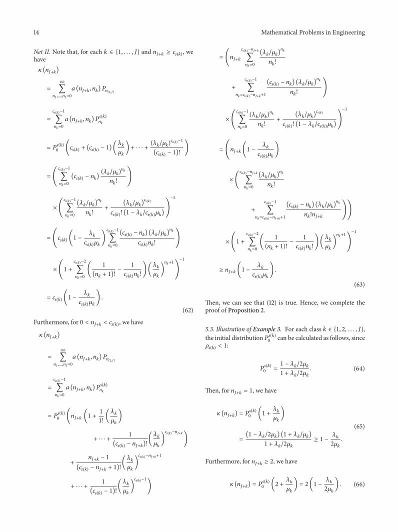
Net II Note that for each 119896 isin 1 119869 and 119899119869+119896 ge 119888119904(119896) wehave120581 (119899119869+119896)
(119888119904(119896) minus 119899119896) (120582119896120583119896)119899119896
119899119896119899119869+119896
))
times (1 +
119888119904(119896)minus2
sum
119899119896=0
(1
(119899119896 + 1)minus
1
119888119904(119896)119899119896) (
120582119896
120583119896
)
119899119896+1
)
minus1
ge 119899119869+119896 (1 minus120582119896
119888119904(119896)120583119896
)
(63)
Then we can see that (12) is true Hence we complete theproof of Proposition 2
53 Illustration of Example 3 For each class 119896 isin 1 2 119869the initial distribution119875119904(119896)0 can be calculated as follows since120588119904(119896) lt 1
2 (1 minus 1205821198962120583119896 minus 120582119869+1198962120583119869+119896) 1205832119869+119896
lt 1
(69)
that is the condition (12) holds
6 Conclusion
The research conducted in the paper is to iteratively derivethe product-form solutions of stationary distributions for a
particular type of preemptive priority multiclass queueingnetworkswithmultiserver stationsThis type of queueing sys-tems can typically be used to model the stochastic dynamicsof some large scale backbone networks with multiprocessorshared-memory switches or local (edge) cloud computingcenters with parallel-server pools The queueing networksare Markovian with exponential interarrival and servicetime distributions The obtained iterative solutions can beused to conduct performance analysis or as comparisoncriteria for approximation and simulation studies Numericalcomparisons with existing Brownian approximating modelrelated to general interarrival and service times are providedto show the effectiveness of our current designed algorithmand our former derived BAM Furthermore based on theiterative solutions we also give some analysis concerningnetwork stability for some cases of these queueing systemswhich provides some insight for more general study
Conflict of Interests
The author declares that there is no conflict of interestsregarding the publication of this paper
Acknowledgments
Partial results graphs and tables are briefly summarized andreported in MICAIrsquo06 This enhanced version with completeproofs of results and latest discussions is a journal versionof the short conference report This research is supported byNational Natural Science Foundation of China with Grantsnos 10371053 10971249 and 11371010
References
[1] S J Mullender and T L Wood ldquoCloud computing new oppor-tunities for telecom providersrdquo Bell Labs Technical Journal vol17 no 2 pp 1ndash4 2012
[2] P Mell and T Grance ldquoThe NIST definition of cloud com-putingrdquo NIST Special Publication 800-145 National Instituteof Standards and Technology US Department of CommerceGaithersburg Md USA 2011
[3] J Rhoton and R Haukioja Cloud Computing ArchitectedSolution DesignHandbook Recursive LimitedWellington NewZealand 2013
[4] F A Tobagi ldquoFast packet switch architectures for broadbandintegrated services digital networksrdquo Proceedings of the IEEEvol 78 no 1 pp 133ndash167 1990
[5] M H L Rao and R Tripathi ldquoFPGA implementation ofreconfigurable switch architecture for next generation commu-nication networksrdquo International Journal of Engineering andTechnology vol 4 no 6 pp 770ndash773 2012
[6] W Dai ldquoOptimal rate scheduling via utility-maximization for119869-user MIMO Markov fading wireless channels with coopera-tionrdquo Operations Research vol 61 no 6 pp 1450ndash1462 2013
[7] M Schwarz Broadband Integrated Networks Prentice HallUpper Saddle River NJ USA 1996
[8] I Nikolaidis and I F Akyildiz ldquoAn overview of source char-acterization in ATM networksrdquo in Modeling and Simulationof Computer and Communications Networks Techniques Tools
16 Mathematical Problems in Engineering
and Tutorials J Walrand K Bachi and G Zobrist Eds pp123ndash150 Gordon and Breach Publishing 1997
[9] W Dai ldquoOn the conflict of truncated random variable vsheavy-tail and long range dependence in computer andnetworksimulationrdquo Journal of Computational Information Systems vol7 no 5 pp 1488ndash1499 2011
[10] W Dai ldquoHeavy traffic limit theorems for a queue with PoissonONOFF long-range dependent sources and general servicetime distributionrdquoActaMathematicae Applicatae Sinica vol 28no 4 pp 807ndash822 2012
[11] J Cao W S Cleveland D Lin and D X Sun ldquoInternet traffictends to poisson and independent as the load increasesrdquo BellLabs Technical Report 2001
[12] W Dai Brownian approximations for queueing networks withfinite buffers modeling heavy traffic analysis and numericalimplementations [PhD thesis] Georgia Institute of TechnologyAtlanta Ga USA 1996
[13] W Dai ldquoDiffusion approximations for multiclass queueingnetworks under preemptive priority service disciplinerdquo AppliedMathematics and Mechanics vol 28 no 10 pp 1331ndash1342 2007
[14] J G Dai andW Dai ldquoA heavy traffic limit theorem for a class ofopen queueing networks with finite buffersrdquoQueueing Systemsvol 32 pp 5ndash40 1999
[15] X Shen H Chen J G Dai and W Dai ldquoThe finite elementmethod for computing the stationary distribution of an SRBMin a hypercube with applications to finite buffer queueingnetworksrdquo Queueing Systems vol 42 no 1 pp 33ndash62 2002
[16] R Serfozo Introduction to Stochastic Networks Springer NewYork NY USA 1999
[17] F Baskett KMChandy R RMuntz and FG Palacios ldquoOpenclosed and mixed networks of queues with different classes ofcustomersrdquo Journal of the Association for ComputingMachineryvol 22 pp 248ndash260 1975
[18] P G Harrison ldquoReversed processes product forms and a non-product formrdquo Linear Algebra and Its Applications vol 386 pp359ndash381 2004
[19] P G Harrison ldquoProcess algebraic non-product-formsrdquo Elec-tronic Notes in Theoretical Computer Science vol 151 no 3 pp61ndash76 2006
[20] W Dai ldquoProduct-form solutions for integrated services packetnetworksrdquo in Proceedings of the 5th Mexican InternationalConference on Artificial Intelligence (MICAI rsquo06) pp 296ndash308IEEE November 2006
[21] H Chen and D Yao Fundamentals of Queueing NetworksSpringer New York NY USA 2001
[22] J G Dai D H Yeh and C Zhou ldquoThe QNET methodfor re-entrant queueing networks with priority disciplinesrdquoOperations Research vol 45 no 4 pp 610ndash623 1997
[23] J M Harrison Brownian Motion and Stochastic Flow SystemsWiley New York NY USA 1985
[24] J R Jackson ldquoNetworks of waiting linesrdquo Operations Researchvol 5 pp 518ndash521 1957
Figure 1 An integrated services cloud computing based network
nonreal time traffic packets (eg data) which can toleratehigher delay but demand much smaller packet loss ratiosHence efficient switching and buffer management schemesare needed for switches
Currently three basic techniques (see eg Tobagi [4]and Rao and Tripathi [5]) are designed to realize the switch-ing function space-division shared-medium and shared-memory In our switches the shared-memory techniqueis employed which is comprised of a single dual-portedmemory shared by all input and output lines Packets arrivingalong input lines are multiplexed into a single stream that isfed to the common memory for storage Inside the memorypackets are organized into different output buffers one foreach output line In each output buffer memory can befurther divided into priority output queues one for eachtype of traffic In the meantime an output stream of packetsis formed by retrieving packets from the output queuessequentially one per queue Among different traffic typespackets are retrieved according to their priorities Inside eachtype packets are retrieved under the first-in first-out (FIFO)service discipline Then the output stream is demultiplexedand packets are transmitted on the output lines There aresome other ways to deal with the output queues such asprocessor sharing among output lines (see eg Tobagi [4]and Rao and Tripathi [5]) We will address these issueselsewhere (see eg Dai [6])
In addition to switching queueing is another main func-tionality of packet switches The introduction of queueingfunction is owing tomultiple packets arriving simultaneouslyfrom separate input lines and owing to the randomness ofpacket arrivals fromboth outside routing and internal routingof the network There are three possibilities for queueing in aswitch input queueing output queueing and shared-memoryqueueing (see eg Schwarz [7] and Rao and Tripathi [5])Shared-memory-queueing mechanism is employed in ourswitches since it has numerous advantages with respect toswitching and queueing over other schemes For exampleboth switching and queueing functions can be implementedtogether by controlling the memory read and write properlyFurthermore modifying the memory read and write control
Switch 1
Exit
External arrivals
Class 3
Exit
Feedback
Class 1
Switch 2
2
1
21
ExitClass 4
Feedback
Class 2
c1
c2
Figure 2 A two-type and four-class network with twomultiproces-sor switches Type 1 includes class 1 and class 2 Type 2 consists ofclass 3 and class 4 Type 1 owns the service priority
2 times 2
2 times 2
2 times 2
2 times 2
Figure 3 A two-stage switchwith four dual-ported shared-memoryswitching modules
circuit makes the shared-memory switch sufficiently flexibleto perform functions such as priority control and otheroperations
Nevertheless no matter what technology is employedin implementing the switch it places certain limitationson the size of the switch and line speeds Currently twopossible ways can be used to build large switches tomatch thetransmission speed of optical fiber The first one is to adoptparallel processors (see eg Figure 2) The second one is tointerconnect many switches (known as switch modules) ina multistage configuration to build large switches (see egFigure 3) The remaining issue is how to reasonably allocateresources of these switches and efficiently evaluate the systemperformance
The statistical characteristics of packet interarrival timesand packet sizes have a major impact on switch hardwareand software designs owing to the consideration of networkperformance How to more effectively identify packet trafficpatterns is a very active and involved research field (see egNikolaidis and Akyildiz [8] and Dai [6 9 10]) Independentand identical distribution (iid) is the popular assumptionfor these times and packet sizes Doubly stochastic renewalprocess introduced in Dai [6] is the latest definition andgeneralization related to input traffic and service processesfor a wireless network under random environment Theeffectiveness of these characteristics is supported by recentdiscoveries in Cao et al [11] and Dai [9 10]
Mathematical Problems in Engineering 3
In all circumstances it is imperative to find product-form solutions for those queueing networks under suit-able conditions to conduct performance analysis or providecomparison criteria to show the effectiveness of approxi-mation andor simulation studies (see eg Dai et al [612ndash15]) Furthermore note that the stochastic dynamics ofthe backbone networks with multiprocessor shared-memoryswitches and the local (edge) cloud computing centers withparallel-server pools in Figure 1 can both be described by amulticlass queueing networks with parallel servers at eachstation Hence in this paper we aim to derive the product-form solutions iteratively for one particular type of relatedqueueing networks that is a type of particular preemptivepriority multiclass queueing networks when the interarrivaland service times are exponentially distributed In additionwe also aim to provide some numerical comparisons withexisting Brownian approximating model (BAM) related togeneral interarrival and service times to show the effec-tiveness of our current designed algorithm and our formerderived BAM
Next we provide some review of the existing literatureassociated with the current study Comparisons between theexisting studies and our current discussion are also presented
Under a general Whittle network framework theproduct-form solutions are presented in Serfozo [16] forsome multiclass networks which include those with sector-dependent (eg Example 33) and class-station-dependentservice rates (eg BCMP networks in Section 33 whichare introduced by Baskett et al [17]) Without consideringthe interaction among different stations the distinguishingfeature of these networks is that a jobrsquos service rate at astation may consist of two intensities one referred to asstation intensity is a function of the total queue length atthe station and the other one referred to as class intensity isa function of the queue length in the same class as the jobbeing served Some specific single-class queueing systems ofBCMP networks in Section 33 of Serfozo [16] are revisited inHarrison [18 19] by developing some Reversed CompoundAgent Theorem (RCAT) based method The correspondingproduct-form and non-product-form solutions are derivedNevertheless as claimed inHarrison [18 19] heavier notationwill be involved as long as a multiclass BCMP network isconcerned
Although our networks are of a form of those networkswithmultiple types of units as introduced in Serfozo [16] ournetworks are beyond those with sector-dependent and class-station-dependent service rates as introduced previouslyMore precisely for a station in our networks the stationintensity is not only a function of the total queue length butalso a function of combinations of queue lengths of variousclasses The class intensity depends on not only the queuelength of itself andor the total queue length but also thenumbers of jobs in other classes at the station Thereforehow to find suitable functionΦ and how to prove our servicerates to be Φ-balanced as defined in Chapter 3 of Serfozo[16] are not obvious Moreover how to apply the RCATbasedmethod developed inHarrison [18 19] to ourmulticlassnetwork cases is also not trivial Thus in this paper we usethe method of solving Kolmogorov (balance) equations to
get the product-form solutions iteratively which are moreengineering and computationally friendly Furthermore bythis method we can also give some analysis concerningnetwork stability for some cases of these systems whichprovides some insight for more general study
The remainder of this paper is organized as follows Theopen priority multiclass queueing network associated withhigh-speed ISPN is described in Section 2 Our main resultsincluding product-form solutions and performance compar-isons are presented in Section 3 Numerical comparisonsare given in Section 4 The proofs of our main theoremsare provided in Section 5 The conclusion of the paper ispresented in Section 6
2 The Queueing Network Model
Note that the stochastic dynamics of the backbone corenetworks with multiprocessor shared-memory switches andthe local (edge) cloud computing centers with parallel-serverpools in Figure 1 can both be described by multiclass queue-ing networks with parallel servers at each station Thereforewe consider a queueing network that has 119869 multiserverstations Each station indexed by 119895 isin 1 119869 owns 119888119895 serversand has an infinite capacity waiting buffer In the networkthere are 119868 job types Each type consists of 119869 job classes thatare distributed at different stations Therefore the networkis populated by 119870 (= 119868119869) job classes which are labeled by119896 isin 1 119870 Upon the arrival of a job of a type fromoutside the network it may only receive service for part of119869 classes and may visit a particular class more than once (butat most finite many times) Then it leaves the network (iethe network is open) At any given time during its lifetime inthe network the job belongs to one of the classes and changesclasses at each time a service is completed All jobs within aclass are served at a unique station and more than one classmight be served at a station (so-called multiclass queueingnetwork) The ordered sequence of classes that a job visits inthe network is named a route Interrouting among differentjob types is not allowed throughout the entire network
We use C(119895) to denote the set of classes belonging tostation 119895 Let 119904(119896) denote the station to which class 119896 belongsWe implicitly set 119895 = 119904(119896) when 119895 and 119896 appear togetherAssociated with each class 119896 there are two iid sequencesof random variables (rv) 119906119896 = 119906119896(119894) 119894 ge 1 and V119896 =V119896(119894) 119894 ge 1 an iid sequence of 119870-dimensional randomvectors 120601119896 = 120601119896(119894) 119894 ge 1 and two real numbers 120572119896 ge 0and119898119896 = 1120583119896 gt 0 We suppose that the 3119870 sequences
1199061 119906119870 V1 V119870 1206011 120601
119870 (1)
are mutually independent The initial rvs 119906119896(1) and V119896(1)have means 119864[119906119896(1)] = 1120572119896 and 119864[V119896(1)] = 119898119896 respectivelyFor each 119894 isin 1 2 119906119896(119894) denotes the interarrival timebetween the (119894 minus 1)th and the 119894th externally arrival job at class119896 Furthermore V119896(119894) denotes the service time for the 119894th class119896 job In addition 120601119896(119894) denotes the routing vector of the 119894thclass 119896 job We allow 120572119896 = 0 for some classes 119896 isin E equiv 119896
120572119896 = 0Then it follows that 120572119896 and 120583119896 are the external arrivalrate and service rate for class 119896 respectively We assume that
4 Mathematical Problems in Engineering
the routing vector 120601119896(119894) takes values in 1198900 1198901 119890119870 where1198900 is the 119870-dimensional vector of all 0rsquos For 119897 = 1 119870 119890119897is the 119870-dimensional vector with 119897th component 1 and othercomponents 0 When 120601119896(119894) = 119890119897 the 119894th job departing class 119896becomes a class 119897 job Let119901119896119897 = 119875120601
119896(119894) = 119890119897 be the probability
that a job departing class 119896 becomes a class 119897 job (of the sametype) Thus the corresponding 119870 times 119870 matrix 119875 = (119901119896119897) isrouting matrix of the network Furthermore the matrix
is finite that is (119868 minus 1198751015840) is invertible with Q = (119868 minus 1198751015840)minus1 sincethe network is open The symbol 1015840 on a vector or a matrixdenotes the transpose and 119868 denotes the identity matrix
We use 120582119896 for 119896 isin 1 119870 to denote the overall arrivalrate of class 119896 including both external arrivals and internaltransitions Then we have the following traffic equation
120582119896 = 120572119896 +
119870
sum
119897=1
120582119897119901119897119896 (3)
or in its vector form 120582 = 120572+1198751015840120582 (all vectors in this paper areto be interpreted as column vectors unless explicitly statedotherwise) Note that the unique solution 120582 of (3) is given by120582 = Q120572 For each 120582119896 if there is a long-run average rate offlow into the class which equals the long-run average rate outof that class this rate will equal 120582119896 Furthermore we definethe traffic intensity 120588119895 for station 119895 as follows
120588119895 = sum
119896isinC(119895)
120582119896
119888119895120583119896
(4)
where 120588119895 with 120588119895 le 1 is also referred to as the nominal fractionof time that station 119895 is nonidle
The order of jobs being served at each station is dictatedby a service discipline In the current research we restrictour attention to static buffer priority (SBP) service disciplinesunder which the classes at each station are assigned a fixedrank (with no ties) In our queueing network each type ofjobs is assigned the same priority rank at every station whereit possibly receives service When a server within a stationswitches from one job to another the new job will be takenfrom the leading (or longest waiting) job at the highest ranknonempty class at the serverrsquos station Within each class it isassumed that jobs are served on the first-in first-out (FIFO)basis We suppose that the discipline employed is nonidlingthat is a server is never idle when there are jobs waiting tobe served at its station We also assume that the disciplineis preemptive resume that is when a job arrives at a stationwith all servers busy and if the job is with a higher rank thanat least one of the jobs currently being served one of thelower rank job services is interrupted when there is a serveravailable to the interrupted service it continues fromwhere itleft off For convenience and without loss of generality we useconsecutive numbers to index the classes that have the samepriority rank at stations 1 to 119869 In other words the highestpriority classes for station 1 to 119869 are indexed by 1 to 119869 thesecond highest priority classes are indexed by 119869 + 1 to 2119869
and the lowest priority classes are indexed by119870minus119869+1 to119870 Anexample of such a two-station network is given in Figure 2 Inthe network type 1 traffic possibly requires class 1 and class2 services type 2 traffic possibly requires class 3 and class 4services and classes in type 1 have the higher priority at theircorresponding stations
Finally we define the cumulative arrival cumulativeservice and cumulative routing processes by the followingsums
119880119896 (119899) =
119899
sum
119894=1
119906119896 (119894) 119881119896 (119899) =
119899
sum
119894=1
V119896 (119894)
Φ119896(119899) =
119899
sum
119894=1
120601119896(119894)
(5)
where the 119897th component Φ119896119897 (119899) of Φ119896(119899) is the cumulative
number of jobs to class 119897 for the first 119899th jobs leaving class 119896with 119899 = 1 2 and 119896 119897 isin 1 119870 Then we define
119864119896 (119905) equiv max 119899 ge 0 119880119896 (119899) le 119905
119878119896 (119905) equiv max 119899 ge 0 119881119896 (119899) le 119905
Note that 119864119896(119905) denotes the total number of external arrivalsto class 119896 in time interval [0 119905] 119878119896(119905) represents the totalnumber of class 119896 jobs which have finished service in [0 119905]119860119896(119905) is the total arrivals to class 119896 in [0 119905] including bothexternal arrivals and internal transitions
3 Steady-State Queue Length Distributions
We use 119876119896(119905) to denote the number of class 119896 jobs in station119895 = 119904(119896) with 119895 isin 1 2 119869 and 119896 isin 1 2 119870 at time119905 It is called the queue length process for class 119896 jobs Forconvenience let119876(119894119895)(119905) and 119899(119894119895) be the (119895minus119894+1)-dimensionalqueue length process and (119895minus119894+1)-dimensional state vectorsrespectively They are given by
for 119895 gt 119894 and 119894 119895 isin 1 2 119870 and nonnegative integers119899119894 119899119895 Then we use 119875119899(1119870)(119905) to denote the probability ofsystem at state 119899(1119870) = (1198991 119899119870) and at time 119905 that is
denote the corresponding steady-state probability of systemat state (1198991 119899119870) if the network exists in a stationarydistribution In addition let 119875119904(119894119869+119896)119899119894119869+119896
denote the probabilityat state 119899119894119869+119896 for class 119894119869 + 119896 with 119894 isin 0 1 119868 minus 1 and119896 isin 1 2 119869
Mathematical Problems in Engineering 5
Under the usual convention let 119909 and 119910 denote the smallerone of any two real numbers 119909 and 119910 Let 119909 or 119910 denote thelarger one of 119909 and 119910 that is 119909 and 119910 equiv min119909 119910 and 119909 or119910 equiv max119909 119910 Then for each 119896 isin 1 119870 we have thefollowing notation
119886 (119909 119910) equiv (119909 and (119888119904(119896) minus 119910)) or 0 (10)
Furthermore for 119894 = 0 define 120581(119899119896) equiv 119899119896 and 119888119904(119896)
Theorem 1 (steady-state distribution) Assume that all of theservice times and external interarrival times are exponentiallydistributed with rates as before and the traffic intensity 120588119895 lt 1for all 119895 isin 1 119869 Furthermore suppose that
for 119899119894119869+119896 gt 0 119894 isin 0 119868 minus 1 and 119896 isin 1 119869 Then foreach ℎ isin 1 2 119868 the steady-state distribution is given bythe following product form
The following theorem relates condition (12) to primitiveinterarrival time and service rates for some cases of thesesystems which provides some insight for more general study
Proposition 2 (network stability condition) Under the expo-nential assumptions as stated in Theorem 1 if 120588119895 lt 1 for each119895 isin 1 119869 the stability condition (12) holds for the followingnetworks
Net I Multiclass networks with single-server stations that isthe number 119888119895 of servers is one for all stations 119895 isin 1 119869while the number 119868 of job types can be arbitrary
Net II The number 119888119895 of servers can be arbitrary for all stations119895 isin 1 119869 while the number of job types equals two (119868 = 2)
Table 1 Numerical tests for network stability condition (12)
We conjecture that 120588119895 lt 1 for 119895 isin 1 119869 impliesthe condition (12) for our general network Neverthelessowing to complex computation involved the correspondinganalytical illustration is not a trivial task
Example 3 Consider a network with three job types (119868 = 3)and at least one station 119895 = 119904(119896) having two servers (119888119904(119896) = 2for 119896 isin 1 119869) while other stations have at most twoservers (119888119904(119897) le 2 for 119897 isin 1 2 119869 119896) For a station119904(119896) with three servers the condition (12) can be explicitlyexpressed as follows
(1205822119869+119896
1205832119869+119896
times(1 +120582119896
120583119896
+120582119869+119896
2120583119869+119896
minus (120582119896
2120583119896
)
2
minus1
4(120582119896
120583119896
)
3
+120582119896120582119869+119896
4120583119896120583119869+119896
))
times (2(1 minus120582119896
2120583119896
minus120582119869+119896
2120583119869+119896
)
times (1 +120582119896
120583119896
+120582119869+119896
2120583119869+119896
minus (120582119896
2120583119896
)
2
minus1
4(120582119896
120583119896
)
3
+ 2(1 minus120582119896
2120583119896
)120582119896120582119869+119896
4120583119896120583119869+119896
))
minus1
lt 1
(16)
for 1198992119869+119896 ge 2 Under 120588119895 lt 1 it is easy to see that the aboveinequality is true if 120582119896120583119896 le 1 Numerical tests in Table 1have also been conducted and show that the inequality is trueeven for 1 lt 120582119896120583119896 lt 2 but the corresponding analyticdemonstration could be nontrivial The detailed illustrationof the example will be provided at the end of this paper
Remark 4 The justifications of Theorem 1 and Proposition 2are postponed to Section 5 Instead we will first use theseresults as comparison criteria to illustrate the effectivenessof the diffusion approximation models developed in Dai[13] and answer the question on when these approximationmodels can be employed
4 Numerical Comparisons
First of all we note that partial results presented in thissection were briefly reported in the short conference version(Dai [20]) of this paper More precisely we consider anetwork with single-server station and under preemptive
6 Mathematical Problems in Engineering
priority service discipline By employing the exact solutionsdeveloped in previous sections we conduct performancecomparisons between these product-form solutions and theapproximating ones of Brownian network models
Brownian network models which are also known assemimartingale reflecting Brownian motions (SRBM) havebeen widely employed as approximating models for multi-class queueing networks with general interarrival and servicetime distributions when the traffic intensity defined in (4)is suitably large or close to one (see eg Dai [13]) Theeffectiveness of the Brownian network models has beenjustified in numerical cases by comparing their solutions witheither exact solutions or simulation results (see eg Dai [13]Chen and Yao [21] and Dai et al [22]) Thus it is meaningfulto illustrate the correctness of our newly derived formula bycomparing it with the Brownian network models
For the network with exponential interarrival and servicetime distributions by using Theorem 1 we get the steady-state mean queue length for each class 119896 isin 1 119870 as
119864119876119896 (infin) =
infin
sum
119899119896=0
119899119896119875119904(119896)119899119896
=120582119896119898119896
1 minus sum119896119894=1 120582119894119898119894
=120572119896119898119896 (1 minus 119901119896119896)
1 minus sum119896119894=1 120572119894119898119894 (1 minus 119901119894119894)
(17)
and the expected total time (sojourn time) a job had to spendin the system as
119864119879119896 (infin) =119898119896
1 minus sum119896119894=1 120582119894119898119894
=119898119896
1 minus sum119896119894=1 120572119894119898119894 (1 minus 119901119894119894)
(18)
For the networkwith general interarrival and service timedistributions owing to the nature of our network routingstructure the higher priority classes are independent of lowerones Then it follows from the studies in Dai [13] Harrison[23] and Chen and Yao [21] that the steady-state meansojourn time and mean queue length for each class 119896 caniteratively be calculated with respect to priority order asfollows
where 119864119882119896(infin) is the steady-state mean total workload forall classes 119894 isin 1 119896 and 119896 = 1 119870 More precisely it isgiven by
1198982119894 (1205723119894 119886119894 + 120582119894119901119894119894 (1 minus 119901119894119894))
(1 minus 119901119894119894)2
)
(21)
and 119886119894 119887119894 are the variances of interarrival and service timesequences for each class 119894
In our numerical comparisons we consider an exponen-tial networkwith119870 = 3 For this case our corresponding dataare listed in Table 2 In the table ERROR = SRBM minus EXACTand RATIO = (|ERROR|EXACT) lowast 100 119864119876(infin) =
sum3119894=1 119864119876119894(infin) and 119864119896(infin) = sum
119896119894=1 119879119894(infin) for 119896 = 1 2 3
From the table we can see that SRBMs are more reasonableapproximations of their physical queueing counterpartswhentraffic intensities for the lowest priority jobs are relativelylarge
5 Proofs of Theorem 1 and Proposition 2
51 Proof of Theorem 1 For convenience we introduce someadditional notations Let Δ119864119896(119905) Δ119878119896(119905) and Δ119860119896(119905) bedefined by
Δ119864119896 (119905) equiv 119864119896 (119905 + Δ119905) minus 119864119896 (119905)
Δ119878119896 (119905) equiv 119878119896 (119905 + Δ119905) minus 119878119896 (119905)
Δ119860119896 (119905) equiv 119860119896 (119905 + Δ119905) minus 119860119896 (119905)
(22)
which denote the cumulative external arrivals to class 119896 thecumulative number of jobs finished services at class 119896 andthe total arrivals to class 119896 in [119905 119905 + Δ119905] Then we can justifyTheorem 1 by induction as in the following several steps
Step 1 We consider the steady-state distribution for thehighest rank classes with each index 119896 isin 1 2 119869 Inthis case the type index 119894 = 0 is used in Theorem 1 Owingto the preemptive-resume service discipline and the classrouting structure we know that these 119869 classes form a Jacksonnetwork Then by the theorem in Jackson [24] we have thefollowing product form
where 119875119904(119896)119899119896 denotes the steady-state probability at state 119899119896 forclass 119896 (isin 1 2 119869) at station 119904(119896) More precisely it isgiven by
where the second equality follows from the preemptiveassumption and 119875119899(1119869)119899(119869+12119869)(119905) is the conditional probabilityat time 119905 for classes with 119896 isin 1 119869 at state 119899(1119869) in termsof classes with 119896 isin 119869 + 1 2119869 at state 119899(119869+12119869) that is
In order to get the steady state distribution for 119875119899(119869+12119869)(119905) weconsider each state 119899(119869+12119869) at time 119905 for the second highest
rank class jobsThere are several ways inwhich the system canreach it They can be summarized in the following formula
119875119899(119869+12119869)(119905 + Δ119905)
= (1 minus
119869
sum
119896=1
120572119869+119896Δ119905
minus
119869
sum
119896=1
infin
sum
1198991119899119869=0
119886 (119899119869+119896 119899119896) 120583119869+119896 (1 minus 119901119869+119896119869+119896)
times 119875119899119869+1 119899119869+119896+11198992119869(119905)
+
119869
sum
119896=1
(119899119869+119896 and 1) 120572119869+119896Δ119905119875119899119869+1 119899119869+119896minus11198992119869(119905)
+
119869
sum
119903119904=1119904 =119903
(
infin
sum
1198991 119899119869=0
119886 (119899119869+119903 + 1 119899119903)
times 120583119869+119903119901119869+119903119869+119904119875119899(1119869)(119905))
times (119899119869+119904 and 1) Δ119905119875119899119869+1 119899119869+119903+1119899119869+119904minus11198992119869(119905)
+ 119900 (Δ119905)
(28)
where 119886(119899119869+119896 119899119896) = (119899119869+119896 and (119888119904(119896) minus 119899119896)) or 0 as defined in (10)119900(Δ119905) is infinitesimal in terms of Δ119905 that is 119900(Δ119905)Δ119905 rarr 0 asΔ119905 rarr infin Equation (28) can be illustrated in the followingdisjoint events
EventA The 119869-dimensional queue length process119876(119869+12119869)(119905)keeps at state 119899(119869+12119869) unchanging at times 119905 and 119905 + Δ119905 thatis
Part One Suppose Δ119878119869+119896(119905) = Δ119860119869+119896(119905) = 0 for all 119896 isin
1 2 119869 that is no external jobs arrive to classes withindices belonging to 119869 + 1 2119869 during [119905 119905 + Δ119905] while nojobs finish their services either because the jobs being servedat time 119905 require longer service times than Δ119905 or because theservices are blocked or interrupted by higher rank class jobsThen the probability for Part One can be expressed in thefollowing product form
To explain the fourth equality of (30) we introduce morenotations Let 119887119896(119905)Δ119905 denote the probability that Δ119860119896(119905) = 1for 119896 isin 1 119869 and let 119888119869+119896(119905)Δ119905 be the probability thatsum119896minus1119904=1 Δ119878119869+119904(119905) = 1 for 119896 isin 2 3 119869 that is
These probabilities can be explicitly expressed in terms of theexternal arrival rates service rates and network states forexample
119887119896 (119905) Δ119905 = (120572119896 + sum
119897isin1119869
119901119897119896120583119897 (119888119904(119897) and 119876119897 (119905)))Δ119905 (34)
Thus by the independent assumptions on external arrival andservice processes among different stations and classes and foreach 119896 isin 2 3 119869 we have
= (1 minus 119886119869+119896 (119905) 120583119869+119896Δ119905) (1 minus 120572119869+119896Δ119905)
times (1 minus 119887119896 (119905) Δ119905) (1 minus 119888119869+119896 (119905) Δ119905)
+ (1 minus ((119876119869+119896 (119905) and (119888119904(119896) minus (119876119896 (119905) + 1))) or 0) 120583119869+119896Δ119905)
times (1 minus 120572119869+119896Δ119905)
times (119887119896 (119905) Δ119905 minus 119901119896119896120583119896 (119888119904(119896) and 119876119896 (119905)) Δ119905)
times (1 minus 119888119869+119896 (119905) Δ119905)
+ (1 minus ((119876119869+119896 (119905) and (119888119904(119896) minus 119876119896 (119905))) or 0) 120583119869+119896Δ119905)
times (1 minus 120572119869+119896Δ119905)
times 119901119896119896120583119896 (119888119904(119896) and 119876119896 (119905)) Δ119905 (1 minus 119888119869+119896 (119905) Δ119905)
+ (1 minus (((119876119869+119896 (119905) + 1) and (119888119904(119896) minus 119876119896 (119905))) or 0) 120583119869+119896Δ119905)
times (1 minus 120572119869+119896Δ119905) (1 minus 119887119896 (119905) Δ119905) 119888119869+119896 (119905) Δ119905
+ 119900 (Δ119905)
= 1 minus 120572119869+119896Δ119905 minus 119886119869+119896 (119905) 120583119869+119896Δ119905 + 119900 (Δ119905)
(35)
For the case 119896 = 1 one can use the similar way to check thatthe result in the above equation is also true
Part Two Suppose Δ119878119869+119896(119905) = Δ119860119869+119896(119905) ge 1 for at least one119896 isin 1 2 119895 that is the number (at least one) of jobs
that finished their services for class 119869 + 119896 in [119905 119905 + Δ119905] equalsthat of jobs that arrived at the class It is easy to see that theprobability corresponding part one is given by
119875 Δ119878119869+119896 (119905) = Δ119860119869+119896 (119905) ge 1
times 119875 119876(1119869) (119905) = 119899(1119869)
times 119875 119876(119869+12119869) (119905) = 119899(119869+12119869) + 119900 (Δ119905)
= (1 minus
119869
sum
119896=1
120572119869+119896Δ119905
minus
119869
sum
119896=1
infin
sum
1198991 119899119869=0
119886 (119899119869+119896 119899119896) 120583119869+119896 (1 minus 119901119869+119896119869+119896) 119875119899(1119869)(119905) Δ119905)
times 119875119899(119869+12119869)(119905) + 119900 (Δ119905)
(37)
EventBThere is a 119896 isin 1 119869 such that119876119869+119896(119905) = 119899119869+1+1119876119869+119896(119905 + Δ119905) = 119899119869+1 and for all 119897 isin 1 119869 119896 119876119869+119897(119905) =119876119869+119897(119905 + Δ119905) = 119899119869+119897 Similar to the discussion in EventA wecan obtain the probability for EventB as follows
times 119875119899119869+1119899119869+119896+11198992119869(119905) + 119900 (Δ119905)
(38)
EventC There is a 119896 isin 1 119869 such that119876119869+119896(119905) = 119899119869+119896 minus1119876119869+119896(119905 + Δ119905) = 119899119869+119896 and for all 119897 isin 1 119869 119896 119876119869+119897(119905) =119876119869+119897(119905 +Δ119905) = 119899119869+119897 Then we can get the probability for EventC as follows119869
(119899119869+119896 and 1) 120572119869+119896Δ119905119875119899119869+1 119899119869+119896minus11198992119869(119905) + 119900 (Δ119905)
(39)
EventDThere exist 119903 119904 isin 1 119869 such that119876119869+119903(119905) = 119899119869+119903+1119876119869+119903(119905+Δ119905) = 119899119869+119904119876119869+119904(119905) = 119899119869+119904minus1 and119876119869+119904(119905+Δ119905) = 119899119869+119904and for all 119897 isin 1 119869 119903 119904 119876119869+119897(119905) = 119876119869+119897(119905 + Δ119905) = 119899119869+119897Then we can get the probability for EventD as follows
times (119899119869+119904 and 1) 119875119899119869+1119899119869+119903+1119899119869+119904minus11198992119869(119905)
(41)
Mathematical Problems in Engineering 11
Next we show that the given distribution correspondingℎ = 2 in Theorem 1 is a steady-state solution of thoseequations described by (41) It is enough to demonstrate thatthe derivatives in the above equations are all made zero bysetting 119875119899(12119869)(119905) = 119875119899(12119869) that is to prove that
Then substituting (47) into (46) we get the necessaryequality
Next we derive the initial distribution119875119904(119869+119896)0 correspond-ing to state 119899119869+119896 = 0 By the network stability conditions(12) and 120588119895 lt 1 for each 119895 isin 1 119869 it follows fromsuminfin119899119869+119896=0
119875119904(119869+119896)119899119869+119896
= 1 that the following initial distribution iswellposed
Hence we complete the proof ofTheorem 1 for priority typesℎ isin 1 2
Step 3 To finish the induction procedure in this step we firstsuppose that the result described in Theorem 1 is true for allclasses with priority rank ℎ isin 1 119868minus1 then we show thatit is true for all classes with priority rank ℎ isin 1 119868 By
12 Mathematical Problems in Engineering
the similar illustration in getting (41) we have the followingdifferential equations
times 119875119899(119868minus1)119869+1119899(119868minus1)119869+119896+1119899119868119869(119905)
+
119869
sum
119896=1
(119899(119868minus1)119869+119896 and 1) 120572(119868minus1)119869+119896
times 119875119899(119868minus1)119869+1119899(119868minus1)119869+119896minus1119899119868119869(119905)
+
119869
sum
119903119904=1119904 =119903
infin
sum
1198991 119899(119868minus1)119869=0
119886(119899(119868minus1)119869+119903 + 1
119868minus2
sum
119906=0
119899119906119869+119903)
times 120583(119868minus1)119869+119903119901(119868minus1)119869+119903(119868minus1)119869+119904
times 119875119899(1(119868minus1)119869)(119905) (119899(119868minus1)119869+119904 and 1)
times 119875119899(119868minus1)119869+1119899(119868minus1)119869+119903+1119899(119868minus1)119869+119904minus1119899119868119869(119905)
(49)
Next we show that the given distribution corresponding thelowest priority type inTheorem 1 is a steady-state solution ofthose equations described by (49) It suffices to demonstratethat the derivatives in the above equations are all made zeroby setting 119875119899((119868minus1)119869119868119869)(119905) = 119875119899((119868minus1)119869119868119869) that is to prove that
times 119875119899(119868minus1)119869+1119899(119868minus1)119869+119896+1119899119868119869
+
119869
sum
119896=1
(119899(119868minus1)119869+119896 and 1) 120572(119868minus1)119869+119896119875119899(119868minus1)119869+1119899(119868minus1)119869+119896minus1119899119868119869
+
119869
sum
119903119904=1119904 =119903
infin
sum
1198991119899(119868minus1)119869=0
119886(119899(119868minus1)119869+119903 + 1
119868minus2
sum
119906=0
119899119906119869+119903)
times 119875119899(1(119868minus1)119869)120583(119868minus1)119869+119903
times 119901(119868minus1)119869+119903(119868minus1)119869+119904 (119899(119868minus1)119869+119904 and 1)
times 119875119899(119868minus1)119869+1119899(119868minus1)119869+119903+1119899(119868minus1)119869+119904minus1119899119868119869
times 119875119899(119868minus1)119869+1119899(119868minus1)119869+119896+1119899119868119869
+
119869
sum
119896=1
(119899(119868minus1)119869+119896 and 1) 120572(119868minus1)119869+119896119875119899(119868minus1)119869+1119899(119868minus1)119869+119896minus1119899119868119869
+
119869
sum
119903119904=1119904 =119903
120581 (119899(119868minus1)119869+119896 + 1)
times 120583(119868minus1)119869+119903119901(119868minus1)119869+119903(119868minus1)119869+119904 (119899(119868minus1)119869+119904 and 1)
times 119875119899(119868minus1)119869+1119899(119868minus1)119869+119903+1119899(119868minus1)119869+119904minus1119899119868119869
Then substituting (55) into (54) we get the necessaryequality
Next we derive the initial distribution 119875119904((119868minus1)119869+119896)0 cor-responding to state 119899(119868minus1)119869+119896 = 0 By the network stabilityconditions (12) and 120588119895 lt 1 for each 119895 isin 1 119869 it follows
Net I We justify the stability condition (12) for Net I byinduction in terms of the number of job types that is ℎ =1 2 119868
First we consider the case that ℎ = 2 Note that 119888119895 = 1 forall 119895 isin 1 2 119869 and step one in the proof ofTheorem 1 wehave that for 119899119869+119896 gt 0 with 119896 isin 1 2 119869
120581 (119899119869+119896) = 119875119904(119896)0 = 1 minus
120582119896
120583119896
(57)
Therefore condition (12) is true for ℎ = 2 Furthermore wehave
119875119904(119869+119896)0 = 1 minus
120582119869+119896
(1 minus 120582119896120583119896) 120583119869+119896
(58)
Second for ℎ le 119868 minus 1 we suppose that
120581 (119899(ℎminus1)119869+119896) = 1 minus
ℎminus2
sum
119894=0
120582119894119869+119896
120583119894119869+119896
(59)
Hence we have
119875119904((ℎminus1)119869+119896)0 = 1 minus
120582(ℎminus1)119869+119896
(1 minus sumℎminus2119894=0 120582119894119869+119896120583119894119869+119896) 120583(ℎminus1)119869+119896
(60)
From the induction assumptions (59) and (60) we know that(12) is true for ℎ le 119868 minus 1
Finally we show that (12) holds for ℎ = 119868 In fact fromthe definition of 120581(119899(119868minus1)119869+119896) we know that for 119899(119868minus1)119869+119896 gt 0
120581 (119899(119868minus1)119869+119896) =
119868minus2
prod
119894=0
119875119904(119894119869+119896)0 = 1 minus
119868minus2
sum
119894=0
120582119894119869+119896
120583119894119869+119896
(61)
Then we see that (12) is true for ℎ = 119868 Hence we completethe proof of Net I
14 Mathematical Problems in Engineering
Net II Note that for each 119896 isin 1 119869 and 119899119869+119896 ge 119888119904(119896) wehave120581 (119899119869+119896)
(119888119904(119896) minus 119899119896) (120582119896120583119896)119899119896
119899119896119899119869+119896
))
times (1 +
119888119904(119896)minus2
sum
119899119896=0
(1
(119899119896 + 1)minus
1
119888119904(119896)119899119896) (
120582119896
120583119896
)
119899119896+1
)
minus1
ge 119899119869+119896 (1 minus120582119896
119888119904(119896)120583119896
)
(63)
Then we can see that (12) is true Hence we complete theproof of Proposition 2
53 Illustration of Example 3 For each class 119896 isin 1 2 119869the initial distribution119875119904(119896)0 can be calculated as follows since120588119904(119896) lt 1
2 (1 minus 1205821198962120583119896 minus 120582119869+1198962120583119869+119896) 1205832119869+119896
lt 1
(69)
that is the condition (12) holds
6 Conclusion
The research conducted in the paper is to iteratively derivethe product-form solutions of stationary distributions for a
particular type of preemptive priority multiclass queueingnetworkswithmultiserver stationsThis type of queueing sys-tems can typically be used to model the stochastic dynamicsof some large scale backbone networks with multiprocessorshared-memory switches or local (edge) cloud computingcenters with parallel-server pools The queueing networksare Markovian with exponential interarrival and servicetime distributions The obtained iterative solutions can beused to conduct performance analysis or as comparisoncriteria for approximation and simulation studies Numericalcomparisons with existing Brownian approximating modelrelated to general interarrival and service times are providedto show the effectiveness of our current designed algorithmand our former derived BAM Furthermore based on theiterative solutions we also give some analysis concerningnetwork stability for some cases of these queueing systemswhich provides some insight for more general study
Conflict of Interests
The author declares that there is no conflict of interestsregarding the publication of this paper
Acknowledgments
Partial results graphs and tables are briefly summarized andreported in MICAIrsquo06 This enhanced version with completeproofs of results and latest discussions is a journal versionof the short conference report This research is supported byNational Natural Science Foundation of China with Grantsnos 10371053 10971249 and 11371010
References
[1] S J Mullender and T L Wood ldquoCloud computing new oppor-tunities for telecom providersrdquo Bell Labs Technical Journal vol17 no 2 pp 1ndash4 2012
[2] P Mell and T Grance ldquoThe NIST definition of cloud com-putingrdquo NIST Special Publication 800-145 National Instituteof Standards and Technology US Department of CommerceGaithersburg Md USA 2011
[3] J Rhoton and R Haukioja Cloud Computing ArchitectedSolution DesignHandbook Recursive LimitedWellington NewZealand 2013
[4] F A Tobagi ldquoFast packet switch architectures for broadbandintegrated services digital networksrdquo Proceedings of the IEEEvol 78 no 1 pp 133ndash167 1990
[5] M H L Rao and R Tripathi ldquoFPGA implementation ofreconfigurable switch architecture for next generation commu-nication networksrdquo International Journal of Engineering andTechnology vol 4 no 6 pp 770ndash773 2012
[6] W Dai ldquoOptimal rate scheduling via utility-maximization for119869-user MIMO Markov fading wireless channels with coopera-tionrdquo Operations Research vol 61 no 6 pp 1450ndash1462 2013
[7] M Schwarz Broadband Integrated Networks Prentice HallUpper Saddle River NJ USA 1996
[8] I Nikolaidis and I F Akyildiz ldquoAn overview of source char-acterization in ATM networksrdquo in Modeling and Simulationof Computer and Communications Networks Techniques Tools
16 Mathematical Problems in Engineering
and Tutorials J Walrand K Bachi and G Zobrist Eds pp123ndash150 Gordon and Breach Publishing 1997
[9] W Dai ldquoOn the conflict of truncated random variable vsheavy-tail and long range dependence in computer andnetworksimulationrdquo Journal of Computational Information Systems vol7 no 5 pp 1488ndash1499 2011
[10] W Dai ldquoHeavy traffic limit theorems for a queue with PoissonONOFF long-range dependent sources and general servicetime distributionrdquoActaMathematicae Applicatae Sinica vol 28no 4 pp 807ndash822 2012
[11] J Cao W S Cleveland D Lin and D X Sun ldquoInternet traffictends to poisson and independent as the load increasesrdquo BellLabs Technical Report 2001
[12] W Dai Brownian approximations for queueing networks withfinite buffers modeling heavy traffic analysis and numericalimplementations [PhD thesis] Georgia Institute of TechnologyAtlanta Ga USA 1996
[13] W Dai ldquoDiffusion approximations for multiclass queueingnetworks under preemptive priority service disciplinerdquo AppliedMathematics and Mechanics vol 28 no 10 pp 1331ndash1342 2007
[14] J G Dai andW Dai ldquoA heavy traffic limit theorem for a class ofopen queueing networks with finite buffersrdquoQueueing Systemsvol 32 pp 5ndash40 1999
[15] X Shen H Chen J G Dai and W Dai ldquoThe finite elementmethod for computing the stationary distribution of an SRBMin a hypercube with applications to finite buffer queueingnetworksrdquo Queueing Systems vol 42 no 1 pp 33ndash62 2002
[16] R Serfozo Introduction to Stochastic Networks Springer NewYork NY USA 1999
[17] F Baskett KMChandy R RMuntz and FG Palacios ldquoOpenclosed and mixed networks of queues with different classes ofcustomersrdquo Journal of the Association for ComputingMachineryvol 22 pp 248ndash260 1975
[18] P G Harrison ldquoReversed processes product forms and a non-product formrdquo Linear Algebra and Its Applications vol 386 pp359ndash381 2004
[19] P G Harrison ldquoProcess algebraic non-product-formsrdquo Elec-tronic Notes in Theoretical Computer Science vol 151 no 3 pp61ndash76 2006
[20] W Dai ldquoProduct-form solutions for integrated services packetnetworksrdquo in Proceedings of the 5th Mexican InternationalConference on Artificial Intelligence (MICAI rsquo06) pp 296ndash308IEEE November 2006
[21] H Chen and D Yao Fundamentals of Queueing NetworksSpringer New York NY USA 2001
[22] J G Dai D H Yeh and C Zhou ldquoThe QNET methodfor re-entrant queueing networks with priority disciplinesrdquoOperations Research vol 45 no 4 pp 610ndash623 1997
[23] J M Harrison Brownian Motion and Stochastic Flow SystemsWiley New York NY USA 1985
[24] J R Jackson ldquoNetworks of waiting linesrdquo Operations Researchvol 5 pp 518ndash521 1957