Research ArticleQuasilinear Extreme Learning Machine Model Based InternalModel Control for Nonlinear Process
Dazi Li Qianwen Xie and Qibing Jin
Institute of Automation Beijing University of Chemical Technology No 15 East Road of the North 3rd Ring-Road Chao Yang DistrictBeijing 100029 China
Correspondence should be addressed to Dazi Li lidzmailbucteducn
Received 17 August 2014 Revised 21 October 2014 Accepted 22 October 2014
Academic Editor Jiuwen Cao
Copyright copy 2015 Dazi Li et al This is an open access article distributed under the Creative Commons Attribution License whichpermits unrestricted use distribution and reproduction in any medium provided the original work is properly cited
A new strategy for internal model control (IMC) is proposed using a regression algorithm of quasilinear model with extremelearning machine (QL-ELM) Aimed at the chemical process with nonlinearity the learning process of the internal model andinverse model is derived The proposed QL-ELM is constructed as a linear ARX model with a complicated nonlinear coefficient Itshows some good approximation ability and fast convergenceThe complicated coefficients are separated into two parts The linearpart is determined by recursive least square (RLS) while the nonlinear part is identified through extreme learning machine Theparameters of linear part and the output weights of ELM are estimated iteratively The proposed internal model control is appliedto CSTR process The effectiveness and accuracy of the proposed method are extensively verified through numerical results
1 Introduction
Internal model control is to design control strategy based ona kind of mathematical model of the process Because of itsobvious dynamic and static performance as well as simplestructure and strong robustness internal model controlplays an increasingly significant effect in control area [1 2]Two crucial problems in the inverse system approach areidentification of plant model and determination of controllersettings For a complex nonlinear system it is difficult toobtain an accurate internal model and its inverse modelIn recent years much effort has been devoted to nonlinearsystem modeling based on artificial neural networks (NNs)and support vector machine (SVM) [3ndash5] It is widelyapplied to use the solution of trained inverse model as anonlinear controller [6] However the disadvantages of thedynamic gradient method lie in its long training time minorupdate of weights and high probability of training failureSVM method based on standard optimization often suffersfrom parameter adjustment difficulties Moreover the updateinformation based on errors in internal model and inversemodel also leads to decrease of the control performance [7]
To deal with the above problems extreme learningmachine (ELM) proposed by Huang et al [8ndash10] shows great
advantages Its simplified neural network structure makesthe learning speed fast A smaller training error can beobtained via a canonical equation The advantage of ELM isits low computational effort and high generalization abilityTherefore ELM has been successfully applied in many areassuch as classification of EEG signals and protein sequence[11] building regression model [12 13] and fault diagnosis[14 15]
For the nonlinear modeling the key point is to find asuitable model structure Volterra model is a kind of crucialnonlinear system model [16] It provides an elaborate math-ematical description for a great many of nonlinear systemsRecently some researchers proposed the proof of inversetheory for IMC based on Volterra model [17] However theobvious shortcoming that limits its application is its highcomplexity in the identification of kernel function
In recent years some block-oriented models have beenproposed and applied widely such as Wiener model andHammerstein model [18ndash21] which consist of a static nonlin-ear function and a linear dynamic subsystem Both of themare of simple structures and can be used to identify somehighly nonlinear process such as pH neutralization process[22] and fermentation process [23] However sometimes itis difficult to separate the system concerned into a linear
Hindawi Publishing CorporationMathematical Problems in EngineeringVolume 2015 Article ID 181389 9 pageshttpdxdoiorg1011552015181389
2 Mathematical Problems in Engineering
dynamic block and a memoryless nonlinear one Anotherclass of methods based on local linearization of the structurecombining the nonlinear nonparametric models with someconventional statistical models has achieved some greatresults McLoone et al [24] proposed an off-line hybridtraining algorithm for feed-forward neural networks Penget al [25 26] proposed hybrid pseudolinear RBF-AR RBF-ARX models A cascaded structure of the ARX-NN model isproposed by Hu et al [27] The idea of these two differentclasses of methods is to separate the linear and nonlinearidentification so as to facilitate the inverse computation
However these models show high nonlinear charac-teristics which are difficult to analysis in theory withoutexploiting some good linearity properties It is well knownthat simple structure such as ARX model has a lot ofadvantages in modeling Firstly its linear properties willsignificantly simplify the parameter estimation Secondly itis convenient to deduce regression predictor Furthermorelinearity structure is also convenient for control design as wellas the control law derivation A good representation cannotonly approximate the nonlinear function accurately but alsosimplify the identification process Hu et al [28 29] proposeda quasilinear model constructed by a linear structure usinga quasilinear ARX model for nonlinear process mappingFrom a macrostandpoint the model can be seen as a linearstructure which is a redundant for the regression ability Itscomplex coefficients reflect the nonlinearity of the systemThe model has a great flexibility to deal with the systemnonlinearity
Inspired by this kind of quasilinear ARX model as wellas the thought of separate identification the motivationof this paper is intended to propose a class of quasilinearELM model which can be separated into a linear part anda nonlinear kernel part It cannot only identify ordinarynonlinear system but also simplify the identification processvia separating the model complexity In this paper a novelinternal model control based on quasilinear-ELM (QL-ELM)structure is proposed for CSTR system Taking advantage ofseparate identification the quasilinear model consists of alinear part and a nonlinear kernel part The parameters ofnonlinear part are estimated by ELM which increases theflexibility of the model The linear parameters are estimatedby using the RLSmethod A recursive algorithm is conductedto estimate the parameters in both parts Moreover QL-ELM is used to set up the internal and inverse model ofnonlinear CSTR systems Through the establishment of theinversemodel the control action is obtained to achieve fixed-point control and tracking control of concentration Takingthe advantage of its characteristics of highmodeling accuracyand less human interference the closed-loop system controlis more stable and has less steady-state deviation Simulationresults demonstrate the dynamic performance and trackingability of the proposed QL-ELM based IMC strategy
This paper is organized in six sections Following theintroduction the traditional extreme learning machine isillustrated in Section 2 In Section 3 the algorithmofQL-ELMis presented IMC with QL-ELM is described in Section 4 Toshow the applicability of the proposed method simulations
results for CSTR are presented in Section 5 Finally theconclusion is presented in Section 6
2 Extreme Learning Machine Basic Principles
For the input nodes 119909119894= [1199091198941 1199091198942 119909
119894119899] and output nodes
119910119894= [1199101198941 1199101198942 119910
119894119898] (119894 isin (1 2 119873)) the single-hidden
layer feed-forward neural networks (SLFNs) with119872 hiddennodes and activation function 119892(119909) can be expressed as
119894119899]119879 is the vector of weights between
hidden layer and the output nodes119908119894= [1199081198941 1199081198942 119908
119894119899]119879 is
the vector of weights between input vectors and hidden layerIn addition 119887
119894is the bias of the 119894th hidden node ELM with
wide types of activation functions 119892(119909) can get high regres-sion accuracy Unlike other traditional implementations theinput weights and biases are randomly chosen in extremelearning machine The output of the hidden layer is writtenas a matrix119867 and (1) can be rewritten as
With the theorems proposed in [8 9] the input weights119908119894and the hidden layer biases 119887
119894are randomly generated
without further tuning It is the main idea of the ELM thattraining problem is simplified to find a least square solutionAccording to the Moore-Penrose generalized inverse theorythe output can be calculated by using the following equation
120573 = 119867
dagger119884 (4)
It must be the smallest norm solution among all the solu-tionsThe one step algorithm can produce best generalizationperformance and learn much faster than traditional learningalgorithms It can also avoid local optimum
3 The Quasilinear ELM Model Treatment
A quasilinear ELM model can be seen as a SLFN embeddedin the coefficients of a linear model The feature of the quasi-linear ELM model is that it has both good approximationabilities and easy-to-use properties For a nonlinear SISOsystem described by
where 119883(119905) = [119910(119905 minus 1) 119910(119905 minus 2) 119910(119905 minus 119899119886) 119906(119905) 119906(119905 minus
1) 119906(119905 minus 119899119887)] 119883(119905) is the regression vector 119899
119886 119899119887are
Mathematical Problems in Engineering 3
the order of the system 119899119886+ 119899119887= 119889 119883(119905) isin 119877
119889 119890(119905) is astochastic noise with zero-mean
Assume that 119891(sdot) is continuous and differentiable at asmall region around119883(119905) = 0 By using Taylor equation [30]119891(119883119879(119905)) can be further expanded as
For case of near linear system nonlinear part is thesupplement for nonlinear feature so good regression resultscan be achieved For case of the nonlinear system nonlinearnetwork as an interpolated coefficient Θ(119883(119905)) can be usedto expend the regression space Equation (10) can be seenas the linear form with a nonlinear coefficient Θ(119883(119905))which is actually a problem of function approximation froma multidimensional input space 119883 into a one-dimensionalscalar space Θ(119883(119905)) Using ELM to estimate nonlinear partparameters will be more convenient and concise ReplacingΘ by ELM the model in (7) can be rewritten as
119910 (119905) = 119883119879(119905)
119872
sum
119894=1
119873(119883 (119905) Ω) + 119890 (119905) (11)
where119873(119883(119905) Ω) = 1198822Γ(1198821119883(119905)+119861)+120579 then the quasilinear
ELMmodel can be further expressed as
119910 (119905) = 119883119879(119905)
119872
sum
119894=1
1198822
119894Γ (1198821
119894119883 (119905) + 119861) + 119883
119879120579 + 119887 + 119890 (119905)
(12)
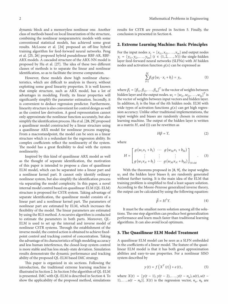
where the activation function Γ(sdot) is chosen as Γ(119909) = 1(1 +
119890minus119909) The whole identification process based on QL-ELM
is described in Figure 1 where 119879(119905) = 1198822Γ(1198821119883(119905) + 119861)
119899119886and 119899
119887are orders of the input and output 119882
1and 119882
2
u(t)
u(t)
middot middot middotmiddot middot middot
y(t)
120579 minus
minus
Γ
Γ Σ
yn(t)W1W2
y(t minus 1)
T(x)
u(t minus na)y(t minus nb)
yl(t)
Nonlinearsystem
ΓX
Figure 1 The process identification based on QL-ELM
are weight matrices of the input and output layer 119861 is biasvector of hidden nodes and 120579 is the parameter of linear partand also can be seen as the bias vector of output nodesThe parameters of two submodels are updated during eachiterative process until the ultimate goal to make the errorbetween the output of actual model and the QL-ELM modelminimized The deviation between 119910(119905) and 119910
119871(119905) is used
to update the nonlinear part through ELM learning Thedeviation between 119910(119905) and 119910
119873(119905) is used to update the linear
part through recursive least squaresThe whole process is to make the error between actual
output and model output minimized In this paper a hierar-chical iterative algorithm is considered for quasilinearmodel
For linear part at every iteration the following RLS isused to minimize the sum of squared residuals 119890 = 119910
119897minus
1199101198972= 119910119897minus 1198831198791205792 avoiding the problems of local optimal
and overfittingFor nonlinear part weights of input layer and biases are
fixed and the training error 119890 = 1198671198822minus 1198792 is minimized
through ELM learning Then the weights of output layer arecalculated as119882
2= 119867dagger119879 The linear parameter 120579 also can be
regarded as noise ELMmethod has capability of interferencesuppression and rapidity Because the linear form of themodel disperses the complexity of the nonlinear processthe computation of nonlinearity estimation can be simplifiedat every iteration It means that less hidden nodes (119872) arerequired to avoid the overfitting problem in some extentUsing the QL-ELM model to identify the reversible modelsystem can improve the identification accuracy and systemperformance
4 IMC with QL-ELM
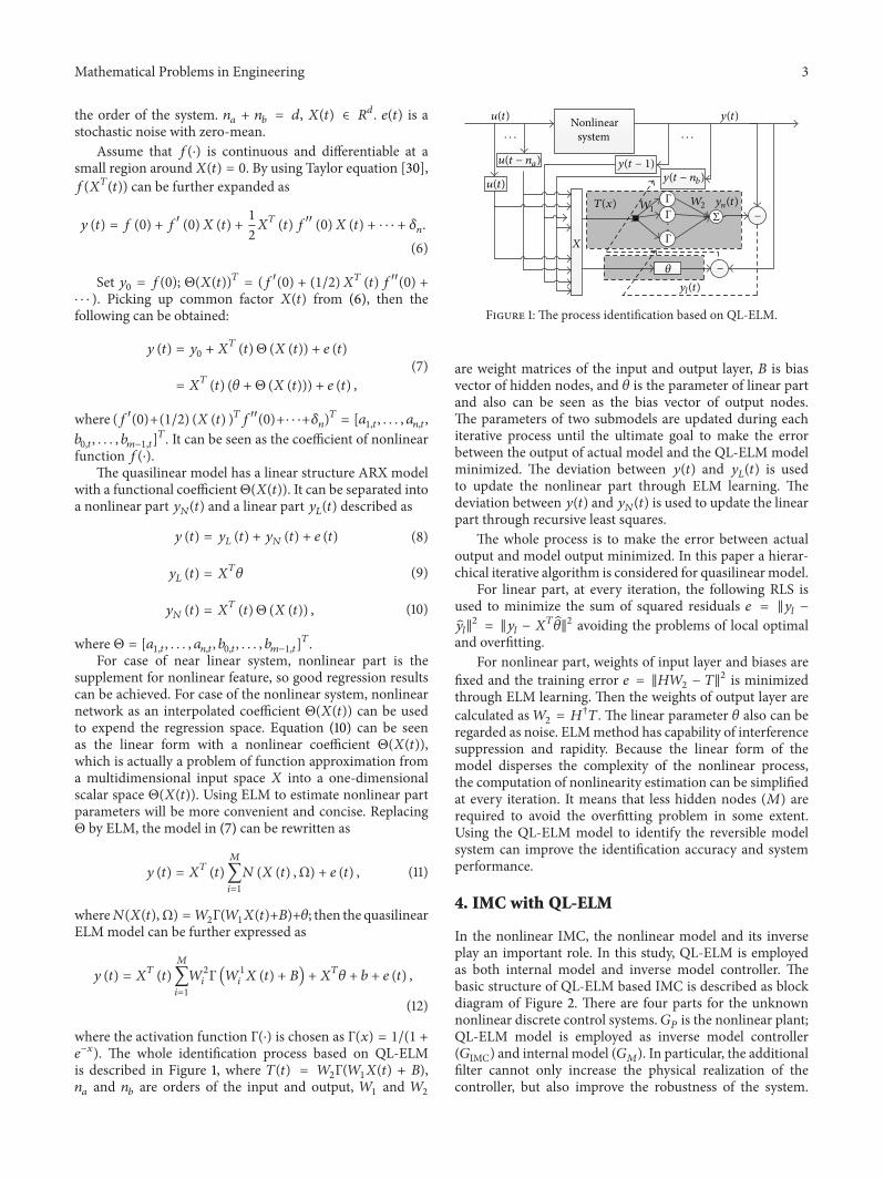
In the nonlinear IMC the nonlinear model and its inverseplay an important role In this study QL-ELM is employedas both internal model and inverse model controller Thebasic structure of QL-ELM based IMC is described as blockdiagram of Figure 2 There are four parts for the unknownnonlinear discrete control systems 119866
119875is the nonlinear plant
QL-ELM model is employed as inverse model controller(119866IMC) and internal model (119866
119872) In particular the additional
filter cannot only increase the physical realization of thecontroller but also improve the robustness of the system
4 Mathematical Problems in Engineering
+minus
minus
y(k)r(k) u(k)QL-ELM
QL-ELMinternal model
inverse model(GIMC )
NonlinearFiltersystem (GP)
(GM)
(Gf)
Figure 2 Structure of IMC system based on QL-ELM
It can effectively solve problems caused by model mismatch[31]
41 Establishment of Internal Model For a nonlinear plantdescribed by
119910 (119896 + 1) = 119891 [119910 (119896) 119910 (119896 minus 1) 119910 (119896 minus 119899119886) 119906 (119896)
119906 (119896 minus 1) 119906 (119896 minus 119899119887)]
(13)
where 119899119886and 119899
119887is the order of output and input vector The
input vector 119909(119896) = [119910(119896) 119910(119896 minus 1) 119910(119896 minus 119899119886) 119906(119896) 119906(119896 minus
1) 119906(119896 minus 119899119887)]119879 and output vector 119910(119896 + 1) are used as
samples to set up the internal model via QL-ELM 119910(119896 +
1) 119909(119896) 119896 isin 1 119873 minus 1 is the training set The learningof QL-ELM is implemented by the following steps
Step 1 (initialization) Choose the order of the regressionvector 119899
119886 119899119887 Set 120579 to zero and the number of nodes in hidden
layer 119872 and nonlinear parameters 1198821 1198822 119861 to some small
values randomly The number of iteration is set to 119899 = 1
Step 2 Update the linear part using deviation 119910119897(119896) = 119910(119896) minus
119910119899(119896) and estimate 120579
119871using (9)
Step 3 Update the nonlinear part using 119910119899(119896) = 119910(119896) minus 119910
119897(119896)
and estimate 120579119873(1198822 119896) using (10)
Step 4 Turn to Step 2 and set 119899 = 119899 + 1 until the trainingerror 119890 = 119884 minus
2 reaches minimum
42 Establishment of Inverse Model The controller of IMCis the inverse model of the nonlinear process which isequivalent to finding the inverse of the system at givenfrequencies Therefore the reversibility of the model must beconsidered in advance
Theorem 1 For the above nonlinear system if the 119909(119896) =
[119910(119896 + 1) 119910(119896) 119910(119896 minus 119899119886) 119906(119896 minus 1) 119906(119896 minus 119899
119887)] is
monotone function to 119906(119896) the system is reversible Or forany given two inputs 119906
1(119896) 119906
2(119896) if 119891(119910(119896) 119910(119896 minus 119899
119906 (119896 minus 1) 119906 (119896 minus 119899119887)]
(14)
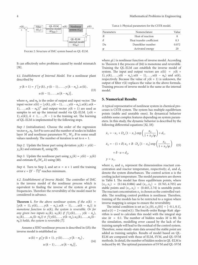
Table 1 Physical parameters for the CSTR model
Parameters Nomenclature Value119861 Heat of reaction 8120575 Heat transfer coefficient 03Da Damokher number 0072120593 Activated energy 20
where 119892(sdot) is nonlinear function of inverse model Accordingto Theorem 1 the process of (14) is monotone and reversibleTraining the QL-ELM can establish the inverse model ofsystem The input and output vectors are 119909(119896) = 119910(119896 +
1) 119910(119896) 119910(119896 minus 119899119886) 119906(119896 minus 1) 119906(119896 minus 119899
119887) and 119906(119896)
respectively Because the value of 119910(119896 + 1) is unknown theoutput of filter 119903(119896) replaces the value in the above formulaTraining process of inverse model is the same as the internalmodel
5 Numerical Results
A typical representative of nonlinear system in chemical pro-cesses is CSTR system The system has multiple equilibriumpoints (stable and unstable ones) Its dynamical behaviorexhibits some complex features depending on system param-eters In this study the dynamic behavior is described by thefollowing differential equations [32 33]
1= minus1199091+ 119863119886(1 minus 119909
1) exp( 119909
2
1 + 1199092120593
) + 1198891
2= minus (1 + 120575) 1199092
+ 119861 sdot 119863119886(1 minus 119909
2) exp( 119909
2
1 + 1199092120593
)
+ 120575 sdot 119906 + 1198892
119910 = 1199091
(15)
where 1199091and 119909
2represent the dimensionless reactant con-
centration and reactor temperature respectively 1198891and 119889
2
denote the system disturbances The control action 119906 is thecooling jacket temperatureThemodel parameters are shownin Table 1 The model has three equilibrium points where(1199091 1199092) = (0144 0886) and (119909
1 1199092) = (0765 4705) are
stable points and (1199091 1199092) = (0445 274) is unstable point
The reactant concentration1199091is chosen as the controlled vari-
able The resulting control problem is nonlinear Thereforetraining of the models has to be restricted to a region whereinverse mapping is unique to ensure the reversibility
The initial condition is set as [1199091(0) 1199092(0)] = [minus01 01]
and 119906 (119905) = 2lowast rand 119899(1) The fourth-order Runge-Kutt algo-rithm is used to calculate this model with the integral stepsize Δ119905 = 01 The number of hidden nodes 119872 is 80 Inthe simulation modelling error caused by the lack of thetraining sample will lead to the residual of the control systemTherefore some steady-state data around the stable point areadded as training samples Results of model based on QL-ELM are compared with those of ELM SVM and QL-SVMmethods In detail the number of hiddennodes inQL-ELM isreduced by 40The optimal parameters of SVM andQL-SVM
Mathematical Problems in Engineering 5
0 50 100 150 200 250 300 350 400 450 500Times
01
012
014
016
018
02
Internal model seriesQL-ELM method
Out
put (
y)
(a) QL-ELMmethod output and the actual output of internal model
0 50 100 150 200 250 300 350 400 450 500Times
Erro
r
0
05
1
15
2
25
3
35
4times10minus3
(b) Error of QL-ELM internal model
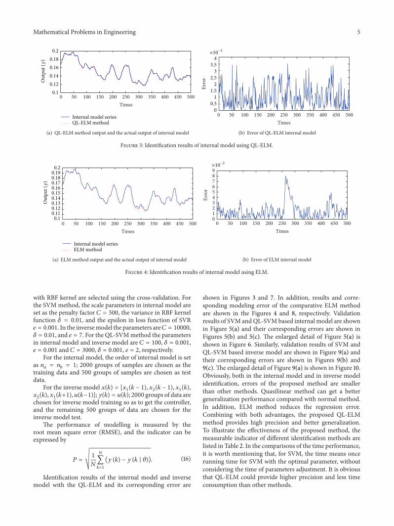
Figure 3 Identification results of internal model using QL-ELM
0 50 100 150 200 250 300 350 400 450 500Times
01
012013
011
014015016017018019
02
Internal model seriesELM method
Out
put (
y)
(a) ELMmethod output and the actual output of internal model
Figure 4 Identification results of internal model using ELM
with RBF kernel are selected using the cross-validation Forthe SVMmethod the scale parameters in internal model areset as the penalty factor 119862 = 500 the variance in RBF kernelfunction 120575 = 001 and the epsilon in loss function of SVR119890 = 0001 In the inversemodel the parameters are119862 = 10000120575 = 001 and 119890 = 7 For the QL-SVMmethod the parametersin internal model and inverse model are 119862 = 100 120575 = 0001119890 = 0001 and 119862 = 3000 120575 = 0001 119890 = 2 respectively
For the internal model the order of internal model is setas 119899119886= 119899119887= 1 2000 groups of samples are chosen as the
training data and 500 groups of samples are chosen as testdata
For the inverse model 119909(119896) = [1199091(119896 minus 1) 119909
2(119896 minus 1) 119909
1(119896)
1199092(119896) 1199091(119896+1) 119906(119896minus1)]119910(119896) = 119906(119896) 2000 groups of data are
chosen for inverse model training so as to get the controllerand the remaining 500 groups of data are chosen for theinverse model test
The performance of modelling is measured by theroot mean square error (RMSE) and the indicator can beexpressed by
119875 = radic1
119873
119873
sum
119896=1
(119910 (119896) minus 119910 (119896 | 120579)) (16)
Identification results of the internal model and inversemodel with the QL-ELM and its corresponding error are
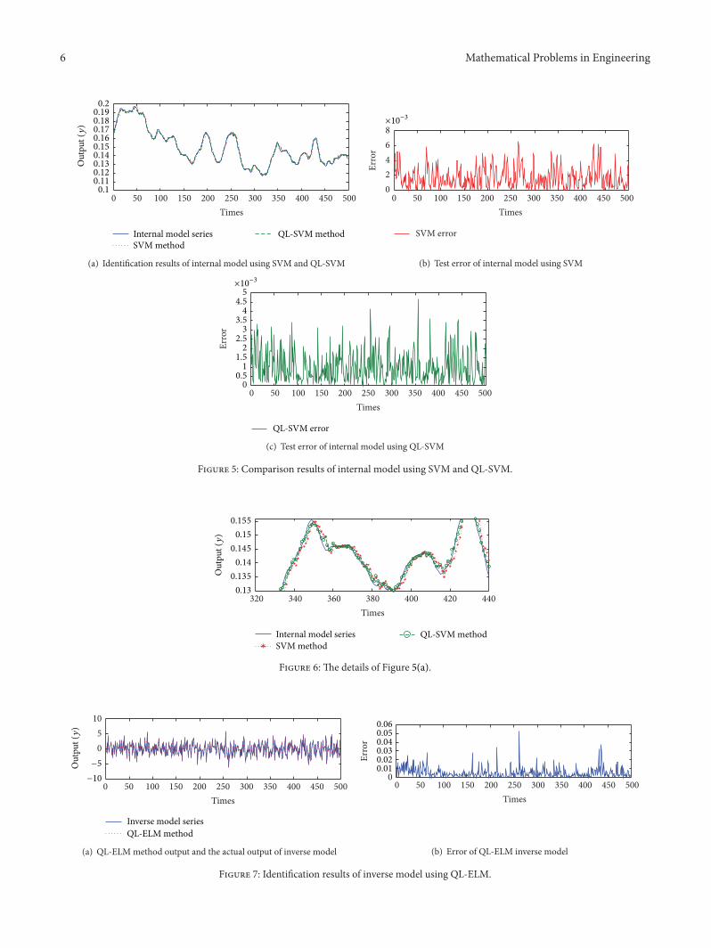
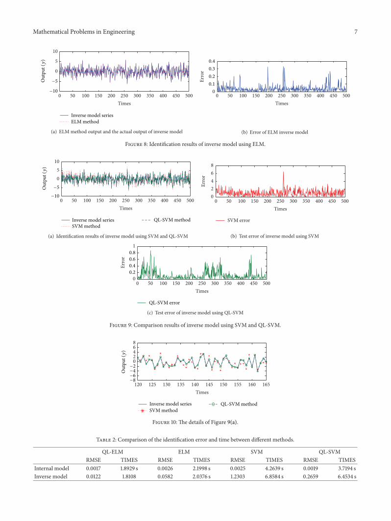
shown in Figures 3 and 7 In addition results and corre-sponding modeling error of the comparative ELM methodare shown in the Figures 4 and 8 respectively Validationresults of SVM andQL-SVMbased internal model are shownin Figure 5(a) and their corresponding errors are shown inFigures 5(b) and 5(c) The enlarged detail of Figure 5(a) isshown in Figure 6 Similarly validation results of SVM andQL-SVM based inverse model are shown in Figure 9(a) andtheir corresponding errors are shown in Figures 9(b) and9(c) The enlarged detail of Figure 9(a) is shown in Figure 10Obviously both in the internal model and in inverse modelidentification errors of the proposed method are smallerthan other methods Quasilinear method can get a bettergeneralization performance compared with normal methodIn addition ELM method reduces the regression errorCombining with both advantages the proposed QL-ELMmethod provides high precision and better generalizationTo illustrate the effectiveness of the proposed method themeasurable indicator of different identification methods arelisted in Table 2 In the comparisons of the time performanceit is worth mentioning that for SVM the time means oncerunning time for SVM with the optimal parameter withoutconsidering the time of parameters adjustment It is obviousthat QL-ELM could provide higher precision and less timeconsumption than other methods
6 Mathematical Problems in Engineering
0 50 100 150 200 250 300 350 400 450 500Times
Internal model seriesSVM method
QL-SVM method
01
012013
011
014015016017018019
02
Out
put (
y)
(a) Identification results of internal model using SVM and QL-SVM
0 50 100 150 200 250 300 350 400 450 50002468
Times
Erro
r
SVM error
times10minus3
(b) Test error of internal model using SVM
0 50 100 150 200 250 300 350 400 450 5000
Times
Erro
r
QL-SVM error
051
152
253
354
455
times10minus3
(c) Test error of internal model using QL-SVM
Figure 5 Comparison results of internal model using SVM and QL-SVM
320 340 360 380 400 420 440Times
013
0135
014
0145
015
0155
Internal model seriesSVM method
QL-SVM method
Out
put (
y)
Figure 6 The details of Figure 5(a)
0 50 100 150 200 250 300 350 400 450 500
05
10
Times
Inverse model seriesQL-ELM method
minus10
minus5Out
put (
y)
(a) QL-ELMmethod output and the actual output of inverse model
0
Erro
r
0 50 100 150 200 250 300 350 400 450 500Times
001002003004005006
(b) Error of QL-ELM inverse model
Figure 7 Identification results of inverse model using QL-ELM
Mathematical Problems in Engineering 7
0 50 100 150 200 250 300 350 400 450 500
0
5
10
Times
minus10
minus5
Inverse model seriesELM method
Out
put (
y)
(a) ELMmethod output and the actual output of inverse model
0
Erro
r
0 50 100 150 200 250 300 350 400 450 500Times
01
02
03
04
(b) Error of ELM inverse model
Figure 8 Identification results of inverse model using ELM
0 50 100 150 200 250 300 350 400 450 500
05
10
Times
minus10
minus5
Inverse model seriesSVM method
QL-SVM method
Out
put (
y)
(a) Identification results of inverse model using SVM and QL-SVM
02468
Erro
r
SVM error
0 50 100 150 200 250 300 350 400 450 500Times
(b) Test error of inverse model using SVM
0
1
Erro
r
0 50 100 150 200 250 300 350 400 450 500Times
QL-SVM error
02
04
06
08
(c) Test error of inverse model using QL-SVM
Figure 9 Comparison results of inverse model using SVM and QL-SVM
120 125 130 135 140 145 150 155 160 165
02468
Times
Inverse model seriesSVM method
QL-SVM method
minus2minus4minus6minus8
Out
put (
y)
Figure 10 The details of Figure 9(a)
Table 2 Comparison of the identification error and time between different methods
QL-ELM ELM SVM QL-SVMRMSE TIMES RMSE TIMES RMSE TIMES RMSE TIMES
Internal model 00017 18929 s 00026 21998 s 00025 42639 s 00019 37194 sInverse model 00122 18108 00582 20376 s 12303 68584 s 02659 64534 s
8 Mathematical Problems in Engineering
0 500 1000 1500 2000 25000105
0110115
0120125
0130135
0140145
Samples
QL-ELM-IMCELM-IMC
SVM-ELMr
Out
put (
y)
(a) Control output using IMC based on QL-ELM ELM and SVM
0 500 1000 1500 2000 2500
00005
0010015
Samples
Erro
r
minus0015minus001
minus0005
QL-ELM-IMCELM-IMC
SVM-ELM
(b) Error of output using IMC based on QL-ELM ELM and SVM
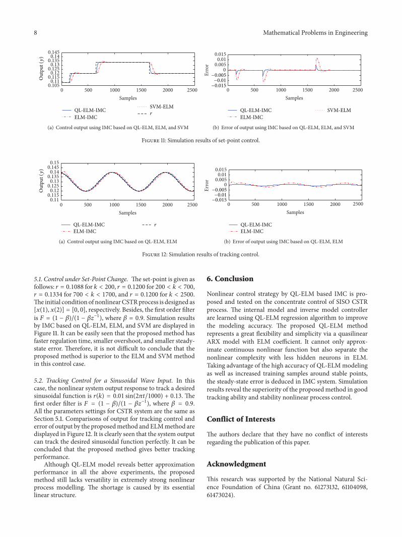
Figure 11 Simulation results of set-point control
0 500 1000 1500 2000 2500011
0115012
0125013
0135014
0145015
Samples
QL-ELM-IMCELM-IMC
r
Out
put (
y)
(a) Control output using IMC based on QL-ELM ELM
0 500 1000 1500 2000 2500
00005
0010015
SamplesEr
ror
QL-ELM-IMCELM-IMC
minus0015minus001
minus0005
(b) Error of output using IMC based on QL-ELM ELM
Figure 12 Simulation results of tracking control
51 Control under Set-Point Change The set-point is given asfollows 119903 = 01088 for 119896 lt 200 119903 = 01200 for 200 lt 119896 lt 700119903 = 01334 for 700 lt 119896 lt 1700 and 119903 = 01200 for 119896 lt 2500The initial condition of nonlinearCSTRprocess is designed as[119909(1) 119909(2)] = [0 0] respectively Besides the first order filteris 119865 = (1 minus 120573)(1 minus 120573119911
minus1) where 120573 = 09 Simulation results
by IMC based on QL-ELM ELM and SVM are displayed inFigure 11 It can be easily seen that the proposed method hasfaster regulation time smaller overshoot and smaller steady-state error Therefore it is not difficult to conclude that theproposed method is superior to the ELM and SVM methodin this control case
52 Tracking Control for a Sinusoidal Wave Input In thiscase the nonlinear system output response to track a desiredsinusoidal function is 119903(119896) = 001 sin(21205871199051000) + 013 Thefirst order filter is 119865 = (1 minus 120573)(1 minus 120573119911
minus1) where 120573 = 09
All the parameters settings for CSTR system are the same asSection 51 Comparisons of output for tracking control anderror of output by the proposedmethod and ELMmethod aredisplayed in Figure 12 It is clearly seen that the system outputcan track the desired sinusoidal function perfectly It can beconcluded that the proposed method gives better trackingperformance
Although QL-ELM model reveals better approximationperformance in all the above experiments the proposedmethod still lacks versatility in extremely strong nonlinearprocess modelling The shortage is caused by its essentiallinear structure
6 Conclusion
Nonlinear control strategy by QL-ELM based IMC is pro-posed and tested on the concentrate control of SISO CSTRprocess The internal model and inverse model controllerare learned using QL-ELM regression algorithm to improvethe modeling accuracy The proposed QL-ELM methodrepresents a great flexibility and simplicity via a quasilinearARX model with ELM coefficient It cannot only approx-imate continuous nonlinear function but also separate thenonlinear complexity with less hidden neurons in ELMTaking advantage of the high accuracy of QL-ELMmodelingas well as increased training samples around stable pointsthe steady-state error is deduced in IMC system Simulationresults reveal the superiority of the proposedmethod in goodtracking ability and stability nonlinear process control
Conflict of Interests
The authors declare that they have no conflict of interestsregarding the publication of this paper
Acknowledgment
This research was supported by the National Natural Sci-ence Foundation of China (Grant no 61273132 6110409861473024)
Mathematical Problems in Engineering 9
References
[1] H Deng and H-X Li ldquoA novel neural approximate inversecontrol for unknown nonlinear discrete dynamical systemsrdquoIEEE Transactions on Systems Man and Cybernetics Part BCybernetics vol 35 no 1 pp 115ndash123 2005
[2] H Yu H R Karimi and X Zhu ldquoResearch of smart carrsquosspeed control based on the internalmodel controlrdquoAbstract andApplied Analysis vol 2014 Article ID 274293 5 pages 2014
[3] I Rivals and L Personnaz ldquoNonlinear internal model controlusing neural networks application to processes with delay anddesign issuesrdquo IEEETransactions onNeural Networks vol 11 no1 pp 80ndash90 2000
[4] Y-N Wang and X-F Yuan ldquoSVM approximate-based internalmodel control strategyrdquo Acta Automatica Sinica vol 34 no 2pp 172ndash179 2008
[5] I Rivals and L Personnaz ldquoNonlinear internal model controlusing neural networks application to processes with delay anddesign issuesrdquo IEEETransactions onNeural Networks vol 11 no1 pp 80ndash90 2000
[6] H-X Li and H Deng ldquoAn approximate internal model-basedneural control for unknown nonlinear discrete processesrdquo IEEETransactions on Neural Networks vol 17 no 3 pp 659ndash6702006
[7] Y Huang and D Wu ldquoNonlinear internal model control withinverse model based on extreme learning machinerdquo in Proceed-ings of the International Conference on Electric Information andControl Engineering (ICEICE rsquo11) pp 2391ndash2395Wuhan ChinaApril 2011
[8] G-B Huang Q-Y Zhu and C-K Siew ldquoExtreme learningmachine theory and applicationsrdquoNeurocomputing vol 70 no1ndash3 pp 489ndash501 2006
[9] G-B Huang and L Chen ldquoConvex incremental extreme learn-ing machinerdquo Neurocomputing vol 70 no 16ndash18 pp 3056ndash3062 2007
[10] G-B Huang and L Chen ldquoEnhanced random search basedincremental extreme learning machinerdquo Neurocomputing vol71 no 16ndash18 pp 3460ndash3468 2008
[11] Y Song and J Zhang ldquoAutomatic recognition of epileptic EEGpatterns via Extreme Learning Machine and multiresolutionfeature extractionrdquoExpert Systemswith Applications vol 40 no14 pp 5477ndash5489 2013
[12] Y Chen Z Zhao S Wang and Z Chen ldquoExtreme learningmachine-based device displacement free activity recognitionmodelrdquo Soft Computing vol 16 no 9 pp 1617ndash1625 2012
[13] J Cao T Chen and J Fan ldquoFast online learning algorithm forlandmark recognition based on BoW frameworkrdquo in Proceed-ings of the 9th IEEE Conference on Industrial Electronics andApplications pp 1163ndash1168 2014
[14] P K Wong Z Yang C M Vong and J Zhong ldquoReal-timefault diagnosis for gas turbine generator systems using extremelearning machinerdquoNeurocomputing vol 128 pp 249ndash257 2014
[15] G Wang Y Zhao and D Wang ldquoA protein secondary struc-ture prediction framework based on the Extreme LearningMachinerdquo Neurocomputing vol 72 no 1ndash3 pp 262ndash268 2008
[16] R K Pearson and B A Ogunnaike Identification and ControlUsing Volterra Models Springer 2002
[17] K T Iskakov and Z O Oralbekova ldquoResolving power ofalgorithm for solving the coefficient inverse problem for thegeoelectric equationrdquo Mathematical Problems in Engineeringvol 2014 Article ID 545689 9 pages 2014
[18] S I Biagiola and J L Figueroa ldquoIdentification of uncertainMIMOWiener andHammersteinmodelsrdquoComputersampChem-ical Engineering vol 35 no 12 pp 2867ndash2875 2011
[19] Y Tang Z Li and X Guan ldquoIdentification of nonlinearsystem using extreme learning machine based Hammersteinmodelrdquo Communications in Nonlinear Science and NumericalSimulation vol 19 no 9 pp 3171ndash3183 2014
[20] A Wills T B Schon L Ljung and B Ninness ldquoIdentificationof Hammerstein-Wiener modelsrdquo Automatica vol 49 no 1 pp70ndash81 2013
[21] D Wang and F Ding ldquoExtended stochastic gradient identifi-cation algorithms for Hammerstein-Wiener ARMAX systemsrdquoComputers amp Mathematics with Applications vol 56 no 12 pp3157ndash3164 2008
[22] J G Smith S Kamat and K P Madhavan ldquoModeling of pHprocess using wavenet based Hammerstein modelrdquo Journal ofProcess Control vol 17 no 6 pp 551ndash561 2007
[23] L Zhou X Li and F Pan ldquoGradient-based iterative identifi-cation for MISO Wiener nonlinear systems application to aglutamate fermentation processrdquo Applied Mathematics Lettersvol 26 no 8 pp 886ndash892 2013
[24] S McLoone M D Brown G Irwin and G Lightbody ldquoAhybrid linearnonlinear training algorithm for feedforwardneural networksrdquo IEEE Transactions on Neural Networks vol9 no 4 pp 669ndash684 1998
[25] H Peng T Ozaki V Haggan-Ozaki and Y Toyoda ldquoA parame-ter optimization method for radial basis function type modelsrdquoIEEE Transactions on Neural Networks vol 14 no 2 pp 432ndash438 2003
[26] H Peng T Ozaki Y Toyoda et al ldquoRBF-ARX model-basednonlinear system modeling and predictive control with appli-cation to a NOx decomposition processrdquo Control EngineeringPractice vol 12 no 2 pp 191ndash203 2004
[27] B Hu Z Zhao and J Liang ldquoMulti-loop nonlinear internalmodel controller design under nonlinear dynamic PLS frame-work using ARX-neural network modelrdquo Journal of ProcessControl vol 22 no 1 pp 207ndash217 2012
[28] J Hu K Kumamaru and K Inoue ldquoA hybrid quasi-ARMAXmodeling scheme for identification of nonlinear systemsrdquoTransactions of the Society of Instrument and Control Engineersvol 34 no 8 pp 977ndash985 1998
[29] Y Cheng and J Hu ldquoNonlinear system identification basedon SVR with quasi-linear kernelrdquo in Proceedings of the AnnualInternational Joint Conference on Neural Networks (IJCNN rsquo12)pp 1ndash8 June 2012
[30] G Prasad E Swidenbank and B W Hogg ldquoA local modelnetworks based multivariable long-range predictive controlstrategy for thermal power plantsrdquo Automatica vol 34 no 10pp 1185ndash1204 1998
[31] Y Zhang and Z Zheng ldquoBased on inverse system of internalmodel controlrdquo in Proceedings of the International Conferenceon Computer Application and System Modeling (ICCASM rsquo10)pp V14ndash19ndashV14ndash21 Taiyuan China October 2010
[32] C-T Chen and S-T Peng ldquoIntelligent process control usingneural fuzzy techniquesrdquo Journal of Process Control vol 9 no6 pp 493ndash503 1999
[33] C-T Chen and S-T Peng ldquoLearning control of process systemswith hard input constraintsrdquo Journal of Process Control vol 9no 2 pp 151ndash160 1999
dynamic block and a memoryless nonlinear one Anotherclass of methods based on local linearization of the structurecombining the nonlinear nonparametric models with someconventional statistical models has achieved some greatresults McLoone et al [24] proposed an off-line hybridtraining algorithm for feed-forward neural networks Penget al [25 26] proposed hybrid pseudolinear RBF-AR RBF-ARX models A cascaded structure of the ARX-NN model isproposed by Hu et al [27] The idea of these two differentclasses of methods is to separate the linear and nonlinearidentification so as to facilitate the inverse computation
However these models show high nonlinear charac-teristics which are difficult to analysis in theory withoutexploiting some good linearity properties It is well knownthat simple structure such as ARX model has a lot ofadvantages in modeling Firstly its linear properties willsignificantly simplify the parameter estimation Secondly itis convenient to deduce regression predictor Furthermorelinearity structure is also convenient for control design as wellas the control law derivation A good representation cannotonly approximate the nonlinear function accurately but alsosimplify the identification process Hu et al [28 29] proposeda quasilinear model constructed by a linear structure usinga quasilinear ARX model for nonlinear process mappingFrom a macrostandpoint the model can be seen as a linearstructure which is a redundant for the regression ability Itscomplex coefficients reflect the nonlinearity of the systemThe model has a great flexibility to deal with the systemnonlinearity
Inspired by this kind of quasilinear ARX model as wellas the thought of separate identification the motivationof this paper is intended to propose a class of quasilinearELM model which can be separated into a linear part anda nonlinear kernel part It cannot only identify ordinarynonlinear system but also simplify the identification processvia separating the model complexity In this paper a novelinternal model control based on quasilinear-ELM (QL-ELM)structure is proposed for CSTR system Taking advantage ofseparate identification the quasilinear model consists of alinear part and a nonlinear kernel part The parameters ofnonlinear part are estimated by ELM which increases theflexibility of the model The linear parameters are estimatedby using the RLSmethod A recursive algorithm is conductedto estimate the parameters in both parts Moreover QL-ELM is used to set up the internal and inverse model ofnonlinear CSTR systems Through the establishment of theinversemodel the control action is obtained to achieve fixed-point control and tracking control of concentration Takingthe advantage of its characteristics of highmodeling accuracyand less human interference the closed-loop system controlis more stable and has less steady-state deviation Simulationresults demonstrate the dynamic performance and trackingability of the proposed QL-ELM based IMC strategy
This paper is organized in six sections Following theintroduction the traditional extreme learning machine isillustrated in Section 2 In Section 3 the algorithmofQL-ELMis presented IMC with QL-ELM is described in Section 4 Toshow the applicability of the proposed method simulations
results for CSTR are presented in Section 5 Finally theconclusion is presented in Section 6
2 Extreme Learning Machine Basic Principles
For the input nodes 119909119894= [1199091198941 1199091198942 119909
119894119899] and output nodes
119910119894= [1199101198941 1199101198942 119910
119894119898] (119894 isin (1 2 119873)) the single-hidden
layer feed-forward neural networks (SLFNs) with119872 hiddennodes and activation function 119892(119909) can be expressed as
119894119899]119879 is the vector of weights between
hidden layer and the output nodes119908119894= [1199081198941 1199081198942 119908
119894119899]119879 is
the vector of weights between input vectors and hidden layerIn addition 119887
119894is the bias of the 119894th hidden node ELM with
wide types of activation functions 119892(119909) can get high regres-sion accuracy Unlike other traditional implementations theinput weights and biases are randomly chosen in extremelearning machine The output of the hidden layer is writtenas a matrix119867 and (1) can be rewritten as
With the theorems proposed in [8 9] the input weights119908119894and the hidden layer biases 119887
119894are randomly generated
without further tuning It is the main idea of the ELM thattraining problem is simplified to find a least square solutionAccording to the Moore-Penrose generalized inverse theorythe output can be calculated by using the following equation
120573 = 119867
dagger119884 (4)
It must be the smallest norm solution among all the solu-tionsThe one step algorithm can produce best generalizationperformance and learn much faster than traditional learningalgorithms It can also avoid local optimum
3 The Quasilinear ELM Model Treatment
A quasilinear ELM model can be seen as a SLFN embeddedin the coefficients of a linear model The feature of the quasi-linear ELM model is that it has both good approximationabilities and easy-to-use properties For a nonlinear SISOsystem described by
where 119883(119905) = [119910(119905 minus 1) 119910(119905 minus 2) 119910(119905 minus 119899119886) 119906(119905) 119906(119905 minus
1) 119906(119905 minus 119899119887)] 119883(119905) is the regression vector 119899
119886 119899119887are
Mathematical Problems in Engineering 3
the order of the system 119899119886+ 119899119887= 119889 119883(119905) isin 119877
119889 119890(119905) is astochastic noise with zero-mean
Assume that 119891(sdot) is continuous and differentiable at asmall region around119883(119905) = 0 By using Taylor equation [30]119891(119883119879(119905)) can be further expanded as
For case of near linear system nonlinear part is thesupplement for nonlinear feature so good regression resultscan be achieved For case of the nonlinear system nonlinearnetwork as an interpolated coefficient Θ(119883(119905)) can be usedto expend the regression space Equation (10) can be seenas the linear form with a nonlinear coefficient Θ(119883(119905))which is actually a problem of function approximation froma multidimensional input space 119883 into a one-dimensionalscalar space Θ(119883(119905)) Using ELM to estimate nonlinear partparameters will be more convenient and concise ReplacingΘ by ELM the model in (7) can be rewritten as
119910 (119905) = 119883119879(119905)
119872
sum
119894=1
119873(119883 (119905) Ω) + 119890 (119905) (11)
where119873(119883(119905) Ω) = 1198822Γ(1198821119883(119905)+119861)+120579 then the quasilinear
ELMmodel can be further expressed as
119910 (119905) = 119883119879(119905)
119872
sum
119894=1
1198822
119894Γ (1198821
119894119883 (119905) + 119861) + 119883
119879120579 + 119887 + 119890 (119905)
(12)
where the activation function Γ(sdot) is chosen as Γ(119909) = 1(1 +
119890minus119909) The whole identification process based on QL-ELM
is described in Figure 1 where 119879(119905) = 1198822Γ(1198821119883(119905) + 119861)
119899119886and 119899
119887are orders of the input and output 119882
1and 119882
2
u(t)
u(t)
middot middot middotmiddot middot middot
y(t)
120579 minus
minus
Γ
Γ Σ
yn(t)W1W2
y(t minus 1)
T(x)
u(t minus na)y(t minus nb)
yl(t)
Nonlinearsystem
ΓX
Figure 1 The process identification based on QL-ELM
are weight matrices of the input and output layer 119861 is biasvector of hidden nodes and 120579 is the parameter of linear partand also can be seen as the bias vector of output nodesThe parameters of two submodels are updated during eachiterative process until the ultimate goal to make the errorbetween the output of actual model and the QL-ELM modelminimized The deviation between 119910(119905) and 119910
119871(119905) is used
to update the nonlinear part through ELM learning Thedeviation between 119910(119905) and 119910
119873(119905) is used to update the linear
part through recursive least squaresThe whole process is to make the error between actual
output and model output minimized In this paper a hierar-chical iterative algorithm is considered for quasilinearmodel
For linear part at every iteration the following RLS isused to minimize the sum of squared residuals 119890 = 119910
119897minus
1199101198972= 119910119897minus 1198831198791205792 avoiding the problems of local optimal
and overfittingFor nonlinear part weights of input layer and biases are
fixed and the training error 119890 = 1198671198822minus 1198792 is minimized
through ELM learning Then the weights of output layer arecalculated as119882
2= 119867dagger119879 The linear parameter 120579 also can be
regarded as noise ELMmethod has capability of interferencesuppression and rapidity Because the linear form of themodel disperses the complexity of the nonlinear processthe computation of nonlinearity estimation can be simplifiedat every iteration It means that less hidden nodes (119872) arerequired to avoid the overfitting problem in some extentUsing the QL-ELM model to identify the reversible modelsystem can improve the identification accuracy and systemperformance
4 IMC with QL-ELM
In the nonlinear IMC the nonlinear model and its inverseplay an important role In this study QL-ELM is employedas both internal model and inverse model controller Thebasic structure of QL-ELM based IMC is described as blockdiagram of Figure 2 There are four parts for the unknownnonlinear discrete control systems 119866
119875is the nonlinear plant
QL-ELM model is employed as inverse model controller(119866IMC) and internal model (119866
119872) In particular the additional
filter cannot only increase the physical realization of thecontroller but also improve the robustness of the system
4 Mathematical Problems in Engineering
+minus
minus
y(k)r(k) u(k)QL-ELM
QL-ELMinternal model
inverse model(GIMC )
NonlinearFiltersystem (GP)
(GM)
(Gf)
Figure 2 Structure of IMC system based on QL-ELM
It can effectively solve problems caused by model mismatch[31]
41 Establishment of Internal Model For a nonlinear plantdescribed by
119910 (119896 + 1) = 119891 [119910 (119896) 119910 (119896 minus 1) 119910 (119896 minus 119899119886) 119906 (119896)
119906 (119896 minus 1) 119906 (119896 minus 119899119887)]
(13)
where 119899119886and 119899
119887is the order of output and input vector The
input vector 119909(119896) = [119910(119896) 119910(119896 minus 1) 119910(119896 minus 119899119886) 119906(119896) 119906(119896 minus
1) 119906(119896 minus 119899119887)]119879 and output vector 119910(119896 + 1) are used as
samples to set up the internal model via QL-ELM 119910(119896 +
1) 119909(119896) 119896 isin 1 119873 minus 1 is the training set The learningof QL-ELM is implemented by the following steps
Step 1 (initialization) Choose the order of the regressionvector 119899
119886 119899119887 Set 120579 to zero and the number of nodes in hidden
layer 119872 and nonlinear parameters 1198821 1198822 119861 to some small
values randomly The number of iteration is set to 119899 = 1
Step 2 Update the linear part using deviation 119910119897(119896) = 119910(119896) minus
119910119899(119896) and estimate 120579
119871using (9)
Step 3 Update the nonlinear part using 119910119899(119896) = 119910(119896) minus 119910
119897(119896)
and estimate 120579119873(1198822 119896) using (10)
Step 4 Turn to Step 2 and set 119899 = 119899 + 1 until the trainingerror 119890 = 119884 minus
2 reaches minimum
42 Establishment of Inverse Model The controller of IMCis the inverse model of the nonlinear process which isequivalent to finding the inverse of the system at givenfrequencies Therefore the reversibility of the model must beconsidered in advance
Theorem 1 For the above nonlinear system if the 119909(119896) =
[119910(119896 + 1) 119910(119896) 119910(119896 minus 119899119886) 119906(119896 minus 1) 119906(119896 minus 119899
119887)] is
monotone function to 119906(119896) the system is reversible Or forany given two inputs 119906
1(119896) 119906
2(119896) if 119891(119910(119896) 119910(119896 minus 119899
119906 (119896 minus 1) 119906 (119896 minus 119899119887)]
(14)
Table 1 Physical parameters for the CSTR model
Parameters Nomenclature Value119861 Heat of reaction 8120575 Heat transfer coefficient 03Da Damokher number 0072120593 Activated energy 20
where 119892(sdot) is nonlinear function of inverse model Accordingto Theorem 1 the process of (14) is monotone and reversibleTraining the QL-ELM can establish the inverse model ofsystem The input and output vectors are 119909(119896) = 119910(119896 +
1) 119910(119896) 119910(119896 minus 119899119886) 119906(119896 minus 1) 119906(119896 minus 119899
119887) and 119906(119896)
respectively Because the value of 119910(119896 + 1) is unknown theoutput of filter 119903(119896) replaces the value in the above formulaTraining process of inverse model is the same as the internalmodel
5 Numerical Results
A typical representative of nonlinear system in chemical pro-cesses is CSTR system The system has multiple equilibriumpoints (stable and unstable ones) Its dynamical behaviorexhibits some complex features depending on system param-eters In this study the dynamic behavior is described by thefollowing differential equations [32 33]
1= minus1199091+ 119863119886(1 minus 119909
1) exp( 119909
2
1 + 1199092120593
) + 1198891
2= minus (1 + 120575) 1199092
+ 119861 sdot 119863119886(1 minus 119909
2) exp( 119909
2
1 + 1199092120593
)
+ 120575 sdot 119906 + 1198892
119910 = 1199091
(15)
where 1199091and 119909
2represent the dimensionless reactant con-
centration and reactor temperature respectively 1198891and 119889
2
denote the system disturbances The control action 119906 is thecooling jacket temperatureThemodel parameters are shownin Table 1 The model has three equilibrium points where(1199091 1199092) = (0144 0886) and (119909
1 1199092) = (0765 4705) are
stable points and (1199091 1199092) = (0445 274) is unstable point
The reactant concentration1199091is chosen as the controlled vari-
able The resulting control problem is nonlinear Thereforetraining of the models has to be restricted to a region whereinverse mapping is unique to ensure the reversibility
The initial condition is set as [1199091(0) 1199092(0)] = [minus01 01]
and 119906 (119905) = 2lowast rand 119899(1) The fourth-order Runge-Kutt algo-rithm is used to calculate this model with the integral stepsize Δ119905 = 01 The number of hidden nodes 119872 is 80 Inthe simulation modelling error caused by the lack of thetraining sample will lead to the residual of the control systemTherefore some steady-state data around the stable point areadded as training samples Results of model based on QL-ELM are compared with those of ELM SVM and QL-SVMmethods In detail the number of hiddennodes inQL-ELM isreduced by 40The optimal parameters of SVM andQL-SVM
Mathematical Problems in Engineering 5
0 50 100 150 200 250 300 350 400 450 500Times
01
012
014
016
018
02
Internal model seriesQL-ELM method
Out
put (
y)
(a) QL-ELMmethod output and the actual output of internal model
0 50 100 150 200 250 300 350 400 450 500Times
Erro
r
0
05
1
15
2
25
3
35
4times10minus3
(b) Error of QL-ELM internal model
Figure 3 Identification results of internal model using QL-ELM
0 50 100 150 200 250 300 350 400 450 500Times
01
012013
011
014015016017018019
02
Internal model seriesELM method
Out
put (
y)
(a) ELMmethod output and the actual output of internal model
Figure 4 Identification results of internal model using ELM
with RBF kernel are selected using the cross-validation Forthe SVMmethod the scale parameters in internal model areset as the penalty factor 119862 = 500 the variance in RBF kernelfunction 120575 = 001 and the epsilon in loss function of SVR119890 = 0001 In the inversemodel the parameters are119862 = 10000120575 = 001 and 119890 = 7 For the QL-SVMmethod the parametersin internal model and inverse model are 119862 = 100 120575 = 0001119890 = 0001 and 119862 = 3000 120575 = 0001 119890 = 2 respectively
For the internal model the order of internal model is setas 119899119886= 119899119887= 1 2000 groups of samples are chosen as the
training data and 500 groups of samples are chosen as testdata
For the inverse model 119909(119896) = [1199091(119896 minus 1) 119909
2(119896 minus 1) 119909
1(119896)
1199092(119896) 1199091(119896+1) 119906(119896minus1)]119910(119896) = 119906(119896) 2000 groups of data are
chosen for inverse model training so as to get the controllerand the remaining 500 groups of data are chosen for theinverse model test
The performance of modelling is measured by theroot mean square error (RMSE) and the indicator can beexpressed by
119875 = radic1
119873
119873
sum
119896=1
(119910 (119896) minus 119910 (119896 | 120579)) (16)
Identification results of the internal model and inversemodel with the QL-ELM and its corresponding error are
shown in Figures 3 and 7 In addition results and corre-sponding modeling error of the comparative ELM methodare shown in the Figures 4 and 8 respectively Validationresults of SVM andQL-SVMbased internal model are shownin Figure 5(a) and their corresponding errors are shown inFigures 5(b) and 5(c) The enlarged detail of Figure 5(a) isshown in Figure 6 Similarly validation results of SVM andQL-SVM based inverse model are shown in Figure 9(a) andtheir corresponding errors are shown in Figures 9(b) and9(c) The enlarged detail of Figure 9(a) is shown in Figure 10Obviously both in the internal model and in inverse modelidentification errors of the proposed method are smallerthan other methods Quasilinear method can get a bettergeneralization performance compared with normal methodIn addition ELM method reduces the regression errorCombining with both advantages the proposed QL-ELMmethod provides high precision and better generalizationTo illustrate the effectiveness of the proposed method themeasurable indicator of different identification methods arelisted in Table 2 In the comparisons of the time performanceit is worth mentioning that for SVM the time means oncerunning time for SVM with the optimal parameter withoutconsidering the time of parameters adjustment It is obviousthat QL-ELM could provide higher precision and less timeconsumption than other methods
6 Mathematical Problems in Engineering
0 50 100 150 200 250 300 350 400 450 500Times
Internal model seriesSVM method
QL-SVM method
01
012013
011
014015016017018019
02
Out
put (
y)
(a) Identification results of internal model using SVM and QL-SVM
0 50 100 150 200 250 300 350 400 450 50002468
Times
Erro
r
SVM error
times10minus3
(b) Test error of internal model using SVM
0 50 100 150 200 250 300 350 400 450 5000
Times
Erro
r
QL-SVM error
051
152
253
354
455
times10minus3
(c) Test error of internal model using QL-SVM
Figure 5 Comparison results of internal model using SVM and QL-SVM
320 340 360 380 400 420 440Times
013
0135
014
0145
015
0155
Internal model seriesSVM method
QL-SVM method
Out
put (
y)
Figure 6 The details of Figure 5(a)
0 50 100 150 200 250 300 350 400 450 500
05
10
Times
Inverse model seriesQL-ELM method
minus10
minus5Out
put (
y)
(a) QL-ELMmethod output and the actual output of inverse model
0
Erro
r
0 50 100 150 200 250 300 350 400 450 500Times
001002003004005006
(b) Error of QL-ELM inverse model
Figure 7 Identification results of inverse model using QL-ELM
Mathematical Problems in Engineering 7
0 50 100 150 200 250 300 350 400 450 500
0
5
10
Times
minus10
minus5
Inverse model seriesELM method
Out
put (
y)
(a) ELMmethod output and the actual output of inverse model
0
Erro
r
0 50 100 150 200 250 300 350 400 450 500Times
01
02
03
04
(b) Error of ELM inverse model
Figure 8 Identification results of inverse model using ELM
0 50 100 150 200 250 300 350 400 450 500
05
10
Times
minus10
minus5
Inverse model seriesSVM method
QL-SVM method
Out
put (
y)
(a) Identification results of inverse model using SVM and QL-SVM
02468
Erro
r
SVM error
0 50 100 150 200 250 300 350 400 450 500Times
(b) Test error of inverse model using SVM
0
1
Erro
r
0 50 100 150 200 250 300 350 400 450 500Times
QL-SVM error
02
04
06
08
(c) Test error of inverse model using QL-SVM
Figure 9 Comparison results of inverse model using SVM and QL-SVM
120 125 130 135 140 145 150 155 160 165
02468
Times
Inverse model seriesSVM method
QL-SVM method
minus2minus4minus6minus8
Out
put (
y)
Figure 10 The details of Figure 9(a)
Table 2 Comparison of the identification error and time between different methods
QL-ELM ELM SVM QL-SVMRMSE TIMES RMSE TIMES RMSE TIMES RMSE TIMES
Internal model 00017 18929 s 00026 21998 s 00025 42639 s 00019 37194 sInverse model 00122 18108 00582 20376 s 12303 68584 s 02659 64534 s
8 Mathematical Problems in Engineering
0 500 1000 1500 2000 25000105
0110115
0120125
0130135
0140145
Samples
QL-ELM-IMCELM-IMC
SVM-ELMr
Out
put (
y)
(a) Control output using IMC based on QL-ELM ELM and SVM
0 500 1000 1500 2000 2500
00005
0010015
Samples
Erro
r
minus0015minus001
minus0005
QL-ELM-IMCELM-IMC
SVM-ELM
(b) Error of output using IMC based on QL-ELM ELM and SVM
Figure 11 Simulation results of set-point control
0 500 1000 1500 2000 2500011
0115012
0125013
0135014
0145015
Samples
QL-ELM-IMCELM-IMC
r
Out
put (
y)
(a) Control output using IMC based on QL-ELM ELM
0 500 1000 1500 2000 2500
00005
0010015
SamplesEr
ror
QL-ELM-IMCELM-IMC
minus0015minus001
minus0005
(b) Error of output using IMC based on QL-ELM ELM
Figure 12 Simulation results of tracking control
51 Control under Set-Point Change The set-point is given asfollows 119903 = 01088 for 119896 lt 200 119903 = 01200 for 200 lt 119896 lt 700119903 = 01334 for 700 lt 119896 lt 1700 and 119903 = 01200 for 119896 lt 2500The initial condition of nonlinearCSTRprocess is designed as[119909(1) 119909(2)] = [0 0] respectively Besides the first order filteris 119865 = (1 minus 120573)(1 minus 120573119911
minus1) where 120573 = 09 Simulation results
by IMC based on QL-ELM ELM and SVM are displayed inFigure 11 It can be easily seen that the proposed method hasfaster regulation time smaller overshoot and smaller steady-state error Therefore it is not difficult to conclude that theproposed method is superior to the ELM and SVM methodin this control case
52 Tracking Control for a Sinusoidal Wave Input In thiscase the nonlinear system output response to track a desiredsinusoidal function is 119903(119896) = 001 sin(21205871199051000) + 013 Thefirst order filter is 119865 = (1 minus 120573)(1 minus 120573119911
minus1) where 120573 = 09
All the parameters settings for CSTR system are the same asSection 51 Comparisons of output for tracking control anderror of output by the proposedmethod and ELMmethod aredisplayed in Figure 12 It is clearly seen that the system outputcan track the desired sinusoidal function perfectly It can beconcluded that the proposed method gives better trackingperformance
Although QL-ELM model reveals better approximationperformance in all the above experiments the proposedmethod still lacks versatility in extremely strong nonlinearprocess modelling The shortage is caused by its essentiallinear structure
6 Conclusion
Nonlinear control strategy by QL-ELM based IMC is pro-posed and tested on the concentrate control of SISO CSTRprocess The internal model and inverse model controllerare learned using QL-ELM regression algorithm to improvethe modeling accuracy The proposed QL-ELM methodrepresents a great flexibility and simplicity via a quasilinearARX model with ELM coefficient It cannot only approx-imate continuous nonlinear function but also separate thenonlinear complexity with less hidden neurons in ELMTaking advantage of the high accuracy of QL-ELMmodelingas well as increased training samples around stable pointsthe steady-state error is deduced in IMC system Simulationresults reveal the superiority of the proposedmethod in goodtracking ability and stability nonlinear process control
Conflict of Interests
The authors declare that they have no conflict of interestsregarding the publication of this paper
Acknowledgment
This research was supported by the National Natural Sci-ence Foundation of China (Grant no 61273132 6110409861473024)
Mathematical Problems in Engineering 9
References
[1] H Deng and H-X Li ldquoA novel neural approximate inversecontrol for unknown nonlinear discrete dynamical systemsrdquoIEEE Transactions on Systems Man and Cybernetics Part BCybernetics vol 35 no 1 pp 115ndash123 2005
[2] H Yu H R Karimi and X Zhu ldquoResearch of smart carrsquosspeed control based on the internalmodel controlrdquoAbstract andApplied Analysis vol 2014 Article ID 274293 5 pages 2014
[3] I Rivals and L Personnaz ldquoNonlinear internal model controlusing neural networks application to processes with delay anddesign issuesrdquo IEEETransactions onNeural Networks vol 11 no1 pp 80ndash90 2000
[4] Y-N Wang and X-F Yuan ldquoSVM approximate-based internalmodel control strategyrdquo Acta Automatica Sinica vol 34 no 2pp 172ndash179 2008
[5] I Rivals and L Personnaz ldquoNonlinear internal model controlusing neural networks application to processes with delay anddesign issuesrdquo IEEETransactions onNeural Networks vol 11 no1 pp 80ndash90 2000
[6] H-X Li and H Deng ldquoAn approximate internal model-basedneural control for unknown nonlinear discrete processesrdquo IEEETransactions on Neural Networks vol 17 no 3 pp 659ndash6702006
[7] Y Huang and D Wu ldquoNonlinear internal model control withinverse model based on extreme learning machinerdquo in Proceed-ings of the International Conference on Electric Information andControl Engineering (ICEICE rsquo11) pp 2391ndash2395Wuhan ChinaApril 2011
[8] G-B Huang Q-Y Zhu and C-K Siew ldquoExtreme learningmachine theory and applicationsrdquoNeurocomputing vol 70 no1ndash3 pp 489ndash501 2006
[9] G-B Huang and L Chen ldquoConvex incremental extreme learn-ing machinerdquo Neurocomputing vol 70 no 16ndash18 pp 3056ndash3062 2007
[10] G-B Huang and L Chen ldquoEnhanced random search basedincremental extreme learning machinerdquo Neurocomputing vol71 no 16ndash18 pp 3460ndash3468 2008
[11] Y Song and J Zhang ldquoAutomatic recognition of epileptic EEGpatterns via Extreme Learning Machine and multiresolutionfeature extractionrdquoExpert Systemswith Applications vol 40 no14 pp 5477ndash5489 2013
[12] Y Chen Z Zhao S Wang and Z Chen ldquoExtreme learningmachine-based device displacement free activity recognitionmodelrdquo Soft Computing vol 16 no 9 pp 1617ndash1625 2012
[13] J Cao T Chen and J Fan ldquoFast online learning algorithm forlandmark recognition based on BoW frameworkrdquo in Proceed-ings of the 9th IEEE Conference on Industrial Electronics andApplications pp 1163ndash1168 2014
[14] P K Wong Z Yang C M Vong and J Zhong ldquoReal-timefault diagnosis for gas turbine generator systems using extremelearning machinerdquoNeurocomputing vol 128 pp 249ndash257 2014
[15] G Wang Y Zhao and D Wang ldquoA protein secondary struc-ture prediction framework based on the Extreme LearningMachinerdquo Neurocomputing vol 72 no 1ndash3 pp 262ndash268 2008
[16] R K Pearson and B A Ogunnaike Identification and ControlUsing Volterra Models Springer 2002
[17] K T Iskakov and Z O Oralbekova ldquoResolving power ofalgorithm for solving the coefficient inverse problem for thegeoelectric equationrdquo Mathematical Problems in Engineeringvol 2014 Article ID 545689 9 pages 2014
[18] S I Biagiola and J L Figueroa ldquoIdentification of uncertainMIMOWiener andHammersteinmodelsrdquoComputersampChem-ical Engineering vol 35 no 12 pp 2867ndash2875 2011
[19] Y Tang Z Li and X Guan ldquoIdentification of nonlinearsystem using extreme learning machine based Hammersteinmodelrdquo Communications in Nonlinear Science and NumericalSimulation vol 19 no 9 pp 3171ndash3183 2014
[20] A Wills T B Schon L Ljung and B Ninness ldquoIdentificationof Hammerstein-Wiener modelsrdquo Automatica vol 49 no 1 pp70ndash81 2013
[21] D Wang and F Ding ldquoExtended stochastic gradient identifi-cation algorithms for Hammerstein-Wiener ARMAX systemsrdquoComputers amp Mathematics with Applications vol 56 no 12 pp3157ndash3164 2008
[22] J G Smith S Kamat and K P Madhavan ldquoModeling of pHprocess using wavenet based Hammerstein modelrdquo Journal ofProcess Control vol 17 no 6 pp 551ndash561 2007
[23] L Zhou X Li and F Pan ldquoGradient-based iterative identifi-cation for MISO Wiener nonlinear systems application to aglutamate fermentation processrdquo Applied Mathematics Lettersvol 26 no 8 pp 886ndash892 2013
[24] S McLoone M D Brown G Irwin and G Lightbody ldquoAhybrid linearnonlinear training algorithm for feedforwardneural networksrdquo IEEE Transactions on Neural Networks vol9 no 4 pp 669ndash684 1998
[25] H Peng T Ozaki V Haggan-Ozaki and Y Toyoda ldquoA parame-ter optimization method for radial basis function type modelsrdquoIEEE Transactions on Neural Networks vol 14 no 2 pp 432ndash438 2003
[26] H Peng T Ozaki Y Toyoda et al ldquoRBF-ARX model-basednonlinear system modeling and predictive control with appli-cation to a NOx decomposition processrdquo Control EngineeringPractice vol 12 no 2 pp 191ndash203 2004
[27] B Hu Z Zhao and J Liang ldquoMulti-loop nonlinear internalmodel controller design under nonlinear dynamic PLS frame-work using ARX-neural network modelrdquo Journal of ProcessControl vol 22 no 1 pp 207ndash217 2012
[28] J Hu K Kumamaru and K Inoue ldquoA hybrid quasi-ARMAXmodeling scheme for identification of nonlinear systemsrdquoTransactions of the Society of Instrument and Control Engineersvol 34 no 8 pp 977ndash985 1998
[29] Y Cheng and J Hu ldquoNonlinear system identification basedon SVR with quasi-linear kernelrdquo in Proceedings of the AnnualInternational Joint Conference on Neural Networks (IJCNN rsquo12)pp 1ndash8 June 2012
[30] G Prasad E Swidenbank and B W Hogg ldquoA local modelnetworks based multivariable long-range predictive controlstrategy for thermal power plantsrdquo Automatica vol 34 no 10pp 1185ndash1204 1998
[31] Y Zhang and Z Zheng ldquoBased on inverse system of internalmodel controlrdquo in Proceedings of the International Conferenceon Computer Application and System Modeling (ICCASM rsquo10)pp V14ndash19ndashV14ndash21 Taiyuan China October 2010
[32] C-T Chen and S-T Peng ldquoIntelligent process control usingneural fuzzy techniquesrdquo Journal of Process Control vol 9 no6 pp 493ndash503 1999
[33] C-T Chen and S-T Peng ldquoLearning control of process systemswith hard input constraintsrdquo Journal of Process Control vol 9no 2 pp 151ndash160 1999