42


Research Notes from NERI No. 141
Miljøkemi – Environmental Chemistry
Paradigm for analysingcomplex model uncertainty
A general concept for dealing with uncer-tainties in ecotoxicological models
Peter B. Sørensen, Lars Carlsen, Patrik Fauser andJørgen VikelsøeDepartment of Environmental Chemistry

2
Data sheet
Title: Paradigm for analysing complex model uncertaintySubtitle: A general concept for dealing with uncertainties in ecotoxicological models. Mil-
jøkemi – Environmental Chemistry
Authors: Peter B. Sørensen, Lars Carlsen, Patrik Fauser and Jørgen VikelsøeDepartment: Department of Environmental Chemistry
Serial title and no.: Research Notes from NERI No. 141
Publisher: Ministry of Environment and EnergyNational Environmental Research Institute
URL: http://www.dmu.dk
Date of publication: January 2001
Referee: Jytte Molin Christensen
Layout: Majbritt Pedersen-Ulrich
Please cite as: Sørensen, P.B., Carlsen, L., Fauser, P. & Vikelsøe, J. (2001): Paradigm for analysingcomplex model uncertainty. A general concept for dealing with uncertainties in eco-toxicological models. Miljøkemi – Environmental Chemistry. National Environ-mental Research Institute, Roskilde Denmark. 39pp. – Research Notes from NERI,No. 141.
Reproduction is permitted, provided the source is explicitly acknowledged.
Abstract: Model calculations have a central place in e.g. the risk assessment of chemicals. Mo-re and more sophisticated models have been developed in the last 20 years and theboundary for the possible calculations has been extended dramatically during the ye-ars. The quantification and minimisation of uncertainty have become key issues inthe attempt to make useful mathematical models for decision support. In this reporta systematic approach is described to guide a systematic uncertainty analysis in rela-tion to risk assessment. This report relates the decision support problem to mathe-matical modelling on a conceptual basis. The focus is risk assessment of chemicalsbut the relevance is broader and covers decision support based on mathematical mo-dels in general. A close evaluation of model uncertainty is in general a rather resour-ce demanding task and in reality the user of a model can easily be brought into a si-tuation where a model have to be used without the possibility for such an evaluation.A possible way to deal with this situation can be to use a kind of tiered approachwhere more easy screening methods can help to identify model uncertainty in relati-on to a specific problem. A guideline for such an approach is shown as the conclusi-on in this report.
Keywords: Uncertainty analysis, ecotoxicological models
ISSN (print): 1395-5675
ISSN (electronic): 1399-9346
Number of pages: 39
Circulation: 100
Price: DKK 50, - (incl. 25% VAT, excl. freight)
Internet: The report is also available as PDF file from NERI´s homepage
For sale at: National Environmental Research InstitutePO Box 358Frederiksborgvej 399DK-4000 RoskildeDenmarkTel.: +45 46 30 12 00Fax: +45 46 30 11 14
MiljøbutikkenInformation and BooksLæderstræde 1DK-1201 Copenhagen KDenmarkTel.: +45 33 95 40 00Fax: +45 33 92 76 90e-mail: [email protected]/butik

3
Contents
Summary 5
Danish summary 9
1 Introduction 13
2 Uncertainties in modelling 152.1 Two types of uncertainty 152.2 Uncertainty bottle neck 172.3 Ranking of completity level 18
3 The concept of obtimal complexity 21
4 The relation ship between informations level of modelresult and uncertainty 25
5 Tiered approach for uncertainty analysis 27
6 Perspective in relation to a specific cenobiotic fateanalysis 29
7 References 31
Appendix A: Example of quantifying uncertainty 33
National Environmental Research Institute 38
NERI Technical Reports 39

4

5
Summary
Predictive models involving theoretical studies combined with empiricalknowledge, i.e. field and laboratory experiments are useful as support fordecisions in environmental related problems. These models can help totake action before the actual problems become serious and to evaluatethe consequences of different future scenarios formed by different actionstaken. Therefore, model calculations have a central place in e.g. the riskassessment of chemicals. More and more sophisticated models have beendeveloped in the last 20 years and the boundary for the possible calcula-tions has been extended dramatically during the years. But a wide gaphas open up between what is possible calculations and what is realisticcalculations, the later yielding some kind of new information. The quan-tification and minimisation of uncertainty have become key issues in theattempt to make useful mathematical models for decision support.
Models involving high complexity are often associated with seriouslyuncertainty. Thus, the use of the models needs to be supported with acareful uncertainty analysis, which is one of the major challenges inmodel application. Uncertainty analysis is more and more widely used asan integrated part of risk analysis and denoted probabilistic risk assess-ment. However, even though the basic principle of probabilistic risk as-sessment is sound, there exist some pitfalls to be aware of. It is importantto realise that the uncertainty estimate may be uncertain. An incompleteuncertainty estimate can easily underestimate the true uncertainty andthereby end up with conclusions of false realism.
In this report a systematic approach is described to guide a systematicuncertainty analysis in relation to risk assessment. The problem can ingeneral be formulated as a duality between models which: "Say muchabout little" and models which "Say little about much". If the goal is tomake a detailed prediction ("to say much") by a model then the modelneeds to be so complex in order to take many processes into account thatonly a limited system ("about little") can be described. On the otherhand, if less detailed predictions are the topic ("Say little") then themodel complexity is more limited and it will be possible to say some-thing about a larger system ("about much"). This is the dualism in anyprediction and thus also for mathematical models.
This report relates the decision support problem to mathematical model-ling on a conceptual basis. The focus is risk assessment of chemicals butthe relevance is more broad and covers decision support based onmathematical models in general. Two basically different sources of un-certainty is considered:
1 Input uncertainty and variability, which arises from missing informa-tion about actual values and natural variability due to a heterogene-ously environment
2 Structural (model) uncertainties arise from the fact that every model isa simplification of reality due to a limited systemic knowledge.

6
The input uncertainty can in principle be solved in most cases eitheranalytical or more often by using a Monte Carlo type analysis. In prac-tise, however, it can be difficult to get the necessary information aboutthe variability of the input parameters and results from Monte Carlo cal-culations needs to be interpreted with caution due to this problem. Thestructure uncertainty, on the other hand, is more problematic to quantifyand a complete determination is in principle impossible because this willdemand a complete knowledge about the system to be model and thus noneed for a model! In this investigation it is shown, however, how thestructural uncertainty improvement can be determined for sub-processesin a model. In this way it is possible to answer the question: Are thereany sub-processes (sub-models) in the model which is unnecessaryand/or harmful for the total uncertainty. It can thus easily be the case thata model having many sub-models does a poorer job compared to a sim-pler model even if every sub-model is theoretical relevant and well de-scribed. Combined uncertainty analyses using the concept of input andstructure uncertainty are useful to investigate these problems. In verysimple models the necessary input parameters are often available, yield-ing output values with low uncertainty from the input parameters. On theother hand these models will exhibit high structural uncertainties result-ing in low accuracy. With very complex models the reverse trend is seen.High input uncertainties are introduced from a large number of input pa-rameters and furthermore default values have to be applied in severalcases. The structural uncertainties will, however, be lower.
Even though the total uncertainty system seems complicated, there willonly be a few dominating sources of uncertainty in most cases. A modelcan be said to be discordant (inharmonious) when some parts of themodel operates with a relatively low uncertainty while other parts of themodel includes a higher level of uncertainty. In a discordant model minoruncertainty sources have been improved at the expense of major uncer-tainty sources. However, if all information needed for an existing discor-dant model is available then the model can be used without considerationas a ‘best obtainable knowledge approach’. The problems arise if such amodel is used to identify data necessary for the decision making, becauseresources are wasted on collecting superfluous information. Furthermore,a discordant model can easily produce conclusions of false realism whendetailed parameter studies of low uncertainty sources are consideredwhen the emphasis should be on other parts of the model.
It is crucial and often a forgotten issue to integrate the uncertainty analy-sis with the need for decision support. This is a result of the fact that theuncertainty will increase and thus more complex structures have to beimplied for the desire of more detailed information (higher informationlevel). This is very important to realise for a decision-maker that will askan ‘expert’ about a prediction to support a decision. If the question isformulated by the decision-maker at a higher information level thanstrictly necessary for the decision a lot of resources can easily be wasted.This problem has been formulated in the statistical learning theory forproblem solution using a restricted amount of information as: Whensolving a given problem, try to avoid solving a more general problem asan intermediate step.

7
A close evaluation of model uncertainty is in general a rather resourcedemanding task and in reality the user of a model can easily be broughtinto a situation where a model has to be used without the possibility forsuch an evaluation. A possible way to deal with this situation can be touse a kind of tiered approach where more easy screening methods canhelp to identify model uncertainty in relation to a specific problem. Aguideline for such an approach is shown in this report.
This work is a part of a larger project concerning the fate of xenobioticsin a catchment in Denmark (Roskilde). The conclusions from this reportwill form the paradigm in the modelling performed in the project as suchfor four specific systems, each one being a part of an overall system de-scribing the flow of xenobiotics in Roskilde municipality and catchment.

8

9
Danish summary
Modeller, hvor teoretiske studier er kombineret med empirisk viden kanvirke som beslutningsstøtte indenfor miljørelaterede problemer. Dissemodeller kan hjælpe med til at lave tiltag før miljøproblemerne bliver forstore og til at undersøge konsekvenserne ved forskellige fremtidige sce-narier. Modelberegninger har derfor en central plads ved f.eks. risikovur-dering af kemiske stoffer. Mere og mere sofistikerede modeller er blevetudviklet til disse formål, især gennem de sidste 20 år, og begrænsninger-ne for hvad der er muligt at beregne er drastisk forbedret. Men dette harbetydet at et stort gab er blevet åbnet op mellem det der er muligt og sådet der er realistisk at beregne. Bestemmelse og minimering af usikker-hed er derfor blevet et nøgleområde i forsøget på at lave brugbare mate-matiske modeller til beslutningsstøtte.
Modeller med stor kompleksitet har typisk en stor usikkerhed. Derforskal brugen af disse modeller ledsages af grundige usikkerhedsanalyser,hvilket er en af de største udfordringer ved modelbrugen. Usikkerheds-analyser er derfor i stadigt stigende omfang brugt som en integreret del afrisikoanalyser. Men selvom det er fornuftigt at udføre usikkerhedsbereg-ninger, er det vigtigt at være opmærksom på nogle faldgruber. En usik-kerhedsanalyse er i sig selv behæftet med en usikkerhed. En ufuldkom-men usikkerhedsanalyse kan derfor nemt underestimere den virkeligeusikkerhed og dermed bidrage til at modelberegningerne fremstår med enfalsk realisme.
Denne rapport beskriver en systematisk fremgangsmåde for usikkerheds-analyser i relation til risikovurdering. Problemet kan i generelle ord blivebeskrevet som et dilemma mellem at ”sige meget om lidt” eller ”sige lidtom meget”. Hvis formålet er at lave detaljerede forudsigelser (”sige me-get”), så skal modellen nødvendigvis være kompleks, da mange processerskal inddrages, og der er derfor kun muligt at beskrive er afgrænset sy-stem (”om lidt”). Omvendt hvis et en mindre detaljeret forudsigelse ermålet (”sige lidt”) så kan modelkompleksiteten begrænses og færre pro-cesser skal inddrages, hvilket ofte vil muliggøre beskrivelse af et mereomfattende system (”om meget”). Dette er et dilemma for en hvilkensom helst forudsigelse, og altså dermed også for enhver matematiskemodel.
Rapporten relatere behovet for beslutningsstøtte til modelforudsigelser pået konceptuelt plan. Der er fokus på risikoanalyse af kemikalier, menkonklusionerne er også relevant på et langt mere generelt plan. Togrundlæggende forskellige kilder til usikkerhed bliver behandlet:
1 Usikkerhed som resultat af at inputsparametre er behæftet med usik-kerhed (input-usikkerhed), enten p. g. a. manglende viden eller fordider hersker en naturlig variabilitet
2 Strukturel (model) usikkerhed, der opstår som resultat af de forudsæt-ninger, der ligger til grund for modellen.

10
Input-usikkerheden kan i princippet bestemmes ved forskellige metoderså som f.eks. Monte Carlo simuleringer. Ofte kan det dog være svært atfå de nødvendige information omkring input-parametrenes variabilitet.Så resultatet fra selv omfattende Monte Carlo analyser skal tolkes medvarsomhed. Strukturel usikkerhed er på den anden side principel umulighelt at kvantificere, fordi det ville kræve en komplet og reel uopnåeligviden om systemet. I det omfang der hersker en komplet viden er der ik-ke brug for nogen model ! Så modellens berettigelse medfører at det ikkeer muligt at udføre en komplet analyse for strukturel usikkerhed. I dennerapport er det dog vist hvordan forbedringer (mindskning) af den struktu-relle usikkerhed kan beregnes for delbeskrivelser i en model. Udfra detteer det muligt at svare på følgende spørgsmål: Er der nogen delproces(delmodel) i modellen, der synes at være unødvendig og ødelæggende forden samlede usikkerhed. Det kan nemlig let ske at en model, der beståraf mange delmodeller (meget kompleks) give resultater, der er mere usik-re end sammenlignet med en mere simple model (mindre kompleks) medfærre delmodeller selvom der måske er klare teoretiske argumenter bagalle delmodellerne i den komplekse model. En samlet usikkerhedsanaly-se, der bestemmer både input-usikkerheden og dele af den strukturelleusikkerhed, er yderst brugbar til at undersøge sådanne forhold omkringmodelkompleksitet.
Meget simple modeller vil typisk kun behøve viden om relativt få og lettilgængelige inputsparametre, hvilket betyder at input-usikkerheden blivebegrænset. På den anden side vil disse simple modeller typisk lide underen betydelig strukturel usikkerhed fordi en lang række restriktive forud-sætninger er nødvendige for at opnå den simple formulering af modellen.En model er for simpel (underkompleks) hvis den strukturelle usikkerhedoverskygger gevinsten ved den begrænsede input-usikkerhed.
De omvendte forhold kan gælde for komplekse modeller. Her vil input-usikkerheden typisk være betydelig fordi de en lang række detaljeredeinputsparametre skal fødes ind i den komplekse model. Nogle af disseparametre vil måske oven i købte blive fastlagt som ”default” værdier ien erkendelse af at deres aktuelle værdi er svær at fremskaffe. Denstrukturelle usikkerhed vil derimod være mere begrænset sammenlignetmed en simpel model, da flere processer er inkluderet i modellen, hvilketigen betyder at det ikke har været nødvendigt at bruge så mange restrikti-ve forudsætninger. En model er overkompleks, hvis input-usikkerhedenoverskygger gevinsten ved den detaljerede beskrivelse og deraf følgendelave strukturelle usikkerhed.
I det omfang det er muligt at vurdere modellers kompleksitet, somovenfor beskrevet, skulle det være muligt at bestemme den optimalekompleksitet så modellen hverken er under- eller overkompleks.
Det er meget vigtigt, men desværre ofte forsømt, at integrere usikker-hedsanalyse med behovet for beslutningsstøtte. Dette skyldes at usikker-heden vil vokse når mere specifik information (højere informations ni-veau) ønskes fremskaffet, som et resultat af at mere komplekse modellerer nødvendige. Det er meget vigtigt for en beslutningstager at være klarover dette forhold når et spørgsmål formuleres. Hvis et spørgsmål blivefremsat af en beslutningstager på et højere informations niveau endstrengt nødvendigt så kan det medføre et stort spild af ressourcer i et for-

11
søg på at kommer med en besvarelse uden for stor usikkerhed. Dette for-hold er blevet formuleret som en slags læresætning inden for den statiskelæringsteori: Når et problem skal løses under mangelfuld viden så prøvat undgå en løsning af et mere generelt problem (større informations ni-veau, red.) som en del af løsningen.
En grundig bestemmelse af model usikkerhed er ofte ret ressourcekræ-vende og en bruger af modeller bliver let bragt i en situation, hvor detganske simpelt ikke er muligt at foretage en sådan bestemmelse. En mu-lig løsning af dette problem er en slags prioriteret tilgang hvor meresimple screeningsmetoder kan hjælpe til med at fastlægge usikkerheden iforbindelse med en konkret modelberegning. Denne rapport fremsætteren sådan metode.
Dette arbejde er en del af et større projekt, der behandler skæbnen afmiljøfremmede stoffer i et opland i Danmark (Roskilde). Konklusionenfra denne rapport danner baggrund for paradigmet bag den matematiskemodellering, der vil blive udført under dette projekt for fire forskelligesystemer.

12

13
1 Introduction
It is important to raise the scientific insight on emissions, fate and effectsof xenobiotics in the environment. This can be done using predictivemodels as an integrated approach involving theoretical studies combinedwith empirical knowledge, i.e. field and laboratory experiments.
Such mathematical models are useful as support for making decisions inenvironmentally related problems, as they can help to take action beforeproblems become serious and to evaluate consequences of different fu-ture scenarios formed by different actions taken. Therefore, model cal-culations have a central place in the risk assessment of chemicals as e.g.formulated in the European Union System for the Evaluation of Sub-stances (EUSES) as described in EUSES (1997).
A complete multimedia fate model system for organic compounds shoulddescribe the cycle of the substances in the environment and a set of maininvestigation areas can be formulated according to the following list.
• Sources.• Primary emissions to air, (waste) water and soil.• Secondary emissions from wastewater treatment plant (WWTP) dis-
charges (effluent water and sludge) to air, water and soil.• Transport and degradation in the environmental compartments and
WWTP (sorption, degradation).• (Bio) availability• Ecotoxicity.• Human toxicity.
Each area could be formulated as a model comprising a set of processes.If a process is to be included in the model assessment it must be bothmeaningful and informative. A process is meaningful if it relates to asubject of concern and affects the outcome of the model calculations. Aprocess is informative if the knowledge with respect to this process issufficient, so that the analysis based on this process actually narrows theuncertainty of the outcome and hence is able to provide understandingthat was not apparent prior to the analysis (Hertwich et al., 2000).
A compartment model will often involve a high level of complexity,which tends to be associated with a high degree of uncertainty. Thus, theuse of the models needs to be supported with a careful uncertainty analy-sis, which is one of the major challenges in model application. Uncer-tainty analysis is more and more widely used as an integrated part of riskanalysis and denoted probabilistic risk assessment. However, eventhough the basic principle of probabilistic risk assessment is sound, thereexist some pitfalls to be aware of. It is important to realise that the un-certainty estimate is uncertain. An incomplete uncertainty estimate caneasily underestimate the true uncertainty and thereby end up with conclu-sions of false realism. In this report a systematic approach is described toguide an uncertainty analysis avoiding false realism of the results.

14
The problem of a systematic uncertainty analysis has been investigatedby several authors as Costanza and Sklar (1985), Jørgensen (1994),Håkanson (1995) and Payne (1999). All these references focuses on eco-system modelling. A systematic approach for uncertainty is given byHertvich et al. 2000 having focus on fate and exposure models. In case ofmore integrated policy models an approach for uncertainty analysis ismade by e.g. Kann and Weyant (2000). The problem all of these refer-ences address can in general terms be formulated as a duality betweenmodels which “Say much about little” and models which “Say littleabout much” (Costanza and Sklar, 1985). If the goal is to make a detailedprediction (“to say much”) by a model then the model needs to be socomplex in order to take many processes into account that only a limitedsystem (“about little”) can be described. On the other hand, if less de-tailed predictions are the topic (“Say little”) then the model complexity ismore limited and it will be possible to say something about a larger sys-tem (“about much”). This is the dualism in any prediction and thus alsofor mathematical models. This report will relate the decision supportproblem to mathematical modelling on a conceptual basis. The focus willbe risk assessment of chemicals but the relevance will be broader andcovers decision support based on mathematical models in general.
As a conclusion of the report guidelines for model evaluation will begiven in the end using more or less resource demanding methods.
15
2 Uncertainties in modelling
2.1 Two types of uncertainty
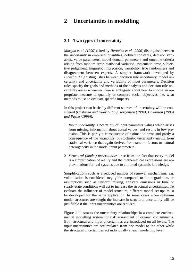
Morgan et al. (1990) (cited by Hertwich et al., 2000) distinguish betweenthe uncertainty in empirical quantities, defined constants, decision vari-ables, value parameters, model domain parameters and outcome criteriaarising from random error, statistical variation, systematic error, subjec-tive judgement, linguistic imprecision, variability, true randomness anddisagreement between experts. A simpler framework developed byFinkel (1990) distinguishes between decision rule uncertainty, model un-certainty and uncertainty and variability of input parameters. Decisionrules specify the goals and methods of the analysis and decision rule un-certainty arises whenever there is ambiguity about how to choose an ap-propriate measure to quantify or compare social objectives, i.e. whatmethods to use to evaluate specific impacts.
In this project two basically different sources of uncertainty will be con-sidered (Costanza and Sklar (1985), Jørgensen (1994), Håkanson (1995)and Payne (1999)):
1 Input uncertainty. Uncertainty of input parameter values which arisesfrom missing information about actual values, and results in low pre-cision. This is partly a consequence of estimation error and partly aconsequence of the variability, or stochastic uncertainty arising fromstatistical variance that again derives from random factors or naturalheterogeneity in the model input parameters.
2 Structural (model) uncertainties arise from the fact that every modelis a simplification of reality and the mathematical expressions are ap-proximations for real systems due to a limited systemic knowledge.
Simplifications such as a reduced number of removal mechanisms, e.g.volatilisation is considered negligible compared to bio-degradation, orassumptions such as uniform mixing, constant emissions in time orsteady-state conditions will act to increase the structural uncertainties. Toevaluate the influence of model structure, different model set-ups mustbe developed for the same application. In some cases when optimummodel structures are sought the increase in structural uncertainty will bejustifiable if the input uncertainties are reduced.
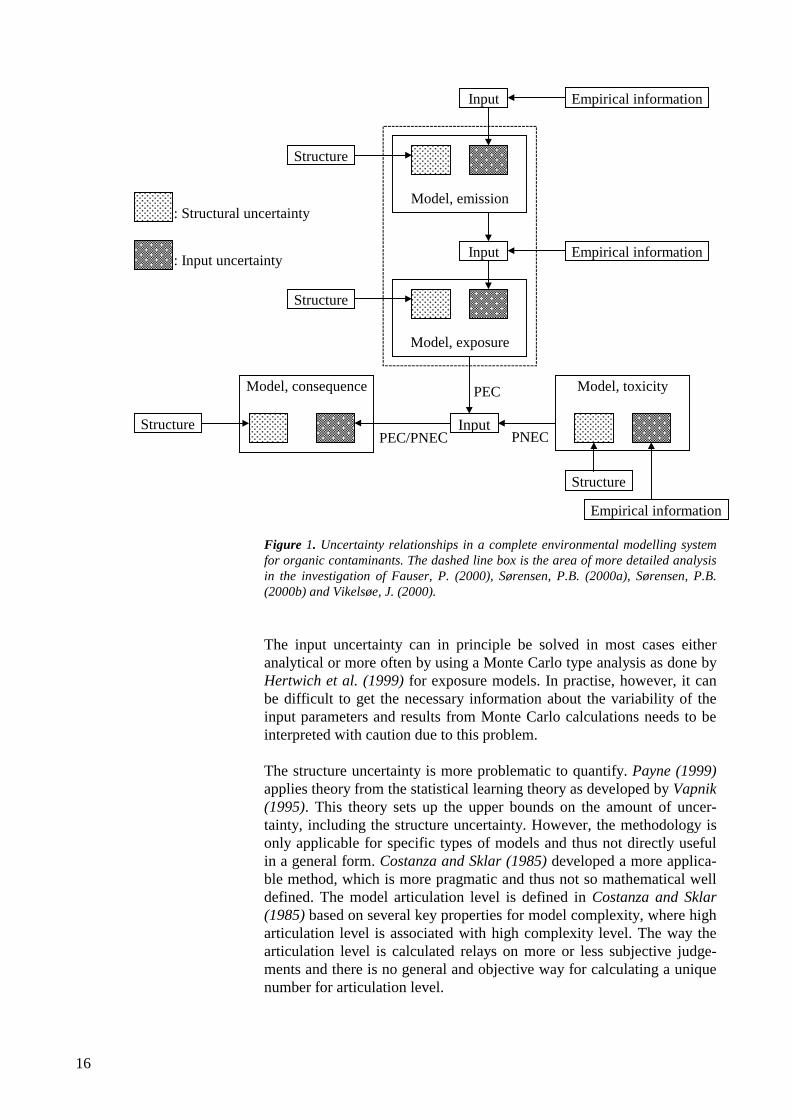
Figure 1 illustrates the uncertainty relationships in a complete environ-mental modelling system for risk assessment of organic contaminants.Both structural and input uncertainties are introduced on all levels. Theinput uncertainties are accumulated from one model to the other whilethe structural uncertainties act individually at each modelling level.
16
Figure 1. Uncertainty relationships in a complete environmental modelling systemfor organic contaminants. The dashed line box is the area of more detailed analysisin the investigation of Fauser, P. (2000), Sørensen, P.B. (2000a), Sørensen, P.B.(2000b) and Vikelsøe, J. (2000).
The input uncertainty can in principle be solved in most cases eitheranalytical or more often by using a Monte Carlo type analysis as done byHertwich et al. (1999) for exposure models. In practise, however, it canbe difficult to get the necessary information about the variability of theinput parameters and results from Monte Carlo calculations needs to beinterpreted with caution due to this problem.
The structure uncertainty is more problematic to quantify. Payne (1999)applies theory from the statistical learning theory as developed by Vapnik(1995). This theory sets up the upper bounds on the amount of uncer-tainty, including the structure uncertainty. However, the methodology isonly applicable for specific types of models and thus not directly usefulin a general form. Costanza and Sklar (1985) developed a more applica-ble method, which is more pragmatic and thus not so mathematical welldefined. The model articulation level is defined in Costanza and Sklar(1985) based on several key properties for model complexity, where higharticulation level is associated with high complexity level. The way thearticulation level is calculated relays on more or less subjective judge-ments and there is no general and objective way for calculating a uniquenumber for articulation level.
Empirical information
Model, emission
Structure
Input
Input Empirical information
Model, exposure
Structure
Model, consequence
Structure Input
Model, toxicity
Empirical information
Structure
: Structural uncertainty
: Input uncertainty
PEC
PNECPEC/PNEC

17
2.2 Uncertainty bottle neck
Even though the total uncertainty system seems complicated, there willtypically only be a few dominating sources of uncertainty. The law ofuncertainty accumulation can identify these
.....23
22
21
2total ∆+∆+∆=∆ (1)
where ∆total is the total or resulting uncertainty and ∆1 , ∆2 and ∆3 are theuncertainty contributions from different sources. ∆total can be defined fora single model or a set of sub-models, and ∆n can be uncertainties con-nected to input parameters or to individual sub-models. If all uncertaintysources are known the values can be ranked according to: ∆1 > ∆2 > ∆3
>... and equation 1 rewritten as
.... 1
2
1
3
2
1
21total +
∆∆
+
∆∆
+⋅∆=∆ (2)
This equation shows that the sources associated to the largest uncertaintyvalues will tend to dominate more than their actual values indicate. Letsconsider a numerical example where there are totally 11 sources of un-certainty having the values of:
∆1: 0,1∆2-∆11: 0,025
So in this case one source of uncertainty induces a variation of 0,1 and 10other sources induce a variation of 0,025 each. Intuitively, it should beexpected that the 10 smaller contributions of uncertainty do have a ratherlarge influence on the total uncertainty because their values are not verymuch smaller than ∆1. However, using Eq. 2 the total uncertainty is cal-culated to be ∆total=0.13, which only differs from the single uncertaintysource ∆1, by 30 %. If the uncertainty should be improved in this systemby removing one or more of the uncertainty sources two alternatives canbe considered: (1) removing of only ∆1 or (2) removing of all the uncer-tainty sources ∆2-∆11. The first alternative will reduce the uncertaintyfrom 0.13 to 0.08, while the second alternative will reduce the uncer-tainty from 0,13 to 0,1. So the elimination of only ∆1 will improve theuncertainty nearly double so much as an elimination of all the uncertaintysources ∆2-∆11. Hence, according to equation 2, ‘uncertainty bottle neck’will often exist in the model system, which will account for most of thetotal uncertainty.
The example indicates that great care must be taken where to allocate re-sources to improve the model structure. A model can be said to be dis-cordant (inharmonious) when some parts of the model operates with arelatively low uncertainty while other parts of the model includes ahigher level of uncertainty. In a discordant model minor uncertaintysources have been improved at the expense of major uncertainty sources.However, if all information needed for an existing discordant model isavailable then the model can be used without consideration as a ‘best
18
obtainable knowledge approach’. The problems arise if such a model isused to identify data necessary for the decision making, because re-sources are wasted on collecting superfluous information. Furthermore, adiscordant model can easily produce conclusions of false realism whendetailed parameter studies of low uncertainty sources are consideredwhen the emphasis should be on other parts of the model.
2.3 Ranking of completity level
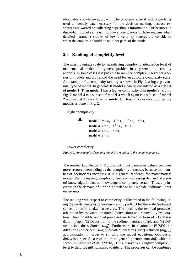
The missing unique scale for quantifying complexity articulation level ofmathematical models is a general problem in a systematic uncertaintyanalysis. In some cases it is possible to rank the complexity level for a se-ries of models and thus avoid the need for an absolute complexity scale.An example of a complexity ranking is shown in Fig. 2 using a polyno-mial type of model. In general: If model 2 can be considered as a sub setof model 1. Then model 1 has a higher complexity than model 2. E.g. inFig. 2 model 4 is a sub set of model 3 which again is a sub set of model2 and model 2 is a sub set of model 1. Thus, it is possible to order themodels as done in Fig. 2.
o
o
o
o
a=y:
a+xa=y:
a+xa+xa=y:
a+xa+xa+xa=y:
4model
3model
2model
1model
1
12
2
12
23
3
Figure 2. An example of ranking models in relation to the complexity level.
The needed knowledge in Fig 2 about input parameter values becomesmore resource demanding as the complexity increases because the num-ber of coefficients increases. It is a general tendency for mathematicalmodels that increasing complexity yields an increasing demand of a pri-ori knowledge. In fact no knowledge is completely certain. Thus, any in-crease in the demand of a priori knowledge will include additional inputuncertainty.
The ranking with respect to complexity is illustrated in the following us-ing the model analysis in Sørensen et al., (2001a) for the water/sedimentconcentration in a lake/marine area. The focus is the removal processesother than hydrodynamic removal (convection) and removal by evapora-tion. Three possible removal processes are leaved in form of: (1) degra-dation (degr), (2) Deposition to the sediment surface (dep), and (3) Dif-fusion into the sediment (diff). Furthermore in relation to EUSES thediffusion is described using a so-called thin film (layer) diffusion (difffilm)approximation in order to simplify the model equations. Obviously,difffilm is a special case of the more general phenomenon diff, which isshown in Sørensen et al., (2001a). Thus, it involves a higher complexitylevel to describe diff compared to difffilm. The processes can be combined
Higher complexity
Lower complexity
19
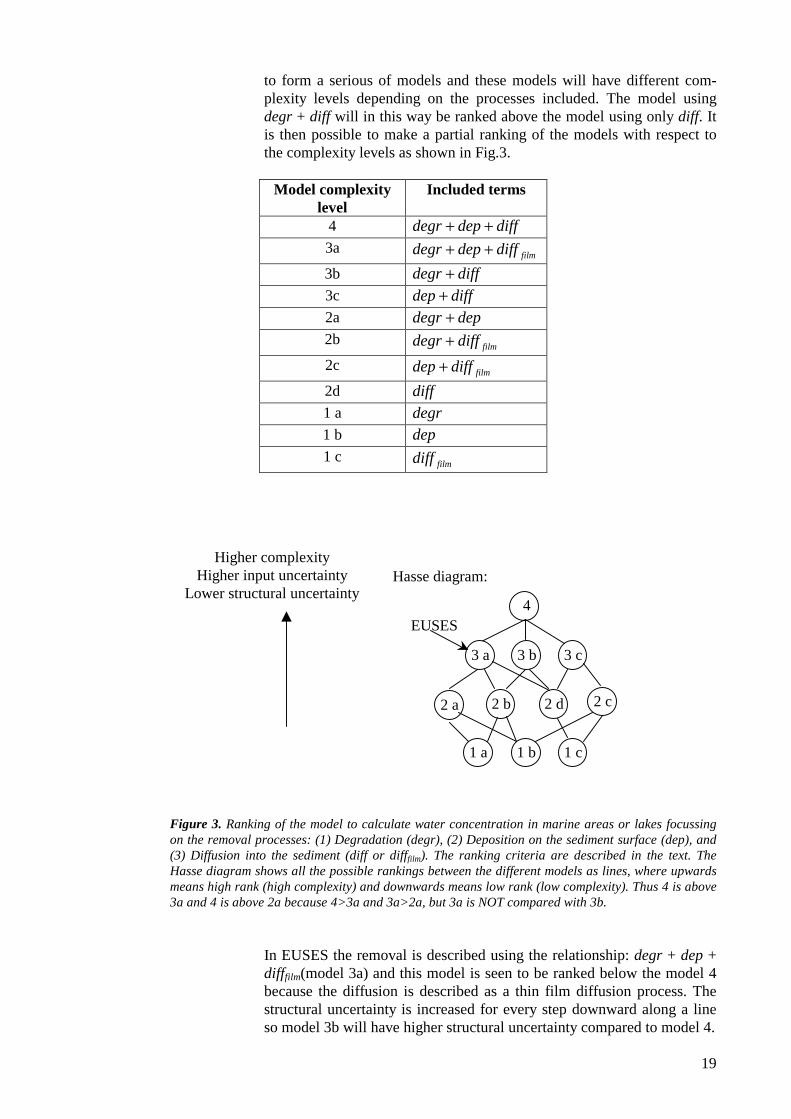
to form a serious of models and these models will have different com-plexity levels depending on the processes included. The model usingdegr + diff will in this way be ranked above the model using only diff. Itis then possible to make a partial ranking of the models with respect tothe complexity levels as shown in Fig.3.
Model complexitylevel
Included terms
4 diffdepdegr ++3a
filmdiffdepdegr ++3b diffdegr +3c diffdep +2a depdegr +2b
filmdiffdegr +2c
filmdiffdep +2d diff1 a degr1 b dep1 c
filmdiff
Figure 3. Ranking of the model to calculate water concentration in marine areas or lakes focussingon the removal processes: (1) Degradation (degr), (2) Deposition on the sediment surface (dep), and(3) Diffusion into the sediment (diff or difffilm). The ranking criteria are described in the text. TheHasse diagram shows all the possible rankings between the different models as lines, where upwardsmeans high rank (high complexity) and downwards means low rank (low complexity). Thus 4 is above3a and 4 is above 2a because 4>3a and 3a>2a, but 3a is NOT compared with 3b.
In EUSES the removal is described using the relationship: degr + dep +difffilm(model 3a) and this model is seen to be ranked below the model 4because the diffusion is described as a thin film diffusion process. Thestructural uncertainty is increased for every step downward along a lineso model 3b will have higher structural uncertainty compared to model 4.
4
3 a 3 b 3 c
2 a 2 d2 b
1 a 1 b 1 c
Higher complexityHigher input uncertainty
Lower structural uncertainty
2 c
EUSES
Hasse diagram:

20
On the other hand step downward will in general yield lower input-uncertainty and a model, which is less, complicated to handle mathe-matically. This is the argument for selecting model 3b instead of model4.
The conclusion in Sørensen et al., (2001a) is that the diffusion process isnot well described by the thin layer diffusion approximation. It is alsoshown that often the removal by diffusion (diff) can be neglected com-pared to the removal by deposition (dep). Thus, a step downward in theHasse diagram in Fig. 3 from 3a to 2a is beneficial because it will reducethe complexity and thereby reduce both the input uncertainty and the re-sources demand for the model to be used without increasing the struc-tural uncertainty remarkable.

21
3 The concept of obtimal complexity
Some complexity is needed for any prediction and an increase in com-plexity enhance the opportunities for a closer and thus more certain de-scription of reality (decreased structure-uncertainty). So there seems tobe a dilemma between the demand of low input uncertainty (low com-plicity) and a low structural uncertainty (high complexity). The optimalmodel structure based on the actual a priori knowledge is a compromisebetween these two sources of uncertainty. The model structure can beoptimised through a mutual evaluation of the input and structural uncer-tainties. The problem is to quantify the uncertainties, where especiallythe structural uncertainty can form a problem as discussed above. How-ever, by using the concept of relative complexity it may under some cir-cumstances be possible to identify the optimal model complexity as ex-emplified below.
The principle is illustrated in the following, where three different modelsare mutually ranked with respect to complexity as illustrated above. Theexample of uncertainty analysis is based on the work of Vikelsøe et al.,(2001) and the details is shown in Appendix A. The problem in the ex-ample is to calculate the dissolved water concentration at a specific depthbelow the sediment surface. The depth is chosen to be 1 cm and onlysteady state conditions are considered. Three different models havingthree different complexity levels is formulated for the same problem anduncertainty is calculated for each model. However, as pointed out earlierthe structural uncertainty is difficult to quantify so the relative structuraluncertainty (relative to the most complex model) is calculated instead.The calculation of the relative structural uncertainty is described in theAppendix and illustrated in Fig. 3A in appendix.
The results of the analysis is shown in Fig. 4, where the two types of un-certainty is shown for the three models, which are ranked in relation tothe level of complexity. The simplest model (model 3) does not includeany processes and thus simply assumes the water concentration in thesediment to equalise the water concentration in the water column. Theinput uncertainty is therefore equal zero under these circumstances. Thebest model is seen to be model 2, which includes deposition and degra-dation but neglects diffusion.

22
Figure 4. This is a Illustration of complexity ranking, where a series of models are identified assubsets of each other. It is not possible to quantify the absolute structural uncertainty for model 1.But, it is possible to determinate the increase in structural uncertainty (additional structural un-certainty) between the different models as illustrated by the dashed line. For the optimal model thesum of the additional structural uncertainty and the input uncertainty is minimal (model 2 in thiscase).
However, in praxis the principle is difficult to use in real uncertainty cal-culations due to difficulties in quantifying the complexity. The problemof quantifying complexity is solved in the example above by ranking themodel complexity as described in Fig. 4, where different number of termsare added in the governing differential equations. In this way it is onlypossible to place the different models on the complexity level axis in Fig.5 relative to each other. However, it will still be possible to keep the con-cept of a continuously scale for complexity in order to develop a methodwhich can help to select the “best” model from possible alternativeshaving the lowest total uncertainty.
The structure uncertainty is difficult to quantify completely, but it is notnecessary to make a complete quantification in order to find the optimalmodel complexity. In the example above only the differences in structureuncertainty values are calculated as the value difference between themost complex model (Model 1, having the lowest structural uncertainty)and the other models (Models 2 and 3). In this way the quantified part ofthe structure uncertainty for the Models 2 and 3 is the addition in struc-ture uncertainty when either Model 2 or 3 replaces Model 1. By using
Complexity
Uncertainty: (absolute structural) +(absolute input)
Model 3:
dz
dCS ⋅=0
: Structural uncertainty : Input uncertainty
Signature:
Additional structural uncertainty:Model 1 – Model 2=0.02
Additional structural uncertainty:Model 1 – Model 3=0.24
Uncertainty: (Additional structural) + (absolute input)
Model 2:
CR
k
dz
dCS ⋅−⋅= 10
Model 1:
CR
k
dz
dCS
dz
Cd
R
D ⋅−⋅−⋅= 12
2
0
Absolute structural uncertaintyfor Model 1
0.13
0.07

23
this principle, the total uncertainty, as illustrated in Fig. 5, will be re-placed by the fraction of the total uncertainty formed by adding the inputuncertainty to the differences in structural uncertainty between Model 1and Model 2, and between Model 1 and Model 3, respectively. The re-duced total uncertainty will become equal to the input uncertainty forModel 1 simply because the reduced structure uncertainty is zero in thiscase.
Payne (1999) discusses the relationship between uncertainty and com-plexity level in general terms as illustrated in the example above. Theproblem is illustrated graphically in Fig. 5.
Figure 5. The relationship between the structural uncertainty and the input uncertainty. Vapnik(1995) shows similar relationships.
Fig. 5 is a principal figure, which summarises the conclusion, in thischapter. The input uncertainty is claimed to increase and the structureuncertainty is claimed to decrease as the model complexity is increased.Obviously, the resulting total uncertainty will tend to have a minimumvalue at the optimal complexity level yielding the lowest total uncer-tainty. This figure represents a systematic paradigm for model evaluationand will form the basis in the tiered approach for uncertainty analysis in acoming chapter.
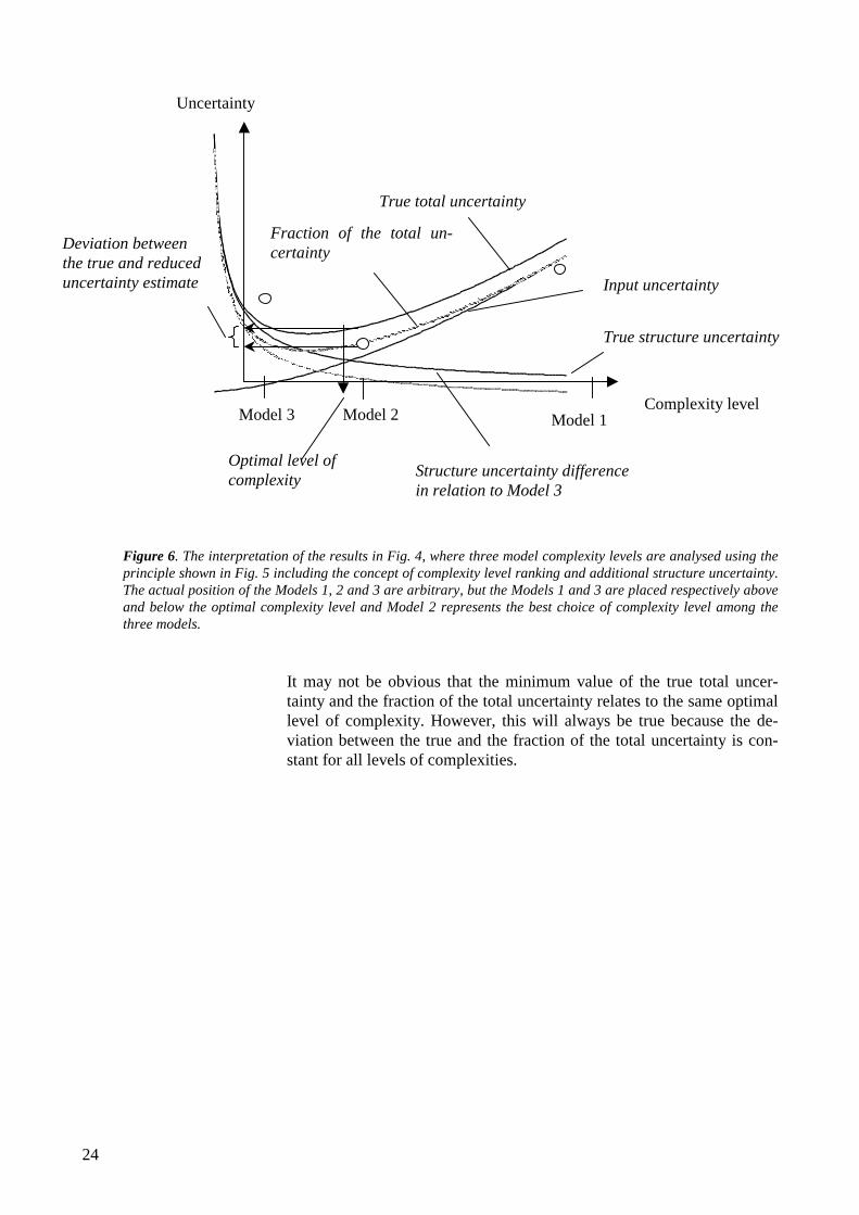
The use of complexity rank and reduced structure uncertainty is illus-trated in Fig. 6, where the three Models 1, 2, and 3 are shown for illus-tration. The actual placements of the three models on the complexityscale are unknown. However, due to the complexity level rank as Model1 > Model 2 > Model 3 it must be true that the position of Model 3 is at alower complexity level than the optimal level and Model 1 needs to beplaced at a higher complexity level than the optimal level. This is truebecause the total reduced uncertainty for Model 2 is lower than for thetwo other models.
Complexity level
Uncertainty
Structure uncertainty
Input uncertainty
Total uncertainty
Optimal complexity level
Minimal uncertainty
24
Figure 6. The interpretation of the results in Fig. 4, where three model complexity levels are analysed using theprinciple shown in Fig. 5 including the concept of complexity level ranking and additional structure uncertainty.The actual position of the Models 1, 2 and 3 are arbitrary, but the Models 1 and 3 are placed respectively aboveand below the optimal complexity level and Model 2 represents the best choice of complexity level among thethree models.
It may not be obvious that the minimum value of the true total uncer-tainty and the fraction of the total uncertainty relates to the same optimallevel of complexity. However, this will always be true because the de-viation between the true and the fraction of the total uncertainty is con-stant for all levels of complexities.
True total uncertainty
Fraction of the total un-certainty
Input uncertainty
True structure uncertainty
Structure uncertainty differencein relation to Model 3
Complexity level
Uncertainty
Model 3 Model 2 Model 1
Deviation betweenthe true and reduceduncertainty estimate
Optimal level ofcomplexity

25
4 The relation ship between information’slevel of model result and uncertainty
The model structure uncertainty depends on the choice of the outcome,i.e. what question needs to be answered and thus the amount of informa-tion (knowledge) that is required from the model. In the shown examplethe question was about the steady-state concentration at a depth of 1 cmin the sediment and it was not the most complex model that had thesmallest total uncertainty. If the demand of information increases in thequestion to comprise the concentration change in time in the depth of 1cm, the diffusion will play an important role and model 1 will probablybe needed. In the immediate upstart of the system, i.e. for t = 0, the con-centration gradient will be large at the sediment surface and the substrateflux to the sediment will be governed by diffusion and not by sedimenta-tion. After a number of days the amount of substrate originating fromsedimentation will dominate. In Sørensen et al. (2001a) the change inprocess kinetics is described.
The input uncertainty curve is identical to the one with a lower informa-tion level, whereas the uncertainty curve for the model structure has in-creased caused by the need of more complex structures to answer for thedesire of more detailed information (higher information level). This isvery importance to realise for a decision-maker that asks an ‘expert’about a prediction to support a decision. If the question is formulated tothe expert at a higher information level than strictly necessary for the de-cision then a lot of resources can easily be wasted. This problem is illus-trated in Fig. 7 and has been formulated in the statistical learning theoryfor problem solution using a restricted amount of information as: Whensolving a given problem, try to avoid solving a more general problem asan intermediate step (Vapnik, 1995).

26
Informationsværdi
Structureuncertainty
InputuncertaintyTotal
uncertainty
Uncertainty
Complexitylevel
Structureuncertainty
Inputuncertainty
Total uncertaintyUncertainty
Complexitylevel
Information level
Figure 7. Influence of level of information on the optimum model structure com-plexity. Similar relationships are discussed by Vapnik, (1995).
When mathematical models are needed to support decision-making it iscritical to be aware of this close relationship between the needed infor-mation level of the result and the uncertainty of the prediction. A dialogis important between the model designer/developer and the model user.Unfortunately, in the process of model development the model user (de-cision maker) sets up the goal (question to be answered at a given infor-mation level) and then subsequently the model designer tries to fulfil thegoals as good as possible without any dialog with the model user. It caneasily happen that the model results turns out to be very uncertain, but aslight reduction in the information level of the results (less ambitiousmodel answer) may improve the result certainty dramatically.

27
5 Tiered approach for uncertainty analy-sis
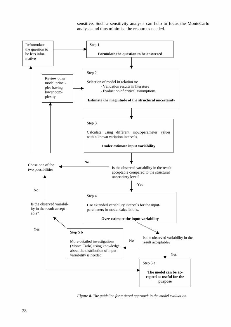
A close evaluation of model uncertainty is in general a rather resourcedemanding task and in reality the user of a model can easily be broughtinto a situation where a model have to be used without the possibility forsuch an evaluation. A possible way to deal with this situation can be touse a kind of tiered approach where more easy screening methods canhelp to identify model uncertainty in relation to a specific problem. Aguideline for such an approach is shown in Figure 8 and will be ex-plained in the following.
Step 1. The formulation of the problem to be solved in terms of a ques-tion to answer is crucial for the following choice and evaluation of themodel. It is therefore important to make a precise formulation of thequestion.
Step 2. The model is selected based on expert judgement, which again isbased on reported validation results and an evaluation of critical assump-tions. The magnitude of the structural uncertainty needs to be quantifiedso much as possible. The structural uncertainty is difficult to quantifyhowever, some kind of judgement is necessary and in most cases possi-ble.
Step 3. As a first approach a few model calculations are done using rela-tively few different combination of realistic input parameters. There willoften exist an a priori knowledge, about which of the input parametersthat are the most important for the model and about an interval of varia-tion, which is smaller than the true variability. If the variation of inputparameter values in this analysis yields results of unacceptable high un-certainty then is possible to reject the model as a candidate for valid cal-culations.
Step 4. If the model uncertainty was acceptable in step 3, the next stepwill be to over estimate the input-uncertainty, where unrealistic varia-tions is applied to the input. More effort is needed in this step comparedto step 3 but in many cases it will be a rather easy task to set up an overestimation of the variability intervals. If the input-uncertainty is accept-able then the model prediction will be valid otherwise more detailed andthus also much more resource demanding uncertainty analysis needs tobe applied.
Step 5 a. The model is acceptable and can be used to answer the ques-tion. There may exist a more complex model which can make an answerat a higher information level than the actual question.
Step 5 b. A detailed uncertainty analysis is made for input-uncertainty.The information needed is knowledge about the distribution function forinput-parameter variability, which can be used in a Monte Carlo simula-tion. In some cases a sensitivity analysis can be used before the Monte-Carlo analysis to identify the parameters for which the model is most
28
sensitive. Such a sensitivity analysis can help to focus the MonteCarloanalysis and thus minimise the resources needed.
Figure 8. The guideline for a tiered approach in the model evaluation.
Step 1
Formulate the question to be answered
Step 3
Calculate using different input-parameter valueswithin known variation intervals.
Under estimate input variability
Is the observed variability in the resultacceptable compared to the structuraluncertainty level?
No
Review othermodel princi-ples havinglower com-plexity
Yes
Step 4
Use extended variability intervals for the input-parameters in model calculations.
Over estimate the input variability
Is the observed variability in theresult acceptable?No
Yes
Step 5 b
More detailed investigations(Monte Carlo) using knowledgeabout the distribution of input-variability is needed.
Step 5 a
The model can be ac-cepted as useful for the
purpose
Step 2
Selection of model in relation to:- Validation results in literature- Evaluation of critical assumptions
Estimate the magnitude of the structural uncertainty
Is the observed variabil-ity in the result accept-able?
No
Yes
Reformulatethe question tobe less infor-mative
Chose one of thetwo possibilities

29
6 Perspective in relation to a specific xe-nobiotic fate analysis
This report is a part of a project where models are evaluated for four spe-cific systems, each one being a part of an overall system describing theflow of xenobiotics in Roskilde municipality and catchment area (seefigure 7). The models is discussed in relation to their harmony (Samelevel of uncertainty in all parts of the model) and their Input/structureuncertaintyes (The input uncertainty is related to the structure uncer-tainty). The results is summerised in Carlsen et al. (2001).
Survey Sources and emissions of the xenobiotics in question.Model 1 Fate of substances in Roskilde WWTP (Fauser et al. 2001).Model 2 Fate of substances in Roskilde Fjord (water and sediment)
(Vikelsøe et al. 2001 and Sørensen et al. 2001).Model 3 Fate of substances in sewage sludge amended soil.
Top SoilLeaching
Figure 7. Schematic overview of modelling system.
These four models can be used separately; however, the combined ap-proach permits an integrated uncertainty analysis of the total emis-sion/fate modelling system. The emission survey gives input concentra-tions to the WWTP, the effluent water and digested sludge from theWWTP provide input data to Roskilde inlet and the field plough layer re-spectively.
The product will be risk assessment models designed to estimate Pre-dicted Environmental Concentrations (PEC) of LAS, 6 different phtha-lates, nonylphenol and nonylphenol diethoxylate in the water and soilcompartments. Experimental data, generated from laboratory experi-
Surface runoff
Industryand service
Sewer
Emission survey
WWTP modelHouseholds
Soil
Inlet model
Sewage
Sludge
Treated water
P
S
Sediment

30
ments and in-situ monitoring studies provide data for calibration andverification of the models. They act as a tool to estimate the PredictedNo-effect Concentrations (PNEC) and in this way help to decide whetheror not a substance presents a risk to the environment.

31
7 References
Carlsen,L., Sørensen, P.B., Vikelsøe,J., Fauser,P. and Thomsen, M.(2001): On the fate of Xenobiotics. The Roskilde region as case story,NERI report (in press)
Costanza, R. and F. H. Sklar, (1985): Ariculation, Accuracy and Effec-tiveness of Mathematical Models: A Review of Freshwater Wetland Ap-plications, Ecological Modelling, 27, pp. 45-68.
"EUSES, the European Union System for the Evaluation of Substances"EUSES 1.00 User Manual. February 1997, TSA Group Delft by, Euro-pean Commission - JRC, Existing Chemicals T. P. 280, 1-21020 Ispra(VA), Italy
Fauser,P., Sørensen,P.B., Vikelsøe,J., and L. Carlsen (2001): Phthalates,Nonylphenols and LAS in Roskilde Wastewater Treatment Plant - FateModelling Based on Measured Concentrations in Wastewater andSludge. NERI report (in press)
Hertwich. E. G., T. E. McKone and W. S. Pease (1999):Parameter Un-certainty and Variability In Evaluative Fate and Exposure Models, RiskAnalysis, Vol. 19, No. 6.
Hertwich E. G., T. E. Mckone and W. S. Pease (2000): A Systematic Un-certainty Analysis of an Evaluative Fate and Exposure Model, RiskAnalysis, Vol. 20, No. 4.
Håkanson, L., (1995): Optimal Size of Predictive Models, EcologicalModelling, 78, pp. 195-204.
Jørgensen, S. E., (1994): Fundamentals of Ecological Modelling (2nd
Edition), Elsevier Science B. V.
Kann, A. and J. P. Weyant, (2000): Approaches for performing uncer-tainty analysis in larger-scale energy/economic policy models, Environ-mental Modelling and Assessment, 5, pp. 29-46.
Payne, K., (1999): The VC dimension and ecological modelling, Eco-logical Modelling, 118, pp. 249-259.
Sørensen, P.B., P. Fauser, L. Carlsen and J. Vikelsøe, (2001a): Theo-retical evaluation of the sediment/water exchange description in genericcompartment models (SimpleBox). NERI report (in press)
Sørensen,P. B., L. Carlsen, J. Vikelsøe and A. G. Rasmussen (2001b):Modelling analysis of sewage sludge amended soil. NERI report (inpress)
Vapnik, V. N., (1995): The Nature of Statistical Learning Theory,Springer-Verlag New York, Inc.

32
Vikelsøe, J., P. Fauser, P. B. Sørensen, L. Carlsen (2001): Phthalates andNonylphenols in Roskilde Fjord - A Field Study and MathematicalModelling of Transport and Fate in Water and Sediment. NERI report (inpress)

33
Appendix A: Example of quantifying uncer-tainty
As an illustrative example, the optimum model structure is sought for ina scenario involving transport and degradation of a hydrophobic, slowlydegradable substrate in the sediment compartment in a water-sedimentsystem corresponding to the Fjord model described in Vikelsøe et al.(2000).
Three different models having three different complexity levels will beformulated for the same problem. So the analysis will be based on rankedcomplexity as illustrated in Fig. 4. This example will show how the in-put- and the structural uncertainty, respectively, interacts in relation tothe total model uncertainty.
The following assumption are made
• Steady-state. i.e. 0 t
C =∂∂
. A detailed analysis of this simplification
can be found in Sørensen et al. (2000).
• 1st order degradation of dissolved substrate (k1).
• Equilibrium between adsorbed and dissolved substrate, describedthrough the equilibrium partition coefficient Kd.
• Constant pore water volume, θ, and thus concentration of particulatematter, X, in sediment. The retention factor, R = θ + X ⋅ Kd, willtherefore also be constant throughout the sediment profile.
• Vertical molecular diffusive flow (D).
• Constant sedimentation (solids deposition) rate at the sediment sur-face (S).
The structural, input and total uncertainties related to the steady-statedissolved concentration at a depth of 1 cm will be calculated for the threemodels.
Each input parameter is associated with an (input) uncertainty expressedas a standard deviation
Adsorption: R = 10600 ± 1000Degradation: k1 = 2 ⋅ 10-5 ± 5 ⋅ 10-6 sec-1
Diffusion: D = 10-10 ± 5 ⋅ 10-11 m2 ⋅ sec-1
Sedimentation:S = 2.5 ± 0.5 mm ⋅ year-1
The dissolved pore water concentration in the surface layer is C0 = 1 µg ⋅liter-1.

34
Model 1: The more complex model. So, the relative structural uncer-tainty is calculated based on this model (like model 1 in Fig.4). The model comprises adsorption (R), degradation (k1),diffusion (D) and sedimentation (S).
The concentration profile is expressed through the linear, one dimen-sional and homogeneous 2nd order equation
C R
k -
dz
dC S -
dz
Cd
R
D 0
t
C 12
2
⋅⋅⋅==∂∂
(3)
the solution being (Vikelsøe et al., 2000)
z D
k +
2 D
R S -
2 D
R S
01 model
12
e C = z)(C⋅
⋅⋅
⋅⋅
⋅ (4)
The mean concentration, Cmean,model 1, which is equal to the exact concen-tration, Cexact, is found from n = 2000 random Monte Carlo type selec-tions of the normally distributed input values and insertion in Equation 4.
liter
g 0.7667 C
n
1 C C
n
1 i1 modeli,exact1 modelmean,
µ=⋅== ∑=
Model 2: Includes adsorption (R), degradation (k1) and sedimentation(S). The diffusion process is omitted in relation to Model 1.
The concentration profile is now defined by
C R
k -
dz
dC S - 0
t
C 1 ⋅⋅==∂∂
(5)
with the solution
R S
z k -
02 model
1
e C )z(C ⋅⋅
⋅= (6)
and a mean concentration
liter
g 0.7810 C
n
1 C
n
1 i2 modeli,2 modelmean,
µ=⋅= ∑=
Model 3: The most simple model. Only adsorption (R) and sedimenta-tion (S) are considered and the steady-state concentration pro-file will therefore be constant and equal to C0.
liter
g 1 C 3 modelmean,
µ=
35
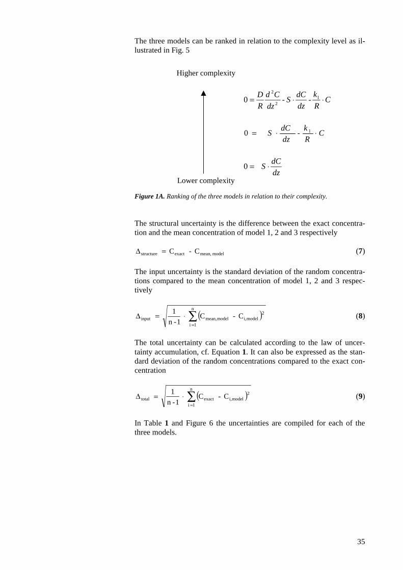
The three models can be ranked in relation to the complexity level as il-lustrated in Fig. 5
Figure 1A. Ranking of the three models in relation to their complexity.
The structural uncertainty is the difference between the exact concentra-tion and the mean concentration of model 1, 2 and 3 respectively
model mean,exactstructure C - C =∆ (7)
The input uncertainty is the standard deviation of the random concentra-tions compared to the mean concentration of model 1, 2 and 3 respec-tively
( )∑=
⋅=∆n
1 i
2modeli,modelmean,input C - C
1 -n
1 (8)
The total uncertainty can be calculated according to the law of uncer-tainty accumulation, cf. Equation 1. It can also be expressed as the stan-dard deviation of the random concentrations compared to the exact con-centration
( )∑=
⋅=∆n
1 i
2modeli,exacttotal C - C
1 -n
1 (9)
In Table 1 and Figure 6 the uncertainties are compiled for each of thethree models.
CR
k
dz
dCS
dz
Cd
R
D ⋅⋅= 12
2
--0
CR
k
dz
dCS ⋅⋅= 1-0
dz
dCS ⋅=0
Higher complexity
Lower complexity

36
Table 1 Structural, input and total uncertainties for 3 different models ofvarying complexities. The models calculate the steady-state concentra-tion at a depth of 1 cm in the sediment. Units in µg ⋅ liter-1.
Model 1 Model 2 Model 3Structural uncertainty(Equation 7)
0 0,02 0,24
Input uncertainty(Equation 8)
0,13 0,07 0
Total uncertainty(Equation 9)
0,13 0,07 0,24
0
0 ,0 5
0 ,1
0 ,1 5
0 ,2
0 ,2 5
M od el 3 M od el 2 M od el 1L evel of com p lex i ty
Unc
erta
inty
[µ
g *
liter
-1]
S tru ctu re
In p u t
T ota l
Figure 2A. Structural, input and total uncertainties for 3 different models of varyingcomplexities. The models calculate the steady-state concentration at a depth of 1 cmin the sediment.
The model complexity decreases from model 1 through 3 and accord-ingly the structural uncertainties increase from zero to approximately0.238 for model 3. As previously noted model 1 is considered to producethe exact result but in reality this is not true and the structural uncertaintyassociated with model 1 will be different from zero, but still smaller thanmodel 2 and 3. The more complex model 1 requires more input data andtherefore the input uncertainty is larger than for model 2 and 3.
The differences in structural and input uncertainties between model 1 and2 arise from the influence of diffusion. At a depth of 1 cm the substratemass arising from molecular diffusion is larger than deeper down in thesediment which implies that the differences in structural and input un-certainties between model 1 and 2 are larger closer to the sediment sur-face, cf. Equations 7 and 8. At larger depths, below approximately 0.5 m,the deviation between the output from model 1 and 2 is negligible andaccordingly the structural, input and total uncertainties are identical.However, model 1 still requires more information about the input pa-rameters, i.e. the diffusion coefficient.
37
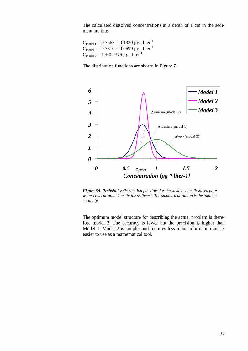
The calculated dissolved concentrations at a depth of 1 cm in the sedi-ment are thus
Cmodel 1 = 0.7667 ± 0.1330 µg ⋅ liter-1
Cmodel 2 = 0.7810 ± 0.0699 µg ⋅ liter-1
Cmodel 3 = 1 ± 0.2376 µg ⋅ liter-1
The distribution functions are shown in Figure 7.
0
1
2
3
4
5
6
0 0,5 1 1,5 2Concentration [µg * liter-1]
Model 1
Model 2
Model 3∆structure(model 2)
∆ structure(model 1)
∆ input(model 3)
Cexact
Figure 3A. Probability distribution functions for the steady-state dissolved porewater concentration 1 cm in the sediment. The standard deviation is the total un-certainty.
The optimum model structure for describing the actual problem is there-fore model 2. The accuracy is lower but the precision is higher thanModel 1. Model 2 is simpler and requires less input information and iseasier to use as a mathematical tool.

38
National Environmental Research Institute
The National Environmental Research Institute, NERI, is a research institute of the Ministry of Environment and En-ergy. In Danish, NERI is called Danmarks Miljøundersøgelser (DMU).NERI's tasks are primarily to conduct research, collect data, and give advice on problems related to the environment andnature.
Addresses: URL: http://www.dmu.dk
National Environmental Research InstituteFrederiksborgvej 399PO Box 358DK-4000 RoskildeDenmarkTel: +45 46 30 12 00Fax: +45 46 30 11 14
ManagementPersonnel and Economy SecretariatResearch and Development SectionDepartment of Atmospheric EnvironmentDepartment of Environmental ChemistryDepartment of Policy AnalysisDepartment of Marine EcologyDepartment of Microbial Ecology and BiotechnologyDepartment of Arctic Environment
National Environmental Research InstituteVejlsøvej 25PO Box 314DK-8600 SilkeborgDenmarkTel: +45 89 20 14 00Fax: +45 89 20 14 14
Environmental Monitoring Co-ordination SectionDepartment of Lake and Estuarine EcologyDepartment of Terrestrial EcologyDepartment of Streams and Riparian areas
National Environmental Research InstituteGrenåvej 12-14, KaløDK-8410 RøndeDenmarkTel: +45 89 20 17 00Fax: +45 89 20 15 15
Department of Landscape EcologyDepartment of Coastal Zone Ecology
Publications:NERI publishes professional reports, technical instructions, and the annual report. A R&D projects' catalogue is avail-able in an electronic version on the World Wide Web.Included in the annual report is a list of the publications from the current year.

39
Faglige rapporter fra DMU/NERI Technical Reports
2000Nr. 310: Hovedtræk af Danmarks Miljøforskning 1999. Nøgleindtryk fra Danmarks Miljøundersøgelsers jubilæumskon-
ference Dansk Miljøforskning. Af Secher, K. & Bjørnsen, P.K. (i trykken)Nr. 311: Miljø- og naturmæssige konsekvenser af en ændret svineproduktion. Af Andersen, J.M., Asman, W.A.H., Hald,
A.B., Münier, B. & Bruun, H.G. (i trykken)Nr. 312: Effekt af døgnregulering af jagt på gæs. Af Madsen, J., Jørgensen, H.E. & Hansen, F. 64 s., 80,00 kr.Nr. 313: Tungmetalnedfald i Danmark 1998. Af Hovmand, M. & Kemp, K. (i trykken)Nr. 314: Future Air Quality in Danish Cities. Impact Air Quality in Danish Cities. Impact Study of the New EU Vehicle
Emission Standards. By Jensen, S.S. et al. (in press)Nr. 315: Ecological Effects of Allelopathic Plants – a Review. By Kruse, M., Strandberg, M. & Strandberg, B. 64 pp.,
75,00 DKK.Nr. 316: Overvågning af trafikkens bidrag til lokal luftforurening (TOV). Målinger og analyser udført af DMU. Af Her-
tel, O., Berkowicz, R., Palmgren, F., Kemp, K. & Egeløv, A. (i trykken)Nr. 317: Overvågning af bæver Castor fiber efter reintroduktion på Klosterheden Statsskovdistrikt 1999. Red. Berthel-
sen, J.P. (i trykken)Nr. 318: Order Theoretical Tools in Environmental Sciences. Proceedings of the Second Workshop October 21st, 1999
in Roskilde, Denmark. By Sørensen, P.B. et al. ( in press)Nr. 319: Forbrug af økologiske fødevarer. Del 2: Modellering af efterspørgsel. Af Wier, M. & Smed, S. (i trykken)Nr. 320: Transportvaner og kollektiv trafikforsyning. ALTRANS. Af Christensen, L. 154 s., 110,00 kr.Nr. 321: The DMU-ATMI THOR Air Pollution Forecast System. System Description. By Brandt, J., Christensen, J.H.,
Frohn, L.M., Berkowicz, R., Kemp, K. & Palmgren, F. 60 pp., 80,00 DKK.Nr. 322: Bevaringsstatus for naturtyper og arter omfattet af EF-habitatdirektivet. Af Pihl, S., Søgaard, B., Ejrnæs, R.,
Aude, E., Nielsen, K.E., Dahl, K. & Laursen, J.S. 219 s., 120,00 kr.Nr. 323: Tests af metoder til marine vegetationsundersøgelser. Af Krause-Jensen, D., Laursen, J.S., Middelboe, A.L.,
Dahl, K., Hansen, J. Larsen, S.E. 120 s., 140,00 kr.Nr. 324: Vingeindsamling fra jagtsæsonen 1999/2000 i Danmark. Wing Survey from the Huntig Season 1999/2000 in
Denmark. Af Clausager, I. 50 s., 45,00 kr.Nr. 325: Safety-Factors in Pesticide Risk Assessment. Differences in Species Sensitivity and Acute-Chronic Relations.
By Elmegaard, N. & Jagers op Akkerhuis, G.A.J.M. 57 pp., 50,00 DKK.Nr. 326: Integrering af landbrugsdata og pesticidmiljømodeller. Integrerede MiljøinformationsSystemer (IMIS). Af
Schou, J.S., Andersen, J.M. & Sørensen, P.B. 61 s., 75,00 kr.Nr. 327: Konsekvenser af ny beregningsmetode for skorstenshøjder ved lugtemission. Af Løfstrøm, L. (Findes kun i
elektronisk udgave)Nr. 328: Control of Pesticides 1999. Chemical Substances and Chemical Preparations. By Krongaard, T., Petersen, K.K.
& Christoffersen, C. 28 pp., 50,00 DKK.Nr. 329: Interkalibrering af metode til undersøgelser af bundvegetation i marine områder. Krause-Jensen, D., Laursen,
J.S. & Larsen, S.E. (i trykken)Nr. 330: Digitale kort og administrative registre. Integration mellem administrative registre og miljø-/naturdata. Energi-
og Miljøministeriets Areal Informations System. Af Hansen, H.S. & Skov-Petersen, H. (i trykken)Nr. 331: Tungmetalnedfald i Danmark 1999. Af Hovmand, M.F. Kemp, K. (i trykken)Nr. 332: Atmosfærisk deposition 1999. NOVA 2003. Af Ellermann, T., Hertel, O. &Skjødt, C.A. (i trykken)Nr. 333: Marine områder – Status over miljøtilstanden i 1999. NOVA 2003. Hansen, J.L.S. et al. (i trykken)Nr. 334: Landovervågningsoplande 1999. NOVA 2003. Af Grant, R. et al. (i trykken)Nr. 335: Søer 1999. NOVA 2003. Af Jensen, J.P. et al. (i trykken)Nr. 336: Vandløb og kilder 1999. NOVA 2003. Af Bøgestrand J. (red.) (i trykken)Nr. 337: Vandmiljø 2000. Tilstand og udvikling. Faglig sammenfatning. Af Svendsen, L.M. et al.(i trykken)Nr. 338: NEXT I 1998-2003 Halogenerede Hydrocarboner. Samlet rapport over 3 præstationsprøvnings-runder . Af
Nyeland, B. & Kvamm, B.L.Nr. 339: Phthalates and Nonylphenols in Roskilde Fjord. A Field Study and Mathematical Modelling of Transport and
Fate in Water and Sediment. The Aquatic Environment. By Vikelsøe, J., Fauser, P., Sørensen, P.B. & Carlsen,L. (in press)
Nr 340: Afstrømningsforhold i danske vandløb. Af Ovesen, N.B. et al. 238 s., 225,00 kr.Nr. 341: The Background Air Quality in Denmark 1978-1997. By Heidam, N.Z. (in press)Nr. 342: Methyl t-Buthylether (MTBE) i spildevand. Metodeafprøvning. Af Nyeland, B. & Kvamm, B.L.Nr. 343: Vildtudbyttet i Danmark i jagtsæsonen 1999/2000. Af Asferg, T. (i trykken)2001Nr. 344: En model for godstransportens udvikling. Af Kveiborg, O. (i trykken)