CENTER FOR MACHINE PERCEPTION CZECH TECHNICAL UNIVERSITY IN PRAGUE RESEARCH REPORT ISSN 1213-2365 Graph and point cloud matching for image registration PhD thesis proposal Miguel Am´avel Pinheiro [email protected]CTU–CMP–2013–18 August 2013 Supervisor: Jan Kybic This was supported by the Funda¸c˜ ao para a Ciˆ encia e Tecnologia (FCT) through the Ph.D. grant SFRH/BD/77134/2011, by the Czech Science Foundation under the project P202/11/0111 and by the Studentsk´ a Grantov´ a Soutˇ eˇ zi (SGS) grant number SGS12/190/OHK3/3T/13. Research Reports of CMP, Czech Technical University in Prague, No. 18, 2013 Published by Center for Machine Perception, Department of Cybernetics Faculty of Electrical Engineering, Czech Technical University Technick´ a 2, 166 27 Prague 6, Czech Republic fax +420 2 2435 7385, phone +420 2 2435 7637, www: http://cmp.felk.cvut.cz
Transcript
CENTER FOR
MACHINE PERCEPTION
CZECH TECHNICAL
UNIVERSITY IN PRAGUE
RESEARCHREPORT
ISSN
1213-2365
Graph and point cloud matchingfor image registrationPhD thesis proposal
In this document, we discuss the registration of images using graph and pointcloud matching, with a special focus on medical imaging applications.
Several parts of the human body present tree-like structures such as neuronalor pulmonary trees, retinal fundus, or blood vessels. There is a high interest inregistering these structures due to many issues or limitations – acquiring imagesof the same structure using different modalities, discovering the correspondencesbetween images taken at different time points, or building a complete imagewhen the acquisition technique only allows the partial capture.
Often a solution to this problem is to evaluate the intensity or texture,maximizing the similarity between these descriptors. However, this is not theoptimal approach when registering images acquired from different modalities,which can look very different in terms of these properties. A broader approachis to find the position of the underlying structures, and match their geometricalappearance in order to register the images. These structures can be representedwith geometrical positions in 2D and 3D, and they can be matched using pointcloud matching, or graph matching methods if the physical links between thepoints are also extracted.
In this document, we focus on point cloud and graph matching methods,assuming that the segmentation of the structures is given. We will study in par-ticular the registration of neuronal trees in electron and light microscopy images,where the images look very different to use feature based registration techniques.Moreover, current state of the art point and graph matching methods are notable to register robustly these types of structures due to the misalignment anddeformation between the sets.
Several point cloud and graph matching approaches have been presentedover the years, most with emphasis on applications other than medical imaging,such as character recognition, object registration. In this document, we go overthe state of the art methods, which can be used for the problem, and we alsopresent a framework of synthetic and real data used to compare them. We showthat there is a clear demand for solving this problem – some methods are notable to match the structures, and/or show an impractical time complexity forour problem, where we have a high number of points.
We present a technique for graph and point cloud matching, which quicklyfinds a coarse approximation of the solution by exploring a reduced set of partialmatches using an approach to which we refer to as Active Testing Search (ATS).We apply the method to registration of graph structures by branching pointmatching. It is based solely on the geometric position of the points, no additionalinformation is used nor the knowledge of an initial alignment. We tested ouralgorithm on angiography, retinal fundus, and neuronal data gathered usingelectron and light microscopy. We show that our method solves cases not solvedby most approaches, and is faster than the remaining ones.
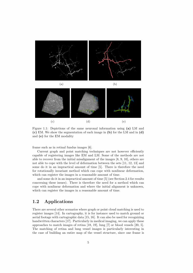
Our main motivation for using graph and point cloud matching approaches liesmostly in medical imaging and mainly in the registration of electron microscopy(EM) and light microscopy (LM) images of neuronal trees (see Fig. 1.1). Imagesextracted using these techniques have generally a very low level of similarity intexture between each other. These images also present very different resolutions– the resolution of a good LM is about 300 nm and the one of an EM can fallbelow 1 Angstrom (reaching a subatomic level) [1, 2] – in our data it is a fewnm. Although the EM images give us a better resolution of the observed tissue,the LM images help us obtain a bigger picture of the neuronal network, andtherefore it is useful to register them. There are several other applications whichpresent similar difficulties in medical imaging where similar vessel tree or graph-like structures are present, such as registering images of brain blood vesselsacquired with different modalities – two photon microscopy and bright-fieldoptical microscopy (see Fig. 1.2). Other applications are discussed in Section 1.2.
A typical approach for image registration is to match image informationusing texture or intensity information [3], optimizing the matching defining anenergy criterion and finding its minimum. Some algorithms make use of imagedescriptors, such as SIFT descriptors or salient feature regions [4], in order tofind key features within images enabling a faster matching, sometimes invariantto properties like rotation and scale. However, a lot of image information isnot used and finding feature points might be difficult in some kind of images.Nonetheless, this is not possible whenever the images to be registered lookvery different, and such is the case when registering EM and LM images (seeFig. 1.1). Another problem which feature-based approaches have in this kind ofapplication is that the structures within the same image do not have distinctivefeatures and are locally similar. In order to surpass these difficulties, a differentapproach is to segment the structures present on the images, followed by thematching of those structures based on their geometric properties [5, 6, 7]. Usinggraph or point cloud matching can therefore allow for a solution for registeringimages acquired with different modalities, as well as acquired at different timepoints such as in angiography [5] or where only a subset of the structure iscommon between the two images since they cannot be entirely acquired in one
4
(a) (b)
(c) (d) (e)
Figure 1.1: Depictions of the same neuronal information using (a) LM and(c) EM. We show the segmentation of each image in (b) for the LM and in (d)and (e) for the EM modality
frame such as in retinal fundus images [6].
Current graph and point matching techniques are not however efficientlycapable of registering images like EM and LM. Some of the methods are notable to recover from the initial misalignment of the images [8, 9, 10], others arenot able to cope with the level of deformation between the sets [11, 12, 13] andsome do it in an impractical amount of time [5]. There is therefore the needfor rotationally invariant method which can cope with nonlinear deformation,which can register the images in a reasonable amount of time.
and some do it in an impractical amount of time [5] (see Section 2.4 for resultsconcerning these issues). There is therefore the need for a method which cancope with nonlinear deformation and where the initial alignment is unknown,which can register the images in a reasonable amount of time.
1.2 Applications
There are several other scenarios where graph or point cloud matching is used toregister images [14]. In cartography, it is for instance used to match ground oraerial footage with cartographic data [15, 16]. It can also be used for recognizinghandwritten characters [17]. Particularly in medical imaging, we can apply theseapproaches to match images of retina [18, 19], lung [7] or blood vessels [20, 5].The matching of retina and lung vessel images is particularly interesting inthe case of building an entire map of the vessel structure, since one frame is
5
(a) (b) (c) (d)
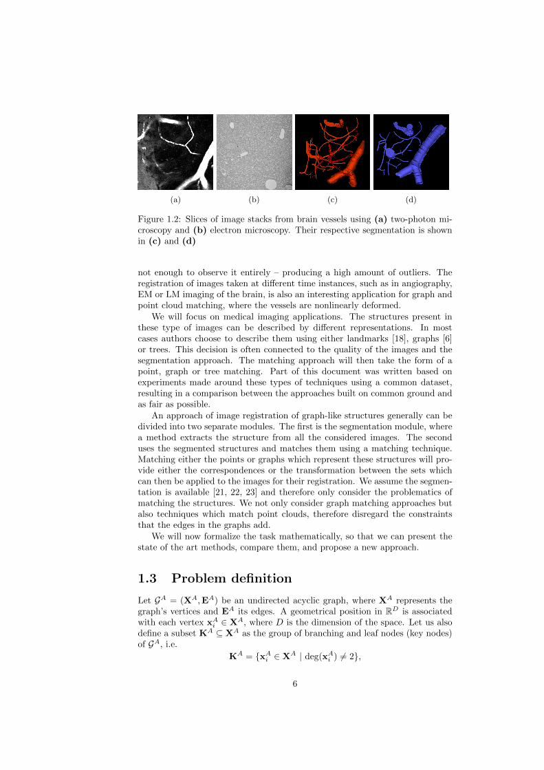
Figure 1.2: Slices of image stacks from brain vessels using (a) two-photon mi-croscopy and (b) electron microscopy. Their respective segmentation is shownin (c) and (d)
not enough to observe it entirely – producing a high amount of outliers. Theregistration of images taken at different time instances, such as in angiography,EM or LM imaging of the brain, is also an interesting application for graph andpoint cloud matching, where the vessels are nonlinearly deformed.
We will focus on medical imaging applications. The structures present inthese type of images can be described by different representations. In mostcases authors choose to describe them using either landmarks [18], graphs [6]or trees. This decision is often connected to the quality of the images and thesegmentation approach. The matching approach will then take the form of apoint, graph or tree matching. Part of this document was written based onexperiments made around these types of techniques using a common dataset,resulting in a comparison between the approaches built on common ground andas fair as possible.
An approach of image registration of graph-like structures generally can bedivided into two separate modules. The first is the segmentation module, wherea method extracts the structure from all the considered images. The seconduses the segmented structures and matches them using a matching technique.Matching either the points or graphs which represent these structures will pro-vide either the correspondences or the transformation between the sets whichcan then be applied to the images for their registration. We assume the segmen-tation is available [21, 22, 23] and therefore only consider the problematics ofmatching the structures. We not only consider graph matching approaches butalso techniques which match point clouds, therefore disregard the constraintsthat the edges in the graphs add.
We will now formalize the task mathematically, so that we can present thestate of the art methods, compare them, and propose a new approach.
1.3 Problem definition
Let GA = (XA,EA) be an undirected acyclic graph, where XA represents thegraph’s vertices and EA its edges. A geometrical position in RD is associatedwith each vertex xAi ∈ XA, where D is the dimension of the space. Let us alsodefine a subset KA ⊆ XA as the group of branching and leaf nodes (key nodes)of GA, i.e.
KA = {xAi ∈ XA | deg(xAi ) 6= 2},
6
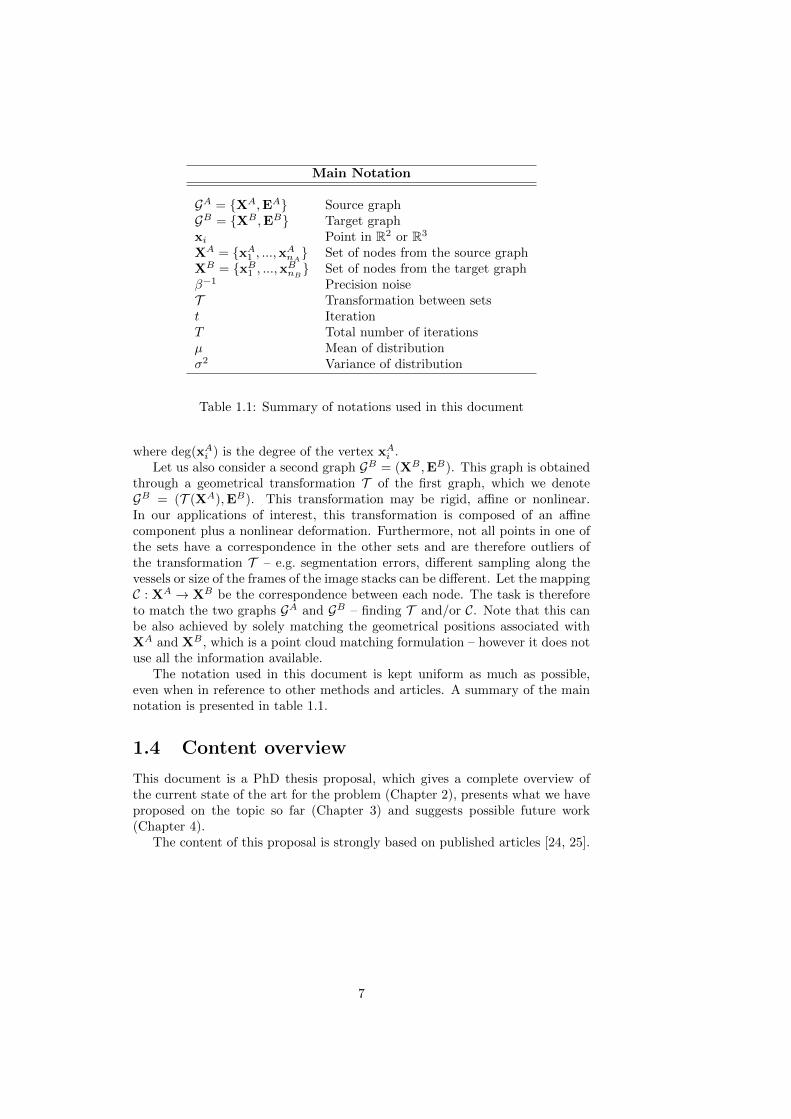
Main Notation
GA = {XA,EA} Source graphGB = {XB ,EB} Target graphxi Point in R2 or R3
XA = {xA1 , ...,xAnA} Set of nodes from the source graphXB = {xB1 , ...,xBnB} Set of nodes from the target graphβ−1 Precision noiseT Transformation between setst IterationT Total number of iterationsµ Mean of distributionσ2 Variance of distribution
Table 1.1: Summary of notations used in this document
where deg(xAi ) is the degree of the vertex xAi .Let us also consider a second graph GB = (XB ,EB). This graph is obtained
through a geometrical transformation T of the first graph, which we denoteGB = (T (XA),EB). This transformation may be rigid, affine or nonlinear.In our applications of interest, this transformation is composed of an affinecomponent plus a nonlinear deformation. Furthermore, not all points in one ofthe sets have a correspondence in the other sets and are therefore outliers ofthe transformation T – e.g. segmentation errors, different sampling along thevessels or size of the frames of the image stacks can be different. Let the mappingC : XA → XB be the correspondence between each node. The task is thereforeto match the two graphs GA and GB – finding T and/or C. Note that this canbe also achieved by solely matching the geometrical positions associated withXA and XB , which is a point cloud matching formulation – however it does notuse all the information available.
The notation used in this document is kept uniform as much as possible,even when in reference to other methods and articles. A summary of the mainnotation is presented in table 1.1.
1.4 Content overview
This document is a PhD thesis proposal, which gives a complete overview ofthe current state of the art for the problem (Chapter 2), presents what we haveproposed on the topic so far (Chapter 3) and suggests possible future work(Chapter 4).
The content of this proposal is strongly based on published articles [24, 25].
7
Chapter 2
State of the art
2.1 Overview
Point cloud and graph matching techniques for image registration have been onfocus for several years [14, 26, 27]. We will focus on matching points or graphsassociated with geometrical positions, although some of the methods are alsoused for feature matching. State of the art approaches can generally be dividedinto three classes.
The first assumes the transformation between the points is almost rigid oraffine, and therefore can be tested using few number of points. Methods likeRANSAC [11] and its variants [28, 29, 27] use this properties to hypothesizerandom correspondences, evaluating each test until a good score has been found.Some of the methods then expands every good hypothesis, looking for a morerobust solution [29, 30]. Although it works well on sets of a few points wherethe transformation between them is mostly rigid or affine, it struggles with alarge number of points and on sets transformed non rigidly.
The second class of points formalizes the task as an optimization problemwhere the task is to find the transformation T which minimizes the distancebetween the sets, where both the parametrization of T and the optimizationalgorithm is considered differently in most approaches. The point clouds can befor example considered to be transformed rigidly [31], by Thin-plate splines [10],or by a Gaussian mixture model [8]. These techniques require a good initialalignment, since large transformations such as with a high rotation are usuallytoo far in the objective function space.
The third class of approaches computes pairwise compatibilities betweenthe points or nodes, based on properties of the geometrical space between thepoints or the graph’s connectivity when graphs are considered. Some of theseapproaches formalize the task as a quadratic program [6, 32], which is becomesimpractical when working with larger sets of points. A few techniques were pre-sented to decrease the time complexity issue [33, 12, 34], however since the prob-lem is many times non-convex, the solution can tend a local minimum. It is alsopossible to formalize the similarities as direct similarities between nodes [35],looking for example for the distribution of points between the neighborhood ofeach point. These techniques are however sensitive when the transformationbetween the points is nonlinear.
8
In this chapter, we present a comparison between some of the state of theart methods for graph and point cloud matching, consisting of their detaileddescription, the description of the datasets used in their comparison and theconsequent results. These results are also presented in [25]. We will show thatthere is a need for a new approach, invariant to rotation, robust to nonlineardeformation, which can run in practical time complexity. The tested methodsincluded in this document were the following:
- Point matching
– Coherent Point Drift (CPD) [8]
– Iterative Closest Point (ICP) [31]
– Iterative Closest Reciprocal Point (ICRP) [36]
– Thin-plate spline - robust point matching (TPS) [10]
– Random Sample Consensus (RANSAC) [11]
– Shape Context (SHAPEC) [35]
- Graph matching
– Spectral Matching with Affine Constraints (SMAC) [32]
– A Path Following Algorithm (PATH) [12]
We will now describe each of the methods, which we used in our experimentsto evaluate the state of the art.
2.2 Point cloud matching
2.2.1 RANSAC
RANSAC was first presented in 1981 [11], and it is a method for fitting a modelto experimental data, which in our case is the transformation between the setsof points.
The approach selects s sample points in each iteration t from both pointclouds XA and XB , which we are going to refer to as xA(t) and xB(t). We thencalculate the affine transformation T(t) between these two set of points. Thetype transformation to use in the fitting is one of the parameters to be chosen.We then fit this transformation to all the points T(t)(xB) = T(t).xB , and counthow many inliers this transformation computes. We do this by counting howmany points in T(t)(xB) have at least one point of xA at a distance of at mostβ−1, to which we refer as inliers. The transformation which produces the mostinliers is the output of the approach.
The total number of iterations that is required to have a probability of p offinding the optimal solution is estimated as
T =log (1− p)
log (1− pts), (2.1)
where pt is the percentage of inliers obtained with transformation T(t) at iter-ation t. T is updated when the method finds the highest number of inliers sofar.
9
2.2.2 TPS
The TPS-RPM algorithm was introduced in 2003 [10], in a paper co-authored byone of the authors of the softassign algorithm [37]. The method presents many ofthe ideas of previous work, such as the correspondence matrix with an extra rowand column to identify outliers and a very similar objective function to minimize.A new entropy term T
∑nAi=1
∑nBj=1mij logmij is introduced into the criterion,
where T is called a temperature parameter and the remaining variables aredefined as in softassign. As the algorithm iterates, the temperature is reduced,controlling the level of convexity of the objective function. The g(T ) functionis replaced by a new operator L, with g(T ) = −||LT ||2, which is referred to asa smoothness measure. The objective function to be minimized is then
nA∑i=1
nB∑j=1
mij ||xBj − T (xAi )||2 + λ||LT ||2 + TnA∑i=1
nB∑j=1
mij logmij − ζnA∑i=1
nB∑j=1
mij
(2.2)where ζ is a parameter that weighs the robustness control term. The methodalso analyses a non-rigid case represented by a function
T (XB , A,w) = XB ·A+ φ(XB) · w, (2.3)
where A represents a (D + 1)× (D + 1) affine transformation matrix, where Dis the number of dimensions, w is a K × (D+ 1) warping coefficient matrix andeach φ(XB) is a 1 × nB vector of thin plate splines basis functions, φb(X
B) =||xBb −XB ||2 log ||xBb −XB || for b = 1, ..., nB . With this notation it is possibleto represent non-rigid transformations.
2.2.3 CPD
In 2010, Myronenko and Song presented an alignment technique for rigid, affineand non-rigid transformation cases, called Coherent Point Drift [8]. The authorslook at the task as a probability density estimation problem, with one of thesets being data points XA = (xA1 , ...,x
AnA)T , and the second one representing
Gaussian Mixture Model (GMM) centroids XB = (xB1 , ...,xBnB )T . The GMM
probability density is therefore
p(xA) =
nB+1∑m=1
P (m)p(xA|m), (2.4)
where
P (m) =
{(1− ω) · 1/nB if m 6= nB + 1
ω · 1/nA if m = nB + 1,
p(xA|m) =1
(2πσ2)D/2exp−
||xA−xBm||2
2σ2 ,
and where σ2 is the variance for all GMM components, D the number of dimen-sions and ω the weight for uniform distribution for nB +1, with 0 ≤ ω ≤ 1. Theadded nB + 1 accounts for outliers and noise present in the task. The objectivefunction is the negative log-likelihood, leading to
10
Q(θ, σ2) =1
2σ2
nA∑n=1
nB∑m=1
P (m|xAn )||xAn − T (xBm, θ)||2
+D
2
nA∑n=1
nB∑m=1
P (m|xAn ) log σ2 (2.5)
where T (xBm, θ) is the transformation of the point xBm using parameters θ.An expectation maximization algorithm is used. In the E-step, the values
for P (m|xA) are reassigned and normalized. In the M-step, the transformation’sparameters and the variance of the density functions are updated, using the newvalue for P .
The article goes on to describe different and more detailed approaches tocalculate T (xBm, θ) for the rigid and affine cases. In the rigid case, the transfor-mation is represented by a rotation matrix R and a scaling parameter s togetherwith a translation vector τ , i.e. T (xBm;R, τ, s) = sRxBm + τ . For the affine case,the transformation is represented by a general transformation matrix B and atranslation vector, i.e. T (xBm;B, τ) = BxBm + τ .
A non-rigid approach is also presented. Here, the transformation takes theshape T (XB , v) = XB + v(XB), where v is a displacement function. Theobjective function is changed and a regularization term is added, leading to
Q(v, σ2) =1
2σ2
nA∑n=1
nB∑m=1
P (m|xAn )||xAn − (xBm + v(xBm))||2
+D
2
nA∑n=1
nB∑m=1
P (m|xAn ) log σ2 +λ
2||Lv||2 (2.6)
where λ is a trade-off parameter for regularization and L is a regularizationoperator [38]. Taking a derivative w.r.t. v and equaling it to zero, we getequations for the minimum. The non-linear transformation turns out to beT (XB , v(XB)) = T (XB ,W ) = XB + GW , where G is an nB × nB matrix
with elements gij = e−12 ||
xBi −xBjβ || and W is an nB × D matrix with elements
wm = 1σ2λ
∑nAn=1 P (m|xAn )(xAn −(xBm+v(xBm))). The value for σ2 is also trivially
obtained by deriving the Q function. The algorithm is similar as in the affineand rigid cases.
2.2.4 ICP
The Iterative Closest Point is a very popular method and was first presented in1992 by Besl and McKay [31]. In the method’s own notation, the task is to finda transformation with which the data points XA can fit the model points XB .The method finds the closest point in XB for each point of XA, denoted Y inan operation denominated C(XB
(t),XA), i.e.
Y(t) = C(XB(t),X
A). (2.7)
For each iteration t, a set of points Y(t) is computed as C(XB(t),X
A). The
algorithm then uses quaternion representation (although it can be extended to
11
allow other types of transformations) to obtain the transformation between XB(0)
and Y(t) described by a vector ~q(t). This transformation is applied to XB(0) to
obtain a new set of points, i.e. XB(t+1) = ~q(t)(X
B(0)). These steps are performed
repeatedly until the difference between the mean squared points matching errors(between XA and XB
(t)) for subsequent iterations d(t) and d(t+1) falls bellow athreshold τ .
2.2.5 ICRP
The Iterative Closest Reciprocal Point [36] algorithm is similar ICP, as thename implies. To improve robustness, the method only considers points whichare reciprocally the closest points between the two sets.
2.2.6 SHAPEC
Shape Matching using Shape Context (SHAPEC) was proposed by Belongieet al. [35] and builds a local description for each point of each cloud. Thisdescription is composed of a histogram of neighbor points, where the bins aredistributed depending on the angle and Euclidean distance between points –nθ bins for different angles and nd bins for Euclidean distance to the consid-ered point. The similarity wij between two points xAi and xBj is the absolutedifference between the number of elements in each bin of each histogram.
This formulation allows for some nonlinearity, however it is variant to rota-tion, scale and shearing.
The assignment H with elements hi between points is obtained by applyingthe Hungarian algorithm to a matrix W of similarities wij between the pointsin both sets, such that the energy function
E(H) =
nA∑i=1
hiwij (2.8)
is minimized.
2.3 Graph matching
2.3.1 SMAC
The paper presented in 2006 by Cour et al. [32], introduces a technique namedSMAC where two graphs GA = (XA,EA,AA) and GB = (XB ,EB ,AB) arematched. The method tries to obtain the mapping between the vertices XA
and XB and consequently also EA and EB , based on edge attributes AA,ABgathered from the edges EA and EB .
The method builds a compatibility matrix W with the size nAnB × nAnBwhere each entry describes the compatibility between two edges of the twographs – Wii′,jj′ = f(Aij ,Ai′j′) where ij ∈ EA and i′j′ ∈ EB .
Having built this matrix W , the method needs to correctly assign the cor-respondences between edges of opposite graphs. Since the task is NP-complete,the proposed algorithm finds an approximate solution by Spectral Matching[33]. In summary, this method considers solely the edge information to matchgraphs, which is positive for situations where the Euclidean distance between
12
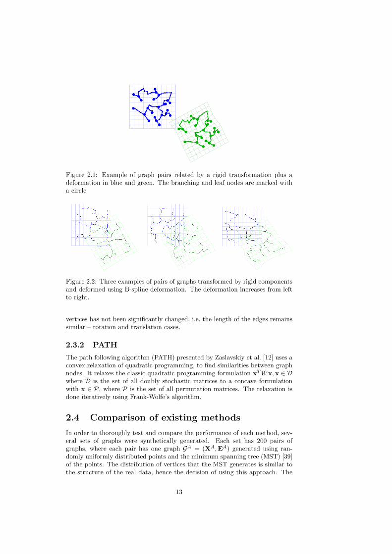
Figure 2.1: Example of graph pairs related by a rigid transformation plus adeformation in blue and green. The branching and leaf nodes are marked witha circle
Figure 2.2: Three examples of pairs of graphs transformed by rigid componentsand deformed using B-spline deformation. The deformation increases from leftto right.
vertices has not been significantly changed, i.e. the length of the edges remainssimilar – rotation and translation cases.
2.3.2 PATH
The path following algorithm (PATH) presented by Zaslavskiy et al. [12] uses aconvex relaxation of quadratic programming, to find similarities between graphnodes. It relaxes the classic quadratic programming formulation xTWx,x ∈ Dwhere D is the set of all doubly stochastic matrices to a concave formulationwith x ∈ P, where P is the set of all permutation matrices. The relaxation isdone iteratively using Frank-Wolfe’s algorithm.
2.4 Comparison of existing methods
In order to thoroughly test and compare the performance of each method, sev-eral sets of graphs were synthetically generated. Each set has 200 pairs ofgraphs, where each pair has one graph GA = (XA,EA) generated using ran-domly uniformly distributed points and the minimum spanning tree (MST) [39]of the points. The distribution of vertices that the MST generates is similar tothe structure of the real data, hence the decision of using this approach. The
13
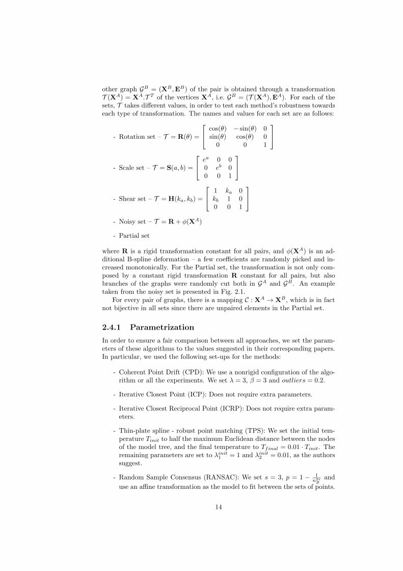
other graph GB = (XB ,EB) of the pair is obtained through a transformationT (XA) = XA.T T of the vertices XA, i.e. GB = (T (XA),EA). For each of thesets, T takes different values, in order to test each method’s robustness towardseach type of transformation. The names and values for each set are as follows:
- Rotation set – T = R(θ) =
cos(θ) − sin(θ) 0sin(θ) cos(θ) 0
0 0 1
- Scale set – T = S(a, b) =
ea 0 00 eb 00 0 1
- Shear set – T = H(ka, kb) =
1 ka 0kb 1 00 0 1
- Noisy set – T = R + φ(XA)
- Partial set
where R is a rigid transformation constant for all pairs, and φ(XA) is an ad-ditional B-spline deformation – a few coefficients are randomly picked and in-creased monotonically. For the Partial set, the transformation is not only com-posed by a constant rigid transformation R constant for all pairs, but alsobranches of the graphs were randomly cut both in GA and GB . An exampletaken from the noisy set is presented in Fig. 2.1.
For every pair of graphs, there is a mapping C : XA → XB , which is in factnot bijective in all sets since there are unpaired elements in the Partial set.
2.4.1 Parametrization
In order to ensure a fair comparison between all approaches, we set the param-eters of these algorithms to the values suggested in their corresponding papers.In particular, we used the following set-ups for the methods:
- Coherent Point Drift (CPD): We use a nonrigid configuration of the algo-rithm or all the experiments. We set λ = 3, β = 3 and outliers = 0.2.
- Iterative Closest Point (ICP): Does not require extra parameters.
- Iterative Closest Reciprocal Point (ICRP): Does not require extra param-eters.
- Thin-plate spline - robust point matching (TPS): We set the initial tem-perature Tinit to half the maximum Euclidean distance between the nodesof the model tree, and the final temperature to Tfinal = 0.01 · Tinit. Theremaining parameters are set to λinit1 = 1 and λinit2 = 0.01, as the authorssuggest.
- Random Sample Consensus (RANSAC): We set s = 3, p = 1 − 1n2sB
and
use an affine transformation as the model to fit between the sets of points.
14
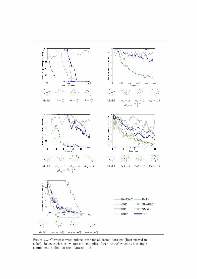
Model θ = π6
θ = 2π6
θ = 3π6
Model scg = .1 scg = .2 scg = .25
scg = |a|+|b|2
Model shg = .2 shg = .4 shg = .8 Model Def.= 5 Def.= 10 Def.= 15
shg = |ka|+|kb|2
Model out = 20% out = 40% out = 60%
Figure 2.3: Correct correspondence rate for all tested datasets (Best viewed incolor). Below each plot, we present examples of trees transformed by the singlecomponent studied on each dataset 15
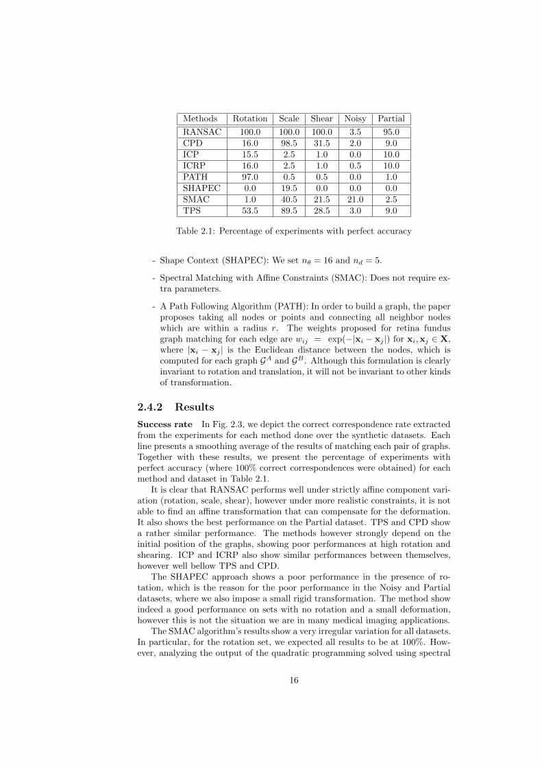
Table 2.1: Percentage of experiments with perfect accuracy
- Shape Context (SHAPEC): We set nθ = 16 and nd = 5.
- Spectral Matching with Affine Constraints (SMAC): Does not require ex-tra parameters.
- A Path Following Algorithm (PATH): In order to build a graph, the paperproposes taking all nodes or points and connecting all neighbor nodeswhich are within a radius r. The weights proposed for retina fundusgraph matching for each edge are wij = exp(−|xi − xj |) for xi,xj ∈ X,where |xi − xj | is the Euclidean distance between the nodes, which iscomputed for each graph GA and GB . Although this formulation is clearlyinvariant to rotation and translation, it will not be invariant to other kindsof transformation.
2.4.2 Results
Success rate In Fig. 2.3, we depict the correct correspondence rate extractedfrom the experiments for each method done over the synthetic datasets. Eachline presents a smoothing average of the results of matching each pair of graphs.Together with these results, we present the percentage of experiments withperfect accuracy (where 100% correct correspondences were obtained) for eachmethod and dataset in Table 2.1.
It is clear that RANSAC performs well under strictly affine component vari-ation (rotation, scale, shear), however under more realistic constraints, it is notable to find an affine transformation that can compensate for the deformation.It also shows the best performance on the Partial dataset. TPS and CPD showa rather similar performance. The methods however strongly depend on theinitial position of the graphs, showing poor performances at high rotation andshearing. ICP and ICRP also show similar performances between themselves,however well bellow TPS and CPD.
The SHAPEC approach shows a poor performance in the presence of ro-tation, which is the reason for the poor performance in the Noisy and Partialdatasets, where we also impose a small rigid transformation. The method showindeed a good performance on sets with no rotation and a small deformation,however this is not the situation we are in many medical imaging applications.
The SMAC algorithm’s results show a very irregular variation for all datasets.In particular, for the rotation set, we expected all results to be at 100%. How-ever, analyzing the output of the quadratic programming solved using spectral
16
Figure 2.4: Time complexity
matching, we conclude that in most cases in which the approach fails, the algo-rithm falls into some local maximum, and that the correct solution has a higherfunction value that the one obtained. In other cases, local symmetry betweenbranches can allow for correspondences to be swapped, since the function valueis the same for both cases.
The PATH approach presents as expected an invariability towards rotation,however the way it builds the graph based in Euclidean distances makes itvariant to small differences in scale, shear, missing nodes and also deformation.
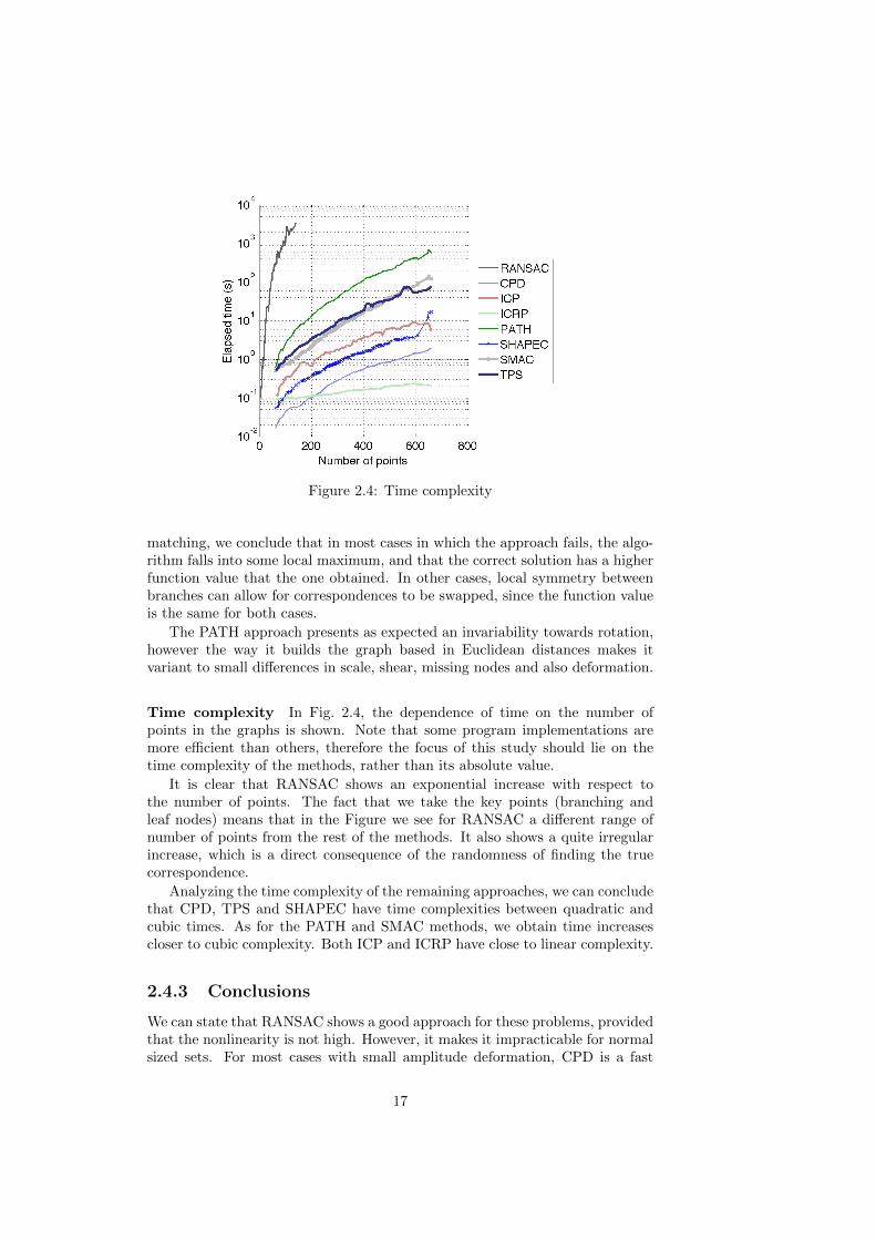
Time complexity In Fig. 2.4, the dependence of time on the number ofpoints in the graphs is shown. Note that some program implementations aremore efficient than others, therefore the focus of this study should lie on thetime complexity of the methods, rather than its absolute value.
It is clear that RANSAC shows an exponential increase with respect tothe number of points. The fact that we take the key points (branching andleaf nodes) means that in the Figure we see for RANSAC a different range ofnumber of points from the rest of the methods. It also shows a quite irregularincrease, which is a direct consequence of the randomness of finding the truecorrespondence.
Analyzing the time complexity of the remaining approaches, we can concludethat CPD, TPS and SHAPEC have time complexities between quadratic andcubic times. As for the PATH and SMAC methods, we obtain time increasescloser to cubic complexity. Both ICP and ICRP have close to linear complexity.
2.4.3 Conclusions
We can state that RANSAC shows a good approach for these problems, providedthat the nonlinearity is not high. However, it makes it impracticable for normalsized sets. For most cases with small amplitude deformation, CPD is a fast
17
approach with good results. However, in cases with high rotation or wheresome nodes are missing, the method fails.
Analyzing the results, we can conclude that there is a need for a new method,which can solve cases with unknown rotation, high deformation and with missingnodes – this is the case of applications such as registering EM and LM images.
18
Chapter 3
Active Testing Search
3.1 Overview
In this chapter, we present the work described in [24]. We consider the problemof point-cloud to point-cloud (PTP) matching. The problem consists of findingcorrespondences between two populations of points, related by a geometricaltransformation. The transformation is assumed to be non-linear but not farfrom affine. The correspondences can be partial. We do not require an initialalignment nor any additional information except the point coordinates. How-ever, if such information is available (e.g. local appearance or connectivity), itcan be incorporated to reduce the search problem.
The main difficulty of the PTP problem is the large set of possible matches.The major challenge lies in the ability to formulate a search procedure thatis tractable and still provides an acceptable solution. This is particularly truewhen the transformation between the two populations is non-rigid.
We consider this problem in the context of medical image registration. Threeimportant challenges lie in such registration tasks. First, the transformationbetween curvilinear structures is generally non-rigid, which induces complexsolutions that are difficult to compute. Second, appearance based measuresof similarity (e.g. key point descriptors) cannot be used in some cases due tothe fact that registration may be between different modalities (e.g. ElectronMicroscopy (EM) and Light Microscopy (LM)) [5]. Finally, registration may beat different physical scales (e.g. nm and µm) and hence consists of registeringone domain to a substructure of another much larger structure.
In our approach, Active Testing Search (ATS) we take a Bayesian pointof view and consider the correspondences to be random. We use a sensor:a black box function, which scores the quality any set of partial or completepoint correspondences. The probability of the correctness of the match givena sensor output is given by a sensor model, which we learn from data. We makeobservations sequentially and integrate information received from the sensorby computing the posterior probability of the correspondence correctness. Weexplore the space of possible potential correspondences by performing a prioritysearch based on the information gain, adding one point match per step, similarto the Twenty Questions game with noisy outputs [40, 41, 42, 43].
19
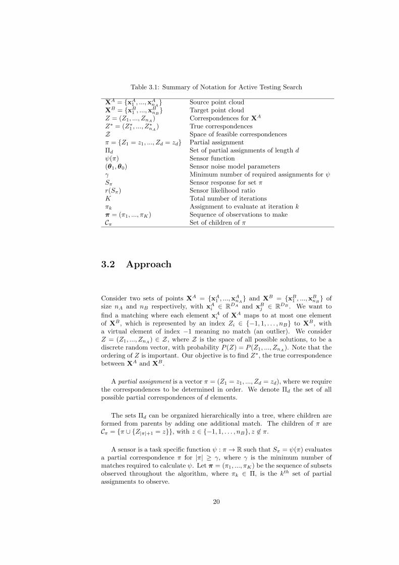
Table 3.1: Summary of Notation for Active Testing Search
XA = {xA1 , ...,xAnA} Source point cloudXB = {xB1 , ...,xBnB} Target point cloudZ = (Z1, ..., ZnA) Correspondences for XA
Z∗ = (Z∗1 , ..., Z∗nA) True correspondences
Z Space of feasible correspondencesπ = {Z1 = z1, ..., Zd = zd} Partial assignmentΠd Set of partial assignments of length dψ(π) Sensor function(θ1,θ0) Sensor noise model parametersγ Minimum number of required assignments for ψSπ Sensor response for set πr(Sπ) Sensor likelihood ratioK Total number of iterationsπk Assignment to evaluate at iteration kπ = (π1, ..., πK) Sequence of observations to makeCπ Set of children of π
3.2 Approach
Consider two sets of points XA = {xA1 , ...,xAnA} and XB = {xB1 , ...,xBnB} ofsize nA and nB respectively, with xAi ∈ RDA and xBj ∈ RDB . We want to
find a matching where each element xAi of XA maps to at most one elementof XB , which is represented by an index Zi ∈ {−1, 1, . . . , nB} to XB , witha virtual element of index −1 meaning no match (an outlier). We considerZ = (Z1, ..., ZnA) ∈ Z, where Z is the space of all possible solutions, to be adiscrete random vector, with probability P (Z) = P (Z1, ..., ZnA). Note that theordering of Z is important. Our objective is to find Z∗, the true correspondencebetween XA and XB .
A partial assignment is a vector π = (Z1 = z1, ..., Zd = zd), where we requirethe correspondences to be determined in order. We denote Πd the set of allpossible partial correspondences of d elements.
The sets Πd can be organized hierarchically into a tree, where children areformed from parents by adding one additional match. The children of π areCπ = {π ∪ {Z|π|+1 = z}}, with z ∈ {−1, 1, . . . , nB}, z 6∈ π.
A sensor is a task specific function ψ : π → R such that Sπ = ψ(π) evaluatesa partial correspondence π for |π| ≥ γ, where γ is the minimum number ofmatches required to calculate ψ. Let π = (π1, ..., πK) be the sequence of subsetsobserved throughout the algorithm, where πk ∈ Π, is the kth set of partialassignments to observe.
20
3.3 Objective
Our objective is to estimate Z∗ from some observation Sπk . To do this, weconsider solving the MAP,
Z∗ = arg maxz∈Z
P (Z|Sπ1, . . . , SπK ) = arg max
z∈Z{P (Z)P (Sπ1
, . . . , SπK |Z)}
= arg maxz∈Z
{P (Z)
K∏i=1
P (Sπk |Z)
}. (3.1)
Clearly, considering all possible correspondences in π is intractable. MethodsRANSAC [11] and MLESAC [28] can been viewed as solving Eq. 3.1 when πcontains only randomly chosen partial assignments of fixed size (i.e. ∀k, |πk| =const, depending on the number of degrees of freedom of the transformation).
In our approach, we differ from RANSAC and MLESAC in two importantways. First, πk are selected sequentially and on the fly, based on the previousvalues observed from π1, . . . , πk−1. This makes our selection process adaptiveand fully data-driven. Second, to allow maximum flexibility with respect tothe types of possible correspondences (i.e. non-rigid transformations), we let|πk| vary; it will typically increase as the transformation is refined and which isvital for estimating correspondences for non-rigid transformations..
3.4 Active Testing Search
Our method attempts to approximately solve the MAP of Eq. 3.1. To do this,we begin with a prior on Z, observe π1 using our chosen sensor ψ, computethe posterior distribution of Z given the new information, Sπ1
, and select themost promising new set π2 to evaluate based on the posterior distribution. Thisprocess repeats K times and the best correspondence set, defined as the set withthe highest number of inliers, is retained.
3.4.1 Sensor and Sensor Model
As described previously, our sensor is a function ψ : Z → R, with a randomresponse ψ(π) = Sπ. We assume the following model
P (Sπ = sπ|Z) =
{ξ(Sπ = sπ;θd1), if π ⊂ Z∗
ξ(Sπ = sπ;θd0), if π 6⊂ Z∗(3.2)
where d = |π|, ξ(Sπ = sπ;θd1) and ξ(Sπ = sπ;θd0) are respectively the posi-tive and negative distributions and θd1 and θd0 its parameters. We also definelikelihood ratio
r(sπ) =ξ(Sπ = sπ ;θd1)
ξ(Sπ = sπ ;θd0). (3.3)
The sensor score implicitly characterizes the expected geometrical transforma-tions and depends directly on the number of assignments d in π. For simplicity,we will assume ξ(·;θd1) and ξ(·;θd0) to be Gaussian and we will describe in Sec. 3.6how the parameters of these distributions can be obtained from training data.
21
Using the Gaussian Processes non-linear regression (GPR) described in [5],we can estimate the position of a match of a point xAi in XA, which we denotexAi . The GPR models the geometrical transformation as affine with a smallrandom nonlinear component, which is spatially correlated and its amplitude iscontrolled by a parameter σ2
n. Note that the prediction is based on a partialassignment π.
We have used GPR to generate the following two sensors:
Assigned Distance We use the predictions from GPR to define the total costof assigning the points {xAi } to XB
Sπ =
nA∑i=1
nB∑j=1
Hi,j · dist(xAi ,xBj ), (3.4)
where dist(xAi ,xBj ) is the Euclidean distance between xAi and xBj and H is
the optimal assignment matrix computed by the Hungarian algorithm [44] sothat Sπ is minimal. We make use of an assignment so that we penalize situationswhere xAi is positioned solely around a subset of small size of XB .
Number of inliers We also calculate the relative number of points consistentwith the GPR. This is calculated as the ratio over |XA| of the number of pointsin XB which have some point {xAi } closer than σ2
n,
Sπ =|I||XA|
, I ={xBj ∈ XB | ∃xAi ,dist(xBj , x
Ai ) < σ2
n
}. (3.5)
3.4.2 Hierarchical search
In many datasets, we can select a smaller number of important points KA
from all points XA to be matched, KA � XA. For example, in a datasetcreated by segmenting a dendritic tree, the branching points are structurallymore important than points on the edges connecting the branching points.
Our strategy then is to use the sensor Sπ = ψ(π) from (3.4) only on the ‘im-portant’ points KA, for ‘small’ partial matches π where |π| < δ. For partialmatches bigger than δ, we switch to the sensor (3.5) evaluated on the full set ofpoints XA. This allows for a fast search at low depths of the search tree, whichconstitutes most of the evaluated proposals πk, and a more discriminative se-lection at higher depths.
3.4.3 Computing Posterior Probability Distributions
In this setting, aggregating observations can be achieved by using a Bayesianformulation. We can compute the posterior distribution when πk has beenobserved by
P (Z|Sπ1, . . . , Sπk) =
1
C
[r(Sπk)1πk⊂Z + 1πk 6⊂Z
]P (Z|Sπ1 , . . . , Sπk−1
), (3.6)
where
C = r(Sπk)P (πk) + 1− P (πk) (3.7)
22
and r(Sπk) is defined in Eq. 3.3. There are two important aspects of (3.6).First, it is recursive, allowing the posterior P (Z | Sπ1
. . . Sπk) to be computedfrom the previous posterior. This allows online integration of new information.Second, the normalization factor C is independent on Z and can therefore beignored when comparing the likelihood of different hypotheses Z.
3.4.4 Implementation and Algorithm
The search method is given in Algorithm 1. The probabilities P (Z|Sπ1, . . . , Sπk)
are stored in a priority queue Q (line 1). Initially, this queue will hold all the ele-ments of the subspace Πγ with the same likelihood ε = 1/ |Πγ | of being containedin the true set of correspondences (i.e. uniform prior on Z). The priority queueis ordered by the likelihood ε that a partial assignment is correct.
Algorithm 1 Active Testing Search (XA,XB ;K,ψ,θ1,θ0, γ)
2: for k = 1 . . .K do3: {πk, εk} = pop(Q); //choose the most likely πk4: Sπk = ψ(πk)5: for z ∈ Cπk do6: Q← Push(πk ∪ {Z|πk|+1 = z}, εkr(Sπk)/|Cπk |)7: end for8: end for9: return π∗ = arg max{π1,...,πK} Sπk
For each iteration k, we select the partial assignment with the biggest likeli-hood εk. We use the sensor and compute the noisy score Sπk = ψ(πk). At thispoint we must compute the posterior distribution given this new observation.To do this, we first generate children Cπk of πk and insert them into the queueusing (3.6) (line 6). The queue maintains an unnormalized posterior distributionto avoid unnecessary computational costs. This process is repeated K times, atwhich point we return the assignment π∗ which scored the highest. Our methoddoes not perform a breadth-first, or depth-first search as in traditional searchstrategies. Rather, it is an adaptive strategy which allows constant backtrackingand avoids hand-tune pruning of the search space.
3.5 Fine alignment
Depending on the choice of K, Algorithm 1 will find only a subset of all inliers.A fine alignment can be added as a post-processing stage, to identify remaininginliers and if possibly slightly modifies the transformation. An algorithm such asthe coherent point drift [8] is very well suited for this task. We use the approachdescribed in [5], which locally finds assignment of the yet unassigned points bythe Hungarian algorithm [44], using the already assigned points as constraints.The GPR transformation model is updated and the process is iterated untilconvergence.
23
(a) (b) (c)
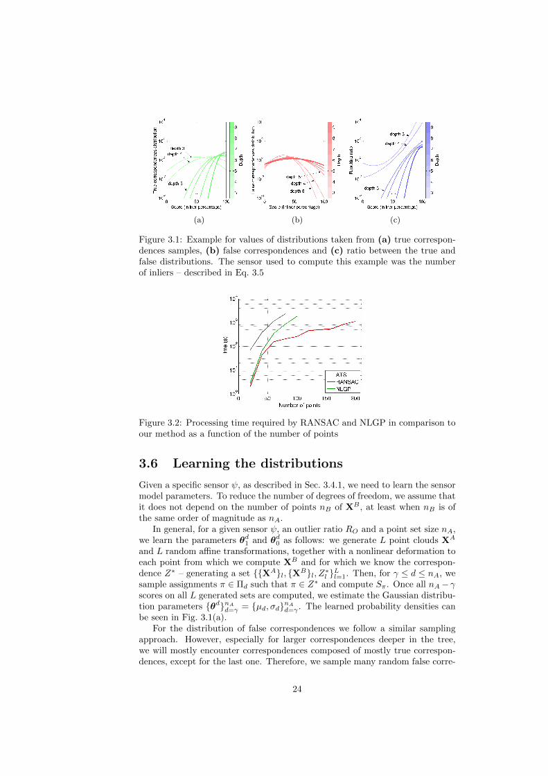
Figure 3.1: Example for values of distributions taken from (a) true correspon-dences samples, (b) false correspondences and (c) ratio between the true andfalse distributions. The sensor used to compute this example was the numberof inliers – described in Eq. 3.5
Figure 3.2: Processing time required by RANSAC and NLGP in comparison toour method as a function of the number of points
3.6 Learning the distributions
Given a specific sensor ψ, as described in Sec. 3.4.1, we need to learn the sensormodel parameters. To reduce the number of degrees of freedom, we assume thatit does not depend on the number of points nB of XB , at least when nB is ofthe same order of magnitude as nA.
In general, for a given sensor ψ, an outlier ratio RO and a point set size nA,we learn the parameters θd1 and θd0 as follows: we generate L point clouds XA
and L random affine transformations, together with a nonlinear deformation toeach point from which we compute XB and for which we know the correspon-dence Z∗ – generating a set {{XA}l, {XB}l, Z∗l }Ll=1. Then, for γ ≤ d ≤ nA, wesample assignments π ∈ Πd such that π ∈ Z∗ and compute Sπ. Once all nA− γscores on all L generated sets are computed, we estimate the Gaussian distribu-tion parameters {θd}nAd=γ = {µd, σd}nAd=γ . The learned probability densities canbe seen in Fig. 3.1(a).
For the distribution of false correspondences we follow a similar samplingapproach. However, especially for larger correspondences deeper in the tree,we will mostly encounter correspondences composed of mostly true correspon-dences, except for the last one. Therefore, we sample many random false corre-
24
(a) (b) (c)
(d) (e)
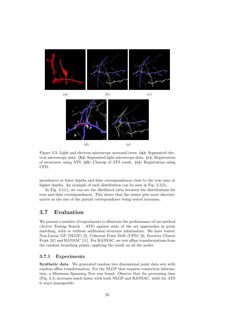
Figure 3.3: Light and electron microscopy neuronal trees. (a): Segmented elec-tron microscopy data. (b): Segmented light microscope data. (c): Registrationof structures using ATS. (d): Closeup of ATS result. (e): Registration usingCPD.
spondences at lower depths and false correspondences close to the true ones athigher depths. An example of such distribution can be seen in Fig. 3.1(b).
In Fig. 3.1(c), we can see the likelihood ratio between the distributions fortrue and false correspondences. This shows that the sensor gets more discrimi-native as the size of the partial correspondence being tested increases.
3.7 Evaluation
We present a number of experiments to illustrate the performance of our method(Active Testing Search – ATS) against state of the art approaches in pointmatching, with or without additional structure information. We have tested:Non-Linear GP (NLGP) [5], Coherent Point Drift (CPD) [8], Iterative ClosestPoint [31] and RANSAC [11]. For RANSAC, we test affine transformations fromthe random branching points, applying the result on all the nodes.
3.7.1 Experiments
Synthetic data We generated random two dimensional point data sets withrandom affine transformation. For the NLGP that requires connection informa-tion, a Minimum Spanning Tree was found. Observe that the processing time(Fig. 2.4) increases much faster with both NLGP and RANSAC, while for ATSit stays manageable.
25
(a) (b) (c) (d)
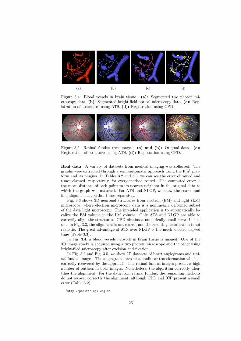
Figure 3.4: Blood vessels in brain tissue. (a): Segmented two photon mi-croscopy data. (b): Segmented bright-field optical microscopy data. (c): Reg-istration of structures using ATS. (d): Registration using CPD.
Figure 3.5: Retinal fundus tree images. (a) and (b): Original data. (c):Registration of structures using ATS. (d): Registration using CPD.
Real data A variety of datasets from medical imaging was collected. Thegraphs were extracted through a semi-automatic approach using the Fiji1 plat-form and its plugins. In Tables 3.2 and 3.3, we can see the error obtained andtimes elapsed, respectively, for every method tested. The computed error isthe mean distance of each point to its nearest neighbor in the original data towhich the graph was matched. For ATS and NLGP, we show the coarse andfine alignment algorithm times separately.
Fig. 3.3 shows 3D neuronal structures from electron (EM) and light (LM)microscopy, where electron microscopy data is a nonlinearly deformed subsetof the data light microscopy. The intended application is to automatically lo-calize the EM volume in the LM volume. Only ATS and NLGP are able tocorrectly align the structures. CPD obtains a numerically small error, but asseen in Fig. 3.3, the alignment is not correct and the resulting deformation is notrealistic. The great advantage of ATS over NLGP is the much shorter elapsedtime (Table 3.3).
In Fig. 3.4, a blood vessels network in brain tissue is imaged. One of the3D image stacks is acquired using a two photon microscope and the other usingbright-filed microscopy after excision and fixation.
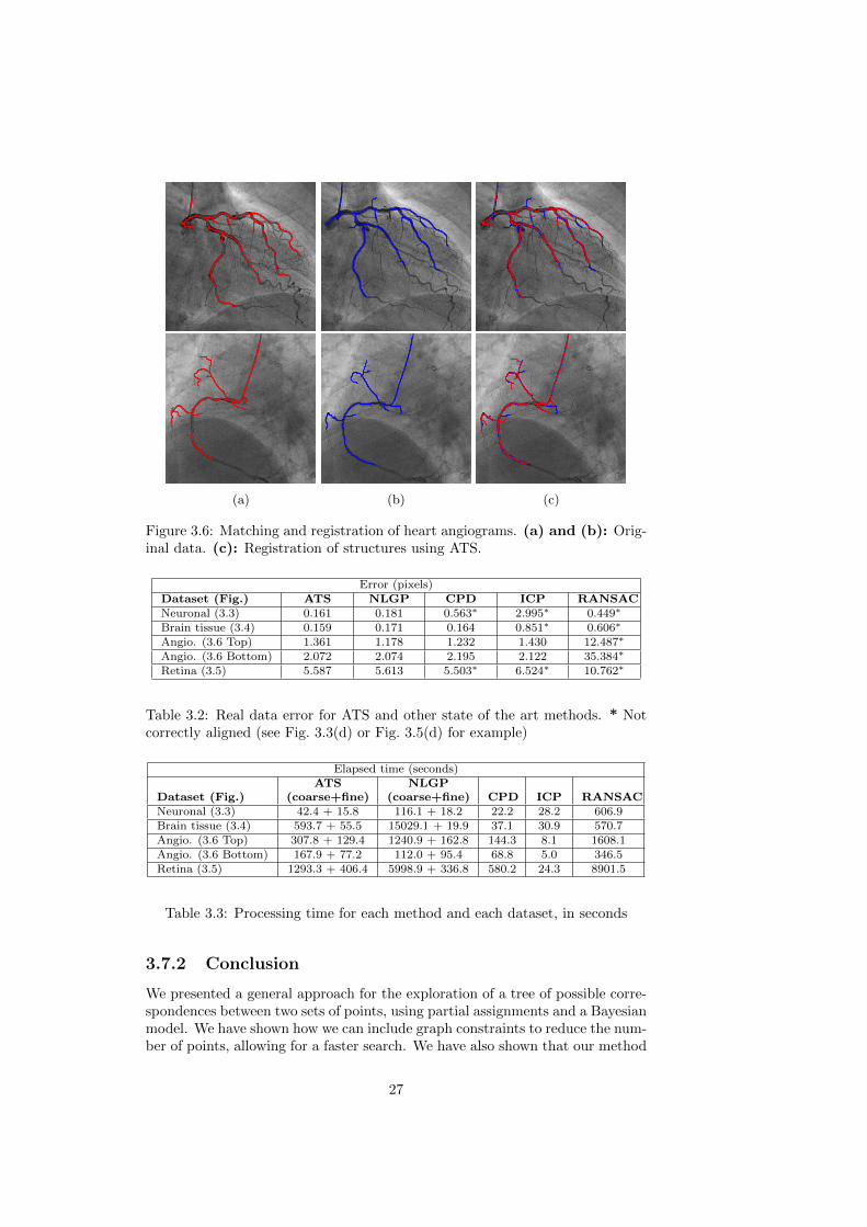
In Fig. 3.6 and Fig. 3.5, we show 2D datasets of heart angiograms and reti-nal fundus images. The angiograms present a nonlinear transformation which iscorrectly recovered by the approach. The retinal fundus images present a highnumber of outliers in both images. Nonetheless, the algorithm correctly iden-tifies the alignment. For the data from retinal fundus, the remaining methodsdo not recover correctly the alignment, although CPD and ICP present a smallerror (Table 3.2).
1http://pacific.mpi-cbg.de
26
(a) (b) (c)
Figure 3.6: Matching and registration of heart angiograms. (a) and (b): Orig-inal data. (c): Registration of structures using ATS.
Table 3.3: Processing time for each method and each dataset, in seconds
3.7.2 Conclusion
We presented a general approach for the exploration of a tree of possible corre-spondences between two sets of points, using partial assignments and a Bayesianmodel. We have shown how we can include graph constraints to reduce the num-ber of points, allowing for a faster search. We have also shown that our method
27
is able to correctly align biological structures that are nonlinearly transformedand extracted with different techniques. These structures need not to be pre-aligned. Our method finds the correct alignment for all considered datasets andis faster than NLGP and RANSAC. It allows a considerably faster explorationof correspondences over the method which correctly finds a solution for harderdatasets.
28
Chapter 4
Future work
4.1 Active Testing Search
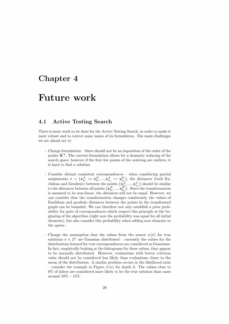
There is more work to be done for the Active Testing Search, in order to make itmore robust and to correct some issues of its formulation. The main challengeswe see ahead are to
- Change formulation – there should not be an imposition of the order of thepoints XA. The current formulation allows for a dramatic reducing of thesearch space, however if the first few points of the ordering are outliers, itis hard to find a solution.
clidean and Geodesic) between the points {xAa1 , ...,xAan} should be similar
to the distances between all points {xBb1 , ...,xBbn}. Since the transformation
is assumed to be non-linear, the distances will not be equal. However, wecan consider that the transformation changes consistently the values ofEuclidean and geodesic distances between the points in the transformedgraph can be bounded. We can therefore not only establish a prior prob-ability for pairs of correspondences which respect this principle at the be-ginning of the algorithm (right now the probability was equal for all initialelements), but also consider this probability when adding new elements tothe queue.
- Change the assumption that the values from the sensor ψ(π) for truesolutions π ∈ Z∗ are Gaussian distributed – currently the values for thedistributions learned for true correspondences are considered as Gaussians.In fact, empirically looking at the histograms for these values, they appearto be normally distributed. However, evaluations with better criterionvalue should not be considered less likely than evaluations closer to themean of the distribution. A similar problem occurs in the likelihood ratio– consider the example in Figure 4.1c) for depth 3. The values close to0% of inliers are considered more likely to be the true solution than casesaround 10%− 15%.
29
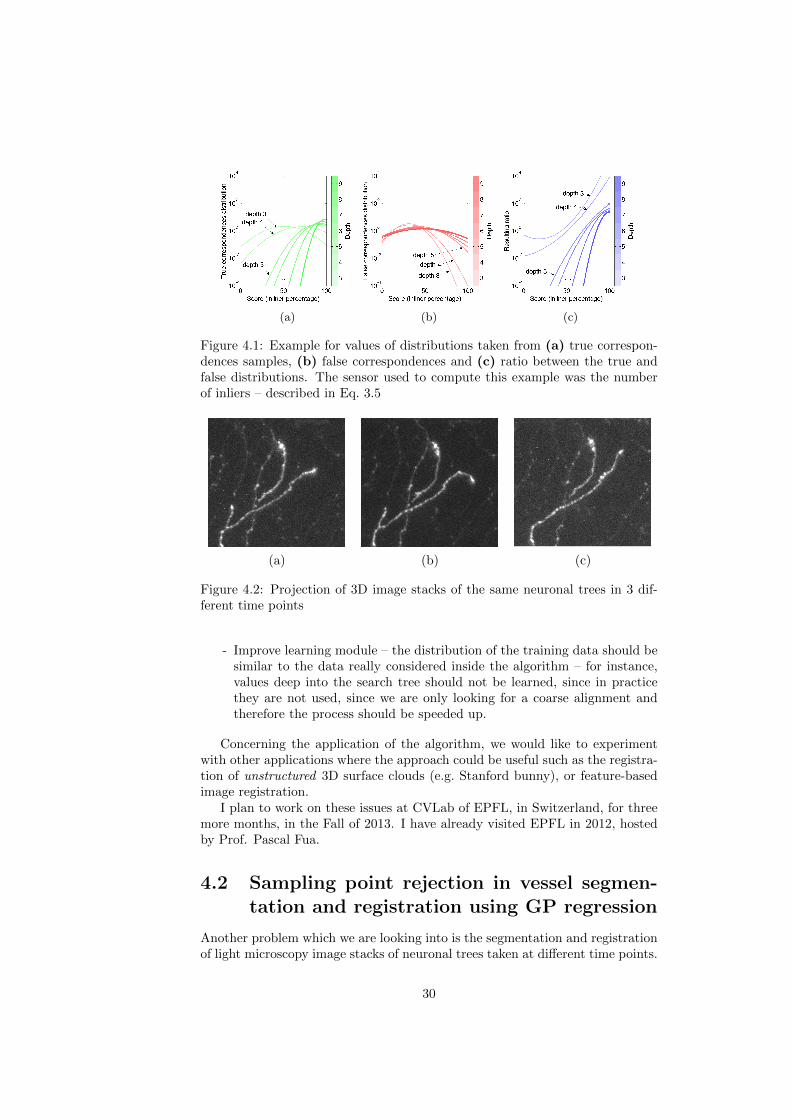
(a) (b) (c)
Figure 4.1: Example for values of distributions taken from (a) true correspon-dences samples, (b) false correspondences and (c) ratio between the true andfalse distributions. The sensor used to compute this example was the numberof inliers – described in Eq. 3.5
(a) (b) (c)
Figure 4.2: Projection of 3D image stacks of the same neuronal trees in 3 dif-ferent time points
- Improve learning module – the distribution of the training data should besimilar to the data really considered inside the algorithm – for instance,values deep into the search tree should not be learned, since in practicethey are not used, since we are only looking for a coarse alignment andtherefore the process should be speeded up.
Concerning the application of the algorithm, we would like to experimentwith other applications where the approach could be useful such as the registra-tion of unstructured 3D surface clouds (e.g. Stanford bunny), or feature-basedimage registration.
I plan to work on these issues at CVLab of EPFL, in Switzerland, for threemore months, in the Fall of 2013. I have already visited EPFL in 2012, hostedby Prof. Pascal Fua.
4.2 Sampling point rejection in vessel segmen-tation and registration using GP regression
Another problem which we are looking into is the segmentation and registrationof light microscopy image stacks of neuronal trees taken at different time points.
30
As it is visible in Fig. 4.2, these trees undergo through some changes during time– in this case between (a) and (b) the brightest vessel on the right bent andbetween (b) and (c) a vessel on the left disappeared. The challenge when doingthe registration of these images is that the trees are highly deformed, there is alot of noise (hard to segment under the same parameters), among others.
Assuming the images are fairly aligned, one can sample points from one ofthe images and use normalized cross correlation around the neighborhood of theremaining images, in order to find matches. Although we are able to find someof the true correspondences accurately, some will be identified incorrectly. Thetype of transformation between sampled points could however be described withthe Gaussian Processes (GP) regression [20], and could help to reject outlierswhich do not follow the same transformation as other points. The GP approachprovides a set of predictions on the projection of one of the sets over the others,given a partial set of assumed correspondences. These predictions are Gaussiansover the position of the projection of each point, which can be interpreted asprobabilities of being a match to the corresponding point.
This idea is still in an early phase, and many other stages are missing.However we believe this could be part of the future work for our research.
31
Bibliography
[1] David B. Williams and C. Barry Carter. The Transmission Electron Mi-croscope. Springer, 2009.
[2] Karen A. Holbrook and George F. Odland. The fine structure of developinghuman epidermis: Light, scanning, and transmission electron microscopyof the periderm. Journal of Investigative Dermatology, 65:16–38, 1975.
[3] Nicola Ritter, Robyn Owens, James Cooper, Robert H. Eikelboom, andPaul P. Van Saarloos. Registration of stereo and temporal images of theretina. IEEE Trans. on Medical Imaging, 18:404–418, 1999.
[4] Jian Zheng, Jie Tian, Yakang Dai, Kexin Deng, and Jian Chen. Retinalimage registration based on salient feature regions. Proceedings of the Inter-national Conference of IEEE Engineering in Medicine and Biology Society,2009:102–105, 2009.
[5] Eduard Serradell, Przemys law G lowacki, Jan Kybic, Francesc Moreno-Noguer, and Pascal Fua. Robust non-rigid registration of 2D and 3D graphs.IEEE CVPR, pages 996–1003, 2012.
[6] Kexin Deng, Jie Tian, Jian Zheng, Xing Zhang, Xiaoqian Dai, and Min Xu.Retinal fundus image registration via vascular structure graph matching.Journal of Biomedical Imaging, 2010:14:1–14:13, January 2010.
[7] Dirk Smeets, Pieter Bruyninckx, Johannes Keustermans, Dirk Vander-meulen, and Paul Suetens. Robust matching of 3d lung vessel trees. InThe Third International Workshop on Pulmonary Image Analysis, pages61–70, 2010.
[8] Andriy Myronenko and Xubo Song. Point set registration: Coherentpoint drift. IEEE Trans. on Pattern Analysis and Machine Intelligence,32(12):2262–2275, 2010.
[9] Bing Jian and B.C. Vemuri. Robust point set registration using gaussianmixture models. Pattern Analysis and Machine Intelligence, IEEE Trans-actions on, 33(8):1633–1645, 2011.
[10] Haili Chui and Anand Rangarajan. A new point matching algorithm fornon-rigid registration. CVIU, 89:114–141, February 2003.
[11] Martin A. Fischler and Robert C. Bolles. Random sample consensus: aparadigm for model fitting with applications to image analysis and auto-mated cartography. Commun. ACM, 24:381–395, 1981.
32
[12] Mikhail Zaslavskiy, Francis Bach, and Jean-Philippe Vert. A path follow-ing algorithm for the graph matching problem. IEEE Trans. on PatternAnalysis and Machine Intelligence, 31(12):2227–42, 2009.
[13] Marius Leordeanu, Martial Hebert, and Rahul Sukthankar. An integerprojected fixed point method for graph matching and map inference. InProceedings Neural Information Processing Systems. Springer, December2009.
[14] Donatello Conte, Pasquale Foggia, Carlo Sansone, and Mario Vento. Thirtyyears of graph matching in pattern recognition. IJPRAI, 18:265–298, 2004.
[15] Mark L. Williams, Richard C. Wilson, and Edwin R. Hancock. Multi-ple graph matching with bayesian inference. Pattern Recognition Letters,18:080, 1997.
[16] Marcus A. Brubaker, Andreas Geiger, and Raquel Urtasun. Lost! leverag-ing the crowd for probabilistic visual self-localization. In IEEE Conf. onComputer Vision and Pattern Recognition (CVPR 2013), Portland, OR,June 2013.
[17] Anand Rangarajan and Eric Mjolsness. A lagrangian relaxation networkfor graph matching. IEEE Trans. on Neural Networks, 7:4629–4634, 1996.
[18] Ali Can, Charles V. Stewart, Badrinath Roysam, and Howard L. Tanen-baum. A feature-based, robust, hierarchical algorithm for registering pairsof images of the curved human retina. IEEE Trans. on Pattern Analysisand Machine Intelligence, 24:347–364, March 2002.
[19] Bin Fang and Yuan Yan Tang. Elastic registration for retinal images basedon reconstructed vascular trees. IEEE Trans. on Biomedical Engineering,53(6):1183–1187, 2006.
[20] Eduard Serradell, Francesc Moreno-Noguer, Jan Kybic, and Pascal Fua.Robust elastic 2D/3D geometric graph matching. SPIE Medical Imaging,8314(1):831408–831408–8, 2012.
[21] Richard Socher, Adrian Barbu, and Dorin Comaniciu. A learning basedhierarchical model for vessel segmentation. In IEEE International Sympo-sium on Biomedical Imaging, pages 1055–1058, 2008.
[22] Dan Claudiu Ciresan, Alessandro Giusti, Luca Maria Gambardella, andJurgen Schmidhuber. Neural networks for segmenting neuronal structuresin em stacks. In Segmentation of Neuronal Structures in EM Stacks Work-shop at International Symposium on Biomedical Imaging, 2012.
[23] Dirk Breitenreicher, Michal Sofka, Stefan Britzen, and Shaohua KevinZhou. Hierarchical discriminative framework for detecting tubular struc-tures in 3d images. In Information Processing in Medical Imaging, pages328–339, 2013.
[24] Miguel Amavel Pinheiro, Raphael Sznitman, Eduard Serradell, Jan Kybic,Francesc Moreno-Noguer, and Pascal Fua. Active testing search for pointcloud matching. In James C. Gee, Sarang Joshi, Kilian M. Pohl, William M.
33
Wells, and Lilla Zollei, editors, Information Processing in Medical Imaging,volume 7917, pages 572–583, Heidelberg, 2013. Springer.
[25] Miguel Amavel Pinheiro. Graph and point cloud registration for tree-likestructures: survey and evaluation. In Libor Husnık, editor, 17th Interna-tional Student Conference on Electrical Engineering, page 144, Technicka2, Prague, Czech Republic, 2013. Czech Technical University in Prague.
[26] Szymon Rusinkiewicz and Marc Levoy. Efficient variants of the ICP al-gorithm. International Conference on 3-D Digital Imaging and Modeling,pages 145–152, 2001.
[27] Sunglok Choi, Taemin Kim, and Wonpil Yu. Performance Evaluation ofRANSAC Family. In British Machine Vision Conference. British MachineVision Association, 2009.
[28] Philip H. S. Torr and Andrew Zisserman. MLESAC: A new robust estima-tor with application to estimating image geometry. Computer Vision andImage Understanding, 78:138–156, 2000.
[29] Ondrej Chum and Jirı Matas. Matching with PROSAC – progressive sam-ple consensus. IEEE CVPR, pages 220–226, 2005.
[30] Karel Lebeda, Jirı Matas, and Ondrej Chum. Fixing the locally optimizedRANSAC. In British Machine Vision Conference, pages 1–11, 2012.
[31] Paul J. Besl and Neil D. McKay. A method for registration of 3-D shapes.IEEE Trans. on Pattern Analysis and Machine Intelligence, 14(2):239–256,1992.
[32] Timothee Cour, Praveen Srinivasan, and Jianbo Shi. Balanced graphmatching. Neural Information Processing Systems, pages 313–320, 2006.
[33] Marius Leordeanu and Martial Hebert. A Spectral Technique for Cor-respondence Problems Using Pairwise Constraints. IEEE ICCV, 2:1482–1489, 2005.
[34] Minsu Cho, Jungmin Lee, and Kyoung Mu Lee. Reweighted random walksfor graph matching. In Proceedings of the 11th European conference onComputer vision: Part V, ECCV’10, pages 492–505, Berlin, Heidelberg,2010. Springer-Verlag.
[35] Serge Belongie, Jitendra Malik, and Jan Puzicha. Shape matching andobject recognition using shape contexts. IEEE Trans. on Pattern Analysisand Machine Intelligence, 24:509–522, 2001.
[36] Tomas Pajdla and Luc Van Gool. Matching of 3-D curves using semi-differential invariants. In IEEE ICCV, pages 390–395, 1995.
[37] Steven Gold, Anand Rangarajan, Chien Ping Lu, and Eric Mjolsness. Newalgorithms for 2D and 3D point matching: Pose estimation and correspon-dence. Pattern Recognition, 31:957–964, 1997.
[38] Zhe Chen and Simon Haykin. On different facets of regularization theory.Neural Computation, 14(12):2791–2846, 2002.
34
[39] Otakar Boruvka. O Jistem Problemu Minimalnım (About a Certain Mini-mal Problem) (in Czech, German summary). Prace Mor. Prırodoved. Spol.v Brne III, 3, 1926.
[40] Donald Geman and Bruno Jedynak. An active testing model for trackingroads in satellite images. IEEE Trans. on Pattern Analysis and MachineIntelligence, 18:1–14, 1995.
[41] Alan L. Yuille and James Coughlan. Twenty questions, focus of atten-tion, and A*: A theoretical comparison of optimization strategies. In In-ternational Workshop on Energy Minimization Methods in CVPR, pages197–212, 1997.
[42] Raphael Sznitman and Bruno Jedynak. Active testing for face detection andlocalization. IEEE Trans. on Pattern Analysis and Machine Intelligence,32(10):1914–1920, 2010.
[43] Raphael Sznitman, Rogerio Richa, Russell H. Taylor, Bruno Jedynak, andGregory D. Hager. Unified detection and tracking of instruments duringretinal microsurgery. IEEE Trans. on Pattern Analysis and Machine In-telligence, 99:1, 2012.
[44] Harold W. Kuhn. The Hungarian method for the assignment problem.Naval Research Logistics, 2(1-2):83–97, 1955.