36
Research report MA12-05 University of Leicester Department of Mathematics 2012
| Date post: | 22-May-2018 |
| Category: |
Documents |
| Upload: | truongnguyet |
| View: | 215 times |
| Download: | 1 times |

Research report
MA12-05
University of Leicester
Department of Mathematics
2012

Math. Model. Nat. Phenom.Vol. X , No. X, 2012, pp. X
Precise self-tuning of spiking patterns in coupled neuronal oscillators
I. Tyukin a,b1, V. Kazantsevc,d
a Department of Mathematics, University of Leicester, University Road, LE1 7RH, UKb Deptartment of Automation and Control Processes, St-Petersburg State University
of Electrical Engineering, Prof. Popova str. 5, 197376, Russiac Department of Nonlinear Dynamics, Institute of Applied Physics of RAS,
Nizhny Novgorod, Russiad Department of Neurodynamics and Neurobiology,
University of Nizhny Novgorod, Nizhny Novgorod, Russia
Abstract. In this work we discuss and analyze spiking patterns in a generic mathematical model oftwo coupled non-identical nonlinear oscillators suppliedwith a spike-timing dependent plasticity(STDP) mechanism. Spiking patterns in the system are shown to converge to a phase-locked statein a broad range of parameters. Precision of the phase locking, i.e. the amplitude of relative phasedeviations from a given reference, depends on the natural frequencies of oscillators and, addition-ally, on parameters of the STDP law. These deviations can be optimized by appropriate tuningof gains (i.e. sensitivity to spike-timing mismatches) of the STDP mechanisms. The deviations,however, can not be made arbitrarily small neither by mere tuning of STDP gains nor by adjust-ing synaptic weights. Thus if accurate phase-locking in thesystem is required then an additionaltuning mechanism is generally needed. We found that adding avery simple adaptation dynamicsin the form of slow fluctuations of the base line in the STDP mechanism enables accurate phasetuning in the system with arbitrary high precision. The scheme applies to systems in which indi-vidual oscillators operate in the oscillatory mode. If the dynamics of oscillators becomes bistablethen relative phase may fail to converge to a given value giving rise to the emergence of complexspiking sequences.
Key words: Nonlinear phase oscillators, spike-timing dependent plasticity, adaptive control, non-linear parametrization, convergence, neural oscillatorsAMS subject classification:92B25, 92C20, 37N25, 37M20
1Corresponding author. E-mail: [email protected]
1

I.Yu. Tyukin, V.B. Kazantsev Precise phase self-tuning of spiking patterns
Introduction
Precise and robust firing activity in neural systems in whichclusters of neurons produce time-lockedspiking sequenceshas recently received substantial attention in the literature [8, 9, 19, 12].Despite inherent variability in the dynamics of individualoscillators, relative time lags betweenspikes in these sequences are robust; the sequences can repeat spontaneously, or they can be gener-ated in response to a certain stimulus. A number of theoretical frameworks have been proposed toexplain emergence and persistence of these precise firing patterns with different inter-spike timing,see e.g. [9] and related notions of synchronized chains (synfire chains) and polychronous groups.In these frameworks spike-timing dependent plasticity (STDP), linked to the post-to-presynaptictiming, is advocated as a mechanism that is directly responsible for the emergence of persistentspike sequences within a given topological substrate.
For a pair of synaptically connected cells, STDP stands for achange in synaptic efficacy as afunction of timing between pre- and post- synaptic events. If the pos-synaptic event occurs withina given interval of time from the onset of the pre-synaptic one then efficacy of synaptic transmis-sion enhances. If, however, the opposite takes place, i.e. apost-synaptic event is followed bypre-synaptic spike, then the efficacy decreases (see Fig. 1). At the level of physical organization,
Figure 1: Phenomenological description of spike-timing dependent plasticity
several factors may affect the efficacy of signal transmission in the cells [7]. They include: distancebetween the synapse and the soma, number of connections between neurons, dynamic regime offiring (such as e.g. bursting, when multiple spikes are transmitted in response to single event),long-term potentiation and depression, presence of chemicals and neurotransmitters, and state ofthe membrane potential relative to the threshold value. At the level of processes, many forms ofSTDP have been discovered to date [22], and a common knowledge is that STDP is supportedby multiple molecular cascades inducing changes in both postsynaptic spines and in presynapticterminals. Calcium flux through NMDA receptors located in spines [15] is an example of mech-anisms directly responsible for postsynaptic changes. In this mechanism, excitatory postsynapticpotentials preceding back-propagating action potentialselicit calcium influx through postsynapticNMDA receptors. Higher calcium concentration, in turn, facilitates evoking of postsynaptic spikesin response to the presynaptic ones. Changes in presynapticterminals are observed, for example,in the hippocampal mossy fiber synapses [16]. STDP-like phenomena can also occur due to themodulation of synaptic transmission by endocannabinoid-mediated retrograde cascades. Thesecascades, once activated, trigger the activation of presynaptic receptors [17, 3].
Large diversity of the ways in which STDP may manifest itselfin empirical observations has
2

I.Yu. Tyukin, V.B. Kazantsev Precise phase self-tuning of spiking patterns
lead to a broad range of mathematical models of the phenomenon. These models, although phe-nomenological, are widely used in computational and theoretical studies (see e.g. [5, 23, 26, 11]).In the majority of these models the principal factor determining synaptic efficacy is the synapticweight. The latter is described by a dynamic variable of which the value changes in responseto post-to-presynaptic spike timing. Increments/decrements of the weights are often associatedwith LTP/LTD respectively. One of the outcomes of such activity-dependent modifications of thesynaptic weights is that connections between individual cells may grow or decay over time by arelatively large amount. This facilitates emergence of neuronal clusters that fire together, up to atolerance margin.
Despite abundance of reports suggesting a possible role of the classical connection-modulatingSTDP in the formation of spiking patterns in networks of interconnected cells, the question iswhether these patterns (including timing between events) are fixed by the system’s parameters orthey can vary in a broad set depending on stimulation. Previous study [13] showed that achievingarbitrary phase lags between spiking events in a pair of non-identical synaptically connected neuraloscillators may not always be possible in case of conventional non-dynamic coupling. Yet, this goalcould still be reached in a system in which internal states ofthe oscillators are made dependent ontiming between post- and pre-synaptic spikes. The results were shown to hold for a generic systemcomprised of the pair of phase oscillators, and validity of the analysis was confirmed for the pairof Rowat-Selverston oscillators [20]. It is unclear, however, if the phenomenon would persist foranother model neurons.
In this work we extend the results of [13] to the Hodgkin-Huxley model and also assure robust-ness of the discussed adaptation scheme. We confirm that if the model operates in the oscillatoryregime then dynamics of the coupled system (including the ability to reproduce spiking patternswith a broad range of phase lags) remains qualitatively similar to the previously considered caseof Rowat-Selverston oscillators. There are, however, marked differences too. These differencesare due to that Hodgkin-Huxley equations may exhibit not only pure oscillatory dynamics but alsothey may operate in the bistable regime in which two stable attractors, a limit cycle and an equi-librium, co-exist in the system’s state space. We show that if oscillators are in the bistable modethen relative phase may fail to converge to a given value. Complex spiking sequences will insteadbe produced in the system.
The paper is organized as follows. Section 1 presents mathematical description of the consid-ered configurations of the coupled neural oscillators. In Section 2 we review theoretical analysisof asymptotical properties and limitations of the system with regards to the range of phase lock-ing values. We also show how these limitations can be overcome by adding a simple adaptationmechanism into the original system. The adaptation mechanism can be made robust to unmodeleddynamics and external perturbations. Section 3 contains results of numerical study of the model,and Section 4 concludes the paper.
3

I.Yu. Tyukin, V.B. Kazantsev Precise phase self-tuning of spiking patterns
1. Model
1.1. Topology of connections and model of STDP
Consider a phenomenological model of synaptic transmission in a pair of spiking neuronal oscilla-tors supplied with anadaptiveSTDP regulatory mechanism. A diagram describing this mechanismis schematically presented in Fig. 2. The diagram shows two possible ways in which the timingof spikes may influence state of synaptic coupling.The first alternativeis illustrated in Fig. 2A.Timing of pre- and post-synaptic spikes is affecting the state of the presynaptic neuron. Suchchange of the neuron’s state is accounted for in the model by aphenomenological variablezpre.Increasing/decreasing the value ofzpre facilitates/depresses transmission of stimuli, respectively.Such spike-timing-modulated signal transmission in the model acts as a feedback relating timingof pre-to-post synaptic spikes with the neuron’s excitability parameterzpre.
Dynamics of this phenomenological variable,zpre, is driven by an STDP function curve ofwhich the shape depends on specific molecular mechanisms. Here, for illustrative and computa-tional purposes, we model this curve by a simple function resembling a truncated sinusoid (Fig.2C). This STDP curve determines dependence ofzpre on relative time differences between post-and presynaptic spikes (e.g. relative spiking phase). These relative time differences are denoted byΦ.
In addition to the relative spiking phase,Φ, the model accounts for an optional phase offset,Φc. The latter can be added to or subtracted from the valueΦ. The origins of this extra variableare many: it can account e.g. for the influence of delays inherent to signal transmission in neuralcircuits; it may also model external inputs to the presynaptic neuron. In the context of our presentwork we will view variableΦc as areferencerelative phase: the relative phase between spikeswhich is to be attained asymptotically. In addition to the STDP curve and the phase offsetΦc,we also introduce a regulatory parameterλpre. This extra parameter determines the baseline towhich the values ofzpre relax in absence of stimulation. In the model it accounts forsmall andrelatively slow fluctuations of extracellular medium. One can speculate that these fluctuationscould be related to glia and matrix influence on synapses - thesubject which has been discussed inmany empirical studies [4]. The latter fluctuations affect the function of STDP and thus they canalso be related to metaplasticity [1].
The second alternativeis illustrated in Fig. 2B. Here spike-timing affects the state of thepostsynaptic neuron. Spikes arriving to terminals of the presynaptic neuron cause the releaseof a neurotransmitter. The neurotransmitter reaches the postsynaptic neuron, and this triggersgeneration of postsynaptic potentiation (PSP) with latency timeδsyn ≪ Ts (Ts is the characteristictime scale of the spike train, e.g. the period of oscillations). In this model PSP, in turn, triggersgeneration of the response spike (e.g. action potential). The latter event is then detected in thepostsynaptic terminal via a chemically or electrically back-propagating signal. Similarly to theprevious (presynaptic) case there is a state variablezpost whose increase or decrease facilitatespotentiation or depression, respectively. Other parameters of this mechanism such asΦc andλpost
are similar to the case discussed in the first alternative.Let us now formulate the STDP models discussed above mathematically. Presynaptic STDP
4

I.Yu. Tyukin, V.B. Kazantsev Precise phase self-tuning of spiking patterns
STDP
Glia,matrix
lpre
Fc
F
Zpre
tpre
tpost
tpost
A
STDP
Glia,matrix
lpost
Fc
F
Zpost
tpre
tpost
t +pre synd
B
C
Zpre
Zpost
Zpre
Zpost
0 FcF-
G
-1/2 1/2
Figure 2: Schematic representation of theadaptiveSTDP phase locking. Timing between the post-synaptic and the presynaptic spikes is modeled by the spiking phase,Φ. The difference betweenΦ andΦc, whereΦc is some reference value that might be induced by another regulatory inputs,activates the feedback mechanism, “STDP”; the latter activates molecular cascades changing thestate, denoted byz, of the presynapse and/or postsynapse. Direct STDP feedback is modulatedby fluctuations of extracellular medium,λ (e.g. the metaplasticity), giving rise to the adaptation,i.e. fine tuning of the phase-locked state. A: Presynaptic STDP feedback. B: Postsynaptic STDPfeedback. C: STDP curves used in simulations. Positive half-period of theG-function indicatespotentiation by the increase of presynaptic frequency and/or depression by the decrease of postsy-naptic frequency.
5

I.Yu. Tyukin, V.B. Kazantsev Precise phase self-tuning of spiking patterns
feedback (shown in Fig. 2 A) is governed by the following equations:
dzpredt
= αpre(Ipre − zpre)− kpreG(Φ) + λpre,
zpost = Ipost.(1.1)
Similarly, postsynaptic STDP has the form:
dzpostdt
= αpost(Ipost − zpost)− kpostG(Φ) + λpost,
zpre = Ipre.(1.2)
In essense, Eqs. (1.1) and (1.2) are additional currents in the presynaptic and postsynaptic neurons,respectively. The current are dependent on spike-timing. Parametersαpre, αpost stand for the timescales of the polarization’s relaxation, andG(Φ) accounts for the STDP curve. Parameterskpre,kpost are gains. FunctionG is in the right-hand side of (1.1), (1.2) is assumed to be bounded,sufficiently smooth, and “1”-periodic. In particular, the following is supposed to hold:
G(Φ) ∈ C2
G(Φ) = G(Φ + 1)dGdΦ
(Φ = Φc) > 0.(1.3)
VariableΦc in (1.3) is the reference phase,0 < Φc < 1. In the present work, for simplicity, weselect the functionG as follows:
G(Φ) = sin(2π(Φ− Φc)). (1.4)
1.2. Models of neuronal oscillators
In the present work two different yet related sets of equations were chosen to represent electri-cal activity in the neurons (depicted as gray shaded circlesin Fig.2). The first set is the standardHodgking-Huxley equations, and the second is a computationally efficient reduction of these equa-tions, known as the Rowat-Selverston model. The choice of models is motivated by that the lateris widely used in computational neuroscience in the contextof synchronization [2], whereas theformer is the model of choice when biological realism is required.
6
I.Yu. Tyukin, V.B. Kazantsev Precise phase self-tuning of spiking patterns
1.2.1. Hodgkin-Huxley equations
The Hodgkin-Huxley-based equations [10] of the coupled system are:
Vpre = −zpre −∆I − [gNam3prehpre(Vpre − ENa) + gKn
4pre(Vpre −EK)
+gL(Vpre − EL)]mpre = (1−mpre)αm(Vpre)−mpreβm(Vpre)npre = (1− npre)αn(Vpre)− npreβn(Vpre)
hpre = (1− hpre)αh(Vpre)− hpreβh(Vpre)
Vpost = −zpost − [gNam3posthpost(Vpost − ENa) + gKn
4pre(Vpost − EK)
+gL(Vpost − EL)]− Isyn(Vpost, Vpre)mpost = (1−mpost)αm(Vpost)−mpostβm(Vpost)npost = (1− npost)αn(Vpost)− npostβn(Vpost)
hpost = (1− hpost)αh(Vpost)− hpostβh(Vpost)
(1.5)
whereEK = −12, ENa = 120, EL = 10.6, gK = 36, gNa = 120, gL = 0.3
αn(V ) = 0.0110− V
e10−V10 − 1
, αm(V ) = 0.125− V
e25−V10 − 1
, αh(V ) = 0.07e−V20
βn(V ) = 0.125e−V80 , βm(V ) = 4e
−V18 , βh(V ) =
1
e30−V10 + 1
.
Subscriptspre, post in (1.8) label variables governing dynamics of presynapticand postsynapticneurons, respectively. VariablesVpre, Vpost stand for the corresponding membrane potentials, andmpre, mpost, hpre, hpost, npre, npost are variables modelling sodium and potassium currents in pre-and post-synaptic neurons respectively. Synaptic current, Isyn is implemented in accordance withthe following instantaneous synaptic transmission model:
Isyn(Vpost, Vpre) = gsynS∞(Vpre) · (Vpost − Vsyn), (1.6)
wheregsyn is the maximal synaptic conductance reflecting synaptic strength. Function
S∞(Vpre) =1
1 + expΘsyn − Vpre
ksyn
(1.7)
defines the amount of available neurotransmitter, and parametersΘsyn andksyn characterize themidpoint and slope of synaptic activation, respectively. ParameterVsyn is associated with thesynaptic reversal potential; it controls the sign of synaptic currents induced by spikes at the presy-naptic neuron. In this model, the synapse is excitatory,Vsyn = 0mV .
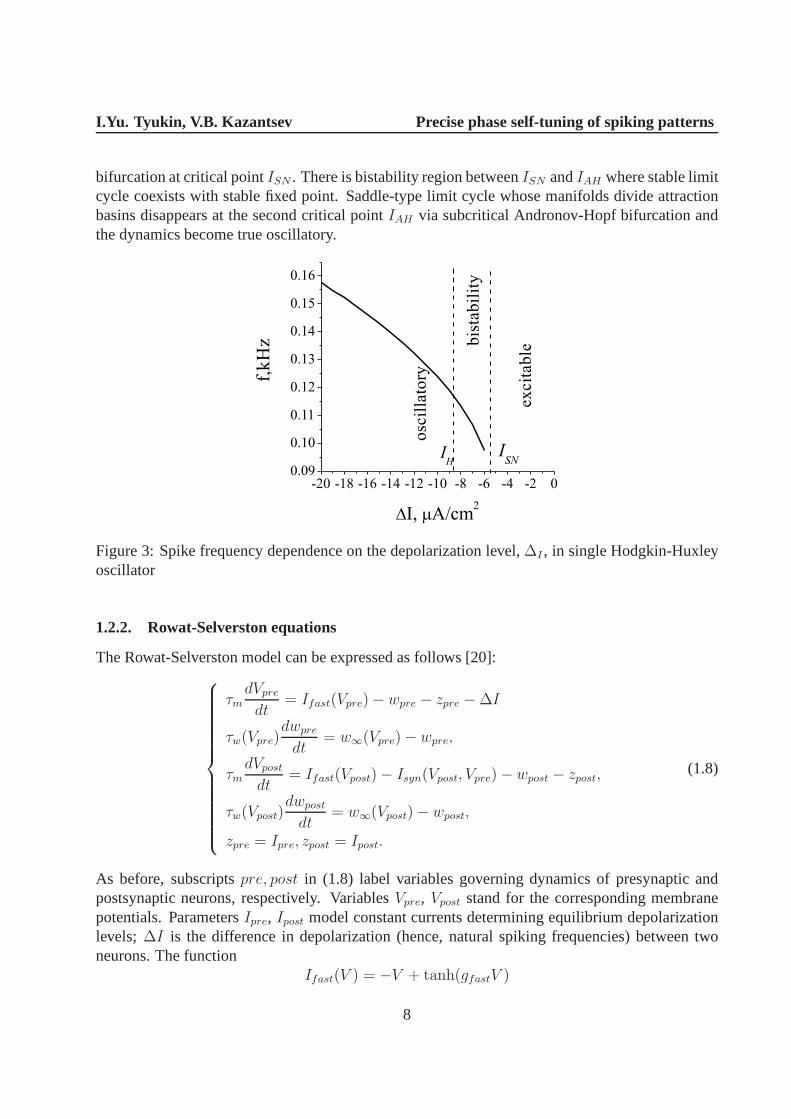
Let us illustrate first the dynamics of uncoupled oscillators, e.g.gsyn = 0. For simplicity, wesetzpre = zpost = 0 and consider the dynamics of the presynaptic neuron depending on∆I playingthe role of an external current controlling the depolarization level. Figure 3 illustrates monotonicdependence of oscillation frequency on∆I. The oscillation appears from saddle-node limit cycle
7
I.Yu. Tyukin, V.B. Kazantsev Precise phase self-tuning of spiking patterns
bifurcation at critical pointISN . There is bistability region betweenISN andIAH where stable limitcycle coexists with stable fixed point. Saddle-type limit cycle whose manifolds divide attractionbasins disappears at the second critical pointIAH via subcritical Andronov-Hopf bifurcation andthe dynamics become true oscillatory.
Figure 3: Spike frequency dependence on the depolarizationlevel,∆I , in single Hodgkin-Huxleyoscillator
1.2.2. Rowat-Selverston equations
The Rowat-Selverston model can be expressed as follows [20]:
τmdVpre
dt= Ifast(Vpre)− wpre − zpre −∆I
τw(Vpre)dwpre
dt= w∞(Vpre)− wpre,
τmdVpost
dt= Ifast(Vpost)− Isyn(Vpost, Vpre)− wpost − zpost,
τw(Vpost)dwpost
dt= w∞(Vpost)− wpost,
zpre = Ipre, zpost = Ipost.
(1.8)
As before, subscriptspre, post in (1.8) label variables governing dynamics of presynapticandpostsynaptic neurons, respectively. VariablesVpre, Vpost stand for the corresponding membranepotentials. ParametersIpre, Ipost model constant currents determining equilibrium depolarizationlevels;∆I is the difference in depolarization (hence, natural spiking frequencies) between twoneurons. The function
Ifast(V ) = −V + tanh(gfastV )
8

I.Yu. Tyukin, V.B. Kazantsev Precise phase self-tuning of spiking patterns
Parameter Values
Ipre, Ipost,∆I 0.5, 0.5, [-1.1÷0.2]
gfast, gslow 2.0, 2.0
τm, τ1, τ2, kτ 0.16, 5.0 , 50.0 , 0.05
Vsyn, Θsyn, ksyn, gsyn 1.0, 0.0, 0.16, [0.0÷1.0]
Table 1: Parameters of model (1.8)
models fast currents across cell membrane, andgfast is the conductance of the fast voltage-dependentinward current, Variableswpost, wpre are the slow recovery variables, andw∞(V ) = gslowV is thevoltage-dependent activation function;gslow is the corresponding conductance. Time scales of thespikes are determined by parameterτm > 0 and the function
τw(V ) = τ2 +τ1 − τ2
1 + exp−V
kτ
.
The functionτw(V ) is the voltage dependent characteristic time of the slow current, andτ1, τ2, kτare parameters. We consider the case whenτ1,2 ≫ τm andτw(V ) ≫ τm, andτ2 > τ1. This ensuresthat duration of individual spikes is small relative to the inter-spike intervals.
Synaptic current variable,Isyn, is defined as in (1.6). The values of all relevant parametersofthe model are provided in Table 1. Whengsyn = 0 pre- and post-synaptic oscillators are uncoupled,both producing sequences of pulses with constant, albeit different, firing rate.
The oscillation in each uncoupled compartment appear through the saddle-node limit cyclebifurcation [6, 21]. In terms of Eqs. (1.8), such bifurcation occurs when parameter∆I reachessome critical value. This mimics depolarization of the membrane by a constant current injection.Dependence of the spiking rates on the depolarization levels is similar to one obtained for theHodkin-Huxley model (Fig. 4). In Fig.4, labelsI1 andI2 mark maximal and minimal values of∆I for which the dynamics of both compartments is oscillatory.If the values of∆I are outsideof this interval then the system is in the excitable mode2. If ∆I is within the interval[I2, I1] thenthe frequency curve,f(∆I), is a strictly monotone and continuous function. Thus in this intervalthere is a one to one correspondence between the depolarization parameter∆I and the spike firing
2It is necessary to mention here that in principle there are very narrow intervals to the left ofI2 and to the right ofof I1 in which unstable limit cycle exists. These are not shown in the figure.
9

I.Yu. Tyukin, V.B. Kazantsev Precise phase self-tuning of spiking patterns
Figure 4: Spike oscillation frequency (e.g. natural frequency) as a function of the level of depolar-ization in single neuron model described by Eqs. (1.8). The values of frequencyf are computedfor the dimensionless model.
rate,f . Note, that in contrast with Hodgkin-Huxley model the interval of bistability is negligiblysmall in the Rowat-Selverston model and can be neglected in further consideration.
2. Analysis
2.1. Relative phase dynamics and stabilizing effect of STDP
For the sake of simplicity in this section we will consider the case when individual spikes aregenerated by (1.8) and, furthermore, will focus on the configuration in which only one of the twocoupled phase oscillators, e.g. postsynaptic, is suppliedwith the STDP-type mechanism. We willalso assume that if the value ofzpost is fixed (within an interval) then both oscillators operate in avicinity of asymptotically stable limit cycles. In addition, we will suppose that the values ofgsynare negligibly small so that we can investigate stabilizingeffects of STDP in the combined systemindependently from effect of phase pulling due to the instantaneous synaptic coupling betweenoscillators [7].
Under the assumptions above, phase of the oscillations inVpre, wpre-system (see e.g. [18]) canbe defined as a functionφpre(Vpre, wpre,∆I) such that
∂φpre
∂Vpre
Vpre +∂φpre
∂wpre
wpre = ω0(Ipre +∆I), (2.1)
whereω0(Ipre + ∆I) is the natural frequency of oscillations. Since the frequency of oscillationsdecreases with∆I (see Fig. 4), the functionω0(·) is strictly monotone and non-increasing. More-over, for a technical reason we will assume that the functionω0(·) is differentiable or that it can beapproximated by a differentiable function in the domain of interest.
10

I.Yu. Tyukin, V.B. Kazantsev Precise phase self-tuning of spiking patterns
Similarly, if the value ofzpost is fixed, phase of the oscillations inVpost, wpost-system can beexpressed as a functionφpost(Vpost, wpost, zpost) such that
∂φpost
∂Vpost
Vpost +∂φpost
∂wpost
wpost = ω0(zpost), (2.2)
Notice that if the value ofzpost is allowed to vary and|zpost| is sufficiently small, thenφpost ≃ω0(zpost) provided that|ω0(zpost)| ≫ |zpost|. The latter inequality reflects that the frequency ofoscillations is much higher than the time constant of the STDP. In what follows we will considerthe case when this asymptotic holds.
Taking (2.1), (2.2) into account we can conclude that dynamics of the relative phase,ϕ, is tosatisfy the following equation
ϕ = ω0(zpost)− ω0(Ipre +∆I).
Suppose that the variableΦ in (1.2) evolves according to the following rule:
Φi =tpost(i)− tpre(i)
Tpre
,
wheretpost(i), tpre(i) are the time instances of postsynaptic and corresponding presynaptic events.Denotingω0(zpost)− ω0(Ipre +∆I) = ω − f(zpost), wheref(·) is a continuous, locally Lipschitz,strictly monotone non-decreasing function, andω ∈ R is the frequency de-tuning parameter, wearrive at the following system of equations:
ϕ = ω − f(zpost)
zpost = αpost(Ipost − zpost) + kpostG(σ(ϕ, t, i))) + λpost,(2.3)
whereσ(ϕ, t, i) = Φi, t ∈ [tpost(i), tpost(i) + Tpost(i)).
With regards to the values ofω, we will assume thatω ∈ range(f). It is also clear thatϕ(tpost(i)) =Φi, i = 1, 2, . . . according to the definition of variableΦi.
Let t ∈ [tpost(i), tpost(i) + Tpost(i)), then the last equation in (2.3) can be explicitly integratedgiving rise to
zpost(t) =e−αpost(t−tpost(i))z(tpost(i)) +kpostαpost
(1− e−αpost(t−tpost(i)))G(σ(ϕ, t, i)))
+
(
λpost
αpost
+ Ipost
)
(1− e−αpost(t−tpost(i)))
(2.4)
Thus taking (2.3) and (2.4) into account and approximating the functionf(·) by a linear one3,
3This is a plausible assumption given that the curve shown in Fig. 4 and depicting dependence of frequency on theexcitation parameter can be approximated by a segment of a line.
11

I.Yu. Tyukin, V.B. Kazantsev Precise phase self-tuning of spiking patterns
f(zpost) = f ∗ + f0zpost, we can now expressϕ(t) for t ∈ [tpost(i), tpost(i) + Tpost(i)) as:
ϕ(t) =ϕ(tpost(i)) + ω(t− tpost(i))− f ∗(t− tpost(i))− f0[ 1
αpost
(1− e−αpost(t−tpost(i)))z(tpost(i))
+
(
kpostαpost
G(σ(ϕ, t, i)) +
(
λpost
αpost
+ Ipost
))(
(t− tpost(i))−1− e−αpost(t−tpost(i))
αpost
)
]
.
Noticing thatϕ(tpost(i) + Tpost(i)) = Φi+1, ϕ(tpost(i)) = Φi, denotingzi = zpost(tpost(i)), zi+1 =zpost(tpost(i) + Tpost(i)), and using the fact thatϕ(t) is continuous int, we arrive at
Φi+1 =Φi + ωTpost(i)− f ∗Tpost(i)− f0[ 1
αpost
(1− e−αpostTpost(i))zi
+
(
kpostαpost
G(Φi) +
(
λpost
αpost
+ Ipost
))(
Tpost(i)−1− e−αpostTpost(i)
αpost
)
]
zi+1 =e−αpostTpost(i)zi +
(
kpostαpost
G(Φi) +
(
λpost
αpost
+ Ipost
))
(1− e−αpostTpost(i))
(2.5)
LetΦ∗, z∗ be an equilibrium of (2.5). Given thatG(·) is differentiable, and neglecting dependenceof Tpost(i) on zpost if zpost is close enough toz∗ , we can linearize the dynamics of (2.5) aboutΦ∗, z∗:
(
Φi+1 − Φ∗
zi+1 − z∗
)
= Ki
(
Φi − Φ∗
zi − z∗
)
, Ki =
(
k11(i) k12(i)k21(i) k22(i)
)
(2.6)
where
k11(i) =1−f0G0kpostαpost
(
Tpost(i)−1− e−αpostTpost(i)
αpost
)
k12(i) =−f0
αpost
(1− e−αpostTpost(i))
k21(i) =G0kpostαpost
(1− e−αpostTpost(i))
k22(i) =e−αpostTpost(i)
G0 =G′(Φ∗, z∗).
(2.7)
DenotingδΦ = Φ∗ − Φc we rewrite (2.6) as(
Φi+1 − Φc
zi+1 − z∗
)
= Ki
(
Φi − Φc
zi − z∗
)
− ui, ui =
(
k11(i)− 1k21(i)
)
δΦ. (2.8)
where, according to the second equation in (2.5) atzi+1 = zi = z∗, the value ofδΦ is
δΦ = G−1
(
−λpost − αpost(Ipost − z∗)
kpost
)
.
12

I.Yu. Tyukin, V.B. Kazantsev Precise phase self-tuning of spiking patterns
Let σ1, σ2 be eigenvalues of the matrix
Ki =
(
k11(i) k12(i)k21(i) k22(i)
)
Then, provided that the fluctuations ofTpost(i) are sufficiently small, condition|σ1| < 1, |σ2| < 1ensures that the fixed pointΦ∗, z∗ is stable in the sense of Lyapunov.
The eigenvalues ofKi can be expressed as
σ1,2 =(k11(i) + k22(i))±
√
(k11(i) + k22(i))2 − 4(k11(i)k22(i)− k12(i)k21(i))
2. (2.9)
According to (2.7), (2.9), checking if|σ1| < 1, |σ2| < 1 holds requires availability of the esti-mates/values off0 andG0. The value off0 can be explicitly inferred from Fig. 4:f0 ≃ 0.025,and the value ofG0 belongs to[0, 2π]. Figure 5 shows plots of|σ1|, |σ2| as functions ofkpost forαpost = 0.01, G0 = 2π, and two different values ofTpost: Tpost = 35 (green curve), andTpost = 50(blue curve). According to the figure, there is a range of values ofkpost for which both|σ1| and|σ2| are less than one, and hence the fixed point is stable.
Figure 5: Stability diagram derived from the local analysisof the fixed points of (2.5). Blue lineshows the values of|σ1|, |σ2| (eigenvalues of the Jacobian of (2.5), see also (2.9)) as functions ofkpost for Tpost = 50. Green line depicts the values of|σ1|, |σ2| for Tpost = 35. Other parametervalues were set as follows:αpost = 0.01, f0 = 0.025, G0 = 2π, gsyn = 0. Blue and green circlesindicate critical values ofk∗
post(Tpost), for Tpost = 50 andTpost = 35 respectively, at which thefixed pointΦ∗, z∗ becomes unstable.
Summarizing the analysis above one can conclude that
• if f0, G0 > 0 then, for a broad range ofTpost, there will always exist values of the STDPparameters,kpost, αpost, such that the fixed point of (2.5) is locally exponentially stable forthese values;
13

I.Yu. Tyukin, V.B. Kazantsev Precise phase self-tuning of spiking patterns
• the values of relative phase mismatches,δΦ, corresponding to the fixed point depends recip-rocally on the value ofkpost; the larger is the absolute value ofkpost, the smaller is the valueof |δΦ|
• however, if the values ofkpost are made large enough, i.e. whenmax|σ1|, |σ2| > 1 (whichis always possible to achieve, see (2.7), (2.9)), the corresponding fixed point becomes unsta-ble.
Remark 1. An alternative strategy for assessing stability of the equilibria of (2.3) can be carriedout without explicit integration of the second equation in (2.3). If kpost ∈ R>0, αpost ∈ R>0 aresufficiently small then solutions of (2.3) can be approximated by that of
ϕ = ω − f(zpost)
zpost = αpost(Ipost − zpost) + kpostG(ϕ− Φc)) + λpost.(2.10)
It is clear that equilibria of (2.10) can be determined from
z∗ = f−1(ω)
Φ∗ ∈ G−1
(
−αpost(Ipost − f−1(ω))− λpost
kpost
)
+ Φc
(2.11)
whereG−1 is, in general, a set-valued function. IfΦ∗ is such that∂G/∂ϕ(Φ∗ − Φc) > 0 then onecan conclude thatΦ∗, z∗ is an asymptotically stable equilibrium of (2.3). The conclusion followsfrom the analysis of the time-derivative of the following Lyapunov candidate:
V (ϕ, zpost) =
∫ zpost
z∗(f(s)− f(z∗))ds+ kpost
∫ ϕ
Φ∗
G(s)−G(Φ∗)ds
followed by invoking the Barbalatt’s lemma for demonstrating asymptotic convergence ofϕ(t) toΦ∗.
In order to proceed with the analysis further a technical result provided in the next paragraphsis required
2.2. Local non-uniform small gain theorem
Consider a system with input,u, and let the evolution of its state,x, be governed by
x = f(x, u(t), t), (2.12)
where the functionf : Rn × R× R → Rn is locally bounded inx, u, bounded int, andu : R →
R is a continuous function. For the sake of notational compactness we denote‖z(τ)‖∞,[a,b] =maxτ∈[a,b] ‖z(τ)‖, wherez is a function defined on[a, b]. LetΩ(t0, t) = Ωx ×Ωu(t0, t), Ωx : x ∈R| ‖x‖ ≤ ∆x, ∆x ∈ R>0, Ωu(t0, t) = u| u : R → R, u ∈ C0, ‖u‖∞,[t0,t] ≤ ∆u, and suppose
14

I.Yu. Tyukin, V.B. Kazantsev Precise phase self-tuning of spiking patterns
that for anyt0 ∈ R, t > t0 and all(x0, u) ∈ Ω(t0, t), the solutions of (2.12) satisfyingx(t0) = x0
are defined, and the following holds
‖x(t0 + T )‖ ≤ β(T )‖x(t0)‖+ c‖u(t)‖∞,[t0,t0+T ] +∆p, ∆p ∈ R≥0, T ∈ [0, t− t0], c ∈ R≥0,
whereβ(T ) is a strictly monotone continuous function:limt→∞ β(t) = 0, β(0) ≥ 1. Let ussuppose that for allt0 inputu in (2.12) is evolving according to
u(t0) ≥ u(t) ≥ u(t0)− (t− t0)γ‖x(t′) +D(t′)‖ε, t
′ ∈ [t0, t], t ≥ t0, γ ∈ R>0, (2.13)
where‖x‖ε stands for‖x‖ − ε if ‖x‖ > ε and0 otherwise, andD : R → R is a bounded function:‖D(t′)‖ ≤ ∆d for all t′. Then the following statement holds for interconnection (2.12), (2.13) (cf.[24], [25])
Theorem 1. Consider interconnection (2.12), (2.13), and let
ε ≥ ∆p
(
1 + β(0)κ
κ− d
)
+∆d.
Suppose that the domain
Ωγ : 0 ≤ γ ≤ β−1
(
d
κ
)−1κ− 1
κ
u(t0)
β(0)(‖x(t0)‖+ c|u(t0)|(1 + κ/(1− d))) + c|u(t0)|(2.14)
is not empty for somed < 1, κ > 1. LetΩ∆ = (x, u)| β(0)‖x‖+ c|u|+∆p ≤ ∆x, |u| ≤ ∆u.Then for all(x0, u(t0)) ∈ Ωγ ∩ Ω∆ the state(x(t), u(t)) of the interconnection is bounded.
Furthermore, if there is a functionw : Rn → R≥0 such that
u(t) ≤ u(t0)− (t− t0)w(x(t′)), t′ ∈ [t0, t], t ≥ t0, (2.15)
then for every divergent and ordered infinite sequenceti, i = 0, 1, . . . , ti < ti+1, the followingholds:
∃ t′i, t′i ∈ [ti, ti+1] : lim
ti→∞w(x(t′i)) = 0. (2.16)
Proof of Theorem 1. Boundedness.Let us introduce a strictly decreasing sequenceσi, i =0, 1, . . . , such thatσ0 = 1, andσi asymptotically converge to zero. Letti, ti, i = 1, . . . be anordered infinite sequence of time instances such that:
u(ti) = σiu(t0).
If the latter assumption does not hold then one can immediately conclude thatu(t) is bounded frombelow by0 for t ≥ t0; it is also bounded from above byu(t0), for t ≥ t0. Henceu(t) is boundedfor all t ≥ t0. Moreover trajectoryx(t) is bounded for allt ≥ t0, and nothing remains to be proven.We wish to show that the amount of time needed to reach the set(x, u)| u = 0 from the giveninitial condition is larger than any positive number, i.e. infinite.
15
I.Yu. Tyukin, V.B. Kazantsev Precise phase self-tuning of spiking patterns
Consider time differencesTi = ti − ti−1. It is clear that:
Ti maxτ∈[ti−1,ti]
‖x(τ) +D(τ)‖ε ≥u(t0)(σi−1 − σi)
γ. (2.17)
Sincemaxτ∈[ti−1,ti] ‖x(τ) +D(τ)‖ε = ‖x(τ) +D(τ)‖∞,[ti−1,ti]− ε if ‖x(τ) +D(τ)‖∞,[ti−1,ti] > ε,andmaxτ∈[ti−1,ti] ‖x(τ) +D(τ)‖ε = 0 overwise, we can see from (2.17) that
Ti ≥
u(t0)(σi−1−σi)γ
1‖x(τ)+D(τ)‖
∞,[ti−1,ti]−ε, ‖x(τ) +D(τ)‖∞,[ti−1,ti] > ε;
∞, ‖x(τ) +D(τ)‖∞,[ti−1,ti] ≤ ε.(2.18)
We will consider the case when‖x(τ) +D(τ)‖∞,[ti−1,ti] − ε > 0 for all i = 1, 2, . . . (sinceu(t) isclearly bounded overwise).
In addition toti we introduce another auxiliary sequenceτi, τi = τ ∗, τ ∗ ∈ R>0, i = 1, . . . .Given that the partial sums
∑
i τi =∑
i τ∗ diverge we can conclude that proving the implication
Ti ≥ τ ∗ ⇒ Ti+1 ≥ τ ∗ ∀ i (2.19)
will automatically assure thatx(t), u(t) are bounded for allt ≥ t0. We prove (2.19) by inductionwrt i.
Let us pickτ ∗ = β−1 (d/κ) , d ∈ (0, 1), (2.20)
and select the value ofγ such that (2.14) holds.Letx(t0), u(t0) be such thatβ(0)‖x(t0)‖+ c|u(t0)|+∆p < ∆x, 0 < u(t0) < ∆0. The function
u(t) is non-increasing over[t0, ti]. This ensures thatu ∈ Ωu(t0, ti), and hencex(ti), u(ti) ∈ Ω∆
for all ti. Suppose thatTj ≥ τ ∗ for 1 ≤ j ≤ i− 1. Therefore
‖x(τ)‖∞,[ti−t,ti]≤ β(0) ‖x(ti−1)‖+ cu(t0)σi−1 ≤ β(0) [β(Ti−1) ‖x(ti−2)‖+ cu(t0)σi−2] + cu(t0)σi−1
≤ β(0)β2(τ ∗) ‖x(ti−3)‖+ P2,
where
P2 = β(0) [β(τ ∗)cσi−3 + cσi−2] u(t0) + cσi−1u(t0) + β(0)[β(τ ∗)∆p +∆p] + ∆p
Repeating this iteration with respect toi leads to
‖x(τ)‖∞,[ti−t,ti]≤ β(0)β3(τ ∗) ‖x(ti−4)‖+ P3
P3 = cu(t0)β(0)[
β2(τ ∗)σi−4 + β(τ ∗)σi−3 + σi−2
]
+ σi−1cu(t0) + ∆pβ(0)[β(τ∗)2 + β(τ ∗) + 1]
+ ∆p = cu(t0)β(0)
[
2∑
j=0
βj(τ ∗)σi−j−2
]
+ cu(t0)σi−1 +∆pβ(0)
[
2∑
j=0
βj(τ ∗)
]
+∆p,
16

I.Yu. Tyukin, V.B. Kazantsev Precise phase self-tuning of spiking patterns
and afteri− 1 steps we obtain
‖x(τ)‖∞,[ti−t,ti]≤ β(0)β(τ ∗)i−1 ‖x(t0)‖+ Pi−1
Pi−1 = cu(t0)β(0)
[
i−2∑
j=0
βj(τ ∗)σi−j−2
]
+ cu(t0)σi−1 +∆pβ(0)
[
i−2∑
j=0
βj(τ ∗)
]
+∆p.(2.21)
Rearranging terms in (2.17) results in
Ti ≥σi−1 − σi
σi−1
u(t0)
γ
1
σ−1i−1(‖x(τ) +D(τ)‖∞,[ti−1,ti]
− ε).
Hence, if we can show that there exist anx0 such that such that for some∆0 ∈ R≥0:
σi−1 − σi
σi−1
u(t0)
τ ∗≥ ∆0 (2.22)
the following holds
γσ−1i−1(‖x(τ) +D(τ)‖∞,[ti−1,ti]
− ε) ≤ γB(x0) ≤ ∆0 ∀ i,
whereB(·) is a function ofx0, then implication (2.19) will obviously follow.Considerσ−1
i−1(‖x(τ) +D(τ)‖∞,[ti−1,ti]− ε), and let
σi =1
κi, κ > 1
According to (2.21) we have:
σ−1i−1(‖x(τ) +D(τ)‖∞,[ti−1,ti]
− ε) ≤ β(0)[
σ−1i−1β(τ
∗)i−1]
‖x(t0)‖+ σ−1i−1Pi−1 + σ−1
i−1∆d
= β(0)(κβ(τ ∗))i−1 ‖x(t0)‖+ κi−1(Pi−1 +∆d)
= β(0)(κβ(τ ∗))i−1 ‖x(t0)‖+ cu(t0)β(0)κ
[
i−2∑
j=0
βj(τ ∗)κj
]
+ cu(t0)+
κi−1
[
∆p
(
β(0)i−2∑
j=0
βj(τ ∗) + 1
)
+∆d − ε
]
.
Hence choosing the value ofτ ∗ as in (2.20)
κβ(τ ∗) = d, d ∈ (0, 1)
lettingε ≥ ∆p
(
1 + β(0) κκ−d
)
+∆d, and noticing that
κi−1
[
∆p
(
β(0)
i−2∑
j=0
βj(τ ∗) + 1
)
+∆d − ε
]
= ki−1
[
∆p
(
β(0)
1− d/k+ 1
)
+∆d − ε
]
,
17

I.Yu. Tyukin, V.B. Kazantsev Precise phase self-tuning of spiking patterns
we can conclude that
σ−1i−1(‖x(τ) +D(τ)‖∞,[ti−1,ti]
− ε) ≤ β(0) ‖x(t0)‖+ cu(t0)
(
1 +β(0)κ
1− d
)
= B(x0).
Solving (2.20), (2.22) for respect to∆0 results in
∆0 =κ− 1
κ
[
β−1
(
d
κ
)]−1
u(t0).
This in turn implies that for all(x(t0), u(t0)) ∈ Ω∆ which, in addition, satisfy:
γ ≤κ− 1
κ
[
β−1
(
d
κ
)]−1u(t0)
β(0) ‖x(t0)‖+ c|u(t0)|(
1 + κβ(0)1−d
)
the following implication must hold:Ti ≥ τ ∗ ⇒ Ti+1 ≥ τ ∗. Therefore, trajectoriesx(t), u(t)passing throughx(t0), u(t0) at t = t0 are bounded in forward time.
Convergence.Let us show that (2.15) implies (2.16). Suppose that this is not the case, andfor an ordered diverging sequenceti there is aδ > 0 such thatw(x(t′)) > δ, ∀ t′ ∈ [ti−1, ti],i = 1, 2, . . . . Hence
u(ti) ≤ u(ti−1)− (ti − ti−1)δ ≤ u(t0)− (t0 − ti−1)δ. (2.23)
According to the first part of the propositionu(ti) is bounded for alli. On the other hand, using(2.23) one can conclude that for any given arbitrarily largeM , there is ann > 0 such thatu(tn) ≤−M . Thus we have reached contradiction which proves (2.16).
2.3. Phase adaptation
So far we have established that STDP mechanisms (1.1), (1.2)may result in the emergence of thestable fixed point of the relative phase dynamics. The relative phase values corresponding to thisfixed point, however, do not coincide with the reference,Φc. Even though there is a room foroptimizing the phase mismatch,δΦ, by increasing the values of STDP gains, discrete nature ofthe regulatory feedback, imposes a limitation on the degreeto which such an optimization can beused without incurring penalties in the form of the loss of stability of the fixed point. Note that,according to (2.11), if parameters of the STDP law are chosensuch thatαpost(f
−1(ω) − Ipost) −λpost(t) = 0 then the relative phase variable,Φ, (in a neighborhood of the locking state) locks tothe the referenceΦc asymptotically. The problem is, however that the value of natural frequenciesmismatch,ω, is unknown a-priori. Thus annihilating the error by choosing the values ofαpost, Ipost(or αpre, Ipre for the presynaptic feedback) is not a viable option. This motivates introduction ofan extra dynamical process in the system that is capable of producing such an adjustment.
An important consequence of the stability analysis above, specifically (2.3) – (2.8), is that ifλpost is allowed to vary then, subject to the choice ofkpost, αpost, the dynamics of (1.8) in which
18

I.Yu. Tyukin, V.B. Kazantsev Precise phase self-tuning of spiking patterns
zpost evolves in accordance with (1.2) locally satisfies the following constraint:∥
∥
∥
∥
ϕ(t)− Φc
zpost(t)− z∗
∥
∥
∥
∥
≤ β(t− t0)
∥
∥
∥
∥
ϕ(t0)− Φc
zpost(t0)− z∗
∥
∥
∥
∥
+ c · maxt∈[t0,t]
‖λ∗ − λpost(t)‖ , t ≥ t0
λ∗ = −αpost(Ipost − f−1(ω)),
(2.24)
whereβ(·) is a strictly monotone, positive, and non-increasing function vanishing asymptoticallyat infinity, andc is a non-negative constant.
As before we will suppose that only one oscillator (postsynaptic) is equipped with the STDPmechanism, i.e. onlyλpost is adapting. Consider system (2.3) in which the functionλpost(t) evolvesaccording to the following simple rule:
λpost(t0) +Γ
∫ t
t0
|σ(ϕ, τ, i)−Φc|dt ≤ λpost(t) ≤ λpost(t0) + γ
∫ t
t0
|σ(ϕ, τ, i)−Φc|dt, Γ, γ ∈ R>0,
(2.25)whereσ(ϕ, t, i) = Φi for all t ∈ [tpost(i), tpost(i) + Tpost(i)), Tpost(i) > 0, and|λ∗ − λpost(t0)| ≤Mλ. The value ofMλ is supposed to be small enough so that there is a neighborhoodof Φc:|ϕ− Φc| ≤ MΦ such that (2.24) holds for all
|ϕ(t)− Φc| ≤ MΦ, |λ∗ − λpost(t)| ≤ Mλ. (2.26)
According to Theorem 1, if at any givent0 variablesϕ(t0), λpost(t0) of the combined system(2.24), (2.25) satisfy
|ϕ(t0)− Φc| ≤ MΦ, 0 ≤ λ∗ − λpost(t0) ≤ Mλ
then picking
0 ≤ γ ≤ β−1
(
d
κ
)−1κ− 1
κ
Mλ
β(0)(MΦ + c|u|(1 + κ/(1− d))) + cMλ
(2.27)
ensures thatϕ(t) converges toΦc asymptotically.Consider a modified version of (2.25):
λpost(t) = λmin +λmax − λmin
2
(
1− sin
(
2
λmax − λmin
(
λ0 + γ
∫ t
t0
|σ(ϕ, τ, i)− Φc|dτ
)))
,
(2.28)where the value ofγ is chosen according to (2.27), andλ∗ ∈ [λmin, λmax]. Suppose that for anycontinuousλpost(t): λmin ≤ λpost(t) ≤ λmax
1) solutions of (2.3) are defined;
2) for eachλpost fixed,λpost ∈ [λmin, λmax], there is a unique attractor, which is locally expo-nentially stable;
3) there is a neighborhood ofΦc : |ϕ− Φc| < MΦ such that (2.24) holds.
19

I.Yu. Tyukin, V.B. Kazantsev Precise phase self-tuning of spiking patterns
It is therefore clear that one can pickγ so small that solutions of the combined system (2.3), (2.28)will eventually converge into the domain specified by (2.26). In this domain the functionλpost
defined in (2.28) will satisfy (2.25), albeit possibly with different constantsγ,Γ. Hence, Theorem1 applies, and thus one can pickγ > 0 sufficiently small so thatlimt→∞, i→∞ σ(ϕ, t, i) = Φc. This,in turn implies thatϕ(t) → Φc at t → ∞.
This adaptation mechanism described above is in essence a slow fluctuation of the excitationthresholds. The frequency of these fluctuations increases if absolute values of relative phase are faraway from the desired ones. The frequency slows down when relative phase approaches its desiredvalue, i.e. the referenceΦc.
3. Numerical study of the relative phase dynamics in coupledneural oscillators with STDP-regulated parameters
So far we have established analytically that phase-lockingof the relative phase dynamics may occurin a system of generic neural oscillators equipped with an STDP mechanism affecting parametersregulating natural frequencies of oscillations in the system. We have also shown that without anadaptation mechanisms adjusting parameters of the STDP law(or, alternatively, parameters of theoscillators) precise phase locking to a given relative phase value may not be possible to achieve.However, if an adaptation mechanism is added (e.g. (2.28)) then the values of relative phase couldbe stirred to small neighborhoods of the reference.
These results, however, are local and their validity is largely confined to the domain in whichapproximation (2.1) holds. Second, as is often the case in the models of considered type, variableszpre, zpost could be viewed as bifurcation parameters of the model, and as such they are likely to af-fect dynamics of the interconnection beyond cases capturedin the local analysis above. Therefore,in order to ensure that our earlier conclusions retain plausibility, further and extensive numericalstudies are required. These will be presented in the next paragraphs.
3.1. Spiking phase map
In order to characterize and analyze post- to presynaptic timing in (1.8), including cases whenzpreandzpost are varying with time, we introducespiking phase map[14]. The map itself is constructedas follows. First, we define the relative spiking phase,Φ, as:
Φ =tpost − tpre
Tpre
, . . . 0 < Φ < 1, (3.1)
wheretpre is the time corresponding to occurrence of a presynaptic spike, andtpost is the timeof the first postsynaptic spike generated in response to the presynaptic one;Tpre is the period ofoscillations in the presynaptic neuron. VariableΦ, therefore, may be viewed as a sample of relativephase of the oscillators that is measured at the moments of time when the post-synaptic oscillatorfires. Second, having defined a sequence ofΦ over time, we determine thespiking phase mapas
20

I.Yu. Tyukin, V.B. Kazantsev Precise phase self-tuning of spiking patterns
follows:T : Φi → Φi+1, i = 1, 2, . . . ,
Φi =tpost(i)− tpre(i)
Tpre,
(3.2)
wherei is the index of transmitted spikes in the sequence. It was shown in [14] that in the case of
Figure 6: PRC curves for different coupling strengths,∆I = −0.05. A: gsyn = 0. Relative phaseshift is monotonically increasing as it is shown by arrows. The increase is linearly proportionalto the frequency mismatch,∆I. B: PRC for small value of the synaptic coupling,gsyn = 0.008.Monotonically increasing phase is pulled towards the abscissa in the vicinity of the origin. C:Synchronization forgsyn = 0.04. Stable fixed point emerging from the tangent (+1) bifurcationdefines the value of the phase locked with a small synaptic transmission delay. D: Synchronizationfor the increased coupling strength,gsyn = 0.1. The fixed point is close to zero.
constantzpre, zpost transformation (3.2) may be modeled by a one-dimensional point map,Φi+1 =T (Φi), whereT is a piece-wise continuous function on the interval0 < Φ ≤ 1. Stable fixed pointsof this map correspond to the spike synchronization mode1 : 1. Spiking phase in this mode islocked to the value of the fixed point. Note, that thespiking phase mapcan be also viewed as a
21

I.Yu. Tyukin, V.B. Kazantsev Precise phase self-tuning of spiking patterns
discrete version of thepulse coupled equations. These are typically used in the literature on theanalysis of weakly coupled neuronal oscillators for describing dynamics of relative phases in thesystem. The functionT (Φ) in this context is often referred to as thephase response curve(PRC).The advantage of using discrete spiking phase map instead ofits continuous-time counterpart isthat the discrete map, (3.2), is defined for any values of coupling strengths, provided that bothsystems oscillate.
Figure 6 shows typical shapes of the PRCs for (1.8). In the absence of coupling relative phaseshifts increase in a monotone fashion (Fig. 6A). Adding a small coupling alternates the dynamicsand, respectively, PRCs. Figure 6 B shows the spiking phase map near the tangent or+1 bifurca-tion. There appears to be a region (a ghost) in the figure whichis pulling and trapping, for quitea long period of time, the values ofΦi. The effect is illustrated in more detail in Fig. 7A. Notice
Figure 7: Oscillations in synaptically coupled oscillators Eqs. (1.8). Upper panel shows the mem-brane potentials in presynaptic (dashed curve) and in postsynaptic neurons (solid curve), respec-tively. The lower panel shows time evolution of the relativespiking phase. A: Phase pulling effect.Long lasting quasi-synchronous signals are alternating with phase reset intervals. Parameter val-ues: gsyn = 0.008,∆I = −0.05. B: Synchronization and phase locking due to the excitatorysynaptic coupling. Parameter values:gsyn = 0.1,∆I = −0.05.
that the system’s state may remain in a neighborhood of the synchronous mode for a rather longtime. In the phase space of Eqs. (1.8) this corresponds to solutions near periodic or quasi-periodicorbits on the invariant torus. Further increase ofgsyn leads to appearance of a stable fixed point.The fixed point corresponds to nearly synchronous firing (i.e. with almost zero phase lags) of preand post- synaptic oscillators (Fig. 6C,D). An example of such a solution of (1.8) is shown in Fig.7B.
22

I.Yu. Tyukin, V.B. Kazantsev Precise phase self-tuning of spiking patterns
3.2. STDP with postsynaptic feedback
First, we consider the postsynaptic STDP feedback – the one in which timing of pre- and post-synaptic events changes excitability of the postsynaptic neuron (Fig. 2A). In this case dynamics ofthe presynaptic neuron is not affected. Hence it is plausible to assume that the presynaptic neurongenerates a sequence of spikes with a fixed, albeit unknown, frequency.
Let us investigate dynamics of relative phase for this system. As before, we approach the taskby constructing and analyzing the corresponding spiking phase map. Given that the value ofTpre
is constant, the map is described as follows:
Tpost :
Φi → Φi+1,zpost(ti) → zpost(ti+1)
i = 1, 2, . . . . (3.3)
Yet, for the sake of convenience of illustration we will onlypresent its one-dimensional projectionson the relative phase coordinate,Φ.
Figure 8 illustrates spiking phase map for postsynaptic STDP driven by the pair of Hodgkin-Huxley neurons. (1.5). When the gain,kpost, increases the map undergoes through two majorbifurcations. These bifurcations delimit the boundaries of STDP driven synchronization. Forlower values ofkpost > 0 saddle-node bifurcation takes place (from Fig. 8 A to B) and stable fixedpoint appears. It exists until period-doubling bifurcation for relatively highkpost (Fig. 8 D).
Similar scenario can be found for the reduced model (1.8). Weanalyze in details the period-doubling transition (Fig. 9). The STDP feedback stabilizesrelative phase in a neighborhood ofthe reference value. Corresponding PRCs are shown in Fig. 9A. The figure suggests presence of astable fixed point,Φ∗. If one increases the value ofkpost the fixed pointΦ∗ looses stability throughthe period doubling bifurcation. To the right of this critical point behavior of the system resemblesa route to chaos through the period doubling cascade (Fig. 9B) [6]. In contrast to the previouslyconsidered configuration (presynaptic STDP feedback), in this case relative phase remains in avicinity of the fixed point even if the fixed point itself becomes unstable. The values of relativephase, however, appear to be attracting to a stable2m-periodic orbit or to a set with a structure ofa chaotic attractor. Corresponding plots of the evolution of Φ andzpost are shown in Fig. 10A,B.Further increments ofkpost lead to a catastrophe of the attractor. The catastrophe occurs becausethe values ofzpost become so large that oscillations in the postsynaptic neuron disappear (see Fig.4).
The fact that a set on which the values ofΦ project resembles an object looking strikingly simi-lar to a chaotic attractor suggests a rather unexpected function of the STDP mechanism consideredhere. The function is that such STDP-induced dynamics may offer a natural facility for encodingof information in the system. Indeed, if this set is a chaoticattractor then it comprises of infinitenumber of orbits with varying periods. Thus, in principle, arich set of spiking sequences can beactivated in such a system if an appropriate stimulus arrives.
Bifurcation diagrams characterizing dynamics of the system are shown in Fig. 11. When thevalues ofkpost are relatively small no locking occurs. If we increase the value of kpost (up tothe first critical point), relative phase will eventually lock to a value corresponding to nearly in-phase oscillations. Again, the phenomenon is very similar to the case of presynaptic configuration:
23

I.Yu. Tyukin, V.B. Kazantsev Precise phase self-tuning of spiking patterns
Figure 8: Postsynaptic STDP driven PRC curves for differentfeedback gains,∆I =−1µA/cm2, gsyn = 0,Φc = 0.6. A: kpost = 0. Relative phase shift is monotonically increas-ing proportionally to the frequency mismatch,∆I. B: PRC for small value of the feedback gain,kpost = 0.1. The stable fixed point corresponds to synchronization withphase shift close to thephaseΦC . C: PRC forkpost = 0.3. D: PRC forkpost = 0.5. The fixed point loses stability throughthe period-doubling bifurcation.
STDP facilitates in-phase oscillations even if the synaptic connection is relatively week. Ifkpostis increased even further (until the second critical value)relative phase locks near the referenceΦc. Further increments ofkpost result in gradual improvements of accuracy until, however,kpostarrives at the third critical value. At this point the perioddoubling bifurcation occurs in the spikingphase map (3.3). Increasing the value ofkpost beyond this critical point gives rise to the bifurcationcascade. The latter, in turn, leads to emergence of chaotic-looking dynamics [6, 21] of the relativephase (Fig. 9B, Fig. 10B). This state, however, is also limited in terms of the range of admissiblevalues ofkpost. If kpost becomes too large, i.e. it exceeds the forth critical value,oscillations in thepostsynaptic neuron disappear (Fig. 11A).
24

I.Yu. Tyukin, V.B. Kazantsev Precise phase self-tuning of spiking patterns
Figure 9: The PRCs for the one-dimensional approximation ofthe spiking phase map (3.3). A:Appearance of the stable fixed point forkpost = 0.002 indicating phase locking mode in the signaltransmission with reference phaseΦc = 0.6. Grey curve shows the PRC without control. B: ThePRC for large control strength,kpost = 0.0063, indicating the appearance of chaotic attractor. Thedots show the trajectory of the two-dimensional map (3.3). Parameter values:αpost = 0.01,∆I =−0.05, gsyn = 0.
3.3. STDP with presynaptic feedback
Consider system (1.8), (1.1), and (1.4). Dynamics of this configuration forkpre > 0 is illustratedin Figure 12A. One can observe that, after a relatively shorttransient behavior, the relative phase,Φ, locks near the reference value,Φc. According to the figure, the transient looks like dampedoscillation relaxing asymptotically to a stable fixed point. When the relative phase locks presynap-tic neuron changes its depolarization level (Fig. 12A-C, lower panel). Notice that locking occursfor both zero and nonzero synaptic coupling. Figure 12B illustrates dynamics of the system inthe phase pulling mode (see Fig. 6B). If the coupling betweencells is made relatively strong thenpresynaptic STDP feedback may destroy the in-phase synchronization mode and switch the systeminto the phase-locked mode determined by the value of reference phase (Fig. 12C).
The values at which relative phase locks are determined by the values of the control variable,zpre, at the fixed point. The values ofzpre and relative phase at the fixed point (denoted byz∗pre andΦ∗ respectively) can be determined from (1.1):
−αpre(Ipre − z∗pre)− kpreG(Φ∗) = 0. (3.4)
Hence, according to (1.4) the value of phase locking mismatch, δΦ, can be estimated as follows
δΦ = Φ∗ − Φc = −1
2πarcsin
αpre(Ipre − z∗pre)
kpre. (3.5)
The larger is the value ofkpre, the higher is the precision of phase locking. Notice, however, that ifthe feedback gain,kpre, exceeds a critical threshold, the STDP phase locking regulatory mechanism
25

I.Yu. Tyukin, V.B. Kazantsev Precise phase self-tuning of spiking patterns
Figure 10: Evolution of spiking phase and control variablezpost for postsynaptic control. A: Phaselocking. Parameter values:αpost = 0.01,∆I = −0.05, gsyn = 0, kpost = 0.002. B: Chaotic oscil-lation of the spiking phase near the reference phase. The strength of the feedback is changed in twosteps marked by the arrows. Parameter values:αpost = 0.01,∆I = −0.05, gsyn = 0.00, kpost =0.002, 0.0063.
described above may fail. Loss of stability of the fixed pointis a possible explanation for thisobservation. For extremely large values ofkpre one can observe an “overregulation” catastrophe(Figure 12D). In short, STDP suppresses presynaptic neuronso hard that the neuron is eventuallydriven into excitable mode. This is shown in the upper panel of Fig. 12D. The value ofzpreexceeds the critical value,I1 (see Fig. 4), and the presynaptic neuron becomes inhibited:no spikesare evoked.
26

I.Yu. Tyukin, V.B. Kazantsev Precise phase self-tuning of spiking patterns
Figure 11: Bifurcation and stability diagrams for the case of postsynaptic control.Left panel:phase control bifurcation diagram. Values of the outcome phaseΦ driven by Eqs. (1.2) versusfeedback strength,kpost. Parameter values:αpost = 0.01,∆I = −0.05, gsyn = 0.008,Φc = 0.6.Right panel:A copy of Fig. 5 showing analytically derived stability diagram for this configuration.Notice that stability diagram in the right panel (derived analytically) is largely consistent withthe bifurcation diagram in the left panel (obtained by meansof numerical simulations). Slightinconsistencies are evident in the area wherekpost are small. These inconsistencies are due to that1) our analytical derivations ignore the influence of synaptic coupling,Isyn, and that 2) the fixedpoint may disappear whenkpost small.
In order see the range of parameters for which presynaptic STDP can be considered as a viablephase locking mechanism we calculated numerically dependence ofΦ∗ on kpre (Fig. 13). Whenkpre is small the relative phaseΦ is not settling to a particular constant value; it “scans” throughthe whole interval of admissible values,[0, 1). If kpre is increased beyond a threshold value therelative phase locks. Increasing the value ofkpre further results in locking of relative phase in aneighborhood of the reference,Φc, as predicted by (3.5).
With regards to the influence of STDP model (1.1) on behavior of the coupled system an in-teresting phenomenon can be observed: in-phase oscillations become apparently stable at somecritical value ofkpre (lower left corner of the plot). In other words, presynapticSTDP facilitatesexisting synaptic connections by providing synaptic efficacy equivalent to stronger synaptic cou-pling (transition from Fig. 6B to Fig. 6C). For larger valuesof kpre relative phaseΦ jumps to aneighborhood of the reference phaseΦc. According to the figure, increments ofkpre (in a relativelybroad interval) result in improvements of the phase lockingaccuracy: relative phaseΦ approachesΦc with the growth ofkpre. There is, however, a critical value ofkpre = k∗ at which the fixed pointbecomes neutrally stable. Further increments ofkpre result in destabilization of the fixed point.
In order to assess stability of the relative phase dynamics we invoke the idea of spiking phase
27

I.Yu. Tyukin, V.B. Kazantsev Precise phase self-tuning of spiking patterns
Figure 12: Dynamics of two neuronal oscillators with presynaptic control. Upper and the lowerpanels show the evolution of the relative phase shift (in A-C) and control variable,zpre, re-spectively. A: No synaptic coupling. Parameter values:αpre = 0.01, kpre = 0.002,∆I =−0.05, gsyn = 0,Φc = 0.6. B: Phase pulling mode. Parameter values:αpre = 0.01, kpre =0.002,∆I = −0.05, gsyn = 0.008,Φc = 0.6. C: Switching the phase locking mode from theunsupervised mode (defined by the synaptic coupling) to the one enslaved by the reference phase.Parameter values:αpre = 0.01, kpre = 0.002,∆I = −0.05, gsyn = 0.01,Φc = 0.6. D: Failure ofthe phase control due to overregulation effect. The upper panel shows membrane potentials in twoneurons. Parameter values:αpre = 0.01, kpre = 0.003,∆I = −0.05, gsyn = 0.008,Φc = 0.6.
maps. Here the one-dimensional spiking phase map is extended as follows:
Tpre :
Φi → Φi+1,zpre(ti) → zpre(ti+1),Tpre(i) → Tpre(i+ 1).
i = 1, 2, . . . . (3.6)
VariableTpre(i) is the period of presynaptic spikes; it is now time-varying due to the STDP feed-back. Since there is a functional dependence betweenΦi andTpre(i), map (3.6) can be approxi-mated by a two-dimensional one describing dynamics of the variables(Φi(Tpre(i)), zpre(ti)).
Investigating dynamics of (1.8), (1.1), (1.4) numericallywe have found that the critical gaink∗
corresponds to the neutral stability ofΦ∗ with zero real part of its complex conjugate multipliers.Therefore, Neimark-Saccer bifurcation takes place atkpre = k∗ [6]. Figure 14 shows trajectoriesof the spiking phase map in the vicinity ofk∗. One can see from this figure that ifkpre < k∗ thenvariables(Φi, zpre(ti)) travel towards the stable fixed point (see Figs. 14 A and C). If, however,
28

I.Yu. Tyukin, V.B. Kazantsev Precise phase self-tuning of spiking patterns
Figure 13: Phase control bifurcation diagram. Values of theoutcome phaseΦ driven by Eqs. (1.1)versus feedback strength,kpre. Parameter values:αpre = 0.01,∆I = −0.05, gsyn = 0.008,Φc =0.6.
kpre > k∗ then (Φi, zpre(ti)) move in the opposite direction (see Figs. 14 B and D), and thefixed point appears to be unstable. This behavior indicates that the bifurcation is subcritical (withpositive first Lyapunov coefficient). Thus, forkpre > k∗ relative phaseΦ oscillates with a growingamplitude (Fig. 14 D). One can also observe that forkpre > k∗, which are some distance apartfrom k∗, variablezpre (after a short transient) leaves the domain corresponding to the oscillatorymode (Fig. 4). This, in turn suppresses all oscillations in the presynaptic neuron.
In the bifurcation diagram in Fig. 13 a “cloud” of points emerges whenkpre approaches thecritical pointk∗ from the left. The size of this cloud grows withkpre in a seemingly continuous way.This contrasts with our earlier remark about that the bifurcation is subcritical. Notice, however,that if kpre approachesk∗ from the left, real parts of the linearized map’s eigenvalues are becomingnegligibly small, and also the convergence rate to the fixed point is asymptotically decreasing tozero. Since numerical simulations were run over given and finite interval of time, the amplitude ofthis cloud, i.e. deviations ofΦ from the fixed point at the end of the simulation, depends explicitlyon the convergence rate of the map. The smaller is the convergence rate the higher are the chancesthat deviations ofΦ fromΦc are larger at the end of the simulation. This is exactly what we observein the figure.
29

I.Yu. Tyukin, V.B. Kazantsev Precise phase self-tuning of spiking patterns
Figure 14: The dynamics of map (3.6) in the vicinity of the Neimark-Saccer bifurcation point,kpre = k∗. A and C. Phase plane dynamics and the oscillation profile near stable fixed point forkpre = 0.0054. B and D. Phase plane dynamics and the oscillation profile near unstable fixed pointfor kpre = 0.0057. Parameter values:αpre = 0.01,∆I = −0.05, gsyn = 0.008,Φc = 0.6.
3.4. Adaptive phase-locking STDP
Let us finally investigate performance of the proposed spike-timing dependent adaptation law ofthe baseline variablesλpost (2.28):
λpost = λmin +λmax − λmin
2(1− sin(ζ))
ζ = γ|Φ(ti)− Φc|, γ ∈ R>0, λmax > λmin, λmax, λmin ∈ R,
According to Theorem 1 (see also [24, 25]) such adaptation scheme ensures thatlimi→∞Φi −Φc = 0 provided that the value ofγ is sufficiently small andλmin < minω αpost(z
∗post(ω)− Ipost),
λmax > maxω αpost(z∗post(ω) − Ipost). A very similar adaptation mechanism can be derived for
λpre as well by replacing subscriptspost with pre in the above. Dynamics of adaptive phase-locking STDP in (1.8) with variablezpost evolving according to (1.2) is illustrated in Fig. 15. Thefigure confirms that when extracellular adaptation feedbackis activated the error of phase lockingis slowly vanishing with time.
30

I.Yu. Tyukin, V.B. Kazantsev Precise phase self-tuning of spiking patterns
Figure 15: Adaptive compensation of phase locking errors via extracellular adaptation feedback.Illustration for the case of presynaptic control (1.1). Parameter values:αpre = 0.01,∆I =−0.05, gsyn = 0,Φc = 0.1, kpre = 0.0005, γ = 0.001.
3.5. Difference between Hodgkin-Huxley and Rowat-Selerston models. Ef-fect of bistability
Dynamics of the system in which individual oscillators are described by Hodgkin-Huxley equa-tions remains qualitatively identical to the case of the Rowat-Selverston model (reduced model) ifboth oscillators operate in the oscillatory mode. The qualitative picture, however, changes whenindividual neurons (1.5) are no longer in the oscillatory regime but are functioning in the bistablemode in a vicinity of the saddle-node bifurcation point (Fig. 3). For the chosen set of model pa-rameters, the interval of values of∆I corresponding to the bistable mode in the Rowart-Selverstonmodel is very narrow, and presence of such bistability doesn’t appear to show significant influenceon the dynamics of relative phase in the coupled system. Withregards to the Hodgkin-Huxleyequations, the interval of∆I for which the model is bistable is substantially broader. Inthis casethe inter-play between direct excitatory synaptic coupling and STDP driven depolarization mech-anism can generate trajectories that are persistently “switching” between the limit cycle attractorand the fixed point (neuron resting potential). When the STDPmechanism is activated the spikingphase evolves along the corresponding PRC. As we have illustrated for the case of postsynapticSTDP (see, for example, Fig. 8) it may eventually reach the area (the gap in the figure) where themap itself is undefined. When this occurs the postsynaptic neuron becomes inhibited and its statebegins to relax to the resting potential. Yet, due to the excitatory synaptic coupling, the state maybe moved back to the domain corresponding to the oscillatorymode of the model. In this domainthe system dynamics is again determined by the spiking phasemap. Evidence and examples ofsuch persistent transitions are shown in Fig. 16.
31

I.Yu. Tyukin, V.B. Kazantsev Precise phase self-tuning of spiking patterns
Figure 16: Interplay between direct synaptic coupling and postsynaptic STDP feedback inHodgkin-Huxley neurons (1.5). A. Spiking phase map for the oscillatory mode defined in a cer-tain interval of phase values. B. Trajectories ofVpre, in the presynaptic neuron (dashed curve),andVpost, postsynaptic response (solid curve), as functions oft. Time evolution of the oscillatoryphase on modulus 1. Parameter values:∆I = −1µA/cm2, gsyn = 0.18mS/cm2, kpre = 0, kpost =0.5,Φc = 0.6.
4. Conclusion
In this work we investigated viability of an STDP mechanism affecting neuronal excitability forthe purposes of generating spiking patterns in a pair of coupled oscillators with broadly arbi-trary phase lags between presynaptic and postsynaptic spikes. Theoretical analysis performedunder the assumption that both coupled unites operate in theoscillatory mode predicted limita-tions (with regards to achievable phase lags of spiking) of non-adaptive couplings in the case ofnon-identical systems with different natural frequenciesof oscillation. We have shown, however,that precise timing of signals in the system can still be achieved by means of a slow-varying spike-timing dependent self-tuning of the excitation parametersof the model. These predictions areconfirmed in extensive numerical studies of the system when both oscillators are described eitherby biologically-plausible Hodgkin-Huxley equations or bytheir Rowat-Selverston reduction.
In addition to confirming plausibility of our theoretical findings, numerical analysis revealsrather complicated underlining dynamics of the coupled system. The range of observed phenomenafor the pair of coupled neurons includes: overregulation catastrophe, route to chaos and substantialsensitivity to initial data and parameters when individualoscillators operate in the bistable mode.Observed variability of dynamical modes in such a simple system motivates further investigationin the subject which we hope to perform in future.
With respect to biological realism, our model is based on empirical observations that neuronalexcitability may depend on spike-timing [22]; it is purely phenomenological and is, perhaps, toosimple to be associated with a specific mechanism. It is therefore difficult to suggest a single exper-iment that would allow to validate the model reliably. Nevertheless, we believe that even withoutfirm empirical justification the results can be used for enhancing of phase-locking of spikes in ex-ternally controlled neuronal cultures and animats. We would also like to notice that the resultingfeedback circuits are quite similar by design to phase locked loop (PLL) control systems whichare widely used in communication and engineering. This makes proposed regulatory STDP mech-
32

I.Yu. Tyukin, V.B. Kazantsev Precise phase self-tuning of spiking patterns
anisms readily implementable in artificial networks of electronic or cultured neurons for imitationmodeling and design of neuromorphic and brain inspired information processing systems.
5. Acknowledgment
This research was supported in part by the Federal Program “Scientific and Scientific-educationalbrainpower of innovative Russia” for 2009-2013, by RussianFoundation for Basic Research (grant11-04-12144) and MCB Program of Russian Academy of Science.
References
[1] W.C. Abraham. Metaplasticity: tuning synapses and networks for plasticity.Nature ReviewsNeuroscience, 9:387–399, 2008.
[2] T. Bem and J. Rinzel. Short duty cycle destabilizes a half-center oscillator, but gap junctionscan restabilize the anti-phase pattern.Journal of Neurophysiology, 91:693–703, 2004.
[3] M.A. Diana and P. Bregestovski. Calcium and endocannabinoids in the modulation of in-hibitory synaptic transmission.Cell Calcium, 37(5):497–505, 2005.
[4] A. Dityatev and D.A. Rusakov. Molecular signals of plasticity at the tetrapartite synapse.Current Opinion in Neurbiology, 21(2):353–359, 2011.
[5] W. Gerstner, R. Kempter, J.L. van Hemmen, and H. Wagner. Aneuronal learning rule forsub-millisecond temporal coding.Nature, 386:76–78, 1996.
[6] J. Guckenheimer and P. Holmes.Nonlinear oscillations, dynamical systems, and bifurcationsof vector fields. Springer-Verlag, 1986.
[7] F.C. Hoppensteadt and E.M. Izhikevich.Weakly connected neural networks. Springer-Verlag,1997.
[8] Y. Ikegaya, G. Aaron, R. Cossart, D. Aronov, I. Lampl, D. Ferster, and R. Yuste. Synfirechains and cortical songs: Temporal modules of cortical activity. Science, 304:559–564,2004.
[9] E.M. Izhikevich. Polychronization: Computation with spikes.Neural Computation, 18:245–282, 2006.
[10] E.M. Izhikevich.Dynamical systems in neuroscience. The geometry of excitability and burst-ing. MIT Press, 2007.
[11] E.M. Izhikevich. Solving the distal reward problem through linkage of STDP and dopaminesignaling.Cerebral Cortex, 17:2443–2452, 2007.
33

I.Yu. Tyukin, V.B. Kazantsev Precise phase self-tuning of spiking patterns
[12] C. Kayser, M.A. Montemurro, N.K. Logothetis, and S. Panzeri. Spike-phase coding boostsand stabilizes information carried by spatial and temporalspike patterns.Neuron, 61(4):597–608, 2009.
[13] V. Kazantsev and I. Tyukin. Adaptive and phase selective spike timing dependent plasticityin synaptically coupled neuronal oscillators.PLOS ONE, 7(3):e30411, 2012.
[14] V.B. Kazantsev, V.I. Nekorkin, S. Binczak, S. Jacquir,and J.M. Bilbault. Spiking dynamicsof interacting oscillatory neurons.Chaos, 15:023103, 2005.
[15] H.J. Koester and B. Sakmann. Calcium dynamics in singlespines during coincident pre-and postsynaptic activity depend on relative timing of back-propagating action potentials andsubthreshold excitatory postsynaptic potentials.Proc Natl Acad Sci USA, 95:9596–9601,1998.
[16] F. Lanore, N. Rebola, and M. Carta. Spike-timing-dependent plasticity induces presynap-tic changes at immature hippocampal mossy fiber synapses.The Journal of Neuroscience,29(26):8299–8301, 2009.
[17] T. Ohno-Shosakua, Y. Hashimotodania, T. Maejima, and M. Kano. Calcium signaling andsynaptic modulation: Regulation of endocannabinoid-mediated synaptic modulation by cal-cium. Cell Calcium, 38(3–4):369–374, 2005.
[18] A. Pikovsky, M. Rosenblum, and J. Kurths.Synchronization: a unified concept in nonlinearsciences. Cambridge University Press, 2001.
[19] J.D. Rolston and S.M. Wagenaar, D.A.and Potter. Precisely timed spatiotemporal patterns ofneural activity in dissociated cortical cultures.Neuroscience, 148:294–303, 2007.
[20] P.F. Rowat and A.I. Selverston. Modeling the gastric mill central pattern generator with arelaxation-oscillator network.Journal of Neurophysiology, 70(3):1030–1053, 1993.
[21] L.P. Shilnikov, A.L. Shilnikov, D.V. Turaev, and L.O. Chua.Methods of qualitative theory innonlinear dynamics. World Scientific, 2001.
[22] P.J. Sjostrom, E.A. Rancz, A. Roth, and M. Hausser. Dendritic excitability and synapticplasticity.Physiological Reviews, 88:769–840, 2008.
[23] S. Song, K.D. Miller, and L.F. Abbott. Competitive Hebbian learning through spike-timing-dependent synaptic plasticity.Nature Neuroscience, 3:919–926, 2000.
[24] I. Tyukin. Adaptation in dynamical systems. Cambridge University Press, 2011.
[25] I. Tyukin, E. Steur, H. Neijmeijer, and C. van Leeuwen. Small-gain theorems for systemswith unstable invariant sets.SIAM Journal on Control and Optimization, 47(2):849–882,2008.
34

I.Yu. Tyukin, V.B. Kazantsev Precise phase self-tuning of spiking patterns
[26] A. Whitehead, M.I. Rabinovich, R. Huerta, V.P. Zhigulin, and H.D.I. Abarbanel. Dynamicalsynaptic plasticity: a model and connection to some experiments. Biological Cybernetics,88(3):229–235, 2003.
35


