FINAL REPORT to THE FLORIDA DEPARTMENT OF TRANSPORTATION ROADWAY DESIGN OFFICE on Project “Impact of Lane Closures on Roadway Capacity” FDOT Contract BD-545, RPWO #61 (UF Project 00059056) Part A: Development of a Two-Lane Work Zone Lane Closure Analysis Procedure January 2008 University of Florida Transportation Research Center Department of Civil and Coastal Engineering
Transcript
FINAL REPORT
to
THE FLORIDA DEPARTMENT OF TRANSPORTATION ROADWAY DESIGN OFFICE
Part A: Development of a Two-Lane Work Zone Lane Closure Analysis Procedure
January 2008
University of Florida Transportation Research Center
Department of Civil and Coastal Engineering
i
Disclaimer The contents of this report reflect the views of the authors, who are responsible for the facts and the accuracy of the data published herein. The opinions, findings, and conclusions expressed in this publication are those of the authors and not necessarily those of the State of Florida Department of Transportation.
Impact of Lane Closures on Roadway Capacity: Development of a Two-Lane Work Zone Lane Closure Analysis Procedure (Part A)
January 2008 6. Performing Organization Code
UF-TRC 8. Performing Organization Report No.
7. Author(s) TRC-FDOT-59056-a-2008 Scott S. Washburn, Thomas Hiles, and Kevin Heaslip
9. Performing Organization Name and Address 10. Work Unit No. (TRAIS) Transportation Research Center University of Florida 512 Weil Hall / P.O. Box 116580 Gainesville, FL 32611-6580
11. Contract or Grant No.
FDOT Contract BD-545 RPWO #61 13. Type of Report and Period Covered
12. Sponsoring Agency Name and Address Final Report Florida Department of Transportation 605 Suwannee St. MS 30 Tallahassee, Florida 32399 (850) 414 - 4615
14. Sponsoring Agency Code
15. Supplementary Notes
16. AbstractWhile there have been a number of studies conducted on roadway work zone operations, very few of them have focused on two-lane roadway work zones, where one lane is closed and traffic flow must alternate on one lane. These types of work zones usually rely on the use of flagging personnel to alternate the flow of traffic on the single open lane. Thus, the analysis of this type of work zone is quite different from that of multilane roadways. While a couple of analysis methods do exist for this type of work zone, there is no commonly accepted or nationally adopted method. The Florida Department of Transportation (FDOT) developed their own method, which is included in their Plans Preparation Manual (PPM). This method is fairly simple and considers a limited number of factors. Consequently, there is a very limited range of field conditions for which this method will yield reasonably accurate results. Furthermore, the only output from the method is work zone capacity. The objective of this project was to develop an analysis procedure for two-lane roadway work zones (with a lane closure) that was more robust, both in terms of inputs and outputs, than the FDOT’s current PPM method. A custom microscopic simulation program was developed to generate the data used in the development of the models contained in the new analysis procedure. Specifically, models were developed to estimate work zone travel speed, saturation flow rate, queue delay, and queue length. The analysis procedure also employs calculation elements consistent with the analysis of signalized intersections. The analysis procedure has been implemented into an easy-to-use spreadsheet format. 17. Key Words 18. Distribution Statement
Work Zones, Work Zone Capacity, Two-Lane Roadways
No restrictions. This document is available to the public through the National Technical Information Service, Springfield, VA, 22161
19 Security Classif. (of this report) 20.Security Classif. (of this page) 21.No. of Pages 22 Price
Unclassified Unclassified 78
Form DOT F 1700.7 (8-72) Reproduction of completed page authorized
iv
Acknowledgments The authors would like to express their sincere appreciation to Mr. Frank Sullivan of the Florida Department of Transportation (Central Office) for the support and guidance he provided on this project. Report Organization The content for this report is essentially the master’s thesis prepared by Mr. Thomas Hiles under the supervision of Dr. Scott Washburn. The front and back matter that was relevant only to the graduate school of the University of Florida was deleted, and some minor editorial and formatting revisions were also performed.
v
Executive Summary
With an aging roadway infrastructure and continual urban development, construction work zones are a common fixture on our roadway system. Work zone delays have a negative effect on not only the transportation network, but also on the national economy as well. While there have been a number of studies conducted on roadway work zone operations, very few of them have focused on two-lane roadway work zones, where one lane is closed and traffic flow must alternate on one lane. These types of work zones usually rely on the use of flagging personnel to alternate the flow of traffic on the single open lane. Thus, the analysis of this type of work zone is quite different from that of multilane roadways. While a couple of analysis methods do exist for this type of work zone, there is no commonly accepted or nationally adopted method.
The Florida Department of Transportation (FDOT) developed their own method, which is included in their Plans Preparation Manual (PPM). This method is fairly simple and considers a limited number of factors. Consequently, there is a very limited range of field conditions for which this method will yield reasonably accurate results. Furthermore, the only output from the method is work zone capacity. The objective of this project was to develop an analysis procedure for two-lane roadway work zones (with a lane closure) that was more robust, both in terms of inputs and outputs, than the FDOT’s current PPM method. The FDOT also had the requirement that this new procedure still be easy to use.
A custom microscopic simulation program was developed to generate the data used in the development of the models contained in the new analysis procedure. Specifically, models were developed to estimate work zone travel speed, saturation flow rate, queue delay, and queue length. The analysis procedure also employs calculation elements consistent with the analysis of signalized intersections. The analysis procedure has been implemented into an easy-to-use spreadsheet format. This procedure is much more robust than the current PPM procedure, and the results match well with the simulation data.
The following conclusions were obtained from this project:
• From the literature review, there was a general lack of available resources on two-lane work zones under flagging operations. Additional research was, and still is, warranted on this topic.
• The analytical procedure, implemented in a spreadsheet format, allows for a quick, yet fairly comprehensive comparison of different work zone configurations and traffic conditions. It is robust with regard to the inputs and outputs, and still easy to use.
• The analytical procedure yields results reasonably consistent with those generated from the simulation program. These results are generally slightly lower than the values calculated by the HCM uniform delay and queue length equations, which is largely due to the regression equations reflecting the efficient “actuated” operation of flagging control used in FlagSim.
• The analytical procedure, in most scenarios, had lower delays than did Cassidy and Son’s method with revised parameters. This is generally because the Cassidy and Son method also factors in red time variance into its cycle delay calculation.
vi
• The microscopic simulation program, FlagSim, produced for this project can be utilized to investigate issues that are not within the scope of the basic analysis spreadsheet. For example, it can also be used to test the effect of a variety of different vehicle performance characteristics, or some different flagging methods or parameter values beyond what was used for the development of the models/calculations contained in the analytical procedure. Additionally, FlagSim can be used to analyze oversaturated work zone conditions.
While it is felt that the results of this project offer significant improvements over the existing FDOT PPM procedure, there are still areas that could benefit from additional research. The following are recommendations for further research on this topic:
• One obvious limitation to the results of this project is the lack of field data for
verification/validation of several aspects of the simulation program. Although certain parameter values used in the simulation program were compared for consistency to field data values obtained from the Cassidy and Son research (1994), most of their field sites utilized a pilot car; thus, their parameter values may not be directly comparable to sites that do not use a pilot car. Field data should be collected at several sites, under only flagging control, to confirm the following factors:
o Saturation flow rates and/or capacities What are typical values, and how do they differ due to traffic stream
composition? Are they different by direction, e.g., due to the required lane shift in
one direction? o Travel speeds through the work zone
Are they related to, or independent of, posted speed limits? Are they different by direction due to the lane crossover at the
beginning of the work zone? Son (1994) states from their literature review that vehicles in the blocked travel direction usually have lower speeds than the opposite direction.
o Start-up lost time What are typical values? Are they different by direction?
o Flagging methods Is a gap-out strategy ever applied, and if so, how? Is a maximum green time used, and if so, what value? Is a green time extension used, and if so, what value?
• The calculation procedure and models in this report assume a constant speed through the work zone. It is not uncommon, however, for there to be localized reductions in speed within the lane closure area, such as where a paving machine may be working. Currently, there is a basic capability for examining this within the simulation program, but field data and potentially input from construction contractors would help to make this feature more robust and accurate. With an improvement to this feature within the simulation program, the simulation program can then be used to enhance the analytical procedure.
vii
• Development of an “optimal” flagging strategy o While there may be some structure to the right-of-way changing methods
employed by flaggers, informal observation suggests that there is a considerable amount of randomness that gets introduced into the cycle-by-cycle timings. Thus, it would appear that there is room for improvement in the timing guidance that is offered to flaggers, which would ultimately lead to more consistent and efficient right-of-way changes.
o As mentioned previously, it was beyond the scope of this project to explore a flagging strategy, or strategies, that would lead to minimal levels of delay and queuing for a given work zone configuration. While there are certainly improvements that could be made under an automated control situation, the challenge, of course, is finding an improved method that can actually be implemented with a manual flagging method. Nonetheless, it is believed that there are strategies that could be developed that could be reasonably employed by human flaggers that will reduce delays and queue lengths.
viii
TABLE OF CONTENTS
LIST OF TABLES ...........................................................................................................................x
LIST OF FIGURES .........................................................................................................................x
Background ...............................................................................................................................1 Problem Statement ....................................................................................................................1 Research Objective and Supporting Tasks ...............................................................................2 Document Organization ............................................................................................................3
Literature Review.............................................................................................................................4
Introduction ...............................................................................................................................4 Background ...............................................................................................................................4 Previous Research .....................................................................................................................5
Cassidy and Son ................................................................................................................5 Calculation procedure outline ....................................................................................6 Field data ....................................................................................................................6 Simulation data ...........................................................................................................7
Program Development .....................................................................................................18 Vehicle distribution ..................................................................................................18 Vehicle properties ....................................................................................................19 Vehicle arrivals ........................................................................................................19 Initial speed ..............................................................................................................20 Car-following model ................................................................................................21 Queue arrival and discharge .....................................................................................23 Flagging operations ..................................................................................................24 Startup lost time .......................................................................................................24 Flagging methods .....................................................................................................25
User Interface ..................................................................................................................25 Animation .................................................................................................................26 Outputs of the simulation .........................................................................................26
Variable Selection ...........................................................................................................31 Setting Variable Levels ...................................................................................................35 Number of Replications ...................................................................................................36
Calculation Procedure Development .............................................................................................43
Introduction .............................................................................................................................43 Work Zone Speed Model ........................................................................................................43 Saturation Flow Rate Model ...................................................................................................44 Capacity Calculation ...............................................................................................................46 Queue Delay and Queue Length Models ................................................................................49
Queue Delay Model .........................................................................................................49 Queue Length Model .......................................................................................................50
Model Validation ....................................................................................................................51 Cassidy and Son Comparison ..........................................................................................51 Uniform Delay and Queue Length ..................................................................................52 Analytical Procedure Compared to FlagSim ...................................................................54
Conclusions and Recommendations ..............................................................................................62
Summary .................................................................................................................................62 Conclusions .............................................................................................................................62 Recommendations for Further Research ................................................................................63
2-1 FDOT work zone factor. ...................................................................................................14
4-1 Work Zone Speed Model ...................................................................................................58
4-2 Saturation Flow Model ......................................................................................................58
4-3 Queue Delay Model ...........................................................................................................58
4-4 Queue Length Model .........................................................................................................58
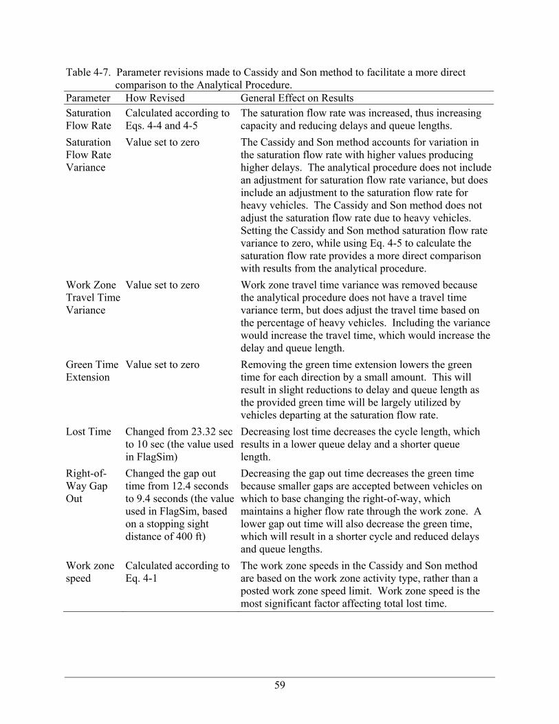
4-5 Parameter revisions made to Cassidy and Son method to facilitate more direct comparison to the Analytical Procedure. ...........................................................................59
4-6 Comparison of Cassidy and Son with FlagSim and generated models .............................60
4-7 Comparison of uniform delay and queue length equations ...............................................61
LIST OF FIGURES
3-1 Two-lane work zone operated with flagging control. ........................................................37
3-2 K value location used in simulation. ..................................................................................37
3-3 Screen shot of the program main user interface .................................................................38
3-4 Screen shot of vehicle parameter setting window..............................................................38
3-5 Screen shot of the multiple run input form ........................................................................39
3-6 Screen shot of animation window ......................................................................................39
3-7 Relationship of work zone speed to capacity .....................................................................40
3-9 Relationship of green time to capacity...............................................................................40
3-10 Relationship of work zone length to capacity ....................................................................41
3-11 Relationship of heavy vehicle percentage to capacity .......................................................41
4-1 Model-estimated queue delay versus simulation queue delay. ..........................................56
4-2 Model-estimated queue length versus simulation queue length. .......................................57
A-1 Sample of the Summary Output File .................................................................................65
1
CHAPTER 1
INTRODUCTION
Background
With an aging roadway infrastructure and increase in city sprawl, construction work zones
are a common fixture on our roadway system. Work zone delays have a negative effect on not
only the transportation network, but also on the national economy, as well. On September 9,
2004, the Federal Highway Administration (FHWA) updated its ‘Work Zone Safety and
Mobility’ rule. This rule mandates that states develop an agency-level work zone safety and
mobility policy.
The states’ policies must include plans to minimize the congestion impacts to the public,
and address all types of roadway facilities and construction operations on a corridor, and network
level. From freeways to rural two-lane roads, each construction project must develop a plan to
lower the cost of congestion. Over the past 20 years, there have been numerous research projects
on estimating motorist delays for freeway work zones. However, few research projects have
been conducted on two-lane, two-way roadway work zones. Such work zone configurations
consist of a single lane that accommodates both directions of flow, in an alternating pattern.
These work zones typically employ a flagging control person (i.e., someone who operates a sign
that gives motorists instructions to stop or proceed) at both ends to regulate the flow of traffic
through the work zone. In some situations (usually where the lane closure is long or there are a
large number of driveways), a lead vehicle, called a pilot car, may be required to lead the platoon
of vehicles through the work zone.
Problem Statement
Previous to this research project, there was not a single accepted national standard for
analyzing work zone operations and estimating performance measures, particularly for two-lane,
2
two-way roadways. As a result, transportation agencies were required to develop their own
method or adopt/adapt one from existing methods. However, there were a limited number of
methods available. The Highway Capacity Manual (HCM) (2000) provides some guidance on
work zone analysis, but only for freeway facilities. A software product, called QuickZone, is
publicly available, but the level of support and lack of technical documentation (particularly with
respect to two-lane, two-way work zone configurations) has diminished its widespread
acceptance. The Florida Department of Transportation (FDOT) opted to develop their own
methodology because of these issues. The FDOT method currently used is a relatively simple
deterministic procedure, with rough approximations for work zone capacity and other important
parameter values. With ever-stricter guidelines on acceptable levels of traveler delay from
construction activities, it is essential that an analysis method be as accurate as possible. One of
the major limitations with most of the existing methods is the assumption of a fixed capacity
value, or a very narrow range of capacity values, for a variety of work zone scenarios. However,
for two-lane, two-way roadways, capacity is a function of saturation flow rate, work zone length,
travel time through the work zone, and green time given to each direction of flow. Therefore, to
achieve the goals of this project, it was necessary to develop a new procedure, or adapt an
existing one, which was more accurate, while still allowing for easy implementation. Meeting
these requirements will facilitate the traffic engineering community’s acceptance and utilization
of the developed method.
Research Objective and Supporting Tasks
The objective of this research was to develop a procedure to analyze two-way, two-lane
work zones and implement it in an easy-to-use format. More specifically, the procedure will
estimate capacity, delay, and queue length for varying work zone, traffic, and flagging
conditions. The tasks that were conducted to support the objective were as follows:
3
• Reviewed the literature to identify existing analysis procedures/methods.
• Reviewed the state of the practice of flagging operations.
• Identified alternative analysis methods that could be adapted for use in Florida.
• Developed a simulation program that calculates several measures of effectiveness for a variety of work zone scenarios, and provides visualization of the work zone operations.
• Developed saturation flow rate, work zone speed, queue delay, and queue length estimation models from the simulation data.
• Implemented the models in a spreadsheet format for application by practitioners/analysts.
Document Organization
In the following report, chapter 2 contains a summary of relevant literature and procedures
used by other agencies in analyzing two-lane work zones. Next, chapter 3 describes the research
approach, including simulation program development and experimental design. Chapter 4
contains a description of the model development and data analysis. Finally, chapter 5
summarizes the study, presents the conclusions reached, and topics for future research.
4
CHAPTER 2 LITERATURE REVIEW
Introduction
This chapter presents a summary of the review of relevant literature, discusses the
literature and proposes a methodology to be developed based on the review of the state of the
practice. Specifically, this review addresses two areas—previous research and the procedures
used in that research.
Background
In the literature review process, it was discovered that relatively little research had been
performed in the area of two-lane, two-way work zones with flagging operations. In contrast,
there had been significantly more research conducted on analyzing freeway work zones with lane
closures. The reason for this disparity may have resulted from federal government’s focus on
high traffic/congestion facilities. With the new work zone rule requiring all significant work
zone projects to have a traffic management plan, there was a need develop analysis methods for
two-lane, two-way roadways.
The Rule on Work Zone Safety and Mobility, developed in 2004, requires state and local
transportation agencies to have traffic management plans in place to mediate work zone related
congestion problems by October 2007. This rule states that all “Significant Projects” defined by
a state must have a plan from the beginning of the planning process. A “Significant Project” is
when certain locations where the congestion will create major delays or there are other projects
being performed in coordination, these need to be considered as significant. Two-lane, two-way
roadways do not automatically qualify as significant (FHWA, 2004). However, for a
transportation agency to be able to determine if a two-lane roadway work zone would create
significant congestion, it needed an accurate analysis method.
5
Previous Research
In this section, a summary of previous research is presented that pertains to the estimation
of traffic operations in two-lane, two-way work zones.
Cassidy and Son
Cassidy and Son (1995) developed a method to estimate the delays generated due to a lane
closure on a two-lane, two-way roadway. Their method consisted of a series of equations based
on stochastic queuing theory. The delays are primarily a function of traffic demand, travel time
through the work zone, and green time. They assessed the validity of their method through both
Monte Carlo simulation and microscopic simulation. They concluded that the method
“adequately predicts the impacts”.
The series of equations comprising Cassidy and Son’s method are largely based on
previously developed equations for analyzing operations at signalized intersections. The sources
for these previously developed equations included: 1) Webster (1966) for queue delay estimation
at a signalized intersection; 2) Newell (1969) for one-way vehicle-actuated signalized
intersection operations; and 3) Ceder and Regueres (1990) who obtained average work zone
delays from simulation and then compared those results to average delay from Webster’s
equations.
The development of their calculation procedure using equations that account for the
stochastic nature of traffic operations in these work zones was based on previous efforts that
investigated equations based on both deterministic and stochastic processes (Cassidy and Han,
1993; Cassidy, et al., 1994).
An overview of the Cassidy and Son calculation procedure is provided below. The outline
lists the required parameters; the work zone types that can be evaluated, and how oversaturated
conditions are handled.
6
Calculation procedure outline
1. For under-saturated conditions, estimated delay is a function of: a. work zone length b. work zone speed c. queue discharge rate d. traffic demand e. “red” time
2. For over-saturated conditions, delay is a function of the above factors, and calculated with deterministic queuing equations
3. Work zone types a. Asphalt overlays (w/ pilot car) b. Chip-Seal (w/ pilot car) c. General construction (w/ pilot car) d. General construction (w/o pilot car)
Field data
The data for Cassidy and Son’s research consisted of using 15 field sites in California. The
field data obtained from these sites were used as the basis to develop parameter values for the
four different work zone types listed above. Parameters such as the mean and variance of queue
discharge rate, the mean and variance of speed through the work zone, lost time, green time
extension, and variance to mean ratios of arrivals and departures were estimated for each of the
four work zone types. One issue with their field data is that none of the traffic demand rates
were large enough for them to determine the actual capacities of these work zone configurations.
While capacity can be determined indirectly through the measured saturation flow rates and
proportions of “green” time, these values could not be verified against actual field-measured
capacity values.
Another potential issue is that at 10 of the 15 field sites, a pilot car was used. The purpose
of a pilot car is to lead the queued traffic through the work zone area. Certainly, the presence of
a pilot car can have additional impacts beyond that of only flagger control. The Manual on
Uniform Traffic Control Devices (MUTCD) (2003) does not offer any guidance on when pilot
cars should be used in a work zone. If the work zone is complex or the flaggers do not have a
7
clear sight of the work zone, then a pilot car is usually considered. In Florida, at least, the use of
pilot cars at two-lane, two-way work zones appears to be quite rare.
In their proposed calculation procedure, the start-up lost time is a constant value, rather
than a random variable, for a given work zone type. They hypothesize that since lost time is
typically a small percentage of the overall cycle length, treating it, as a constant value will only
introduce a negligible amount of error into the delay estimation. This assumption seems
reasonable.
Although their delay estimation equation accounts for green time extension (i.e., green
time provided after the dissipation of the initial queue), they found that the contribution of this
term to the delay estimation was negligible due its small percentage of the cycle length. The
“gap-out” time (i.e., headway threshold) that was utilized to estimate the green time extension
was a constant value of 12.2 seconds, estimated, again, from empirical data. In other words, the
green time is assumed to extend for as long as vehicle arrival headways are less than 12.2
seconds. Although Cassidy and Son did not find a relationship between extended green times
and the arrival rates, they theorized that the values were a function of the arrival rate. This
observation may have been a function of the inherent variance in flagger operations.
Simulation data
Cassidy and Son’s initial efforts in developing a calculation procedure utilized
deterministic equations that assumed uniform arrival and queue discharge rates. They then tried
to extend these equations by employing Monte Carlo simulation to generate key parameter
values for the equations from statistical distributions based on empirical data. While the results
of this exercise were more plausible for the stochastic nature of these work zone operations, it
still had several significant limitations.
8
This ultimately led them to the adaptation of equations previously developed for modeling
vehicle-actuated signalized intersections. These equations generally account for the stochastic
nature of work zone operations. They also wrote a relatively simple microscopic simulation
program for testing the validity of the analytical equations. They found that the equations based
on vehicle-actuated signalized intersection operations provided the best match with the
microscopic simulation results, relative to the equations based on constant values or with values
determined from Monte Carlo simulation.
FDOT Procedure
The FDOT developed a lane closure analysis procedure for use with all road type classes.
The procedure is in the Plans Preparation Manual (PPM), Volume I, Section 10.14.7 (2006). The
procedure can analyze two-lane two-way work zones. In order to accommodate flagging
operations, the procedure attempts to determine the peak hour volume and the restricted capacity.
From these two values, the time during when lane closures can occur without creating excessive
delays is determined.
This procedure’s main limitation is that capacity is an input, and the given capacities were
not specific to two-lane work zones. With capacity not based on a flagging work zone value, the
procedure quite likely will be unable to model the field conditions accurately. Another limitation
with modeling flagging operations with this procedure is that it is based on only the ratio of
green time to the cycle length. This assumption does not take in to account the differences in
delays of flagging operations, such as the lost time due to the traversing the work zone, startup
lost time and the variation of extended green time.
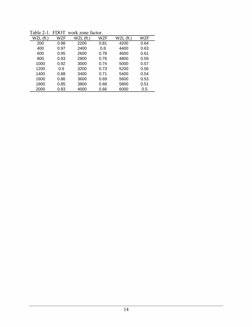
The capacity is adjusted by the work zone factor (WZF) shown in Table 2-1. The WZF is
used instead of a calculated travel time based on a typical speed. All of the lost time is also
incorporated in to the WZF. This is a simplistic adjustment to incorporate these important
9
factors. The travel time through the work zone is an easy calculation, which would make a
logical factor. One of the problems is the WZF is not adjusted by speed and is not documented
by what speed the factor is based on. This is an important question, as speeds through a work
zone can be quite different for an intense construction operation like chip and seal versus a less
intense operation such as shoulder work.
The FDOT PPM lane closure analysis procedure is as follows:
1. Select the appropriate capacity (c) from the table below:
LANE CLOSURE CAPACITY TABLE
Capacity (c) of an Existing 2-Lane-Converted to 2-Way, 1-Lane=1400 veh/hr
Capacity (c) of an Existing 4-Lane-Converted to 1-Way, 1-Lane=1800 veh/hr
Capacity (c) of an Existing 6-Lane-Converted to 1-Way, 1-Lane=3600 veh/hr
Therefore, for a two-lane highway work zone, the capacity (c) is 1400 veh/hr.
2. The restricted capacity (RC) is then calculated taking into consideration the following
factors:
TLW = Travel Lane Width
LC = Lateral Clearance. This is the distance from the edge of the travel lane to the obstruction (e.g., Jersey barrier)
WZF = Work Zone Factor is proportional to the length of the work zone. This factor is only used in the procedure for two-lane two-way work zones.
OF = Obstruction Factor. This factor reduces the capacity of the travel lane if the one of the following factors violates their constraints: TLW less than 12 ft and LC less than 6 ft.
G/C = Ratio of green time to cycle time. This factor is applied when the lane closure is through or within 600 ft of a signalized intersection.
ADT = Average Daily trips this value is used to calculate the design hourly volume.
The RC for roadways without signals is calculated as follows:
RC (Open Road) = c × OF × WZF
10
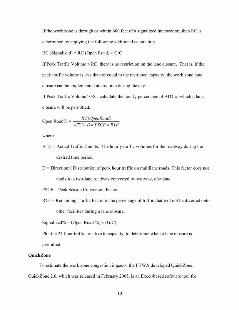
If the work zone is through or within 600 feet of a signalized intersection, then RC is
determined by applying the following additional calculation.
RC (Signalized) = RC (Open Road) × G/C
If Peak Traffic Volume ≤ RC, there is no restriction on the lane closure. That is, if the
peak traffic volume is less than or equal to the restricted capacity, the work zone lane
closure can be implemented at any time during the day.
If Peak Traffic Volume > RC, calculate the hourly percentage of ADT at which a lane
closure will be permitted.
Open Road% = RTFPSCFDATC
OpenRoadRC×××
)(
where
ATC = Actual Traffic Counts. The hourly traffic volumes for the roadway during the
desired time period.
D = Directional Distribution of peak hour traffic on multilane roads. This factor does not
apply to a two-lane roadway converted to two-way, one-lane.
PSCF = Peak Season Conversion Factor
RTF = Remaining Traffic Factor is the percentage of traffic that will not be diverted onto
other facilities during a lane closure.
Signalized% = (Open Road %) × (G/C)
Plot the 24-hour traffic, relative to capacity, to determine when a lane closure is
permitted.
QuickZone
To estimate the work zone congestion impacts, the FHWA developed QuickZone.
QuickZone 2.0, which was released in February 2005, is an Excel-based software tool for
11
estimating queues and delays in work zones. The maximum allowable queues and delays are
calculated as part of the procedure in optimizing a staging/phasing plan and developing a traffic
mitigation strategy. As a result, lane closure schedules are recommended to minimize user costs.
This is a quick and easy method, with a user-friendly, concise spreadsheet setup. (Arguea,
2006).
The QuickZone method requires the following input data:
• Network data - Describing the mainline facility under construction as well as adjacent alternatives in the travel corridor, which can be used to calculate the traffic diversion
• Link capacity - Each link has its own capacity value for vehicles per hour
• Project data - Describing the plan for work zone strategy and phasing, including capacity reductions resulting from work zones
• Travel demand data - Describing patterns of pre-construction corridor utilization
• Corridor management data - Describing various congestion mitigation strategies to be implemented in each phase, including estimates of capacity changes from these mitigation strategies
QuickZone has a module for flagging operations. The procedures are similar to other
roadway types handled within the program. However, for flagging operations, QuickZone is
limited in several areas. One limitation is that if the work zone is over a mile in length, it
assumes the use of pilot cars, which adds an additional lost time factor. Another limitation, per
se, is that user interface for the two-lane work zone analysis is cumbersome at best, making the
data input process very difficult. An additional limitation was the lack of control on the flagging
operation. QuickZone requires a pilot car with work zones longer than 1.0 miles, and maximum
green time cannot be adjusted—an important policy decision in work zones near or over
capacity. Another limitation was, unfortunately, very limited documentation on the analysis
procedure and justification for selected parameter values. A thorough review of QuickZone’s
internal calculations procedure written in Microsoft Excel VBA® was performed, and from this,
12
it was determined that the two-lane work zone procedure was inadequate for the needs of this
project.
Colorado DOT
The Colorado DOT “Lane Closure Strategy” (2004) was intended to give guidance on
scheduling lane closures on two-lane work zones. Capacity values were determined by the
probability of a cycle failure (inability to serve all vehicles) based on a Poisson distribution. It
was assumed that some cycles would fail, so a 10% failure rate was allowed. For their analysis,
it was determined that 60 seconds was an appropriate “green time” for each direction. The
capacity determined for a 10% failure rate results in an average of 22.2 vehicles through the
work zone in each direction per cycle. The speed limit through the work zone was assumed to be
30 mi/h. The travel time through the work zone was calculated based on a loaded semi-truck
accelerating to 30 mi/h. This results in 34 one-way cycles per hour for the 0.25-mile closure and
18 cycles for the 1.0-mile closure. The resulting hourly capacity calculated for a work zone in
flat terrain was 755 veh/h for a 0.25-mile work zone and 400 veh/h for a 1.0-mile work zone.
This analysis is a simple approximation of the field conditions. Flagging variations were
not taken into account, and the time to traverse the work zone used the acceleration value from a
semi-truck, which can be the limiting condition in certain scenarios. One critical assumption
made was a 60-second green time. This green time was most likely used because the model
formulation was based on a delay formulation for signalized intersections, with an upper limit of
72 seconds of green time. With these assumptions, the Colorado DOT model estimates lower
capacity values than the Cassidy and Son (1994) method.
Summary and Conclusions
The literature review explored existing methods/models that were used to estimate capacity
and delays for two-lane work zones with flagging operations. However, only a limited number
13
of research projects on this topic have been conducted to date, and it is evident that additional
research is still needed fully understand work zone operations under flagging operations.
• All methods/models examined either use a single, or a very limited number of capacity values.
o While the Cassidy and Son method calculates capacity from the saturation flow and green time proportion, they still only use four different values of saturation flow rate (and those only range in value from 1018 veh/h to 1090 veh/h). Obviously, capacity is the most influential factor in work zone operational quality, if not all roadway facility types. Ideally, capacity (or possibly saturation flow rate) should be estimated for the specific combination of work zone conditions being analyzed to more accurately estimate delays and queue lengths. For the existing methods/models, there are clearly many combinations of work zone conditions that result in significantly different capacity values than those “built-in” to the method. Even the Cassidy and Son field data found a range of saturation flow rates from 750 to 1450 veh/h.
o FDOT PPM uses a capacity value of 1400 veh/h
• With QuickZone’s limited documentation on development and procedures used for two-lane work zone analysis, the program is difficult to implement into a traffic management plan for two-lane work zones. The significant weakness with QuickZone is the requirement for the user to input a capacity. With no guidance, the user has to make their best guess, which could potentially be significantly inaccurate.
• The Colorado Department of Transportation procedures were overly conservative and did not provide much flexibility to the user to adapt the methods to a particular location. Without much flexibility to be adapted to specific locations, this method was too limited to be further developed to implement in Florida.
• Besides the Cassidy and Son research, the available methods generally provide little technical documentation about the method and/or the derivation of parameter values used in the method. Furthermore, other than the Cassidy and Son study, there is a general lack of field data that have been collected to validate any of the developed methods. However, even with the Cassidy and Son data, most of the field data were obtained from sites using a pilot car and operations levels were generally well below capacity.
This chapter describes the research approach adopted to find the capacity, delays, and
queue lengths in two-lane two-way work zone configurations. More specifically, it discusses the
methodological approach, field observations, simulation model development, and the simulation
experiments. Also included is description of the sensitivity analysis employed to discover the
key variable ranges used in the experimental design.
Methodological Approach
The typical work zone flagging operation configuration consists of a single lane that
accommodates both directions of flow, in an alternating pattern. Figure 3-1 shows a typical two-
lane work zone with a lane closure. These work zones predominately use a flag person (i.e.,
someone who operates a sign that gives motorists instructions on whether to stop or proceed) at
both ends to control the flow of traffic into the work zone. Significant delay is incurred by
motorists due to the lost time that accrues while the opposing direction has the right-of-way.
Additionally, both directions incur lost time when there is a change in the right-of-way as the last
vehicle that received the right-of-way must traverse the entire length of the work zone; therefore,
all vehicles must wait until the last vehicle has passed the opposite stop bar. The queue
discharge is similar to the operation of a signalized intersection, but the lane switch along with
the proximity to construction activity would have an affect on the discharge rate.
Changing of the right-of-way is rarely performed in an optimal manner. Flaggers are not
trained on how to switch the right-of-way in such a manner as to minimize delay, or otherwise
optimize some particular performance measure (Evans, 2006). Generally, flaggers change the
flow direction due to queue and cycle length. The queue at the beginning of the “green” period
16
discharges at the saturation flow rate. After the initial queue dissipates, flaggers usually extend
the green to allow for vehicles still arriving. This extension time can be lowered if there is a
significant queue in the opposite direction. At this point, the flow through the work zone will
drop to the arrival rate. The arrival rate can be significantly lower than the queue discharge rate
on low volume roadways, thus increasing the overall average delay if vehicles are queuing at the
opposite approach (Cassidy and Son, 1994).
The standard performance measures for a work zone with flagging operations are:
• Capacity – maximum vehicle throughput • Delay – time spent not moving, or at a slower speed than desired • Queue lengths – vehicle arrivals minus vehicle departures for a specified length of time
Ideally, the operational impacts of these work zone configurations should be studied at
field sites resulting in a dataset that could be used to develop a methodology for estimating two-
lane work zone capacity. At the field sites, the factors that contribute to the capacity degradation
could be extensively examined. These factors could be used to provide additional insight into
the results of a simulation study. There would be a large number of different work zone
scenarios encountered in the field. Consequently, there are two complications to collecting field
data from all of these scenarios: 1) It is not possible to find all such scenarios within a reasonable
distance and within the project period, and 2) the project budget does not allow for field data
collection at a large number of sites.
Therefore, the approach chosen was to use simulation data for the analysis procedure
development. However, a limited number of informal field observations were performed to have
an understanding of their operations. These sites gave an idea of how the work zones were
controlled.
17
Simulation
To generate the data for developing the analysis procedure a work zone simulation was
used. Using a simulation program provides the ability to test a much larger variety of traffic and
work zone configuration conditions than would normally be possible from the amount of field
data collected within the normal timeline and resources of a project.
Two-lane work zones are unique in their operation. In order to estimate the operation a
number of factors are required. The following capabilities were necessary to simulate two-lane
work zones:
• model a variety of flagging control methods • model vehicle arrivals at the work zone • model vehicles discharging from the stop line • model heavy vehicles, in addition to passenger cars • model vehicles traveling through the work zone • record various simulation results in order to allow for the following performance
measures to be calculated o Lost time due to right-of-way change o queue delay o travel time delay due to reduced speeds o queue length o capacity
A review of existing commercially available simulation packages was made to determine if
any were readily applicable to this situation. VISSIM, CORSIM, AIMSUM, and PARAMICS
do not explicitly provide for modeling of work zones on two-lane roadways. The key to this
research project was the ability to model the flagging control. Each program could be used to
change to from green to red, using different detector settings. However, what prevents the
implementation of other software packages was the inability for the available programs to track
the last vehicle through the work zone. This feature was needed in order to begin the green
period for the opposite direction.
18
Additionally, it was required to have more ability to control inputs and outputs. Additional
control over the arrangements of inputs and outputs allows for more efficient running of the
simulation scenarios and more efficient processing of the results. A lack of technical
documentation detailing the underlying methods/models was also problematic for several
commercially available simulation models.
Program Development
The simulation program that was developed, called FlagSim, is a Windows-based
application written with the Visual Basic 2005 language. FlagSim is a microscopic, stochastic
simulation program that models the arrival of vehicles to the work zone, the discharge of
vehicles into the work zone area, and the travel of these vehicles through the work zone area.
From this program, the capacity of the work zone, and delays imparted to the motorists were
calculated. The purpose of the program was to realistically model traffic operations in work
zone areas using flagging operations and use the results of the data analysis from simulation to
develop an analytic computational procedure to estimate pertinent performance measures.
Vehicle distribution
For each simulation run, a unique set of vehicles was created. This set of vehicles can be
defined by the user, given a variety of inputs defined in FlagSim. To choose the vehicle set, a
vehicle generator selects from four different vehicle types. The selection was randomly
generated, based on user-specified vehicle proportions. Four vehicle types were available within
the simulation program: 1) passenger cars, 2) small trucks, 3) medium trucks, and 4) large trucks.
For these vehicle types, the user also has the ability to adjust the properties of each vehicle type
to fit a particular traffic pattern.
19
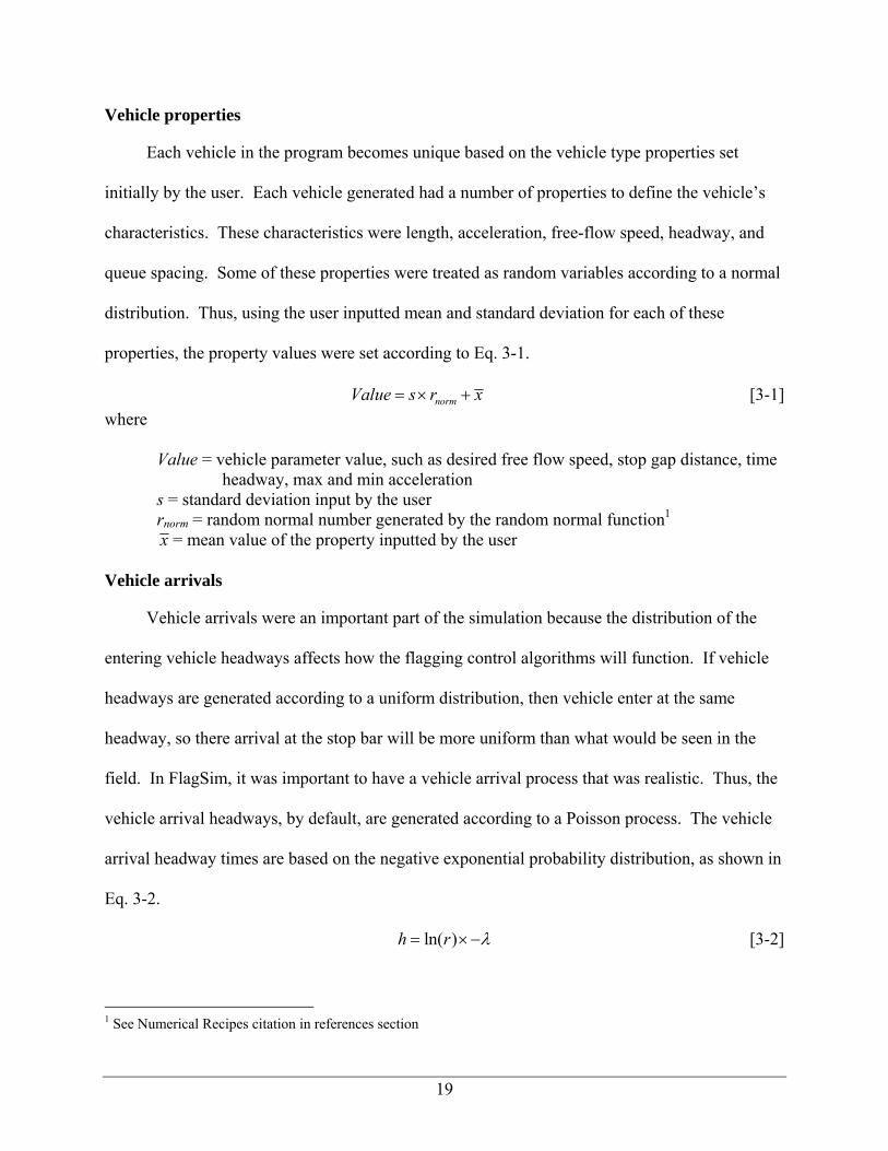
Vehicle properties
Each vehicle in the program becomes unique based on the vehicle type properties set
initially by the user. Each vehicle generated had a number of properties to define the vehicle’s
characteristics. These characteristics were length, acceleration, free-flow speed, headway, and
queue spacing. Some of these properties were treated as random variables according to a normal
distribution. Thus, using the user inputted mean and standard deviation for each of these
properties, the property values were set according to Eq. 3-1.
normValue s r x= × + [3-1] where
Value = vehicle parameter value, such as desired free flow speed, stop gap distance, time headway, max and min acceleration
s = standard deviation input by the user rnorm = random normal number generated by the random normal function1 x = mean value of the property inputted by the user
Vehicle arrivals
Vehicle arrivals were an important part of the simulation because the distribution of the
entering vehicle headways affects how the flagging control algorithms will function. If vehicle
headways are generated according to a uniform distribution, then vehicle enter at the same
headway, so there arrival at the stop bar will be more uniform than what would be seen in the
field. In FlagSim, it was important to have a vehicle arrival process that was realistic. Thus, the
vehicle arrival headways, by default, are generated according to a Poisson process. The vehicle
arrival headway times are based on the negative exponential probability distribution, as shown in
Eq. 3-2.
ln( )h r λ= ×− [3-2]
1 See Numerical Recipes citation in references section
20
where
h = vehicle headway, in seconds r = random number generated from a uniform distribution2 λ = average arrival rate, in veh/sec ln = natural logarithm
Upper and lower bounds were also applied to the generated headway values. Extremely
high headway values will lead to significant differences between the input volume and the
simulation volume. Extremely low headway values are not realistic due to drivers’ general
desire to maintain a safe following distance. The lower bound was set to 0.5 seconds. The upper
bound was set to a value of four times the average vehicle arrival rate. These values resulted in
the simulated volumes reflecting the input traffic volumes. The program has the capability to
allow the user to select a uniform arrival rate. The uniform arrival rate was used for calibration
to compare procedures that are based on uniform arrivals.
Initial speed
After a vehicle was generated into the network, the initial speed of the vehicle was set.
The desired speed of the vehicle was its free flow speed determined during the setting of the
vehicle’s properties. A vehicle’s speed was initially set to the free flow speed. In some cases, a
vehicle that enters at its desired speed could collide with the lead vehicle. A check was
performed to determine if the vehicle was too close to its lead vehicle. If the distance between
vehicles was too close then the vehicle’s speed was set to the current speed of the lead vehicle
with an acceleration of zero.
2 This value is generated from the ‘Rnd’ function within Visual Basic 2005, which generates pseudo-random numbers between 0 and 1 according to a specific algorithm. http://support.microsoft.com/kb/q231847/
21
Car-following model
The car-following model was an important component of the simulation program. The
car-following model was the mathematical foundation of the computations that described the
movement of vehicles through the specified roadway system. The selection of a car-following
model for this program was based on specific criteria. The queue discharge aspect of traffic flow
in the work zone area was the most critical element to the validity of the simulation results.
Therefore, the model selected had to be particularly suitable for modeling the queue discharge
phenomenon. After review of various models, the Modified-Pitt car-following model (Cohen,
2002) was selected for implementation. The Modified-Pitt car-following model was
demonstrated by Cohen (2002) and Washburn and Cruz-Casas (2007) to work well for queue
discharge modeling situations. For more discussion on queue discharge models, refer to
Washburn and Cruz-Casas (2007).
The Modified Pitt car-following equation calculates the acceleration value for a trailing
vehicle based on intuitive parameters such as the speed and acceleration of the lead vehicle, the
speed of the trailing vehicle, the relative position of the lead and trail vehicles, as well as a
desired headway. This equation also incorporates a sensitivity factor, K, which will be discussed
later in more detail. This equation allows for relatively easy calibration. Car-following models
are generally based on a ‘driving rule’, such as a desired following distance or following
headway. The Modified Pitt model is based on the rule of a desired following headway.
As indicated before, the acceleration of each vehicle depends of the leading and trailing
vehicle and this model takes into consideration the physical and operational characteristics of
both. The main form of the model is shown in Eq. 3-3.
22
2
( ) ( ) ( )
1[ ( ) ( )]2 ( )
( ) 1( )2
l f l f
f ll
f
s t R s t R L hv t RK
v t R v t R Ta t T T
a t TT h
T
+ − + − − + +⎧ ⎫⎪ ⎪⎨ ⎬+ − + −⎪ ⎪+⎩ ⎭+ =
+ [3-3]
where
af(t+T) = acceleration of follower vehicle at time t+T, in ft/s2 al(t+R) = acceleration of lead vehicle at time t+R, in ft/s2 sl(t+R) = position of lead vehicle at time t+R as measured from upstream, in feet sf(t+R) = position of follower vehicle at time t+R as measured from upstream, in feet vf(t+R) = speed of follower vehicle at time t+R, in ft/s vl(t+R) = speed of lead vehicle at time t+R, in ft/s Ll = length of lead vehicle plus a buffer based on jam density, in ft h = time headway parameter (refers to headway between rear bumper plus a buffer of lead
vehicle to front bumper of follower), in seconds T = simulation time-scan interval, in seconds t = current simulation time step, in seconds R = perception-reaction time, in seconds K = sensitivity parameter (unitless)
For application to this project, the value of the L parameter varied based on one of the four
different vehicle types. The time headway parameter (h) was set as a random variable, rather
than a constant value, to introduce an additional stochastic element to the model. The value of
the vehicle headway was based on a normal distribution to represent the more realistic scenario
that desired headways vary by driver. The mean and standard deviation for this distribution can
be specified for each of the four vehicle types. Thus, desired headways can vary by driver, as
well as by vehicle category.
The perception-reaction time, R, and the simulation time-scan interval, T, are important
parameters. Considerable time was spent experimenting with different values for each.
Ultimately, both values were set to 0.1 seconds. This value for the time-scan interval provided
for very detailed vehicle trajectory data, which enabled very accurate measurements to be made
of the measures of effectiveness, and enabled smooth vehicle animation in the work zone
23
visualization screen. While a perception-reaction time of 0.1 seconds may seem intuitively low,
it was found that this led to the most realistic traffic flow representation. Individual perception-
reaction times are undoubtedly higher than this for any isolated event. However, the fact is that
real-life traffic flow happens on a continuous time scale, and real-life drivers make continuous
incremental acceleration and deceleration (as well as steering) inputs, withstanding sudden
events/panic maneuvers. Thus, these constant incremental changes by both leading and
following vehicles generally results in smooth traffic flow. Again, this value of 0.1 seconds for
the time-scan interval and perception-reaction time resulted in this type of realistic traffic flow.
Queue arrival and discharge
The sensitivity parameter, K, has two separate values in the car-following model—one for
the queue arrival and discharge and for the travel through the work zone. Cohen stated that a
larger K value should be used in interrupted flow conditions due to over-damping effects (Cohen,
2002a). This assumption was tested in the car-following model and yielded the best results.
Vehicles had a smoother interaction in the work zone (uninterrupted flow) with K = 0.75 and for
the queue arrival and queue discharge processes performed well with K = 1.1. The definition of
the queue arrival area was 300 feet upstream of the last vehicle in queue, and the definition of the
queue discharge area was 300 feet downstream of the entering work zone stop bar.
Another key parameter, for queue discharge, was the heavy vehicle acceleration rate. The
truck acceleration rate was based on work by Rakha and Lucic (2002), from which a constant
value of 1.5 ft/sec2 was selected for implementation in FlagSim. From a visual inspection of the
animation, and review of vehicle trajectory data, this value resulted in reasonable truck
headways.
24
Flagging operations
A significant feature of FlagSim was the ability to specify several different methods by
which the right-of-way could be controlled. Changing of the right-of-way can be a complex
operation. A decision to change the right-of-way is generally based on several factors, such as
the amount of traffic that needs to be served in each direction of travel, the time it takes to travel
the work zone, and policy considerations such as maximum queue length or maximum green
time. A flag change, much like a phase change at a signalized intersection, has a lost time
associated with it. For the work zone to operate efficiently, the right-of-way must not be
switched too often such that the lost time becomes a significant portion of the cycle length.
Additionally, the flagging method employed at a work zone site is almost guaranteed not to
result in optimal condition; for example, minimizing vehicle delay. This non-optimal condition
is a direct result of the flag operators allocating non-optimal amounts of green time. Cassidy and
Son (1994) stated that the green time was most often extended past the optimal time that should
be given to each direction.
Startup lost time
Startup lost time begins when the front bumper of the platoon’s last vehicle crosses the
stop bar exiting the work zone and ends when the front bumper of the vehicle entering work zone
crosses the stop bar. This lost time is caused by several factors. The first delay occurs as the last
vehicle exiting the work zone travels from the work zone exit point to a safe distance in order to
allow the next direction of vehicles to proceed. The exiting vehicle must maneuver the lane
switch area and pass the first few vehicles queued. Second, an additional time is needed for the
flagger to perform the flag change, such as the time it takes the flagger to determine when the
work zone is clear. Finally, there is lost time for the first vehicle reacting to the change of the
sign, similar to vehicles’ startup lost time at a signalized intersection. In addition, since this lost
25
time is random in the field, the program accounted for this randomness by modeling it with a
normal distribution, using a mean of 10 seconds and a standard deviation of (+/-) 2 seconds. The
randomness accounts for variation with the flaggers and variation in drivers’ reaction to the
changing of the flag. The first vehicle was delayed the calculated amount of time before
beginning to proceed into the work zone.
Flagging methods
FlagSim contains a variety of flagging methods to try to encapsulate the various methods
operators might use to control two-lane work zones. The flagging control methods are generally
based on control strategies used in traffic signal operations. The following flagging methods are
implemented in FlagSim.
• Distance Gap-Out: Right-of-way change is based on specified distance gap between approaching vehicles.
• Queue Length: Right-of-way change is based on a maximum queue length of vehicles on the opposing approach.
• Fixed Green Time: Right-of-way is changed after the specified fixed green time is reached. This flagging method can also be used in combination with the distance gap-out, and queue length methods, subject to a maximum green time.
User Interface
The user interface was designed to allow the user to quickly and easily use the program.
To accomplish this, multiple input forms were incorporated. The main user form is shown in
Figure 3-3. In this form, the user is able to select the most common program inputs. The main
form gives the user the ability to quickly edit a single run and generate the results and animation.
More detailed user inputs are contained in the ‘Vehicle Parameter Settings’ form (Figure 3-4);
however, it is not intended that these values be changed unless the analyst has specific data for a
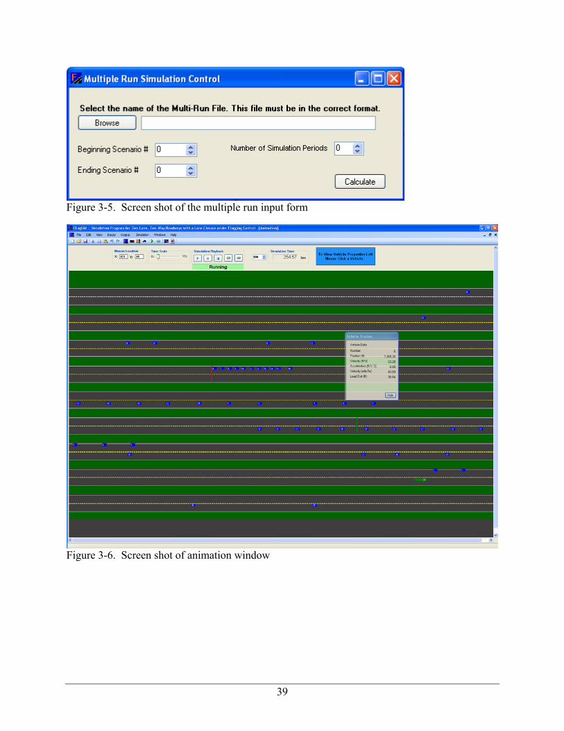
site contrary to these values. To facilitate multiple runs of a given scenario, the ‘Multiple Run
Simulation Control’ input form (Figure 3-5) is provided.
26
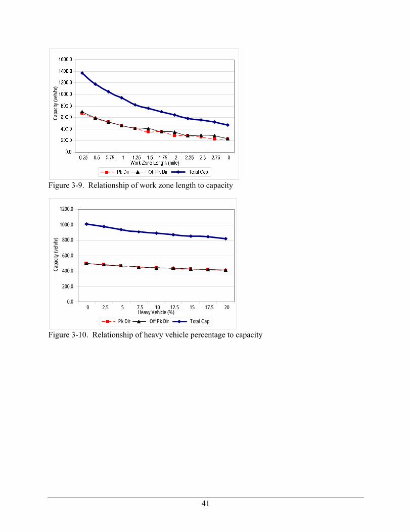
Animation
FlagSim incorporates a 2-D post-processor animation viewer, shown in Figure 3-6. The
animation allows the user to view the computations previously performed. Viewing the
animation gives the user an opportunity to review the simulation scenario visually. Items that
can be easily checked are vehicle generation, car-following interaction, and the flagging
variations.
At the top of the screen are the controls, which allow the user to control the animation—
play, pause, stop and speed control. One feature of the animation is the vehicle-tracking
window, shown in Figure 3-6. A small pop-up window appears if the user left-mouse clicks on a
vehicle. This window displays all of the time-step by time-step vehicle trajectory information
for the selected vehicle.
Outputs of the simulation
Since FlagSim is a microscopic simulation program, detailed vehicle trajectory data (i.e.,
acceleration, velocity, and position values) are generated at each time step. These data can be
saved to a time step data (TSD) file if the user so desires, in which case one TSD file per travel
direction is created. From the detailed time step data, several performance measures can be
calculated for the desired analysis period. These include:
• Total delay – The queue delay and the travel time delay accumulate for the entire simulation period.
• Average delay per vehicle – The total delay divided by the number of vehicles exiting the work zone during the simulation period.
• Average queue delay – The average delay of vehicles spent in a queue at the entrance to the lane closure area. For this project, queue delay was accumulated for any vehicle traveling less than 10 mi/h. Thus, this measure represents a hybrid queue delay between the traditional measures of stop delay (where delay is only accumulated when vehicle velocity equals zero) and control delay (where delay is accumulated for a vehicle any time its velocity is less than the average running speed). The value of 10 mi/h was a
27
compromise value to try to capture delay for those vehicles that were decelerating or stopped due to queuing, and not slowing just due to regular traffic flow conditions.
• Average cycle maximum back of queue (veh/cycle) – The average of the all the maximum back of queue lengths for each cycle. It should be noted that this queue length is in terms of number of vehicles, and is the absolute maximum back of queue (which accounts for vehicles arriving on green at the back of the initial queue at the start of green).
• Maximum back of queue (veh/simulation period) – The maximum back of queue length that occurs during the entire simulation period; that is, across all cycles.
• Average travel time delay through the work zone – Travel time delay was calculated based on the time the vehicle enters the work zone and the time it exits the work zone at the opposite crossbar compared to the time the vehicle would have traveled through the work zone if no work zone were present.
• Average time spent in the system – The total time a vehicle spends in the entire system from start of the warm up segment to a position 2000 feet passed the opposite stop bar. Only vehicles that have entered and completely exited the system are included in this measure.
• Maximum vehicle throughput (i.e., capacity) – The number of vehicles exiting the work zone. This is a function of the saturation flow rate, the green time, and the cycle length (which is a function of green time, start-up lost time, and travel time through the work zone).
• Average Cycle Length – Cycle length was measured from the beginning of green for one direction to the next beginning of green for the same direction. The average cycle length is calculated simply as the sum of all cycle lengths divided by the number of cycles in the simulation period.
• Average Green Time – The sum of all green periods, by direction, divided by the total number of green periods during the simulation period.
• Average g/C – The average g/C was the average of all g/C ratios for all cycles during the simulation period.
A summary file containing all these performance measures can be generated by FlagSim.
This file provided the input and output data that were used in the development of the
calculations/models for this project.
28
Simulation Calibration
For a simulation program’s output to be considered valid, it should be calibrated to match
real world situations. However, for this project, the resources were not available to perform field
data collection. To supplement this lack of field data, a quasi-calibration procedure was utilized,
which consisted of evaluating the reasonableness of traffic flow in three different modes: 1)
queue build-up, queue discharge, and uninterrupted flow through the work zone.
The queue build-up component of traffic flow was the most challenging to implement. To
have realistic vehicle movement, logic had to be implemented to ensure that a vehicle would
decelerate in time to avoid a rear-end collision, yet would not decelerate at an unreasonably high
rate (i.e., wait until the “last second” to slam on the brakes). Thus, the logic employed was such
that a vehicle would decelerate at a reasonable value (on the order of 10 ft/s2) when approaching
the stop bar or the back end of a queue. This assumption seems reasonable since drivers would
have an appropriate warning of the work zone ahead and would take enough precaution to slow
as directed by the work zone signage. Another assumption was that all vehicles, no matter how
far back in the queue, have enough warning to begin deceleration.
For the queue discharge component of traffic flow, results from an earlier research project
performed by Washburn and Cruz-Casas (2007) were utilized. For this project, an extensive
database of queue discharge headways was created. Forty-one hours of video data were
collected from six signalized intersections around central Florida. From the video data, queue
discharge headways were measured for the same four vehicle types as used in FlagSim. These
data provided a reasonable comparison data set because the queue discharge phenomenon at the
work zone stop bar is similar to the queue discharge phenomenon at a signalized intersection.
However, there can certainly be some differences, particularly for the traffic flow in the direction
of the closed lane (i.e., for the vehicles that have to perform a lane shift). To extract the headway
29
values from FlagSim, the program exported the first 10 vehicle headways from the beginning of
the green time. These data were compared to the data of Washburn and Cruz. FlagSim had an
average headway value of 2.01 seconds, which was reasonably consistent with the results from
Washburn and Cruz (2007).
For the uninterrupted flow of traffic through the work zone, visual inspection of the
simulation animation was performed. For this component of traffic flow, vehicle spacing was
the key factor analyzed. The initial platoon would eventually dissipate during travel. Each
vehicle has a different desired free-flow speed; therefore, slower vehicles would separate from
the leader and fall out of the car-following mode. This would happen to several vehicles; thus
result in a number of smaller platoons of vehicles. This phenomenon was also observed during
informal field site visits. In addition, proper implementation of the flagging control methods was
confirmed by visual inspection of the simulation animation.
Sensitivity Analysis
To determine the most appropriate variables to include in the experimental designs, which
were used to generate the data for model development, a sensitivity analysis was performed. The
objective was to identify variables that significantly affected capacity, delay, and queuing, as
well as the form of their relationship. Due to the computational time required for large
experimental designs, variables that did not have a considerable effect on work zone
performance were excluded from further consideration.
Each analysis scenario had the same base input values. From this base set of inputs, one
variable would then be varied over a given range. The base input values were as follows:
• Work zone length – 1 mile • Work zone speed – 40 mi/h • Posted speed – 40 mi/h • Heavy vehicles – 5 percent
30
• Max green time – 120 seconds • Traffic demand greater than capacity
Input traffic volumes were selected to insure that the traffic demand was greater than the
capacity. The results from the sensitivity analysis are provided in the following figures. The
thick line (with diamonds) represents the total traffic throughput (i.e., both directions) of the
work zone. The directional traffic flows are represented by the dashed line (with squares) and
thin solid (with triangles) lines.
Figure 3-7 shows the relationship of the work zone travel speed to capacity. This
relationship indicates that the slower the speed, the lower the capacity. This trend results from
the longer time it takes for a vehicle to traverse the work zone, and the additional lost time
incurred during the right-of-way change.
Figure 3-8 shows the relationship of green time to capacity. The green time value varied
from 30 seconds to 360 seconds. The capacity of the work zone increased with increased green
time given to each direction. The cycle length increases as the green time increases, which is
consistent with signalized intersection operations, and the longer the cycle length, the more
vehicles that can be served. This increase in capacity occurs because the percentage of lost time
for the cycle length is reduced. Travel time through the work zone during the right-of-way
change is the largest component of the lost time.
While increasing the green time does generally increase the capacity and lower the average
delay, it must be noted that a practical maximum green time should be implemented. While one
direction has the “green” indication, the other direction obviously has a “red” indication. The
longer the green for one direction, the more the queue length builds in the other direction during
red. Thus, the individual wait time will eventually reach an intolerable level, from a driver’s
perspective, as well as the queue length. At this point, the right-of-way must be switched, even
31
if it means less than optimal performance measure values. The assumption used in this project
was that 5 minutes was reasonable practical maximum green time. Shorter than optimal green
times may also be necessary when there are queue storage constraints, such as when the work
zone is close to an upstream intersection.
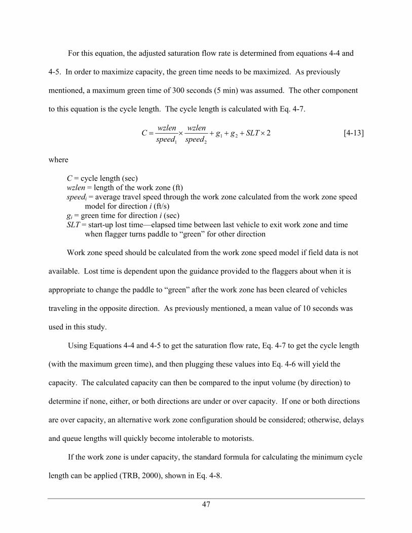
The relationship of work zone length to capacity is shown in Figure 3-9. It can be seen
that work zone capacity decreases as the length of the work zone increases. This decrease in
capacity can be explained by the increase in the time it takes the last vehicle to enter the work
zone on “green” to traverse the work zone, which results in additional lost time.
The relationship of heavy vehicle percentage to capacity is shown in Figure 3-10. An
increase in heavy vehicle percentage results in a decrease in capacity. Trucks decrease the queue
discharge rate, as well as lower the average speed of vehicles traveling through the work zone,
with both factors contributing to a decrease in work zone capacity.
Experimental Design
Arguably, the two most important measures of effectiveness at two-lane work zone sites
are delay (particularly queue delay) and queue length. The simulation program was used to
generate the data set upon which regression models for estimating these measures were based.
These models were incorporated into an analysis procedure for two-way, two-lane work zones.
Capacity, which is a function of several variables, is the single most influential parameter on
values of delay and queue length. The simulation program was also used to generate values of
capacity that would later be used to verify the saturation flow rate model and capacity
calculations based upon the model-estimated saturation flow rates.
Variable Selection
Two experimental designs were developed; one for generating capacity values and one for
generating queue delay and queue length data. For the development of the experimental designs,
32
the first step was to identify the variables that were expected to have significant influence on the
values of the performance measures. The following variables were selected for the capacity
experimental design based on the results from the sensitively analysis:
• Work zone length: Work zone length affects the travel time through the work zone, which in turn affects lost time and cycle length.
• Travel speed through the work zone: Travel speed affects the travel time through the work zone, which in turn affects lost time and cycle length. The speed downstream of a traffic “signal” stop bar has also been shown to affect the queue discharge rate at the stop bar.
• Percentage of heavy vehicles: Heavy vehicles affect two components of the traffic flow—the queue discharge rate and the travel time through the work zone. The queue discharge rate is affected because large trucks have a slower acceleration rate and consume more space in the queue. For travel through the work zone, trucks again consume more space on the roadway and have slower acceleration rates. Furthermore, truck drivers generally have lower desired travel speeds than passenger cars, presumably particularly so in a work zone area where lateral clearances are more constrained.
• Green time: Higher green times result in higher capacities. However, higher green times also result in longer cycle lengths and longer red times. As the red time increases with the green time, the resulting queue delays and queue lengths quickly reach intolerable levels from a driver’s perspective. Thus, as previously mentioned, it is usually necessary to implement a maximum acceptable green time.
Traffic volume was not a variable in the experimental design. To obtain capacity values, it
was necessary to specify a traffic demand that would exceed the expected capacity for the
specific combination of input variable values.
The same experimental design was used to generate data for both delay and queue length,
as the same variables affect both measures. Work zone length, work zone travel speed, and
percentage of heavy vehicles were also used in the queue delay/length experimental design.
Traffic volume was added to this experimental design, in the form of a total two-way volume and
a directional-split (D) factor, as traffic volume obviously has a very significant effect on queue
delay and queue length. The other variable added was a distance gap-out flagging method, as
explained in more detail as follows.
33
Several options were possible for the selection of green time values. One option is the
maximum green time, as was used for the capacity experimental design. This option is not very
realistic, as this maximum green time would only be used for capacity conditions. For situations
where the traffic demand is less than capacity, it is likely that smaller green times would be used.
Another option is to determine what cycle length is appropriate for each specific combination of
variables, and then proportion fixed green times for this cycle length according to the traffic
demands in each direction. This option, however, is not realistic for implementation in the field,
as flaggers cannot be expected to implement different fixed green times for the varying traffic
demands that occur throughout the lane closure period.
Another option is to have the flagger allocate just enough green time to serve the initial
standing queue at the beginning of the green period. This could also be combined with adding a
fixed amount of extended green time to serve vehicles that arrive at the back of the queue during
the green period. One challenge with this from a field implementation standpoint is that the
flagger may not always be able to see the back of the initial standing queue at the beginning of
green. In addition, implementing a fixed green time extension period would probably be difficult
for flaggers to implement given that it would be relatively short in duration and they would have
to continuously look at a watch or other timing device. Although the maximum green time
method employed for the capacity experimental design would also require a flagger to use a
timing device, they would not have to check it nearly as often due to the much longer timing
period. Furthermore, small errors (on an absolute basis rather than percentage basis) in the
actual timing used would not have as significant of an impact on the maximum green time
method as the short duration green time extension method.
34
Another option, and the one selected for the experimental design, is a distance gap-out
method with a maximum green time. With this method, green time is allocated until a specific
distance between arriving vehicles is exceeded at the entrance to the work zone, or the maximum
green time is reached. The distance gap-out method was implemented rather than a time gap-out
method (as often used in actuated signal control) because it was assumed that implementation of
a time gap-out method is very difficult to do with human flag operators. With the distance gap-
out method, a mark or cone can be placed at the appropriate distance and the flagger would be
instructed to change the right-of-way if there are no vehicles between that mark/cone and the
stop bar. This method also offers the potential to reduce vehicle delays relative to fixed timing,
as it is responsive to actual traffic demands, such as at vehicle actuated signalized intersections.
There is one disadvantage to this method for model development purposes, and that is that
the green time is not fixed from one cycle to the next. Therefore, the green time and cycle length
were recorded for each cycle during the simulation period to allow for calculating average g/C
ratios for each scenario.
The values chosen for the gap-out distance were based on a number of criteria. The first
being stopping sight distance values for the corresponding roadway speed approaching the lane
closure area, as given by Eq. 3-4. The second was the gap had to be long enough not to allow a
premature switch in right-of-way due to a gap forming in the queue. Gaps tended to form if the
first truck in queue was following a number of passenger cars. The third was that the value
could not be greater than the average arrival rate or the maximum green time would frequently
control.
rtVG
gag
V×
⎟⎟⎠
⎞⎜⎜⎝
⎛±⎟⎟
⎠
⎞⎜⎜⎝
⎛1
21 +
2 = SSD [3-4]
35
where
SSD = stopping sight distance (ft) a = deceleration rate (ft/s2) V1 = initial vehicle speed (ft/s) g = gravitational constant (ft/s2) tr = perception/reaction time (sec) G = roadway grade (+ for uphill and – for downhill) in percent/100
In this equation, a value of 1.0 second was used for the perception-reaction time and a
value of 10.0 ft/s2 was used for the deceleration rate. These values are the same as those
typically used for yellow-interval timing (ITE, 1999). Although AASHTO (2001) recommends
values of 2.5 seconds for perception-reaction time and 11.2 ft/s2 for deceleration rate for this
equation, it was felt that the yellow-interval timing values were more appropriate for this
situation where drivers are expecting to have to possibly come to a stop, whereas the AASHTO
values are more appropriate for unexpected stopping situations. The grade was assumed to be
level, which is generally appropriate for Florida conditions.
Even with this gap-out method, it should be noted that the maximum green time of five
minutes was also applied.
Setting Variable Levels
The second step in developing the experimental design was to determine the values that
will be used for the chosen variables. Two levels (i.e., values) for each variable are typical for
situations in which the relationships are linear in nature. If certain relationships are non-linear in
nature, then it is necessary to use three levels for each variable. If the relationship is not
predetermined to be linear, then it is usually prudent to use three levels. However, the size of the
experimental design (i.e., number of runs) will increase substantially in this case. This can be
illustrated with Eq. 3-5.
36
. FLR = [3-5]
where
R = Number of unique variable combinations (or simulation runs) L = Number of levels F = Number of factors
So for example, an experimental design with seven variables, each run at two levels, would
yield 32 (25) unique variable combinations, whereas an experimental design with seven
variables, each run at three levels would yield 243 (35) combinations. Thus, if it is known that
the relationships of interest are linear, there will be a substantial savings in computational time
versus the calculation time of a non-linear relationship.
The selected variables, and their setting levels, for the capacity and queue delay/length
experimental designs are shown in Table 3-1 and Table 3-2, respectively.
Number of Replications
The final step of the experimental design is to determine an appropriate number of
replications (i.e., runs of the simulation program) for each combination of variables in the
experimental design, to account for the stochastic nature of each simulation run.
The number of replications required is a function of the desired statistical confidence level,
the variance of the data, and the acceptable error tolerance. Eq. 3-6 can be used to calculate the
necessary sample size.
2
2 ⎟⎠⎞
⎜⎝⎛ ⋅=
εz
sn α/ [3-6]
where
n = minimum number of replications s = estimated sample standard deviation zα/2 = constant corresponding to the desired confidence level ε = permitted error
37
To determine an appropriate number of iterations, numerous test simulation runs were
made. The run-to-run variance was calculated for capacity, delay, and queue length. These
variance values were used in Eq. 3-5 with a 90% confidence level (zα/2 = 1.645) and error
tolerance of 5% of the variable of interest. From this exercise, it was determined that five
iterations were sufficient. Therefore, after choosing three levels for each of 5 variables, for a 35
experimental design, with 5 replications, a total of 1215 (243 × 5) simulation runs were required.
The next step in the project was to execute the experimental design with the simulation
program. The following chapter will describe the data analysis, model development, and
development of the calculations procedure based on the resulting simulation data.
Work Zone
Stop Bar
Stop Bar
Lane ShiftBack of Queue
Traversing work zone
Arriving vehicle
Length of Queue
Figure 3-1: Two-lane work zone operated with flagging control.
Figure 3-2. K value location used in simulation.
38
Figure 3-3. Screen shot of the program main user interface
Figure 3-4. Screen shot of vehicle parameter setting window
39
Figure 3-5. Screen shot of the multiple run input form
Figure 3-6. Screen shot of animation window
40
0.0
200.0
400.0
600.0
800.0
1000.0
1200.0
1400.0
25 30 35 40 45 50 55 60 65Work Zone Speed (mph)
Capa
city (
veh/h
r)
Pk Dir Off Pk Dir Total Cap
Figure 3-7. Relationship of work zone speed to capacity
0
200
400
600
800
1000
1200
1400
1600
1800
0 30 60 90 120 150 180 210 240 270 300 330 360
Green Time (sec)
Pk Dir Off Pk Dir Total Cap
Figure 3-8. Relationship of green time to capacity
41
Capa
city (
veh/h
r)
Figure 3-9. Relationship of work zone length to capacity
0.0
200.0
400.0
600.0
800.0
1000.0
1200.0
0 2.5 5 7.5 10 12.5 15 17.5 20Heavy Vehicle (%)
Capa
city (
veh/h
r)
Pk Dir Off Pk Dir Total Cap
Figure 3-10. Relationship of heavy vehicle percentage to capacity
42
Table 3-1. Experimental design variables and values for capacity data Settings
Factor Units Low Med High Work Zone Length (mi) 0.25 1.0 3.25 Work Zone Speed (mi/h) 20 35 50 Heavy Vehicles (%) 0 10 20 Green Time (sec) 60 180 300
Table 3-2. Experimental design variables and values for queue delay and queue length
estimation models Settings
Factor Units Low Med High Work Zone Length (mi) 0.25 1.0 3.25 Work Zone Speed (mi/h) 25 37.5 50 Heavy Vehicles (%) 0 10 20 Total Volume (veh/h) 400 700 1000 D-factor 0.5 0.6 0.7 Distance Gap-Out (ft) 325 450 550
43
CHAPTER 4 CALCULATION PROCEDURE DEVELOPMENT
Introduction
This chapter describes the development of models and calculations for work zone capacity,
delay and queue length. This is followed by a sample application of the calculation procedure.
Finally, a comparison of the results from this calculation procedure to those based on simple
deterministic equations and those based on the Cassidy and Son calculation procedure.
Work Zone Speed Model
The first model that was estimated was one for average work zone speed. With impact to
the overall cycle length due to the lost time caused by traversing the work zone, and impact on
the saturation flow rate, the estimation of the work zone speed must be as accurate as possible.
The work zone speed model captures the impact of trucks on the work zone speed along with the
work zone length. The posted speed for a work zone is inputted and the model adjusts this speed
to account for additional heavy vehicles and the work zone length. The model formulation is
shown below in Eq. 4-1. Table 4-1 summarizes the coefficient and t-statistic values for each
variable. The model has a good fit with an R2 of 0.896. Note that for a perfect model fit, the R2
would be 1.0. The included model variables are all statistically significant at well above the 99%
confidence level (zα/2 = 2.58).
i
ii
HVLMinPostedSpddWorkZoneSp
×−××+×+=
1063336.0)10560),5280((000601.0706381.0608474.4
[4-7]
where
WorkZoneSpdi = estimated average travel speed of vehicles through the work zone for direction i (mi/h)
PostedSpdi = the posted speed, or maximum desirable travel speed of vehicles, through the work zone for direction i (mi/h)
L = work zone length (mi) HVi = percentage of heavy vehicles in the traffic stream for direction i
44
As the model indicates, a higher posted speed in the work zone logically results in a higher
travel speed through the work zone. Shorter work zones decrease the speed due to vehicles not
achieving their free flow speed for the majority of the travel through the work zone. However,
note that the length value is constrained. That is, for lengths greater than 2 miles, a value of
10560 ft should be used because longer lengths do not provide an additional increase in the work
zone speed. Higher truck percentages decrease the work zone speed because of their lower
performance capabilities and resultant impacts on following vehicles.
Saturation Flow Rate Model
One of the key parameters to all of the calculations in the analysis procedure is saturation
flow rate. This measure refers to the departure rate of vehicles from a standing queue when the
traffic signal (or flagger paddle in this case) turns green. It is typically reported in units of veh/h,
assuming the signal/paddle is green for the full hour.
Typically, there is base saturation flow rate, which reflects the saturation flow rate under
“ideal” or base conditions, such as 100% passenger cars. This saturation flow rate then gets
adjusted if there are site conditions that are less than “ideal”. The approach used in this work
follows the same framework as that specified in Chapter 16 (signalized intersections) of the
HCM 2000. That is, a base saturation flow rate value is adjusted downward for various non-
ideal roadway, traffic, and/or control factors, resulting in an adjusted saturation flow rate3. This
calculation framework for adjusted saturation flow rate can be expressed generically as shown in
Eq. 4-2.
Nfffss ××××= K210 [4-8]
3 Technically, it is also possible to have adjustment factors that adjust the base saturation flow rate upward (see Bonneson et al. [2005] for example).
45
After deciding on the model form for the adjusted saturation flow rate, the next step was to
determine the appropriate adjustment factors to include in the model. For this, past research was
relied upon, such as Washburn and Cruz-Casas (2007) and Bonneson et al. (2005). Factors
shown to significantly affect saturation flow rate include downstream travel speed, percentage of
heavy vehicles, and length of green time. Other factors, such as lane width and grade, can also
be significant, but these factors were either not modeled within the simulation program or were
not relevant to the situation of two-lane work zones. The general model specification for
adjusted saturation flow rate is given in Eq. 4-3. Green time was not found to be significant in
this situation since the green times are generally much longer than at signalized intersections.
( )( ) ( )⎟⎟⎠
⎞⎜⎜⎝
⎛−×⎟
⎠⎞
⎜⎝⎛+×−+×= 1
100145)45,(1 210_ bHVspeedMinbbh i
iisat [4-9]
where
isath _ = saturation headway for direction i (sec/veh) b0 = base saturation headway (sec/veh) b1, b2, b3 = model coefficients for adjustment terms speedi = average travel speed downstream of stop bar for direction i (veh/h) HVi = percentage of heavy vehicles in the traffic stream for direction i The model with the estimated parameter values, based on the FlagSim data, is shown in
Eq. 4-4. The model has a reasonable R2 of 0.721. The included model variables are all
statistically significant at well above the 99% confidence level (zα/2 = 2.58).
( )( ) ( )⎟⎟⎠
⎞⎜⎜⎝
⎛−×⎟
⎠⎞
⎜⎝⎛+×−−×= 137.2
100145)45,(00516.0192.1_
iiisat
HVspeedMinh [4-10]
Equation 4-5 converts the adjusted saturation headway into the adjusted saturation flow
rate.
(sec/veh) (sec/h) 3600(veh/h)
_ isati h
s = [4-11]
46
Note that the base saturation headway of 1.92 seconds (from Eq. 4-4) translates to a base
saturation flow rate of 1875 veh/h. This value, and the truck passenger car equivalent value (b2 =
2.37), are reasonably consistent with the results from Washburn and Cruz-Casas (2007). Also,
note that the speed value is constrained. That is, for speeds above 45 mi/h, a value of 45 should
be used because higher speeds do not provide an additional increase in the saturation flow rate.
The use of this maximum value results in an adjustment factor value of 1.0. It should be noted
that the experimental design for this study used a truck type distribution of 40%/40%/20% for
small, medium and large trucks, respectively, as opposed to the Washburn and Cruz-Casas study
(2007), which assumed an equal percentage of each truck type. The proportion was assumed to
differ because of the relatively higher number of small- and medium-sized construction trucks
that would be servicing the construction activities.
Capacity Calculation
Another key parameter in the assessment of work zone operations is capacity. The
capacity indicates the number of vehicles that can be processed through the work zone during a
specified period of time. Ideally, a work zone should be set up such that capacity exceeds the
traffic demand; otherwise, delays and queue lengths will become excessive. Capacity can be
calculated with the standard equation used for signalized intersection analysis (TRB, 2000), as
shown in Eq. 4-6.
Cgsc i
ii ×= [4-12]
where
ci = capacity of the work zone in direction i (veh/h) si = adjusted saturation flow rate for direction i (veh/h) (g i /C) = effective green time to cycle length ratio for direction i
47
For this equation, the adjusted saturation flow rate is determined from equations 4-4 and
4-5. In order to maximize capacity, the green time needs to be maximized. As previously
mentioned, a maximum green time of 300 seconds (5 min) was assumed. The other component
to this equation is the cycle length. The cycle length is calculated with Eq. 4-7.
22121
×+++×= SLTggspeedwzlen
speedwzlenC [4-13]
where
C = cycle length (sec) wzlen = length of the work zone (ft) speedi = average travel speed through the work zone calculated from the work zone speed
model for direction i (ft/s) gi = green time for direction i (sec) SLT = start-up lost time—elapsed time between last vehicle to exit work zone and time
when flagger turns paddle to “green” for other direction Work zone speed should be calculated from the work zone speed model if field data is not
available. Lost time is dependent upon the guidance provided to the flaggers about when it is
appropriate to change the paddle to “green” after the work zone has been cleared of vehicles
traveling in the opposite direction. As previously mentioned, a mean value of 10 seconds was
used in this study.
Using Equations 4-4 and 4-5 to get the saturation flow rate, Eq. 4-7 to get the cycle length
(with the maximum green time), and then plugging these values into Eq. 4-6 will yield the
capacity. The calculated capacity can then be compared to the input volume (by direction) to
determine if none, either, or both directions are under or over capacity. If one or both directions
are over capacity, an alternative work zone configuration should be considered; otherwise, delays
and queue lengths will quickly become intolerable to motorists.
If the work zone is under capacity, the standard formula for calculating the minimum cycle
length can be applied (TRB, 2000), shown in Eq. 4-8.
48
21⎥⎦
⎤⎢⎣
⎡⎟⎠⎞
⎜⎝⎛+⎟
⎠⎞
⎜⎝⎛−
×
sv
svX
XL = C
c
cmin [4-14]
where
Cmin = minimum necessary cycle length (sec) L = total lost time for cycle (sec) Xc = critical v/c ratio for the work zone (v/s)i = flow ratio for direction i
Here it assumed the critical v/c ratio, Xc, is 1.0. Eq. 4-10 (TRB, 2000) can be applied to
proportion the green times to the two directions of travel.
⎟⎟⎠
⎞⎜⎜⎝
⎛⎟⎠⎞
⎜⎝⎛=
iii X
Csvg [4-15]
where
gi = effective green time for phase (direction) i (v/s)i = flow ratio for direction i C = cycle length in seconds Xi = v/c ratio for direction i (again, assumed to be 1.0)
It should be noted that the use of minimum cycle length, and corresponding green times,
calculated from equations 4-8 and 4-9 do not necessarily lead to minimum delay values. These
values just ensure that all the vehicles queued during the red period for a direction are served
during the subsequent green period. It was beyond the scope of this project to develop optimal
timing strategies, that is, timing guidelines that would minimize the value of specific
performance measures, such as vehicle delay. Thus, for an under-capacity situation, the
calculation procedure outlined in this report uses equations 4-8 and 4-9 to determine the
minimum cycle length and minimum green times to apply for the queue delay and queue length
estimation models, as outlined in the next section.
49
Queue Delay and Queue Length Models
The experimental design for queue delay and queue length did result in some scenarios that
were over capacity for some individual cycles during the simulation period, or even for the
whole simulation period, due to randomness of the arrivals. Generally, for over-capacity
conditions, simple deterministic queuing equations can be applied to estimate queue delay and
queue length. For the development of queue delay and queue length models described in this
section, scenarios with volume-to-capacity ratios up to 1.2 were retained, while anything higher
was removed from the data set. The final data set contained 940 out of the original 1215
scenarios.
Queue Delay Model
A regression analysis of the resulting simulation data resulted in the following model for
total queue delay (i.e., units of veh-hr) for a 1-hour time period, shown in Table 4-3.
The included model variables are all statistically significant at well above the 99%
confidence level (zα/2 = 2.58). The variable signs are all consistent with expectations; for
example, as the g/C ratio increases, the delay decreases. This model, in equation form, is shown
in Eq. 4-10.
( ) ( )
iii
iii
gHVgCsvCgTotalDelay
××−×+×+×+×−=
001376.0148503.0003387.0(%)/242061.0(%)/276980.0
[4-16]
where
TotalDelayi = total queue delay for a 1-hr time period for direction i (veh-hr) (gi /C) = effective green time to cycle length ratio for direction i (expressed as a percentage) (v/s)i = volume to saturation flow rate ratio for direction i (expressed as a percentage) C = cycle length (sec) HVi = percentage of heavy vehicles in the traffic stream for direction i
ig = average green time given to the direction of travel
50
The g/C ratio used in this model should be an average, or expected, g/C ratio for the entire
simulation period. Under the gap-out flagging method, the green time, and consequently the
cycle length can vary every cycle (as in actuated signalized intersection control). For the
development of the model, the average of the g/C ratios for each cycle within the entire
simulation period was used (as opposed to the average green divided by the average cycle
length).
The model fit, as indicated by the R2 value of 0.958, is excellent. This means that the
model describes 95.8% of the variance in the delay data. The model fit is also illustrated in
Figure 4-11. Note that for a perfect model fit (i.e., R2 = 1.0), all the data points would fall
directly on the line. For lower delays, the model prediction is better. The larger variance occurs
with predictions over 35 vehicle-hours of delay. As the volume approaches capacity, any cycle
failure will cause a significant increase in the delay.
Queue Length Model
A regression analysis of the resulting simulation data resulted in the following model for
queue length, shown in Table 4-6. This model estimates the expected maximum back of queue
length to occur per cycle (i.e., units of veh/cycle), per direction.
The included model variables are all statistically significant at well above the 99%
confidence level (zα/2 = 2.58). The variable signs are all consistent with expectations. These
same variables were used in the queue delay model. Queue length model, in equation form, is
shown in Eq. 4-11.
( ) ( )iii
iii
gHVgCsvCghQueueLengt
××−×+×+×+×−=
003199.0299197.00006855.0(%)/598965.0(%)/616983.0
[4-17]
51
where
QueueLengthi = maximum queue length per cycle for direction i (veh/cycle) (gi /C) = effective green time to cycle length ratio for direction i (expressed as a percentage) (v/s)i = volume to saturation flow rate ratio for direction i (expressed as a percentage) C = cycle length (sec) HVi = percentage of heavy vehicles in the traffic stream for direction i
ig = average green time given to the direction of travel
The model fit, as indicated by the R2 value of 0.984, is again excellent. The model fit is
also illustrated in Figure 4-12. Again, for the development of this model, the average of the g/C
ratios for each cycle within the simulation period was used.
Model Validation
All new models or methods developed should have some validation, to other work or
relevant data. With the lack of field data, other procedures were used for comparison purposes.
The two procedures that were chosen to compare to were Cassidy and Son’s procedure and the
HCM uniform delay and queue length formulations. While all three methods have their unique
elements, they also have several similarities given that they are all founded on signalized
intersection operational characteristics.
Cassidy and Son Comparison
Queue delay and queue length values were compared between Cassidy and Son’s method,
FlagSim, and the analytical procedure based on FlagSim results, as shown in Table 4-6. Two
different sets of results are provided for the Cassidy and Son method: 1) results based on the
default set of parameter values recommended by Cassidy and Son, except for adjusting the work
zone speed, and 2) results based on revised parameter values consistent with the results obtained
from FlagSim modeling. Some of the default parameter values for the Cassidy and Son method
were significantly different from those obtained from FlagSim. Thus, revising the parameter
52
values to be consistent with FlagSim provides a more accurate comparison of the methods. The
parameters revised in the Cassidy and Son method are summarized in Table 4-5.
The Cassidy and Son method with revised parameter values consistent with the analytical
procedure produced results reasonably consistent with those of the analytical procedure. The
Cassidy and Son method using revised parameters for most scenarios estimates higher delays
than FlagSim does. This is expected since FlagSim’s “actuated” right-of-way control responds
to the actual arrival rates each cycle, rather than providing the same amount of green time each
phase based on an the average arrival rate (similar to a pretimed signal control strategy). The
analytical procedure results are lower than Cassidy and Son’s method as well, because the
analytical procedure results are more consistent with the FlagSim results (e.g., the estimated
models used in the analytical procedure are based on FlagSim data). The results of the Cassidy
and Son method, based on the default parameter values, have higher delay values than the
analytical procedure. This is primarily due to lower saturation flow rates and higher lost times
(both start-up time and work zone travel time).
Uniform Delay and Queue Length
A comparison was also made between the uniform signal delay equation (Eq. 16-11) of the
HCM (TRB, 2000) and FlagSim results based on uniform arrivals, fixed green, and uniform
vehicle parameters (i.e., the variance was set equal to zero for the various vehicle performance
parameters such as speed, etc.). These results from the HCM and FlagSim were also compared
to the Cassidy and Son method, the analytical procedure, and FlagSim (using the default input
scheme). Performing a comparison of the HCM uniform delay equation results with FlagSim
under uniform/fixed input conditions provides a baseline comparison, and provides one measure
of validation for the operation of the simulation program. The results are shown in Table 4-7.
53
The comparisons in Table 4-7 have some scenarios with higher than minimum green times
to represent flaggers operating the work zone in a relatively non-optimal manner. The saturation
flow rate used in the other methods was calculated according to Eq. 4-5. The HCM and FlagSim
queue delay and queue length values were generally similar. The analytical procedure produced
higher delays and longer queue lengths when using a green time much higher than the minimum
green time. This confirms that using the minimum green time (i.e., the green time necessary to
serve the average number of arrivals on red and the vehicles that arrive while this initial queue is
being served) will generally provide lower delays and queue lengths.
A comparison was also performed between FlagSim (using random arrivals and a distance
gap-out flagging method) and the analytical procedure and the HCM uniform delay equation. In
order to formulate the input green time and speed values, FlagSim was run first and then these
values were input into the analytical procedure and HCM equation. Again, the saturation flow
rate was calculated from Eq. 4-5 for use in the analytical procedure and HCM equation. The
analytical procedure and FlagSim have lower delays than the HCM method due to the regression
equations developed from FlagSim, which were influenced by the random arrivals and
“actuated” control strategy. The green times used for the HCM uniform delay comparison to
FlagSim (using distance gap-out flagging control) were the average green times obtained from
the FlagSim simulation. The Cassidy and Son method yielded similar, but slightly higher delay
values than FlagSim (using distance gap-out flagging control) and the analytical procedure
(using the minimum green time). This is generally because the Cassidy and Son method also
factors in red time variance into its cycle delay calculation. Overall, the Cassidy and Son results
were fairly consistent with the HCM uniform delay results.
54
Analytical Procedure Compared to FlagSim
Tables 4-6 and 4-7 both provide a summary of comparisons between FlagSim and the
analytical procedure. FlagSim typically had slightly lower queue delay and queue length values.
The lower values result from the difference in green times. The green time in the analytical
procedure was generally estimated to be a little higher than the resulting FlagSim green times for
the same input conditions. The analytical procedure is based on a minimum cycle estimation
method similar to signalized intersections, with the green time proportion based on the volume to
saturation flow rate ratios. The resulting green times in FlagSim tended to be a little lower than
the estimated minimum green times from the analytical procedure because of the “actuated”
control operation as discussed previously.
The reader may note that the delay in Direction 2 is often higher than the delay in
Direction 1. In some cases, where the total delay is higher (veh-hr), the per-vehicle delay
(sec/veh) can be higher due to the lower volume in Direction 2. In other cases, where both delay
values are higher for Direction 2 and/or the volumes are equal in both directions, the results may
be reflecting a cycle truncation issue (i.e., the simulation period ends mid-cycle).
The FlagSim simulation results represent an average of all the per-cycle results during the
simulation period. For simulation scenarios that result in six or more cycles per simulation
period, the effect of the cycle truncation on the calculation results is generally negligible.
However, for scenarios that result in very long cycle lengths (e.g., long work zone, slow speed,
etc.), only a few cycles may be completed within the simulation period. Thus, calculating the
averages based on only a few cycles, and with one direction containing only a partial phase,
significant differences can results between the two directions. Due to the setup of the simulation
program, the number of phases for Direction 1 was equal to or higher than Direction 2.
55
Consequently, the results for Direction 1 are more reliable for long cycle scenarios. It is
anticipated that this issue will be addressed in a future update to the simulation program.
56
Figure 4-11. Model-estimated queue delay versus simulation queue delay.
57
Figure 4-12. Model-estimated queue length versus simulation queue length.
58
Table 4-3. Work Zone Speed Model Factor Coeff. t-Stat Constant 4.608474 24.78Posted Speed (mi/h) 0.706381 156.29HV% -0.106336 -25.42Work Zone Length (mi) 0.000601 53.34R-Squared 0.896
Table 4-4. Saturation Flow Rate Model Factor Coeff. t-Stat Base Sat Headway 1.921924 329.23Work Zone Speed (mi/h) -0.00516 -24.76HV% 2.37013 133.34Work Zone Length (mi) 1.921924 329.23R-Squared 0.721
Table 4-5. Queue Delay Model Factor Coeff. t-Stat g/C(%) -0.276980 -8.2305v/s (%) 0.242061 6.6899Cycle Length (sec) 0.003387 7.5329Green Time (sec) 0.148503 58.3398HV% x Green Time (sec) -0.001376 -18.8804R-Squared 0.958
Table 4-6. Queue Length Model Factor Coeff. t-Stat g/C(%) -0.616983 -14.9374v/s (%) 0.598965 13.4875Cycle Length 0.006855 12.4224Green Time (sec) 0.299197 95.7674HV% x Green Time (sec) -0.003199 -35.7656R-Squared 0.984
59
Table 4-7. Parameter revisions made to Cassidy and Son method to facilitate a more direct comparison to the Analytical Procedure.
Parameter How Revised General Effect on Results Saturation Flow Rate
Calculated according to Eqs. 4-4 and 4-5
The saturation flow rate was increased, thus increasing capacity and reducing delays and queue lengths.
Saturation Flow Rate Variance
Value set to zero The Cassidy and Son method accounts for variation in the saturation flow rate with higher values producing higher delays. The analytical procedure does not include an adjustment for saturation flow rate variance, but does include an adjustment to the saturation flow rate for heavy vehicles. The Cassidy and Son method does not adjust the saturation flow rate due to heavy vehicles. Setting the Cassidy and Son method saturation flow rate variance to zero, while using Eq. 4-5 to calculate the saturation flow rate provides a more direct comparison with results from the analytical procedure.
Work Zone Travel Time Variance
Value set to zero Work zone travel time variance was removed because the analytical procedure does not have a travel time variance term, but does adjust the travel time based on the percentage of heavy vehicles. Including the variance would increase the travel time, which would increase the delay and queue length.
Green Time Extension
Value set to zero Removing the green time extension lowers the green time for each direction by a small amount. This will result in slight reductions to delay and queue length as the provided green time will be largely utilized by vehicles departing at the saturation flow rate.
Lost Time Changed from 23.32 sec to 10 sec (the value used in FlagSim)
Decreasing lost time decreases the cycle length, which results in a lower queue delay and a shorter queue length.
Right-of-Way Gap Out
Changed the gap out time from 12.4 seconds to 9.4 seconds (the value used in FlagSim, based on a stopping sight distance of 400 ft)
Decreasing the gap out time decreases the green time because smaller gaps are accepted between vehicles on which to base changing the right-of-way, which maintains a higher flow rate through the work zone. A lower gap out time will also decrease the green time, which will result in a shorter cycle and reduced delays and queue lengths.
Work zone speed
Calculated according to Eq. 4-1
The work zone speeds in the Cassidy and Son method are based on the work zone activity type, rather than a posted work zone speed limit. Work zone speed is the most significant factor affecting total lost time.
60
Table 4-8. Comparison of Cassidy and Son with FlagSim and generated models
Variables that are the same: Truck Percent = 5%; Maximum Green Time = 5 min; Green Extension time = 9.4 sec, work zone speeds match FlagSim’s output a (gap-out) - Uses a gap-out distance of 400 ft, max green of 5 minutes, and random arrivals b (default) - Uses all of the default input parameters except the work zone speed. The work zone speed is set
equal to the value used in the other comparisons. c (revised) - The parameters revised consistent with Analytical Procedure results, including saturation flow rate,
work zone speed, lost time, gap out headway.
61
Table 4-9. Comparison of uniform delay and queue length equations Work
Variables that are the same: Truck Percent = 10%, work zone speeds match FlagSim’s output a (gap-out) - Uses a gap-out distance of 400 ft, maximum green time of 5 minutes, and random arrivals b (min green) - Uses models based on FlagSim data generated with gap-out control strategy (with 5
minute maximum green time) and normal stochastic variations c (revised) - The parameters revised consistent with Analytical Procedure results, including saturation
flow rate, work zone speed, lost time, gap out headway. d Delay was calculated using Equation16-11, and the queue length calculated according to Appendix G,
of Chapter 16 in the Highway Capacity Manual 2000 e (fixed green) - Analytical procedure uses a fixed green time higher than the necessary minimum green
time f (uniform) - Uses the fixed green time given for the scenario and uniform arrivals and vehicles types with identical vehicle characteristics
62
CHAPTER 5 CONCLUSIONS AND RECOMMENDATIONS
Summary
Two-lane two-way roadways with a lane closure under flagging control are frequent
fixtures on the roadway construction landscape. This type of work zone can be one of the most
frustrating to motorists due to the need to alternate traffic flow directions and the lengthy time
that can be spent sitting in a queue. It is essential that the impacts of this type of work zone on
traffic flow operations be accurately quantified in order to assist engineers with setting up work
zone traffic control plans that balance the competing issues of maximizing construction
productivity and minimizing impacts/frustration to motorists. Conceptually, this type of work
zone has many similarities to a two-phase signalized intersection. As such, many of the
equations applicable to signalized intersection analysis can be applied to this type of work zone.
However, some of the equations are not directly applicable due to some significant differences in
the calculation of the green time and the significant lost time due to traversing the work zone and
the lane-switch at the beginning of the work zone.
This thesis has provided a calculation procedure for estimating the capacity, delays, and
queue lengths of two-lane, two-way work zones with flagging control. This calculation
procedure utilizes a combination of standard signalized intersection analysis equations as well as
some custom models developed from simulation data.
Conclusions
• From the literature review, there was a general lack of available resources on two-lane work zones under flagging operations. Additional research was, and still is, warranted on this topic.
• The analytical procedure, implemented in a spreadsheet format, allows for a quick, yet fairly comprehensive comparison of different work zone configurations and traffic conditions. It is robust with the regard to the inputs and outputs, and still easy to use.
63
• The analytical procedure yields results reasonably consistent with those generated from the simulation program. These results are generally slightly lower than the values calculated by the HCM uniform delay and queue length equations, which is largely due to the regression equations reflecting the efficient “actuated” operation of flagging control used in FlagSim.
• The analytical procedure, in most scenarios, had lower delays than did Cassidy and Son’s method with revised parameters. This is generally because the Cassidy and Son method also factors in red time variance into its cycle delay calculation.
• The microscopic simulation program, FlagSim, produced for this project can be utilized to investigate issues that are not within the scope of the basic analysis spreadsheet. For example, it can also be used to test the effect of a variety of different vehicle performance characteristics, or some different flagging methods or parameter values beyond what was used for the development of the models/calculations contained in the analytical procedure. Additionally, FlagSim can be used to analyze oversaturated work zone conditions.
Recommendations for Further Research
While it is felt that the results of this project offer significant improvements over the
existing FDOT PPM procedure, there are still areas that could benefit from additional research.
These areas are as follows:
• One obvious limitation to the results of this project is the lack of field data for
verification/validation of several aspects of the simulation program. Although certain
parameter values used in the simulation program were compared for consistency to
field data values obtained from the Cassidy and Son research (1994), most of their
field sites utilized a pilot car; thus, their parameter values may not be directly
comparable to sites that do not use a pilot car. Field data should be collected at
several sites, under only flagging control, to confirm the following factors:
o Saturation flow rates and/or capacities What are typical values, and how do they differ due to traffic stream
composition? Are they different by direction, e.g., due to the required lane shift in
one direction? o Travel speeds through the work zone
Are they related to, or independent of, posted speed limits?
64
Are they different by direction due to the lane crossover at the beginning of the work zone? Son (1994) states from their literature review that vehicles in the blocked travel direction usually have lower speeds than the opposite direction.
o Start-up lost time What are typical values? Are they different by direction?
o Flagging methods Is a gap-out strategy ever applied, and if so, how? Is a maximum green time used, and if so, what value? Is a green time extension used, and if so, what value?
• The calculation procedure and models in this thesis assume a constant speed through the work zone. It is not uncommon, however, for there to be localized reductions in speed within the lane closure area, such as where a paving machine may be working. Currently, there is a basic capability for examining this within the simulation program, but field data and potentially input from construction contractors would help to make this feature more robust and accurate. With an improvement to this feature within the simulation program, the simulation program can then be used to enhance the analytical procedure.
• Development of an “optimal” flagging strategy o While there may be some structure to the right-of-way changing methods
employed by flaggers, informal observation suggests that there is a considerable amount of randomness that gets introduced into the cycle-by-cycle timings. Thus, it would appear that there is room for improvement in the timing guidance that is offered to flaggers, which would ultimately lead to more consistent and efficient right-of-way changes.
o As mentioned previously, it was beyond the scope of this project to explore a flagging strategy, or strategies, that would lead to minimal levels of delay and queuing for a given work zone configuration. While there are certainly improvements that could be made under an automated control situation, the challenge, of course, is finding an improved method that can actually be implemented with a manual flagging method. Nonetheless, it is believed that there are strategies that could be developed that could be reasonably employed by human flaggers that will reduce delays and queue lengths.
65
APPENDIX SUMMARY OUTPUT FILE
Figure A-1: Sample of the Summary Output File
66
REFERENCES
AASHTO (American Association of State Highway and Transportation Officials). A Policy on Geometric Design of Highways and Streets. 4th ed., Washington, D.C., 2001.
Arguea, D.F. (2006). A Simulation Based Approach to Estimate Capacity of a Temporary
Freeway Work Zone Lane Closure. Masters Thesis, University of Florida. Cassidy, M. J and Han, L. D. (1993). A Proposed model for Prediction Motorist Delays at Two-
Lane Highway Work Zones. ASCE Journal of Transportation Engineering. Vol. 119., No 1 Jan/Feb. 27-42.
Cassidy, M. J. and Son, Y. T. (1994). Predicting Traffic Impacts at Two-Lane Highway Work
Zones. Final Report. Indiana Department of Transportation. Cassidy, M.J., Son, Y.T. and Rosowsky, D. V. (1993) Prediction Vehicle Delay During
Maintenance or Reconstruction Activity on Two-Lane Highways. Final Report No. CE-TRA-93-1, Purdue University, West Lafayette, Indiana.
Ceder, A. and Regueros, A. (1993). Traffic Control (at Alternate One-Way Sections) during
Lane Closure Periods of a Two-Way highway. Proc., 11th International Symposium on Transportation and Traffic Theory, Elsevier Publishing,
Cohen, Stephen, L. (2002). Application of Car-Following Systems in Microscopic Time-Scan
Simulation Models. Journal of the Transportation Research Board, TRR 1802, 239-247. Cohen, Stephen, L. (2002). Application of Car-Following Systems to Queue Discharge Problem
at Signalized Intersections. Journal of the Transportation Research Board, TRR 1802, 205-213.
DeGuzman W.C., et al. (2004) Lane Closure Analysis. Colorado Dept of Transportation.,
Denver, CO. Evans, A. (2006). Personal Email. Florida Transportation Technology Transfer Center. Florida Dept of Transportation. (2006). Plans Preparation Manual, Volume I. Institute of Transportation Engineers (ITE). Traffic Engineering Handbook. 5th Edition.
and Traffic Analysis, 3rd ed. John Wiley & Sons, Inc, New York, NY. Microsoft Language Library, March 25, 2007. http://msdn2.microsoft.com/en-
us/library/f7s023d2(VS.80).aspx.
67
Newell, G.F. (1969). Properties of Vehicle-Actuated Signals: I. One-way Street. Transportation Science, Vol. #3, 30-51.
Press W.H., et al. (1994). Numerical Recipes in C, the Art of Scientific Computing, Second
Edition. Cambridge University Press, New York, NY. 288-290 QuickZone Delay Estimation Program, Version 2.0, USER GUIDE, prepared for FHWA Rakha H. and Lucic I. (2002). Variable Power Vehicle Dynamics Model for Estimating
Maximum Truck Acceleration Levels. Journal of Transportation Engineering, Vol. 128(5), Sept /Oct. pp. 412-419
Son, Y. T. (1994). Stochastic Modeling of Vehicle Delay at two-lane highway work zones.
Doctoral Dissertation, Purdue University. Transportation Research Board (TRB), Highway Capacity Manual, National Research Council,
Washington, D.C., 2000. U.S. Federal Highway Administration, Manual on Uniform Traffic Control Devices for Streets
and Highways. U.S. Government Printing Office., Washington, DC, 2003. Washburn, S.S. and Cruz-Casas, C. (2007). Impact of Trucks on Arterial LOS and Freeway
Work Zone Capacity. Final Report BD545-51. Florida Department of Transportation. Tallahassee, FL.