Research Title
DYNAMIC MODELING OF AWIND-DIESEL-HYDROGENHYBRID POWER SYSTEM
Presenter: Md. Maruf-ul-Karim
Supervisor: Dr. Tariq Iqbal
Faculty of Engineering and Applied Science
Memorial University of Newfoundland
12th July, 2010
Outlines
! Prospects of RE sources in Canada.
! Status of electrical generation and consumptionat Ramea (HOMER based analysis).
! Modeling and simulations of WTs, hydrogensystems and diesel gensets.
! Transient analysis of Ramea hybrid powersystem.
! Conclusions.
! Future works.
! It is a small island 10 km from theSouth coast of Newfoundland.
! Population is about 700.
! Traditional fishery community
Location of Ramea
! Canada is blessed with adequate wind resources.
! She has the longest coast-line and the second largest land mass.
! They are in a better position to deploy more number of WECS.
Wind Quality of Canada
300-8006.5-9.0Canada
200-8005.5-9.0China
200-6005.5-8.0India
300-8006.5-9.0USA
200-6005.5-8.0Spain
200-4005.5-7.0Germany
Wind Power
Density (W/m2)
Annual Mean
Wind Speed
(m/s)
Countries
Ramea Electrical System (cont.)
4.16 kV Bus
DG 1
DG 2
DG 3
Electrolyzer Hydrogen
Storage
Hydrogen
Generator
Load
Three 100 kW Wind Turbines
Three 925 kW Diesel Generators
Six 65 kW Wind Turbines
Ramea Electrical System
Load Characteristics
! Peak Load – 1,211 kW
! Average Load – 528 kW
! Minimum Load – 202 kW
! Annual Energy – 4,556 MWh
Distribution System
! 4.16 kV, 2 Feeders
Energy Production
! Nine wind turbines (6X65 kW and 3X100 kW).
! Three diesel generators (3X925 kW).
! Four hydrogen generators (4X62.5 kW)
Ramea Power System simulation in HOMER
n/a70,000100,000Hydrogen Tanks
$600 per yr120,000150,000Electrolyzers
$5 per hr37,50050,000Hydrogen Generators
$5 per hr80,000100,000Diesel Generators
$3,600 peryr
480,000550,000NW100 Wind Turbines
$1,200 peryr
70,00090,000WM15S Wind Turbines
O&M CostsReplace-ment
Costs ($)
CapitalCosts
($)
Hybrid SystemComponents
Load Profile at Ramea
! Day-to-day variability – 8.14%.
! Time step-to-time step variability – 7.86%.
! Load factor – 0.448.
Wind Resource at Ramea
Wind Speed Data
Best-fit Weibull (k=2.02, c=6.86 m/s )
Wind Speed Data
Best-fit Weibull (k=2.02, c=6.86 m/s )
! Weibull shape factor – 2.02.
! Correlation factor – 0.947.
! Diurnal pattern strength – 0.0584.
Electrical Performance of System Components (cont.)
Table: Electrical Characteristics of WM15S Wind Turbines
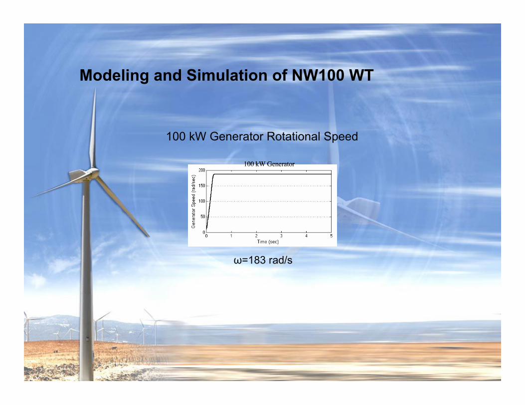
Table: Electrical Characteristics of NW100 Wind Turbines
Table: Electrical Characteristics of 925 kW Diesel Generators
Table: Electrical Characteristics of 250 kW Hydrogen Generators
Electrical Performance of System Components (cont.)
Table: Electrical Characteristics of the Whole System
Figure: Monthly Energy Production by Wind, Diesel and Hydrogen
Electrical Performance of System Components (cont.)
Electrical Performance of System Components
Figure: Excess Electricity and Unmet Load of Ramea Hybrid Power System
! Excess energy – 259,549 kWh per year.
! Unmet load – 302 kWh per year.
! Capacity shortage – 704 kWh
WECS Components
! Rotor Blades
! Shaft and Bearings
! Brakes
! Electrical Generator
! Transformer
! Capacitor Bank
Mechanical
Drive Unit
Generator
Switching and
Protective
Equipment
Transformer, Power
Lines, Mains
Consumers,
StorageControl and
Supervision
Mechanical EnergyKinetic
Energy
Rotor
Blades
Electrical Energy
Wind Energy
Conversion
Torque and Speed
Conversion
Mechanical to
Electrical Energy
Conversion
Wind
Power Extraction from the Wind
( ) 3,2
1wpt vACP !"#=
( ) !"!
"! !643
1
2
11
5
, ceccc
cC
c
p +##$
%&&'
())=
)
1
035.0
08.0
11
3
1+
!+
=""##
wv
R!" =
( )( ) 22,
2
1,
2
1wqw
p
t vARCvC
ART !"#"
!"# ==
( )( )!
"!"!
,,
p
q
CC =
Modeling and Simulation of WM15S WT (cont.)
vw=5 m/sv
w=5 m/s v
w=6 m/sv
w=6 m/s v
w=7 m/sv
w=7 m/s
13 kW Generator in Operation
0.25 kW Output 1.48 kW Output 3.05 kW Output
Modeling and Simulation of WM15S WT (cont.)
65 kW Generator in Operation
vw=8 m/sv
w=8 m/s v
w=9 m/sv
w=9 m/s
vw=10 m/sv
w=10 m/s
vw=11 m/sv
w=11 m/s
24 kW Output 32.9 kW Output
41.4 kW Output 48.9 kW Output
Modeling and Simulation of WM15S WT (cont.)
65 kW Generator in Operation
vw=12 m/sv
w=12 m/s
55.3 kW Output 60.2 kW Output
63.7 kW Output 65.8 kW Output
vw=13 m/sv
w=13 m/s
vw=14 m/sv
w=14 m/s v
w=15 m/sv
w=15 m/s
Modeling and Simulation of WM15S WT
Generator Rotational Speeds
13 kW Generator13 kW Generator 65 kW Generator65 kW Generator
!1=128 rad/s !2=125 rad/s
Modeling and Simulation of NW100 WT (cont.)
vw=5 m/sv
w=5 m/s v
w=6 m/sv
w=6 m/s v
w=7 m/sv
w=7 m/s
2.8 kW Output 14.1 kW Output 29.2 kW Output
46 kW Output 62.3 kW Output 76.1 kW Output
vw=8 m/sv
w=8 m/s v
w=9 m/sv
w=9 m/s v
w=10 m/sv
w=10 m/s
Modeling and Simulation of NW100 WT (cont.)
vw=11 m/sv
w=11 m/s
86.6 kW Output 93.4 kW Output 97.1 kW Output
vw=12 m/sv
w=12 m/s v
w=13 m/sv
w=13 m/s
vw=14 m/sv
w=14 m/s v
w=15 m/sv
w=15 m/s
98.2 kW Output 98.2 kW Output
Modeling and Simulation of NW100 WT
100 kW Generator100 kW Generator
100 kW Generator Rotational Speed
!=183 rad/s
Comparison of Actual and Simulated Power Curves
Larger Generator Operating Region
Smaller Generator
Operating Region
Larger Generator Operating RegionLarger Generator Operating Region
Smaller Generator
Operating Region
Smaller Generator
Operating Region
Power Curves of WM15S WT Power Curves of NW100 WT
Modeling of Alkaline type Electrolyzer (cont.)
Cathode
(Ni, C -Pt)
2e-
2e-
+-
H2
_ O2
H2O H
2O
2OH - 2OH-
Anode
(Ni, Co, Fe)
Diaphragm
(NiO)
Electrolyte
(30% wt. KOH)
Cathode
(Ni, C -Pt)
2e-
2e-
+-
H2
_ O2
H2O H
2O
2OH - 2OH-
Anode
(Ni, Co, Fe)
Diaphragm
(NiO)
Electrolyte
(30% wt. KOH)
Figure: Internal structure of analkaline electrolyzer.
! 30% KOH is added toincrease the conductivity level ofthe electrolyte.
! Anode made of Ni, Co & Feand Cathode made of Ni & C-Ptprevent corrosion and ensuregood conductivity.
! For the same reasondiaphragm is made up of NiO.
Modeling of Alkaline type Electrolyzer (cont.)
! H2 flow rate
! Cell voltage
! Faraday efficiency
! Energy efficiency
Figure: Electrochemical Model.
Modeling of Alkaline type Electrolyzer
Figure: Thermal Model.
! Heat generation
! Heat loss
! Cooling demand
! Temperature
Simulations of Alkaline type Electrolyzer (cont.)
Figure: Current & Power. Figure: H2 Generation. Figure: Faraday &Energy Efficiencies.
Figure: Cell Voltage.
Simulations of Alkaline type Electrolyzer
Figure: Heat Generation. Figure: Heat Loss. Figure: Auxiliary Cooling.
Figure: Temperature.
Modeling of H2 Tanks
Figure: SimulinkModel of H2 Tank.
Figure: Three Hydrogen Tanks of 1000 Nm3
combined Capacity .
Modeling of H2 Engines
Figure: Simulink Model of H2 Engines.
! Throttle body dynamics
! Manifold dynamics
! Rotational dynamics
Simulations of H2 Engines
Figure: H2 Flow Input to Engines. Figure: Mech. Power from Engines.
Figure: Synchronous Speed of the Engines.
Simulations of H2 Generator
25.626.420.550
32.633.630.700
39.640.830.850
46.548.001.000
53.555.251.150
60.562.501.300
68.570.701.472
Electrical PowerHydrogen
Generator (kW)
Mechanical Powerfrom Hydrogen
Engine (kW)
Tank OutputFlow Rate
(mol/s)
Figure: H2 Generator Output Power.
CS1: Simulation with Variable Load (1200/1600/1200 kW)
! Wind speed – 15 m/s.
! Dump load increases to minimizethe effect of the main load declination.
! Secondary load current – 0.8 pu.
CS2: Simulation with Variable Wind Speed (15/10/15 m/s)
! Main load – 1200 kW.
! WTs respond to the wind speedchange accordingly.
! In the second stage the additionalload is met by diesel generator.
! SL has to increase as to minimize theeffect of high wind generation.
! Secondary load current – 0.5 pu.
CS2: Simulation with Variable Wind Speed (7/8 m/s)
! Main load – 500 kW.
! WTs respond to the wind speedchange accordingly.
! In the second stage the diesel poweris reduced.
! SL has to increase as to minimize theeffect of high wind generation.
! Secondary load current – 0.5 pu.
CS2: Simulation with Variable Wind Speed (12/13 m/s)
! Main load – 300 kW.
! WTs respond to the wind speedchange accordingly.
! In the second stage the diesel poweris reduced.
! SL has reached to its rated value.
! Secondary load current – 1 pu.
CS3: Simulation with Electrolyzer in Operation (cont.)
Figure: Current and Power. Figure: H2 Production.
Figure: Faraday Efficiency and Temperature.
! Electrolyzer current – 160A.
! Electrolyzer power – 45 kW.
! H2 production rate – 4.6 Nm3/hr.
! Faraday efficiency – 78%.
CS3: Simulation with Electrolyzer in OperationD
iese
l P
ow
er (
kW
)D
iese
l P
ow
er (
kW
)
! Main load – 1200 kW.
! WTs and diesel generator areoperating at rated conditions.
! Secondary load – 400 kW.
CS4: Simulation with HG in Operation
Engin
e P
ow
er (
W)
Engin
e P
ow
er (
W)
! Main load – 200 kW.
! WTs are operating below cut-in wind speed.
! Secondary load – 60 kW.
! Both diesel and H2 gensets are producing130 kW individually.
CS5: Simulation with DG in Operation
! Main load – 500/700/500 kW.
! No wind generation
! No H2 generation
! Diesel generation follows the load.
! SL increases to 200 kW.
! SL current – 0.5 pu.
Hydrogen Storage Dynamics
! 10-20 sec: Electrolyzer in operation.
! 20-25 sec: Both electrolyzer and H2
generators are non-operating.
! 25-27 sec: H2 generators in operation.
Conclusions
! Dynamic model of Wind-Diesel-Hydrogen basedRamea power system has been developed.
! Hydrogen as a storage medium is a novelapproach adopted in this system.
! Introducing of new WECS is aiming at increasingthe penetration level.
! The dump load used in this system played animportant role in maintaining stability.
Future Works
! Introduce precise control mechanisms.
! Flywheel and pumped hydro as alternative storagesystems.
! Design stand-alone energy systems for other remotecommunities.
! Energy consumed by the SL might be used for waterheating, room heating, water pumping etc.