36
College of Engineering K T C ENTUCKY RANSPORTATION ENTER GROUND PENETRATING RADAR “PAVEMENT LAYER THICKNESS EVALUATION” Research Report KTC-02-29/FR101-00-1F UNIVERSITY OF KENTUCKY

College of Engineering
KT
C
ENTUCKY
RANSPORTATION
ENTER
GROUND PENETRATING RADAR“PAVEMENT LAYER THICKNESS EVALUATION”
Research ReportKTC-02-29/FR101-00-1F
UNIVERSITY OF KENTUCKY

For more information or a complete publication list, contact us at:
KENTUCKY TRANSPORTATION CENTER176 Raymond BuildingUniversity of Kentucky
Lexington, Kentucky 40506-0281
(859) 257-4513(859) 257-1815 (FAX)
1-800-432-0719www.engr.uky.edu/ktc
The University of Kentucky is an Equal Opportunity Organization
We provide services to the transportation communitythrough research, technology transfer and education.We create and participate in partnerships to promote
safe and effective transportation systems.
Our Mission
We Value...Teamwork -- Listening and Communicating, Along with Courtesy and Respect for Others
Honesty and Ethical BehaviorDelivering the Highest Quality Products and Services
Continuous Improvement in All That We Do

Research Report
KTC-02-29/FR101-00-1F
GROUND PENETRATING RADAR “PAVEMENT LAYER THICKNESS EVALUATION”
by
David A. Willett Assoc. Research Engineer
and Brad Rister
Research Engineer
Kentucky Transportation Center College of Engineering University of Kentucky Lexington, Kentucky
in cooperation with
Kentucky Transportation Cabinet
Commonwealth of Kentucky
The contents of this report reflect the views of the authors who are responsible for the facts and accuracy of the data presented
herein. The contents do not necessarily reflect the official views or policies of the University of Kentucky or the Kentucky Transportation
Cabinet. This report does not constitute a standard, specification, or regulation. The inclusion of manufacturer names and trade names is for
identification purposes and is not to be considered an endorsement.
December 2002

TABLE OF CONTENTS
EXECUTIVE SUMMARY .................................................................................................1
1.0 INTRODUCTION ...................................................................................................2
2.0 OBJECTIVE ............................................................................................................2
3.0 G.P.R. Background “How it works for pavement thickness evaluation” ................3
4.0 Performance Tests....................................................................................................5
4.1 Signal to Noise Ratio Test ...........................................................................5
4.2 End Reflection Test......................................................................................6
4.3 Signal Stability Test.....................................................................................6
4.4 Concrete Penetration Test ............................................................................7
5.0 Data and Results ......................................................................................................7
5.1 University of Kentucky Campus Parking Lot..............................................9
5.1.1 G.P.R. Repeatability ........................................................................9
5.1.2 Significance of Applying Ground Truth to Processed Data ..........10
5.1.3 Effects of Surface Water on G.P.R. ...............................................11
5.2 Interstate-75 ...............................................................................................13
5.3 Interstate-64 ...............................................................................................14
5.4 Kentucky 17 ...............................................................................................15
5.5 US 27 (Paris Pike)......................................................................................17
5.6 Interstate-275 .............................................................................................18
5.6.1 Interstate-275EBLLA ....................................................................18
5.6.2 Interstate-275EBLL2 .....................................................................19
5.6.3 Interstate-275EBLLB.....................................................................20
5.6.4 Interstate-275WBLL1....................................................................21
5.6.5 Interstaet-275WBLLA ...................................................................22
6.0 Summary of Data and Results................................................................................23
7.0 Pavement Layer Thickness Results from Other Research Institutions..................26
7.1 Texas Transportation Institute ...................................................................26
7.2 Infrasense Inc. ............................................................................................26
7.3 Florida DOT State Project 99700-7550 .....................................................26
8.0 Federal Communication Commission (FCC) ........................................................27
9.0 SUGGESTIONS ....................................................................................................27
10.0 CONCLUSIONS....................................................................................................28
APPENDIX A: Radan “Step-by-Step Post Processing Process” ............................29
REFERENCES: .................................................................................................................30
LIST OF TABLES
Table 1. Dielectric Constants .....................................................................................3
Table 2. Parking lot repeatability ground truth averages .........................................10
Table 3. Parking lot ground truth averages ..............................................................11
Table 4. Parking lot dry, wet/dry, wet averages.......................................................13
Table 5 . Interstate-75 ground truth averages ...........................................................14
Table 6. Interstate-64 ground truth averages ...........................................................15
Table 7. KY17 ground truth averages......................................................................16
Table 8 . Paris Pike ground truth averages................................................................17
Table 9. Concrete allowances/pay scales.................................................................18
Table 10. Interstate-275EBLLA ground truth averages.............................................19
Table 11. Interstate-275EBLL2 ground truth averages .............................................20
Table 12. Interstate-275EBLLB ground truth averages.............................................21
Table 13. Interstate-275WBLL1 ground truth averages ............................................22
Table 14. Interstate-275WBLLA ground truth averages ...........................................23
Table 15 . Summarized GPR Thickness Data.............................................................24
LIST OF FIGURES
Figure 1. Performance test waveform .........................................................................6
Figure 2. Calibration picture .......................................................................................8
Figure 3. Ground Truth demonstration graph .............................................................9
Figure 4. Parking lot repeatability graph...................................................................10
Figure 5. Parking lot ground truth graph...................................................................11
Figure 6. Parking lot wet surface picture ..................................................................13
Figure 7. Parking lot dry, half wet/half dry, wet graph .............................................14
Figure 8. Interstate-75 ground truth graph ................................................................14
Figure 9. Interstate-64 ground truth graph ................................................................15
LIST OF FIGURES
Figure 10. KY 17 ground truth graph..........................................................................16
Figure 11. Paris Pike ground truth graph ....................................................................17
Figure 12. Interstate-275EBLLA ground truth graph .................................................19
Figure 13. Interstate-275EBLL2 ground truth graph ..................................................20
Figure 14. Interstate-275EBLLB ground truth graph..................................................21
Figure 15. Interstate-275WBLL1 ground truth graph .................................................22
Figure 16. Interstate-275WBLLA ground truth graph ................................................23
Figure 17. Asphalt – Ground Truth Summary ............................................................25
Figure 18. Concrete – Ground Truth Summary ..........................................................25

1
Executive Summary
The following report demonstrates the accuracy of using Ground Penetrating Radar (GPR) to determine both the surface layer thickness for asphalt, and concrete pavements. In addition tests were conducted to identify GPR’s repeatability on dry pavements, GPR’s ability to determine pavement layer thicknesses in wet conditions, and an attempt was made to determine the number of actual field cores necessary to accurately post-process radar data into thickness values.
The equipment used to perform these evaluations was Geophysical Survey Systems Inc.’s model SIR 10B with the model 4108 (1 GHz.) air-launched horn antenna.
Preliminary results indicate that when ground truth cores were used, GPR calculated thicknesses varied from actual core thicknesses by:
• Asphalt less than two inches:
o +/-10.32% to +/-0.40% o +/-0.20 to +/-0.01 inches
• Asphalt bases of eight to nine inches: o +/-2.73% to +/-1.34% o +/-0.24 to +/-0.12 inches
• Concrete nine to twelve inches: o +/-14.24 to +/-0.05% o +/-1.66 to +/-0.01 inches
The results from the additional test mentioned above may be found inside this
report.

2
1. 0 Introduction Currently in Kentucky, both asphalt and concrete paving surfaces are cored approximately every 1000 linear feet to check for specification compliance according to Kentucky Method 64-420-95, 64-309-95 respectively. The allowable tolerance for asphalt paving is plus/minus 0.5 inches and plus/minus 0.2 inches for concrete. Although coring of both materials has been a standard means of determining pavement layer thickness in Kentucky for many years, recently developed Ground Penetrating Radar equipment has been used with some success in both Texas and Florida as a means of determining pavement layer thicknesses in a non-destructive environment. In addition, G.P.R. has also been proven to collect continuous pavement layer thicknesses at highway speeds.1 In hopes of further understanding the possibilities of using G.P.R. to determine thicknesses of pavement surface layers, the Kentucky Transportation Center has evaluated the SIR 10B G.P.R. system manufactured by Geophysical Survey Systems Inc. (G.S.S.I.). Thickness comparisons have been made between actual core thicknesses and the calculated thicknesses obtained from the G.P.R. equipment. The test sections that were used to evaluate the equipment/technology are as follows: four asphalt sections, three non-reinforced Portland cement concrete pavement (PCCP) sections, and one asphalt parking lot surface. 2.0 Objective
The objective of this study was to determine the accuracy of G.P.R. for determining pavement surface thicknesses. In addition, several other tests were conducted to identify GPR’s repeatability on dry pavements, GPR’s ability to determine pavement layer thicknesses in wet conditions, and an attempt was made to determine the number of actual field cores one would need to accurately post-process radar data into thickness values.
In order to evaluate GSSI’s G.P.R. pavement layer thickness accuracy, measured core values were compared from four different asphalt sections, three different concrete (PCCP) sections, and one parking lot to the output data from GSSI’s software package “Radan”. The following list identifies the sections tested during this study with its surface layer composition and mile point location.
1. Parking lot U.K. campus Asphalt 2. Interstate I-75 Asphalt 81.481-83.600 3. Interstate I-64 Asphalt 84.800-82.196 4. KY-17 Asphalt 14.809-13.025 5. Paris Pike Asphalt 0.400-2.379 6. Interstate I-275 east Concrete 7.670-5.882 7. Interstate I-275 east Concrete 3.716-2.000 8. Interstate I-275 west Concrete 2.000-3.944
The radar data obtained from the projects listed above were evaluated by using the two techniques listed below to determine the pavement layer thicknesses. Thickness

3
results from these test sections will be displayed in the section titled “Data and Results” later in this report.
1. No applied core values or what will be referred to as “no ground truth” later in this report. No applied core values simply means that processed radar data was compared to actual known pavement layer thicknesses without any post-processing adjustment.
2. Multiple core values or what will be referred to as “ground truth” later in this report: Multiple known core values simply means that processed radar data was compared to actual known pavement layer thicknesses with an applied adjustment factor. A further explanation of “ground truth” and its application will be given in the section titled “Data and Results”.
3.0 G.P.R. Background “How it works for pavement thickness evaluation”
Although it is not the intent of this study to fully discuss the theoretics behind how G.P.R. technology works, this section will give a brief overview of G.P.R. basics and the associated equations needed to calculate pavement layer thicknesses. For a more detailed explanation of the theoretics behind G.P.R. technology please refer to the reports titled “Development of a Procedure for the Automated Collection of Flexible Pavement Layer Thicknesses and Materials: Phase I: Demonstration of Existing Ground Penetrating Radar Technology”, and “Implementation of the Texas Ground Penetrating Radar System” both written by the Texas Transportation Institute.2&3
Ground Penetrating Radar is a series of electromagnetic pulses transmitted into the pavement surface by either an air-launched horn or ground coupled antenna. The transmitted pulses are reflected back to the antenna showing the pavement properties by measuring the amplitude and arrival time of the pulse. The change in the amplitude and arrival time of the pulse has a direct relationship to the change of the electrical properties of the pavement. The change of the electrical properties of the material is referred to as the change in dielectric constant.
As seen below, in Table 1, different highway related building materials have different dielectric constants. It should be noted, that the dielectric property of any given material is crucial to radar evaluations. Without the change in dielectric constant between materials, radar technology would not be able to determine the interface between different layers.4 Table 1: Dielectric Constants
Material
Dielectric Constant
Air 1 Water 81
Asphalt 3 to 6 Concrete 6 to 11
Limestone 4 to 8 Clays 5 to 40
Dry Sand 3 to 5 Saturated Sand 20 to 30
4
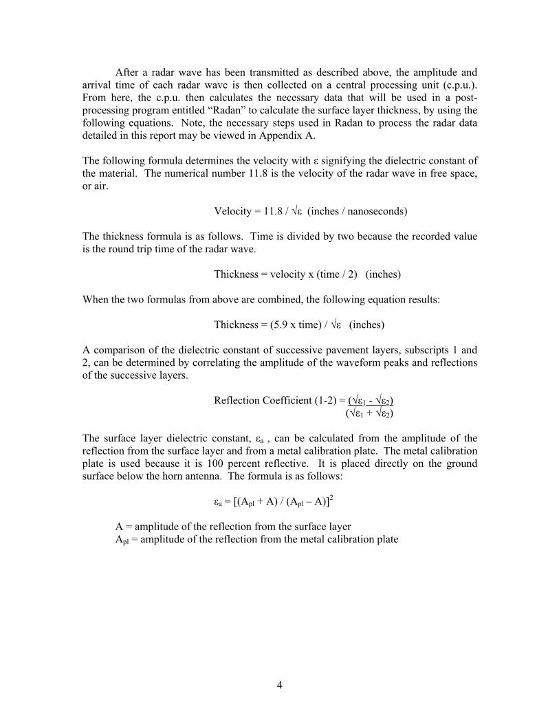
After a radar wave has been transmitted as described above, the amplitude and arrival time of each radar wave is then collected on a central processing unit (c.p.u.). From here, the c.p.u. then calculates the necessary data that will be used in a post-processing program entitled “Radan” to calculate the surface layer thickness, by using the following equations. Note, the necessary steps used in Radan to process the radar data detailed in this report may be viewed in Appendix A.
The following formula determines the velocity with ε signifying the dielectric constant of the material. The numerical number 11.8 is the velocity of the radar wave in free space, or air.
Velocity = 11.8 / √ε (inches / nanoseconds) The thickness formula is as follows. Time is divided by two because the recorded value is the round trip time of the radar wave.
Thickness = velocity x (time / 2) (inches) When the two formulas from above are combined, the following equation results:
Thickness = (5.9 x time) / √ε (inches) A comparison of the dielectric constant of successive pavement layers, subscripts 1 and 2, can be determined by correlating the amplitude of the waveform peaks and reflections of the successive layers.
Reflection Coefficient (1-2) = (√ε1 - √ε2) (√ε1 + √ε2) The surface layer dielectric constant, εa , can be calculated from the amplitude of the reflection from the surface layer and from a metal calibration plate. The metal calibration plate is used because it is 100 percent reflective. It is placed directly on the ground surface below the horn antenna. The formula is as follows:
εa = [(Apl + A) / (Apl – A)]2
A = amplitude of the reflection from the surface layer Apl = amplitude of the reflection from the metal calibration plate

5
The calculation of the dielectric constant of subsequent layers, namely the base layer, εb, can be calculated in a similar fashion.
εb = εa [(F - R2) / (F + R2)]2 where: F = 4√εa
(1 – εa)
R2 = ratio of the reflected amplitude from the top of the base layer to the top of the surface layer.
4.0 Performance Tests In order to properly conduct automated signal processing using G.P.R. equipment, the Texas Transportation Institute has devised the following performance tests that may be performed before purchasing G.P.R. equipment.3 These tests are conducted to ensure that the quality of the G.P.R. waveforms are of a sufficient level. Please note that all performance test results below have been performed using GSSI’s Sir 10B G.P.R. system with a 1.0 GHz. air-launched horn antenna. In addition, the horn-antenna is mounted approximately 18-20 inches above ground level.
4.1 Signal to Noise Ratio Test The Signal to Noise Ratio Test tests the amount of clutter or noise that is in the equipment otherwise known as systematic error. The following signal to noise ratio formula and the results from G.S.S.I.’s Sir 10B system may be viewed below.
Noise Level < 5% Signal Level
Noise Level is the maximum amplitude of a peak that is between 2 and 10 ns after the metal plate reflection (see Figure 1). Signal Level is the reflection metal plate amplitude measured from the peak to the preceding minimum (see Figure 1).
Results from G.S.S.I.’s Sir 10B: 1038 / 28665 = 3.6% < 5% OK

6
Figure 1: Performance test waveform
4.2 End Reflection Test
The End Reflection Test uses the same setup configurations and data as the Signal to Noise Ratio Test. It measures the amplitude of the end reflection preceding the metal plate reflection. The following end reflection formula and the results from G.S.S.I.’s Sir 10B system may be viewed below.
AE < 50% Signal Level
AE is the amplitude of the end reflection located in the 4 nanosecond area preceding the surface echo (see Figure 1).
Results from GSSI’s Sir 10B: 2242 / 28665 = 7.8% < 50% OK
4.3 Signal Stability Test The Signal Stability Test uses the same setup as the Signal to Noise Ratio Test with a minimum of 50 recorded waveforms and no less than 25 waveforms/second. The following signal stability formula and the results from G.S.S.I.’s Sir 10B system may be viewed below.
Amax – Amin < 1% Aavg

7
Amax, Amin, and Aavg are the maximum, minimum and average of the amplitude for any of the recorded wavelengths.
Results from G.S.S.I.’s Sir 10B: (19468-19148) / 19297.12 = 1.6583% TOO HIGH As it can be seen from the above calculation, the G.S.S.I. Sir 10B system performed slightly higher than the requirements outlined by the Texas Transportation Institute for the signal stability test.
4.4 Concrete Penetration Test The Concrete Penetration Test is performed using a 6 inch thick, 36 inch by 36 inch non-reinforced concrete slab placed over a metal plate. The minimum cure date for the concrete specimen is 28 days. However, a longer cure time may be needed in order to pass the test’s recommendations. The following concrete penetration formula and the results from G.S.S.I.’s Sir 10B system may be viewed below.
Abottom > 25% Atop
Abottom is defined as the amplitude of reflection from the metal plate beneath the concrete. Atop is defined as the amplitude of reflection from the surface.
Results from G.S.S.I.’s Sir 10B: 1 month cure time 15.74% (too low) 3 month cure time 41.898% (pass) 5.0 Data and Results
For the study and evaluation of G.P.R.’s ability to accurately determine pavement surface layer thicknesses, several projects were evaluated across the state of Kentucky. The following is a list of these projects:
1. Parking lot U.K. campus Asphalt 2. Interstate I-75 Asphalt 81.481-83.600 3. Interstate I-64 Asphalt 84.800-82.196 4. KY-17 Asphalt 14.809-13.025 5. Paris Pike Asphalt 0.400-2.379 6. Interstate I-275 east Concrete 7.670-5.822 7. Interstate I-275 east Concrete 3.716-2.000 8. Interstate I-275 west Concrete 2.000-3.944
However, before radar data can be processed into thickness readings in Radan, a
calibration file must first be recorded for each project. The calibration file is recorded by laying a 4x4 foot metal plate underneath the air launched horn antenna, and having a

8
couple of people jump up and down on the back bumper of the radar truck (Figure 2). This file is used to help simulate how much the truck may bounce if it encounters bumps while the data is being collected. After this file has been collected and recorded, it is then incorporated into each recorded project file during post processing. It should be noted that the calibration file should be comprised of approximately two-hundred scans.
Figure 2: Picture showing the metal plate underneath the air-launched horn before the calibration file is recorded.
In addition to using the above mentioned calibration file in the radar data post processing phase, it is also beneficial to incorporate actual measured core values, also known as ground truth, into the processed data. Ground truth is a term used to describe the way that radar data is adjusted depending on the use of cores. In comparison, zero-core value/no ground truth processed data is known as data without any post-processing adjustment. However, when you apply ground truth, a known core value and its location is typed in while processing the radar data in Radan. The Radan software then adjusts the thicknesses for the raw radar data to correspond with the actual measured core value at the prescribed location. Radan will allow for multiple core values and their respective locations to be typed in for ground truth points. However it should be noted that when more than one ground truth point is used, the data is shifted and adjusted at the midway point between two cores (Figure 3).

9
Figure 3: Ground Truth demonstration graph
5.1 University of Kentucky Campus Parking Lot
The parking lot at the University of Kentucky was used to test the repeatability of the ground penetrating radar, demonstrate the significance of applying ground truth to processed data, and to experiment with the effects that surface water has on ground penetrating radar. Note: For the remainder of this section, short colored horizontal lines have been placed on the right side of each of the graphs. These lines indicate the average value from the associated collected data. In addition, cores are numbered from left to right beginning with #1 on graphs that contain multiple actual core values.
5.1.1 G.P.R. Repeatability In order to determine if GPR was accurate, it also made sense to determine if GPR
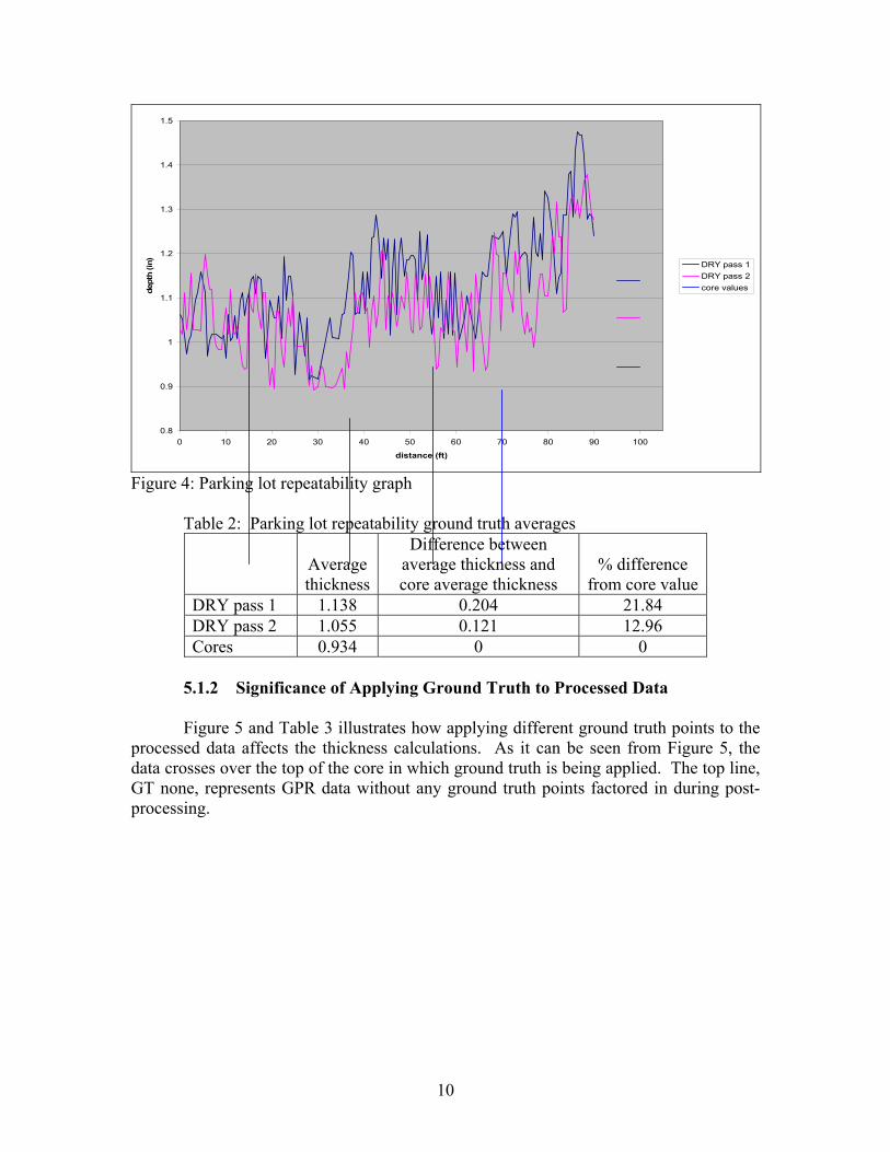
results were repeatable. Figure 4 shows a graphical representation of a G.P.R. repeatability test conducted on the surface layer of a dry one-inch pavement. This test consisted of comparing G.P.R. data from two identical passes with applied ground truth to core # 1. As it can be seen from Figure 4 and Table 2, the difference between GPR calculated thickness averages of the multiple passes is less than 0.1 inches
10
0.8
0.9
1
1.1
1.2
1.3
1.4
1.5
0 10 20 30 40 50 60 70 80 90 100
distance (ft)
dept
h (in
)
DRY pass 1DRY pass 2core values
Figure 4: Parking lot repeatability graph
Table 2: Parking lot repeatability ground truth averages
Average thickness
Difference between average thickness and core average thickness
% difference
from core value DRY pass 1 1.138 0.204 21.84 DRY pass 2 1.055 0.121 12.96 Cores 0.934 0 0
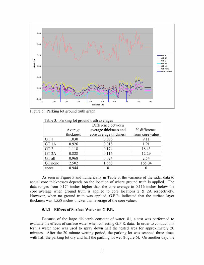
5.1.2 Significance of Applying Ground Truth to Processed Data Figure 5 and Table 3 illustrates how applying different ground truth points to the
processed data affects the thickness calculations. As it can be seen from Figure 5, the data crosses over the top of the core in which ground truth is being applied. The top line, GT none, represents GPR data without any ground truth points factored in during post-processing.
11
0.60
1.00
1.40
1.80
2.20
2.60
3.00
0 10 20 30 40 50 60 70 80 90
distance (ft)
dept
h (in
)
GT 1GT 1AGT 2GT 2AGT allGT nonecore values
Figure 5: Parking lot ground truth graph Table 3: Parking lot ground truth averages
Average thickness
Difference between average thickness and core average thickness
% difference
from core value GT 1 1.030 0.086 9.11 GT 1A 0.926 0.018 1.91 GT 2 1.118 0.174 18.43 GT 2A 0.828 0.116 12.29 GT all 0.968 0.024 2.54 GT none 2.502 1.558 165.04 cores 0.944 0 0
As seen in Figure 5 and numerically in Table 3, the variance of the radar data to
actual core thicknesses depends on the location of where ground truth is applied. The data ranges from 0.174 inches higher than the core average to 0.116 inches below the core average when ground truth is applied to core locations 2 & 2A respectively. However, when no ground truth was applied, G.P.R. indicated that the surface layer thickness was 1.558 inches thicker than average of the core values.
5.1.3 Effects of Surface Water on G.P.R. Because of the large dielectric constant of water, 81, a test was performed to
evaluate the effects of surface water when collecting G.P.R. data. In order to conduct this test, a water hose was used to spray down half the tested area for approximately 20 minutes. After the 20 minute wetting period, the parking lot was scanned three times with half the parking lot dry and half the parking lot wet (Figure 6). On another day, the

12
whole parking lot was sprayed down for approximately 20 minutes and was scanned twice. Note, only the surface of the asphalt was wet, the pavement layer was not fully saturated. Figure 7 and Table 4 demonstrates the average of the scans for the dry, half wet/half dry, and the completely wet parking lot.
Figure 6: Collecting radar data on a wet surface in the University of Kentucky campus parking lot.
0.8
0.9
1.0
1.1
1.2
1.3
1.4
1.5
0.0 10.0 20.0 30.0 40.0 50.0 60.0 70.0 80.0 90.0 100.0
distance (ft)
dept
h (in
) DRY
HALF
WET
corevalues
Figure 7: Parking lot dry, half wet/half dry, wet graph

13
Table 4: Parking lot dry, wet/dry, wet averages.
Average thickness
Difference between average thickness and core average thickness
% difference
from core value DRY 1.097 0.163 17.45 HALF 1.145 0.211 22.59 WET 1.100 0.166 17.77 Cores 0.934 0 0
As seen above in Figure 7 and Table 4, it appears that surface water has very little
effect on determining pavement layer thicknesses using G.P.R., despite the fact that water has a dielectric of 81 and asphalt has a dielectric range between 3 and 6.3 Numerically, the difference between the dry and half wet/half dry pass is 0.048 inches, and 0.003 inches between the dry and wet pass. In relation to the average of the actual core thicknesses, the half wet/half dry pass had a maximum difference of 0.211 inches. It is speculated that unless water is standing on the surface or the pavement structure or is fully saturated, the presence of water is not going to have an adverse effect on the accuracy of collecting G.P.R. data. 5.2 Interstate-75 (81.481-83.600)
Interstate-75, between mile points 81.481and 83.600, was used as a test site to evaluate the accuracy of ground penetrating radar for determining asphalt surface layer thicknesses. The asphalt design for this section on I-75 was a 1.5 inch overlay over an existing asphalt surface. Figure 8 demonstrates the calculated thicknesses using one, two, three, and zero ground truth points. The long vertical black box located in the center of the graph represents an area of possible interference as the radar truck passed by trucks, rollers, and graders.
Since the asphalt design was for a 1.5 inch overlay, the contractor is allowed plus or minus a half inch from the design thickness. The two red lines on the right side of Figure 8 labeled allowance represent the range the contractor is allowed to be within. If the contractor is on the outside of the allowance on the lower end, he/she may be required to provide additional material to bring the surface layer into plan thickness.5

14
0.5
1
1.5
2
2.5
3
3.5
4
-100 1900 3900 5900 7900 9900 11900
distance (ft)
dept
h (in
)
GT 1GT 1&3&6GT 1&6GT noneallowancecore values
Figure 8: Interstate-75 ground truth graph Table 5: Interstate-75 ground truth averages
Average thickness
Difference between average thickness and core average thickness
% difference
from core value GT 1 2.277 0.319 16.29 GT 1&3&6 1.789 (0.169) 8.63 GT 1&6 2.160 0.202 10.32 GT none 2.417 0.459 23.44 Cores 1.958 0 0
The importance of using multiple ground-truth points when processing radar data
can be clearly demonstrated in Figure 8. As the number of ground truth point’s increase, the closer the lines get to the average core value. However, when no ground truth is applied the difference between the average core values and GT none is 0.459 inches.
5.3 Interstate-64 (84.800-82.196) The ground penetrating radar data collected from Interstate-64 was processed in a similar fashion as it was on I-75 above, with one, two, three, and no ground truth points. The processed radar data may be viewed in Figure 9 and Table 6. The long black vertical box shown on Figure 9 represents data that was collected while passing over a concrete bridge.

15
0.5
1
1.5
2
2.5
3
3.5
-100 1900 3900 5900 7900 9900 11900 13900
distance (ft)
dept
h (in
)
GT 1GT 1&4&7GT 1&7GT noneallowancecore values
Figure 9: Interstate-64 ground truth graph Table 6: Interstate-64 ground truth averages
Average thickness
Difference between Average thickness and core average thickness
% difference
from core value GT 1 1.000 (0.511) 33.82 GT 1&4&7 1.505 (0.006) 0.40 GT 1&7 1.377 (0.134) 8.87 GT none 1.599 (0.088) 5.82 cores 1.511 0 0
As displayed in Figure 9 and Table 6, as more ground truth points were used in
processing the radar data, the closer the average radar data was to the core average. It should be noted that the processed radar data using three cores is almost identical to the core average as it differs by 0.006 inches. However when ground truth was not applied, the difference between no-ground truth and the average core values was 0.088 inches. 5.4 KY 17 (14.809-13.025)
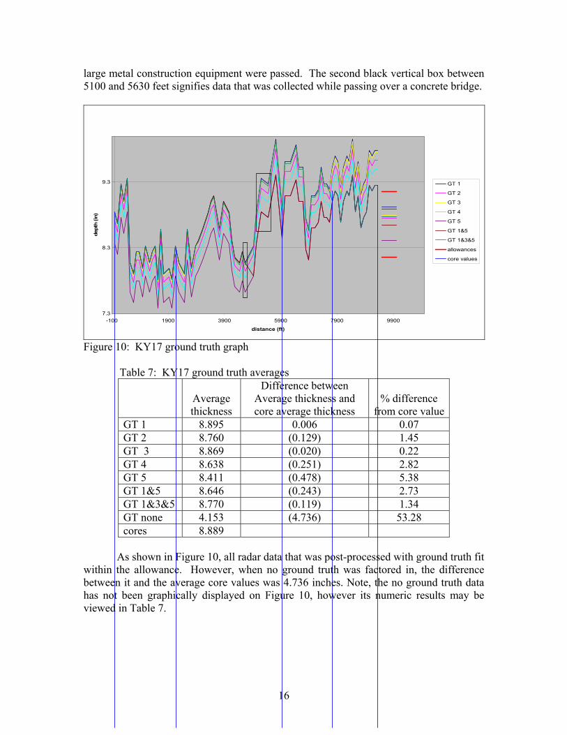
G.P.R. was used to determine the total base layer thickness before the asphalt surface was in place from mile-point 14.809 to mile-point 13.025 on KY 17. This particular test section consisted of an 8.660 inch asphalt concrete grade (PG64-22). The calculated GPR thicknesses along with the ground truth core values are graphically and numerically displayed in Figure 10 and Table 7, respectfully. It should be noted that the first black box located between 4500-4800 feet in Figure 10 is a possible location where the radar experienced outside interference. At this particular location several pieces of
16
large metal construction equipment were passed. The second black vertical box between 5100 and 5630 feet signifies data that was collected while passing over a concrete bridge.
7.3
8.3
9.3
-100 1900 3900 5900 7900 9900
distance (ft)
dept
h (in
)
GT 1
GT 2
GT 3
GT 4
GT 5
GT 1&5
GT 1&3&5
allowances
core values
Figure 10: KY17 ground truth graph Table 7: KY17 ground truth averages
Average thickness
Difference between Average thickness and core average thickness
% difference
from core value GT 1 8.895 0.006 0.07 GT 2 8.760 (0.129) 1.45 GT 3 8.869 (0.020) 0.22 GT 4 8.638 (0.251) 2.82 GT 5 8.411 (0.478) 5.38 GT 1&5 8.646 (0.243) 2.73 GT 1&3&5 8.770 (0.119) 1.34 GT none 4.153 (4.736) 53.28 cores 8.889
As shown in Figure 10, all radar data that was post-processed with ground truth fit
within the allowance. However, when no ground truth was factored in, the difference between it and the average core values was 4.736 inches. Note, the no ground truth data has not been graphically displayed on Figure 10, however its numeric results may be viewed in Table 7.

17
5. 5 US 27 (Paris Pike) (0.400-2.379)
The ground penetrating radar was used on a newly constructed section of US 27 (Paris Pike) from mile-points 0.400 to 2.379 to determine the surface layer thickness. By design, the asphalt surface was to be constructed of a 1.5-inch (PG 70-22) grade mixture. Figure 11 and Table 8 graphically and numerically depicts the processed radar data from Paris Pike.
0.75
0.95
1.15
1.35
1.55
1.75
1.95
2.15
2.35
2.55
0 2000 4000 6000 8000 10000 12000
distance (ft)
dept
h (in
)
GT 1GT 2GT 3GT 4GT 5GT 1&5GT 1&3&5allowancecore values
Figure 11: Paris Pike ground truth graph Table 8: Paris Pike ground truth averages
average
Difference between Average and core average
% difference from core value
GT 1 1.664 0.123 7.98 GT 2 2.149 0.608 39.45 GT 3 1.215 (0.326) 21.16 GT 4 1.334 (0.207) 13.43 GT 5 1.411 (0.130) 8.44 GT 1&5 1.562 0.021 1.36 GT 1&3&5 1.462 (0.079) 5.13 cores 1.541
As it can be seen from Figure 11, all of the processed radar data is located within
the allowance except for ground truth two. However, it appears that the radar data processed with the first and last ground truth points is closer to the average core values than the radar data processed with one and three ground truth cores.
18
5.6 Interstate-275
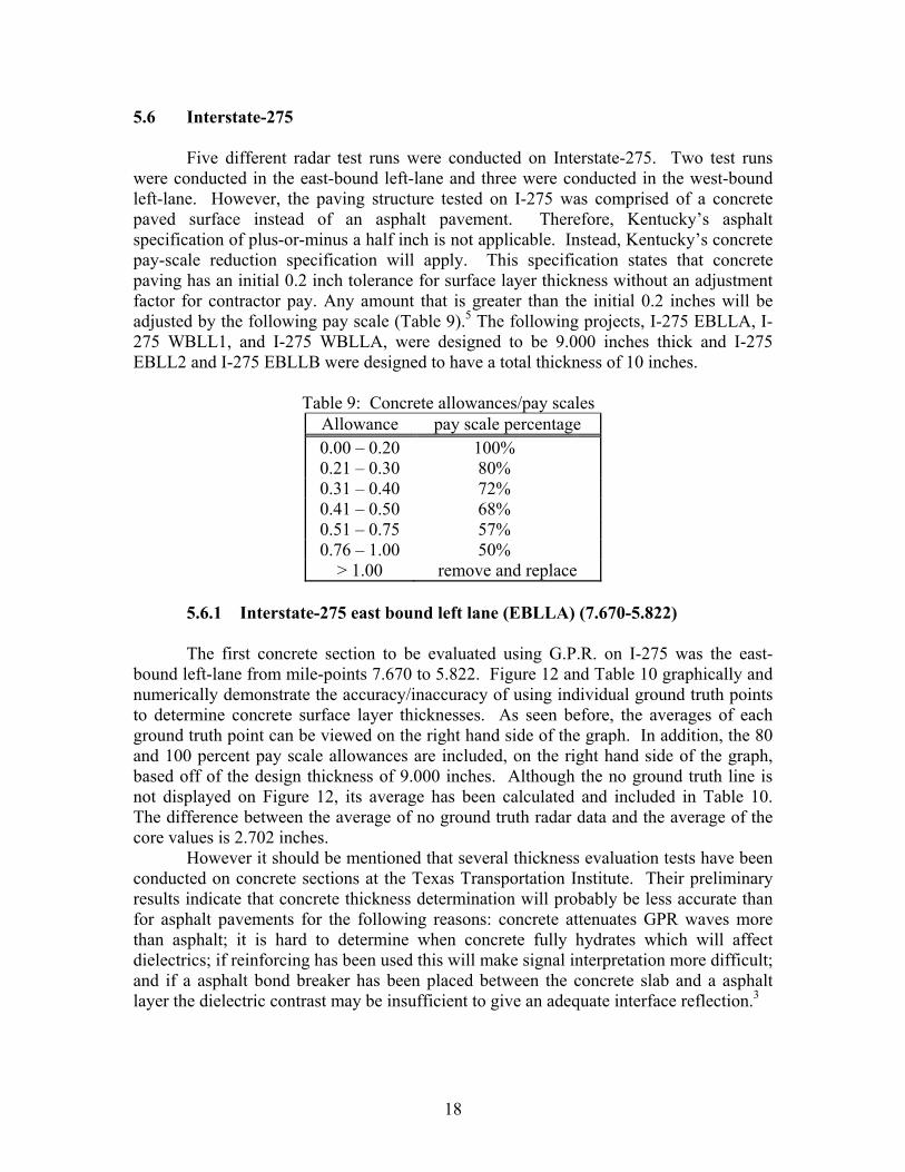
Five different radar test runs were conducted on Interstate-275. Two test runs were conducted in the east-bound left-lane and three were conducted in the west-bound left-lane. However, the paving structure tested on I-275 was comprised of a concrete paved surface instead of an asphalt pavement. Therefore, Kentucky’s asphalt specification of plus-or-minus a half inch is not applicable. Instead, Kentucky’s concrete pay-scale reduction specification will apply. This specification states that concrete paving has an initial 0.2 inch tolerance for surface layer thickness without an adjustment factor for contractor pay. Any amount that is greater than the initial 0.2 inches will be adjusted by the following pay scale (Table 9).5 The following projects, I-275 EBLLA, I-275 WBLL1, and I-275 WBLLA, were designed to be 9.000 inches thick and I-275 EBLL2 and I-275 EBLLB were designed to have a total thickness of 10 inches.
Table 9: Concrete allowances/pay scales Allowance pay scale percentage 0.00 – 0.20 100% 0.21 – 0.30 80% 0.31 – 0.40 72% 0.41 – 0.50 68% 0.51 – 0.75 57% 0.76 – 1.00 50%
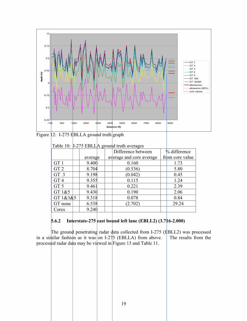
> 1.00 remove and replace 5.6.1 Interstate-275 east bound left lane (EBLLA) (7.670-5.822)
The first concrete section to be evaluated using G.P.R. on I-275 was the east-bound left-lane from mile-points 7.670 to 5.822. Figure 12 and Table 10 graphically and numerically demonstrate the accuracy/inaccuracy of using individual ground truth points to determine concrete surface layer thicknesses. As seen before, the averages of each ground truth point can be viewed on the right hand side of the graph. In addition, the 80 and 100 percent pay scale allowances are included, on the right hand side of the graph, based off of the design thickness of 9.000 inches. Although the no ground truth line is not displayed on Figure 12, its average has been calculated and included in Table 10. The difference between the average of no ground truth radar data and the average of the core values is 2.702 inches. However it should be mentioned that several thickness evaluation tests have been conducted on concrete sections at the Texas Transportation Institute. Their preliminary results indicate that concrete thickness determination will probably be less accurate than for asphalt pavements for the following reasons: concrete attenuates GPR waves more than asphalt; it is hard to determine when concrete fully hydrates which will affect dielectrics; if reinforcing has been used this will make signal interpretation more difficult; and if a asphalt bond breaker has been placed between the concrete slab and a asphalt layer the dielectric contrast may be insufficient to give an adequate interface reflection.3
19
8.25
8.5
8.75
9
9.25
9.5
9.75
10
-100 900 1900 2900 3900 4900 5900 6900 7900 8900 9900
distance (ft)
dept
h (in
)
GT 1GT 2GT 3GT 4GT 5GT 1&5GT 1&3&5allowancesallowance (80%)core values
Figure 12: I-275 EBLLA ground truth graph
Table 10: I-275 EBLLA ground truth averages
average Difference between
average and core average % difference
from core value GT 1 9.400 0.160 1.73 GT 2 8.704 (0.536) 5.80 GT 3 9.198 (0.042) 0.45 GT 4 9.355 0.115 1.24 GT 5 9.461 0.221 2.39 GT 1&5 9.430 0.190 2.06 GT 1&3&5 9.318 0.078 0.84 GT none 6.538 (2.702) 29.24 Cores 9.240
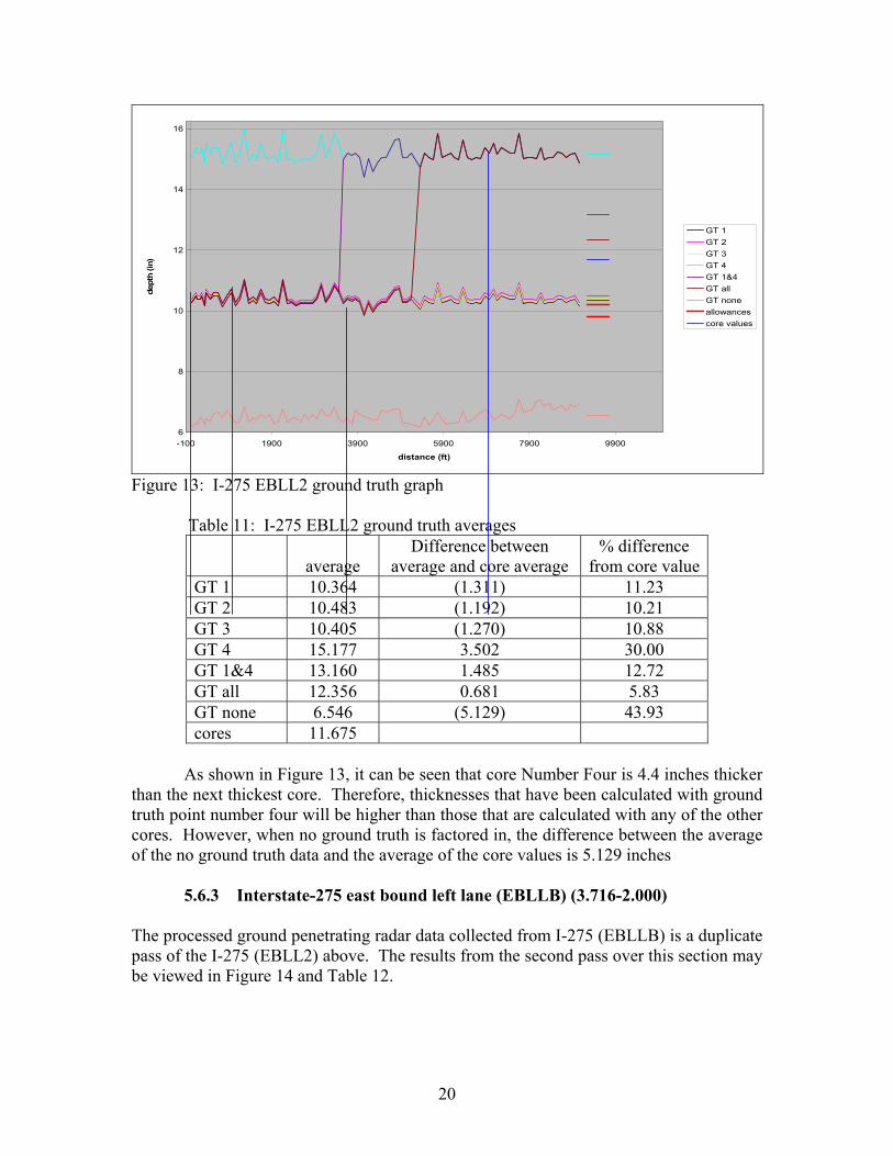
5.6.2 Interstate-275 east bound left lane (EBLL2) (3.716-2.000)
The ground penetrating radar data collected from I-275 (EBLL2) was processed
in a similar fashion as it was on I-275 (EBLLA) from above. The results from the processed radar data may be viewed in Figure 13 and Table 11.
20
6
8
10
12
14
16
-100 1900 3900 5900 7900 9900
distance (ft)
dept
h (in
)
GT 1GT 2GT 3GT 4GT 1&4GT allGT noneallowancescore values
Figure 13: I-275 EBLL2 ground truth graph Table 11: I-275 EBLL2 ground truth averages
average
Difference between average and core average
% difference from core value
GT 1 10.364 (1.311) 11.23 GT 2 10.483 (1.192) 10.21 GT 3 10.405 (1.270) 10.88 GT 4 15.177 3.502 30.00 GT 1&4 13.160 1.485 12.72 GT all 12.356 0.681 5.83 GT none 6.546 (5.129) 43.93 cores 11.675
As shown in Figure 13, it can be seen that core Number Four is 4.4 inches thicker
than the next thickest core. Therefore, thicknesses that have been calculated with ground truth point number four will be higher than those that are calculated with any of the other cores. However, when no ground truth is factored in, the difference between the average of the no ground truth data and the average of the core values is 5.129 inches
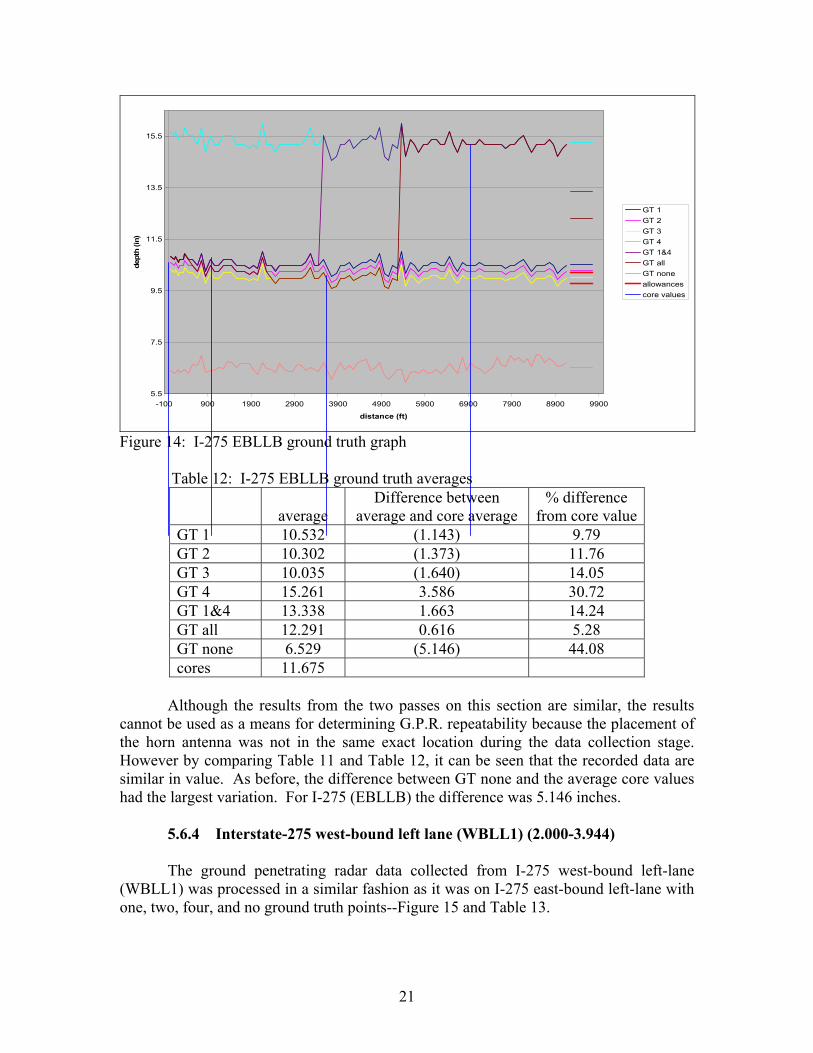
5.6.3 Interstate-275 east bound left lane (EBLLB) (3.716-2.000) The processed ground penetrating radar data collected from I-275 (EBLLB) is a duplicate pass of the I-275 (EBLL2) above. The results from the second pass over this section may be viewed in Figure 14 and Table 12.
21
5.5
7.5
9.5
11.5
13.5
15.5
-100 900 1900 2900 3900 4900 5900 6900 7900 8900 9900
distance (ft)
dept
h (in
)
GT 1GT 2GT 3GT 4GT 1&4GT allGT noneallowancescore values
Figure 14: I-275 EBLLB ground truth graph Table 12: I-275 EBLLB ground truth averages
average
Difference between average and core average
% difference from core value
GT 1 10.532 (1.143) 9.79 GT 2 10.302 (1.373) 11.76 GT 3 10.035 (1.640) 14.05 GT 4 15.261 3.586 30.72 GT 1&4 13.338 1.663 14.24 GT all 12.291 0.616 5.28 GT none 6.529 (5.146) 44.08 cores 11.675
Although the results from the two passes on this section are similar, the results
cannot be used as a means for determining G.P.R. repeatability because the placement of the horn antenna was not in the same exact location during the data collection stage. However by comparing Table 11 and Table 12, it can be seen that the recorded data are similar in value. As before, the difference between GT none and the average core values had the largest variation. For I-275 (EBLLB) the difference was 5.146 inches.
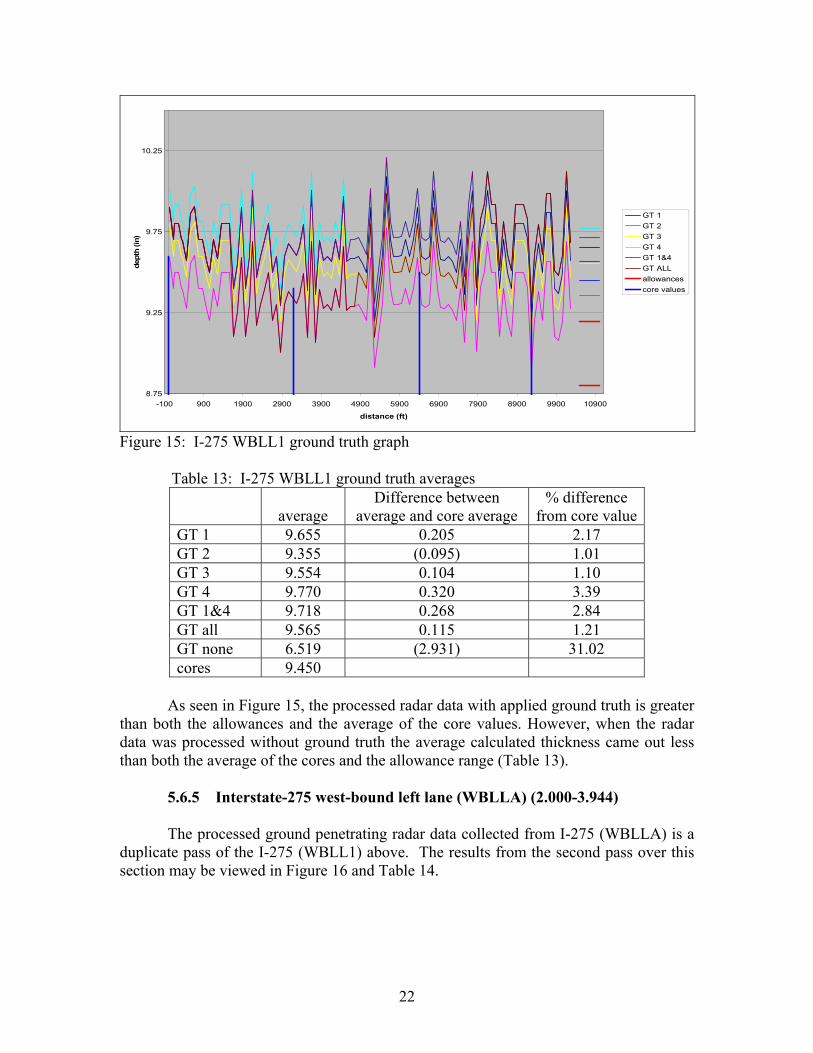
5.6.4 Interstate-275 west-bound left lane (WBLL1) (2.000-3.944)
The ground penetrating radar data collected from I-275 west-bound left-lane (WBLL1) was processed in a similar fashion as it was on I-275 east-bound left-lane with one, two, four, and no ground truth points--Figure 15 and Table 13.
22
8.75
9.25
9.75
10.25
-100 900 1900 2900 3900 4900 5900 6900 7900 8900 9900 10900
distance (ft)
dept
h (in
)
GT 1GT 2GT 3GT 4GT 1&4GT ALLallowancescore values
Figure 15: I-275 WBLL1 ground truth graph Table 13: I-275 WBLL1 ground truth averages
average
Difference between average and core average
% difference from core value
GT 1 9.655 0.205 2.17 GT 2 9.355 (0.095) 1.01 GT 3 9.554 0.104 1.10 GT 4 9.770 0.320 3.39 GT 1&4 9.718 0.268 2.84 GT all 9.565 0.115 1.21 GT none 6.519 (2.931) 31.02 cores 9.450
As seen in Figure 15, the processed radar data with applied ground truth is greater
than both the allowances and the average of the core values. However, when the radar data was processed without ground truth the average calculated thickness came out less than both the average of the cores and the allowance range (Table 13).
5.6.5 Interstate-275 west-bound left lane (WBLLA) (2.000-3.944)
The processed ground penetrating radar data collected from I-275 (WBLLA) is a duplicate pass of the I-275 (WBLL1) above. The results from the second pass over this section may be viewed in Figure 16 and Table 14.

23
8.5
8.75
9
9.25
9.5
9.75
10
10.25
-100 1900 3900 5900 7900 9900
distance (ft)
dept
h (in
)
GT 1GT 2GT 3GT 4GT 1&4GT ALLallowancescore values
Figure 16: I-275 WBLLA ground truth graph
Table 14: I-275 WBLLA ground truth averages
average Difference between
average and core average % difference
from core value GT 1 9.666 0.216 2.29 GT 2 9.445 (0.005) 0.05 GT 3 9.647 0.197 2.08 GT 4 9.059 (0.391) 4.14 GT 1&4 9.347 (0.103) 1.10 GT all 9.455 0.005 0.05 GT none 6.635 (2.815) 29.79 cores 9.450
By comparing Table 16 and Table 14, it can be seen that the processed radar data
for each run are very similar. However, the two passes cannot be used as a true repeatability test because the two passes did not necessarily cover the same line.
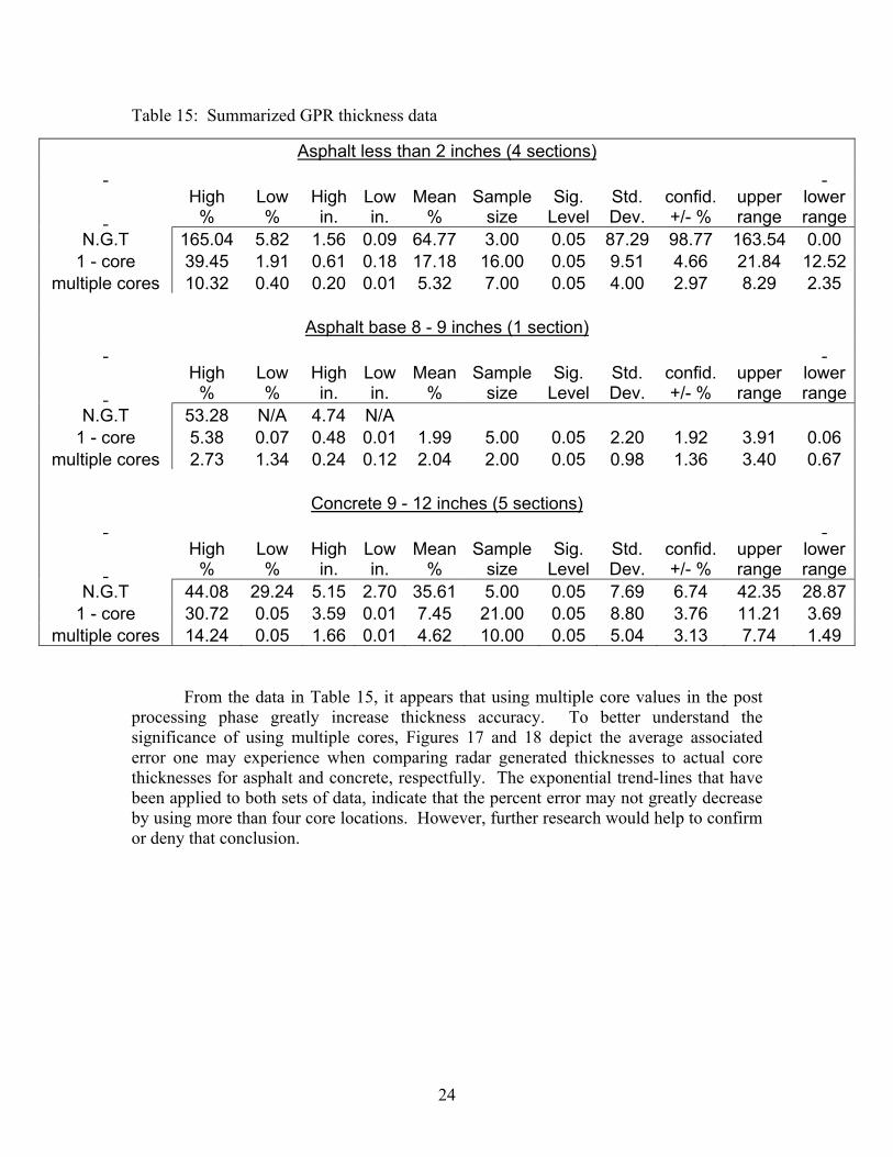
6.0 Summary of Data and Results The results from the previous report section have been summarized below in an effort to better understand the thickness accuracy produced by GSSI’s GPR Sir 10 B using a 1.0 GHz. air-launched horn antenna (Table 15). In addition, ninety-five percent confidence levels have also been assigned to the summarized data in Table 15. These values indicate the degree of accuracy one may expect ninety-five percent of the time when using zero, one, and multiple ground truth points when processing pavement layer thicknesses as outlined in Appendix A. Note, multiple ground truth points consist of data processed with two, three, and four cores.
24
Table 15: Summarized GPR thickness data
From the data in Table 15, it appears that using multiple core values in the post processing phase greatly increase thickness accuracy. To better understand the significance of using multiple cores, Figures 17 and 18 depict the average associated error one may experience when comparing radar generated thicknesses to actual core thicknesses for asphalt and concrete, respectfully. The exponential trend-lines that have been applied to both sets of data, indicate that the percent error may not greatly decrease by using more than four core locations. However, further research would help to confirm or deny that conclusion.
Asphalt less than 2 inches (4 sections)
High
% Low %
High in.
Low in.
Mean %
Sample size
Sig. Level
Std. Dev.
confid. +/- %
upper range
lower range
N.G.T 165.04 5.82 1.56 0.09 64.77 3.00 0.05 87.29 98.77 163.54 0.00 1 - core 39.45 1.91 0.61 0.18 17.18 16.00 0.05 9.51 4.66 21.84 12.52
multiple cores 10.32 0.40 0.20 0.01 5.32 7.00 0.05 4.00 2.97 8.29 2.35
Asphalt base 8 - 9 inches (1 section)
High
% Low %
High in.
Low in.
Mean %
Sample size
Sig. Level
Std. Dev.
confid. +/- %
upper range
lower range
N.G.T 53.28 N/A 4.74 N/A 1 - core 5.38 0.07 0.48 0.01 1.99 5.00 0.05 2.20 1.92 3.91 0.06
multiple cores 2.73 1.34 0.24 0.12 2.04 2.00 0.05 0.98 1.36 3.40 0.67
Concrete 9 - 12 inches (5 sections)
High
% Low %
High in.
Low in.
Mean %
Sample size
Sig. Level
Std. Dev.
confid. +/- %
upper range
lower range
N.G.T 44.08 29.24 5.15 2.70 35.61 5.00 0.05 7.69 6.74 42.35 28.871 - core 30.72 0.05 3.59 0.01 7.45 21.00 0.05 8.80 3.76 11.21 3.69
multiple cores 14.24 0.05 1.66 0.01 4.62 10.00 0.05 5.04 3.13 7.74 1.49

25
Asphalt - Ground Truth Summary Data
0
5
10
15
20
25
30
35
40
45
50
55
60
65
-1 0 1 2 3 4 5
number of cores
perc
enta
ge zero cores
one coretwo coresthree coresfour coresaverage
Figure 17: Asphalt—ground truth summary
Concrete - Ground Truth Summary
0
5
10
15
20
25
30
35
40
45
50
-1 0 1 2 3 4 5
number of cores
perc
enta
ge
zero coresone coretwo coresthree coresfour coresaverage
Figure 18: Concrete—ground truth summary

26
7.0 Pavement Layer Thickness Results from Other Research Institutions To date, there are several other academic research institutions that have used radar technology to determine pavement layer thicknesses. Although their data has not been obtained from the same brand of equipment as evaluated in this report, all tests have been conducted using a 1.0 GHz air launched horn antenna. A brief overview of their results has been included below. 7.1 Texas Transportation Institute
1. Recent studies of using Ground Penetrating Radar to determine pavement layer thickness yielded accuracies of +/- 5% to 7.5% or +/- 0.33 inches for asphalt thickness and +/- 9.5% or +/- 0.77 inches for base thickness.6
7.2 Infrasense Inc.
1. GPR was used to determine the pavement layer thickness for ten SHRP Long Term Pavement Performance (LTPP) asphalt sections ranging from 3 to 16 inches. The evaluation showed deviations from the cores of +/- 8% for blind evaluations and +/- 5% when calibration cores were used. 7
2. Four Texas SHRP asphalt pavement test sites resulted in radar prediction accuracies for asphalt thickness within +/- 0.32 inches or +/- 5% when using radar alone. When one calibration core was used per site, the accuracy was improved to +/- 0.11 inches. The accuracy of the radar predictions for base thickness was within +/- 1.00 inch. The nominal layer thickness at these sites ranged from 1 to 8 inches of asphalt and 6 to 10 inches of base. 7
7.3 Florida DOT State Project 99700-7550
1. Of five sites considered in the demonstration of radar’s capability to predict layer thicknesses, the means of the blind predictions for asphalt surface thickness on three sites were within 0.1 inch or 2 percent of the corresponding measured core. However, one site underestimated the asphalt thickness by over 1 inch. In regards to base thickness, blind radar results show a deviation from core values between 0 to 2.1 inches. The calculated means of the predicted base thicknesses were found, on average, to be within 0.9 inches of the measured core value in the blind comparisons. However, the differences between predicted and measured means for base thickness were reduced to within 0.5 inches after calibration. 2

27
8.0 Federal Communication Commission (FCC)
Recently, the Federal Communication Commission (FCC) set out regulations enforcing restrictions on using ground penetrating radar. The major concern is how ground penetrating radar is affecting/interfering with other radar/radio waves being transmitted in the same frequency range. The FCC wants to make sure that radio services, especially ones that deal with public safety, are protected, secured, and not interrupted by G.P.R. The National Telecommunications and Information Administration (NTIA) also want to ensure that precautions are taken to protect vital federal government operations from G.P.R. interference. Currently, the new restrictions allow the operation of ground penetrating radar by law enforcement, fire and rescue organizations, scientific research institutions, commercial mining companies, and construction companies. However, new G.P.R. equipment must be operated below 960 MHz or in the frequency band of 3.1 – 10.6 GHz, unless an organization has registered their equipment with the F.C.C. by October 15, 2002.8
9.0 Suggestions
After collecting, processing, and analyzing the collected radar data that has been discussed in this report, it is concluded that with some improvements radar technology can be used as a viable source for determining pavement layer thicknesses. These improvements consist of simplifying the post-processing phase for determining pavement layer thickness, accurately addressing a potential source of error in thin pavement layers known as double reflection, and further researching the appropriate number of actual cores needed to determine accurate pavement layer thicknesses.
As seen in appendix A, the techniques used to post-process the collected radar data in this report was comprised of a twenty-step process. Had any of these steps been deleted or altered it is highly likely different results would have been produced. The post-processing process needs to be simplified and/or automated. In addition, it would be beneficial if the post processing process was placed in a format that does not take a highly trained and/or skilled operator to determine the results.
Although some of the thickness results reported earlier in this report are within acceptable QA/QC ranges for pavement layers less than two inches. It is uncertain if the results could be improved by addressing what has been titled by the Texas Transportation Institute as “double reflection”. They define double reflection as an overlap in the surface and base reflection for pavement layers less than three inches.4 To eliminate this error, they have developed a surface removal technique that effectively removes the surface reflection from the trace and leaves the reflections from the lower pavement interfaces. A further explanation of this surface removal process may be viewed in Texas Transportation Institute’s report titled “Implementation of the Texas ground penetrating radar system”.
Some attempt has been made in this report to define the actual number of cores needed to improve layer thickness calculations. Although the preliminary results indicate that four cores are sufficient to obtain an acceptable degree of accuracy for asphalts, more research in this area would permit a more definitive result.

28
10.0 Conclusions The use of Ground Penetrating Radar (GPR) to determine pavement layer
thickness for both asphalts and concrete appears to be promising. As shown throughout this report many of the surface layer thicknesses determined by GPR, fell within the tolerance guidelines one would use for QA/QC in Kentucky. However, it is highly advised that calibration cores be used when post processing radar data to achieve the most accurate results.
When comparing surface layer thickness between GPR, calibrated with multiple core data, and actual measured cores one may expect GPR results to range between:
• Asphalt less than two inches:
o +/-10.32% to +/-0.40% o +/-0.20 to +/-0.01 inches
• Asphalt bases of eight to nine inches: o +/-2.73% to +/-1.34% o +/-0.24 to +/-0.12 inches
• Concrete nine to twelve inches: o +/-14.24 to +/-0.05% o +/-1.66 to +/-0.01 inches
Although additional test were conducted during this study to determine GPR’s
repeatability on dry pavements, GPR’s ability to determine pavement layer thicknesses in wet conditions, and to define how many actual field cores need to be taken to accurately post-process radar data into thickness values, it is felt that these areas may need to be further researched. Additionally it is felt that further development is needed in both the data collection and data post processing phases to help GPR be a more user friendly tool to determine pavement layer thicknesses.

29
APPENDIX A
Radan “Step-by-Step Post Processing Process”
1) Open View-Customize, Source File = folder with raw data, Output file = folder for processed data, change linear units
2) Open Calibration File 3) Click on FIR Filter button, under vertical filters set Low Pass = 3000,
High Pass = 250, filter type = Box Car, save file with the word “filter” at the end of the previously named calibration file
4) Check O-scope mode to make sure the position is correct 5) If position is not correct, go back to Linescan Mode and click on Position/Range
button and adjust. Save the filename with “adj” at the end. 6) Click on Generate Horn Calibration File. Change antenna type to 1GHz Horn
(4108). Make sure the generated horn calibration file has a short downward white line to it. If not, use the scissors to cut the upward motion off. Save it as the original calibration file name with “ghc” at the end.
7) Close all calibration files 8) Open Raw data file to process 9) Apply filters using the same settings as the calibration file 10) Click on Horn Reflection Picking, choose the correct calibration file, continue to
click next using default settings. Save with “hrp” at the end of the filename. 11) Click on Horn Layer Interpretation. Change layer continuity threshold to where it
is more than double the scans per unit (ex. If its one scan per 20 ft, make the layer continuity threshold 41) and the number of output layers to 1. Keep clicking Next using the default settings. Save the file with “hli” at the end of the original filename.
12) Click on Interactive Interpretation. Click on ASCII file button and choose the “.lay file” click OK.
13) Right click – other options, change layers to 1 under global tab. 14) Right click – pick options – single point, clean up random points 15) Right click – ground truth, enter core values and choose layer 1 and not targets 16) Under the pick options dialogue box choose select range and highlight points.
Right click – pick modified options – change pick velocity. 17) Under layer velocity calculation dialogue box, click core data. If you want a file
that has no ground truth, click automatic in this dialogue box instead of core data. 18) Additional ground truth points can be added as needed and the velocities will
automatically be corrected. Check the spreadsheet to make sure there are no zeros located under the depth column. If there is, right click on “z or depth” and select “>0”. This will delete all the points with a depth of zero.
19) Right click – save changes – new filename, same it as the original filename with “gt” at the end.
20) To process the data in excel open the original filename with “gt.lay” at the end.

30
References 1. Saarenketo, Timo, and Scullion, Tom (1994), “Ground Penetrating Radar
Applications on Roads and Highways,” Texas Transportation Institute, Research Report 1923-2F, Texas Transportation Institute, College Station, Texas, Nov. 1994.
2. Fernando, Emmanuel G., and Maser, Kenneth R., “Development of a Procedure
for the Automated Collection of Flexible Pavement Layer Thicknesses and Materials: Phase I: Demonstration of Existing Ground Penetrating Radar Technology,” Florida DOT State Project 99700-7550, Texas Transportation Institute, College Station, Texas 77843.
3. Scullion, Tom, and Lau, Chun-Lok, and Chen, Yiqing (1994), “Implementation of
the Texas Ground Penetrating Radar System,” Texas Transportation Institute, Research Report 1233-1, Texas Transportation Institute, College Station, Texas, Apr. 1994
4. Scullion, Tom, and Chen, Yiqing (1999), “Using Ground-Penetrating Radar for
Real-Time Quality Control Measurements on New HMA Surfaces,” Texas Transportation Institute, Research Report 1702-5, Texas Transportation Institute, College Station, Texas, Nov. 1999.
5. “Standard Specifications for Road and Bridge Construction,” Kentucky 2000
Transportation Cabinet/Department of Highways, pg 403-5, 501-17. 6. Maser, Ken, and Scullion, Tom (1992), “Influence of Asphalt Layering and
Surface Treatments on Asphalt and Base Layer Thickness Computations Using Radar,” Texas Transportation Institute, Research Report 1923-1, Texas Transportation Institute, College Station, Texas, Sept. 1992.
7. Maser, Kenneth (1994), “Ground Penetrating Radar Surveys to Characterize
Pavement Layer Thickness Variations at GPS Sites,” INFRASENSE Inc., Research Report SHRP-P-397, Strategic Highway Research Program, National Research Council, Washington, DC, Apr. 1994.
8. Federal Communications Commission, “New public safety applications and
broadband internet access among uses envisioned by FCC authorization of ultra-wideband technology”, February 14, 2002. News.


