Introduction Geothermal heat production from sedimentary basins in non magmatic settings can provide an important source of renewable energy in the future (e.g. IEA, 2011). In these settings hot water is produced from aquifers (water bearing layers) at large depth (>1 km; Ungemach et al., 2005). The energy is extracted through a heat exchanger and used for spatial heating, adsorption cooling or greenhouse heating. After cooling the water is reinjected. The well configuration consisting of an injection and production well is generally referred to as a doublet. The produced thermal power (E) is linearly proportional to the temperature difference of produced and reinjected temperature (ΔT = T production –T injection ) and flow rate of the produced water (Q (m 3 /h); Van Wees et al., this issue): E [MWth] ≈ 1200 ΔT · Q (Eq. 1) For a particular aquifer the production temperature T production can be predicted from the geothermal gradient and the depth of the aquifer. The temperature of the produced water at geo- thermal production flow rates is almost equal to the temperature of the aquifer rocks. The subsurface of the Netherlands shows 621 Netherlands Journal of Geosciences — Geologie en Mijnbouw | 91 – 4 | 2012 Netherlands Journal of Geosciences — Geologie en Mijnbouw | 91 – 4 | 621 - 636 | 2012 Reservoir characterisation of aquifers for direct heat production: Methodology and screening of the potential reservoirs for the Netherlands M.P.D. Pluymaekers 1,* , L. Kramers 1 , J.-D. van Wees 1,2 , A. Kronimus 1 , S. Nelskamp 1 , T. Boxem 1 & D. Bonté 1 1 TNO – Geological Survey of the Netherlands, P.O. Box 80015, 3508 TA Utrecht, the Netherlands. 2 Utrecht University, Faculty of Geosciences, P.O. Box 80021, 3508 TA Utrecht, the Netherlands. * Corresponding author. Email: [email protected]. Manuscript received: October 2011, accepted: August 2012 Abstract Geothermal low enthalpy heat in non-magmatic areas can be produced by pumping hot water from aquifers at large depth (>1 km). Key parameters for aquifer performance are temperature, depth, thickness and permeability. Geothermal exploration in the Netherlands can benefit considerably from the wealth of oil and gas data; in many cases hydrocarbon reservoirs form the lateral equivalent of geothermal aquifers. In the past decades subsurface oil and gas data have been used to develop 3D models of the subsurface structure. These models have been used as a starting point for the mapping of geothermal reservoir geometries and its properties. A workflow was developed to map aquifer properties on a regional scale. Transmissivity maps and underlying uncertainty have been obtained for 20 geothermal aquifers. Of particular importance is to take into account corrections for maximum burial depth and the assessment of uncertainties. The mapping of transmissivity and temperature shows favorable aquifer conditions in the northern part of the Netherlands (Rotliegend aquifers), while in the western and southern parts of the Netherlands aquifers of the Triassic and Upper Cretaceous / Jurassic have high prospectivity. Despite the high transmissivity of the Cenozoic aquifers, the limited depth and temperature reduce the prospective geothermal area significantly. The results show a considerable remaining uncertainty of transmissivity values, due to lack of data and heterogeneous spatial data distribution. In part these uncertainties may be significantly reduced by adding well test results and facies parameters for the map interpolation in future work. For underexplored areas this bears a significant risk, but it can also result in much higher flowrates than originally expected, representing an upside in project performance. Keywords: Geothermal energy, regional transmissivity mapping, aquifer.
Transcript
Introduction
Geothermal heat production from sedimentary basins in nonmagmatic settings can provide an important source of renewableenergy in the future (e.g. IEA, 2011). In these settings hotwater is produced from aquifers (water bearing layers) at largedepth (>1 km; Ungemach et al., 2005). The energy is extractedthrough a heat exchanger and used for spatial heating, adsorptioncooling or greenhouse heating. After cooling the water isreinjected. The well configuration consisting of an injectionand production well is generally referred to as a doublet.
The produced thermal power (E) is linearly proportional to the temperature difference of produced and reinjectedtempera ture (ΔT = Tproduction – Tinjection) and flow rate of theproduced water (Q (m3/h); Van Wees et al., this issue):
E [MWth] ≈ 1200 ΔT · Q (Eq. 1)
For a particular aquifer the production temperature Tproduction
can be predicted from the geothermal gradient and the depthof the aquifer. The temperature of the produced water at geo -thermal production flow rates is almost equal to the tempera tureof the aquifer rocks. The subsurface of the Netherlands shows
621Netherlands Journal of Geosciences — Geologie en Mijnbouw | 91 – 4 | 2012
Netherlands Journal of Geosciences — Geologie en Mijnbouw | 91 – 4 | 621 - 636 | 2012
Reservoir characterisation of aquifers for direct heat production: Methodology and screening of the potential reservoirs for the Netherlands
M.P.D. Pluymaekers1,*, L. Kramers1, J.-D. van Wees1,2, A. Kronimus1, S. Nelskamp1, T. Boxem1 & D. Bonté1
1 TNO – Geological Survey of the Netherlands, P.O. Box 80015, 3508 TA Utrecht, the Netherlands.
2 Utrecht University, Faculty of Geosciences, P.O. Box 80021, 3508 TA Utrecht, the Netherlands.
an average geothermal gradient of approximately 31 °C/km,although the temperature gradient can vary between 25 and 40 °C/km depending on geological setting (Bonté et al., thisissue). Given an average surface temperature of 10 °C, thismeans that at 1200 m depth temperatures are sufficiently highfor greenhouse heating (Tproduction > 45 °C) and at 1800 mdepth temperatures are sufficiently high for spatial heating(Tproduction > 65 °C). In any case, aquifers shallower than 1000m depth are not favorable for heat production. The flow rate Qdepends on the hydrological properties of the aquifer andengineering design of the wells (Van Wees et al., this issue).The transmissivity (the mathematical product of aquifer thick -ness and permeability) significantly determines the flow ratewhich can be achieved as the result of a pressure difference
applied to the wells. In summary, temperature, depth, thick -ness and porosity/permeability of aquifers are key parametersto obtain for a proper geothermal characterisation.
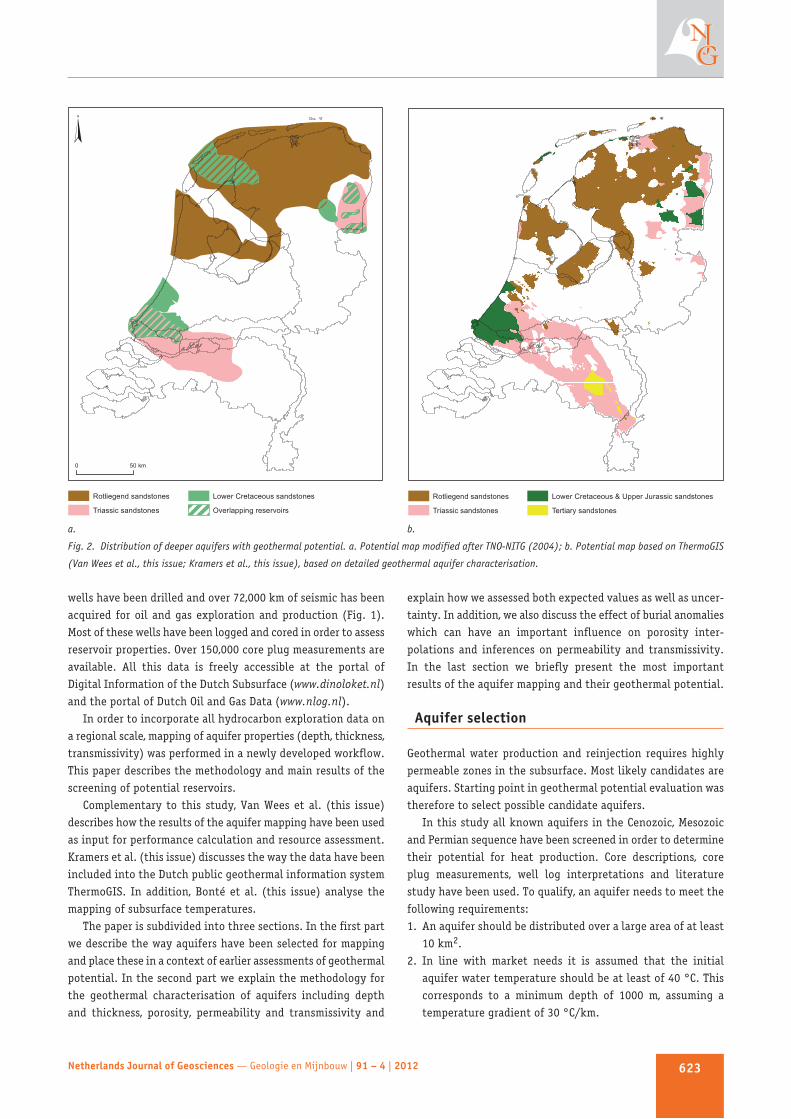
Earlier studies on the geothermal potential of the Netherlands(TNO-NITG, 2004; Van Doorn & Rijkers, 2002) were based on arather qualitative assessment, not taking into account detailedmapping and well property information. These studies identifiedaquifers in three major stratigraphic group including thePermian Rotliegendes, Triassic and Early Cretaceous (Fig. 2a).
In the Netherlands, prospective areas for geothermal explo -ra tion largely correspond to areas in which hydrocarbonexplora tion and production has taken or takes place. Therefore,geothermal exploration can take considerable advantage fromthe existing oil and gas data. Over the past 30 years over 5000
Netherlands Journal of Geosciences — Geologie en Mijnbouw | 91 – 4 | 2012622
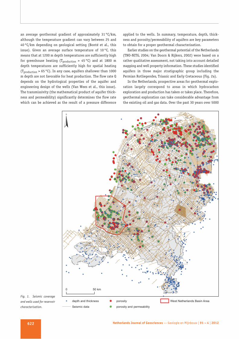
Fig. 1. Seismic coverage
and wells used for reservoir
characterisation.
wells have been drilled and over 72,000 km of seismic has beenacquired for oil and gas exploration and production (Fig. 1).Most of these wells have been logged and cored in order to assessreservoir properties. Over 150,000 core plug measure ments areavailable. All this data is freely accessible at the portal ofDigital Information of the Dutch Subsurface (www.dinoloket.nl)and the portal of Dutch Oil and Gas Data (www.nlog.nl).
In order to incorporate all hydrocarbon exploration data ona regional scale, mapping of aquifer properties (depth, thickness,transmissivity) was performed in a newly developed workflow.This paper describes the methodology and main results of thescreening of potential reservoirs.
Complementary to this study, Van Wees et al. (this issue)describes how the results of the aquifer mapping have been usedas input for performance calculation and resource assessment.Kramers et al. (this issue) discusses the way the data have beenincluded into the Dutch public geothermal information systemThermoGIS. In addition, Bonté et al. (this issue) analyse themapping of subsurface temperatures.
The paper is subdivided into three sections. In the first partwe describe the way aquifers have been selected for mappingand place these in a context of earlier assessments of geothermalpotential. In the second part we explain the methodology forthe geothermal characterisation of aquifers including depthand thickness, porosity, permeability and transmissivity and
explain how we assessed both expected values as well as uncer -tainty. In addition, we also discuss the effect of burial anomalieswhich can have an important influence on porosity inter -polations and inferences on permeability and transmissivity.In the last section we briefly present the most importantresults of the aquifer mapping and their geothermal potential.
Aquifer selection
Geothermal water production and reinjection requires highlypermeable zones in the subsurface. Most likely candidates areaquifers. Starting point in geothermal potential evaluation wastherefore to select possible candidate aquifers.
In this study all known aquifers in the Cenozoic, Mesozoicand Permian sequence have been screened in order to determinetheir potential for heat production. Core descriptions, coreplug measurements, well log interpretations and literaturestudy have been used. To qualify, an aquifer needs to meet thefollowing requirements: 1. An aquifer should be distributed over a large area of at least
10 km2.2. In line with market needs it is assumed that the initial
aquifer water temperature should be at least of 40 °C. Thiscorresponds to a minimum depth of 1000 m, assuming atempera ture gradient of 30 °C/km.
Netherlands Journal of Geosciences — Geologie en Mijnbouw | 91 – 4 | 2012 623
a.
Fig. 2. Distribution of deeper aquifers with geothermal potential. a. Potential map modified after TNO-NITG (2004); b. Potential map based on ThermoGIS
(Van Wees et al., this issue; Kramers et al., this issue), based on detailed geothermal aquifer characterisation.
b.
3. An aquifer should have a minimum thickness of 20 m over asignificant portion of the distribution area. Aquifers thinnerthan 20 m are not expected to meet a minimum transmis sivityof 10 Dm, as defined as a cut-off by Kramers et al. (this issue).
This approach resulted in a selection of 20 aquifers (Table 1).Compared to the potential aquifer map presented in Lokhorst &Wong (2007; Fig. 2a), Cenozoic aquifers are now incorporated.The workflow process of mapping geothermal transmissivity forthese 20 aquifers has resulted in a significantly more detailedextend of potential aquifers, outlined in Fig. 2b.
Reservoir characterisation
In this paper we describe a regional reservoir characterisationworkflow which takes existing 3D subsurface models, core plugdata and log data from wells as input. The 3D models of thesubsurface provided the boundaries of the main stratigraphicgroups (e.g. base Jurassic; TNO-NITG, 2004; Duin et al., 2006).
The number of published studies on flow properties of reservoirsis rather limited, because it was mainly done in-house by oilcompanies. Wells and associated exploration studies have notbeen uniformly distributed throughout the area but focussed onstructurally high areas and in areas with proven hydrocarbonplays. So, despite hydrocarbon and geothermal exploration targetsimilar stratigraphic levels, the spatial data density is hetero -geneous.
The process of mapping (maximum burial) depth and thicknessof aquifers is presented first. Subsequently, the mapping oftransmissivity, which is subdivided into five process steps, isdescribed in the sections below. The workflow predicts averagevalues as well as underlying uncertainty.
The workflow steps (Fig. 3) rely on a number of key assump -tions:a. An average value for permeability is assumed for individual
aquifers. The mapped thickness of the aquifer is not furtherdifferentiated to net pay zones through a cut-off value inpermeability. Although it can be argued that average values
Netherlands Journal of Geosciences — Geologie en Mijnbouw | 91 – 4 | 2012624
Table 1. List of aquifers included in ThermoGIS.
Stratigraphic unit Stratigraphic Group ThermoGIS Stratigraphic Stratigraphic Member ThermoGIS
(Upper) Slochteren and Lower Slochteren RO-Stacked
of permeability would be higher when net pay zones aretaken into account, the transmissivity of the aquifer will notchange as the thickness is proportionally reduced. A draw -back of averaging permeability is the masking of possiblepreferential flow through high perm zones. This will increaseuncertainty in doublet lifetime regarding to breakthroughof cold injection water.
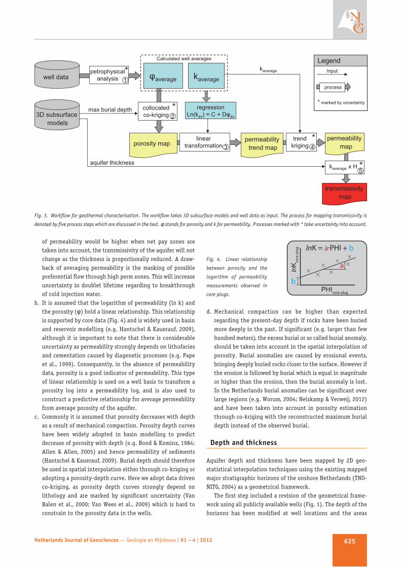
b. It is assumed that the logarithm of permeability (ln k) andthe porosity (φ) hold a linear relationship. This relationshipis supported by core data (Fig. 4) and is widely used in basinand reservoir modelling (e.g. Hantschel & Kauerauf, 2009),although it is important to note that there is considerableuncertainty as permeability strongly depends on lithofaciesand cementation caused by diagenetic processes (e.g. Papeet al., 1999). Consequently, in the absence of permeabilitydata, porosity is a good indicator of permeability. This typeof linear relationship is used on a well basis to transform aporosity log into a permeability log, and is also used toconstruct a predictive relationship for average permeabilityfrom average porosity of the aquifer.
c. Commonly it is assumed that porosity decreases with depthas a result of mechanical compaction. Porosity depth curveshave been widely adopted in basin modelling to predictdecrease of porosity with depth (e.g. Bond & Kominz, 1984;Allen & Allen, 2005) and hence permeability of sediments(Hantschel & Kauerauf, 2009). Burial depth should thereforebe used in spatial interpolation either through co-kriging oradopting a porosity-depth curve. Here we adopt data drivenco-kriging, as porosity depth curves strongly depend onlithology and are marked by significant uncertainty (VanBalen et al., 2000; Van Wees et al., 2009) which is hard toconstrain to the porosity data in the wells.
d. Mechanical compaction can be higher than expectedregarding the present-day depth if rocks have been buriedmore deeply in the past. If significant (e.g. larger than fewhundred meters), the excess burial or so called burial anomaly,should be taken into account in the spatial interpolation ofporosity. Burial anomalies are caused by erosional events,bringing deeply buried rocks closer to the surface. However ifthe erosion is followed by burial which is equal in magnitudeor higher than the erosion, then the burial anomaly is lost.In the Netherlands burial anomalies can be significant overlarge regions (e.g. Worum, 2004; Nelskamp & Verweij, 2012)and have been taken into account in porosity estimationthrough co-kriging with the reconstructed maximum burialdepth instead of the observed burial.
Depth and thickness
Aquifer depth and thickness have been mapped by 2D geo -statistical interpolation techniques using the existing mappedmajor stratigraphic horizons of the onshore Netherlands (TNO-NITG, 2004) as a geometrical framework.
The first step included a revision of the geometrical frame -work using all publicly available wells (Fig. 1). The depth of thehorizons has been modified at well locations and the areas
Netherlands Journal of Geosciences — Geologie en Mijnbouw | 91 – 4 | 2012 625
Input
process
Legend
* marked by uncertainty
average
transmissivity map
well data
3D subsurface models
porosity map
petrophysical analysis kaverage
collocated co-kriging
permeability trend map
permeability map
max burial depth
linear transformation
regression Ln(kav) = C + D av
kaverage x H
aquifer thickness
Calculated well averages
kaverage
trend kriging
*
*
*
* 1
2
3 4
5
Fig. 3. Workflow for geo thermal characterisation. The workflow takes 3D subsurface models and well data as input. The process for mapping trans missivity is
denoted by five process steps which are discussed in the text. φ stands for porosity and k for permeability. Processes marked with * take uncertainty into account.
lnK
core
plu
g
PHIcore plug
b
a
lnK = a·PHI + bFig. 4. Linear relationship
between porosity and the
logarithm of permeability
measurements observed in
core plugs.
surrounding the well location using a kriged correction gridbased on the misfit between well information and horizons.Kriging is an interpolation method where the interpolated valueis a distance-weighted average of the known datapoints. Thespatial correlation and accompanying variance of the datapoints is characterised in a variogram. The variance (uncertainty)of the interpolated value will increase as the distance toknown datapoints increases.
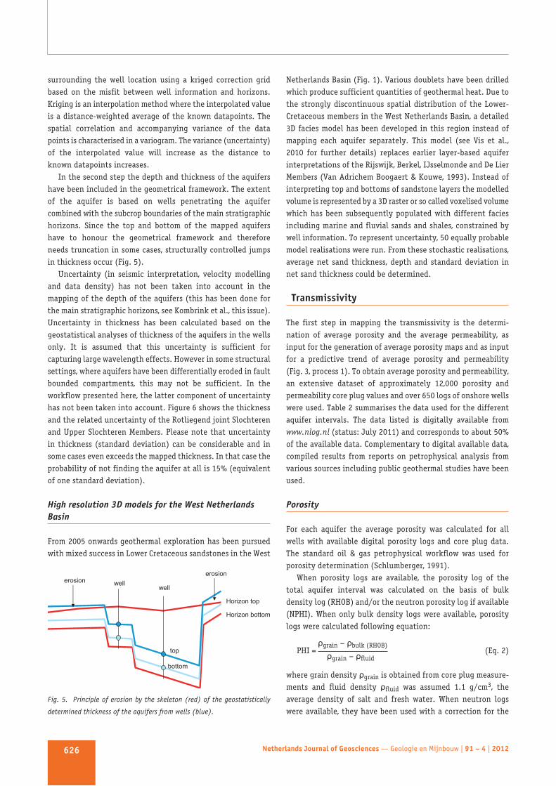
In the second step the depth and thickness of the aquifershave been included in the geometrical framework. The extentof the aquifer is based on wells penetrating the aquifercombined with the subcrop boundaries of the main stratigraphichorizons. Since the top and bottom of the mapped aquifershave to honour the geometrical framework and thereforeneeds truncation in some cases, structurally controlled jumpsin thickness occur (Fig. 5).
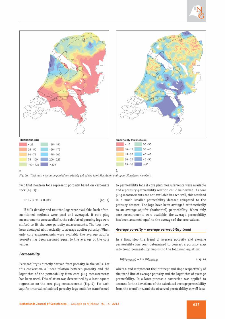
Uncertainty (in seismic interpretation, velocity modellingand data density) has not been taken into account in themapping of the depth of the aquifers (this has been done forthe main stratigraphic horizons, see Kombrink et al., this issue).Uncertainty in thickness has been calculated based on thegeostatistical analyses of thickness of the aquifers in the wellsonly. It is assumed that this uncertainty is sufficient forcapturing large wavelength effects. However in some structuralsettings, where aquifers have been differentially eroded in faultbounded compartments, this may not be sufficient. In theworkflow presented here, the latter component of uncertaintyhas not been taken into account. Figure 6 shows the thicknessand the related uncertainty of the Rotliegend joint Slochterenand Upper Slochteren Members. Please note that uncertaintyin thickness (standard deviation) can be considerable and insome cases even exceeds the mapped thickness. In that case theprobability of not finding the aquifer at all is 15% (equivalentof one standard deviation).
High resolution 3D models for the West NetherlandsBasin
From 2005 onwards geothermal exploration has been pursuedwith mixed success in Lower Cretaceous sandstones in the West
Netherlands Basin (Fig. 1). Various doublets have been drilledwhich produce sufficient quantities of geothermal heat. Due tothe strongly discontinuous spatial distribution of the Lower-Cretaceous members in the West Netherlands Basin, a detailed3D facies model has been developed in this region instead ofmapping each aquifer separately. This model (see Vis et al.,2010 for further details) replaces earlier layer-based aquiferinterpretations of the Rijswijk, Berkel, IJsselmonde and De LierMembers (Van Adrichem Boogaert & Kouwe, 1993). Instead ofinterpreting top and bottoms of sandstone layers the modelledvolume is represented by a 3D raster or so called voxelised volumewhich has been subsequently populated with different faciesincluding marine and fluvial sands and shales, constrained bywell information. To represent uncertainty, 50 equally probablemodel realisations were run. From these stochastic realisations,average net sand thickness, depth and standard deviation innet sand thickness could be determined.
Transmissivity
The first step in mapping the transmissivity is the determi -nation of average porosity and the average permeability, asinput for the generation of average porosity maps and as inputfor a predictive trend of average porosity and permeability(Fig. 3, process 1). To obtain average porosity and permeability,an extensive dataset of approximately 12,000 porosity andpermeability core plug values and over 650 logs of onshore wellswere used. Table 2 summarises the data used for the differentaquifer intervals. The data listed is digitally available fromwww.nlog.nl (status: July 2011) and corresponds to about 50%of the available data. Complementary to digital available data,compiled results from reports on petrophysical analysis fromvarious sources including public geothermal studies have beenused.
Porosity
For each aquifer the average porosity was calculated for allwells with available digital porosity logs and core plug data.The standard oil & gas petrophysical workflow was used forporosity determination (Schlumberger, 1991).
When porosity logs are available, the porosity log of thetotal aquifer interval was calculated on the basis of bulkdensity log (RHOB) and/or the neutron porosity log if available(NPHI). When only bulk density logs were available, porositylogs were calculated following equation:
ρgrain – ρbulk (RHOB)PHI = ρgrain – ρfluid
(Eq. 2)
where grain density ρgrain is obtained from core plug measure -ments and fluid density ρfluid was assumed 1.1 g/cm3, theaverage density of salt and fresh water. When neutron logswere available, they have been used with a correction for the
Netherlands Journal of Geosciences — Geologie en Mijnbouw | 91 – 4 | 2012626
top
bottom
well well
Horizon top
Horizon bottom
erosion erosion
Fig. 5. Principle of erosion by the skeleton (red) of the geostatistically
determined thickness of the aquifers from wells (blue).
fact that neutron logs represent porosity based on carbonaterock (Eq. 3):
PHI = NPHI + 0.045 (Eq. 3)
If bulk density and neutron logs were available, both afore -mentioned methods were used and averaged. If core plugmeasurements were available, the calculated porosity logs wereshifted to fit the core-porosity measurements. The logs havebeen averaged arithmetically to average aquifer porosity. Whenonly core measurements were available the average aquiferporosity has been assumed equal to the average of the corevalues.
Permeability
Permeability is directly derived from porosity in the wells. Forthis conversion, a linear relation between porosity and thelogarithm of the permeability from core plug measurementshas been used. This relation was determined by a least-squareregression on the core plug measurements (Fig. 4). For eachaquifer interval, calculated porosity logs could be transformed
to permeability logs if core plug measurements were availableand a porosity-permeability relation could be derived. As coreplug measurements are not available in each well, this resultedin a much smaller permeability dataset compared to theporosity dataset. The logs have been averaged arithmeticallyto an average aquifer (horizontal) permeability. When onlycore measurements were available, the average permeabilityhas been assumed equal to the average of the core values.
Average porosity – average permeability trend
In a final step the trend of average porosity and averagepermeability has been determined to convert a porosity mapinto trend permeability map using the following equation:
ln(kaverage) = C + Dϕaverage (Eq. 4)
where C and D represent the intercept and slope respectively ofthe trend line of average porosity and the logarithm of averagepermeability. In a later process a correction was applied toaccount for the deviations of the calculated average permeabilityfrom the trend line, and the observed permeability at well loca -
Netherlands Journal of Geosciences — Geologie en Mijnbouw | 91 – 4 | 2012 627
Thickness (m)
< 25
25 - 50
50 - 75
75 - 100
100 - 125
125 - 150
150 - 175
175 - 200
200 - 225
> 225
Uncertainty thickness (m)
< 10
10 - 15
15 - 20
20 - 25
25 - 30
30 - 35
35 - 40
40 - 45
45 - 50
> 50
a.
Fig. 6a. Thickness with accompanied uncertainty (b) of the joint Slochteren and Upper Slochteren members.
b.
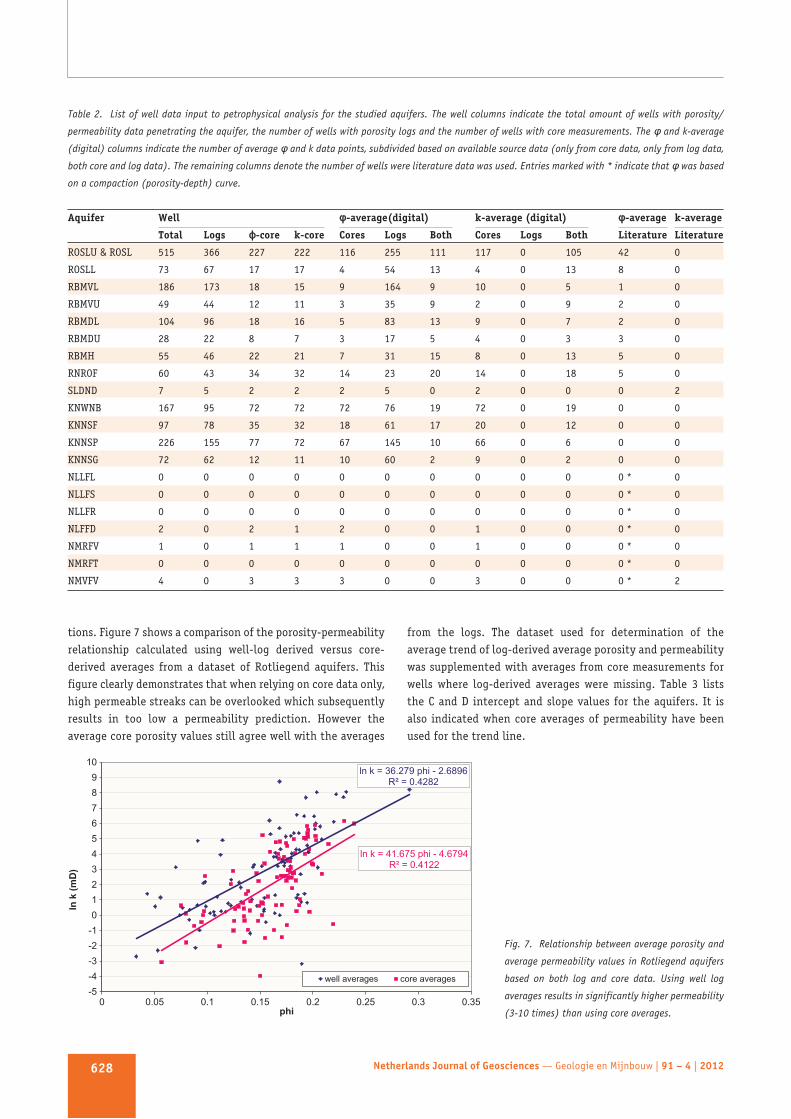
tions. Figure 7 shows a comparison of the porosity-permeabilityrelationship calculated using well-log derived versus core-derived averages from a dataset of Rotliegend aquifers. Thisfigure clearly demonstrates that when relying on core data only,high permeable streaks can be overlooked which subsequentlyresults in too low a permeability prediction. However theaverage core porosity values still agree well with the averages
from the logs. The dataset used for determination of theaverage trend of log-derived average porosity and permeabilitywas supplemented with averages from core measurements forwells where log-derived averages were missing. Table 3 liststhe C and D intercept and slope values for the aquifers. It isalso indicated when core averages of permeability have beenused for the trend line.
Netherlands Journal of Geosciences — Geologie en Mijnbouw | 91 – 4 | 2012628
Table 2. List of well data input to petrophysical analysis for the studied aquifers. The well columns indicate the total amount of wells with porosity/
permeability data penetrating the aquifer, the number of wells with porosity logs and the number of wells with core measurements. The φ and k-average
(digital) columns indicate the number of average φ and k data points, subdivided based on available source data (only from core data, only from log data,
both core and log data). The remaining columns denote the number of wells were literature data was used. Entries marked with * indicate that φ was based
on a compaction (porosity-depth) curve.
Aquifer Well φ-average(digital) k-average (digital) φ-average k-average
Total Logs ϕ-core k-core Cores Logs Both Cores Logs Both Literature Literature
average permeability values in Rotliegend aquifers
based on both log and core data. Using well log
averages results in significantly higher permeability
(3-10 times) than using core averages.
Burial anomaly reconstruction and porosity maps
As mentioned before, the mapview interpolation of the averageporosity was done with the collocated co-kriging method, inwhich the maximum burial depth as a second, collocated variablewas taken into account (Fig. 3, process 2). Collocated co-kriging interpolation (Xu et al., 1992) takes into account thecorrelation between primary data (porosity from well data) andsecondary data (burial depth from well and horizon data) whichis available throughout the entire model area. This means thatinterpolation of a porosity value away from the well locationwill also depend on burial depth.
In order to construct maximum burial, the excess burial orso called burial anomaly is added to the present-day burial. Inthe Netherlands various studies addressed burial anomaliesand have shown that they can be significant over large regions(e.g. Worum, 2004; Van Dalfsen et al., 2005; Van Wees et al.,2009; Luijendijk et al., 2011; Nelskamp & Verweij, 2012). Burialanomalies can be detected in various ways. In this paper weadopted a complementary approach to assess burial anomalies.For the structural inverted basins (De Jager, 2007), first orderburial anomaly values have been determined from structural
reconstruction as described in Van Wees et al. (2011). For theWest Netherlands Basin and Roer Valley Basin areas morereliable erosion estimates are derived from a detailed basinmodel for maturity modelling, calibrated to maturity parameters(Nelskamp & Verweij, 2012).
Major erosional phases occurred immediately after depositionof the Chalk Group (Laramide erosional phase) and the Schielandand Niedersachsen group (Late Kimmerian erosional phase). Toobtain the burial anomaly, the calculated erosion maps of theLaramide and the Late Kimmerian erosional phases have beensubtracted with the present day depth of respectively the baseNorth Sea Supergroup and base Rijnland Group. Thesecomplementary models (Fig. 8) show that both types of erosionestimates largely agree with discrepancies up to 30%. Sonicvelocities indicate larger deviations (Van Dalfsen et al., 2005),and suggest much higher erosion and burial anomalies in manyplaces. It is argued that these anomalies in sonic velocity maybe artefacts related to differences in lithology.
Taking into account burial anomalies results in a bettercorrelation in the porosity-depth relation (Figs 9, 10 and 11). Thisis particularly apparent for non-inverted basin margins whereporosity well data control is sparse. Here, an increase in porosityof up to 3% and a related increase in permeability up to a factor
Netherlands Journal of Geosciences — Geologie en Mijnbouw | 91 – 4 | 2012 629
Table 3. Intercept (C) and slope (D) of average porosity and average
natural logarithm of permeability (mD) of the different aquifers. The table
lists the amount of wells with logs and/or cores used for the trend and the
number of wells with only core data. Entries marked with * denote that
literature values were used. For the KNWNB aquifer, different modelling
approach was chosen (see Vis et al., 2010).
Aquifer Regression Data points
C D Logs Cores only
ROSLU & ROSL –1.88 0.319 105 116
ROSLL –2.27 0.288 13 4
RBMVL –4.11 0.498 5 9
RBMVU –2.82 0.454 9 2
RBMDL –3.62 0.437 7 5
RBMDU –1.38 0.330 3 3
RBMH –4.06 0.539 13 7
RNROF –0.41 0.298 18 14
SLDND 0.38 0.202 0 2
KNWNB - - - -
KNNSF –2.16 0.198 12 18
KNNSP –2.25 0.299 6 66
KNNSG 0.06 0.089 2 9
NLLFL * –1.49 0.242 0 0
NLLFS * –1.49 0.242 0 0
NLLFR * –1.49 0.242 0 0
NLFFD * –1.49 0.242 0 1
NMRFV * –1.49 0.242 0 1
NMRFT * –1.49 0.242 0 0
NMVFV * –1.49 0.242 0 3
0 50 km
Total Burial Anomalies (m)
50 - 250
250 - 500
500 - 750
750 - 1000
1000 - 1250
1250 - 1500
Basin modeling study area
Fig. 8. Total burial anomalies in meters from the geometric reconstruction,
partly complemented by results from basin modelling in the West
Netherlands Basin and the Roer Valley Graben (indicated by red polygon).
Netherlands Journal of Geosciences — Geologie en Mijnbouw | 91 – 4 | 2012630
R² = 0.3773
1000
1500
2000
2500
3000
3500
4000
0 0.05 0.1 0.15 0.2 0.25 0.3
dep
th (
m)
porosity
maximum burrial depth
R² = 0.2339
1000
1500
2000
2500
3000
3500
4000
0 0.05 0.1 0.15 0.2 0.25 0.3
dep
th (
m)
porosity
present depth
a.
Fig. 9a. Porosity-depth relationship after the correction for burial anomaly and (b) prior to correction.
b.
a.
Fig. 10 a. Porosity map taking maximum burial into account. b. Differential map of porosity of the Rotliegend geothermal aquifer adopting maximum
burial vs. adopting present day burial in the collocated co-kriging estimation. Red shaded areas are marked by increase, blue areas by decrease.
b.
of two were obtained. As a result, the prospectivity of basinflanks (with few data) of inverted basins (with most well datacontrol) can be significantly enhanced by incorporating burialanomalies.
Permeability and transmissivity
Average permeability maps are constructed in two steps. Firstthe average porosity map is converted to a permeability trendmap using equation 4 (Fig. 3, process 3). Subsequently, thepermeability map is obtained from trend kriging the (limitednumber of) kaverage data points whereby the permeabilitytrend map is used as trend input (Fig. 3, process 4). Trendkriging interpolates the residual values of the well data, andthe predictive values of the trend input map. The resultingpermeability map honours the data points and follows thepermeability trend when no hard permeability data is available.The transmissivity was calculated by multiplying the aquiferthickness with the obtained permeability (Fig. 3, process 5).
Workflow North Sea Group aquifers
The limited amount of data of North Sea Group aquifers did notallow the geostatistical approach as described above. Acompaction based porosity estimation is proposed instead(Athy, 1930), where porosity is a function of depth:
φ = φ-e(–kz) (Eq. 5)
where φ0 is 40% and k is 0.00031 (m–1; Hantschel & Kauerauf,2009). Figure 12 shows the porosity estimation and the dataavailable. The compaction curve overestimates the porosity atdepth below 1 km. Permeability was estimated based on a fixedporosity-permeability relation (Eq. 4, Table 3). Parameters ofthis relation were derived from a previous characterisation study
Netherlands Journal of Geosciences — Geologie en Mijnbouw | 91 – 4 | 2012 631
a.
Fig. 11 a. Permeability of the Rotliegend aquifer including the effect of burial anomalies; and b. the ratio of corrected and uncorrected permeability.
b.
10
15
20
25
30
35
40
45
0 1 2 3
poro
sity
(%
)
depth (km)
Compaction curve
All datapoints
Model datapoints
Fig. 12. Porosity estimation based on compaction (solid line) compared to
data used in the modelling workflow (purple). Green data represent all
available porosity data (on and offshore) of North Sea Group aquifers that
were not included in the aquifer selection.
of the Roer Valley Graben (Wiers, 2001). The resulting trans -missivity for the North Sea Group is a first estimate and shouldbe used with care, given the limited data available.
Uncertainty
The mapping workflow for deriving transmissivity did not incor -porate the effect of uncertainties. For uncertainty assessment,the following assumptions have been made:a. Porosity is normally distributed. b. The uncertainty of the calculated average porosity at the
wells is dependent on the data source. Uncertainty of logderived porosity is approximately 5%. This figure reflectsthe uncertainty related to fluid and grain density and com -position. Average porosity based only on core measurementscomprises a very limited part of the reservoir rock whichcauses the uncertainty to be higher. Comparison betweencore and log averages of the Rotliegend dataset (Fig. 7) showan uncertainty of approximately 10% for porosity derivedfrom core measurements only. Average values extracted fromliterature were based on full petrophysical analysis andtherefore uncertainty was assumed 3%.
c. Permeability is log-normally distributed.
The uncertainty of the interpolation of the porosity data-points is expressed as the standard deviation as a result fromkriging interpolation. The variogram is leading; the uncertaintyat the well position is incorporated in the variogram. Thestandard deviation of the permeability is given by the standarddeviation of the permeability trend (expressed as function ofφSD and slope D (Eq. 4)) and the standard deviation (SD) of thepermeability kriging (kaverage) SD as expressed in equation 6:
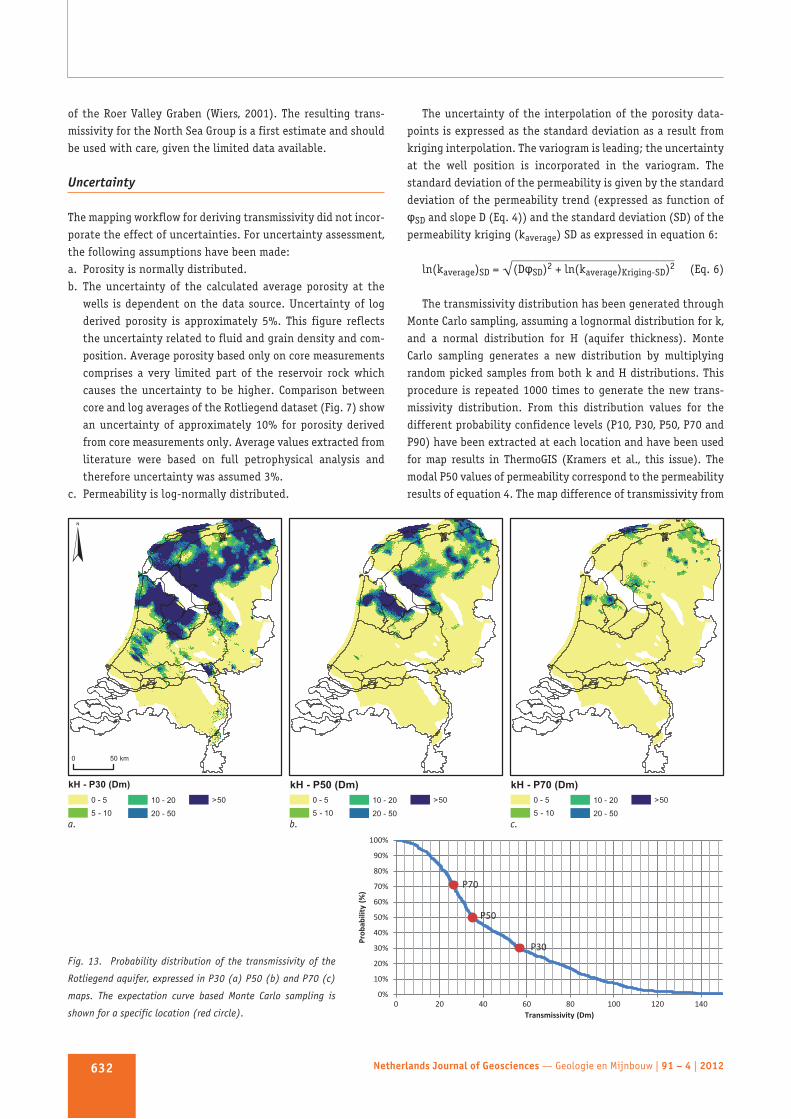
The transmissivity distribution has been generated throughMonte Carlo sampling, assuming a lognormal distribution for k,and a normal distribution for H (aquifer thickness). MonteCarlo sampling generates a new distribution by multiplyingrandom picked samples from both k and H distributions. Thisprocedure is repeated 1000 times to generate the new trans -missivity distribution. From this distribution values for thedifferent probability confidence levels (P10, P30, P50, P70 andP90) have been extracted at each location and have been usedfor map results in ThermoGIS (Kramers et al., this issue). Themodal P50 values of permeability correspond to the permeabilityresults of equation 4. The map difference of transmissivity from
Netherlands Journal of Geosciences — Geologie en Mijnbouw | 91 – 4 | 2012632
P30
P50
P70
Fig. 13. Probability distribution of the transmissivity of the
Rotliegend aquifer, expressed in P30 (a) P50 (b) and P70 (c)
maps. The expectation curve based Monte Carlo sampling is
shown for a specific location (red circle).
a. b. c.
P90 to P50 and the expectation curve at a particular location(Fig. 13) typically shows variations of an order of magnitude,demonstrating the profound impact of uncertainty in perme -ability on transmissivity and associated performance.
Stacking of aquifers
If the vertical distance between individual aquifers is limited itcan be considered to jointly perforate multiple aquifers inorder to increase the transmissivity. Therefore stacked mapshave been generated for a number of aquifers representing avertical accumulation of aquifers. Stacked maps could identifypossible prospective areas that, in contrast to single aquiferperforation, could now produce sufficient flow rates.
The transmissivity (kH) distribution for each aquifer hasbeen generated by Monte Carlo sampling. In the sampling, thesummation of the thickness (Hsum) and transmissivity (kHsum)is used to obtain the stacked permeability for that samplethrough:
ln(kstacked) = ln(kHsum / Hsum) (Eq. 7)
From the generated sample distribution the average andstandard deviation of ln(kstacked) is determined. These figuresrepresent the average and standard deviation of the lognormalpermeability distribution of the stacked aquifer. The standarddeviation of the summed thickness (Hsum) is set to a negligiblylow, fixed number. Consequently, the uncertainty of the stackedaquifer transmissivity has been fully included in the uncer -tainty of permeability. To ensure a representative calculationof the average water temperature of the aquifer stack, theindividual aquifer temperatures are averaged weighted for theiraverage transmissivity. Stacked porosity maps have not beengenerated.
Results
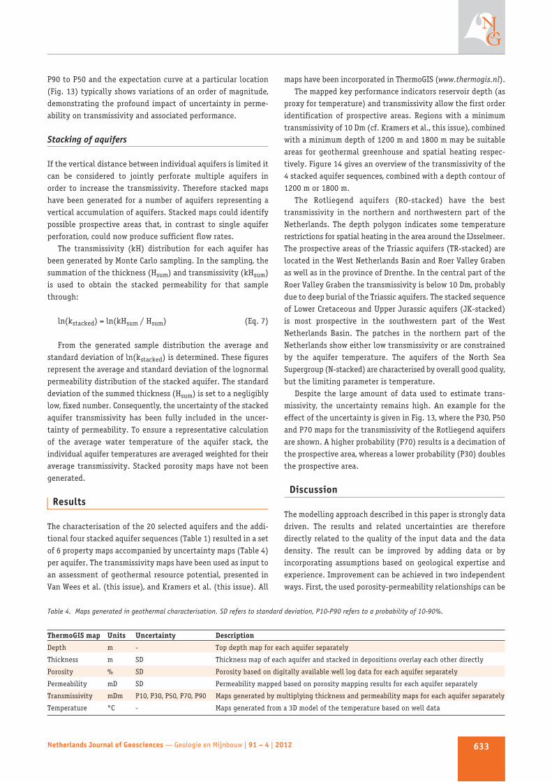
The characterisation of the 20 selected aquifers and the addi -tional four stacked aquifer sequences (Table 1) resulted in a setof 6 property maps accompanied by uncertainty maps (Table 4)per aquifer. The transmissivity maps have been used as input toan assessment of geothermal resource potential, presented inVan Wees et al. (this issue), and Kramers et al. (this issue). All
maps have been incorporated in ThermoGIS (www.thermogis.nl).The mapped key performance indicators reservoir depth (as
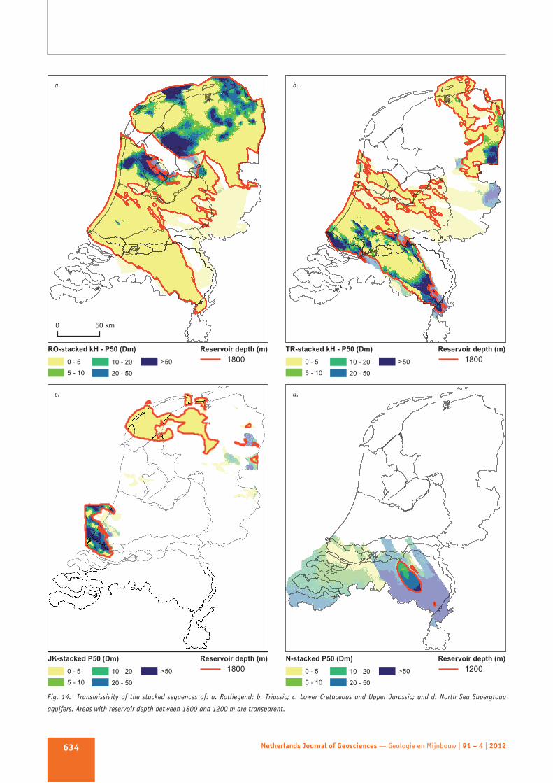
proxy for temperature) and transmissivity allow the first orderidentification of prospective areas. Regions with a minimumtransmissivity of 10 Dm (cf. Kramers et al., this issue), combinedwith a minimum depth of 1200 m and 1800 m may be suitableareas for geothermal greenhouse and spatial heating respec -tively. Figure 14 gives an overview of the transmissivity of the4 stacked aquifer sequences, combined with a depth contour of1200 m or 1800 m.
The Rotliegend aquifers (RO-stacked) have the besttransmissivity in the northern and northwestern part of theNetherlands. The depth polygon indicates some temperaturerestrictions for spatial heating in the area around the IJsselmeer.The prospective areas of the Triassic aquifers (TR-stacked) arelocated in the West Netherlands Basin and Roer Valley Grabenas well as in the province of Drenthe. In the central part of theRoer Valley Graben the transmissivity is below 10 Dm, probablydue to deep burial of the Triassic aquifers. The stacked sequenceof Lower Cretaceous and Upper Jurassic aquifers (JK-stacked)is most prospective in the southwestern part of the WestNetherlands Basin. The patches in the northern part of theNetherlands show either low transmissivity or are constrainedby the aquifer temperature. The aquifers of the North SeaSupergroup (N-stacked) are characterised by overall good quality,but the limiting parameter is temperature.
Despite the large amount of data used to estimate trans -missivity, the uncertainty remains high. An example for theeffect of the uncertainty is given in Fig. 13, where the P30, P50and P70 maps for the transmissivity of the Rotliegend aquifersare shown. A higher probability (P70) results is a decimation ofthe prospective area, whereas a lower probability (P30) doublesthe prospective area.
Discussion
The modelling approach described in this paper is strongly datadriven. The results and related uncertainties are thereforedirectly related to the quality of the input data and the datadensity. The result can be improved by adding data or byincorporating assumptions based on geological expertise andexperience. Improvement can be achieved in two independentways. First, the used porosity-permeability relationships can be
Netherlands Journal of Geosciences — Geologie en Mijnbouw | 91 – 4 | 2012 633
Table 4. Maps generated in geothermal characterisation. SD refers to standard deviation, P10-P90 refers to a probability of 10-90%.
ThermoGIS map Units Uncertainty Description
Depth m - Top depth map for each aquifer separately
Thickness m SD Thickness map of each aquifer and stacked in depositions overlay each other directly
Porosity % SD Porosity based on digitally available well log data for each aquifer separately
Permeability mD SD Permeability mapped based on porosity mapping results for each aquifer separately
Transmissivity mDm P10, P30, P50, P70, P90 Maps generated by multiplying thickness and permeability maps for each aquifer separately
Temperature °C - Maps generated from a 3D model of the temperature based on well data
Netherlands Journal of Geosciences — Geologie en Mijnbouw | 91 – 4 | 2012634
0 50 km
RO-stacked kH - P50 (Dm) Reservoir depth (m)
1800TR-stacked kH - P50 (Dm)Reservoir depth (m)
1800
JK-stacked P50 (Dm) Reservoir depth (m)
1800N-stacked P50 (Dm) Reservoir depth (m)
1200
Fig. 14. Transmissivity of the stacked sequences of: a. Rotliegend; b. Triassic; c. Lower Cretaceous and Upper Jurassic; and d. North Sea Supergroup
aquifers. Areas with reservoir depth between 1800 and 1200 m are transparent.
a. b.
c. d.
reviewed and revised in the light of data clustering and filteringin order to derive a more robust poro-perm relation. In case oflimited data available, this should be achieved by incorporatingexpert knowledge. Secondly, the spatial data distribution iscurrently based on correlation of data points expressed in avariogram. Incorporation of sedimentary facies distributions inthe modelling workflow, along with diagenesis and cementation,could also improve the model. A third improvement can beachieved by adding extra data. Besides data derived from well-logs and core measurements, incorporation of well test resultsshould have large impact on the estimation of transmissivity.
This modelling approach is developed for regional charac -terisation of reservoirs and therefore tends to oversee localheterogeneities, in particular permeability. Prospective areas canbe identified on the resulting transmissivity maps, but shouldbe examined more thoroughly in a geothermal exploration phase.
Conclusion
The presented workflow shows that regional transmissivity mapsand underlying uncertainty can be built for geothermal aquifers,taking oil and gas well data and mapping results from detailedseismic interpretation into account. We have shown that burialanomalies can have a significant effect on regional assessmentof porosity and permeability of geothermal aquifers. In general,the prospectivity of basin flanks (with few data) of invertedbasins (with most well data control) can be significantlyenhanced by incorporating burial anomalies.
Mapping of the key parameters transmissivity and tempera -ture shows favorable aquifer conditions in the northern part ofthe Netherlands for the Rotliegend aquifers, while in the westernand southern parts of the Netherlands Triassic and UpperCretaceous / Jurassic aquifers show prospectivity. Despite thehigh transmissivity of the aquifers of the North Sea Supergroup,the limited depth and therefore temperature reduces theprospective geothermal area significantly.
The results show a considerable remaining uncertainty oftransmissivity values, due to the lack of data and theheterogeneous spatial data distribution. For underexploredareas this bears a significant risk, but this can also result inmuch higher flowrates than originally expected, representingand upside in project performance. In part these uncertaintiesmay be significantly reduced by adding well test results andfacies parameters for the map interpolation in future work.
Acknowledgements
We thank H. Kombrink, the editor, and the reviewers R. Herberand R. Gaup for their constructive reviews that significantlyimproved the quality of this paper.