Page 1
Reservoir Characterization with Limited Sample Data using Geostatistics
By:
Sayyed Mojtaba Ghoraishy
Submitted to the Department of Chemical and Petroleum Engineering and the Faculty
of the Graduate School at The University of Kansas in Partial Fulfillment of the
Requirements for the Degree of Doctor of Philosophy
Chairperson: Dr. G.P. Willhite
Dissertation Committee:
Dr. Jenn-Tai Liang
Dr. Shapour Vossoughi
Dr. Anthony W. Walton
Dr. Jyun Syung Tsau
Dr. Don Green
Date Defended: October 13, 2008
Page 2
i
The dissertation committee for Sayyed Mojtaba Ghoraishy certifies
that this is the approved version of the following dissertation:
Reservoir Characterization with Limited Sample Data using Geostatistics
Chairperson: Dr. G.P. Willhite
Dissertation Committee:
Dr. Jenn-Tai Liang
Dr. Shapour Vossoughi
Dr. Anthony W. Walton
Dr. Jyun Syung Tsau
Dr. Don Green
Date Approved: December 10, 2008
Page 3
ii
Acknowledgments
The author wishes to extent his sincere gratitude to all the members of his committee Dr. G. Paul
Willhite, Dr. Green, Dr Jen Tai Liang, Dr. Jyung-Syung Tsau, Dr. Shapour Vossoughi, and Dr.
Tony Walton.
I would like to thank my fellow graduate students and officemates who made my graduate life
more fun.
The financial support of the Tertiary Oil recovery Project (TORP) is appreciated.
Lastly, and most importantly, I have to thank my wife, Leila, my son Mohammad and my
daughter Minoo for the love, encouragement, care, and support they have given me all the way.
Page 4
iii
To my wife Leila, my son Mohammad and my daughter Minoo
Page 5
iv
Abstract
The primary objective of this dissertation was to develop a systematic method to
characterize the reservoir with the limited available data. The motivation behind the study was
characterization of CO2 pilot area in the Hall Gurney Field, Lansing Kansas City Formation. The
main tool of the study was geostatistics, since only geostatistics can incorporate data from
variety of sources to estimate reservoir properties. Three different subjects in geostatistical
methods were studied, analyzed and improved.
The first part investigates the accuracy of different geostatistical methods as a function of
the available sample data. The effect of number and type of samples on conventional and
stochastical methods was studied using a synthetic reservoir. The second part of the research
focuses on developing a systematic geostatistical method to characterize a reservoir in the case of
very limited sample data. The objective in this part was the use of dynamic data, such as data
from pressure transient analysis, in geostatistical methods. In the literature review of this part
emphasis is given to those works involving the incorporation of well-test data and the use of
simulated annealing to incorporate different type of static and dynamic data. The second part
outlines a systematic procedure to estimate the reservoir properties for a CO2 pilot area in the
Lansing Kansas City formation. The third part of the thesis discusses the multiple-point
geostatistics and presents an improvement in reservoir characterization using training image
construction. Similarity distance function is used to find the most consistent and similar pattern
for to the existing data. This part of thesis presents a mathematical improvement to the existing
similarity functions.
Page 6
v
TABLE OF CONTENTS
Abstract ………………………………………………………………..................... iv
Table of Contents ………………………………………………………………....... v
List of Figures……………………………………………………………….............. x
List of Tables ……………………………………………………………….............. xix
Chapter 1. Overview ………………………………………………………………... 1
Part I - Effect of Quantity of the Sample Data on the Accuracy of
Geostatistical Methods
5
Chapter 2. Review of the Geostatistical Reservoir Characterization……………….. 6
2.1. Introduction ……………………………………………………………………. 6
2.2. Background ……………………………………………………………………. 7
2.2.1. Random Variables………………………………………… 8
2.2.2. The Random Function Concept…………………………… 11
2.2.3. Stationary Constraints…………………………………… 12
2.2.4. Covariance Function……………………………………. 14
2.2.5. Semivariograms………. ……………………………….. 16
2.2.6. Cross-Variograms……………………………………… 17
2.2.7. Mathematical Modeling of a Spatial Function…………… 18
2.3. Conventional Estimation Techniques…………………………………………. 21
2.3.1. Cell De-clustering……………………………………….. 21
2.3.2. Inverse Distance Method…………………………………. 22
2.3.3. Simple Kriging…………………………………………… 23
2.3.4. Ordinary Kriging………………………………………… 26
Page 7
vi
2.3.5. Indicator Kriging………………………………………… 27
2.3.6. Cokriging…………………………………………………. 32
2.3.7. Monte-Carlo simulation techniques……………………… 34
2.4. Review of Sequential Simulation………………………………………………. 36
2.4.1. Sequential Gaussian Simulation (SGS)……………………. 38
2.4.2. Sequential Indicator Simulation (SIS)……………………... 40
2.4.2.1. Categorical (Discrete) Variables………………….. 41
2.4.2.2. Continuous Variables……………………………... 41
Chapter 3.Investigate the Effect of Quantity of Samples on Geostatistical Methods 44
3.1. Introduction…………………………………………………………………….. 44
3.2. Case Study……………………………………………………………………… 46
3.3. Sample Data Sets………………………………………………………………. 47
3.4. Flow Simulator………………………………………………………………… 47
3.5. Methodology……………………………………………………………………. 54
3.5.1. Semivariogram Modeling………………………………….. 56
3.5.2. Ordinary Kriging………………………………………….. 61
3.5.3. Indicator Kriging………………………………………….. 67
3.5.4. Sequential Gaussian Simulation…………………………… 73
3.5.5. Sequential Indicator Kriging………………………………. 83
3.6. The Effect of Second Variable (Porosity)……………………………………… 89
3.6.1. Exponential Models (Crossplot)…………………………… 89
3.6.2. Cokriging ………………………………………………….. 96
3.7. The Effect of Quantity of Sample Data on Dynamic Data …………………. 102
Page 8
vii
Chapter 4. Conclusions…………………………………………………………... 126
Part II – Reservoir Characterization of the CO2 Pilot Area in the Hall-Gurney 128
Chapter 5. Introduction……………………………………………………………. 129
Chapter 6. Literature Review and Background……………………………………... 132
6.1. Optimization-Based Methods…………………………………………………... 136
6.2. Pilot Point Method……………………………………………………………… 140
6.3. Sequential Self-Calibration Method…………………………………………... 142
6.4. Markov Chain Monte Carlo Method………………………………………….. 144
6.5. Gradual Deformation Method………………………………………………… 147
6.6. Simulated Annealing………………………………………………………….. 149
Chapter 7. Background on Lansing Kansas City Formation……………………….. 154
7.1. Lansing Kansas City Oil Production…………………………………………… 156
7.2. Initial Reservoir Model…………………………………………………………. 161
7.2.1. Geological Model………………………………………….. 161
7.2.2. PVT Properties…………………………………………….. 167
7.2.3. History Matching the Primary and Secondary Oil
Production………………………………………………….
167
7.3. Updated Geologic Model Based on CO2I-1 Cores…………………………….. 170
7.4. CO2 Pilot area in the Hall-Gurney Field……………………………………….. 171
7.5. Field Diagnostic Activities……………………………………………………... 173
7.5.1. Short-term injection test of the CO2I-1………………….. 173
7.5.2. Shut in Colliver#18………………………………………… 174
7.5.3. Water Injection test in CO2I-1…………………………….. 174
Page 9
viii
7.5.4. Colliver-12 and Colliver-13 Production Test in June 2003. 175
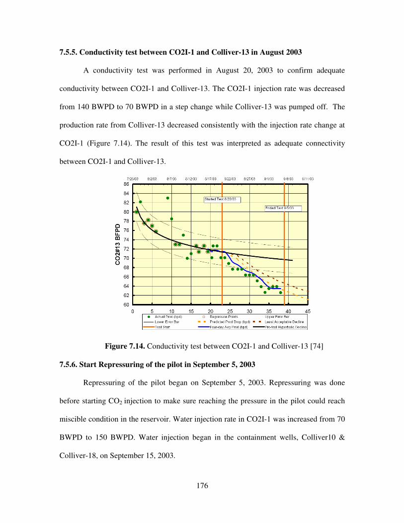
7.5.5. Conductivity test between CO2I-1 and Colliver-13……….. 176
7.5.6. Start Repressuring of the pilot in September 5, 2003…….. 176
7.6. CO2 Injection in the Hall-Gurney Field ………………………………………. 177
7.7. Modeling of Solvent (CO2) Miscible Flooding………………………………… 180
7.8. New Geological Structure and Petrophysical Properties………………………. 181
7.9. Porosity Distribution of the Geological Model………………………………… 182
7.10. Verification of the Reservoir Layering Using Descriptive Statistics……......... 183
7.11. Geostatistical Approach for Porosity Estimation……………………………... 187
7.12. Permeability Distribution……………………………………………………... 191
7.12.1. First Hypothesis: Same slope for all crossplots…………... 192
7.12.2. Second Hypothesis: Incorporation of well test data…….. 193
7.12.3. Proposed Methodology…………………………………… 194
7.13. Discriminant Analysis for Permeability and Porosity Distribution…………… 198
Chapter 8.The Flow Simulation Results…………………………………………….. 202
Chapter 9. Conclusion………………………………………………………………. 210
Part III- The Modified SIMPAT Image Processing Method for Reproducing
Geological Patterns
212
Chapter 10. Introduction……………………………………………………………. 213
Chapter 11. Background on Multiple-point (MP) Geostatistics……………………. 218
11.1. Background……………………………………………………………………. 218
11.1.1. Multi-point (MP) Statistics and Connectivity Function...... 218
11.1.2. Training Images…………………………………………... 221
11.1.3. Literature Review………………………………………… 223
Page 10
ix
Chapter 12. SIMPAT Algorithm……………………………………………………. 227
12.1. SIMPAT Algorithm………………………………………………………….... 227
12.2. Limitations of the Manhattan Distance……………………………………….. 233
Chapter 13. Modified SIMPAT Algorithm…………………………………………. 235
13.1. Normalized Cross Correlations (NCC)……………………………………….. 235
13.2. Modified SIMPAT Algorithm………………………………………………… 236
13.3. Case Studies…………………………………………………………………… 237
Chapter 14. Results and Discussions ………………………………………………. 241
14.1. The Effect of Template Size………………………………………………….. 242
14.2. Application Example for History Matching Process…………………………. 251
Chapter 15. Conclusions……………………………………………………………. 263
References………………………………………………………………………….. 265
Page 11
x
List of Figures
2.1 Cross-sectional view of a random variable ……………………………............ 10
2.2 Probability density function of a random variable …….……………………… 11
2.3 A typical covariance function for a random variable …………………………. 15
2.4 A typical semivariogram function for a random variable …………………….. 17
2.5 Basics semivariogram models with sill ………………………………………. 20
2.6 An example of cell declustering ……………………………………………… 23
2.7 Schematic illustration of probability distribution F(z) at a series of five
threshold values ……………………………………………………………….
30
2.8 Uncertainty estimation in indicator kriging …………………………………… 31
2.9 Lack of true geological continuity in kriging estimation ……………………... 35
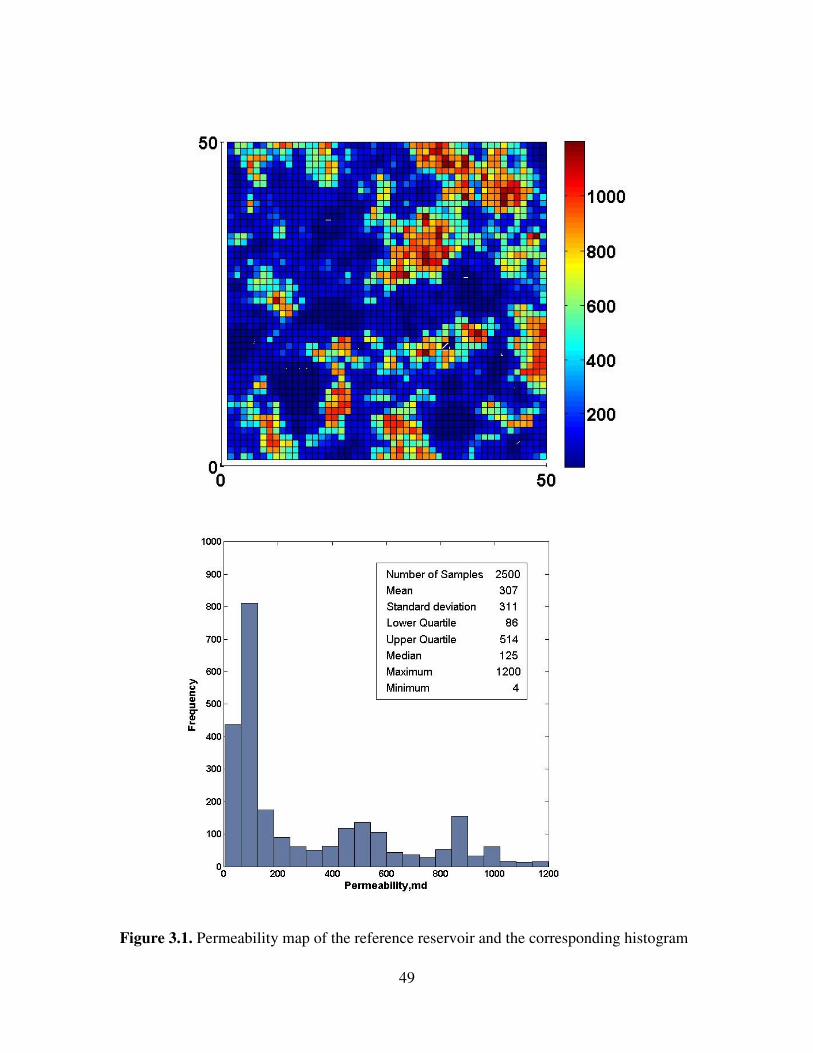
3.1 Permeability map of the reference reservoir and the corresponding histogram. 49
3.2 Porosity map of the reference reservoir and the corresponding histogram …… 50
3.3 Location of sample in 10 Acre well spacing data set …………………………. 51
3.4 Location of sample in 40 Acre well spacing data set …………………………. 52
3.5 The location of a five-spot pattern on the reference reservoir ………………… 52
3.6 Oil-water relative permeability data set used in the flow simulator …………... 53
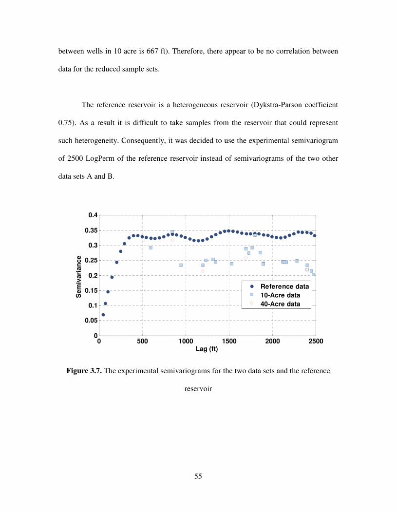
3.7 The experimental semivariograms for the two data sets and the reference
reservoir ……………………………………………………………………….
55
3.8 Experimental semivariogram of LogPerm in different direction ……………... 57
3.9 Experimental and mathematical model of semivariogram for LogPerm ……... 57
3.10 Experimental and mathematical semivariogram for lower quartile threshold… 59
Page 12
xi
3.11 Experimental and mathematical semivariogram for median threshold ………. 59
3.12 Experimental and mathematical semivariogram for upper quartile threshold ... 60
3.13 Experimental and mathematical semivariogram of the LogPerm normal score 60
3.14 Comparison of the permeability maps generated by ordinary kriging and the
reference reservoir ……………………………………………………………
62
3.15 Variance map of ordinary kriging for estimation the permeability …………… 63
3.16 Histogram of permeability maps generated by ordinary kriging ……………… 65
3.17 Location of sample data in the 40 Acre data set ………………………………. 66
3.18 The difference between LogPerm kriged and sample mean of the 40 Acre data 66
3.19 Indicator maps of the three thresholds used in IK …………………………….. 68
3.20 Histograms of indicator maps for three thresholds ……………………………. 70
3.21 Permeability maps generated by indicator kriging ……………………………. 71
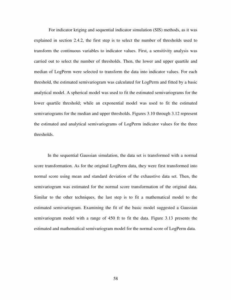
3.22 Histogram of permeability maps generated by indicator kriging ……………... 72
3.23 Comparison between semivariograms of the permeability realizations for two
data sets and the reference reservoir …………………………………………
76
3.24 SGS Permeability realizations using data set A ……………………………… 77
3.25 The difference between the permeability values of the reference reservoir and
four SGS realizations …………………………………………………………
78
3.26 The difference between the permeability values of the reference reservoir and
four SGS realizations …………………………………………………………
79
3.27 Comparison of the permeability maps generated by SGS using two data sets A
& B and the reference reservoir ……………………………………………….
80
3.28 Histograms of permeability maps shown in Figure 3.26 ……………………… 81
Page 13
xii
3.29 The difference between LogPerm sample mean and SGS simulated values for
the 40 Acre data set ………………………………………………………….
82
3.30 Comparison between semivariograms of the permeability realizations
generated by SIS using two data sets and the reference reservoir ……………
85
3.31 SIS Permeability realizations using data set A ……………………………….. 86
3.32 Comparison of the permeability maps generated by SIS using two data sets A
& B and the reference reservoir ………………………………………………
87
3.33 Histograms of permeability maps shown in Figure 3.32 …………………….. 88
3.34 Comparison of the porosity maps generated by ordinary kriging using two
data sets A & B and the reference reservoir …………………………………..
91
3.35 Crossplot of permeability and porosity for data set A ………………………… 92
3.36 Crossplot of permeability and porosity for data set B ………………………… 92
3.37 Comparison of the permeability maps generated by exponential model using
data sets A & B ……………………………………………………………….
93
3.38 Histograms of permeability maps in Figure 3.37 ……………………………... 94
3.39 Comparison between experimental semivariogram of permeability estimated
by exponential model and the reference reservoir ……………………………
95
3.40 Experimental and mathematical cross-variogram of porosity and LogPerm for
the reference reservoir ………………………………………………………..
97
3.41 Comparison of the permeability maps generated by cokriging model using
data sets A & B and the reference reservoir …………………………………..
98
3.42 Histograms of permeability maps in Figure 3.41 ……………………………... 99
Page 14
xiii
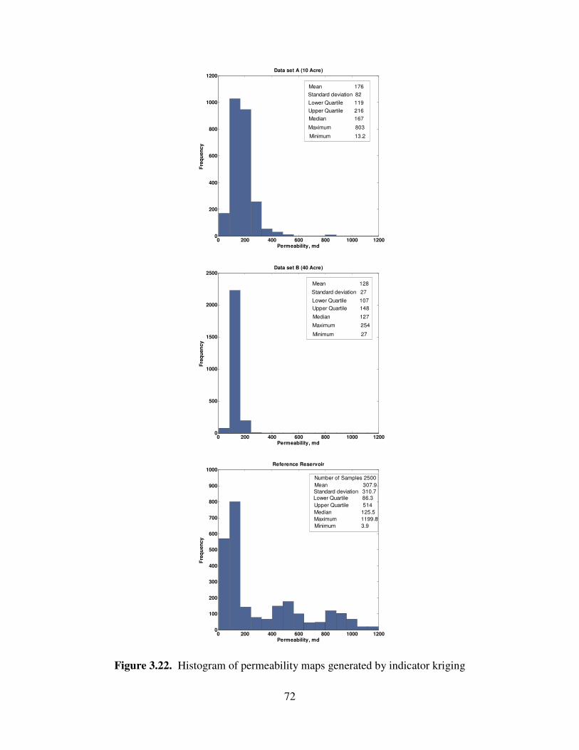
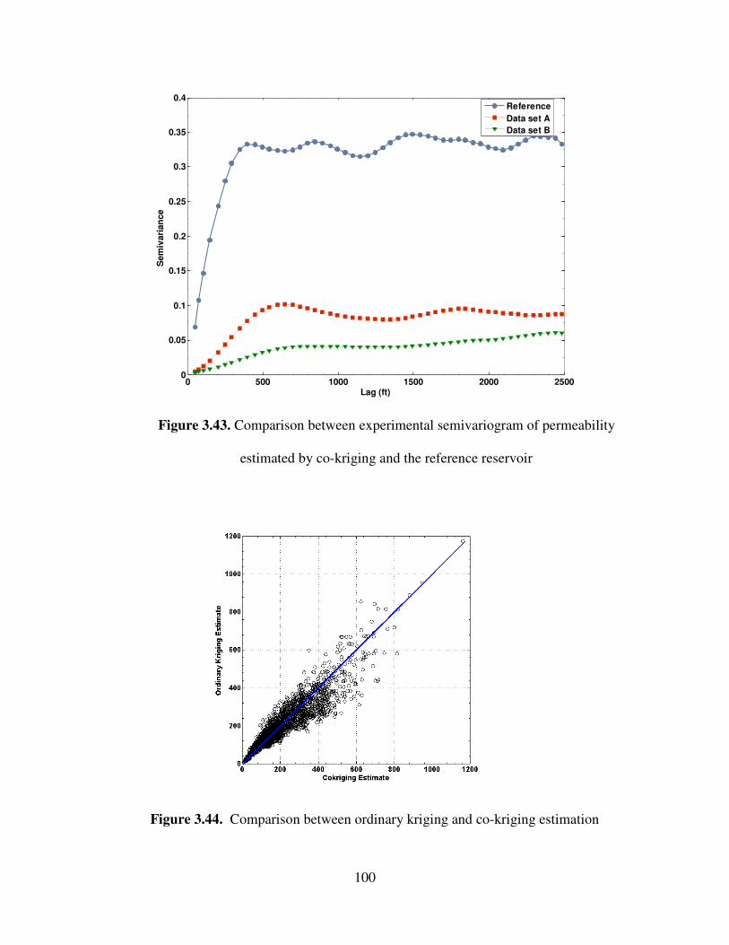
3.43 Comparison between experimental semivariogram of permeability estimated
by cokriging and the reference reservoir …………………………………….
100
3.44 Comparison between ordinary kriging and cokriging estimation …………….. 100
3.45 Comparison between ordinary kriging and cokriging estimation error variance 101
3.46 Comparison of dynamic data for ordinary kriging method using data set A …. 105
3.47 Comparison of dynamic data for ordinary kriging method using data set B …. 106
3.48 Comparison of dynamic data for indicator kriging method using data set A …. 107
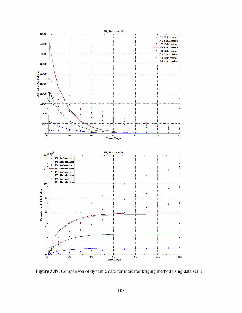
3.49 Comparison of dynamic data for indicator kriging method using data set B …. 108
3.50 Comparison of dynamic data for SGS method using data set A ……………… 109
3.51 Comparison of dynamic data for SGS method using data set B ……………… 110
3.52 Comparison of dynamic data for SIS method using data set B ………………. 111
3.53 Comparison of dynamic data for SIS method using data set B ………………. 112
3.54 Comparison of dynamic data for Crossplot method using data set A…………. 113
3.55 Comparison of dynamic data for Crossplot method using data set B…………. 114
3.56 Comparison of dynamic data for cokriging method using data set A ………… 115
3.57 Comparison of dynamic data for cokriging method using data set B ………… 116
3.58 Cumulative oil production of SGS realizations generated by data set A ……... 117
3.59 Cumulative oil production of SGS realizations generated by data set B ……... 117
3.60 Cumulative oil production of SIS realizations generated by data set A ……..... 118
3.61 Cumulative oil production of SIS realizations generated by data set A ……..... 118
3.62 Histogram of cumulative oil production after fifty days for SGS realizations
generated by data set A ………………………………………………………..
119
Page 15
xiv
3.63 Histogram of cumulative oil production after fifty days for SGS realizations
generated by data set B ………………………………………………………..
120
3.64 Histogram of cumulative oil production after fifty days for SIS realizations
generated by data set A ……………………………………………………….
121
3.65 Histogram of cumulative oil production after fifty days for SIS realizations
generated by data set B ……………………………………………………….
122
7.1 Lansing Kansas City reservoirs produced 1150 billion barrels of oil
representing 19% of total Kansas oil production ……………………………..
158
7.2 The Central Kansas Uplift in Lancing Kansas City ………………………….. 158
7.3 Stratigraphic Formation and latter nomenclature of the LKC Groups ……….. 159
7.4 The Hall-Gurney annual cumulative oil production ………………………….. 160
7.5 Crossplot of permeability-porosity for core samples in Hall-Gurney field ….. 163
7.6 The initial water saturation decreases as the permeability increases for the
same oil column height above oil-water contact ……………………………..
164
7.7 Capillary pressure curves for oomoldic limestone ……………………………. 165
7.8 History matching of oil production for Colliver lease ………………………… 169
7.9 History matching of oil production for Carter lease …………………………... 169
7.10 Permeability versus depth for Murfin Carter-Colliver CO2 I well and
Colliver#1 well ………………………………………………………………..
170
7.11 The 10-Acre CO2 pilot area in the Hall-Gurney Field ………………………… 172
7.12 Bottom hole pressures through time showing decline of reservoir pressures
following shut in Colliver-18 ............................................................................
174
Page 16
xv
7.13 The BHP response with respect to commencement of long- term water
Injection test in CO2I-1 ……………………………………………………….
175
7.14 Conductivity test between CO2I-1 and Colliver-13 …………………………... 176
7.15 Carbon dioxide injection rate in CO2I-1 ……………………………………… 178
7.16 Liquid production rate from Colliver-12 and Colliver-13 …………………….. 179
7.17 Average daily oil production rate from pilot area …………………………….. 179
7.18 A 3D view of the 8-layer geological model used in the simulation …………... 181
7.19 Available well Log data in the Hall-Gurney Field ……………………………. 182
7.20 Experimental and Analytical semivariograms of the layer 1 …………………. 189
7.21 Experimental and Analytical semivariograms of the layer 7 …………………. 189
7.22 Porosity distribution of Layer-1 ………………………………………………. 190
7.23 Porosity distribution of Layer-7 ………………………………………………. 190
7.24 The crossplot of k-Φ for all cores in the LKC formation …………………….. 192
7.25 The 3D-view of the location of the wells in the CO2 pilot area ………………. 195
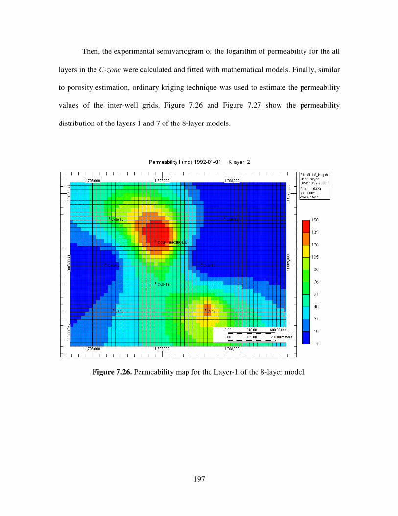
7.26 Permeability map for the Layer-1 of the 8-layer model ………………………. 197
7.27 Permeability map for the Layer-7 of the 8-layer model ………………………. 198
7.28 Discriminant function analysis for layers 1&2 ………………………………... 201
8.1 Oil-water relative permeability data set used in the flow simulator …………... 204
8.2 Comparison the simulation results and field data for Colliver 13 …………….. 205
8.3 Comparison the simulation results and field data for Colliver 12 …………….. 205
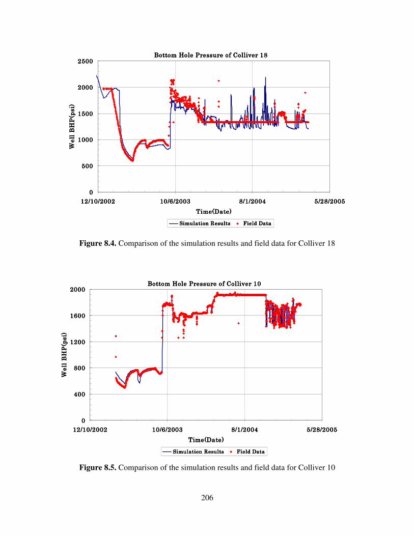
8.4 Comparison the simulation results and field data for Colliver 18 …………….. 206
8.5 Comparison the simulation results and field data for Colliver 10 …………….. 206
8.6 Comparison the simulation results and field data for CO2I-1 ………………… 207
Page 17
xvi
8.7 Comparison the simulation results and field data for Cart 2 ………………….. 207
8.8 Comparison the simulation results and field data for Cart 5 ………………….. 208
8.9 Comparison the simulation results and field Oil Production for Colliver 12 …. 208
8.10 Comparison the simulation results and field Oil Production for Colliver 13 …. 209
10.1 Stochastic realizations with same proportions of black pixels (28 %) ……….. 216
10.2 Semivariograms in horizontal direction for sisim(dashed line), elipsim(thin
line), and fluvsim(thick line) realizations…………………………………….
217
10.3 Semivariograms in vertical direction for sisim(dashed line), elipsim(thin
line), and fluvsim(thick line) realizations …………………………………….
217
11.1 Examples of 1, 2, 3, 4, and 9-point configurations ……………………………. 220
11.2 Examples of training images. All images generated using unconditional
object-based or processed-based modeling tools ……………………………..
222
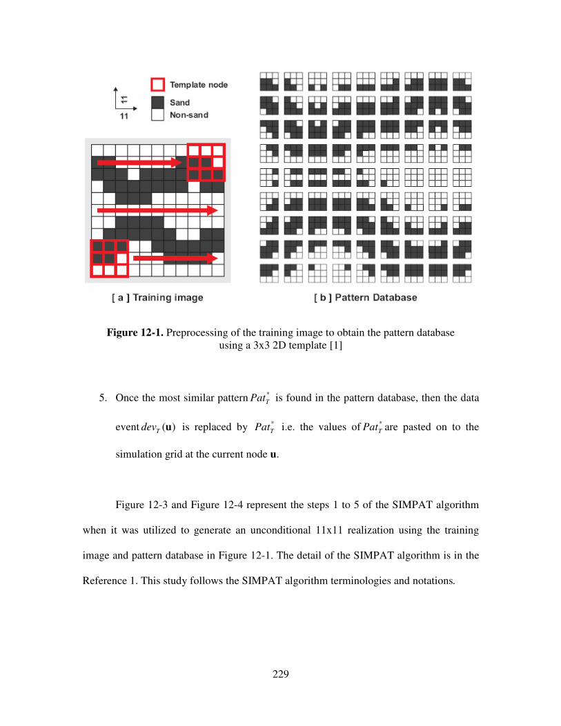
12.1 Preprocessing of the training image to obtain the pattern database using a 3x3
2D template ………………………………………………………………….
229
12.2 Application of Manhattan distance when applied to sample binary (sand/non-
sand) pattern ………………………………………………………………….
230
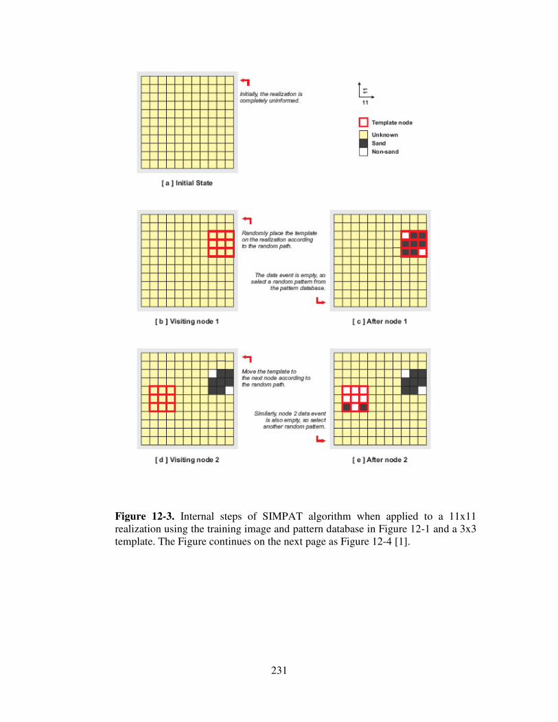
12.3 Internal steps of SIMPAT algorithm when applied to a 11x11 realization
using the training image and pattern database in Figure 12-1 and a 3x3
template. The Figure continues on the next page as Figure 12-4 …………….
231
12.4 Continuation of Figure 12.3 showing different steps of SIMPAT ……………. 232
12.5 Comparison of similarity measure distance by Manhattan and NCC
techniques for a data event on the left and candidate patterns on the right.
d<x,y> denotes the Manhattan dissimilarity distance ……………………….
234
Page 18
xvii
13.1 Training image representing a fluvial reservoir ………………………………. 239
13.2 Diagonal elliptical bodies in the training image ………………………………. 239
13.3 Training image shows four facies in the Southwest-Northeast direction …… 240
14.1 Comparison between training image 1 and simulated realizations …………… 243
14.2 Comparison between training image 2 and simulated realizations …………… 244
14.3 Comparison between training image 3 and simulated realizations …………… 245
14.4 Connectivity function of facies 1 of realizations simulated with a 30x30
template and the training image 1 …………………………………………….
246
14.5 Connectivity function of facies 1 of realizations simulated with a 30x30
template and the training image 2 …………………………………………….
246
14.6 Connectivity function of facies 1 of realizations simulated with a 30x30
template and the training image 3 ……………………………………………
247
14.7 Connectivity function of facies 1 when different template sizes used in
original and Modified SIMPAT algorithms used to generate realizations for
case study 1 ……………………………………………………………………
248
14.8 Connectivity function of facies 1 when different template sizes used in
original and Modified SIMPAT algorithms used to generate realizations for
case study 2 ……………………………………………………………………
249
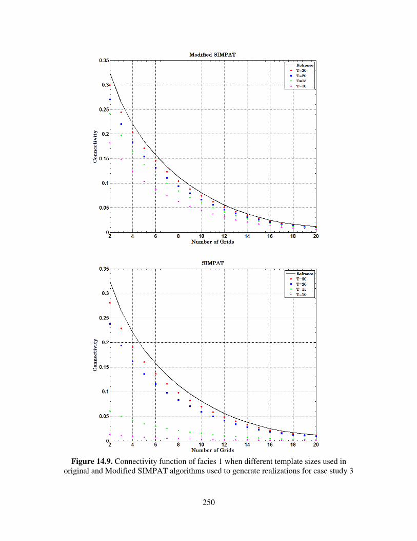
14.9 Connectivity function of facies 1 when different template sizes used in
original and Modified SIMPAT algorithms used to generate realizations for
case study 3 ……………………………………………………………………
250
14.10 The reference permeability distribution for flow simulations ………………. 253
14.11 Oil-water relative permeability data set used in the flow simulator…………. 254
Page 19
xviii
14.12 BHP’s of the four production wells obtained using fifty realizations
generated by Modified SIMPAT algorithm and the reference image ………
256
14.13 BHP’s of the four production wells obtained using fifty realizations
generated by SIMPAT algorithm and the reference image …………………
257
14.14 Water-cut of the four production wells obtained using fifty realizations
generated by Modified SIMPAT algorithm and the reference image ………
258
14.15 Water-cut of the four production wells obtained using fifty realizations
generated by SIMPAT algorithm and the reference image …………………
259
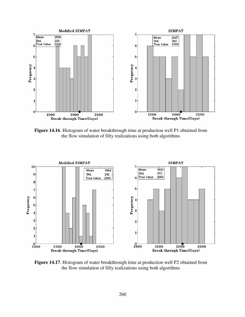
14.16 Histogram of water breakthrough time at production well P1 obtained from
the flow simulation of fifty realizations using both algorithms ……………
260
14.17 Histogram of water breakthrough time at production well P2 obtained from
the flow simulation of fifty realizations using both algorithms ……………
260
14.18 Histogram of water breakthrough time at production well P3 obtained from
the flow simulation of fifty realizations using both algorithms ……………
261
14.19 Histogram of water breakthrough time at production well P4 obtained from
the flow simulation of fifty realizations using both algorithms ……………
261
14.20 Histogram of 30% water-cut time at a production well obtained from the
flow simulation of fifty realizations using both algorithms ………………..
262
Page 20
xix
List of Tables
3.1 Model specifications for flow simulator ………………………………………. 48
3.2 RMS index for each well and the five-spot pattern …………………………… 125
7.1 The average properties of each layer in the initial geological model …………. 167
7.2 Porosity values of wells at different layers …………………………………… 183
7.3 ANOVA single for all layers of the 8-layer model …………………………… 185
7.4 t-test for porosity samples in layers 5 & 6 …………………………………….. 185
7.5 t-test for porosity samples in layers 1 & 2 …………………………………….. 186
7.6 F-test for porosity samples in layers 1 & 2 …………………………………… 186
7.7 F-test for porosity samples in layers 5 & 6 ……………………………………. 187
7.8 Intercept of permeability-porosity of the crossplots ………………………… 195
7.9 The Excel Spreadsheet for estimation the intercept of crossplot for Colliver-18 196
7.10 The Excel Spreadsheet for estimation the intercept of crossplot for CO2I-1 …. 196
7.10 Discriminant function analysis for layers 1&2 ……………………………….. 200
8.1 Model specifications for flow simulator in ECLIPSE ………………………... 204
14.1 List of parameters used in flow simulator ……………………………………. 253
Page 21
1
Chapter 1- Overview
The primary objective of this study was to develop a systematic method to
characterize the reservoir with the limited available data. The motivation behind the study
was characterization of CO2 pilot area in the Hall Gurney Field, Lansing Kansas City
Formation. The main tool of the study was geostatistics, since only geostatistics can
incorporate data from variety of sources to estimate reservoir properties. First step of the
study was to compare the different geostatistical methods and the effect of availability of
the data on the accuracy of the estimation. The second step was to propose a procedure to
estimate the reservoir properties for a CO2 pilot area in the Lansing Kansas City
formation. The proposed procedure incorporates available dynamic data to geostatistical
analysis to reduce the uncertainty. In final step, the application of multiple-point
geostatistics was studied and in the process an improvement made to reservoir
characterization using training image construction.
Reservoir modeling is a crucial step in the development and management of
petroleum reservoirs. Field development decisions made during the life of a reservoir
such as depletion strategy, number and location of production/injection wells, reservoir
pressure maintenance schemes, etc. require an accurate model of reservoir heterogeneities
and topology. Furthermore, accurate prediction of reservoir performance requires a
reservoir model that not only honors all available data but also accounts for the scale and
precision at which they are available. The data available to model a reservoir is scarce
Page 22
2
due to high acquisition costs; hence the challenge is to extract the maximum possible
reservoir information from the available data.
The data obtained from the field can be classified as static or dynamic. The static
data do not vary over time generally and are related to the intrinsic characteristics of the
rock through simple linear relationships, such as well logs, core measurements and
seismic amplitude. The dynamic data, on the other hand, do vary with time. Dynamic
data are related to the intrinsic characteristics of the rock generally through a complex,
non-linear transfer function. These include field measurements that are made regularly
throughout the life of the reservoir. Examples of this type are well-bore flowing
pressures, fluid production rates, pressure transients, fractional flow data and time-lapse
seismic data.
Geostatistics has been extensively used in reservoir characterization for a variety
reasons including its ability to successfully analyze and integrate different types of data,
provide meaningful results for model building, and quantitatively evaluate uncertainty for
risk management. Geostatistical techniques are statistical methods that develop the spatial
relationship between the sample data to model the possible values of random variables at
unsampled locations. Since its introduction to the petroleum industry almost four decades
ago, geostatistics has been increasingly used for the characterization of reservoir
properties. The most important advantage of geostatistics, that makes it attractive for
reservoir characterization, is that geostatistical techniques are numerically based. The
Page 23
3
final product of a geostatistical method is a volume of key petrophysical properties
honoring the well and seismic data.
Geostatistical methods are the focus of this thesis. Three different subjects in
geostatistical methods were studied, analyzed and improved. These subjects, although
appear unrelated in the first glance, are part of geostatistical application in reservoir
characterization. Following paragraphs briefly introduce three topic of this thesis.
The first part investigates the accuracy of different geostatistical methods as a
function of the available sample data. The effect of number and type of samples on
conventional and stochastical methods was studied using a synthetic reservoir. The topics
comes in Chapter 2 that also presents a literature review of the basic concepts of
geostatistics and different geostatistical techniques used in subsurface modeling.
The second part of the research focuses on developing a systematic geostatistical
method to characterize a reservoir in the case of very limited sample data. The objective
in this part was the use of dynamic data, such as data from pressure transient analysis, in
geostatistical methods. In the literature review of this part emphasis is given to those
works involving the incorporation of well-test data and the use of simulated annealing to
incorporate different type of static and dynamic data. The second section includes the
chapter 6 which also outlines a systematic procedure to estimate the reservoir properties
for a CO2 pilot area in the Lansing Kansas City formation.
Page 24
4
The third part of the thesis discusses the multiple-point geostatistics and presents
an improvement in reservoir characterization using training image construction. The
multiple-point geostatistics use the concept of training image for the purpose of
subsurface modeling. The image construction, in turn, relies on the concept of similarity
of available data and the patterns of a training image. Similarity distance function is used
to find the most consistent and similar pattern to the existing data. This part of thesis
presents a mathematical improvement to the existing similarity functions. Then using
examples shows its advantages to the other methods.
Page 26
6
Chapter 2
Review of the Geostatistical Reservoir Characterization
2.1. Introduction
Proper characterization of reservoir heterogeneity is a crucial requirement for
accurate prediction of reservoir performance. One of the most valuable tools for
characterization is geostatistics. Geostatistics applies statistical concepts to geological-
based phenomena and improve the modeling of the reservoir. The basis for all the
geostatistical prediction is available sample data from the reservoir. Thus it is expected
that the availability of data have effect on the accuracy of the predictions. For instance,
permeability is a key parameter to any reservoir study since it defines flow paths within
the reservoir. In a permeability characterization study, it is vital to characterize and
preserve in the model the values and their spatial patterns. The available permeability
data come from core measurements, which always represent a small proportion of the
total heterogeneity of the reservoir. Therefore, to build a reservoir geostatistical model
for permeability, it is necessary to have enough core samples to represent the real
heterogeneity of the subsurface reservoir. The objective of this part of dissertation is to
investigate the effect of the quantity of available sample data on the accuracy of
conventional and stochastic geostatistical methods in predicting the permeability
distribution.
In this chapter, a brief review of basic geostatistical concepts and methods is
presented. The methods is based on all theories, equations and ideas in the existing
Page 27
7
literature [11,18,34,37]. In chapter three, four geostatistical methods (selected based on
performance and ease of implementation), were applied to investigate the effect of
number of the available data on the accuracy of prediction.
2.2. Background
This section briefly reviews the fundamentals of geostatistics that are essential in
understanding this study. For the deeper understanding of subject matter and the
mathematics behind it, however, readers are referred to existing literature[11,18,34,37].
2.2.1. Random Variables
A random variable is a variable with values that are randomly generated
according to a probabilistic mechanism. The throwing of a die, for instance, produces
random values from the set {1, 2, 3, 4, 5, 6}.
Random variables are seen in a wide variety of scientific and engineering
disciplines. In meteorology, for example, temperature and pressure that are collected at
some stations are used to model the weather pattern. In this case, temperature and
pressure can be regarded as random variables. In geology and petroleum engineering, the
estimate of variation of subsurface properties such as formation thickness, permeability,
and porosity are regarded as random variables.
Mathematically, a numeric sequence is said to be statistically random when it
contains no recognizable patterns or regularities; sequences such as the results of an ideal
Page 28
8
die roll. Some, such as the annual amount of rainfall, are time dependent; others, such as
the thickness of geological formation are invariant at the human scale of the time. The
accurate characterization of a random variable is an expensive and time-consuming
problem. Commonly, random variables are known only through a scattered set of
observations (table function). In statistical jargon, the selected observation is called
samples.
Random variables at specific location or time have a degree of uncertainty, even if
the observations have been carefully taken to minimize measurement error. The value of
a random variable at unsampled locations is uncertain, and no method has been devised
yet to yield error-free estimates. Figure 2.1 is a cross-section based on two sample
elements at locations A and B, where the random variable is known. Here, any surface is
a possible description of the real random variable at the unsampled locations. The four
alternatives presented in Figure 2.1 are a small subset of all possible answers. For some
arbitrary location, such as C, a table can be prepared containing all the estimated values
at that location. The minimum and maximum values in the table define the interval which
encloses all likely answers to the value of the parameter at location C. A tabulation of
events and their associated probability of occurrence corresponds to the statistical
concept of a probability density function. Figure 2.2 represents a hypothetical probability
density function for all likely values of spatial function at some arbitrary unsampled
location. Based on the probability density function at location C, one value of the random
variable in Figure 2.1 is more probable than the other values.
Page 29
9
In general, the variation in the outcomes of a random variable is presented by an
informative short description rather than listing all its possible outcomes. The average of
all possible outcomes of a random variable weighted by their probability of occurrence is
the mean of sample. The mean is the central value of all outcomes. The weighted
average of the squares of the differences between the outcomes and the mean is the
variance. The variance becomes larger when the differences increase. The standard
deviation is the square root of the variance. Thus, variance and the standard deviation are
measures of the dispersion of the outcomes relative to the mean value. The standard
deviation of Figure 2.2 is a measure of the uncertainty as the true value of the random
variable at point C in Figure 2.1. A small standard deviation indicates the outcomes are
clustered tightly around the central value (mean) over relatively narrow range of
possibilities.
Throughout this dissertation, the uppercase letters, such as Z, denote a random
variable while the lower case letters, such as z, denote the outcome values. Also, the set
of possible outcomes that a random variable might take is denoted by )(),...,1( nzz and
the outcomes that are actually observed are denoted by nzz ,...,1 .
Page 30
10
LocationLocationLocationLocation
Random
Variable
Random
Variable
Random
Variable
Random
Variable
A
B
C
LocationLocationLocationLocation
Random
Variable
Random
Variable
Random
Variable
Random
Variable
A
B
C
LocationLocationLocationLocation
Random
Variable
Random
Variable
Random
Variable
Random
Variable
A
B
C
LocationLocationLocationLocation
Random
Variable
Random
Variable
Random
Variable
Random
Variable
A
B
C
Figure 2.1. Cross-sectional view of a random variable. The random variable is known at
locations A and B, but is not known at other locations, such as C.
Page 31
11
Figure 2.2 Probability density function of a random variable at a location not considered
in the sampling process, such as location C in Figure 2.1
2.2.2. The Random Function Concept
A random function is a function that its independent variables are random
variables. In other words a random function performs a set of mathematical operation on
the random variables.
For instance, in the throwing a single die example, a random function can be
defined as the set of values generated by throwing a die and doubling the outcomes. If
the random variable (RV) at location u is denoted by Z(u), a random function (RF) is a
set of RV’s defined over some field such as porosity and formation thickness. Just as a
random variable Z(u) is characterized by its conditional distribution function (cdf), a RF
Page 32
12
is characterized by the set of all its N-variate cdfs for any number N and any choice of the
N locations ui, i=1,…,N within the study area A:
})(,...,)({Prob),...,;,...,( 1111 NNnn zZzZzzF ≤≤= uuuu (2.1)
Similar to the univariate cdf of the RV Z(u), that is used to characterize uncertainty about
the value z(u), the multivariate cdf in Eq.(2.1) is used to characterize joint uncertainty
about the N values z(u1),…, z(uN). Particularly, this is important when using the
bivariate (N=2) cdf of any two RVs Z(u1), Z(u2). In fact, conventional geostatistical
procedures are restricted to univariate (F(u,z)) and bivariate distributions defined as:
})(,)({Prob),;,( 22112121 zZzZzzF ≤≤= uuuu (2.2)
2.2.3. Stationary Constraints
The assumption of stationarity is an essential assumption in geostatistical
analysis. Stationarity means that a random function has certain properties such as mean or
covariance that are constant everywhere in the region of interest. The decision of the
stationarity, in other words, is the decision of which data should be picked up from region
of interest for the analysis. Stationarity is divided into categories; the first order and the
second order.
Mathematically, the first order of stationarity can be written as
[ ] [ ])()( LuZfuZfrrr
+= (2.3)
Where []f is any function of a random variable, )(ur
and )( Lurr
+ define the two locations
of the random variable. The most commonly used random function in Eq.(2.3) is the
expected value. The expected value of the variable itself is an arithmetic mean. That
Page 33
13
means that arithmetic means of random variables across the region are the same. Using
expected value, Eq.(2.3) is written as:
[ ] [ ])()( LuZEuZErrr
+= (2.4)
That is, the expected value of a random variable at )(ur
is the same as the expected value
of a random variable Lr
lag distance away. The value of Lr
can vary from zero to the
maximum distance between variables within the region of interest. If the region of
interest divided into small subregions, and within each subregions the mean or expected
value of samples are calculated (assuming that adequate numbers of samples are present
within each subregion), those means should remain fairly close to each other assuming
first order of stationarity. If the means vary significantly, the assumption of stationarity
may not hold. Also the first order of stationarity may not hold if the sampled data have a
strong trend.
The second order of stationarity can be mathematically defined as:
[ ] [ ])(),()(),( 2211 LuZuZfLuZuZfrrrrrr
+=+ (2.5)
This relationship indicates that any function of two random variables located L distance
apart is independent of the location and is a function of only the distance and the
direction between the two locations. The arrows over the u and L indicate that locations
can be treated in terms of vectors rather than distances.
In practice, covariance can be used as one of the functions that relate two
variables located a certain distance and direction apart. In other words,
[ ] [ ])(),()(),( 2211 LuZuZCLuZuZCrrrrrr
+=+ (2.6)
Page 34
14
That is, the covariance within the region of stationarity is function of only the vector L,
not the variable itself. This is an important assumption that implies by knowing the
distance and direction between any two points, the covariance between the random
variables at these two points can be estimated without knowing the actual random
variable at those locations.
2.2.4. Covariance Function
Computational procedures used to present the statistics of a single random
variable can be extended to calculate the joint variability of pair random variables. In
bivariate statistics, the covariance function is a tool that is employed to present the joint
statistics of two RVs. For two random variables )(),( 21 uu ZZ , the covariance function at
two locations u1 and u2 is defined as:
)}]()()}{()([{),( 222 uuuuuu 111 µµ −−= ZZEC (2.7)
where E is the expected value or mean of the expression, )()( 21 uu µµ and are the means
of Z at u1 and u2 respectively. Assuming first order stationarity that the mean of the
random variable is constant everywhere, Eq.(2.7) can be rewritten as:
])}()([{),( 2
22 µ−= uuuu 11 ZZEC (2.8)
Experimental covariance can be calculated as:
2)(
1
)(
1
)(1
)()()(
1)(
−+= ∑∑
==
Ln
i
iii
Ln
i
i uzn
LuzuzLn
Lc
rr
rrrrr
r (2.9)
Where )(Lnr
is the number of pairs at vector distance L; )( iuzr
and )( Luz i
rr+ are values of
the variable at locations iur
and Lu i
rr+ respectively, and n is the total number of sample
Page 35
15
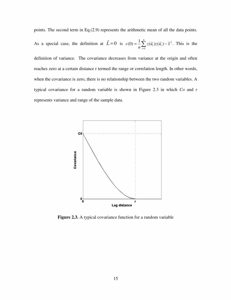
points. The second term in Eq.(2.9) represents the arithmetic mean of all the data points.
As a special case, the definition at 0=Lr
is 2
1
)()(1
)0( xuzuzn
c i
n
i
i −= ∑=
rr. This is the
definition of variance. The covariance decreases from variance at the origin and often
reaches zero at a certain distance r termed the range or correlation length. In other words,
when the covariance is zero, there is no relationship between the two random variables. A
typical covariance for a random variable is shown in Figure 2.3 in which Co and r
represents variance and range of the sample data.
Figure 2.3. A typical covariance function for a random variable
Page 36
16
2.2.5. Semivariograms
The semivariogram is the most commonly used geostatistical technique for
describing the spatial relationship of random variables. Mathematically, semivariogram
is defined as:
[ ] [ ]{ }( )
[ ]{ }( )2
22
)LZ()Z(E
)LZ()Z( E2
1)()(
2
1)(
r
rrr
+−
−+−=−+=
uu
uuuu ZLZL σγ (2.10)
It is half of the variance of the difference between the two values of a random variable
located L distance apart. Assuming the first order stationarity the second term on the
right side of Eq.(2.10) is equal zero. As a result, the semivariogram is rewritten as:
])}()([{2
1)(
2uu ZLZEL −+=
rrγ (2.11)
Under the decision of stationarity the covariance and semivariogram functions are related
tools for characterizing two-point correlation:
)()0()( LCLCrr
γ−= (2.12)
where C(0) is the covariance function at L=0. Eq.(2.12) indicates that the difference
between the two function increases as the distance increases. Experimentally, the
semivariogram for lag distance Lr
is defined as the average squared difference of values
separated approximately by Lr
:
2)(
1
)]()([)(
1)( uu
rrrr
rr
zLzLn
LLn
i
∑=
−+=γ (2.13)
where )(Lnr
is the number of pairs at vector distance Lr
; )(uz and )( Lzr
+u are the data
values for the ith pair located Lr
lag distance apart. Semivariogram can be calculated for
several directions in 3D space. The semivariogram increases from zero at the origin and
Page 37
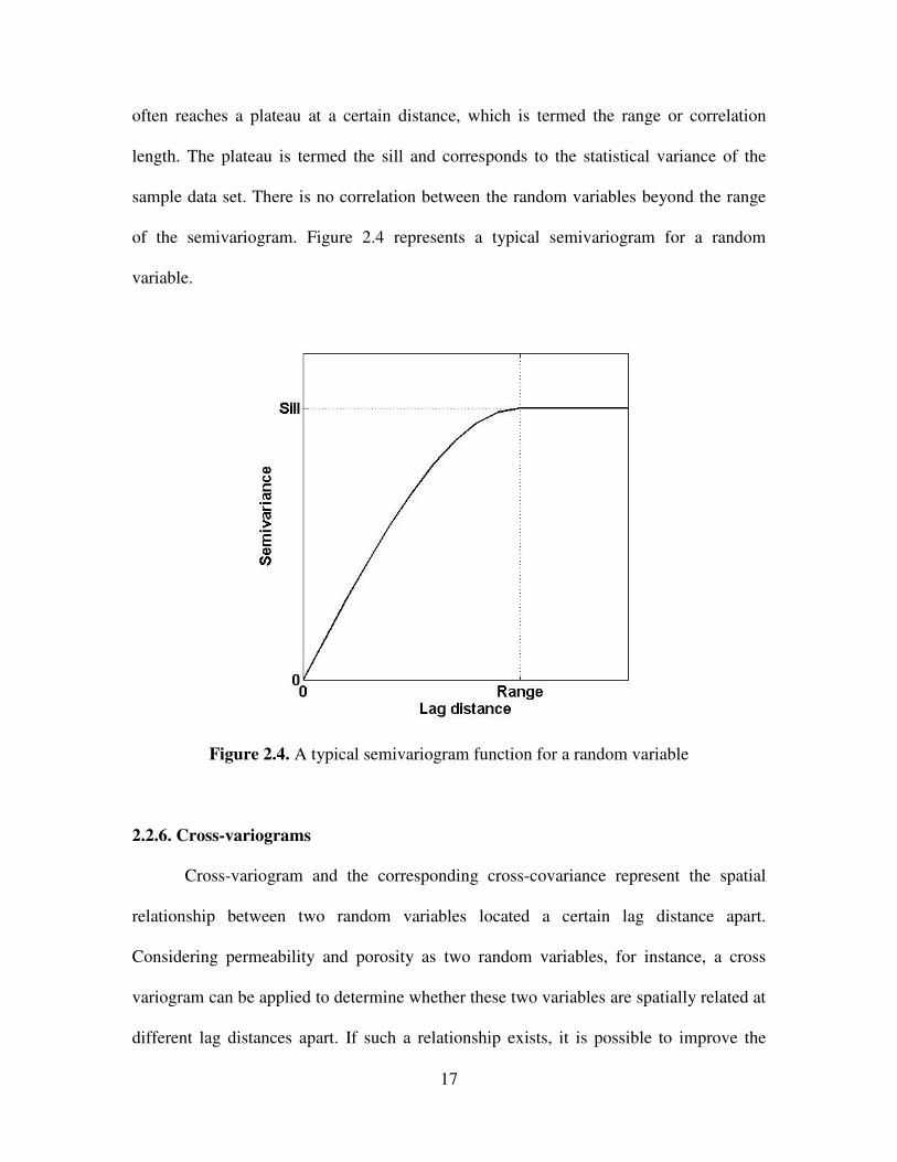
17
often reaches a plateau at a certain distance, which is termed the range or correlation
length. The plateau is termed the sill and corresponds to the statistical variance of the
sample data set. There is no correlation between the random variables beyond the range
of the semivariogram. Figure 2.4 represents a typical semivariogram for a random
variable.
Figure 2.4. A typical semivariogram function for a random variable
2.2.6. Cross-variograms
Cross-variogram and the corresponding cross-covariance represent the spatial
relationship between two random variables located a certain lag distance apart.
Considering permeability and porosity as two random variables, for instance, a cross
variogram can be applied to determine whether these two variables are spatially related at
different lag distances apart. If such a relationship exists, it is possible to improve the
Page 38
18
estimation of a random variable at the unsampled location. Mathematically, the cross
variogram is defined as:
)}]()()}{()([{2
1)( 2211 LZZLZZELc
rrr+−+−= uuuuγ (2.14)
where E is the expected value, and Z1, Z2 are RVs representing the permeability and
porosity respectively. Experimentally, the cross-variogram is estimates as:
)]()([)]()([)(2
1)( 221
)(
1
1 LzzLzzLn
LLn
i
c
rrr
rr
+−+−= ∑=
uuuuγ (2.15)
Where )(Lnr
is the number of pairs at vector distance Lr
; and z1, z2 are the values of two
properties at locations that are Lr
distance apart. Obviously, the estimation of cross
experimental cross variogram requires that both variable values be available at different
locations.
2.2.7. Mathematical Modeling of a Spatial Function
The primary purpose in estimating a semivariogram or covariance is to use them
to estimate values of the random variable at unsampled locations. However, these spatial
functions are only available at limited lag distances. There are desired lag-distances for
which the corresponding semivariogram value is not available. Hence, it is necessary to
develop a mathematical model that could be used for any lag distance in the estimation
process. Such a mathematical model must match closely with the estimated
semivariogram at available lag distances.
For the mathematical modeling of an experimental semivariogram, two
requirements must be considered. The first is to use of the minimum number of
Page 39
19
parameters in the mathematical model to make it simple. In other words, the most
important features of an estimated variogram must be captured with as a few parameters
as possible. That means the model does not need to pass through every estimated
semivariogram value. The second requirement is the condition of positive definiteness
[34]. In other words, Any model used to match the experimental semivariogram or
covariance data should satisfy this requirement which ensures a unique solution for the
estimation procedure.
There are several models in the literature that satisfy the above requirement.
Figure 2.5 represents three transitions semivariogram models. The choice of
mathematical models for a matching process depends on the behavior of the experimental
data near the origin. For instance, if the underlying phenomenon is continuous, the
estimated spatial function will likely show a parabolic behavior near the origin, and the
Gaussian semivariogram model will usually provide the best fit for this case. When there
is discontinuity among the estimated semivariogram values near the origin, a nugget
model is considered for matching process. The nugget model indicates total lack of
information with respect to the spatial relationship.
Nugget signifies the lack of quantitative information about the random variable
under the study. There are two reasons for observing nugget effect discontinuity. First,
the shortest distance at which the sample pairs are available may be greater than the range
of the variogram. The second is the measurement errors that add uncertainty in the
Page 40
20
estimation process. Figure 2.5 indicates a Nugget model. In the figure, the abrupt increase
of semivariogram values from 0 to C0 shows the nugget effect.
Figure 2.5. Basics semivariogram models with sill
In addition, a linear combination of any of the four semivariogram mathematical
models described above could be used to match a given experimental semivariogram.
Mathematically, these combinations are shown as follows:
∑+=
N
i
ii LaaL )()( 0
rrγγ (2.16)
where 0a represents the nugget effect and sai ' show the contribution of other
semivariogram model.
Page 41
21
2.3. Conventional Estimation Techniques
In principle, all estimation techniques assume that the value at the unsampled
location is estimated by
)()(1
0
* ∑=
=
n
i
ii uZuZrr
λ (2.17)
Where )( 0
*uZr
is the estimated value at the unsampled location, )( iuZr
is the value at
neighboring location iur
, and iλ is the weight assigned to any neighboring value )( iuZr
.
That is to say the estimated value is a weighted average of the neighboring values. The
goal in the estimation procedure is to calculate the weights assigned to the individual
neighboring points.
Different techniques have been proposed for the estimation based on finding the
weights to the points in the neighborhood region [17,21,34,35,46]. The neighborhood
region defines the neighboring sample points used in estimating values at the unsampled
location. In the following sections some of these methods will be reviewed.
2.3.1. Cell De-clustering
In practice, sample data are rarely collected to represent statistical properties. For
instance, wells are often drilled in areas with greater probability of good reservoir quality
not with purpose of finding the permeability at the location. This is the same for core
measurements. In this situation, the sample data are clustered in some area.
Page 42
22
In the cell de-clustering approach, the entire area is divided into rectangular
regions called cells. Each sample receives a weight inversely proportional to the number
of samples that fall within the same cell. As a result, the clustered samples generally
receive lower weights. This is because the cells in which they are located also contain
several other samples. Figure 2.6 shows a grid of cells superimposed on a number of
clustered samples. The dashed lines show the boundaries of cells. The two cells in the
north contain only one sample; so both of these samples receive a weight of one. On the
other hand, the southwestern cell contains two samples, both of which receive a weight of
1/2. Also, the southeastern cell contains eight samples that receive a weight of 1/8. The
cell de-clustering method can be viewed as a two-step procedure. In the first step, sample
data are used to calculate the mean value within the cells, and then the mean of these
samples is used for calculation at unsampled locations.
2.3.2. Inverse Distance Method
Inverse distance methods estimate the value of the random variable at an
unsampled location by assigning a larger weight to closest sample and a smaller weight to
the farthest one. This is possible by weighting each sample in a data set inversely
proportional to its distance from unsampled locations. Mathematically, it is defined as
follows:
∑
∑=
=n
p
i
n
i
ip
i
d
uZd
uZ
1
1
0
*
1
)(1
)(
r
r (2.18)
Page 43
23
where di is the distances from each of the n sample locations to the point being estimated
and p is an arbitrary constant. Traditionally, the most common choice for p is 2 since it
results in fewer calculations.
Figure 2.6. An example of cell declustering
2.3.3. Simple Kriging
Simple kriging starts with assumption that the value of a random variable at an
unsampled location could be estimated as follows:
)()(1
00
* ∑=
+=
n
i
ii uZuZrr
λλ (2.19)
n=1 n=1
n=2 n=8
Page 44
24
The value of λi is estimated by using MUVE (Minimum Variance Unbiased Estimate)
criterion. An unbiased condition requires that:
0))()(( 00
*=− uZuZE
rr (2.20)
Substituting )( 0
*uZr
from Eq.(2.19),
)]([)]([ 0
1
0 uZEuZEn
i
ii
rr=+∑
=
λλ (2.21)
By assuming first order stationarity condition, )]([)]([ 0uZEuZE i
rr= it can be written
∑−=
n
im1
0 )1( λλ (2.22)
In addition to unbiased criterion in Eq.(2.20), the condition of minimum variance must
also be satisfied. Mathematically, weights ( )iλ are chosen in a manner that
)]()([ 00
*2uZuZrr
−σ is minimized. The result of this condition is as follows:
njiforuuCuuC iji
n
i
i ,...,1,),(),( 0 ==∑rrrr
λ (2.23)
Where ji uuCrr
,( ) is the covariance value between points located at iur
and jur
respectively,
and 0,( uuC i
rr) is the covariance between the sampled location, iu
r, and the unsampled
location 0ur
. The covariance values are obtained based on the spatial model. In matrix
form, Eq.(2.23) can be written as
=
),(
.
.
.
),(
.
.
.
),(...),(
..
..
..
),(...),(
0
011
1
1111
uuC
uuC
uuCuuC
uuCuuC
nnnnn
n
λ
λ
(2.24)
Page 45
25
Rearranging the above equation in compact matrix, the weight matrix is calculated as
follows:
cC1−
=Λ (2.25)
Eq.(2.25) states that the weights assigned to the samples are directly proportional to c
and inversely proportional to C , where c represents the covariance between the sample
point and the unsampled location. The stronger the spatial relationship between the
sample point and the unsampled location, the larger is the value of ),( 0uuC i
rr. As a result,
the weight assigned to the sample point at iur
is greater. On the other hand, C represents
the covariance among the sampled points. If a particular sample point at ui is very close to
the surrounding sample points (i.e. clustered sampled), C will be large and 1−
C will be
small, and as a result the weight assigned to sample point will be reduced. If sample
points are clustered together, they do not receive large weights because they do not
provide independent information on an individual basis.
In summary, the weight assigned to an individual sample is dependent on two
factors. One is its spatial relationship to the unsampled location. The stronger the
relationship, the larger is the assigned value. The second factor is the sample point’s
spatial relationship to other sample point. The stronger the relationship, the less
independent information that point can provide. In addition to the estimation, error
variance associated with the estimation can be calculated as follows:
),(),(ˆ0
1
00
2uuCuuC i
n
iE
rrrr∑−= λσ (2.26)
Page 46
26
By examining Eq.(2.26) it is observed that the maximum value of the error variance
is ),( 00 uuCrr
(data variance). It means that in the absence of spatial information, uncertainty
with respect to estimation is represented by the variance of the data. As spatial
relationship information becomes available, error variance is reduced.
2.3.4. Ordinary Kriging
In the simple kriging procedure, it is assumed that the mean value m(u) is known.
In practice, however, the true global mean is rarely known unless it is assumed that the
sample mean is the same as global mean. Besides, the local mean within the search
neighborhood may vary over the region of interest. As a result, the assumption of first
order stationarity may not be strictly valid for the estimation process. The ordinary
kriging method was developed to overcome this problem by redefining the estimation
equation.
Considering Eq.(2.20), and )()]([)]([ 00 umuZEuZE i
rrr== , where )( 0um
rrepresents
the mean within the search neighborhood of location 0ur
, then Eq.(2.22) could be written
in the following form:
∑−=
n
ium1
00 )1)(( λλr
(2.27)
It is possible to force 0λ to be zero by assuming,
∑ =
n
i
1
1λ (2.28)
Then, the estimation equation is written as:
Page 47
27
)()(1
0
* ∑=
=
n
i
ii uZuZrr
λ (2.29)
The necessity of having the mean value is also eliminated by forcing 0λ to be zero.
Furthermore, using this constraint in Eq.(2.28) (the minimum variance criterion) results
in:
njiforuuCuuC iji
n
i
i ,...,1,),(),( 0 ==+∑rrrr
µλ (2.30)
Where µ is called a Lagrange parameter, and C represents the covariance. In matrix form,
Eq.(2.30) is written as:
01.11
),(),(
..
..
),(...),(
1
111
nnn
n
uuCuuC
uuCuuC
µ
λ
λ
n
.
.
1
=
1
),(
.
.
),(
0
01
uuC
uuC
n
(2.31)
Once λi is calculated, the error variance can be estimated by
µλσ −−= ∑ ),(),(ˆ0
1
00
2uuCuuC i
n
iE
rrrr (2.32)
2.3.5 Indicator Kriging
The main idea behind the indicator kriging is to code all of the data in a common
format as probability values. The main advantage of this approach is simplified data
integration due to the common probability coding. The comparative performance of
indicator methods has been studied extensively by Goovarets [33].
Page 48
28
An indicator variable is essentially a binary variable which takes the values 1 and
0 only. Typically such variable denotes presence or absence of a property. For a
continuous variable, the equation for an indicator transform is written as:
>
≤=
tj
tj
tj zuZif
zuZifzuI
)(0
)(1),( r
rr
(2.33)
Where ),( tj zuIr is the indicator value, )( juZ
r is the value of the random variable at jur
, and
tz is the threshold value. Depending on the value of )( juZr the indicator value could take
either a value of one or zero. Similar to a continuous variable, an equation for a discrete
variable is written as:
≠
==
tj
tj
tj KuKif
KuKifKuI
)(0
)(1),( r
rr
(2.34)
tK represents a threshold value. Depending on whether the sample value is equal or not
equal to the threshold value, the indicator variable can take either a value of zero or one.
For both continuous and discrete variables it is helpful to understand the indicator
variable in terms of the confidence in a sample value. If there is 100% confidence about a
sample, indicator values are defined in terms of zero or one. On the other hand, a value
between zero and one represents the uncertainty in the sampled value. This provides
flexibility in assigning probability values when information about particular sample point
is incomplete.
The goal of indicator kriging is to directly estimate the distribution of uncertainty
Fz(u) at unsampled location u. The cumulative distribution function is estimated at a
Page 49
29
series of threshold values: zk,k=1,…,K. For instance, Figure 2.7 shows probability values
at five threshold (K=5) values that provide a distribution of uncertainty at unsampled
location u. The probability values are evaluated by coding the data as indicator value or
probability values. The correct selection of the threshold values zk for the indicator
kriging is important. Selection of too many threshold values makes the inference and
computation needlessly tedious and expensive. On the other hand, with too few
thresholds the distribution details are lost.
After selecting the threshold values, the indicator variogram is calculated and
fitted by a mathematical model for each threshold value. Once the indicator values at
each threshold are defined, the next step is to estimate the spatial relationships or
semivariograms. The number of semivariograms depends on the number of thresholds.
For a continuous variable, such as permeability, if high permeability values exhibit
different continuity than low permeability values, indicator approach provides the
flexibility to model different levels of permeability with different semivariograms.
Page 50
30
Figure 2.7. Schematic illustration of probability distribution F(z) at a series of five
threshold values, zk, k=1,...,5 [35]
The final step is to estimate an indicator value at unsampled locations. The
approach is the same as the one for conventional kriging, except the kriging procedure is
repeated at each threshold. For ordinary kriging the equation is:
∑=
+=
n
j
tjjt zuIzuI1
00
* ),(),(rr
λλ (2.35)
And for simple kriging the equation is:
∑=
=
n
j
tjjt zuIzuI1
0
* ),(),(rr
λ (2.36)
Page 51
31
Because the weights assigned to sample points fall between zero and one, and the
indicator values are between zero and one, the estimate from both equation fall between
zero and one. After all unsampled points are visited; the indicator value for each
threshold at each location is available. The estimate depends on whether indicator kriging
used for continuous or discrete variables. Figure 2.8 represents possible estimates that
could be obtained for continuous variables. For example, location (a) for continuous
variable indicates that there is 20% probability that the value at that location is less than
the first threshold.
A similar explanation could be given for the other thresholds. By examining the
probabilities for the location (b) in Figure 2.8, the probability of a sample value occurring
between the second and third thresholds is 0.9-0.2=0.7. This high probability shows that
the value falls within that interval.
Figure 2.8. Uncertainty estimation in indicator kriging
0.1
0.2
0.9
0.9
0.8
0.6
0.2
(a)
0.95
(b)
Page 52
32
2.3.6. Co-kriging
The term co-kriging is reserved for linear regression that correlates data that is
defined with different attributes. Basically, the goal in co-kriging is to improve the
estimate and reduce the uncertainty in the kriging estimation with the help of spatial
information available from other variables. The implicit assumption in the process is the
variable of interest and the other variables are spatially related to each other. For instance,
to improve reservoir description, permeability can be estimated by using porosity data.
This could be beneficial to permeability estimation since typically, a few wells are cored
but almost all wells are logged. By establishing a spatial relationship between porosity
and permeability data, the estimation of permeability at unsampled location could be
improved by the surrounding porosity data.
The limitation of co-kriging is that the variables must be linearly related to each
other. Therefore, it is critical to check the relationship between the variable of interest
(principle variable) and the supporting variables (covariables). Furthermore, the
application of co-kriging requires a substantial spatial modeling and additional
computational effort compared to an ordinary kriging system.
Mathematically, if n and m are the number of samples of the principal variables
and covariable Y respectively, then
)()()(1
*
1
*
0
* ∑∑==
+=
m
k
YY
n
i
izk
kiuYuZuZrrr
λλ (2.37)
Page 53
33
Where iz
*λ is the weight assigned to the sample )( iuZ
rand
kY*
λ is the weight assigned to
the sample )(kYuY
r.
From Eq.(2.37) and the unbiased condition, 0))()(( 00
*=− uZuZE
rr we can write
011
=−+ ∑∑==
z
n
k
YY
n
i
Zx mmmki
λλ (2.38)
Where zm and Ym are the expected values of the Z and Y variables, respectively.
The following equations are written to satisfy the unbiased condition,
11
=∑=
n
i
Z iλ 1
1
=∑=
n
i
Yiλ (2.39)
Finally, by minimizing the variance, the following equation in matrix form can be solved
to calculate the weights, iλ
001...10...0
000...01...1
10),(...),(),(...),(
........................
10),(...),(),(...),(
01),(...),(),(...),(
...................
01),(...),(),(...),(
1111
111111
11
111111
YmmYYYYYYZnCYZC
YmYYYYYYZCYZC
YZCYZCZZZXZZ
YZCYZCZZZZZZ
uuCuuCuuCuuC
uuCuuCuuCuuC
uuCuuCuuCuuC
uuCuuCuuCuuC
mm
n
mnnnnn
mn
rrrrrrrr
rrrrrrrr
rrrrrrrr
rrrrrrrr
Y
Z
Yn
Y
Zn
Z
µ
µ
λ
λ
λ
λ
.
.
1
1
=
0
1
)(
...
)(
)(
..
)(
,0
,0
,0
,0
1
1
n
n
YC
YC
ZZ
ZZ
uuC
uuC
uuC
uuC
rr
rr
rr
rr
(2.40)
Page 54
34
Where CZ and CY are the covariance for the Z and Y variables, CC is the cross covariance,
and µZ and µY are the Lagrange parameters. It is clear that the matrix size in co-kriging
technique is much bigger than ordinary kriging.
The expression for error variance, which is an indication of relative sample variogram, is
as follows:
ZY
n
YZi
n
ZE uuCuuCuuCkki
µλλσ −−−= ∑∑ ),(),(),(ˆ0
1
0
1
00
2 rrrrrr (2.41)
One of the difficulties existed in co-kriging method is that sometimes the estimate of
principle variable at unsampled location is overwhelmed by the covariable samples in
search neighborhood. To avoid such conditions, different search neighborhoods are
defined for principle variables and covariables.
2.3.7. Monte-Carlo simulation techniques
An estimation technique such as kriging uses the assumed spatial relationship (the
geological continuity model) between the data and the unknown to produce a single best
guess of the unknown. When kriging is applied to a grid of unsampled values, for
instance Figure 2.9, the resulting estimates shows a clear deviation from actual geological
phenomena.
Page 55
35
Figure 2.9. Lack of true geological continuity in kriging estimation [36]
The kriging results cannot be identical to the actual phenomenon simply because
of limited sample data. It is also important to note that the spatial continuity displayed by
a map of kriged estimates is smoother than that of the true unknown. This observation is
true for any other spatial estimation or interpolation technique. The reason is that kriging
and other interpolation techniques attempt to produce a best estimate at each unsampled
location. A conservative estimate is required to obtain an estimate that is as close as
possible to the true value at each location. Eq.(2.27) defines a measure of conservatism.
Because kriging is inherently conservative and the estimates cannot be too extreme at the
risk of being too far off the true value. Consequently, estimation models are said to be
locally accurate in that they seek to minimize local errors independently of what the
global map of estimates may look like.
Accurate prediction of fluid flow in a subsurface formation depends on how well
the data reflect the overall geological continuity in terms of permeability. Such an
accurate prediction requires the use of a model that provides an accurate global
representation of the subsurface heterogeneity. Stochastic simulation is a geostatistical
Page 56
36
tool for generating numerical models that aim to honor the more realistic global
representation of the subsurface heterogeneity. Stochastic simulation (or conditional
simulation) technique is a procedure that simulates various attributes at unsampled
locations and is conditioned by prior information. The main idea in simulation techniques
is that attributes are simulated rather than estimated. In other words, the overall goal of
simulation techniques is to simulate a reality rather than to obtain a picture of the
reservoir which minimizes error variance. These techniques constitute a part of a broader
class of simulation techniques and are called Monte Carlo simulations. In the following,
some of the more common simulation techniques that are used to generate a stochastic
random field are reviewed.
2.4. Review of Sequential Simulation
Sequential Simulation [37], and more specifically sequential Gaussian simulation
(SGSIM [5]), was introduced as a solution to the smoothing problem of kriging.
Sequential simulation algorithms are ‘globally’ correct in that they reproduce a global
structured statistics such as a variogram model, whereas kriging is ‘locally’ accurate in
that it provides at each location a best estimate in a minimum error variance sense,
regardless of estimates made at other locations. Since flow in a reservoir is controlled by
the spatial disposition of permeability values in the reservoir, sequential simulation
algorithms provide more relevant reservoir models that honor the global structure
specified by the variogram.
Page 57
37
The implementation of sequential simulation consists of reproducing the desired
spatial properties through the sequential use of conditional distributions. Consider a set of
N random variables NuZ ,...,1),( =αα
defined at N locations uα. The aim is to generate L
joint realizations Nuzl
,...,1),( =αα
with l = 1, . . . ,L of the N random variables,
conditional to n available data and then reproducing the properties of a given multivariate
distribution. To achieve this goal, the N-point multivariate distribution is decomposed
into a set of N univariate distributions (conditional cumulative distribution functions or
ccdfs):
))(;())1(;(
))2(;(
))1(;(
))(,,;,,(
1122
11
11
nzFnzF
NnzF
NnzF
nzzF
NN
NN
NN
uu
u
u
uu
×+
××−+
×−+
=
−−K
KK
(2.42)
where })1()({Pr))1(;( 1 −+≤=−+−
NnzZobNnzF NNNN uu is the conditional
cumulative distribution function (ccdf) of )( NZ u given the set of n original data values
and (N-1) realizations 1,...,1),( −= Nuzl
αα
of the previously simulated values. The
decomposition allows generating a realization by sequentially visiting each node on the
simulation grid. In theory, the approach requires a full analytical expression for the ccdf
at each step. In the following, the two main variogram-based algorithms, sequential
Gaussian simulation (SGSIM) and sequential indicator simulation (SISIM), are
presented.
Page 58
38
2.4.1. Sequential Gaussian Simulation (SGS)
The most straightforward algorithm for generating realizations of a multivariate
Gaussian field is provided by the sequential principle described above. Each variable is
simulated sequentially according to its normal ccdf fully characterized through a simple
kriging system of Eq.(2.28). The conditioning data consist of all original data and all
previously simulated values found within a neighborhood of the location being simulated.
The conditional simulation of a continuous variable z(u) modeled by a Gaussian related
stationary random function (RF) Z(u) proceeds as follows:
1. Determine the univariate cumulative distribution function (FZ(z)), representative
of the entire study area and not only the available z-data. The mean and standard
deviation of FZ(z) is calculated from sample data. Declustering may be needed if
the z-data are preferentially located [5], [39].
2. Perform the normal score transform of the z-data, with the FZ(z), into y-data with
a standard normal cdf [5], [37]. This step may be skipped for a random variable
such as porosity showing a normal distribution.
3. Although not a part of the algorithm, it is good practice to check for bivariate
normality of the normal score y-data by comparing the experimental indicator
semivariogram to the ones expected from multi-Gaussian theory [5], [40]. If the
data do not show a bivariate Gaussian behavior, then alternate models such as an
indicator-based approach should be considered.
4. If a multivariate Gaussian RF model is adopted for the y-variable then proceed
with sequential simulation, i.e. :
Page 59
39
1) Define a random path that visits each node of the grid once. The path
should not necessarily be regular. At each node u, retain a specified
number of the original and the previously simulated y-data. These data are
called neighboring hard conditioning data.
2) Use simple kriging estimation to determine the parameters (mean and
variance) of the ccdf of the random function Y(u) at location u.
3) Draw a simulated value y(l)
(u) from that ccdf. y(l)
(u) is the simulated
normal score of z(u) for the realization (1).
4) Add the simulated value y(l)
(u) to the data set.
5) Proceed to the next node, and loop until all nodes are simulated.
6) Back-transform the simulated normal values }),({ )( Ay l∈uu into
simulated values for the original variable })),(()({ )(1)( Ayz ll∈=
− uuu ϕ .
Often, it is necessary to perform interpolations and tail extrapolations. See
Deutsch and Journel[5] for details.
7) If multiple realizations are desired, the previous algorithm is repeated L
times with a different random path for each realization. The prior decision
of stationarity requires that simple kriging (SK) with zero mean (for Y (u))
to be used in step 4 of the SGS algorithm. However, if there are enough
data to indicate that a non-stationary RF model would be more
appropriate, one may split the area into distinct sub-zones and consider for
each sub-zone a different RF model. This implies inference of a different
normal score covariance for each sub-zone.
Page 60
40
There are a number of implementations of the sequential Gaussian simulation
(SGS) algorithms presented in literatures. The program gsim3d.c written by Isaaks [41]
and the sgsim program of GSLIB [5] are two examples.
2.4.2. Sequential Indicator Simulation (SIS)
It is not always necessary to use a parametrical multi-Gaussian random function.
Non-parametric indicator Kriging technique can also be implemented in sequential
Gaussian simulation. In this approach the conditional probability of the data are directly
estimated, using indicator kriging that is applied to binary indicator transforms of the
data. If the indicator variable being kriged arises from a categorical variable, i.e., i(u) set
to 1 if the location u belongs to category k, to zero otherwise, then:
})()({})(1)({Pr niEniob uu == (2.43)
If the variable z(u) to be simulated is continuous, its ccdf can also be written as an
indicator conditional expectation:
})();({})()({Pr nziEnzZob uu =≤ (2.44)
with 0,)(1);( =≤= zZifzi uu otherwise.
In both cases, the problem of evaluating the conditional probability is converted into that
of evaluating the conditional expectation of a specific indicator random variable. The
evaluation of a conditional expectation calls for well-established regression theory, i.e.,
kriging (see section 1.3.2).The sequential simulation algorithm proceeds somewhat
differently for categorical and continuous variables:
Page 61
41
2.4.2.1. Categorical (Discrete) Variables
1. At each node u along the random path, indicator kriging followed by order
relation corrections1 provides K estimated probabilities (.)(*
ukp . The conditioning
information (.) consists of both the original ik-data and the previously simulated
ik-values for category k.
2. Define any ordering of the K categories like 1,2,. . . ,K. This ordering defines a
cdf-type scaling of the probability interval [0, 1] with K intervals.
3. Draw a random number p that is uniformly distributed in [0, 1]. The interval
contains p determines the simulated category at location u.
4. Update all K indicator data sets with this new simulated information, and proceed
to the next location u along the random path. The arbitrary ordering of the K
probabilities (.)(*ukp does not affect which category is drawn or the spatial
distribution of categories [42].
2.4.2.2. Continuous Variables
The continuous variable z(u) discretized into K mutually exclusive
classes k: Kkzz kk ,...,1].,( 1 =−
. z(u) can be interpreted and simulated as the spatial
distribution of K class indicators. One advantage of discretizing the continuous variable
z(u) into K classes is the flexibility to model the spatial distribution of each class by a
different indicator semivariograms [5].
1 Order relation corrections apply to ensuring that the estimated distribution follows the axioms of a
probability distribution: a cdf is never less than 0, greater than 1, and must be non-decreasing. The
probabilities of a pdf must all be greater (or equal to) zero and sum to one.
Page 62
42
At each node u that is to be simulated along the random path, indicator kriging
(Simple or Ordinary kriging) provides a ccdf through K probability estimates:
KknzZobnzF k ,...,1)},()((Pr))(;( **=≤= uu (2.45)
Interpolation provides the continuum for all threshold values ],[( maxmin zzz ∈ [5].
Monte-Carlo simulation of a realization z(l)
(u) is obtained by drawing a uniform random
number ]1,0[)(∈
lp and retrieving the ccdf p(l)
-quantile ))(;()( )(1*)( npFz ll uu −= such that
)()(* ))(;( llpnzF =uu .
The indicator data set (for all thresholds zk) is updated with the simulated value
z(l)
(u) and indicator kriging is performed at the next location u along the random path.
Once all locations u have been simulated, a stochastic image }),({ )( Az l∈uu is obtained.
The entire sequential simulation process with a new random path can be repeated to
obtain another independent realization llAzl
≠′∈ },),({ )( '
uu .
Unlike SGSIM, SISIM permits the use of different indicator semivariograms to
model the relations of each of the K thresholds, i.e. one can account for category-specific
patterns of spatial continuity. Thus, correlating and connecting the extreme values of a
reservoir, as different from median values, becomes a possibility. SISIM added more
variogram flexibility to reservoir modeling but it was quickly recognized that the
limitation in reproducing curvilinear geological shapes such as meandering channels, is in
the variogram itself, not in the use of indicators. In general, as a two-point statistics, the
Page 63
43
semivariogram (no matter how many) cannot capture complex curvilinear shapes [1]. For
more details and the theoretical development of the sequential indicator simulation
methodology, see Deutsch and Journel [5].
Page 64
44
Chapter 3
Effect of Quantity of Samples on Geostatistical Methods
3.1. Introduction
All geostatistical methods require a minimum number of the sample data to build
a subsurface model. In petroleum engineering, these data are frequently available at the
production or exploration wells. At times there appears to be a lot of sample data such as
core, well logs, seismic, and production data. Even in this ideal situation, however, there
is always uncertainty in the assignment of reservoir properties at unsampled locations.
Permeability is one of the most complex data among the various types of sample
data to be obtained at wells. It can be obtained from the number of sources such as well
logs, cores and well testing. Permeability is also a key parameter to any reservoir study
since it defines the extreme behavior of flow paths. Thus, it is crucial to characterize and
preserve in a model the extreme values of permeability and their spatial patterns. The
range of variability for reservoir permeability is usually higher than the other reservoir
properties.
Because of the scale of variability for permeability and complexity of porous
media, the data sets sampled from a hydrocarbon field are often inadequate to represent
the real heterogeneity of the reservoir. This is especially true for permeability. However,
collecting more sample data from a reservoir can help in two ways. First, they help
constraining the geostatistical interpolation methods by providing more points where the
Page 65
45
parameters are known. Second, the quantity of data sets can improve the inference
governing spatial correlations between the random variables.
The effect of quantity of sample data on the accuracy of various geostatistical
methods has not received a deserved attention in petroleum engineering literature. The
primary objective of this work is to examine the effect of the amount of sample data on
the estimation of random properties of the reservoir at unsampled locations using
geostatistics. The accuracy of geostatistical methods is investigated by comparing the
statistical analysis of the random properties from the obtained realizations to the
properties of a reference reservoir. The comparison was not limited to the reservoir
properties, the dynamic data of the realization and the reference reservoir were also
compared. For comparing the dynamic data, the realizations generated by geostatistical
methods are considered to represent actual random properties of a reservoir and used as
an input data in flow simulations. For instance, porosity and permeability are random
variables whose values are estimated by geostatistics. The results of flow simulation or
dynamic data are affected directly by the accuracy of the realizations, which in turn could
be the function of the quantity of data sets. Investigating the effect of quantity of sample
data on the outcome of flow simulations or dynamic data is another important objective
of this work.
Page 66
46
3.2. Case Study
For the purpose of the study a hypothetical 2D reservoir was put together using
data that was prepared and provided by Stanford University [5]. The properties of this
reservoir, that considered ‘true’ or ‘reference’ data, were used to demonstrate and study
the accuracy of the various geostatistical algorithms. The dimension of this hypothetical
reservoir is 2500 ft by 2500 ft that is divided into 50 by 50 grids. It has a single layer of
constant 30ft vertical thickness.
The permeability of the reservoir, reference permeability, was obtained by
Computer Tomography (CT). CT measurement consists of generating a beam of high
energy photons through the object and recording them on an array of detectors placed
diametrically opposite the source. The resultant photon intensity at the detectors is used
to reconstruct the CT characteristics of the object. The scanned cross section is
discretized into voxels and a CT number is attributed to each voxel. The CT number is
proportional to the density of material within the scan plane. For the purpose of this
research, the CT values were rescaled to obtain the histogram of the actual permeability
values that derived from well-log of a deep water turbiditic reservoir [43]. The porosity
map was derived from well-log data. The resultant permeability and porosity maps and
corresponding histograms are given in Figures 3.1 and 3.2 respectively. The permeability
distribution of the reservoir results in Dykstra-Parson coefficient of about 0.75 which
implies that the reservoir is quite heterogeneous.
Page 67
47
3.3. Sample Data Sets
In a real reservoir, samples are taken from well locations that are typically drilled
in patterns. As for the hypothetical reservoir in this study, the sample data are taken in a
way that replicates the typical well spacing used in the petroleum engineering literature.
Therefore, two sets of sample were taken from well locations that drilled in two types of
well spacing: 10 and 40 acre well-spacing. From 10 acre well-spacing forty one samples
and from 40 acre, sixteen samples were taken. Figures 3.3 and 3.4 display the location of
the data sets on the reference case study. Throughout this dissertation, the 10 and 40 acre
well spacing samples are labeled as data sets A (10 Acre) and B (40 Acre).
The accuracy of the dynamic response as a function of the number of samples was
examined in a five-spot 40-Acre pattern (Figure 3.5). Well I at the center of the five-spot
is an injection well. There are four production wells at the corners. The wells are drilled
exactly at the locations where samples have been taken. In other words, the properties of
the reservoir, permeability and porosity, are only known at the well locations. That is
because there is no other way to compare the outcomes of flow simulations or dynamic
data as a function of the number of samples.
3.4. Flow Simulator
Flow simulations in this research were performed using ECLIPSE100 Black Oil
simulator (ECLIPSE-100 Reference Manual and Technical description, 2005A,
Schlumberger [32]). The relative permeabilities used for the oil-water system is given in
Page 68
48
Figure 3.6. Additional information pertaining to the 2-D reservoir model used for this
research is given in Table 3.1.
Table 3.1. Model specifications for flow simulator
Reservoir Dimension 50 x 50
Dimension of each cell 50ft x 50 ft
Thickness of reservoir 30 ft
Fluid Viscosities
Oil( 0.7 cp)
Water(1 cp)
Water Density 69.26 lb/ft3
Oil Density 51.26 lb/ft3
Rock Compressibility 6x10⁻⁶
/psi
Equilibrium conditions 1000psi@4500 ft
Constant initial water saturation 0.25
Page 69
49
Figure 3.1. Permeability map of the reference reservoir and the corresponding histogram
Page 70
50
Figure 3.2. Porosity map of the reference reservoir and the corresponding histogram
Page 71
51
A five spot pattern, shown in Figure 3.5, is considered to examine the dynamic
performance of the outcome realizations. The injection well I at the center was shut-in
and all the production wells P’s at the corner produced at 400 psi which is higher than oil
bubble point pressure. The reason for constraining the pressure at production well is to
ensure the elimination of gas in the course of the simulation. Therefore, the oil production
in this condition is governed by the total compressibility of the reservoir. The simulation
was terminated after 120 days when the oil production for all wells fell down to almost
zero after this period.
Figure 3.3. Location of sample in 10 Acre well spacing data set.
Page 72
52
Figure 3.4. Location of sample in 40 Acre well spacing data set.
Figure 3.5. Location of a five-spot pattern on the reference reservoir (2500 points)
P1 P2
P3 P4
I
Page 73
53
0
0.2
0.4
0.6
0.8
1
0 0.2 0.4 0.6 0.8
Sw
Kr
Krw
Krow
Figure 3.6. Oil-water relative permeability data set used in the flow simulator
Page 74
54
3.5. Methodology
Four geostatistical techniques were considered to used to assign permeability to
the grid blocks described in the previous section. The techniques were:
• Ordinary Kriging (OK)
• Indicator Kriging (IK)
• Sequential Gaussian Simulation (SGS)
• Sequential Indicator Simulation (SIS)
The techniques were applied to estimate the properties of the reservoir at unsampled
locations. The first two methods, ordinary and indicator kriging, are classified as
conventional estimation techniques. On the other hand, both SGS and SIS are considered
Monte Carlo simulation routines.
The four methods were used to estimate the permeability at unsampled locations
using two different data sets explained in the previous section. The initial step in most
geostatistical techniques is to estimate the experimental semivariogram using available
sample data. For the data sets of this study the experimental semivariograms of logarithm
of permeability (LogPerm) were calculated and are shown in Figure 3.7. In addition, the
semivariogram for all 2500 exhaustive sample data of the reference reservoir is shown
the figure. Figure 3.7 indicates the variance of both data sets (sill of the semivariograms)
is smaller than that of the variance of the reference data set. None of the data sets
represent the heterogeneity of the reference reservoir. All adjacent data are beyond the
range of the reference semivariogram for the two sample data sets (closest distance
Page 75
55
between wells in 10 acre is 667 ft). Therefore, there appear to be no correlation between
data for the reduced sample sets.
The reference reservoir is a heterogeneous reservoir (Dykstra-Parson coefficient
0.75). As a result it is difficult to take samples from the reservoir that could represent
such heterogeneity. Consequently, it was decided to use the experimental semivariogram
of 2500 LogPerm of the reference reservoir instead of semivariograms of the two other
data sets A and B.
0 500 1000 1500 2000 25000
0.05
0.1
0.15
0.2
0.25
0.3
0.35
0.4
Lag (ft)
Se
miv
ari
an
ce
Reference data
10-Acre data
40-Acre data
Figure 3.7. The experimental semivariograms for the two data sets and the reference
reservoir
Page 76
56
3.5.1. Semivariogram Modeling
The semivariogram of the LogPerm of the reference reservoir was estimated in
different directions in order to investigate anisotropy of permeability. For the purpose of
orientation, 0° corresponds to the east direction and 90° correspond to the north direction.
The directional tolerance used is ±30°. All geostatistical routines in this work were
performed by GSLIB (Geostatistical Software Library) developed at Stanford University.
Figure 3.8 presents the experimental semivariograms in four directions: 0, 45, 90,
and 135°. The sill and range of semivariograms are approximately the same in different
directions. Thus, there is no clear indication of anisotropy of LogPerm for the reference
reservoir. Semivariogram in east direction was assumed to be the reference
semivariogram of LogPerm for the rest of the study.
The next step is to fit an analytical model that is defined by a few parameters to
the experimental semivariograms. This procedure ensures that semivariogram values for
any possible lag distances used in the kriging matrices can be computed. The
experimental semivariogram data were fit to the basic mathematical semivariogram
models explained in section 1.2.7. The results of the regression showed that a spherical
semivariogram model with sill of 0.33 and range of 450 ft fit the semivariogram data
better than other models. Figure 3.9 presents the analytical model fitted to the
semivariogram of LogPerm for the reference reservoir. This semivariogram model was
used to calculate the LogPerm at unsampled location in ordinary kriging method.
Page 77
57
0 500 1000 1500 2000 25000
0.05
0.1
0.15
0.2
0.25
0.3
0.35
0.4
0.45
Lag (ft)
Se
miv
ari
an
ce
0
45
90
135
Figure 3.8. Experimental semivariogram of LogPerm in different directions of the
reference reservoir
Figure 3.9. Experimental and mathematical model of semivariogram for
LogPerm
Page 78
58
For indicator kriging and sequential indicator simulation (SIS) methods, as it was
explained in section 2.4.2, the first step is to select the number of thresholds used to
transform the continuous variables to indicator values. First, a sensitivity analysis was
carried out to select the number of thresholds. Then, the lower and upper quartile and
median of LogPerm were selected to transform the data into indicator values. For each
threshold, the estimated semivariogram was calculated for LogPerm and fitted by a basic
analytical model. A spherical model was used to fit the estimated semivariograms for the
lower quartile threshold; while an exponential model was used to fit the estimated
semivariograms for the median and upper thresholds. Figures 3.10 through 3.12 represent
the estimated and analytical semivariograms of LogPerm indicator values for the three
thresholds.
In the sequential Gaussian simulation, the data set is transformed with a normal
score transformation. As for the original LogPerm data, they were first transformed into
normal score using mean and standard deviation of the exhaustive data set. Then, the
semivariogram was estimated for the normal score transformation of the original data.
Similar to the other techniques, the last step is to fit a mathematical model to the
estimated semivariogram. Examining the fit of the basic model suggested a Gaussian
semivariogram model with a range of 450 ft to fit the data. Figure 3.13 presents the
estimated and mathematical semivariogram model for the normal score of LogPerm data.
Page 79
59
0 500 1000 1500 2000 25000.02
0.04
0.06
0.08
0.1
0.12
0.14
0.16
0.18
0.2
0.22
Lag (ft)
Sem
iva
ria
nc
e
Lower Quartile Indicator
Experimental
Mathematical
Figure 3.10. Experimental and mathematical semivariogram for lower quartile threshold
0 500 1000 1500 2000 25000.05
0.1
0.15
0.2
0.25
0.3
Lag (ft)
Sem
iva
ria
nc
e
Median Indicator
Experimental
Mathematical
Figure 3.11. Experimental and mathematical semivariogram for median threshold
Page 80
60
0 500 1000 1500 2000 25000.04
0.06
0.08
0.1
0.12
0.14
0.16
0.18
0.2
Lag (ft)
Se
miv
ari
an
ce
Upper Threshold Indicator
Experimental
Mathematical
Figure 3.12. Experimental and mathematical semivariogram for upper quartile threshold
0 500 1000 1500 2000 25000.2
0.3
0.4
0.5
0.6
0.7
0.8
0.9
1
1.1
1.2
Lag,ft
Sem
ivari
an
ce
Experimental
Mathematical
Figure 3.13. Experimental and mathematical semivariogram of the LogPerm normal
score
Page 81
61
3.5.2 Ordinary Kriging
Ordinary kriging implemented in the GSLIB program kb2d was employed to
generate LogPerm values at unsampled locations. This program computes a local
estimate of the mean of the kriged variable at every grid point. The search radius of 4000
ft was estimated from the distribution of well locations in the location maps in Figures
3.3 and 3.4. The radius was chosen in a manner to encompass the minimum number of
data points (3) at any unsampled grids. Using a smaller radius (smaller than 4000 ft)
would result in search failures at some of the unsampled grid nodes. This is reasonable
because it prevents the procedure extrapolating too far from the well control. The
minimum and maximum number of points used in the estimation procedure was three and
eight respectively. The analytical semivariogram of the exhaustive data set shown in
Figure 3.9 was used for this technique. Data sets A and B described in Section 3.3 set
aside as hard control data for estimation the LogPerm at unsampled grids. After
calculation at the unsampled grid cells, LogPerm was transformed to permeability using
antilogarithm transformation. The permeability maps generated with ordinary kriging
using two data sets A and B are compared against the reference permeability map in
Figure 3.14. The maps generated by ordinary kriging are smooth which is typical for the
kriging estimation. The ordinary kriging variance maps are shown in Figure 3.15 for data
set B. The figure indicates that the estimation variance is small in grid blocks close to the
conditioning hard data, and it becomes large in areas far from the hard data. The
histograms of the permeability data for maps generated by ordinary kriging are shown in
Figure 3.16.
Page 82
62
Figure 3.14. Comparison of the permeability maps generated by ordinary kriging
and the reference reservoir
0 500
50
Data set B
Page 83
63
Figure 3.15. Variance map of ordinary kriging for estimation of the permeability
Figure 3.16 shows that the mean of the kriging estimates are close to that of
conditioning hard data (224 md and 128 md are the average permeability of two data sets
A & B, respectively). Also, the histograms are narrower than the reference data
histogram. The mean of the permeability data generated by ordinary kriging was 200 and
115 md respectively, while it was 307 md for the reference data set. In general, Ordinary
kriging does not reproduce extreme values of permeability which is not observed in the
conditioning hard data.
Kriging honors data values at data locations, However, values are assigned the
mean of the sample data beyond the range of the semivariogram. In other words, beyond
Page 84
64
the range of a semivariogram the variance of estimation is maximum value (sill)
indicating the maximum uncertainty of estimated values at the unsampled locations. This
is considered to be a drawback for this type of estimation.
Kriging procedure estimates the permeability of the unsampled locations equal to
sample mean beyond the range of semivariograms. Figure 3.17 shows the sample
locations enclosed by a circle with semivariogram radius (450 ft) for the 40 acre data set.
Estimated LogPerm using kriging were subtracted from the LogPerm mean of the 40 acre
data set. Figure 3.18 shows the results of such calculation. Figure 3.18 indicates the
difference between the kriged values and the mean of samples is zero beyond the range of
the semivariogram shown by a circle around each sample. This shows that the kriged
estimates becomes smoother and smoother when approaching the semivariogram range.
The smoothing of kriging is directly proportional to the kriging variance. There is no
smoothing at data locations where the kriging variance is zero (Figure 3.15). The estimate
is completely smooth beyond the range where all estimates are equal to the mean and
kriging variance is the variance of the sample data (sill).
Page 85
65
0 200 400 600 800 1000 12000
200
400
600
800
1000
1200
Number of Samples 2500
Mean 200.
Standard deviation 121
Lower Quartile 118
Upper Quartile 260
Median 164
Maximum 1175
Minimum 5.62
Permeability
Fre
qu
en
cy
Data set A (10 Acre)
0 200 400 600 800 1000 12000
200
400
600
800
1000
1200
1400
1600
1800
Number of Samples 2500
Mean 115.4
Standard deviation 43.9
Lower Quartile 86.1
Upper Quartile 134.0
Median 112.8
Maximum 489.8
Minimum 8.9
Permeability, md
Fre
qu
en
cy
Data set B (40 Acre)
0 200 400 600 800 1000 12000
100
200
300
400
500
600
700
800
900
1000
Number of Samples 2500
Mean 307.9
Standard deviation 310.7
Lower Quartile 86.3
Upper Quartile 514
Median 125.5
Maximum 1199.8
Minimum 3.9
Permeability, md
Fre
qu
en
cy
Reference Reservoir
Figure 3.16. Histogram of permeability maps generated by ordinary kriging
Page 86
66
0000 500500500500 1000100010001000 1500150015001500 2000200020002000 25002500250025000000
500500500500
1000100010001000
1500150015001500
2000200020002000
2500250025002500
x,ftx,ftx,ftx,ft
y,ft
y,ft
y,ft
y,ft
Figure 3.17. Location of sample data in the 40 Acre data set.
0 500
50
0.1
0.2
0.3
0.4
0.5
0.6
0.7
0.8
0.9
1
Figure 3.18. The difference between LogPerm kriged and sample
mean of the 40 Acre data
Page 87
67
3.5.3. Indicator Kriging
LogPerm values were estimated at all grid blocks were obtained using indicator
kriging (GSLIB program ik3d). For the purpose of the estimation, the hard control
permeability data were transformed into indicators with three specified thresholds (first
and third quartile and median). These thresholds were selected to avoid excessive
semivariogram modeling and computational effort. Similar to ordinary kriging, the search
radius was assigned to 4000 ft to assure covering minimum data for the computation
process. The minimum and maximum numbers of points were also the same as the
ordinary kriging described in the previous section.
The estimated of semivariogram for three thresholds of the reference permeability
data set were utilized. In general, the approach is the same as conventional ordinary
kriging, except the routine must be repeated at each threshold. Unlike ordinary kriging
whose outcome is a single map, indicator kriging generates one map for each threshold.
These maps represent the probability of exceeding threshold values. In addition, at each
threshold, these maps are used to estimate the local conditional probability distribution.
The indicator maps corresponding to three thresholds are shown in Figure 3.19 for
the data set A. The figures show the probability of the event when LogPerm value is less
than the threshold. For instance, the map for the lower quartile threshold shows that most
areas have low probabilities of having LogPerm less than 1.94. Similarly, the upper
quartile map shows the areas of the east part have the highest probability of high
LogPerm values.
Page 88
68
Figure 3.19. Indicator maps of the three thresholds used in IK
Page 89
69
These indicator values at different thresholds together describe the conditional probability
distribution at each grid block.
Histograms of the indicator maps for the 10-Acre spacing data set are shown in
Figure 3.20. The mean of the estimates increases as thresholds increases, because
indicator values present cumulative probability. In other words, the shape of histograms
shifts from values close to zero for the lower threshold to values to close one for the
upper threshold. Finally, the E-type estimate and mean value of the conditional
distribution (that derived from the indicator) were computed by post-processing program
in GSLIB called postik. Using postik, the permeability for each grid cell was assigned
based on the mean value of conditional probability at all unsampled locations. Figure
3.21 illustrates the final permeability distribution generated by indicator kriging that uses
two data sets for conditioning hard data. Figure 3.22 shows the histogram of the
permeability data created by indicator krigging. Generally, the permeability maps shown
in Figure 3.21 have a smooth appearance like ordinary kriging technique. The histogram
of the permeability values generated by data set A are wider that the one generated by
data set B. This could be explained by the fact that the range of the samples data in data
set A is larger than B. This shows one of the effects of the number of the available
sample data.
Page 90
70
Figure 3.20. Histograms of indicator maps for three thresholds
Page 91
71
0 500
50
Data set A
100
200
300
400
500
600
700
800
0 500
50
Data set B
40
60
80
100
120
140
160
180
200
220
240
Figure 3.21. Permeability maps generated by indicator kriging
Page 92
72
0 200 400 600 800 1000 12000
200
400
600
800
1000
1200
Mean 176
Standard deviation 82
Lower Quartile 119
Upper Quartile 216
Median 167
Maximum 803
Minimum 13.2
Permeability, md
Fre
qu
en
cy
Data set A (10 Acre)
0 200 400 600 800 1000 12000
500
1000
1500
2000
2500
Mean 128
Standard deviation 27
Lower Quartile 107
Upper Quartile 148
Median 127
Maximum 254
Minimum 27
Permeability, md
Fre
qu
en
cy
Data set B (40 Acre)
0 200 400 600 800 1000 12000
100
200
300
400
500
600
700
800
900
1000
Number of Samples 2500
Mean 307.9
Standard deviation 310.7
Lower Quartile 86.3
Upper Quartile 514
Median 125.5
Maximum 1199.8
Minimum 3.9
Permeability, md
Fre
qu
en
cy
Reference Reservoir
Figure 3.22. Histogram of permeability maps generated by indicator kriging
Page 93
73
3.5.4. Sequential Gaussian Simulation
GSLIB program, sgsim, was used to generate fifty realizations of the permeability
using sequential Gaussian simulation. In order to generate the realizations, the LogPerm
values of the two sample data sets were transformed into normal score prior to simulation
using mean and standard deviation of the samples. Next, the semivariogram for these
normal scores was computed and fitted to an analytical model as described in detail in the
previous section. Other parameters such as search radius and minimum and maximum
data that are required for the simulation are the same as those used in the ordinary kriging
estimation. It should be noted that simulations included a feature called multiple grid
search. This feature, first performs the simulation on a fairly coarse grid in order to
reproduce larger scale structures; then fills in a sequence of finer grids until the grid
resolution that is specified by the user in the program is reached.
Once the semivariograms of data were estimated and modeled, the realizations of
normal scores were created for all grid blocks. The normal scores values then were back
transformed into LogPerm using interpolation models available in GSLIB. Figure 3.23
shows the estimated semivariograms obtained from the fifty realizations (solid gray line)
using two data sets A and B. This estimated semivariogram is compared to the estimated
semivariogram of the reference case (Solid Black Line). Figure 3.23 shows that the
semivariogram of the reference case lie within the range of all the semivariograms that
are estimated from realizations generated using data set A. That indicates the acceptable
accuracy of the results that come from data set A. Furthermore, the results in Figure 3.23
Page 94
74
show better precision for data set A, since the estimated semivariogram lie in a narrower
band. This again reflects the effect of number of available sample data.
Figure 3.24 shows two permeability realizations generated with SGS using
samples in data set A. The difference between these two realizations generated using the
same data set, is mostly clear at locations where there is no conditioning data set. This
validates the claim that the conditional simulation quantifies the uncertainty at locations
away from the conditioning data set. The difference between the permeability values of
the reference reservoir and ten realizations generated by SGS using 10 Acre data set was
calculated. Figures 3.25 and 3.26 shows the difference between the permeability values
of the reference and four SGS realizations. These figures indicate that SGS provides poor
estimates for both high and low permeability regions of the reference reservoir. This is
clearer for the high permeability areas in the reference reservoir where SGS
underestimate the permeability. From reservoir engineering standpoint, it is crucial to
characterize and preserve in the model these extreme values of permeability that control
the fluid flow in the porous media. This is also true for the SGS realization generated by
40 Acre data set. Figure 3.27 displays the permeability realization generated by the two
data sets compared against the permeability distribution of the reference case. Figure 3.28
compares the histogram realizations in Figure 3.27 with the reference data. The mean and
standard deviation of the realization generated by data set A (303 and 296 md) is very
close to that of the reference data (308 and 311 md), while this is not true for the
realization generated by data set B. This once more suggests the effect of quantity of
Page 95
75
available sample data on the accuracy of stochastic geostatistical methods in predicting
the permeability distribution.
Sequential Gaussian simulation was introduced as a solution to the smoothing
problem of kriging for the locations beyond the range. At the unsampled locations, SGS
honors the spatial relationship between the unsampled locations and the previously
estimated values are considered during the course of simulation. This is one reason that
SGS is able to reproduce the input semivariogram and adequate heterogeneity beyond the
range. The LogPerm values of a realization simulated using the 40 Acre data set were
subtracted from the LogPerm mean of the 40 Acre data set. Figure 3.29 shows the results
of this analysis. This figure indicates the limitations of sequential simulation to estimate
values different than mean beyond the range of the semivariogram.
Page 96
76
0 500 1000 1500 2000 25000
0.05
0.1
0.15
0.2
0.25
0.3
0.35
0.4
0.45
0.5
Lag, ft
Se
miv
ari
an
ce
Data set 10-Acre
0 500 1000 1500 2000 25000
0.05
0.1
0.15
0.2
0.25
0.3
0.35
0.4
0.45
0.5
Lag, ft
Se
miv
ari
an
ce
Data set 40-Acre
Figure 3.23. Comparison between semivariograms of the permeability realizations for
two data sets and the reference reservoir
Page 97
77
Figure 3.24. SGS Permeability realizations using data set 10-Acre
Page 98
78
0 500
50
Reference-SGS10
-1000
-500
0
500
1000
0 500
50
Reference-SGS10
-1000
-800
-600
-400
-200
0
200
400
600
800
1000
Figure 3.25. The difference between the permeability values of the reference reservoir
and four SGS realizations
Page 99
79
0 500
50
Reference-SGS10
-1000
-800
-600
-400
-200
0
200
400
600
800
1000
0 500
50
Reference-SGS10
-1000
-500
0
500
1000
Figure 3.26. The difference between the permeability values of the reference reservoir
and four SGS realizations
Page 100
80
Figure 3.27. Comparison of the permeability maps generated by SGS using two data sets
10-Acre & 40-Acre and the reference reservoir
Page 101
81
Figure 3.28. Histograms of permeability maps shown in Figure 3.26
0 200 400 600 800 1000 12000
200
400
600
800
1000
1200
Mean 303
Standard deviation 296
Lower Quartile 102
Upper Quartile 480
Median 145
Maximum 1246
Minimum 5
Permeability, md
Fre
qu
en
cy
Data set A (10 Acre)
0 200 400 600 800 1000 12000
200
400
600
800
1000
1200
Mean 183
Standard deviation 128
Lower Quartile 106
Upper Quartile 287
Median 133
Maximum 501
Minimum 8.6
Permeability, md
Fre
qu
en
cy
Data set B (40 Acre)
0 200 400 600 800 1000 12000
100
200
300
400
500
600
700
800
900
1000
Number of Samples 2500
Mean 307.9Standard deviation 310.7Lower Quartile 86.3
Upper Quartile 514
Median 125.5
Maximum 1199.8
Minimum 3.9
Permeability, md
Fre
qu
en
cy
Reference Reservoir
Page 102
82
0 500
50
-1
-0.5
0
0.5
1
Figure 3.29. The difference between LogPerm sample mean and SGS
simulated values for the 40 Acre data set
Page 103
83
3.5.5. Sequential Indicator Kriging
Sequential indicator simulation (SIS) in GSLIB for both continuous and discrete
variables is implemented in a program called sisim. One of the features of the program is
the ability of using a combination of simple and ordinary kriging. Fifty realizations of
permeability (using both data set A and B) were generated by sisim. The first step in
generating the realizations was to transform the conditioning hard data into indicator
values by means of a specified number of thresholds. Similar to the indicator kriging
method described in Section 2.5.3, three thresholds (the lower quartile, median and upper
quartile) were selected after the sensitivity analysis. All other parameters including the
search radius, the minimum and maximum number of points and the number of
previously simulated data is the same as in the indicator kriging provided in Section
2.5.3. Furthermore, the analytical models of semivariograms are the same as the one that
was developed in Section 2.5.1.
sisim program provides local conditional distribution at each unsampled location
using kriging estimation of indicator values that are resulted from different threshold.
Once all unsampled locations are visited and values in the transformed domain are
estimated with their local uncertainties, the simulated values into original domain were
back transformed by an interpolation routine implemented in sisim.
After permeability realizations generated with sisim, the experimental
semivariogram was calculated for each realization to examine the capability of sequential
indicator kriging to reproduce the continuity that exists in the reference data set. Figure
Page 104
84
3.30 represents the estimated semivariograms of fifty permeability realizations (Solid
gray line) using data sets A & B compared against the semivariogram of the reference
permeability data set (Solid black line). It should be noted that, the semivariograms of
the realizations in both figures do not include the semivariogram of the reference
permeability data. This implies the inaccuracy of the sequential indicator simulation in
generating permeability realizations when using the two sample data sets. Furthermore,
the semivariograms of the realizations for both sample data sets lie in the same range of
uncertainty indicating that SIS is not sensitive to the quantity of samples as described
above. Also, Figure 3.30 shows that the permeability realizations generated with SIS for
both data sets are less precise in comparison to the realizations created by SGS using data
set A (Figure 3.23).
Figure 3.31 displays two permeability realizations generated with SIS using 10-
Acre spacing sample data. At each unsampled location, indicator values are randomly
drawn from local conditional distribution. That is why most dissimilarity occurs at these
locations. Figure 3.32 compares the permeability realizations created by SIS to the
permeability of the reference reservoir. Figure 3.33 show the univariate statistics of the
permeability realizations in Figure 3.32 and the reference case. The mean and standard
deviation of the realization generated using hard conditioning data in data set A (352 md,
330 md) is close to the statistics of the reference data( 308 md and 310 md). However,
the statistics of the other permeability realization (Data set B) indicate that SIS does not
reproduce the shape of the reference permeability histogram. In fact, the mean and
standard deviation of this realization is far from that of the original data.
Page 105
85
Figure 3.30 Comparison between semivariograms of the permeability realizations
generated by SIS using two data sets and the reference reservoir
Page 106
86
0 500
50
Realization#1
200
400
600
800
1000
1200
0 500
50
Realization#2
200
400
600
800
1000
1200
Figure 3.31. SIS Permeability realizations using data set A.
Page 107
87
0 500
50
Reference Reservoir
100
200
300
400
500
600
700
800
900
1000
1100
1200
Figure 3.32. Comparison of the permeability maps generated by SIS using two data sets
A & B and the reference reservoir
50
100
200
300
400
500
600
700
800
900
1000
1100
1200
0 500
50
Data set B
50
100
200
300
400
500
600
700
800
900
1000
1100
1200
0 500
50
Data set A
Page 108
88
0 200 400 600 800 1000 12000
100
200
300
400
500
600
700
800
900
1000
Mean 352
Standard deviation 330
Lower Quartile 105
Upper Quartile 562
Median 195
Maximum 1259
Minimum 5.1
Permeability, md
Fre
qu
en
cy
Data set A (10 Acre)
0 200 400 600 800 1000 12000
100
200
300
400
500
600
700
Mean 235
Standard deviation 131
Lower Quartile 144
Upper Quartile 331
Median 219
Maximum 501
Minimum 8.5
Permeability, md
Fre
qu
en
cy
Data set B (40 Acre)
0 200 400 600 800 1000 12000
100
200
300
400
500
600
700
800
900
1000
Number of Samples 2500
Mean 307.9Standard deviation 310.7Lower Quartile 86.3
Upper Quartile 514
Median 125.5
Maximum 1199.8
Minimum 3.9
Permeability, md
Fre
qu
en
cy
Reference Reservoir
Figure 3.33. Histograms of permeability maps shown in Figure 3.32
Page 109
89
This statistics indicates that the available samples in this data set do not represent the real
heterogeneity of the reference field.
3.6. The Effect of Second Variable (Porosity)
All the estimation methods that are discussed in sections 3.1-3.5 use the sample
values of one variable which is the permeability in this work. However, a data set often
contains not only the primary variable of interest, but also one or more secondary
variables. These secondary variables may be spatially cross-correlated with primary
variables as discussed in Section 2.3.5. The secondary variable becomes even more
valuable when the primary variable of interest is under-sampled. For example, in the
petroleum industry permeability values are available at cored wells; while wells have
well-log data including porosity values. In such cases, a cross correlation between
permeability and porosity is one method to estimate permeability at unsampled locations.
This section presents two methods to consider the effect of porosity on estimation of
permeability.
3.6.1. Exponential Models (Crossplot)
Porosity and permeability relationship traditionally have been modeled with
exponential functions of the form:
Φ=
βαek (3.1)
or equivalently,
Φ+= βα )ln()ln(k (3.2)
Page 110
90
where k is the permeability, Φ is porosity, and α and β are constants. These models
offer the advantages of simplicity and convenience since they fit the data into a straight
line on semi-logarithmic plot. However, they unrealistically predict nonzero
permeabilities when the porosity is zero.
In one approach, the porosity samples were taken from well locations in the 10
Acre and 40 Acre patterns (Data sets A and B) of the hypothetical Stanford Reservoir.
Then the porosity distribution was estimated by ordinary kriging using two data sets A &
B. Figure 3.34 shows the porosity maps generated by ordinary kriging (sample A and B)
and the porosity distribution of the real reservoir. Then, the exponential model was
applied for both data sets to find the relationship between porosity and permeability.
Figures 3.35 and 3.36 represent the crossplot of permeability-porosity for both cases. The
R-square indicates the proportion of the variability captured by the model. For both cases,
R-square is close to one, which indicates a linear relationship between LogPerm and
porosity samples.
In the next step, the permeability values at all unsampled locations were estimated
by means of the exponential model and the porosity values. Figure 3.37 compares the
permeability distributions estimated by this method to the permeability distribution of the
reference reservoir. The figure shows that the maps generated by this method display
smooth distribution. This could be explained by the fact that the corresponding porosity
maps used to generate permeability maps were estimated by ordinary kriging. The
Page 111
91
univariate statistics and histogram of both permeability maps are compared to the
permeability of the reference reservoir and is shown in Figure 3.38.
0 500
50
Data set A
0.1
0.15
0.2
0.25
0.3
0 50
0
50
Data set B
0 500
50
Reference Reservoir
0.1
0.15
0.2
0.25
0.3
Figure 3.34. Comparison of the porosity maps generated by ordinary kriging using two
data sets A & B and the reference reservoir
Page 112
92
y = 1.5446ey = 1.5446ey = 1.5446ey = 1.5446e21.605x21.605x21.605x21.605x
RRRR2222 = 0.8842 = 0.8842 = 0.8842 = 0.8842
1111
10101010
100100100100
1000100010001000
10000100001000010000
0.050.050.050.05 0.10.10.10.1 0.150.150.150.15 0.20.20.20.2 0.250.250.250.25 0.30.30.30.3 0.350.350.350.35
PorosityPorosityPorosityPorosity
Perm
eability, md
Perm
eability, md
Perm
eability, md
Perm
eability, md
Figure 3.35. Crossplot of permeability and porosity for data set A
y = 0.6694ey = 0.6694ey = 0.6694ey = 0.6694e24.093x24.093x24.093x24.093x
RRRR2222 = 0.9373 = 0.9373 = 0.9373 = 0.9373
1111
10101010
100100100100
1000100010001000
0.10.10.10.1 0.120.120.120.12 0.140.140.140.14 0.160.160.160.16 0.180.180.180.18 0.20.20.20.2 0.220.220.220.22 0.240.240.240.24 0.260.260.260.26 0.280.280.280.28 0.30.30.30.3
PorosityPorosityPorosityPorosity
Perm
eability, md
Perm
eability, md
Perm
eability, md
Perm
eability, md
Figure 3.36. Crossplot of permeability and porosity for data set B
Page 113
93
0 500
50
Reference Reservoir
100
200
300
400
500
600
700
800
900
1000
1100
1200
Figure 3.37. Comparison of the permeability maps generated by exponential
model using data sets A & B
50
100
200
300
400
500
600
700
800
900
1000
1100
1200
0 500
50
Data set A
0 50
0
50
Data set A
50
100
200
300
400
500
600
700
800
900
1000
1100
1200
Page 114
94
0 200 400 600 800 1000 12000
200
400
600
800
1000
1200
Mean 210
Standard deviation 163
Lower Quartile 109
Upper Quartile 264
Median 154
Maximum 1685
Minimum 9.9
Permeability, md
Fre
qu
en
cy
Data set A (10 Acre)
0 200 400 600 800 1000 12000
200
400
600
800
1000
1200
1400
1600
1800
2000
Mean 207
Standard deviation 66
Lower Quartile 181
Upper Quartile 224
Median 205
Maximum 922
Minimum 19.5
Permeability, md
Fre
qu
en
cy
Data set B (40 Acre)
0 200 400 600 800 1000 12000
100
200
300
400
500
600
700
800
900
1000
Number of Samples 2500
Mean 307.9Standard deviation 310.7Lower Quartile 86.3
Upper Quartile 514
Median 125.5
Maximum 1199.8
Minimum 3.9
Permeability, md
Fre
qu
en
cy
Reference Reservoir
Figure 3.38. Histograms of permeability maps in Figure 3.37
Page 115
95
Figure 3.39. Comparison between experimental semivariogram of permeability
estimated by exponential model and the reference reservoir
The histogram of permeability map generated using data set A is wider in
comparison with that of the map generated by the data set B. A wider range of
permeability values was generated once more sample data were taken from the data set A
(41 samples). However, the heterogeneity of these maps is not close to the real
heterogeneity of the reference reservoir. This is illustrated by Figure 3.39 in which the
experimental semivariograms of these permeability maps are compared to that of
reference reservoir. The sill of the LogPerm semivariograms, which shows the variance
of the data, in both realizations are much smaller than that of the reference reservoir.
From above comparisons, one can conclude the method presented here can not capture
the real heterogeneity of the reservoir.
Page 116
96
3.6.2. Co-kriging
GSLIB program cokb3d was used to generate the permeability distribution by co-
kriging method using two sample data sets A and B. The required input parameters such
as the search radius, the minimum and maximum number of points are the same as
ordinary kriging. The permeability and porosity data was considered as primary and
secondary variables respectively. Porosity values at unsampled locations were estimated
with ordinary kriging using the hard conditioning data sets. The strong positive
correlation between porosity and logarithm of permeability (LogPerm) for the samples of
the two data sets is shown in Figures 3.35 and 3.36. The abundance of porosity data and
positive correlation with the LogPerm makes porosity a good candidate for a secondary
variable in co-kriging.
The following steps were taken to estimate the permeability with co-kriging
method. First, the experimental cross variogram of porosity and LogPerm were estimated
and matched with a mathematical model (Figure 3.40). Then, the permeability
distribution was generated using the samples of the two data sets A & B. Figure 3.41
indicates the comparison between permeability maps generated by co-kriging and the
reference permeability distribution. Figure 3.42 shows the histogram of the permeability
data created by co-kriging. The permeability map generated by the data set A contains a
larger range of permeability in comparison to the one generated with data set B. This is
related to difference in the number of available samples in data set A and B. The ability
of co-kriging to reproduce the heterogeneity of the reference reservoir is illustrated in
Figure 3.43. In this figure, the experimental semivariograms of the co-kriged
Page 117
97
permeability maps generated by two data sets are compared to that of the reference
reservoir. The variances of the permeability values in both maps are much smaller than
that of the reference reservoir indicating the smoothing nature of co-kriging technique.
Figure 3.44 compares the permeability values of ordinary kriging and co-kriging
estimation. The co-kriging and ordinary kriging estimates differ significantly as shown in
this figure. Figure 3.45 shows that the co-kriging error variance is smaller than the error
variance estimated with ordinary kriging. This shows that additional information used in
co-kriging reduces the error variance in estimate.
Figure 3.40. Experimental and mathematical cross-variogram of porosity and LogPerm
for the reference reservoir
Page 118
98
Figure 3.41. Comparison of the permeability maps generated by co-kriging model using
data sets A & B and the reference reservoir
0 500
50
Data set B
Page 119
99
0 200 400 600 800 1000 12000
200
400
600
800
1000
1200
Mean 207
Standard deviation 135
Lower Quartile 115
Upper Quartile 277
Median 160
Maximum 1162
Minimum 5.6
Permeability, md
Fre
qu
en
cy
Data set A (10 Acre)
0 200 400 600 800 1000 12000
200
400
600
800
1000
1200
1400
1600
1800
Mean 123
Standard deviation 54
Lower Quartile 95
Upper Quartile 142
Median 114
Maximum 490
Minimum 8.9
Permeability, md
Fre
qu
en
cy
Data set B (40 Acre)
0 200 400 600 800 1000 12000
100
200
300
400
500
600
700
800
900
1000
Number of Samples 2500
Mean 307.9Standard deviation 310.7Lower Quartile 86.3
Upper Quartile 514
Median 125.5
Maximum 1199.8
Minimum 3.9
Permeability, md
Fre
qu
en
cy
Reference Reservoir
Figure 3.42. Histograms of permeability maps in Figure 3.41
Page 120
100
0 500 1000 1500 2000 25000
0.05
0.1
0.15
0.2
0.25
0.3
0.35
0.4
Lag (ft)
Sem
ivari
an
ce
Reference
Data set A
Data set B
Figure 3.43. Comparison between experimental semivariogram of permeability
estimated by co-kriging and the reference reservoir
Figure 3.44. Comparison between ordinary kriging and co-kriging estimation
Page 121
101
Figure 3.45. Comparison between ordinary kriging and co-kriging estimation
error variance
Page 122
102
3.7. The Effect of Quantity of Sample Data on Dynamic Data
The effect of quantity of sample data was studied with flow simulations. The
permeability distribution was estimated from data set A or data set B. As mentioned
earlier, the difference between the data sets is in the number of sample data in each set. In
order to estimate the permeability from the data set, geostatistical methods discussed
earlier in this chapter were employed.
The flow simulator used in the study was ECLIPSE100 Black Oil simulator
(Section 3.4). The parameters of the simulated reservoir are listed in Table 1. For the base
case, a simulation was run using these parameters and the base case permeability
distribution. The results of this simulation in terms of cumulative oil production and oil
rate for production wells P1, P2, P3, and P4 in Figure 3.5 are regarded as the base case.
The permeability distribution that was estimated from data set A (10 Acre), and data set
B (40 Acre) from each of the described geostatistical methods was used as input for the
simulation, leaving the other parameters unchanged. The results of each of these
simulations were compared to the base case results in Figures 3.46 through 3.57. It
should be noted that in case of sequential Gaussian (SGS) and indicator simulation (SIS)
the permeability realizations generated by the average semivariogram (Figures 3.21 and
3.25) was taken as the input to simulations.
For the Monte Carlo techniques such as SIS and SGS, the simulation was carried
out for all fifty permeability realizations. Figures 3.58 through 3.61 present the
cumulative oil production of each well for all fifty SGS and SIS stochastic permeability
Page 123
103
realizations (solid blue line) generated by data sets A and B compared against the base
case (filled black circle). The cumulative production after fifty days was selected to
quantify the accuracy and precision of the Monte Carlo techniques (SGS & SIS) for the
two data sets A and B. Figures 3.62 through 3.65 show the histogram of cumulative oil
production for each well after fifty days resulting from SGS and SIS permeability
realizations generated by data sets A and B respectively. The true values are shown in the
histograms as black solid circles. The mean of frequency distribution for the histograms
corresponding to data set A (more available samples) is closer to the true value when
compared against the mean value of histograms corresponding to data set B. The lower
standard deviation of the histograms obtained using data set A indicates better precision
of the corresponding permeability realizations.
In order to quantify the goodness of fit of the simulation results of the realization
to that of the reference cases an objective function is used. The objective function, f, is a
modified form of the simple sum of the squares. This function is defined as follows:
rrfT
2
α= (3.3)
where α is the overall weight for the production, r is the vector of residuals for the
observed production data, and T is the transpose of a matrix. Each element, ri, in the
vector of residuals for the observed production data is the normalized and weighted
difference between an observed production value and the corresponding simulated value.
These elements are defined as:
d
ii
ii
COwr
σ
)( −= (3.4)
Page 124
104
where σd is measurement error for any production set, Oi and Ci are observed and
calculated (simulated) production values, and wi is the overall weighting of a data set
respectively. Also,
Page 125
105
Figure 3.46. Comparison of dynamic data for ordinary kriging method using data set A
Page 126
106
Figure 3.47. Comparison of dynamic data for ordinary kriging method using data set B
Page 127
107
Figure 3.48. Comparison of dynamic data for indicator kriging method using data set A
Page 128
108
Figure 3.49. Comparison of dynamic data for indicator kriging method using data set B
Page 129
109
Figure 3.50. Comparison of dynamic data for SGS method using data set A
Page 130
110
Figure 3.51. Comparison of dynamic data for SGS method using data set B
Page 131
111
Figure 3.52. Comparison of dynamic data for SIS method using data set A
Page 132
112
Figure 3.53. Comparison of dynamic data for SIS method using data set B
Page 133
113
Figure 3.54. Comparison of dynamic data for Crossplot method using data set A
Page 134
114
Figure 3.55. Comparison of dynamic data for Crossplot method using data set B
Page 135
115
Figure 3.56. Comparison of dynamic data for co-kriging method using data set A
Page 136
116
Figure 3.57. Comparison of dynamic data for co-kriging method using data set B
Page 137
117
Figure 3.58. Cumulative oil production of SGS realizations generated by data set A
Figure 3.59. Cumulative oil production of SGS realizations generated by data set A
Page 138
118
Figure 3.60. Cumulative oil production of SIS realizations generated by data set A
Figure 3.61. Cumulative oil production of SIS realizations generated by data set B
Page 139
119
.
Figure 3.62. Histogram of cumulative oil production after fifty days for SGS
realizations generated by data set A
Page 140
120
.
Figure 3.63. Histogram of cumulative oil production after fifty days for SGS
realizations generated by data set B
Page 141
121
.
Figure 3.64. Histogram of cumulative oil production after fifty days for SIS
realizations generated by data set A.
Page 142
122
.
Figure 3.65. Histogram of cumulative oil production after fifty days for SIS
realizations generated by data set B.
Page 143
123
The overall measure of the goodness of a match is defined by RMS index defied by
following equation:
m
fRMS
2= (3.5)
where m is the total number of observations over which the index is formed, and f is the
objective function. This RMS index provides an average value of the deviation between
simulated and observed data.
The RMS index of the simulation results coming from six different geostatistical
techniques for two data sets A and B were calculated. The oil production rates shown in
Figures 3.46 through 3.57 were used in the RMS index calculation. The RMS index of
each well in the five-spot pattern (described in Section 3.4) was calculated. The total
RMS of the five-spot pattern was also calculated. Table 3.2 summarizes the results of
these calculations. The results of this analysis reveal that the total RMS index is not
sensitive to the data sets for the geostatistical methods applied in this research. In other
words, the total RMS index does not significantly change with the number of samples in
the data sets. As a result, the simulated dynamic data obtained from the different
geostatistical realizations in this study is not a function of the quantity of sample data.
Furthermore, the analysis shows that the total RMS index, except for indicator kriging
(IK), does not significantly change with all geostatistical techniques. This can be
explained by heterogeneity of the reference reservoir and the nature of the geostatistical
methods used in this study. All geostatistical techniques used in this study rely on a
semivariogram. Semivariograms are based on two-point correlation within the data set.
However, the level of heterogeneity of the reference reservoir in this study demands a
Page 144
124
technique that uses multiple-point statistics that correlate more than two points at the
same time. It should be noted that the range of semivariograms in this study is almost the
same for all the geostatistical methods used in this study. Beyond the range of
semivariogram the results of geostatistical methods would suffer from significant
uncertainty.
Page 145
125
Table 3.2 RMS index for each well and the five-spot pattern.
Method Data Set Well P1 Well P2 Well P3 Well P4 Total
Ordinary
Kriging
A 5.6 53.3 42.7 68.1 48.3
B 5.4 49.1 37.7 69.7 46.7
Indicator
Kriging
A 18.6 89 44 95.6 69.5
B 18.1 100.5 44.3 87.1 70.7
Gaussian
Simulation(SGS)
A 6.1 58.1 47.6 75.7 53.4
B 4.9 55.7 39.7 80.0 52.7
Indicator
Simulation(SIS)
A 5.9 55.2 42.6 71.0 49.8
B 6.0 56.3 42.0 71.9 50.3
Crossplot
Log(k) vs. ΦΦΦΦ
A 7.8 52.1 43.7 70.4 49.1
B 8.5 55.7 66.6 67.9 55.3
Co-kriging
A 4.6 51.4 38.6 79.7 51.2
B 4.3 52.1 37.7 87.0 54.1
Page 146
126
Chapter 4
Conclusions
1. The permeability distribution estimated by conventional geostatistical techniques
(Ordinary and Indicator Kriging) using more samples provide wider range of
permeability at unsampled locations. However, both data sets (A & B) result in a
smooth permeability map, which is the nature of these types of method.
2. Monte Carlo techniques such as SGS and SIS reproduce the basic univariate
statistics of the reference reservoir. The result of this study shows the
permeability realizations generated with SGS using more samples are more
precise and accurate to capture the semivariogram of the reference reservoir.
3. The SIS permeability realizations generated with two data sets did not reproduce
the semivariogram of the synthetic reference reservoir in this study.
4. The univariate statistics of the SGS permeability realizations generated with data
set A (10-Acre) are closer to that of the reference reservoir in comparison to the
other geostatistical techniques used in this research.
5. The effect of second variable (porosity) on the estimation of permeability
distribution was investigated using two techniques, exponential model and co-
kriging. The permeability realizations estimated by these techniques are very
smooth compared to the permeability of the reference reservoir. However, the
Page 147
127
results show that co-kriging techniques improve the ordinary kriging estimation
by lowering the error variance at most of the unsampled locations.
6. The results of this analysis reveal that the total RMS index is not sensitive to the
data sets for the geostatistical methods applied in this research. In other words, the
total RMS index does not significantly change with the number of samples in the
data sets. As a result, the simulated dynamic data obtained from different
geostatistical realizations in this study is not a function of the quantity of samples.
7. The analysis shows that the total RMS index, except indicator kriging (IK), does
not significantly change with all geostatistical techniques. This could be explained
by the fact that the range of semivariograms in this study is almost the same for
all the geostatistical methods used in this study. Beyond the range of
semivariogram the results of geostatistical methods would suffer from significant
uncertainty.
Page 149
129
Chapter 5
Introduction
The Hall-Gurney Lansing –Kansas City reservoir has limited geologic data, fluid
property information, and field pressure information. Fluid production history was
restricted to oil sales data commingled from various formations on a lease wide basis.
Individual well oil and water production rates were available only in 1980 near the end of
waterflood. This lack of data in fact was motivation for the objective of this study:
characterize a reservoir using limited available geologic and production data.
The main tool of the study was geostatistics. Geostatistics provides a framework
for integrating diverse types of data in order to generate multiple realizations of the
reservoir. The data obtained from the field can be classified as static or dynamic. The
static data do not vary over time generally and are related to the intrinsic characteristics
of the rock through simple linear relationships, such as well logs, core measurements and
seismic amplitude. The dynamic data, on the other hand, do vary with time. Dynamic
data are related to the intrinsic characteristics of the rock generally through a complex,
non-linear transfer function. These include field measurements that are made regularly
throughout the life of the reservoir. Examples of this type are well-bore flowing
pressures, fluid production rates, pressure transients, fractional flow data and time-lapse
seismic data. An essential difference among the various forms of dynamic data is that
Page 150
130
these data are at vastly different scales and it is wrong to ignore the scale difference when
constructing a geostatistical model.
Dynamic data contains tremendous amount of information about the reservoir
connectivity. For example, the wellbore flowing pressure is an indication of the
connectivity in the near wellbore region at early times and of reservoir scale connectivity
at later times. The rate of pressure decline provides valuable information regarding the
extent of communication between the well and the reservoir. This information cannot be
obtained from the static data alone.
Since static data such as core and well log data are only representative at a
specific volume, integration of such data into reservoir models is fairly straightforward
and several algorithms are available to condition reservoir models to such data. However,
conditioning the reservoir models to dynamic data is a complex procedure mainly
because of the non-linear relationship between the input model parameters (spatially
varying petrophysical properties) and the output dynamic response of a reservoir (e.g.
well pressure as a function of time). In addition, fluid flow through porous medium
depends on other factors such as fluid properties, fluid distribution, boundary conditions
and rock-fluid interactions which influence relationship between dynamic and static data.
Reservoir models that are only conditioned to static data generally exhibit
simulated flow response that deviate from the true field response. These models then are
manually adjusted to reproduce the historic data (history-matched) which is a tedious and
time-consuming process. In the process of history matching, the spatial covariance model
Page 151
131
that reflects the geological structure may be lost. As a result, although the adjusted
reservoir models may match the historical production records, they may yield erroneous
future prediction of reservoir performance.
The ability to forecast future production scenarios accurately is the ultimate
objective of any reservoir simulation. Historical dynamic data are integrated into the
reservoir model construction step such that the final model is conditioned to all the
available static and dynamic data. Accurate and efficient reservoir modeling thus
requires an understanding of the complex relationship between reservoir geology and the
flow of fluids through the reservoir. This part of the dissertation focuses on complex
relationship between reservoir geology and the flow of fluids through the reservoir. The
main focus of this part of dissertation is to investigate the integration of dynamic data
such as well test data into reservoir models.
Chapter 6 reviews the relevant literature and discusses the advantages and
drawbacks of the current methods. Chapter 7 introduces the case study which is a CO2
Pilot area in Lansing Kansas City formation. Chapter 7, also, presents details of proposed
methodology to integrate the dynamic well test data into reservoir models using different
crossplots of permeability-porosity. Chapter 8 demonstrates the results of applications of
the proposed technique on the CO2 case study. Finally, the last chapter summarizes the
conclusions of the investigation.
Page 152
132
Chapter 6
Literature Review and Background
The objective of this chapter was to develop a methodology to improve the
reservoir description using well test data. The topic of reservoir characterization
conditioning to dynamic data was extensively reviewed in the literature. Chapter 6
summarizes a literature review of the conditioning reservoir models to dynamic data
The subject of conditioning reservoir models to reservoir flow response has been
actively investigated by numerous researchers [15,17,38,49]. Most of the algorithms for
conditioning the dynamic data were developed by hydrogeologists to address
groundwater flow problems [53,55]. The flow of groundwater through an aquifer is
physically similar to the flow of petroleum fluids through a reservoir. Statistical
characterization of aquifer heterogeneity is crucial for predicting the aquifer performance
when subjected to different external stresses such as pumping of water and transport of
contaminants. In groundwater flow models, transmissivity (which is directly related to
permeability) is measured at a few locations in a groundwater aquifer [55]. In addition,
piezometric head measurements are available at numerous boreholes located throughout
the aquifer. The objective for hydrogeologists is to model the variations in the
transmissivity field given the hard measurements at a few locations and the more
prevalent head data.
Page 153
133
An important difference between a groundwater aquifer and petroleum reservoir
modeling is the relative availability of flow response data for groundwater aquifers. Well
test data, in the case of petroleum reservoirs, is available only at a few producers that are
drilled to take advantage of the oil reserves profitably. In comparison, piezometric data
are more abundant because the cost of drilling boreholes is much less than that of oil
reservoirs. This renders many of the algorithms for dynamic data integration proposed in
ground water literature to be not useful for petroleum reservoir modeling. Nevertheless,
this section attempts to introduce all the methodologies suggested to solve the problem
irrespective of the field of application.
The problem of determining permeability fields from dynamic data collected at
wells is a classical inverse problem and is typically ill-posed. In the mathematical sense,
a well-posed problem refers to one that has a unique solution which depends
continuously on the data. Mathematically, history matching has been posed in an
optimization context. This means the minimization of a complex least squares objective
function in a parameter space populated by multiple local minima. The objective of the
optimization procedure is to update the prior permeability model l generated by any
geostatistics method such that application of a flow simulator on the final optimized
model yields a response ),( td ul which is close to the target response ),( td u . The target
response model is defined the true dynamic reservoir response (field data) at location u
and time t. Several techniques utilizing this principle are reviewed.
Page 154
134
The optimization algorithm for iteratively updating a prior permeability model
using the flow response data typically utilizes a perturbation scheme on the permeability
field. This perturbation process is guided by the computation of sensitivity coefficients of
the model parameters on the flow response. The sensitivity coefficients are the gradients
of the flow response variable taken with respect to the model parameters. If f is defined as
a reservoir flow simulation response such as flowing wellbore pressure and well water-
cut and the parameter being modeled is permeability k(u); then for every location in the
reservoir the sensitivity coefficient is defined as
Reservoirk
f∈∀
∂
∂u
u)( (6.1)
The use of sensitivity coefficients was first proposed by Jacquard et al. [44]. This
was one of the first attempts to automate the process of history matching within a
deterministic framework. They developed a methodology to condition a permeability and
porosity model to pressure data measured at wells in a two-dimensional reservoir. In their
study, they considered single-phase flow in a reservoir, which was partitioned into
different permeability zones. The objective function was defined as a squared mismatch
between well flowing pressures. This objective function measures the proximity of the
generated model to the target model. The basis of the method was validated using the
simplistic language of an electric analyzer. The purpose was to minimize the potential
measurements at points in an electrical circuit with adjustment made to the contained
resistance. The computed gradients are the change in potential at individual nodes with
respect to a perturbation at individual resistances. The process of resistance modification
is continued iteratively until a convergence criterion was met that is when the mean
square deviation between the model and the actual system becomes negligible. They
Page 155
135
applied the same principles to history match the reservoir by adjusting the average
permeability within the multiple reservoir zones (defined by the partitions). The obtained
results were satisfying mainly due to reduced dimensionality of the problem and
simplicity of the case studied. The work by Jacquard et al. [44] introduced the concept of
Automatic History Matching.
With advancements in computational techniques, the flow simulations became
more and more complex in order to realistically represent flow processes in the reservoir.
However, the increased complexities of the reservoir simulations also caused the history
matching of reservoir models became more and more difficult. Several algorithms were
introduced to automate the history matching process by intelligently formulating and
solving a mathematical minimizations problem. These algorithms are described in the
following sections.
Reservoir history matching problems are generally characterized by a very large
number of unknown parameters. Consequently the efficiency of the numerical
minimization algorithm is a key concern. Most of the early history matching algorithms
were not suitable for applications involving large numbers of unknown parameters. The
evaluation of the sensitivity coefficients was too expensive due to the large
dimensionality of the problem. Hence different multivariate optimization techniques were
introduced to reduce the computational time required for the operation. The following is a
discussion of these approaches.
Page 156
136
6.1. Optimization-Based Methods
In an automatic history matching, unknown parameters are determined by
minimizing a performance index J:
2*
arg ),(),()(min txftxfxJ ett −= (6.2)
where x is the vector of parameters to be estimated, ),(arg txf ett is the target response
function and ),(* txf is the response function corresponding to the current realization
model. A least squares performance index such as the function given above is usually
applied in an optimization procedure. Iterative numerical methods are used to solve the
above minimization problem. This is done by sequentially updating the reservoir
parameters estimates by the following equation:
kkkk pα+=+
xx 1 (6.3)
The sensitivity coefficient defined in Eq.(6.1) was used to find the search direction pk and
the step length αk, and continually perturb the vector x such that the performance index is
minimized. This mathematical formulation leads us to the gradient based optimization
methods.
In a gradient method the sensitivity coefficients were computed with respect to
the model parameters. There are several gradient-based optimization methods discussed
in literature. All of these optimization-based methods are reviewed in the following
paragraphs.
Gill et al. [45] used Taylor Series expansion for the linear approximation of the
performance index J in Eq.(6.2) as follows:
Page 157
137
k
k
T
kkk px
JxJpxJ
∂
∂+=+ )()( (6.4)
Where J and T are the performance index and transpose of a matrix respectively. The
necessary condition in Eq.(6.4) to approach toward the minimum is that the directional
derivative must be negative. That is:
0<∂
∂
k
k
T
px
J (6.5)
Based on the linear approximation, the search direction that minimizes k
k
T
px
J
∂
∂ is the
negative gradient,
k
kx
Jp
∂
∂−= (6.6)
which is called the steepest descent direction. The steepest direction method usually
works well when the gradient is large, or when the estimation point is far away from the
minimum. However it progresses very slowly in the vicinity of the minimum. In fact, it
has been shown that the rate of convergence for the steepest descent method is linear at
best. A better rate of convergence to the minimum can be obtained by choosing the
search direction based on the second order approximation to the performance index,
k
k
TT
kk
k
T
kkk px
Jpp
x
JxJpxJ
2
2
2
1)()(
∂
∂+
∂
∂+=+ (6.7)
where 2
2
k
T
x
J
∂
∂ is the Hessian matrix of the performance index.
kk
kx
J
x
Jp
∂
∂
∂
∂−=
−
2
12
(6.8)
Page 158
138
which yield to solve Eq. (6.8) by the Newton’s method. The rate of convergence for
Newton’s method is quadratic. This means the convergence mimics the steepest gradient
in regions far from the optimum but close to the minimum the convergence is more
quadratic in nature.
Anterion et al. [47] introduced one of the earliest methods in petroleum
engineering field. This method was earlier implemented in groundwater hydrology
applications [48]. In the model, the sensitivity of pressure and fluid saturations to model
parameters were computed at the end of each simulator time step by solving a set of
linear system of equations. The linear equations were obtained by differentiating the
matrix form of the flow equations with respect to model parameters such as gridblock
value of porosity and permeability. Once these sensitivity coefficients were calculated,
the sensitivity of wellbore pressure and water-cut to permeability were derived. Anterion
et al. [47] concluded that the rate of convergence can be improved by using the curvature
information provided by the Hessian matrix. However, computation of the Hessian
matrix is very expensive for reservoir history matching problems.
Killough et al. [46] proposed a new method to speed up the iterative procedure of
the gradient simulator. They concluded that the effort required for sensitivity with respect
to a single parameter is still of the order of 10% of a forward simulation. Landa et al. [49]
attempted to reduce the runtime simulation of gradient method using some form of
zonation according to Jacquard et al. [44]. They increased the computational efficiency of
the gradient simulator method by computing the performance index only at the wells. Wu
Page 159
139
et al. [50] suggested discrete adjoint methods for calculating the sensitivity coefficient.
With their procedure they were able to directly generate the sensitivity of well bore
pressures and water-oil ratios to the model parameters without having to calculate the
same for all grid blocks in the model. This method requires one basic reservoir simulation
run to calculate the grid block pressures and saturations and the solution of linear adjoint
systems backward in time with multiple right-hand side vectors.
The advantage of the gradient simulator method is that sensitivity coefficients are
computed with the same coefficient matrix used to solve for pressure and saturations in
the flow simulator. Also the coefficient matrix does not depend on the model parameters.
This means that only the right hand side of the matrix equation depends on model
parameters. Thus, the problem reduces to solving a matrix problem with multiple right-
hand side vectors, i.e. one right side vector for each model parameter. This procedure is
specially difficult and time-consuming when realizations of permeability and porosity are
constructed at several thousands gridblocks.
In general, the major drawback of all gradient based optimization methods is that they do
not take into account for a spatial covariance model displayed by permeability values of a
reservoir. It is crucial that the final reservoir model for any history matching process is
not only conditioned to the available production data, but at the same time honors the
spatial semivariogram model γ(h) and the hard data values at their respective locations.
Page 160
140
6.2. Pilot Point Method
de Marsily et al. [53] proposed the Pilot Point methodology to reduce the
computational cost associated with the calculation of the sensitivity coefficients at every
location in the reservoir. This method was first established in groundwater literature [52-
53] and later was applied to history match petroleum reservoirs by Bissell et al. [54] and
Xue et al. [51]. The methodology was developed in order to quantify the uncertainty in
prediction of groundwater flow and contaminant transport through groundwater aquifers.
The essential objective of the method is to generate a realization of the reservoir
permeability field that honors dynamic data, a prior structural model γ(h) and the
conditioning data at known locations within the reservoir.
The first step is to generate a conditional realization of the permeability
distribution ( Reservoir|,)( ∈∀uuk ) using a specified variogram model γ(h). Then, a
group of points are selected that are called pilot points. There are arbitrary gridblock at
which the property value is perturbed within prescribed geostatistical limits to minimize
the deviation from historic production data. The range of variations permitted at pilot
points is determined by the uncertainty associated with the property value in a given
region. The initial value for the property at the pilot points given by the prior
geostatistical realization conditioned to the variogram and fixed-point values (hard data).
The next step is to run the flow simulator with initial reservoir model (base model) to
simulate the production data. In this step, sensitivity coefficients are calculated for all of
the output variables such as pressures and water-cuts only with respect to the property
values at the pilot point locations. The reduced number of parameters (pilot point
Page 161
141
locations) at which the sensitivity coefficients are calculated yields a considerable saving
of CPU effort. The subsequent step is to calculate the objective function (square deviation
from historic data) and on that basis, perturb the property values at pilot points using an
optimization algorithm. The last step is to propagate the perturbation at the pilot point
gridblocks to all other gridblocks in the reservoir model using a spatial interpolation
scheme such as kriging.
Xue et al. [51] provided a discussion of the pilot point methodology when
implemented for a field permeability inversion. Their method was evaluated on a 25x25
test case by using 1) full field perturbation inversion; 2) pilot point inversion including
a) with 15% of the gridblocks and b) with 7.5% of the gridblocks. The comparison of the
computational efficiency for the 3 schemes shows that the overall performance for the
second case (15% grids - pilot points) is about 4.5 times faster in comparison to the full
perturbation scheme, the first case. This result demonstrates the advantage of the pilot
point methodology for field scale inversions consisting of large number of gridblocks.
Xue et al. [51] also showed that computational time for the third case (7.5% gridblocks -
pilot points) was higher than that for the second case. This indicates that using fewer
points does not necessarily guarantee better computational efficiency because sometimes
additional number of iterations is required to reach the acceptable misfit criterion. In
addition, they investigated the convergence properties of the objective function. The
research of Xue et al. [51] concluded that the pilot point scheme can be viewed as a
subspace optimization procedure. When it is coupled with Kriging updating scheme, the
pilot point method tends to results in perturbations that are too high compared to full field
Page 162
142
perturbation schemes. The effect of this over perturbation is visualized as oscillations in
objective function as the iterations proceed.
The pilot point methodology is highly affected by the number and location of
pilot points. The selection of these parameters remains inherently empirical. It is
suggested that the number and locations of these pilot points should be selected based on
the complexity of the reservoir under study [49]. It is also recommended that the
correlation length and the sill (variance) of the reservoir could be used as a guide for
selecting the optimal number of pilot points. Also, they suggested that the sensitivity
coefficient values could be used as a guideline for locating the pilot points within the
reservoir under study. However, in general, the lack of specific guidelines for
determining the number and location of pilot points is one of the major drawbacks of this
method.
6.3. Sequential Self-Calibration Method
Gomez-Hernandez et al. [55] first developed the Sequential Self-Calibration
(SSC) method for aquifer modeling. This method is similar to the Pilot Point
methodology. The main difference is that in SSC method, the pilot (master) points are
located randomly. Hence, the user only has to provide the number of master points to be
perturbed. The perturbation at the entire master points is initiated jointly using
optimization technique and the perturbations are then spread to all other reservoir nodes
by kriging estimation. The optimal perturbation at master points is determined by the
gradient based optimization method obtained from simulation.
Page 163
143
The method was first adapted for petroleum engineering application by Wen et al.
[57]. They used the SSC method to integrate single-phase well transient pressure and rate
data in a two-stage approach. In their procedure, first, spatial constraints on large-scale
permeability trends were set up. Then, multiple realizations of the reservoir at a coarse-
scale were generated. The small-scale geostatistical models were generated subject to
spatial constraints imposed by the simulation results and the available static data. Also,
the coarse-scaled reservoir models were downscaled using other techniques such as
Simulated Annealing (SA) and sequential Gaussian simulation incorporating Bayesian
updating [56].
Wen et al. [58] showed that the SSC procedure could be also applied for
lithofacies simulation where the permeability distribution controlled by multiple
lithofacies or channel objects. Tarn et al. [56] proposed a hybrid method using
streamlines to improve the computational time of the SSC method. In this method, the
coarse scale inversion was created by a semi-analytic method using streamlines. The
coarse model is then downscaled by geostatistical procedure. They demonstrated that the
use of a semi-analytical streamline model instead of numerically derived model for
calculating the sensitivity coefficient, leads to a substantial saving in CPU time. The
inverted model is then downscaled to the scale of the hard data using Bayesian updating
or block kriging.
Page 164
144
6.4. Markov Chain Monte Carlo Method
Markov Chain Monte Carlo (MCMC) methods have been applied for construction
of models in different field of studies such as financial, business and social science
involving uncertain future events. This method was investigated in earth science by a
number of people [59] [60] [61].
Basically, MCMC is an iterative method in which a Markov chain forward in time
is generated. The Markov chain eventually converges to the desired stationary probability
distribution. Each iterative step of this method consists of a proposal and an acceptance
step. In the context of reservoir characterization, permeability realizations could be
considered as a Markov chain if the probability of generating a particular realization only
depends on the preceding realization in the sequence. If a particular stochastic realization
of permeability is denoted by )(uik , where i represents the th
i step of the Markov chain,
then each possible permeability realization has an associated probability iπ with )(uik .
The objective is to proceed with every step in the chain towards a realization that matches
the dynamic data more closely than the pervious realization. This progression of
realizations towards a history match goal is accomplished by carefully specifying the
transition probability from state i to state j , ijp . Mathematically, the probability
associated with state )( jj π is defined as the sum of the products of transition probability
ijp and the probability of being in state )( ii π :
ijij p∑= ππ (6.9)
Page 165
145
There are some conditions for determining a permissible transition matrix. These
conditions must be satisfied to make the Markov chain stationary [62]. The first condition
is that the transition matrix should satisfy a reversibility condition:
jijij
i pp ππ = (6.10)
The second condition is that the transition matrix is written as a product of two
components:
ijijij qp α= (6.11)
where ijq is the probability of proposing a transition from sate i to state j and ijα is the
probability of accepting the transition. Hasting [63] proposed that the form of the
acceptance probability should be given as:
=
jij
iji
ijq
q
π
πα ,1min (6.12)
Hence, if the proposed transitions are symmetric, then the decision of whether to accept a
transition or not is based only on the ratio of the probability of being in the two states. If
the proposed transition is rejected, the old state is repeated in the chain.
Srinivasan [66] implemented MCMC method in his study on reservoir
characterization as follows:
• Define the state i of the model by an array of initial values:
T
M
i kkkk ))(),...,(),(()( 21 uuuu = (6.13)
T is the transpose of a matrix.
Page 166
146
• Transition to a new state j is proposed, for which every element of the array is re-
sampled from the normal distribution:
T
M
j kkkk ))('),...,('),('()( 21 uuuu = (6.14)
• The probability of transitioning from state i to state j is computed by
perturbation a grid cell at a time. At each step, a single gridblock )(uk is selected
randomly from n total gridblocks. The probability to pick the grid cell is n
1. Next,
a new value )(' uk is proposed for that gridblock by random drawing from a
univariate normal distribution. This probability is known to be ))('( ukf . Hence,
the probability of proposal is the product of these two probabilities,
))('(1
ukfn
qij = (6.15)
• The acceptance probability is calculated using the Metropolis-Hasting criterion
as:
×
×=
ji
ij
ijqkf
qkf
))((
))('(,1min
u
uα (6.16)
• The proposal probability is then tested against the acceptance criterion by drawing
u~ U[0,1]. If iju α< , the perturbation is accepted, otherwise, it is rejected and the
old value )(uk is retained at the gridblocks.
The expressions described above are applicable for generating realizations that are
conditioned to the hard data at their locations and at the same time honor the spatial
covariance model being used. For conditioning the reservoir model to production data,
Page 167
147
only the acceptance probability term is rewritten to account for the conditional
probability based on the production data. The expression for this acceptance probability
ratio is written using Bayes’ relationship. The expression involves the likelihood function
that is the probability of observing the dynamic data given a particular permeability field.
The evaluation of this likelihood term necessitates running a flow simulation after each
perturbation made in the reservoir model. Srinivasan et al. [66] showed that it is possible
to reduce these extra computations required for evaluating the likelihood functions using
a multipoint proxy function. This multipoint proxy captures the underlying non-linear
relationship between the input permeability field and the output response variables using
neural network theory.
In summary, the introduction of the multipoint proxy function does significantly
reduce the computational effort. However the Markov Chain Monte Carlo method itself
requires large number of iterations to converge to a stationary distribution. This is mainly
because of low acceptance ratios for transitions to a new state when the number of
parameters in a model is large.
6.5. Gradual Deformation Method
The gradual deformation method was first introduced in reservoir modeling
applications by Roggero et al. [65]. The method approaches the history matching problem
from a different prospective in comparison to the other methods described in the previous
sections. The basic principle of the gradual deformation method is to generate
realizations that evolve smoothly at each step to honor specific constraints such as prior
Page 168
148
structural model, seismic and production data. A sequence of realizations of the reservoir
are generated and combined following a prescribed rule. Consider two random vectors Y1
and Y2 whose components are standard normal and mutually independent. A new random
vector from these vectors can be constructed as follows:
2211 YYY αα += (6.17)
For Y to also be standard normal, the following condition has to be satisfied:
12
2
2
1 =+ αα (6.18)
The parameters αi’s are determined by performing a 1-D optimization for multiple flow
simulations. The space of possible realizations is controlled by the initial realizations Y1
and Y2, where α varies between -1 and 1. New realizations evolve as the deformation
parameter α is continuously changed. The gradual deformation process can be
generalized as:
i
n
i
iYY ∑=
=
1
α (6.19)
where{ }nααα ,...,, 21 are real coefficients between -1 and 1. The multi-Gaussianity
property of the model is preserved by applying the following constraint:
11
2=∑
=
n
i
iα (6.20)
The additional parameters αi assist in constraining the models to other types of data.
In dealing with large geostatistical models, which may be too expensive to run in
a flow simulator directly, Mezghani et al. [64] suggested a hybrid method. In summary,
the method involves upscaling the geostatistical fine model and then performing a history
Page 169
149
match on the coarse scale model. The coarse scaled model is then downscaled using a
traditional geostatistical approach such as block kriging. The major problem with the
hybrid method is the assumption of a multi-Gaussian permeability field.
Assuming the multi-Gaussian random fields preserves the first and second order
moments of the resultant reservoir models by placing constraints on the deformation
parameters 11
2=∑
=
n
i
iα .
6.6. Simulated Annealing
Simulated annealing (SA) was established based on the physical process of
cooling molten metal. In cooling a molten metal, the rate of cooling affects the quality of
the frozen metal. Slower cooling yields a better quality, while faster cooling process
results in a more defective quality. The reason for this difference could be explained by
thermodynamics principles. According to thermodynamics, molten metal tends to achieve
the most stable state corresponding to the lowest energy.
Shannon [67] was the first to observe the similarity between annealing and
optimization problems. However, it took thirty five years before SA to be applied and
developed in practical problems mainly due to computational limitations. Kirkpatrick et
al. [70], Siarry et al. [68] proposed an annealing-based procedure with Metropolis
algorithm [68] to escape from local minima. The major steps of the SA algorithm are
briefly described below.
Page 170
150
First, a starting guess model { }Nmmm ,...,, 11=m is generated. The model
parameters mi’s can be randomly generated from a known cumulative density function.
Then, an initial energy or objective function is calculated as:
[ ]2
model
1 1
, )()( jVjVEii
actual
M
i
J
j
ji −=∑∑= =
ω (6.21)
where M and J are respectively the type and the number of constraints. ji ,ω is the
weighting factor of the ith
constraint with respect the jth
constraint type, and )( jVi
actual and
)(model jVi are the actual and model values of the i
th constraint related to j
th constraint type.
All variables in Eq.(6.21) are known a priori except for )( jVi
actual which is calculated
using a mathematical function for each constraint type. For instance, if a production
forecast is the constraint to be satisfied, a flow simulation provides the values
for )( jVi
actual . The objective function is analogous to the energy of the system. The
objective function must be lowered during the annealing process until a minimum energy
state is reached.
The next step is to randomly modify the initial model and recalculate Eq. (6.21)
for the new model. The difference between the energies of the new and old models is
then given by oldnew EEE −=∆ . If 0<∆E then the new model is accepted and the old one
is disregarded. If 0>∆E whether the new model is accepted depends on Metropolis
condition. This condition sets up an acceptance probability based on the Gibbs-
Boltzmann probability distribution function as:
Page 171
151
∆−=∆
θ
EEP exp)( (6.22)
where θ is the annealing temperature for the current energy state. A random number R,
drawn from a uniform distribution between 0 and 1, is compared with ).( EP ∆
If REP <∆ )( , the new model is rejected; otherwise, the new model is accepted, even
though the energy of the system is increased. The acceptance of new model in the case of
higher energy allows the algorithm to escape from local minima.
Next, the above procedure is repeated for a sequence of decreasing temperatures
θ according a cooling schedule given by oldnew αθθ = where α is a reduction factor
( 1<α ). The system has to be allowed to reach thermal equilibrium after every
temperature reduction. Therefore, a certain number of model acceptances (in the order of
the number of model parameters) should be performed for each temperature. The abrupt
changes of temperature cause discontinuities in the energy function because the
acceptable probability is suddenly lowered. The algorithm converges if E∆ is below
some given tolerance or the energy remains unchanged for a sufficiently large number of
iterations. Additional examples of this procedure can be found elsewhere [34, 35].
Farmer [13] presented the first application of SA in reservoir characterization
problems. In his study, synthetic fields were generated constrained to two-point
histograms and correlations. Perez [72] used SA to obtain fields constrained to
semivariograms. His study showed that the quality of the SA generated descriptions was
similar or even superior to that of the other conditional simulation methods. However, SA
Page 172
152
demands, in general, more computational work. Deutsch [38] added well test
permeability data as one of the constraints. The objective function was given by:
( )∑∑==
−+−=
N
m
wt
L
l
llactual kkE1
2
model2
1
model1 )()( ωγγω hh (6.23)
where 1ω and 2ω are the weights used to make the units consistent and to ensure that one
constraint does not dominate the objective function. )( lactual hγ and )(model lhγ are
respectively the actual and the model semivariograms, while wtk and modelk are the field
and model well test permeabilities derived from pressure transient analysis. modelk is
calculated using power averaging technique [42]. The averaging power exponent and
averaging volume must be pre-determined. Deutsch [38] suggests these values can be
obtained from stochastic modeling and forward well test simulations. The major
drawback of the Deutsch’ annealing method is that it can only be applied for a single
layer reservoir.
Ouenes [72] developed an SA algorithm to simultaneously estimate relative
permeability and capillary pressure curves. The experimental data obtained from standard
drainage and imbibition were automatically history matched. The objective Function in
this case was:
22
,,
22
)()(
)()(
ecTe
ik
k
c
ik
S
k
e
k
k
c
k
P
k
e
k
k
c
k
R
k
BTBTSS
PPRRE
−+−
+∆−∆+−=
∑
∑∑ ∆
ωω
ωω
(6.24)
where the terms with superscript c are computed from numerically solving the one-
dimensional diffusivity equation for multiphase flow. The terms with superscript e are the
experimental values to be matched. R refers to the cumulative recovery for different
Page 173
153
times, P∆ is the pressure drop, S is the saturation and BT is the breakthrough time. The
application of this method is limited to laboratory experiments due to computational
effort required to solve a reservoir-scale problem. Furthermore, it does not include the
semivariogram as a constraint. Therefore it can not capture the spatial relation of random
variable.
Hird et al. [73] developed a conditional simulation method based on SA that
allows permeability fields constrained to connectivity functions to be generated. Such
functions are to some extent correlated to production performance parameters and are
intended to replace numerical simulation. The least resistive paths are determined by
finding the minimum distance required to move from one surface (defined as a set of
adjacent blocks) to another. A resistivity index from an injector well to a given gridblock
(i,k)is defined as:
∆= ∑
),( 2
)(min),(
ki
Injector rwa
eikk
lkiRI (6.25)
where l∆ and ak are respectively the distance and the directional absolute permeability
between the center of two adjacent grid blocks, and )(ikrw is the relative permeability to
water for the ith
column. This algorithm could be used to rank reservoir descriptions from
the best to the worst according to secondary recovery efficiency, ultimate primary
recovery, or ultimate secondary recovery. However, it has not been tested against an
actual reservoir. Since the algorithm is based on a binary indicator approach, it is more
suitable for discrete variables (facies) with contrasting permeability, such as sand-shale
sequences.
Page 174
154
Chapter 7
Development of a Reservoir Model for the Hall Gurney Field, Lansing
Kansas City Formation
Chapter 7 provides general information about the Lansing Kansas City formation,
its initial reservoir model, and the proposed model for estimating the permeability
distribution. This information comes from variety sources mainly technical reports
available on Tertiary Oil Recovery Project (TORP) website [74].
The feasibility of injecting miscible carbon dioxide to recover oil was studied by
the Tertiary Oil Recovery Project (TORP) in the 1970’s. The study involved a set of
experiments to determine the minimum miscibility pressure (MMP) of lease crude oil at
reservoir temperature. These experiments indicated that the MMP was about 1200-1300
psia, a pressure range that had been maintained during the waterflooding of the Hall-
Gurney field. Due to lack of carbon dioxide supply further study of CO2 flooding was
discontinued. The possibility of using carbon dioxide to recover oil reinvestigated in the
mid-1990’s when a pipeline was installed to deliver carbon dioxide to the Postle Field in
the Oklahoma panhandle, a distance of about 30 miles from the southwest Kansas border.
The pipeline placed a significant source of carbon dioxide within a reasonable distance to
the Southwest and Central Kansas oilfields.
At the same time, Shell CO2 Company became interested in developing a market
for carbon dioxide which was available in excess of demand in West Texas. A
Page 175
155
multidisciplinary project involving the Tertiary Oil Recovery Project and Kansas
Geological Survey at the University of Kansas, Shell CO2 Company and external
consultants was initiated in 1998 to evaluate the feasibility of developing a pilot test of
carbon dioxide miscible flooding in Central Kansas. The Hall Gurney Field, shown in
Figure 7.2 was selected for detailed study because it was the largest Lansing Kansas City
reservoir in Kansas with a cumulative production over 75 million barrels, had good
waterflood performance and results of a pilot project could be expanded field wide if the
process was successful.
This chapter describes the development of a reservoir model for the Lansing
Kansas City “C” zone in the Colliver and Carter Leases in the Hall Gurney Field. This
zone was selected for the initial evaluation. The reservoir model was used as the input
data for a reservoir simulator. Primary and secondary oil production were simulated
using this model by history matching the 50 years oil production from the Colliver and
Carter Leases. After the history match, the reservoir model was used to simulate the
possible oil recovery from a pilot carbon dioxide miscible test. These studies led to the
submission and funding of a 10 acre carbon dioxide pilot test on a portion of the Colliver
Lease as part of the U.S. Department of Energy’s Class II Revisited Field Demonstration
Program( DOE-AC26-00BC15124).
At the beginning of this project the reservoir modeling team recognized that
reservoir and production data were limited, partially because the properties had changed
hands numerous times from when the field was discovered in the 1930’s. Data and
Page 176
156
records which were referred to in some documents and reports were never found although
extensive inquiries were made of all previous operators and lease holders who could be
found. Therefore, the task for the reservoir modeling team was to develop an acceptable
reservoir model which matched primary and secondary production history with the
knowledge that limited data and production records were available.
A brief overview of the construction of the initial reservoir model is presented in
this chapter. When oil production from the pilot wells did not respond as predicted, the
construction of the reservoir model was revisited to determine if geostatistics could be
applied to improve the geologic model of the reservoir. The challenge that the reservoir
modeling team faced was how to estimate the permeability and porosity distribution at all
grid points in the project area using the available, but limited reservoir, production and
injection data.
7.1. Lansing Kansas City Oil Production
Lansing Kansas City reservoirs are one of the major producing intervals in the
State of Kansas. Kansas reservoirs have produced nearly 6 billion barrels of oil to date,
with much of the production coming from reservoirs in proximity to the Central Kansas
Uplift (CKU) [75]. Reservoirs in the LKC account for nearly %19 cumulative oil
production for the state (Figure 7.1). It is estimated that greater than 70% of Lansing
Kansas City(LKC) production is from oomoldic limestone reservoirs, including those of
the Hall-Gurney Field in Russell County (Figure 7.2).
Page 177
157
The Lansing Kansas City (LKC) formation consists of a series of alternating
deposits of marine limestone and nonmarine shale. The limestone deposits were exposed
to weathering and erosion with percolating rain water dissolving the ooids. Subsequently,
recrystallization of dissolved ooids resulted in cementing of the original porosity. The
limestones of the LKC are oolitic grainstones and serves as the main petroleum reservoir
in Kansas. The porosity is a mold of the originally present ooids. This oomoldic pore is
the dominant porosity in the LKC formation deposited during Pennsylvanian series [75].
There were 11 major marine-nonmarine cycles in the LKC interval in this field, each
averaging about 30 feet thickness [75]. These distinctive cycles are identified by a set of
letter designations from A through L (Figure 7.3). The interval C was studied in this
research.
The Carter-Colliver lease shows a strong west to east trending with the pay
exhibiting closure in the southern portion of the lease[74]. The thickness of the gross pay
interval varies from 10 to 20 feet. The structures with higher locations exhibits thicker
pay in general. The porosity in the C and D zones is consistently higher than in the other
zones. Therefore, these zones are considered the best pay at the CO2 Pilot area due to
both thickness and areal distribution of high porosity.
Page 178
158
Mississipian, 970,
16%Marrow, 180,
3%
Marmaton, 180,
3%
Cherokee, 180,
3%
Simpson, 240,
4%Lansing-Kansas
City, 1150, 19%
Viola, 330, 5%
Others, 640,
11%Arbuckle ,
2190, 36%
Figure 7.1. Lansing Kansas City reservoirs produced 1150 billion barrels of oil
representing 19% of total Kansas oil production [74]
Figure 7.2. The Central Kansas Uplift in Lansing Kansas City [75]
Page 179
159
Coarse Limestone (A)
Stanton Limestone (B)
Plattburg Limestone (C)
Fariey Limestone (D)
Lola Limestone (F)
Dewey Limestone (H)
Cherryvale Formation (I)
Dennis Limestone (J)
Swope Limestone (K)
Sniabar Limestone (L)
Figure 7.3. Stratigraphic Formation and latter nomenclature of the LKC Groups [75]
The Hall-Gurney Field was discovered in 1931. However, it did not have
significant production until the late 1930's when over 300 wells were drilled. Peak
production was attained in 1943 when nearly 6 million barrels of oil was produced [74].
Most early production as well as significant waterflood oil is from the Upper
Pennsylvanian L-KC Groups. The first waterfloods were accidental "dump" floods
caused by casing leaks or poor cement jobs [74]. Successful waterflood pilots in the late
1950's led to widespread L-KC waterfloods in the early 1960's most of which depleted
the reservoirs by the early 1980's. Figure 7.4 displays the Hall-Gurney annual cumulative
oil production.
Page 180
160
Hall-Gurney Oil Production
0
1000
2000
3000
4000
5000
6000
1930 1940 1950 1960 1970 1980 1990 2000 2010
Time (Year)
An
nu
al P
rod
uc
tio
n (
MB
O)
0
40000
80000
120000
160000
Cu
mu
lati
ve
Pro
d.(
MB
O)
War YearsWar YearsWar YearsWar Years
Major Expansion &Major Expansion &Major Expansion &Major Expansion &Deepen to "G" ZoneDeepen to "G" ZoneDeepen to "G" ZoneDeepen to "G" Zone
WaterfloodsWaterfloodsWaterfloodsWaterfloods
Oil PriceOil PriceOil PriceOil Price
Figure 7.4. The Hall-Gurney annual cumulative oil production [74]
The Hall-Gurney produced first by solution gas and partial water drive. In many
fields because of low dissolved gas content, primary recovery by solution gas drive is
often modest with recovery efficiencies of less than 25%. Many of the fields on the L-
KC, including the Hall-Gurney Field, were excellent waterflood candidates, however, a
significant amount of residual oil remains. This residual oil in the L-KC is considered a
potential target for CO2 miscible flooding.
The initial pressure of the Colliver-Carter lease was about 1200 psia which
depleted at the end of primary production down to 50-100 psia [74]. The lease was re-
Page 181
161
pressurized by waterflood to improve oil recovery. There were two phases in waterflood.
Initially, a single well (Colliver#10) was converted to a water injection well as a pilot
flood. The pilot flood was successful and the waterflood program was initiated in the
field scale. An agreement was reached by the owners of surrounding leases to
cooperatively waterflood in order to prevent oil leak-off from the lease. The cooperative
waterflood consisted of locating off-set water injectors to prevent oil from moving out of
the leases [74]. The cooperative waterflood completed by 1987 with only a few wells
injecting water beyond this date and oil production form the individual wells declined to
single digits.
7.2. Initial Reservoir Model
This section describes the development of the initial geological models,
petrophysical and PVT properties, and also history matching of primary and secondary
oil recovery in the Colliver-Carter lease of the Hall-Gurney Field.
7.2.1. Geological Model
The initial geologic model was developed by the Kansas Geological Survey
(KGS). The formation was characterized by analyzing the many cuttings and wireline
logs. The wireline log gamma ray and unscaled neutron porosity depth logs indicated that
the LKC interval in the Colliver-Carter lease basically consists of three stacked beds.
These beds were later further divided into six zones for greater accuracy during
numerical simulation. The initial geological model, therefore, consisted of six zones with
distinct permeability and porosity [75].
Page 182
162
The porosity around each well was estimated from gamma ray (neutron logs) that
is available for 41 wells in the pilot area. The logs were unscaled neutron logs but
accurate enough to give porosity values within +/-2 porosity units. The neutron response
was calibrated using the linear relationship given in Eq.(7.1):
BNeutronAinPorosityLog += *%}{10 (7.1)
where A is the slope of the correlation and B is the intercept. The constants A and B were
obtained using a log linear straight line relationship between the following two points:
1% porosity maximum response and 40% porosity minimum response [75]. This
estimated porosity values for each well in each zone was used to generate field wide
contours for each zone.
A porosity-permeability transform was used to generate permeability values from
porosity values. The porosity and permeabilities from cores for this field were estimated
from one whole core available for Colliver-1 (Phillips Petroleum (1936)) and core chips
from Colliver-12. The permeability versus porosity for the LKC is plotted in Figure 7.5.
The full-diameter permeabilities measured for Colliver-1 are the highest measured in the
LKC interval and are displayed as solid red crossed squares. Figure 7.5 shows two trends,
with the trend line for the low porosity regime in blue and the trend line for the high
porosity regime in red leveling off at higher porosity values. The equations that define the
two trends are defined as follows:
<Φ
>Φ−Φ=
−Φ %4.2110
%4.214.58478.28
05.321.0if
ifk (7.2)
Page 183
163
0.0010.0010.0010.001
0.010.010.010.01
0.10.10.10.1
1111
10101010
100100100100
1000100010001000
0000 2222 4444 6666 8888 10101010 12121212 14141414 16161616 18181818 20202020 22222222 24242424 26262626 28282828 30303030 32323232
In situ Porosity (%)In situ Porosity (%)In situ Porosity (%)In situ Porosity (%)
Ins
itu
Pe
rme
ab
ilit
y (
md
)CoxBoundsDrew sDorrWittOberleA17WBoxbergerLeurmanTremblyVopatGordonEE TobiasHaffermanMichaelisSoekenSellens 2Sellens 1OeserPrincTiepermanColliver 1max perm trendColliver log trendColliver linear trend
Figure 7.5. Crossplot of permeability-porosity for core samples in Hall-Gurney field [75]
where k is permeability in md, and Φ is porosity. The correlation between permeability
with depth was not considered in Eq.(7.2). The inter-well permeability values were
estimated based on the porosity values estimated from well neutron logs.
In addition, the LKC samples were subjected to air-brine pressure measurement to
obtain a trend of water saturation as a function of permeability and height of oil column
above free-water level. The LKC structure is about 45-50 feet above free-water level at
the Colliver-Carter lease [75]. Figure 7.6 shows the variations of initial water saturation
with permeability and height of oil column above free-water level. The solid trend line
indicates the variation of the water saturation of the projected site with permeability. The
Page 184
164
initial water saturation decreases as the permeability increases for the same oil column
height above oil-water contact [74]. This figure established a methodology to estimate the
initial water saturation from permeability values for each zone.
Water Saturation vs Oil Column HeightWater Saturation vs Oil Column HeightWater Saturation vs Oil Column HeightWater Saturation vs Oil Column Height
0.010.010.010.01
0.10.10.10.1
1111
0.010.010.010.01 0.10.10.10.1 1111 10101010 100100100100 1000100010001000
In Situ Permeability (md)In Situ Permeability (md)In Situ Permeability (md)In Situ Permeability (md)
Wate
r Satu
ration (SW
)W
ate
r Satu
ration (SW
)W
ate
r Satu
ration (SW
)W
ate
r Satu
ration (SW
)
180
260 ft
50 ft
CO2 Site
Figure 7.6. The initial water saturation decreases as the permeability increases for the
same oil column height above oil-water contact [74]
Mercury capillary pressure was measured on a core chip from Colliver-12 and
eight other samples obtained from other locations in the Central Kansas Uplift. The
measured samples showed a wide range of porosity and permeability values that is
typically common for the reservoirs in the LKC formation. Figure 7.7 displays the
capillary pressure curves for different core samples. The figure displays a log-linear trend
between water saturation and reservoir oil-brine capillary pressure for a range of
permeability values. Comparison between samples of different permeability indicates that
capillary pressures decrease with increasing permeability at any given saturation.
Page 185
165
Figure 7.7. Capillary pressure curves for oomoldic limestone [75]
Analyzing the relationship between the change in capillary pressure and
permeability, an equation was constructed that provides approximate capillary pressure
curves for any given permeability:
)(10).(
oilwater
Bw
SA
CP ρρ −=+
(7.3)
where Pc is reservoir oil-brine capillary pressure (psia), Sw is water saturation (fraction),
waterρ and oilρ are water and oil density (g/cc), and A and B are constants that vary with
permeability. These constants are predicted as follows:
2476.2)(log*1088.0
5186.1)(log*1663.0
10
10
+=
−−=
kB
kA (7.4)
where k is permeability of the rock (md).These equations provide generalized capillary
pressure curves that approximate the relationships for the available samples.
Page 186
166
Data obtained from McCoy Petroleum were used to determine the imbibition
water-oil relative permeability curves [74]. These data were measured on oomoldic
limestone from the Marmaton Formation, Finney County, Kansas [74]. The properties
exhibited by these limestones are very similar to that of LKC formation. The initial water
saturation (Siw) was estimated from generalized capillary pressure curves. Single average
water saturation was assigned to each zone in Colliver-Carter leases to track average fluid
flow from or into each zone. Table 7.1 summarizes the average properties of each layer in
the initial geological model.
Since relative permeability end point saturations change with permeability, the
relative permeability curves also change with absolute permeability. Relative
permeability curves for each layer were predicted using the Corey-type equations below
where Siw was obtained from Pc-k relations and the average absolute permeability values
for each layer. Exponent m and n values were initially obtained from the measured data
and were modified during simulation to reproduce lease production data.
1
2
(1 )
( )
(1 )
m
ro WD
n
rw WD
w iw
WD
iw orw
k a S
k a S
S SS
S S
= −
=
−=
− −
(7.5)
where kro and krw are the relative permeability of oil and water respectively.
Page 187
167
Table 7.1. The average properties of each layer in the initial geological model [75]
Layer Thickness (ft) Permeability (md) Porosity (%) Average Siw
1 1.5 8 21.8 0.24
2 3.7 150 28.8 0.23
3 2.4 40 25.0 0.23
4 2.5 6 22.4 0.25
5 1.8 2 14.7 0.34
6 2.3 0.3 12.0 0.44
7.2.2. PVT Properties
There was no information on the composition and other properties of the reservoir
fluids at the start of this project. Thus, PVT properties required to simulate the primary
and secondary production were estimated by correlations. However, the oil obtained from
a nearby lease (Letsch) in 2000 was used to generate PVT properties for the reservoir
simulator (VIP Black Oil simulator) and compared against the previous correlated
properties. Furthermore, a sensitivity analysis was performed to estimate the initial
saturation pressure of the reservoir using the amount of gas produced at the end of
primary production.
7.2.3. History Matching the Primary and Secondary Oil Production
The initial pressure of the reservoir was estimated 1200 psia which is consistent
with other L-KC formation. The pressure dropped to about 50-100 psia at the end of
Page 188
168
primary before waterflooding of the reservoir. Since the field had several operators, little
well information existed about individual well production during primary and secondary
phases. A lease-based production history data was developed using commingled
production data. Therefore, history matching process for primary and secondary recovery
of this field was carried out on a lease data basis. The initial geologic model was used as
a starting point to history match the primary and secondary oil production in Colliver and
Carter leases in the Hall-Gurney field. Vector Implicit Program (VIP) reservoir simulator
from Landmark Graphic Corporation was used for history matching process[74]
Figures 7.8 and 7.9 show the comparison of the true oil production rate and
cumulative oil production of Colliver and Carter leases and those obtained from reservoir
simulator for primary and secondary oil production. These figures indicate that the
cumulative oil production of the Colliver lease is acceptable with the model withdrawing
the right amount of oil from the lease. However, the cumulative oil production of the
Carter lease obtained from simulation results does not match with field data. The match
specially worsened after start waterflooding of the lease. After reasonable history match
was obtained and residual oil in place determined, a compositional model was developed
and used to simulate the performance of carbon miscible flooding.
Page 189
169
Figure 7.8. History matching of oil production for Colliver lease [74]
Figure 7.9. History matching of oil production for Carter lease [74]
Page 190
170
7.3. Updated Geologic Model Based on CO2I-1 Cores
CO2-I1 was drilled on September 23, 2000 and completed on October 2, 2000 in
the Hall-Gurney field. Five cores were taken including three conventional cores and two
high pressure cores. Unfortunately, the high pressure cores obtained from the reservoir
interval exhibited severe damage and little useful information was obtained at this
interval. The core permeabilities decreased with increasing depth below the top of the C
zone. Figure 7.10 shows the variation of permeability with depth for core plugs obtained
from the new drilled well CO2I-1. There is a general trend, shown as a solid blue line,
indicating a reduction in permeability as depth increases. This trend is also seen in the
Colliver#1 well that was used as the basis of the initial model.
2890289028902890
2892289228922892
2894289428942894
2896289628962896
2898289828982898
2900290029002900
2902290229022902
2904290429042904
0.10.10.10.1 1111 10101010 100100100100 1000100010001000
Air Permeability (md)Air Permeability (md)Air Permeability (md)Air Permeability (md)
Depth
(ft)
Depth
(ft)
Depth
(ft)
Depth
(ft)
CO2 #1 Whole CoreCO2 #1 Whole CoreCO2 #1 Whole CoreCO2 #1 Whole Core
CO2 #1 PlugCO2 #1 PlugCO2 #1 PlugCO2 #1 Plug
Colliver #1Whole CoreColliver #1Whole CoreColliver #1Whole CoreColliver #1Whole Core
Figure 7.10. Permeability versus depth for Murfin Carter-Colliver CO2 I well and
Colliver#1 well [74]
Page 191
171
7.4. CO2 Pilot area in the Hall-Gurney Field
The feasibility of injecting miscible carbon dioxide to recover oil was studied by
the Tertiary Oil Recovery Project (TORP) in the 1970’s. The study involved a set of
experiments to determine the minimum miscibility pressure (MMP) of lease crude oil at
reservoir temperature. These experiments indicated that the MMP was about 1200-1300
psia, a pressure range that had been maintained during the waterflooding of the Hall-
Gurney field. The project gained attention in 1990’s when a carbon dioxide pipeline in
Oklahoma was installed [74]. This pipeline delivered carbon dioxide to the Postle Field in
the panhandle area in Oklahoma. The pipeline placed a significant source of carbon
dioxide within reasonable access to the Southwest and Central Kansas oilfields. Another
motivating factor was the availability of excess carbon dioxide with Shell CO2 Company
and their interest in finding a market for this excess CO2.
In order to study the feasibility of a full scale CO2 flooding, a pilot test was
planned. The objective of the plan was to demonstrate the viability of carbon dioxide
miscible flooding in the Lansing-Kansas City formation on the Central Kansas Uplift and
to obtain data concerning reservoir properties, flood performance, and operating costs
and methods to aid operators in future floods. The 10 acre pilot area represented the
oomoldic limestone reservoir in the Hall-Gurney Field (Figure 7.11). The pilot test
designed to ensure the development of the miscibility (1200-1300 psi) in the pilot area in
Figure 7.11. The carbon dioxide and water was injected into CO2I-1 in rate to permit
completion of the flood in the project time frame.
Page 192
172
Figure 7.11. The 10-Acre CO2 pilot area in the Hall-Gurney Field [74]
Page 193
173
Both Colliver-10 and Colliver-18 wells in the pilot injected water to confine the carbon
dioxide to the pilot area and maintain the pressure. There are also two producing wells
Colliver-12 and Colliver-13 to the south of CO2I-1 in the pilot area.
7.5. Field Diagnostic Activities
Before injecting any CO2 into the pilot test area, a series of activities and analysis
was performed to obtain important information about the well injectivity and connectivity
between the wells in the pilot area. The most important activities are as follows:
1. Short-term well injectivity test of the CO2I-1 in February 5-6, 2003
2. Shut in Colliver-18 in March 7, 2003
3. Water injection test in CO2I-1 in April 23, 2003
4. Colliver-12 and Colliver-13 production tests in June 11, 2003 for two
weeks.
5. Conductivity test between CO2I-1 and Colliver-13 in August 20, 2003
6. Start Repressurring of the pilot in September 5, 2003
7.5.1. Short-term injection test of the CO2I-1 in February 5-6, 2003
A short-term injection test was performed in CO2I-1 in February 5, 2003 for two
days to verify that there is sufficient injectivity for setting up a long-term water supply
and determine if further stimulation is needed. Extrapolation of the short injection rate to
long-term rate indicated that the well has sufficient injectivity for the demonstration and
move forward with the long term injectivity rate without additional stimulation at the
present time.
Page 194
174
7.5.2. Shut in Colliver#18
Colliver-18 was shut in March 4, 2003 to verify its connectivity with CO2I-1,
Colliver-10, and Colliver-12. Bottom hole pressure (BHP) for these wells were monitored
and calculated (Figure 7.12). The pressure decline of these wells indicated that the
reservoir was stabilizing and all wells were in communication.
Figure 7.12. Bottom hole pressures through time showing decline of reservoir pressures
following shut in Colliver-18 [74]
7.5.3. Water Injection test in CO2I-1
A long-term water injection in CO2 I-1 began on April 23, 2003 to verify
communication between this well and the other wells in the 10-acre pilot. In addition, the
Page 195
175
information obtained from this test was used to refine the reservoir model and improve
prediction of CO2 miscible flood performance. Bottom hole pressures measuered in
surrounding wells are shown in Figure 7.13. The data show that there was a strong
connectivity between CO2I-1 and Colliver-10, Colliver-12, and Colliver-18. However,
the pressure response in the Colliver-16 did not increase as fast as what was simulated in
the reservoir model.
Figure 7.13. The BHP response with respect to commencement of long- term water
Injection test in CO2I-1 [74]
7.5.4. Colliver-12 and Colliver-13 Production Test in June 2003
The production tests of wells Colliver-12 & Colliver 13 were conducted to
determine if enough fluid could be produced by these wells to obtain sufficient
displacement in the pilot pattern. The production tests consisted of individually pumping
the wells in the tanks while maintaining constant injection rate into CO2I-1.
Page 196
176
7.5.5. Conductivity test between CO2I-1 and Colliver-13 in August 2003
A conductivity test was performed in August 20, 2003 to confirm adequate
conductivity between CO2I-1 and Colliver-13. The CO2I-1 injection rate was decreased
from 140 BWPD to 70 BWPD in a step change while Colliver-13 was pumped off. The
production rate from Colliver-13 decreased consistently with the injection rate change at
CO2I-1 (Figure 7.14). The result of this test was interpreted as adequate connectivity
between CO2I-1 and Colliver-13.
Figure 7.14. Conductivity test between CO2I-1 and Colliver-13 [74]
7.5.6. Start Repressuring of the pilot in September 5, 2003
Repressuring of the pilot began on September 5, 2003. Repressuring was done
before starting CO2 injection to make sure reaching the pressure in the pilot could reach
miscible condition in the reservoir. Water injection rate in CO2I-1 was increased from 70
BWPD to 150 BWPD. Water injection began in the containment wells, Colliver10 &
Colliver-18, on September 15, 2003.
Page 197
177
7.6. CO2 Injection in the Hall-Gurney Field
Injection of carbon dioxide began on November 23, 2003. Operational problems
were encountered on startup that delayed continuous injection until December 2, 2003. In
the next thirteen months, 11.31 MM lbs of carbon dioxide were injected into CO2I-1.
Figure 7.15 shows the monthly carbon dioxide injection rate. The injection rate declined
substantially in May through June due to the excessive vent loss. Project design and
management is based on controlling carbon dioxide loss to the north by maintaining the
pressure around Colliver-10. This was done by maintaining adequate water injection rates
into Colliver-10 & Colliver-18, and controlling the injection/withdrawal ratio in the pilot
pattern.
At the beginning of the project, both production wells Colliver-12 and Colliver-13
produced 100% water. Figure 7.16 represents the liquid production rate from these
production wells. By the end of December 2003, oil production averaged 1.6 STB/D,
primarily from Colliver-12. Oil production averaged 2.5 STB/D for the period from
March-June. The average daily oil production rate is shown in Figure 7.17. Carbon
dioxide arrived at Colliver-12 on May 31, 2003, and arrived at Colliver-13 in August
2003.
Page 198
178
Figure 7.15. Carbon dioxide injection rate in CO2I-1 [74]
Page 199
179
Figure 7.16. Liquid production rate from Colliver-12 and Colliver-13 [74]
Figure 7.17. Average daily oil production rate from pilot area [74]
Page 200
180
7.7. Modeling of Solvent (CO2) Miscible Flooding
The Todd-Longstaff [76] model was used to model CO2 miscible flooding in this
study. The Todd-Longstaff model is an empirical treatment of the effects of physical
dispersion between the miscible components in the hydrocarbon phase. The model
introduces an empirical parameter, ω, whose value lies between 0 and 1, to represent the
size of the dispersed zone in each grid cell. The value of ω thus controls the degree of
fluid mixing within each grid cell. A value of ω=1 models the case when the size of the
dispersed zone is greater than a typical grid cell size and the hydrocarbon components is
considered to be fully mixed in each cell. In this case the miscible components have the
same value for the viscosity and density, as given by the appropriate mixing rule. A value
of ω=0 models the effect of a negligibly thin dispersed zone between the gas and oil
components, and the miscible components should then have the viscosity and density
values of the pure components. In practical applications an intermediate value of ω would
be needed to model incomplete mixing of the miscible components.
Computer Modeling Group (CMG) provides an extension of the Black Oil Model
to enable modeling of reservoir recovery mechanisms in which injected fluids are
miscible with the hydrocarbons in the reservoir. This solvent model enables the user to
model gas injection projects without going through the complexity and expense of using
an alternative compositional model. A value of ω=1 indicating full miscibility was
assumed for this study. The other property of solvent was calculated using slim tube
experiments and empirical correlations.
Page 201
181
7.8. New Geological Structure and Petrophysical Properties
The geological model was provided by Kansas Geological Survey (KGS). The
physical geologic model was constructed by defining the top of structure of layer 1 and
then defining the thickness maps for each zone. Layering of the reservoir influences the
performance of the CO2 miscible flood in which cross-flow enhanced gravity segregation.
As the number of layers is increased the gravity segregation is more pronounced. The
primary and secondary oil production history match in the Hall-Gurney field was
simulated using a 6-layer model. However, the geological model for the history match of
CO2 miscible flooding was first constructed as a 12-layer model. In fact, the 12 layers
were determined according to minimum resolution of well-log data (1 ft). Later, the
geological model was cut into an 8-layer model due to lack of porosity in the last four
bottom layers. Figure 7.18 displays a 3-D view of the final geological model used in the
simulation.
Figure 7.18. A 3D view of the 8-layer geological model used in the simulation
Page 202
182
7.9. Porosity Distribution of the Geological Model
There were no modern or even scaled electric logs available within the field area
until the Carter-Colliver CO2I-1 well was drilled. The only logs available were Gamma
Ray-Neutron Logs (unscaled) in the open portion of the wells. The neutron logs were
calibrated using the only available core petrophysical measurements from the Colliver-1.
The porosity values of log data were estimated in 25 wells in the C zone of CO2 pilot area
after calibrating the well log data (Figure 7.19). Then, the porosity of all wells in each
layer (one-foot thickness) of the 8-layer model was assigned using well-log data. Table
7.2 lists the porosity values of the 25 wells in the all eight layers of the geological model.
Figure 7.19. Available well Log data in the Hall-Gurney Field [75]
Page 203
183
Table 7.2. Porosity values of wells at different layers [37]
Well Name
Layer 1 Layer 2 Layer 3 Layer 4 Layer 5 Layer 6 Layer 7 Layer 8
Carter10 0.26 0.27 0.25 0.25 0.25 0.23 0.22 0.21
Carter2 0.17 0.25 0.29 0.29 0.29 0.31 0.30 0.29
Carter5 0.22 0.24 0.26 0.25 0.28 0.28 0.28 0.25
CO2I1 0.14 0.26 0.28 0.30 0.29 0.29 0.28 0.27
Colliver1 0.24 0.26 0.26 0.27 0.26 0.24 0.21 0.20
Colliver10 0.26 0.23 0.26 0.24 0.23 0.22 0.19 0.16
Colliver12 0.23 0.29 0.30 0.30 0.28 0.27 0.26 0.25
Colliver13 0.09 0.13 0.24 0.29 0.30 0.29 0.24 0.14
Colliver16 0.22 0.28 0.28 0.27 0.26 0.25 0.24 0.21
Colliver18 0.14 0.25 0.30 0.31 0.31 0.32 0.32 0.32
Colliver6 0.21 0.20 0.19 0.16 0.16 0.18 0.19 0.18
Carter 11 0.26 0.29 0.28 0.28 0.27 0.26 0.25 0.25
Carter12 0.17 0.18 0.25 0.25 0.24 0.23 0.23 0.23
Henry 2 0.06 0.03 0.06 0.12 0.21 0.26 0.28 0.26
Colliver19 0.17 0.19 0.23 0.29 0.30 0.30 0.29 0.28
Colliver 2 0.23 0.25 0.25 0.24 0.26 0.26 0.23 0.21
Henry 1 0.24 0.25 0.27 0.27 0.26 0.27 0.26 0.25
Colliver 3 0.23 0.21 0.20 0.20 0.16 0.15 0.14 0.13
Colliver 4 0.19 0.21 0.19 0.16 0.13 0.14 0.14 0.14
Colliver 5 0.16 0.17 0.17 0.16 0.16 0.15 0.13 0.11
Colliver 7 0.12 0.10 0.11 0.13 0.15 0.17 0.16 0.15
Carter1 0.08 0.10 0.15 0.17 0.20 0.23 0.25 0.26
Colliver 8 0.19 0.18 0.21 0.26 0.29 0.28 0.27 0.25
Rein 3 0.18 0.16 0.19 0.21 0.22 0.17 0.15 0.17
Colliver 9 0.32 0.24 0.26 0.26 0.23 0.23 0.23 0.18
7.10. Verification of the Reservoir Layering Using Descriptive Statistics
The 8-layer geological model was constructed on the basis of the well-log data
and one-foot thickness. The statistical ANOVA test was used to verify the reservoir
layering. The ANOVA is used to test for differences among two or more independent
groups based on their variances. For this study, the ANOVA test was performed for the
porosity data of the eight layers in order to investigate if these data comes from the same
population of porosity data. Table 7.3 presents the results of ANOVA test performed
using the available toolbox in Microsoft Excel. The analysis revealed that the same
Page 204
184
population hypothesis for the porosity data in the eight layers cannot be accepted because
F>Fcrit.. In other words, the porosity data in all layers obtained from different population
which could interpreted as different geological facies. Statistical F-test and t-test analysis
was applied to check the population similarity analysis for porosity data in each pair of
layers in the 8-layer model. Tables 7.4 and 7.5 represent the t-test for porosity samples of
the layers 1 & 2 and 5 & 6 respectively. The analysis indicated that porosity of these two
layers was not sampled from the same population. Tables 7.6 and 7.7 show F-test
analysis for porosity samples of layers 1 & 2 and 5& 6 respectively. This analysis
rejected that the porosity samples in these layers have the same population. In general,
the results of these statistical tests indicated confirm the number of layers in the reservoir.
However, it is not possible to statistically investigate if the porosity data in a layer
sampled from the same population. The well-log data must be provided on the basis of
less than one-foot thickness to perform such analysis.
Page 205
185
Table 7.3. ANOVA single for all layers of the 8-layer model
Groups Count Sum Average Variance
Layer 1 25 4.7678 0.19071 0.0039
Layer 2 25 5.2389 0.20956 0.00434
Layer 3 25 5.7204 0.22882 0.00374
Layer 4 25 5.9092 0.23637 0.0033
Layer 5 25 5.9925 0.2397 0.00291
Layer 6 25 5.9766 0.23906 0.00281
Layer 7 25 5.72 0.2288 0.00292
Layer 8 25 5.3639 0.21456 0.00304
Source of Variation SS df MS F P-value Fcrit
Between Groups 0.0519 7 0.00741 2.20063 0.035889 2.057533
Within Groups 0.6469 192 0.00337 NA NA NA
Total 0.6988 199 NA NA NA NA
rejectedHypothesisFF crit →>
Table 7.4. t-test for porosity samples in layers 5 & 6
Statistics Layer 5 Layer 6
Mean 0.2397 0.239064
Variance 0.00290637 0.00280555
Observations 25 25
Pearson Correlation 0.99096514 NA
Hypothesized Mean Difference
0 NA
df 24 NA
t Stat 0.43893089 NA
P(T<=t) two-tail 0.6646379 NA
t Critical two-tail 0.33621573 NA
rejectedHypothesistt crit →>
Page 206
186
Table 7.5. t-test for porosity samples in layers 1 & 2
Statistics Layer 1 Layer 2
Mean 0.190712 0.209556
Variance 0.003896 0.00433891
Observations 25 25
Pearson Correlation 0.96974606
Hypothesized Mean Difference 0
df 24
t Stat -
5.83545348
P(T<=t) two-tail 5.1135E-06
t Critical two-tail 2.06389814
rejectedHypothesistt crit →>
Table 7.6. F-test for porosity samples in layers 1 & 2
Statistics Layer 1 Layer 2
Mean 0.190712 0.209556
Variance 0.003895998 0.00433891
Observations 25 25
df 24 24
F 0.897920321 NA
P(F<=f) one-tail
0.397064925 NA
F Critical one-tail
0.504092768 NA
rejectedHypothesisFF crit →>
Page 207
187
Table 7.7. F-test for porosity samples in layers 5 & 6
Statistics Layer 1 Layer 2
Mean 0.2397 0.239064
Variance 0.002906372 0.00280555
Observations 25 25
df 24 24
F 2.035936236 NA
P(F<=f) one-tail 0.465899121
NA
F Critical one-tail 1.983757159
NA
rejectedHypothesisFF crit →>
7.11. Geostatistical Approach for Porosity Estimation
The experimental semivariogram of porosity for each layer was calculated using
the 25 porosity samples. GSLIB program gamv was used to calculate the experimental
semivariogram for each layer. Then, the experimental semivariogram data for each layer
were fit to the basic mathematical semivariogram models. Figure 7.20 and Figure 7.21
present the analytical model fitted to the semivariogram of porosity samples in the layers
1 and 7 of the 8-layer model. No nugget effect was considered in modeling the
experimental semivariograms. The range of the semivariograms for layers 1-8 vary in the
range of 900-1600 ft. Porosity values at unsampled locations for the eight layers of the
CO2 pilot area was generated by ordinary kriging implemented in the GSLIB program
kb2d. The search radius of 5000 ft was estimated from the distribution of well locations
in the location maps in Figure 7.19. The radius was chosen in a manner to encompass the
minimum number of data points (3) at any unsampled grids. Using a smaller radius
(smaller than 5000 ft) would result in search failures at some of the unsampled grid
Page 208
188
nodes. This is reasonable because it prevents the procedure extrapolating too far from the
well control. The minimum and maximum number of points used in the estimation
procedure was three and ten respectively. Data set in Table 7.2 set aside as hard control
data for estimating the porosity values at unsampled grids of the eight-layer model.
Figure 7.22 and Figure 7.23 show the porosity maps for the layers 1 and 7 of the 8-layer
model.
Page 209
189
Figure 7.20. Experimental and Analytical semivariograms of the layer 1
Figure 7.21. Experimental and Analytical semivariograms of the layer 7
Page 210
190
Figure 7.22. Porosity distribution of Layer-1 [37]
Figure 7.23. Porosity distribution of Layer-7 [37]
Page 211
191
7.12. Permeability Distribution
The extreme petrophysical heterogeneity found in carbonate reservoirs is clearly
demonstrated by the wide variability observed in porosity-permeability crossplots of core
analysis data. In this type of reservoirs, porosity and permeability have little spatial
correlation and are widely variable at scale of inches and feet within a rock-fabric facies.
[77]. Permeability, in particular, can vary by a factor of 10 or more at a small scale. The
Lansing Kansas City (LKC) consisting of a series of alternating deposits of marine
limestone and non-marine shale is classified as a carbonate reservoir. Figure 7.24
represents the crossplot of porosity-permeability for all cores in the LKC formation. The
wide range of variation of the crossplot shown in Figure 7.24 confirms the fact that the
LKC is a carbonate reservoir. It is not accurate to model this wide crossplot by an
exponential model described in the previous section, and estimate the permeability at
unsampled location. An alternative method for the carbonate reservoirs is to use different
crossplot for different rock-fabric facies to obtain the relationship between porosity and
permeability [77]. However, it is not possible to apply this method to estimate the
permeability distribution in the LKC due to lack of information about the available core
data in this formation. In the following section, a new methodology is proposed to find
different porosity-permeability crossplots for different regions of the LKC formation,
specifically, the CO2 pilot area in the Hall-Gurney Field.
Page 212
192
0.0010.0010.0010.001
0.010.010.010.01
0.10.10.10.1
1111
10101010
100100100100
1000100010001000
10101010 12121212 14141414 16161616 18181818 20202020 22222222 24242424 26262626 28282828 30303030 32323232
Routine Porosity (%)Routine Porosity (%)Routine Porosity (%)Routine Porosity (%)
Insitu
Per
mea
bility(m
d) (m
d)
Insitu
Per
mea
bility(m
d) (m
d)
Insitu
Per
mea
bility(m
d) (m
d)
Insitu
Per
mea
bility(m
d) (m
d)
Cox Bounds DrewsDorr Witt OberleA17W Boxberger LeurmanTrembly Vopat GordonEE Tobias Hafferman MichaelisSoeken Sellens 2 Sellens 1Oeser Princ TiepermanColliver 1 C-C CO2I C C-C CO2IGC-C CO2IC WC Colliver #16 ~Upper Limit~Lower Limit Colliver #16 WC C Colliver #16 WC GColliver #16 90
Figure 7.24. The crossplot of k-Φ for all cores in the LKC formation [75]
7.12.1. First Hypothesis: Same slope for all crossplots
The new methodology was proposed based on two hypotheses. The first
hypothesis was drawn from permeability-porosity crossplot of the core samples in the
LKC formation (Figure 7.24). The porosity-permeability crossplot of all core samples,
shown in Figure 7.24, are bounded between two lines with approximately same slopes.
However, lines do not have similar (equal) intercepts with the vertical axis. The
methodology hypothesis predicts that the permeability-porosity crossplots of all core
samples obtained from different facies or regions in the LKC formation have the same
slope as the upper and lower boundary lines. The distinction between different crossplots
Page 213
193
is the intercept with the vertical axis. The intercept values of crossplots can be calculated
using the second hypothesis which is described in the following section
7.12.2. Second Hypothesis: Incorporation of well test data
The effective permeability calculated by a well-test analysis is based on a
classical analytical solution to the diffusivity equation. The solution is based on the
assumption that the reservoir is homogeneous; however, no reservoir is homogeneous.
For practical purpose, the assumption is the permeability determined by a well-test
analysis is an effective permeability representing some average within a radius of
investigation or drainage radius influenced by production or injection well. There are
some investigators in the literature trying to find an answer for what kind of average
well-test derived permeability represent and over what region of the reservoir, this
average is valid [35] [67] [68] [72]. The definition of effective well-test permeability
becomes more complicated when dealing with multilayer heterogeneous reservoir.
Under second hypothesis, the effective or average permeability (khave) derived
from well test analysis is approximated by the average of permeability values (kh) at well
locations of the different layers. Mathematically, it is defined as:
∑=
=
n
i
iave khkh1
)( (7.6)
where n is the number of layers of the reservoir model.
Page 214
194
7.12.3. Proposed Methodology
A new methodology was proposed to estimate the permeability distribution of the
CO2 pilot area. This methodology was founded based on the two hypotheses described
above and porosity values at well location at different depths. From Φ−k crossplot, the
relationship between porosity and permeability can be modeled as:
φbaek = (7.7)
where a and b are the slope and intercept From Φ−k crossplot respectively. Considering
the first hypothesis, the slope a is known for all crossplots. Using Eq.(7.7), Eq.(7.6) can
be written as:
∑=
=
n
i
i
b
ave haekh1
])[(φ (7.8)
Eq.(7.8) can be numerically solved to calculate the unknown intercept b of the Φ−k
crossplot by knowing the porosity vs. depth at well location and the average permeability
derived from well-test analysis.
The porosity data versus depth were obtained from well-log analysis for 11 wells
in C zone of the CO2 pilot area. Figure 7.25 displays a 3D-view of the location of these
wells in the pilot area. Also, the well-test average permeability is available for Colliver-
18 and CO2I-1. The average permeability of the other wells of the pilot area was assumed
to be the average permeability at well locations of the previous geological model.
Knowing these data and considering the same slope for the Φ−k crossplot for each well,
Eq.(7.8) was solved for each well to find the unknown intercept b of the Φ−k crossplot.
Then, the exponential model in Eq.(7.7) was used to estimate the permeability values
Page 215
195
versus depth (Layer) for each well in the pilot area. The Goal Seek in in Microsoft Excel
package was used to numerically solve Eq.(7.8).
Figure 7.25. The 3D-view of the location of the wells in the CO2 pilot area
Table 7.8 lists the intercepts of k-Φ crossplot for the eleven wells in the CO2 pilot area.
Tables 7.9 and 7.10 present the Microsoft Excel spreadsheet layout used to calculate the
intercept and permeability versus depth for wells Colliver-18 and CO2I-1.
Table 7.8. Intercept of k-Φ crossplot
Well Intercept
Colliver1 -3.4904
Colliver6 -2.1314
Colliver10 -3.2497
Colliver12 -4.0308
Colliver13 -3.9804
Coliiver16 -3.7524
Colliver18 -4.774
CO2I-1 -4.2596
Carter10 -3.4686
Carter5 -3.8221
Carter2 -4.3809
Page 216
196
Table 7.9. The Excel Spreadsheet for estimating the intercept of crossplot for Colliver-18
Exponential Form φbaek =
Intercept -4.77405
Slope 0.2222
Ave. kh 995
Depth,ft (Layer)
Φ log k k Kh
1 14 -1.66325 0.021715 0.021715
2 25 0.780953 6.038829 6.038829
3 30 1.891953 77.97452 77.97452
4 31 2.114153 130.0627 130.0627
5 31 2.114153 130.0627 130.0627
6 32 2.336353 216.9465 216.9465
7 32 2.336353 216.9465 216.9465
8 32 2.336353 216.9465 216.9465
995)(8
1
=∑=i
ikh
Table 7.10. The Excel Spreadsheet for estimating the intercept of crossplot for CO2I-1
Exponential Form φbaek =
Intercept -4.61202
Slope 0.2222
Ave. kh 442
Depth,ft (Layer)
Φ log k k Kh
1 14 1.6632473 0.0217146 0.0217146
2 26 1.0031527 10.072858 10.072858
3 29 1.6697527 46.746888 46.746888
4 30 1.8919527 77.974518 77.974518
5 30 1.8919527 77.974518 77.974518
6 29 1.6697527 46.746888 46.746888
7 28 1.4475527 28.025457 28.025457
8 27 1.2253527 16.80168 16.80168
442)(8
1
=∑=i
ikh
Page 217
197
Then, the experimental semivariogram of the logarithm of permeability for the all
layers in the C-zone were calculated and fitted with mathematical models. Finally, similar
to porosity estimation, ordinary kriging technique was used to estimate the permeability
values of the inter-well grids. Figure 7.26 and Figure 7.27 show the permeability
distribution of the layers 1 and 7 of the 8-layer models.
Figure 7.26. Permeability map for the Layer-1 of the 8-layer model.
Page 218
198
Figure 7.27. Permeability map for the Layer-7 of the 8-layer model
7.13. Discriminant Analysis for Permeability and Porosity Distribution
Discriminant analysis covers a wide range of techniques aimed at the
classification of unknown samples to one of several possible groups or classes. Classical
discriminant analysis has the main focus of attempting to develop a linear equation that
best differentiates between two different classes. The model is established based on a set
of observations for which the classes are known. These observations are called training
set.
The 11 porosity and permeability samples of different layers in the CO2 pilot area
were considered as the training set. The purpose of this analysis is examination of
Page 219
199
layering the geological model based on the porosity and permeability samples. In other
word, the possibility that the different layers originated from different geological facies
was examined by discriminant function analysis. The discriminant function analysis was
performed for the adjacent layers (1&2, 3&4, 5&6, 7&8).
The discriminant function analysis was performed for the adjacent layers (1 and 2,
3 and 4, 5 and 6, 7 and 8) by the available tool implemented in the MATLAB package.
Table 7.11 represents the results of discriminant function analysis for the layers 1 and 2
based on the porosity and permeability samples. For each sample in Table 7.11, a
discriminant score was assigned based on this analysis. Also, the discriminant score index
was calculated and shown at the bottom of Table 7.11. The discriminant index is a
number that represent the boundary between two classes or populations.
If the discriminant scores for both classes (layers) were simultaneously plotted,
the discriminant index will show the border; otherwise, the two groups under study
cannot be separable. Figure 7.28 show the discriminant function analysis for layers 1&2.
The blue triangle and gray square legends represent the discriminant scores for samples
in the layers 1 and 2 respectively. The discriminant index score is shown by a red line.
The discriminant index score in Figure 7.28 does not represent the border between the
scores of the samples of the two layers. This indicated that the samples of the two layers
may not be obtained from two geological facies. The same results were obtained by
repeating the discriminant analysis for the other adjacent layers described above. More
geological information is required to improve the accuracy of this type of analysis.
Page 220
200
Table 7.11. Discriminant function analysis for layers 1&2
Sample No.
ΦΦΦΦ k(md) Discriminant
score Layer
1 0.0597 1.5 -0.01635422
Leyer-1
2 0.0785 23.1 -0.02152559
3 0.0874 56.2 -0.02398295
4 0.1236 44 -0.03411338
5 0.1435 145 -0.03988534
6 0.1446 113 -0.04021211
7 0.155 88 -0.04335893
8 0.1655 32 -0.04667337
9 0.1702 42 -0.04821717
10 0.1748 78 -0.04977348
11 0.1763 50 -0.05029197
12 0.0328 2.3 -0.00897971
Layer-2
13 0.0999 5.9 -0.02745023
14 0.1019 16 -0.02800727
15 0.1252 38 -0.03456968
16 0.1606 50 -0.04510606
17 0.1686 91 -0.04768675
18 0.1787 58 -0.051134
19 0.184 83 -0.05305402
20 0.1881 57 -0.05460506
21 0.2013 64 -0.06011061
22 0.2127 95 -0.06575389
Discriminant Score Index=-0.039651
Page 221
201
0
5
10
15
20
25
-0.08 -0.06 -0.04 -0.02 0.00
Discriminant Score
Layer-1
Layer-2
Discriminant Index
Figure 7.28. Discriminant function analysis for layers 1&2
Page 222
202
Chapter 8
The Flow Simulation Results
The permeability and porosity distribution of that estimated in the previous
sections was used as input for the flow simulation of the 8-layer model. The simulation
time started on January 1, 1992 after waterflooding where the reservoir contains residual
dead oil and water. Flow simulations in this research have been performed using
Computer Modeling Group (CMG) reservoir simulator. The oil obtained from a nearby
lease (Letsch) in 2000 was used to generate PVT properties for the reservoir simulator.
The relative permeability for the oil-water system is given in Figure 8.1. Additional
information pertaining to the 2-D reservoir model used for this study is given in Table
8.1. The simulation was terminated on January 31, 2006.
Figures 8.2 through Figure 8.8 show the comparison of the true bottom hole
pressure (BHP) of the CO2 pilot and those obtained from reservoir simulator for the field
activities prior and during CO2 flooding.
The match between the simulation results and field data is reasonable for Colliver 10,
Colliver 18, and CO2I-1 because the BHP is constrained in these wells. Historical
injection rate data for Colliver 10 were not available. . The constraint for Colliver 18,
CO2I-1 in some periods switched from BHP to injection rate constraint. There is not
enough injection rate data to compare with simulation results. Colliver 12 and Colliver 12
were constrained to the water production rate in the simulation model. Figure 8-2 shows
BHP results for Colliver 13. The figure indicates that the simulation model under-
Page 223
203
predicted BHP for Colliver 13 in comparison to the field data. One possible interpretation
is that the permeability value at well location in the model is lower than the true value.
Figure 8.3 shows that the model over-predicted BHP for Colliver 12 especially after the
start of injection in CO2I-1 in 2003. The results indicate that permeability values at grid
blocks surrounding Colliver 12 is higher than true values.
The match between the simulation and field data for Cart 2 and Cart 5 is shown in
Figures 8.7 and 8.8. Cart 2 and Cart 5 were constrained to 10 bbl/day water production
rate until both wells were shut in on January 1, 2003. Then, Cart 5 was reopened in
December 28, 2004 and constrained to well BHP. The match between the simulation and
field data is not acceptable. The mismatch could be explained by inspecting the
permeability distribution around these wells. Figure 8.8 shows that the simulated BHP for
Cart 5 is higher than the true field data indicating that permeability value of the grid
blocks around this well is high. Figure 8.9 and Figure 8.10 show the comparison of the
true daily oil production of the wells(Colliver 12 and 13) and those obtained from
reservoir simulator during CO2 flooding period. Both well were constrained to water
production rate within this period. Simulation model under-predicted the oil production
rate for both wells during the course of CO2 flooding. This indicates that connectivity
between CO2I-1 and the production wells appears to be more tortuous than modeled in
the simulation. In general, results indicate that the pilot area is more heterogeneous than
represented in the reservoir model. The reservoir heterogeneity in the CO2 pilot area is
too high to be modeled by the proposed methodology.
Page 224
204
0
0.2
0.4
0.6
0.8
1
0 0.2 0.4 0.6 0.8
Sw
Kr
Krw
Krow
Figure 8.1. Oil-water relative permeability data set used in the flow simulator
Table 8.1. Model specifications for flow simulator
Reservoir Dimension 90 x 82
Dimension of each cell 55ft x 55 ft
Number of layers 8
Thickness of layer 1 ft
Fluid Viscosities Water(0.7179 cp)
Water Density 69.26 lb/ft3
Oil Density 51.26 lb/ft3
Rock Compressibility 3.2E-6 x10⁻⁶
/psi
Equilibrium conditions 500psi@2900 ft
Constant initial water saturation 0.3
Bubble Point Pressure 6 psi
Page 225
205
Bottom Hole Pressure of Colliver CO2I-1Bottom Hole Pressure of Colliver CO2I-1Bottom Hole Pressure of Colliver CO2I-1Bottom Hole Pressure of Colliver CO2I-1
0000
500500500500
1000100010001000
1500150015001500
2000200020002000
2500250025002500
3000300030003000
12/10/200212/10/200212/10/200212/10/2002 3/20/20033/20/20033/20/20033/20/2003 6/28/20036/28/20036/28/20036/28/2003 10/6/200310/6/200310/6/200310/6/2003 1/14/20041/14/20041/14/20041/14/2004
Time(Date)Time(Date)Time(Date)Time(Date)
Well B
HP(p
si)
Well B
HP(p
si)
Well B
HP(p
si)
Well B
HP(p
si)
Simulation ResultsSimulation ResultsSimulation ResultsSimulation Results Field DataField DataField DataField Data
Figure 8.2. Comparison of the simulation results and field data for Colliver 13
Bottom Hole Pressure of Colliver 12Bottom Hole Pressure of Colliver 12Bottom Hole Pressure of Colliver 12Bottom Hole Pressure of Colliver 12
0000
400400400400
800800800800
1200120012001200
1600160016001600
12/10/200212/10/200212/10/200212/10/2002 10/6/200310/6/200310/6/200310/6/2003 8/1/20048/1/20048/1/20048/1/2004 5/28/20055/28/20055/28/20055/28/2005
Time(Date)Time(Date)Time(Date)Time(Date)
Well B
HP(p
si)
Well B
HP(p
si)
Well B
HP(p
si)
Well B
HP(p
si)
Simulation ResultsSimulation ResultsSimulation ResultsSimulation Results Field DataField DataField DataField Data
Figure 8.3. Comparison of the simulation results and field data for Colliver 12
Page 226
206
Bottom Hole Pressure of Colliver 18Bottom Hole Pressure of Colliver 18Bottom Hole Pressure of Colliver 18Bottom Hole Pressure of Colliver 18
0000
500500500500
1000100010001000
1500150015001500
2000200020002000
2500250025002500
12/10/200212/10/200212/10/200212/10/2002 10/6/200310/6/200310/6/200310/6/2003 8/1/20048/1/20048/1/20048/1/2004 5/28/20055/28/20055/28/20055/28/2005
Time(Date)Time(Date)Time(Date)Time(Date)
Well B
HP(p
si)
Well B
HP(p
si)
Well B
HP(p
si)
Well B
HP(p
si)
Simulation ResultsSimulation ResultsSimulation ResultsSimulation Results Field DataField DataField DataField Data
Figure 8.4. Comparison of the simulation results and field data for Colliver 18
Bottom Hole Pressure of Colliver 10Bottom Hole Pressure of Colliver 10Bottom Hole Pressure of Colliver 10Bottom Hole Pressure of Colliver 10
0000
400400400400
800800800800
1200120012001200
1600160016001600
2000200020002000
12/10/200212/10/200212/10/200212/10/2002 10/6/200310/6/200310/6/200310/6/2003 8/1/20048/1/20048/1/20048/1/2004 5/28/20055/28/20055/28/20055/28/2005
Time(Date)Time(Date)Time(Date)Time(Date)
Well B
HP(p
si)
Well B
HP(p
si)
Well B
HP(p
si)
Well B
HP(p
si)
Simulation ResultsSimulation ResultsSimulation ResultsSimulation Results Field DataField DataField DataField Data
Figure 8.5. Comparison of the simulation results and field data for Colliver 10
Page 227
207
Bottom Hole Pressure of Colliver CO2I-1Bottom Hole Pressure of Colliver CO2I-1Bottom Hole Pressure of Colliver CO2I-1Bottom Hole Pressure of Colliver CO2I-1
0000
500500500500
1000100010001000
1500150015001500
2000200020002000
2500250025002500
3000300030003000
12/10/200212/10/200212/10/200212/10/2002 3/20/20033/20/20033/20/20033/20/2003 6/28/20036/28/20036/28/20036/28/2003 10/6/200310/6/200310/6/200310/6/2003 1/14/20041/14/20041/14/20041/14/2004
Time(Date)Time(Date)Time(Date)Time(Date)
Well B
HP(p
si)
Well B
HP(p
si)
Well B
HP(p
si)
Well B
HP(p
si)
Simulation ResultsSimulation ResultsSimulation ResultsSimulation Results Field DataField DataField DataField Data
Figure 8.6. Comparison of the simulation results and field data for CO2I-1
Bottom Hole Pressure of Cart 2Bottom Hole Pressure of Cart 2Bottom Hole Pressure of Cart 2Bottom Hole Pressure of Cart 2
400400400400
500500500500
600600600600
700700700700
800800800800
900900900900
12/10/200212/10/200212/10/200212/10/2002 10/6/200310/6/200310/6/200310/6/2003 8/1/20048/1/20048/1/20048/1/2004 5/28/20055/28/20055/28/20055/28/2005
Time(Date)Time(Date)Time(Date)Time(Date)
Well B
HP(p
si)
Well B
HP(p
si)
Well B
HP(p
si)
Well B
HP(p
si)
Simulation ResultsSimulation ResultsSimulation ResultsSimulation Results Field DataField DataField DataField Data
Figure 8.7. Comparison of the simulation results and field data for Cart 2
Page 228
208
Bottom Hole Pressure of Cart 5Bottom Hole Pressure of Cart 5Bottom Hole Pressure of Cart 5Bottom Hole Pressure of Cart 5
600600600600
700700700700
800800800800
900900900900
1000100010001000
1100110011001100
1200120012001200
12/10/200212/10/200212/10/200212/10/2002 10/6/200310/6/200310/6/200310/6/2003 8/1/20048/1/20048/1/20048/1/2004 5/28/20055/28/20055/28/20055/28/2005
Time(Date)Time(Date)Time(Date)Time(Date)
Well B
HP(p
si)
Well B
HP(p
si)
Well B
HP(p
si)
Well B
HP(p
si)
Simulation ResultsSimulation ResultsSimulation ResultsSimulation Results Field DataField DataField DataField Data
Figure 8.8. Comparison of the simulation results and field data for Cart 5
Oil Production Rate of Colliver 12Oil Production Rate of Colliver 12Oil Production Rate of Colliver 12Oil Production Rate of Colliver 12
0000
1111
2222
3333
4444
5555
6666
7777
8888
9999
6/28/20036/28/20036/28/20036/28/2003 11/25/200311/25/200311/25/200311/25/2003 4/23/20044/23/20044/23/20044/23/2004 9/20/20049/20/20049/20/20049/20/2004 2/17/20052/17/20052/17/20052/17/2005
Time(Date)Time(Date)Time(Date)Time(Date)
Oil P
roductio
n R
ate
(STB/D
)Oil P
roductio
n R
ate
(STB/D
)Oil P
roductio
n R
ate
(STB/D
)Oil P
roductio
n R
ate
(STB/D
)
Simulation ResultsSimulation ResultsSimulation ResultsSimulation Results Field DataField DataField DataField Data
Figure 8.9. Comparison of the simulation results and field Oil Production for Colliver 12
Page 229
209
Oil Production Rate of Colliver 13Oil Production Rate of Colliver 13Oil Production Rate of Colliver 13Oil Production Rate of Colliver 13
0000
0.50.50.50.5
1111
1.51.51.51.5
2222
2.52.52.52.5
3333
3.53.53.53.5
4444
4.54.54.54.5
10/6/200310/6/200310/6/200310/6/2003 3/4/20043/4/20043/4/20043/4/2004 8/1/20048/1/20048/1/20048/1/2004 12/29/200412/29/200412/29/200412/29/2004 5/28/20055/28/20055/28/20055/28/2005
Time(Date)Time(Date)Time(Date)Time(Date)
Oil P
roductio
n R
ate
(STB/D
)Oil P
roductio
n R
ate
(STB/D
)Oil P
roductio
n R
ate
(STB/D
)Oil P
roductio
n R
ate
(STB/D
)
Simulation ResultsSimulation ResultsSimulation ResultsSimulation Results Field DataField DataField DataField Data
Figure 8.10. Comparison of the simulation results and field Oil Production for Colliver
13
Page 230
210
Chapter 9
Conclusions
1. The 8-layer geological model was constructed on the basis of the well-log data
and one-foot thickness for the CO2 pilot area in the Hall-Gurney field. The
statistical ANOVA, t-test, and F-test were performed for the porosity data of the
eight layers in order to investigate if these data comes from the same population
of porosity data. The results revealed that the porosity data in eight layers
sampled from different populations. The results of these statistical tests confirmed
the number of layers in the reservoir.
2. Ordinary kriging was used to estimate the porosity distribution at unsampled
location in all eight layers of the CO2 pilot area using the 25 porosity samples.
3. The new methodology was proposed for estimation of permeability distribution
based on two hypotheses. The first methodology hypothesis predicts that the
permeability-porosity crossplots of all core samples obtained from different facies
or regions in the LKC formation have the same slope as the upper and lower
boundary lines. Under second hypothesis, the effective or average permeability
derived from well test analysis is approximated by the average of permeability
values at well locations of the different layers.
Page 231
211
4. Permeability values at well location in each layer of the CO2 pilot area were
estimated using porosity data versus depth at well location and the well test
average permeability data. Ordinary kriging was used to calculate the horizontal
permeability distribution in each layer assuming permeability is log-normally
distributed.
5. The classical discriminant analysis was performed using porosity and
permeability samples of each layer to investigate the layering of the geological
model of the CO2 Pilot area. The result of this analysis indicates that the porosity
and permeability samples of the two different layers were obtained from the same
geological population(unit). The result of this confirmed the result of the
statistical ANOVA test carried out on the samples of the eight layers.
6. The permeability and porosity distribution of that estimated using proposed
method was used as input for the flow simulation of the 8-layer model. The
results were compared in terms of the bottom hole pressure of the wells and daily
oil rate of the production wells in the CO2 pilot area. The results of this study
indicate that the pilot area is more heterogeneous than represented in the proposed
model.
Page 233
213
Chapter 10
Introduction
Flow in a reservoir is mostly controlled by the connectivity of extreme
permeabilities (both high and low values). These extreme values linked with geological
patterns that create preferential flow paths such as high permeability sand channels. Such
structures often have a major influence on the flow behavior of a reservoir. The
traditional geostatistics approach for property modeling is based on sequential simulation
of facies and petrophysical properties. Practical software implementations of sequential
Gaussian simulation (SGSIM) and sequential indicator simulation (SISIM) are widely
used for stochastic reservoir modeling. The aim of sequential simulation, as it was
originally proposed, is to reproduce the histogram and spatial covariance of the attributes
being simulated through the sequential drawing from conditional distributions (ccdfs). A
random path sequentially visits each mode of the model and simulated values are drawn
from the conditional distribution of the value at that node given the neighboring
subsurface data and previously simulated values.
However, these traditional sequential simulation algorithms are limited to
reproduction of two-point statistics such as a semivariogram model. These algorithms
cannot reproduce complex geological structure. Identification of two-point statistics, even
if possible, is not sufficient to allow characterization and reproduction of complex
structures such as meandering channels. Consider for example the three images of Figure
10-1 which may correspond to alternative geological representation of a 2D horizontal
Page 234
214
section of a fluvial system. These three images have the same proportion of black pixels
(28 %). The first image was generated using the two-point indicator simulation algorithm
(SISIM) which is limited to the sole reproduction of an input covariance model. The
second and third images were generated using object based algorithms (ellipsim [5] and
fluvsim [6]). Figures 10-2 and 10-3 show the indicator semivariograms of the black
facies in the horizontal and vertical directions. Although these images show completely
different structures, they have similar indicator semivariograms along the horizontal and
vertical directions. Thus, modeling of these complex structures requires multiple-scale,
multiple-point correlations beyond the reach of the two-point correlation provided by a
semivariogram model.
Srivastava [12] and Guardiano and Srivastava [11] introduced the concept of
training image as a replacement of the variogram within an extended sequential
simulation framework. This concept of training image led to development of multiple-
point simulation (MPS) and geostatistics. Multiple-point geostatistics considers the
training image as the random function model directly providing a quantification of the
heterogeneities that the geologist believes to exist in the reservoir. Training images as
used by MPS reflect a prior geological concept. They are not required to be conditioned
to any local data. The introduction of MPS has improved the ability of geostatistical
modeling to better reproduce the complex heterogeneity of a geological deposition.
An alternative approach in multiple-point simulation is to redefine the problem as
a direct image construction. In this approach direct construction of image patterns is used
Page 235
215
instead of inferred training image conditional probabilities. The image construction relies
on the concept of similarity of available data and the patterns of a training image.
Similarity distance function is used to find the most consistent and similar pattern for the
existing data. This part of the dissertation presents a mathematical improvement to the
existing similarity function used in a sequential simulation algorithm (SIMPAT,
SIMulation with PATerns [1]).
Chapter 11 reviews the relevant literature and the original MPS idea. Also, this
chapter introduces the image construction approach as the basis of the reservoir modeling
approach proposed in this dissertation.
Chapter 12 presents the details of the SIMPAT algorithm. First, the single-grid
unconditional algorithm is reviewed using a simple, binary (sand/non-sand) training
image. Fundamental concepts such as patterns, data events, and similarity are discussed
and a formal notation to represent these concepts is introduced. Chapter 13 introduces the
proposed similarity distance, the Normalized Cross Correlations (NCC), for modification
of the SIMPAT algorithm. The results of application of the proposed techniques are
demonstrated by case studies in Chapter 14. The last chapter covers the conclusion of the
investigation.
Page 236
216
Figure 10-1. Stochastic realizations with same proportions of black pixels (28 %) [17]
Page 237
217
Figure 10-2. Semivariograms in horizontal direction for sisim(dashed line), elipsim(thin
line), and fluvsim(thick line) realizations [17]
Figure 10-3. Semivariograms in vertical direction for sisim(dashed line), elipsim(thin
line), and fluvsim(thick line) realizations [17]
Page 238
218
Chapter 11
Background on Multiple-point (MP) Geostatistics
11.1. Background
This section briefly reviews the fundamentals of multi-point geostatistics that are
essential in understanding this study. For the deeper understanding of subject matter and
the mathematics behind it, however, readers are referred to the existing literature.
11.1.1. Multi-point (MP) Statistics and Connectivity Function
Most practical applications of the theory of random functions do not consider
multiple-point commutative distribution function (cdf) beyond the two-point cdf. The
principal reason is that inference of the multiple-point cdfs is usually not practical.
Random function models have not been developed that explicitly account for multiple-
point (MP) statistics. Some terminology needs to be introduced in order to define MP
statistics.
Consider an attribute S such as permeability taking K possible states
}.,...,1,{ Kksk = S can be a categorical variable or a continuous variable with its interval
of variability discretized into K classes by (K-1) threshold values. The indicator transform
of the categorical variable S at location u is defined as:
=
=notif
sSifkI
k
0
)(1),(
uu
(11-1)
Page 239
219
Similarly, for a continuous variable discretizing into K-1 threshold, indicator transforms
for each threshold is defined as:
>
≤=
k
k
sSif
sSifkI
)(0
)(1),(
u
uu (11-2)
The probability that two values separated by a vector h are jointly in the state sk is
defined as:
)};().;({);( kIkIEk huuh +=Φ (11-3)
);( khΦ is called a two-point non-centered indicator covariance. This quantity is usually
modeled to perform traditional indicator kriging/ simulation.
Consider now a data template τn defined by n separation vectors h1,…,hn. Figure
11-1 shows examples of 1, 2, 3, 4, and 9-point configurations. The probability that the n
values s(u+h1),…, s(u+hn) are jointly in the state sk is defined as
});({);,...,(1
1 ∏=
+=Φ
n
n kIEkα
αhuhh (11-4)
where );,...,( 1 knhhΦ is the multiple-point non-centered indicator covariance or
connectivity function defined by n lag separation vectors h1,…,hn. According to this
definition, MP statistics moment or connectivity function is the mean of product of the n
indicator variables at different locations of the template τn.
The probability that the n values s(u+h1),…, s(u+hn) are jointly in the respective
states nkk ss ,...
1 is called multiple-point non-centered indicator cross-covariance and is
defined as:
Page 240
220
});({),...,;,...,(1
11 ∏=
+=Φ
n
nn kIEkkα
ααhuhh (11-5)
The collection of all direct and cross non-centered indicator covariances identifies the MP
statistics. These statistics could be estimated using training images that will be explained
in the following section.
Figure 11-1. Examples of 1, 2, 3, 4, and 9-point configurations [1]
Page 241
221
11.1.2. Training Images
The multiple-point correlation models required by multiple-point geostatistics
methods are typically generated using a training image. The training image specially
refers to images that depict in 3D or in a series of 2D sections and are believed to be the
geological continuity of the reservoir. Training images depict the type of heterogeneities
that geologist expect to be present in actual subsurface reservoir. They are required to
carry any locally accurate information on the actual reservoir. Training images merely are
based on an assumed realization that reflects prior geological and structural concepts.
Rewrite-this does not make sense. Thus, a training image could be an unconditional
realizations generated by an object-based algorithm, or a simulated realizations of a
reservoir analogue, or simply a geologist’s sketch processed with CAD algorithms and
properly digitized. In current practices, training images are almost generated using
conditional object-based [6] [7] [8] [9] or processed-based simulations [10].Some
training images examples are shown in Figure 11-2.
Page 242
222
Figure 11-2. Examples of training images. All images generated using unconditional
object-based or processed-based modeling tools [1]
Page 243
223
11.1.3. Literature Review
Farmer [13] used simulated annealing technique to reproduce a few specific
multiple-point statistics previously modeled from a training image. In this approach,
higher order, multiple-point statistics are used as explicit constraints that each realization
must honor through an objective function. The drawback of simulated annealing is that
very few statistics can be simultaneously considered as such constraints. Simulated
annealing, also, suffers from convergence problems due to difficulty of choosing the
correct set of annealing parameters such as an efficient cooling schedule.
Guardiano and Srinavasa [11] proposed a novel algorithm that uses training
images for introducing multiple-statistics into stochastic simulation. The approach
follows the extended sequential simulation framework and has a remarkably simple
underlying idea. At each unsampled grid, the local conditional probability is inferred by
scanning the training image for replicates of the data event. The node is then simulated
using this ccdf and considered as conditioning data for the rest of simulation process.
Since the conditioning data configuration is allowed to vary, the simulation is direct and
avoids the convergence issues of iterative algorithms.
Tjelmeland [14] proposed a new method based on Markov random field to obtain
MP statistics. Although this technique was theoretically established, it is iterative and
extremely CPU demanding, and may not converge satisfactorily, and, thus far has not
been proved to be practical for 3D applications. Caers and Journel [15] and Caers et al.
[16] applied artificial neural networks (ANN) to model multiple-point statistics inferred
Page 244
224
from a training image. This algorithm produced good results. However, it is iterative in
nature and CPU-demanding. Furthermore, issues related to the neural network
architecture make it difficult to tune.
Strebelle [17] proposed Single Normal Equation Simulation (SNESIM). The
name of this algorithm implies that it utilizes only a single normal equation when
modeling the probability of a facies at a particular grid node. In fact, the single normal
equation is the Bayes relation defining a conditional probability. This idea was first
originated by Journel [18] who showed the connection between multiple-geostatistics and
the extended evaluation of probabilities an extended system of normal (kriging)
equations. Strebelle [17] obtained the multiple-point probability using experimental
proportions read from the training image instead of modeling the multiple-point statistics
from some lower order statistics. Hence, the method eliminates the need to solve a full
kriging system; instead, it derives the probability directly from a single normal equation
equivalent to the identification of the attribute proportion.
SNESIM scans the training image using a pre-defined data template to extract
training image events. For every data event, SNESIM searches for replicates of that
event, and then retrieves the corresponding histogram of the central value. For example,
in a binary (sand/non-sand) training image, if a data event is found 10 times with 3 out of
these 10 replicates yielding a sand central node, SNESIM evaluates the sand conditional
probability as 0.3. Once data events and their associated central values are retrieved from
the training image, SNESIM stores them in a dynamic data structure called a search tree
Page 245
225
[19]. This is opposite to Srivastava’s original proposal which called for rescanning the
training image for each new data event that is the set of hard and previously simulated
values found in the scanning template [12]. The SNESIM algorithm, then, follows the
flowchart of a typical sequential simulation algorithm, visiting unsampled nodes using a
random path and simulating these nodes conditional on available original data and
previously simulated values.
An alternative approach to the sampling strategy of Srivastava [12] and Strebelle
[17] is to redefine the problem as a direct image construction problem instead of
construction of higher order statistics. The aim is not to explicitly reproduce MP statistics
of a training image but to directly reproduce multiple-scale training image patterns in a
stochastic manner. Such an image construction task was commonly investigated in
computer vision and image processing especially in the field of texture synthesis [21]
[22] [23] [24] [25] [4].The image construction approach has one potential advantage. The
advantage is that it is less limited by the requirement that is common to all probabilistic
methods. This is achieved by completely abandoning the explicit use of probabilities.
Image construction algorithms, instead, typically rely on the concept of similarity. Such
algorithm construct the final image (realization) based on the similarity of individual data
events to training image patterns rather than building form a probability calculated
conditional to the data event.
Another advantage of the image construction approach is the ability to capture
pattern to pattern relations of a training image. This is opposed to variogram-based
Page 246
226
algorithms that capture only point-point correlations. Using pattern to pattern relations
(simulating a whole vector of values at a time instead of a single value) is especially
important when conditioning to high quality seismic information. Such high quality data
typically relate best to patterns in realizations, for example, small piece of a meandering
channel.
Arpat [1] investigated the applicability of the image construction approach to
reservoir modeling. He developed a practical algorithm (SIMPAT) based on the several
image processing concepts such as image similarities. The Manhattan similarity distance
is used in the SIMPAT algorithm to assign the most similar and matched pattern in the
database to the grid at unsampled location. Modification of the SIMPAT algorithm is the
main focus of this part of the dissertation. The following chapter introduces step-by-step
an image construction algorithm (SIMAPT) that uses the similarity concept and pattern to
pattern relations.
Page 247
227
Chapter 12
SIMPAT Algorithm
The SIMPAT algorithm was proposed by Arpat [1]. This algorithm utilizes a
stochastic simulation framework that reproduces realizations from a training image. The
realization is generated based on the similarity distance criterion. This chapter presents
the details of SIMPAT algorithm.
12.1. SIMPAT Algorithm
The unconditional SIMPAT algorithm is broken down into the following steps as:
1. The training image is scanned using an arbitrary template T to acquire all patterns
ti in the x and y Cartesian coordinate direction. The template size is smaller than
the training image size.
2. The patterns are collected and stored in a database. They are denoted as k
TPat ,
where k represents the pattern number, and T represents the pattern size (template
size), Figure 12-1 represents the preprocessing and scanning of a binary
(sand/non-sand) training image.
3. For all unknown nodes are visited randomly, a data event )(uTdev is defined as
the set of hard and previously simulated values found in the template T. It is
Page 248
228
centered at visited location u where T is the same size template used to scan the
training image.
4. The )(uTdev is compared to all available patterns in the database using a
predefined similarity distance measure criterion. A simple single-point similarity
function called Manhattan similarity function is used to find the most similar
pattern with respect to the data event. Mathematically, it is defined:
∑=
−+=
Tnk
TT
k
TT patdevpatdevd0
)()(),(α
ααhhuu (12-1)
where hαααα are the vectors defining the geometry of the nT nodes of the template T
and yxd , describes similarity through a dissimilarity or distance function. In
practice, 0, =yxd indicates complete similarity. Figure 12-2 shows the
application of Manhattan distance when applied to sample binary (sand/non-sand)
pattern.
Page 249
229
Figure 12-1. Preprocessing of the training image to obtain the pattern database
using a 3x3 2D template [1]
5. Once the most similar pattern *
TPat is found in the pattern database, then the data
event )(uTdev is replaced by *
TPat i.e. the values of *
TPat are pasted on to the
simulation grid at the current node u.
Figure 12-3 and Figure 12-4 represent the steps 1 to 5 of the SIMPAT algorithm
when it was utilized to generate an unconditional 11x11 realization using the training
image and pattern database in Figure 12-1. The detail of the SIMPAT algorithm is in the
Reference 1. This study follows the SIMPAT algorithm terminologies and notations.
Page 250
230
Figure 12-2. Application of Manhattan distance when applied to sample binary
(sand/non-sand) pattern [1]
Page 251
231
Figure 12-3. Internal steps of SIMPAT algorithm when applied to a 11x11
realization using the training image and pattern database in Figure 12-1 and a 3x3
template. The Figure continues on the next page as Figure 12-4 [1].
Page 252
232
Figure 12.4. Continuation of Figure 12.3 showing different steps of SIMPAT [1]
Page 253
233
12.2. Limitations of the Manhattan Distance
Manhattan distance used in the SIMPAT has some limitations. For example
Consider the 5x5 binary data event in which a fracture is assigned to five black grid
blocks (Figure 12-5). Nine patterns shown in Figure 12-5b were extracted from a training
image depicting slanted fracture. The goal of this simulation is to find the most similar
and consistent pattern to the data event in Figure 12-5a. Manhattan similarity distance
was employed for this purpose. The selected pattern by Manhattan distance criteria is
marked by red in Figure 1b.The selected pattern is geologically inconsistent to the data
event in Figure 1a because it represents a disconnected fracture piece. As Arpat [1] stated
“In general, whenever the global proportion of particular category is significantly less
than that of any other category in the training image, the Manhattan distance is likely to
prefer patterns containing this low proportion category”.
Although Arpat [1] utilized specific mechanisms to enforce the global proportions
of the training image categories on the generated realizations, a better similarity measure
is needed to generate representative realizations. An alternative similarity distance
method known as Normalized Cross Correlation (NCC) is introduced in SIMPAT
algorithm to calculate the similarity between a data event and collected patterns. The
following section will explain in details the mathematical formulation of NCC.
Page 254
234
Figure 12.5. Comparison of similarity measure distance by Manhattan and NCC
techniques for a data event on the left and candidate patterns on the right. d<x,y>
denotes the Manhattan dissimilarity distance, and γ denotes NCC measure distance [1]
d<x,y>=5
γγγγ=0.17
d<x,y>=5
γγγγ=0.64
d<x,y>=6
γγγγ=0.13
d<x,y>=8
γγγγ=o.54
d<x,y>=6
γγγγ=0.44
d<x,y>=3
γγγγ=0.26
d<x,y>=7
γγγγ=o.52
d<x,y>=6
γγγγ=0.47
d<x,y>=4
γγγγ=0.18
Background
Fracture
(a)
(b)
Page 255
235
Chapter 13
Modified SIMPAT Algorithm
13.1. Normalized Cross Correlations (NCC)
NCC has been extensively used to evaluate the degree of similarity between two
compared images [26] [27] [28] [29]. NCC originated from the mathematical definition
of cross correlation [30]. The cross correlation is a squared Euclidian distance that
measures the similarity distance between two images as follows:
∑−
=
+=
1
0
)()(),(Tn
k
TT
k
TT hPathudevPatudevcα
αα (13.1)
where k
TT Patudevc ),( represents the cross correlation similarity measure between a data
event and a training image pattern.
NCC coefficient is defined to normalize Eq. (13.1). It has a unit length yielding a
cosine-like correlation coefficient as follows:
[[ ][ ]
[[ ] [ ]5.0
1
0
1
0
22
1
0
)()()()(
)()()()(
),(
−+−+
−+−+
=
∑ ∑
∑−
=
−
=
−
=
T T
T
n nk
T
k
TTT
nk
T
k
TTTk
TT
hPathPathudevhudev
hPathPathudevhudev
Patudev
α α
αααα
α
αααα
γ
(13.2)
where k
TT Patudev ),(γ shows the NCC coefficient which is always between -1 and 1.
)(α
hudevT + and )(α
hPatk
T represent the mean of the continuous or categorical variable in
the data event and realization respectively within the template T. In practice, the larger
NCC shows the more similarity between a data event and a training image
pattern. 1),( =k
TT Patudevγ indicates complete similarity.
Page 256
236
13.2. Modified SIMPAT Algorithm
The section introduces a modification of SIMPAT algorithm. This method is
called Modified SIMPAT which employs the NCC similarity distance instead of
Manhattan similarity distance. In general using NCC similarity distance in the SIMPAT
algorithm has clear advantages. First it improves the accuracy of selecting the most
similar and consistent pattern in the training image pattern database; in situation where
the Manhattan similarity distance fails. The 5x5 binary data event in Figure 12.5a was
revisited to show the NCC pattern selection advantage. The NCC similarity distance was
applied to find the most similar pattern to the data event shown in Figure 12.5a. NCC was
calculated for each pattern in this Figure. The results of this calculation are denoted by γ
at the bottom of each pattern in the Figure 12.5b. The pattern with the largest γ is the
most similar pattern in the Figure 12.5a. This pattern is marked by blue line in Figure
12.5b. It is geologically consistent with the data event shown in the Figure 12.5a. The
continuity and direction of the fracture of the selected pattern in Figure 12.5b is identical
to that of the data event Figure 12.5a.
For both Manhattan and NCC similarity distances, the difference between the grid
block values of the data events and patterns is the most important factor in Equations 4
and 7 in the previous section. However, the small and large value differences between
data events and patterns in Eq.(12.1) are treated to have the same effect in the similarity
calculation for Manhattan distance. In other words, large differences have the same
weight in the calculation as the small differences. It is more appropriate to penalize larger
Page 257
237
differences with larger weights and smaller differences with smaller weights in the
similarity calculation.
One possible solution is to multiply each term in the similarity calculation by
itself so that small differences have smaller weights and large differences have larger
weights. This form of penalizing the difference is achieved by squaring the difference
term in Eq.(13.2) used for NCC calculation. Thus, compared to Manhattan distance, the
NCC (Euclidean distance) magnifies the larger differences between data events and
patters and results in a better similarity measure.
13.3. Case Studies
Three training images were studied to investigate the validity of the Modified
SIMPAT algorithm. These training images were also used to compare the performance of
both original and Modified SIMPAT to generate the realizations honoring the same
patterns and facies distribution observed in a training image. These training images
(Figures shown in 13.1 through 13-3) represent different types of petroleum reservoir
showing specific discrete facies distribution. The following section presents the details of
these case studies.
Case Study 1 represents a horizontal 2D section of a fluvial reservoir. A fluvial reservoir
is characterized by the presence of sinuous sand-filled channels with a background of
mudstone. For this case, three types of facies are considered. Facies 1 is channel sands
which correspond to the best reservoir rock. Facies 2 displays Levee sand which has
Page 258
238
intermediate reservoir quality. Facies 3 represents floodplain background which is
usually considered as non-reservoir rocks.
Case Study 2 has two facies and consists of diagonal elliptical bodies of facies 1 on the
background facies 2. The elliptical bodies are considered as high permeability zones in a
real reservoir.
Case Study 3 has four facies in a diagonal direction. Facies 1, 2, and 3 with different
reservoir qualities are distributed on floodplain background. A Southwest-Northeast trend
is considered in cases 1 and 3 to investigate the capability of the method to reproduce any
existing spatial trend in a training image.
The training images shown in Figures 13.1 to 13.3 are 100x100 unconditional
realizations generated using the object-based program in PETREL [31]. Several features
of the object-based modeling were utilized to generate these cases with desired facies
distribution. A computer was written in MATLAB to implement Modified SIMPAT and
original SIMPAT algorithms.
Page 259
239
Figure 13-1. Training image representing a fluvial reservoir
Figure 13.2. Diagonal elliptical bodies in the training image
Page 260
240
Figure 13.3 Training image shows four facies in the Southwest-Northeast direction
Page 261
241
Chapter 14
Results and Discussion
A predefined 30x30 template was used to scan the training images. Then,
modified SIMPAT and SIMPAT algorithms were employed to generate fifty
unconditional realizations for each training image. Figures 14.1 through 14.3 show the
comparison between realizations generated by both algorithms and the corresponding
reference training image. The figures demonstrate that the Modified SIMPAT realizations
reproduce the available patterns of the training images in comparison to that of SIMPAT
algorithm.
The performance of stochastic methods to generate realizations can be examined
by multiple-point connectivity function. The MP connectivity function is a statistical
function representing the joint variability or connectivity of an object in a realization at
more that two location at time. The mathematical formulation of this function detailed in
section 11.1.1. Channels and ellipses in Figure 14.1 & Figure 14.2, and red objects in
Figure 14.3 are denoted by Facies 1. The connectivity function was calculated for facies
1 in the realization shown in Figures 14.1 through 14.3 and the corresponding training
images.
Figures 14.4 through 14.6 represent the comparison of the connectivity function
of facies 1 in realization of the Figures 14.1 through 14.3. The results obtained from the
Modified SIMPAT realization, shown as red circle in these figures, is closer to the
Page 262
242
training image connectivity function shown as a solid line. This confirms that the
Modified SIMPAT realizations better capture facies connectivity and direction in
comparison to the SIMPAT realizations. This advantage is very important in the reservoir
modeling. The accurate connectivity of high and low permeability zones in a very
important factor for modeling fluid flow in porous media.
14.1. The Effect of Template Size
The CPU time needed for pattern matching process in the SIMPAT algorithm is a
function of template size. Smaller template size considerably reduces the CPU time.
When using small template, the algorithm successfully reproduces all the small-scale
details of the training image. However, the large scale of the training image is not
replicated. Using larger template size results in better replication of overall structure, but
increases the total runtime of the algorithm. Original SIMPAT algorithm shows
sensitivity to the template size. Realizations generated using Modified SIMPAT on the
other hand is less sensitive to the template size. The sensitivity of both algorithms to the
template size were compared using four different template sizes to generate realizations.
The connectivity function for facies 1 in all training images was used for this comparison.
Figures 14.7 through 14.9 represent that the realizations replicated by both algorithms
depend on the template size. However, the connectivity of facies 1 in the realization
generated by the Modified SIMPAT is less variable to the template size. This confirms
that the Modified SIMPAT algorithm is less dependent on the template size, thus
indirectly reducing CPU time.
Page 263
243
Figure 14.1. Comparison between training image 1 and simulated realizations
Page 264
244
0 1000
100SIMPAT Image
Figure 14.2. Comparison between training image 2 and simulated realizations
Page 265
245
Figure 14.3. Comparison between training image 3 and simulated realizations
Page 266
246
Figure 14.4. Connectivity function of facies 1 of realizations simulated with a 30x30
template and the training image 1
Figure 14.5. Connectivity function of facies 1 of realizations simulated with a 30x30
template and the training image 2
Page 267
247
Figure 14.6. Connectivity function of facies 1 of realizations simulated with a 30x30
template and the training image 3
Page 268
248
Figure 14.7. Connectivity function of facies 1 when different template sizes used in
original and Modified SIMPAT algorithms used to generate realizations for case study 1
Page 269
249
Figure 14.8. Connectivity function of facies 1 when different template sizes used in
original and Modified SIMPAT algorithms used to generate realizations for case study 2
Page 270
250
Figure 14.9. Connectivity function of facies 1 when different template sizes used in
original and Modified SIMPAT algorithms used to generate realizations for case study 3
Page 271
251
14.2. Application Example for History Matching Process
The final outcomes of any stochastic simulation method are realizations that are
considered to represent the actual variable distribution. In petroleum engineering, these
realizations are used as input data in flow simulations. For example, porosity and
permeability are considered random variables whose realizations are reproduced by
stochastic simulation methods. Therefore, the accuracy of the realizations directly affects
the results of flow simulations, and the accuracy of the realizations in turn depends on the
algorithm used to generate those realizations. The algorithms considered in this study to
generate realizations are SIMPAT and Modified SIMPAT. The accuracy and precision of
these two algorithms are compared in terms of results obtained by flow simulator case
studies.
A flow simulation was carried out using a reference permeability distribution.
Then, fifty realizations of permeability distribution were generated using Modified
SIMPAT and SIMPAT methods, respectively. Flow simulations were performed using
permeability realizations generated by both methods and the reference permeability
distribution. The results obtained from these simulations were compared.
The reference permeability distribution for the flow simulation is a synthetic
reservoir which has 50 grid blocks in X and Y directions (Figure 14.10). The Dykstra-
Parson coefficient was used to represent the felid heterogeneity. The Dykstra-Parson
coefficient of 0.75 indicates a heterogeneous permeability distribution. The petrophysical
properties and required input parameters were maintained the same for the different
Page 272
252
simulations. Table 14.1 lists the input parameters except permeability used in flow
simulations. Figure 14.11 shows oil-water relative permeability data set used in the flow
simulation.
The flow simulator used in this study was ECLIPSE, a commercial reservoir
simulator [32]. A black-oil model was applied. The performance of the five-spot pattern
shown in Figure 14.10 was simulated. Well I in the center of the five-spot injected water
at a rate of 400 bbl/day. The production wells at the corners produced oil at a rate of 100
STB/day. The flow simulation was terminated when all production wells reached a water-
cut of 30%. . Results obtained from the simulations for the fifty realizations were
compared against the reference case in terms of water-cut and bottom-hole pressure
(BHP) at the four production wells for both methods.
Figures 14.12 and 14.13 show the BHP (solid blue line) obtained using the fifty
realizations generated by Modified SIMPAT and SIMPAT, respectively, compared
against the reference case (filled black circle).The BHP’s from the realizations include
the reference case indicating acceptable accuracy for all the four wells for both methods.
The results in Figure 14.12 and 14.13 show better precision because the results lie in a
narrower band indicating Modified SIMPAT is better in comparison to the SIMAPAT
algorithm. Later in the discussion this precision will be quantified. Figures 14.14 and
14.15 show the water-cut results generated using the two algorithms compared against
the reference case (shown as filled black circle) both the cases indicate acceptable
accuracy. The precision of the Modified SIMPAT algorithm is again evident.
Page 273
253
Figure 14.10. The reference permeability distribution for flow simulations
Table 14.1. List of parameters used in flow simulator
Reservoir Dimensions
(Number of Grids)
50x50
Dimensions of each grid 50 ft x 50 ft
Reservoir Thickness 10 ft
Uniform porosity 0.25
Equilibrium Conditions 2000 psi@ 4500 ft
Water density 69.3 lb/ft3
Water viscosity 0.74 cp
Oil formation volume factor 1.2
Oil density 51.3 lb/ft3
Oil Viscosity 0.7 cp
Total compressibility 3e-5 1/psi
Constant initial water saturation 0.2
Initial Pressure 2000 psi
Bubble point Pressure 14.7 psi
P1 P2
P3 P4
I
Page 274
254
0000
0.20.20.20.2
0.40.40.40.4
0.60.60.60.6
0.80.80.80.8
1111
0000 0.20.20.20.2 0.40.40.40.4 0.60.60.60.6 0.80.80.80.8
SwSwSwSw
Kr
Kr
Kr
Kr
Krw Krow
Figure 14.11. Oil-water relative permeability data set used in the flow simulator
The time required for injected water to breakthrough at the production wells and
the time for the water-cut to reach 30% in each well were the two parameters used to
compare the two methods. Water breakthrough is defined as when the injected water
reaches the production wells. The following analysis was performed for the production
wells.
Comparison the simulation results was done by creating histograms of
breakthrough time and time for 30% water-cut frequency for the fifty realizations
generated by the two respective methods. The true values obtained from simulation are
shown in the histograms as black solid circles.
Figures 14.16 through 14.19 show the histograms of water breakthrough time for
both methods. The mean of frequency distribution for the Modified SIMPAT method is
closer to the true value when compared against the mean value obtained using SIMPAT
Page 275
255
method. The lower standard deviation of the Modified SIMPAT distribution indicates
better precision. The standard deviation of the distribution generated by the SIMPAT
method, on the other hand, is higher indicating higher variability. Figure 14.20 represents
the histograms of time for 30% water-cut for both methods for production well P4. In
Figure 14.20, again the Modified SIMPAT method exhibits better precision in
comparison to the SIMPAT method. This confirms better reliability of the Modified
SIMPAT over the SIMAPT method to generate random variable realizations.
Page 276
256
Figure 14.12. BHP’s of the four production wells obtained using fifty realizations generated by
Modified SIMPAT algorithm and the reference image
Page 277
257
Figure 14.13. BHP’s of the four production wells obtained using fifty realizations generated by
SIMPAT algorithm and the reference image.
Page 278
258
Figure 14.14. Water-cut of the four production wells obtained using fifty realizations generated
by Modified SIMPAT algorithm and the reference image
Page 279
259
Figure 14.15. Water-cutof the four production wells obtained using fifty realizations generated
by SIMPAT algorithm and the reference image
Page 280
260
Figure 14.16. Histogram of water breakthrough time at production well P1 obtained from
the flow simulation of fifty realizations using both algorithms
Figure 14.17. Histogram of water breakthrough time at production well P2 obtained from
the flow simulation of fifty realizations using both algorithms
Page 281
261
Figure 14.18. Histogram of water breakthrough time at production well P3 obtained from
the flow simulation of fifty realizations using both algorithms
Figure 14.19. Histogram of water breakthrough time at production well P4 obtained from
the flow simulation of fifty realizations using both algorithms
Page 282
262
Figure 14.20. Histogram of 30% water-cut time at a production well obtained from the flow
simulation of fifty realizations using both algorithms
Page 283
263
Chapter 15
Conclusions
1. Normalized Cross Correlation (NCC) was introduced as a better technique for
similarity distance measurement. The results shows that NCC similarity distance
improves the accuracy of selecting the most similar and consistent pattern in the
training image pattern database.
2. The stochastic SIMPAT algorithm was modified with introducing the NCC
similarity distance instead of Manhattan distance. The performance of both
Modified and original SIMPAT algorithm to generate realizations were
investigated and compared using three types of training images. The results
indicate that the Modified SIMPAT algorithm is more robust to replicate the
patterns of training image.
3. The sensitivity of both Modified and original SIMPAT algorithms with respect to
template sizes was investigated using connectivity function. The results of this
study show the connectivity function of facies in the realizations generated with
Modified SIMPAT is less sensitive to the template size.
4. The performance of both algorithms was compared using BHP and water cut from
simulation results. Permeability realizations generated with Modified and original
SIMPAT were used as input data in a flow simulator. The results of this study
Page 284
264
indicate acceptable accuracy for both algorithms. However, the Modified
SIMPAT realizations results more precise dynamic data when used as an input in
the flow simulation.
Page 285
265
References
[1] - G. B. Arpat, “Sequential Simulation with Patterns”, Ph. D thesis, Stanford
University, 2005.
[2] - J. S. D. Bonet, “Multi-resolution sampling procedure for Analysis and Synthesis
of Texture Images”, In Computer Graphics, 1997, pg. 361-368.
[3] - O. Duda, P. Hart, D. Stork, “ Pattern Classification”, John Willey & Sons Inc., 2nd
ed., 2001.
[4] - A. Efros, W. Freeman, “Image Quilting for Texture Synthesis and Transfer”, In
SIGGRAPH Proceeding, Los Angeles, CA, Aug. 2001.
[5] - C.V. Deutsch, A. G. Journel, “GSLIB: Geostatistical software library and user’s
guide”, 2nd
ed., Oxford University Press, New York, 368 pages, 1998.
[6] - C.V. Deutsch, L. Wang, “Hierarchical object-based stochastic modeling of fluvial
reservoirs”, Mathematical Geology, 28(7), 1996, pg. 857-880.
[7] - H. Haldorsen, E. Damsleth, “Stochastic Modeling”, JPT (SPE 20321), April 1990,
pg. 404–412.
[8] - L. Holden, R. Hauge, O. Skare, and A. Skorstad, “Modeling of Fluvial Reservoirs
with Object Models”, Mathematical Geology, 24(5), July 1998, pg.473–496.
[9] - S. Viseur, “Stochastic Boolean Simulation of Fluvial Deposits: A New Approach
Combining Accuracy with Efficiency”, In SPE ATCE Proceedings, Vol. 2, October
1992.
[10] - R. Wen, A. Martinius, A. Nass, and P. Ringrose, “Three-Dimensional Simulation
of Small-Scale Heterogeneity in Tidal Deposits - a Process-Based Stochastic
Simulation Method”, In IAMG Proceedings, International Association for
Mathematical Geology, 1998.
[11] - F. Guardiano, R. M. Srivastava, “Multivariate geostatistics: Beyond bivariate
moments”, Kluwer Academic, Dordrecht, 1993, pg. 133-144.
[12] - M. Srivastava, “Iterative methods for spatial simulation”, Stanford Center for
Reservoir Forecasting, Rep. No. 5, 24 pages, 1992.
[13] - C. Farmer, “Numerical rocks. In P. King, editor, The Mathematical Generation of
Reservoir Geology”, Clarendon Press, Oxford, 1990, pg.22-33.
Page 286
266
[14] - H. Tjelmeland, “Stochastic Models in Reservoir Characterization and Markov
Random Fields for Compact Objects”, PhD thesis, Norwegian University of Science
and Technology, Trondheim, Norway, 1996.
[15] - J. Caers, A. Journel, “Stochastic Reservoir Simulation using Neural Networks
Trained on Outcrop Data”, In SPE ATCE Proceedings, SPE 49026, September 1998.
[16] - J. Caers, S. Srinivasan, and A. Journel, “Geostatistical Quantification of
Geological Information for a Fluvial-Type North Sea Reservoir” In SPE ATCE
Proceedings, SPE 56655October 1999.
[17] - S. Strebelle, "Sequential Simulation Drawing Structures from Training Images”,
Ph.D. Thesis, Stanford University, 2000.
[18] - A. Journel, “Geostatistics: Roadblocks and Challenges”, Kluwer Academic
Publications, Dordrecht, 1992, pg.213–224.
[19] - D. Knuth, “Art of Computer Programming” Addison-Wesley Pub. Co., 3rd
edition, 1997.
[20] - S. Palmer, “Vision Science: Photons to Phenomenology”, MIT Press,
Massachusetts, 1999.
[21] - J. S. D. Bonet, “Multiresolution Sampling Procedure for Analysis and Synthesis
of Texture Images”, In Computer Graphics, ACM SIGGRAPH, 1997, pg. 361–368.
[22] - Z. Bar-Joseph, “Statistical Learning of Multi-Dimensional Textures”, Master’s
thesis, The Hebrew University of Jerusalem, Jerusalem, Israel, June 1999.
[23] - J. Portilla and E. P. Simoncelli, “A Parametric Texture Model Based on Joint
Statistics of Complex Wavelet Coefficients” Int’l Journal of Computer Vision, 40(1),
October 2000, pg.49-71.
[24] - L. Wei, “Texture Synthesis by Fixed Neighborhood Searching, PhD Thesis,
Stanford University, Stanford, CA, USA, 2001.
[25] - R. Paget and I. D. Longstaff, “Texture Synthesis via a Noncausal Nonparametric
Multiscale Markov Random Field”, IEEE Transactions on Image Processing, 7(6),
June 1998, pg. 925–931,
[26] - J. H. Kim, H. S. Cho, and S. Kim, “Pattern Classification of Solder Joint Iimages
using a Correlation Neural Network”, Eng. Appl. Artif. Intell, 9, 1996, pg. 665-669.
Page 287
267
[27] - T. Wakahara, Y. Kimura, A. Tomono, “Affine-Invariant Recognition of Gray-
Scale Characters using Global Affine Transformation Correlation”, IEEE Trans.
Pattern Anal. Machine Intell., 23, 2001, pg. 384-395.
[28] - J. M. Gallegos, J. R. Villalobos, G. Carrilo, and S. D. Gabrera, “Reduced-
Dimension and Wavelet Processing of SMD Images for Real-Time Inspection”, In:
Proceedings of the IEEE Southwest Symposium on Image Analysis and
Interpretation, San Antonio, Texas, 1996, pg. 30-36.
[29] - D. M. Tsai, C. H. Chiang, “Rotation-Invariant Pattern Mmatching using Wavelet
Decomposition”, Pattern Recognition Lett., 23, 2002, pg. 191-201.
[30] - J. P. Lewis, “Fast Template Matching”, Vision Interface, 1995, pg. 120-123.
[31] - Petrel Schlumberger, www.slb.com
[32] - ECLIPSE Schlumberger, www.slb.com
[33] - P. Goovaerts, “Geostatistics for Natural Resources Evaluation”, Oxford
University Press, 1997.
[34] - M. Kelkar, G. Perez, “ Applied Geostatistics for Reservoir Characterization”,
Society of Petroleum Engineering Inc. , United States, 264 pages, 2002.
[35] - C. V. Deutsch, “Geostatistical Reservoir Modeling”, Oxford University Press.
Inc, Unites States, 376 pages, 2002.
[36] - J. Caers, “ Petroleum Geostatistics”, Society of Petroleum Engineering Inc. ,
United States, 88 pages, 2005.
[37] - A. Journel, C. J. Huijbregts, “Mining Geostatistics”, Academic Press, New York,
600 pages, 1978.
[38] - C. V. Deutsch, “Annealing Techniques Applied to Reservoir Modeling and the
Integration of Geological and Engineering (Well Test) Data”, PhD thesis, Stanford
University, Stanford, CA, 1992.
[39] - A. Journel, “Non-Parametric Estimation of Spatial Distributions”, Math Geology,
15(3), 1983, pg.445–468.
[40] - H. Xiao, “A Description of the Behavior of Indicator Variograms for a Bivariate
Normal Distribution”, Master’s thesis, Stanford University, Stanford, CA, 1985.
[41] - E. Isaaks and R. Srivastava, “An Introduction to Applied Geostatistics”, Oxford
University Press, New York, NY, 1989.
Page 288
268
[42] - F. Alabert and G. J.Massonnat, “Heterogeneity in a Complex Turbiditic
Reservoir: Stochastic Modeling of Facies and Petrophysical Variability”, In 65th
Annual Technical Conference and Exhibition, SPE 20604, September 1990, pg.775–
790.
[43] - P. Scholle, D. Spearing, “Sandstone Depositional Environments”, The American
Association of Petroleum Geologists, Tulsa, Oklahoma, 1992.
[44] - P., Jacquard, C. Jain, “Permeability Distribution from Field Pressure Data”, SPE
1307, October 11, 1965.
[45] - P. E. Gill, W. Murray, M. H. Wright, “Practical Optimization”, Academic Press
Limited, UK, 1981.
[46] - J. E. Killough, Y. Sharma, A. Dupuy and R. Bissell, “A Multiple Right Hand Side
Iterative Solver for History Matching”, SPE 29119, Presented at SPE symposium on
Reservoir Simulation, San Antonio, 12- 15 February 1995.
[47] - F. Anterion, R. Eymard, and B. Karcher, “Use of Parameter Gradients for
Reservoir History Matching ", Presented at SPE Symposium on Reservoir
Simulation, Houston, Texas, SPE 18433, 6-8 February 1989.
[48] - W. Yeh, “Review of Parameter Identification Procedures in Groundwater
Hydrology: The Inverse Problem”, Water Resources Research, Vo1.22 No.2,
February 1986, pg. 95-108.
[49] - J. L. Landa, M. M. Kamal, C. D. Jenkins, and R. N. Home, “Reservoir
Characterization Constrained to Well-Test Data: A Field Example”, Presented at the
SPE Annual Technical Conference, Denver, Colorado, SPE 36511, 6-9 October 1996.
[50] - Z. Wu, A. C. Reynolds, D. S. Oliver, “Conditioning Geostatistical Models to Two
Phase Production Data”, SPE Annual Technical Conference, SPE 56885, 27-30
September 1998.
[51] - G. Xue, A. Datta-Gupta, “Structure Preserving Inversion: An Efficient Approach
to Conditioning Stochastic Reservoir Models to Dynamic Data”, Presented at SPE
Annual Technical Conference, San Antonio, Texas, SPE-38727, 5-8 October 1997.
[52] - B. S. RamaRao, A. M. LaVenue, G. de Marsily, L. Marietta, “Pilot Point
Methodology for Automated Calibration of an Ensemble of Conditionally Simulated
Transmissivity Fields, 1. Theory and Computational Experiments”, Water Resources
Research, Vol. 31, No. 3, March 1995, pg. 475-493.
Page 289
269
[53] - G. de Marsily, A. M. La Venue, B. S. RamaRao, M. G. Marietta, “Pilot Point
Methodology for Automated Calibration of an Ensemble of Conditionally Simulated
Transmissivity Fields: 2. Application”, Water Resources Research, Vol. 31, No. 3,
March 1995, pg. 495-516.
[54] - R. C. Bissell, O. Dubmle, P. Lamy, P. Swaby, and O. Lepine, “Combining
Geostatistical Modeling with Gradient Information for History Matching: The Pilot
Point Method”, Presented at SPE Annual Technical Conference, San Antonio, Texas,
SPE 8370, 5-8 October 1997.
[55] - J. J. Gomez-Hernandez, J. E. Capilla, A. Sahuquillo, “Stochastic Simulation of
Transmissivity Fields Conditional to Both Transmissivity and Piezometric Head Data
- II. Demonstration on a Synthetic Aquifer”, Journal of Hydrology, Vol. 203, 1997,
pg. 175-188.
[56] - T. T. Tran, X. H. Wen, R. A. Behrens, “Efficient Conditioning of 3D Fine-scale
Reservoir Model to Multiphase Production Data using Streamline-based Coarse Scale
Inversion and Geostatistical Downscaling”, Presented at SPE Annual Technical
Conference, Houston, Texas, SPE 56518, 3-6 October 1999.
[57] - X. H. Wen, C. V. Deutsch, A. S. Cullick, “High resolution reservoir models
integrating multiple-well production data”, Presented at SPE Annual Technical
Conference, San Antonio, Texas, SPE 38728, 5-8 October 1997.
[58] - X. H. Wen, T.T. Tran, R. A. Behrens, J. J. Gomez-Hernandez, “Production data
integration in sand/shale reservoirs using sequential self-calibration and
geomorphing: A comparison”, Presented at SPE Annual Technical Conference,
Dallas, Texas, SPE 63063, 1-4 October 2000.
[59] - H. Omre. H. Tjelmeland, “Petroleum Geostatistics”, Kluwer Academic
Publishers, Volume 1, 41 -52, 1997.
[60] - S. N. Lee, A. Malallah, A. Datta-Gupta, “Multiscale Data Integration using
Markov Random Fields”, Presented at SPE Annual Technical Conference, Dallas,
Texas, SPE 63066, 1-4 October 2000.
[61] - L. Bonet-Cunha, D. S. Oliver, R. A. Render, A. C. Reynolds, “Markov Chain
Monte carlo methods for conditioning a permeability held to pressure data”,
Mathematical Geology, V.29,N. 1, 1991, pg. 61-91.
[62] - R. Goodman, “Introduction to Stochastic Models”, the Benjamin / Cummins
Publishing Company, 1999.
[63] - W. M. Hastings, “Monte Carlo sampling methods using Markov chains and their
Applications”, Biometrika, Vol. 57, No. 1, 1970, pg. 97-109.
Page 290
270
[64] - M. Mezghani, F. Roggero, “Combining gradual deformation and upscaling
techniques for direct conditioning of fine scale reservoir models to dynamic data”,
Presented at SPE Annual Technical Conference, New Orleans, Louisiana, SPE 71334,
30 September-3 October 2001
[65] - F. Roggero, L. Y. Hu. and Helios Reservoir Group, “Gradual deformation of
continuous geostatistical models for history matching”, Presented at SPE Annual
Technical Conference, New Orleans, Louisiana, SPE 49004, 27-30 September 1998.
[66] - S. Srinivasan, J. Cares, “Conditioning reservoir models to dynamic data – A
forward modeling perspective”, Presented at SPE Annual Technical Conference,
Dallas, Texas, SPE 62941, 1-4 October 2000.
[67] - C. E. Shannon, “Bell System Technology Journal”, 27 (379), 1948.
[68] - P. Siarry, G. Dreyfus, “ An Application of Physical Methods on the Computer
Aided Design of Electronic Circuits”, Journal de physique, Letters, 45, L39, 1984.
[69] - N. Metropolis, A. W. Rosenbluth, M. N. Teller, “'Equations of State Calculations
by Fast Computing Machines” J. Chem. Phys., 21, 1087, 1953.
[70] - S. Kirkpatrick, Jr. Gelatt, C. D. Vechi, “Optimization by Simulated Annealing”,
Science 220(67), 1983, pg. 147-164.
[71] - A. Ouenes, “Application of Simulated Annealing to Reservoir Characterization
and Petrophysics Inverse Problems”, PhD thesis, New Mexico Institute of Mining and
Technology, Socorro, NM, 1992.
[72] - G. Perez, “Stochastic Conditional Simulation for Description of Reservoir
Properties”, PhD Thesis, the University of Tulsa, 1991.
[73] - K. B. Hird, M. Kelkar, “"Conditional Simulation for Reservoir Description Using
Spatial and Well Performance Constraints”, Presented at the SPE Annual Technical
Conference and Exhibition, Houston, TX, 4-7 October, 1993.
[74] - Tertiary Oil Recovery Project (TOPR), www. torp. ku.edu
[75] - M. K. Dubios, A. P. Byrnes, W. L. Watney, “Field Development and Renewed
Reservoir Characterization for CO2 Flooding of the Hall-Gurney Field, Central
Kansas”, Presented at the Annual AAPG Convention in Denver, Colorado, 2001.
[76] - M. R. Todd, W. J. Longstaff, “he Development Testing and Application of a
Numerical Simulator for Predicting Miscible Flood Performance”, JPT, July 1972.
[77] - F. J. Lucia, “Carbonate Reservoir Characterization”, New York, Springer-Verlag,
226 pages, 1999.