Page 1
RESERVOIR FLUID AND ROCK CHARACTERIZATION OF A PERUVIAN OIL
RESERVOIR
A Thesis
by
DAVID ALEJANDRO HIGUERA BARRERO
Submitted to the Office of Graduate and Professional Studies of
Texas A&M University
in partial fulfillment of the requirements for the degree of
MASTER OF SCIENCE
Chair of Committee, Hadi Nasrabadi
Co-Chair of Committee, Akhil Datta-Gupta
Committee member, Sara Abedi
Head of Department, Duane A. McVay
May 2018
Major Subject: Petroleum Engineering
Copyright 2018 David Alejandro Higuera Barrero
Page 2
ii
ABSTRACT
In this study, a reservoir fluid and rock characterization is done for a Peruvian oil reservoir.
A robust workflow for validation of laboratory PVT work is applied. This approach was
originally proposed by Professor William D. McCain, Jr. at Texas A&M University. No practical
applications of it have been published before.
The reservoir rock characterization was done by definition of hydraulic flow units from
core data. A traditional method of analysis, which uses a subjective judgment regarding the
number of flow units and their corresponding limits, was enhanced by use of hierarchical cluster
analysis. This implementation was done in the form of a MATLAB code. The algorithm
automatically determined the optimum number of flow units and their associated limits. It is
noteworthy to clarify that hierarchical cluster analysis for hydraulic flow unit definition has been
proposed earlier. However, this study provides a clearer guidance on how to use it appropriately.
Cluster calibration was done by integration of rock-fluid properties, as distinct relative
permeability and capillary pressures exist for each flow unit.
Page 3
iii
DEDICATION
To my wife, Paola, and my daughter, Valentina, who is most precious gift of my life.
Page 4
iv
ACKNOWLEDGEMENTS
I would like to thank my committee chair, Dr. Hadi Nasrababi, committee co-chair Dr.
Akhil Datta-Gupta and committee member Dr. Sara Abedi.
I am also grateful for the financial support provided by the Texas A&M Engineering
Experiment Station (TEES) and by Zeus OL Peru SAC, formerly known as Sechura Oil and Gas
and Olympic Perú.
Thanks also go to my friends and colleagues and the department faculty and staff for
making my time at Texas A&M University an unforgettable experience.
I am especially thankful to the following faculty members for their guidance and support
throughout my journey at Texas A&M University: Dr. I. Yucel Akkutlu and Dr. John Lee, whom
I was honored to meet.
Finally, I would like to thank my wife Paola for her lovely support, and for joining me in
this extraordinary adventure. She has been my constant inspiration and motivation.
Page 5
v
CONTRIBUTORS AND FUNDING SOURCES
This work was supported by a dissertation committee consisting of Dr. Hadi Nasrababi and
Dr. Akhil Datta-Gupta of the Department of Petroleum Engineering, and Dr. Sara Abedi of the
Departments of Petroleum Engineering and Civil Engineering.
The data analyzed throughout this thesis was provided by the company Zeus OL Peru SAC,
formerly known as Sechura Oil and Gas and Olympic Perú.
All other work conducted for the thesis was completed by the student independently.
This work was made possible in part by funding contributions from the Texas A&M
Engineering Experiment Station (TEES) and Zeus OL Peru SAC.
Page 6
vi
NOMENCLATURE
B Formation volume factor
Cn Average FZI value for a given cluster n
co Oil compressibility
EDmax Displacement efficiency at residual oil saturation
Fs Shape factor
h Thickness
k Permeability (horizontal)
kr Relative permeability
kj Equilibrium ratio, or k-factor, of component j
m Original reservoir gas cap volume to original reservoir oil volume ratio
P Pressure
Pc Capillary pressure
Pcj Critical pressure of component j
RSB Solution gas-oil ratio at the bubble point pressure
RSP Producing gas-oil ratio from the separator
RST Producing gas-oil ratio from the stock tank
Sgv Surface area per unit grain volume
Sg Gas saturation
Sgcr Critical gas saturation
Sw Water saturation
Swir Irreducible water saturation
Page 7
vii
Sorw Residual oil saturation after waterflood
Sorg Residual oil saturation after an immiscible gas flood
T Temperature
TBj Normal boiling point of component j
Tcj Critical temperature of component j
V/Vsat Relative oil volume in a Constant Composition Expansion (CCE) test
xj Molar compositions of component j in the liquid at equilibrium
yj Molar compositions of component j in the gas at equilibrium
Greek Symbols
ϕ Porosity
ϕz Void ratio
τ Tortuosity
ρa Apparent liquid density
ρoRb Reservoir oil density at the bubble point
ρSTO Stock-tank oil density at standard conditions
γg Weighted average specific gas gravity
γgSP Separator gas specific gravity
γgST Stock-tank gas specific gravity
γSTO Stock-tank oil specific gravity
Δρp Pressure correction in fluid property correlations
ΔρT Temperature correction in fluid property correlations
λrt Total relative mobility
Page 8
viii
Subscripts
b Bubble point
i Initial conditions
R Reservoir conditions
Abbreviations
AARE Average absolute relative error
API American Petroleum Institute
FZI Flow Zone Indicator
NTG Net to gross ratio
RB Reservoir barrel, or barrel at reservoir conditions
RQI Rock Quality Index
SSE Sum of squared errors
TVDss True vertical depth from the sea level to the point of interest
Units
°F Fahrenheit degrees
cp Centipoise
ft Feet
lb/ft3 Pounds (mass) per cubic feet
psia Pounds (force) per square inch (absolute pressure)
SCF Cubic feet measured at standard conditions
STB Barrel measured at standard conditions
Page 9
ix
TABLE OF CONTENTS
Page
ABSTRACT ................................................................................................................................... ii
DEDICATION .............................................................................................................................. iii
ACKNOWLEDGEMENTS .......................................................................................................... iv
CONTRIBUTORS AND FUNDING SOURCES ......................................................................... v
NOMENCLATURE ..................................................................................................................... vi
TABLE OF CONTENTS .............................................................................................................. ix
LIST OF FIGURES ...................................................................................................................... xi
LIST OF TABLES ...................................................................................................................... xiii
CHAPTER I INTRODUCTION ................................................................................................... 1
1.1 Statement of the Problem ..................................................................................................... 1
1.2 Research Outline .................................................................................................................. 1
1.3 Field Case Description ......................................................................................................... 2
CHAPTER II RESERVOIR FLUID CHARACTERIZATION .................................................... 5
2.1 Literature Review ................................................................................................................ 5
2.2 Field Gas Oil-Ratio .............................................................................................................. 7
2.3 Well Log Data ...................................................................................................................... 8
2.4 Analog PVT Data ................................................................................................................. 9
2.5 Reservoir Fluid Model ....................................................................................................... 16
2.6 Summary ............................................................................................................................ 20
CHAPTER III RESERVOIR ROCK CHARACTERIZATION.................................................. 21
3.1 Literature Review .............................................................................................................. 21
3.2 The FZI Method ................................................................................................................. 22
3.3 Hierarchical Cluster Analysis: an Overview ..................................................................... 24
3.4 Hydraulic Flow Units ......................................................................................................... 26
3.5 Rock-Fluid Properties ........................................................................................................ 34
3.6 General Sedimentological Features ................................................................................... 46
3.7 Summary ............................................................................................................................ 49
Page 10
x
CHAPTER IV SUMMARY AND RECOMMENDATIONS ..................................................... 50
4.1 Summary ............................................................................................................................ 50
4.2 Recommendations .............................................................................................................. 51
REFERENCES ............................................................................................................................ 52
APPENDIX A .............................................................................................................................. 55
Page 11
xi
LIST OF FIGURES
Page
Figure 1.1 Wells and structural configuration of the reservoir on top of the formation ................ 3
Figure 2.12Field GOR and reservoir pressure (Pr) history ............................................................ 7
Figure 2.23Well log data in structurally high wells ....................................................................... 8
Figure 2.34Workflow proposed by McCain [2016] for validation of fluid samples and PVT
laboratory analysis ........................................................................................................ 10
Figure 2.45Phase envelopes of a separator gas and separator oil (after Pedersen et al [2015]).....11
Figure 2.56Experimental and theoretical k-factors against the Hoffman, Crump & Hocott
plotting function at reported separator pressure and temperature: assessment of
equilibrium for analog oil and gas surface samples ..................................................... 12
Figure 2.67Experimental and theoretical k-factors against the Hoffman, Crump & Hocott
plotting function at likely actual separator pressure and temperature: assessment
of equilibrium for analog oil and gas surface samples ................................................. 13
Figure 2.78Oil PVT model: fixed bubble point case ................................................................... 17
Figure 2.89Oil PVT model: variable bubble point case. Green lines reproduce the oil
properties previously shown in the fixed bubble point case ........................................ 19
Figure 3.11Hierarchical clustering and a dendrogram (modified from Han et al [2012]) .......... 25
Figure 3.21Stressed core porosity and core horizontal permeability ........................................... 27
Figure 3.31Stressed core horizontal and vertical permeability .................................................... 27
Figure 3.41Example of an incorrect clustering of HFU .............................................................. 28
Figure 3.51Algorithm for hierarchical cluster analysis of hydraulic flow units .......................... 29
Figure 3.61Average absolute relative error (AARE) in FZI from hierarchical cluster analysis
of hydraulic flow units (HFU). Estimation of the optimum number of HFU ............. 31
Figure 3.71Log-log plot of RQI vs ϕz showing the identified HFU from hierarchical cluster
analysis ......................................................................................................................... 32
Figure 3.81Stressed core data and permeability derived from FZI values for each HFU ........... 33
Page 12
xii
Figure 3.91Water-oil unsteady state relative permeability test done on a core plug sample
belonging to HFU 1 ...................................................................................................... 36
Figure 3.101Water-oil unsteady state relative permeability test done on a core plug sample
belonging to HFU 2 ...................................................................................................... 37
Figure 3.112Water-oil unsteady state relative permeability tests done on a core plug sample
belonging to HFU 3 ...................................................................................................... 37
Figure 3.122Water-oil unsteady state relative permeability test done on a core plug sample
belonging to HFU 4 ...................................................................................................... 38
Figure 3.132Water-oil unsteady state relative permeability tests done on a core plug sample
belonging to HFU 5 ...................................................................................................... 38
Figure 3.142Experimental initial-residual saturation plot for immiscible displacement of oil
by water ........................................................................................................................ 39
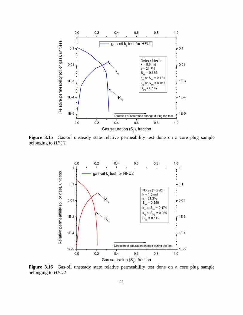
Figure 3.152Gas-oil unsteady state relative permeability test done on a core plug sample
belonging to HFU1 ....................................................................................................... 41
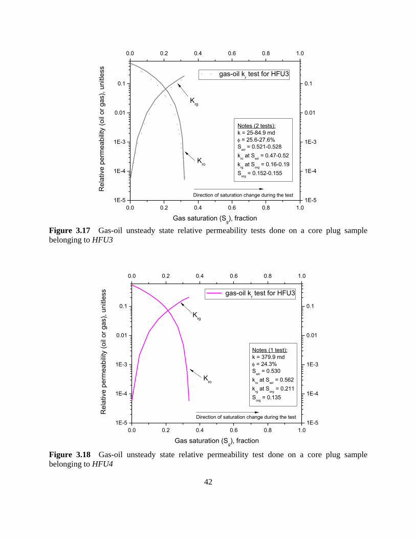
Figure 3.162Gas-oil unsteady state relative permeability test done on a core plug sample
belonging to HFU2 ....................................................................................................... 41
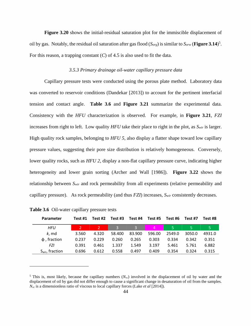
Figure 3.172Gas-oil unsteady state relative permeability tests done on a core plug sample
belonging to HFU3 ....................................................................................................... 42
Figure 3.182Gas-oil unsteady state relative permeability test done on a core plug sample
belonging to HFU4 ....................................................................................................... 42
Figure 3.192Gas-oil unsteady state relative permeability tests done on a core plug sample
belonging to HFU5 ....................................................................................................... 43
Figure 3.202Experimental initial-residual saturation plot for immiscible displacement of oil
by gas ............................................................................................................................ 43
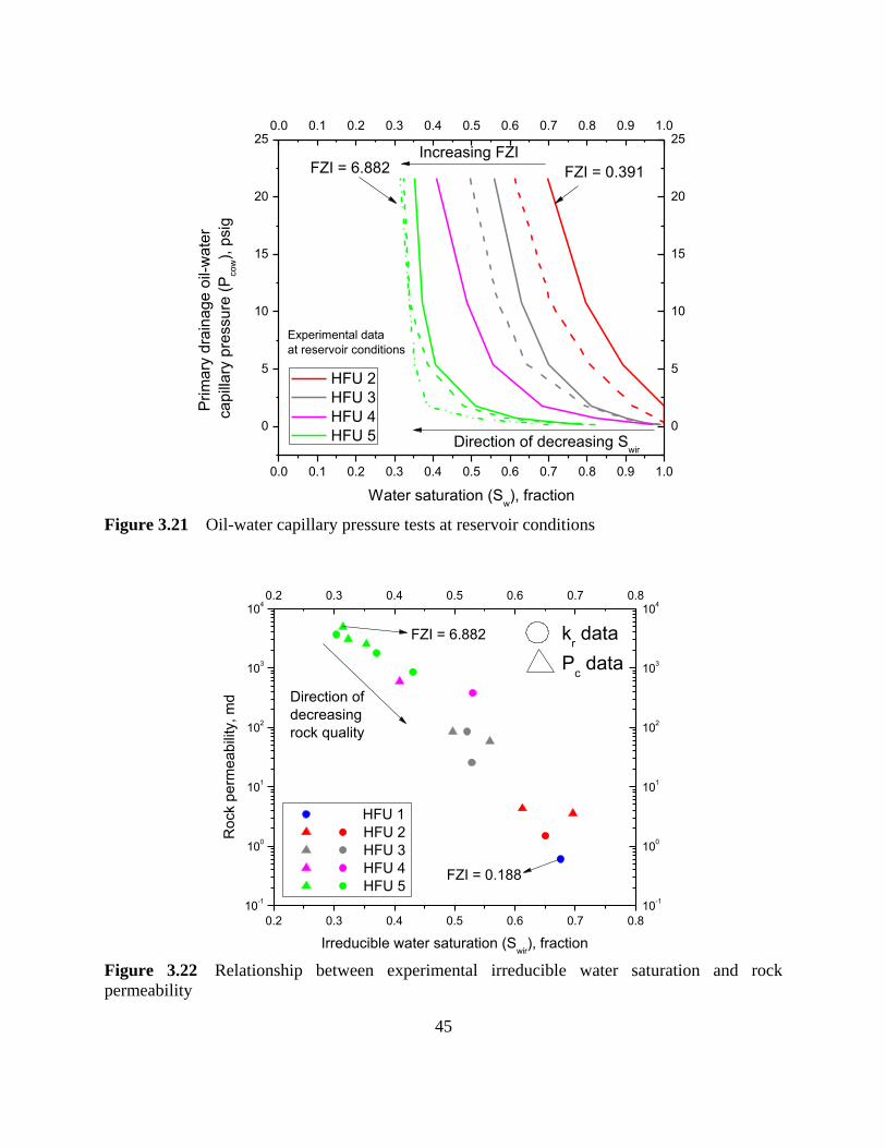
Figure 3.213Oil-water capillary pressure tests at reservoir conditions ........................................ 45
Figure 3.223Relationship between experimental irreducible water saturation and rock
permeability .................................................................................................................. 45
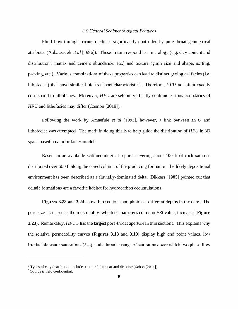
Figure 3.233Thin sections for three of the five hydraulic from units: HFU2 (a), HFU3 (b)
and HFU5 (c) (figures a, b and c printed with permission from Zeus OL Peru SAC
[2016]) .......................................................................................................................... 47
Figure 3.243Core photos showing variations in rock texture (figures a through e printed
with permission from Zeus OL Peru SAC [2016]) ...................................................... 48
Page 13
xiii
LIST OF TABLES
Page
Table 1.1 Reservoir and fluid properties........................................................................................ 4
Table 2.12Analog PVT data .......................................................................................................... 9
Table 2.22Average absolute relative error between fluid property correlations in McCain et
al [2011] and experimental PVT data ........................................................................... 15
Table 3.14Average FZI values for each HFU ............................................................................. 33
Table 3.24Unsteady state water-oil relative permeability tests ................................................... 36
Table 3.34Displacement efficiency at residual oil saturation after waterflood from unsteady
state water-oil relative permeability tests ..................................................................... 36
Table 3.44Unsteady state gas-oil relative permeability tests ....................................................... 40
Table 3.54Displacement efficiency at residual oil saturation after gas flood from unsteady
state gas-oil relative permeability tests ........................................................................ 40
Table 3.64Oil-water capillary pressure tests ................................................................................ 44
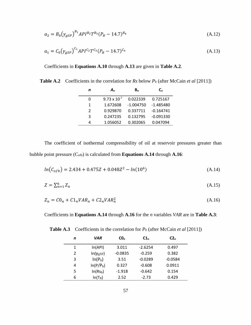
Table A.14Coefficients in the correlation for Pb (after McCain et al [2011]) ............................. 56
Table A.24Coefficients in the correlation for Rs below Pb (after McCain et al [2011]) ............. 57
Table A.34Coefficients in the correlation for Pb (after McCain et al [2011]) ............................. 57
Page 14
1
CHAPTER I
INTRODUCTION
1.1 Statement of the Problem
Production from an oil field located in northern Perú started in 2007. Within 6 years of
production, the reservoir pressure dropped to almost 10% its initial value, resulting in a steep
production decline. In 2015, a waterflooding pilot project was started. Although initial results
were promising, the subsequent field wide implementation of the project has not met the operator’s
expectations. Injected water breakthrough has occurred earlier than expected and incremental oil
is less than the anticipated volume. A reservoir (rock and fluid) characterization was done to better
understand the displacement process. Leading industry-proven techniques were applied.
1.2 Research Outline
Rock and fluid characterization of a Peruvian oil field is presented in Chapter II and
Chapter III.
Chapter II presents the reservoir fluid characterization. The primary objective of this
chapter is to introduce representative pressure-volume-temperature (PVT) relationships and
relevant associated fluid properties. Lack of actual PVT samples taken at early stages of field
development made impossible to establish such relationship in the laboratory. Thus, well logs,
production and pressure data, analog PVT samples and fluid property correlations were used.
Chapter III depicts the reservoir rock characterization. The primary objective of this
chapter is to describe the reservoir rock in terms of hydraulic flow units (HFU). Such
representation was done by means of the flow zone indicator (FZI) and rock quality index (RQI)
Page 15
2
parameters. This approach, originally proposed by Amaefule et al [1993], was combined with
hierarchical cluster analysis to objectively determine the optimum number of HFU and their
corresponding FZI values in a way similar to that presented by Abbaszadeh et al [1996] and
Dezfoolian et al [2013]. The approach proposed in this thesis differs from the latest in at least two
ways. First, the absolute error measurement of each cluster is replaced by a relative error
measurement. Secondly, the similarity measurement is defined as the L1 norm (i.e. city block or
Manhattan distance).
1.3 Field Case Description
All methods and analysis presented here were applied to an oil field located in northern
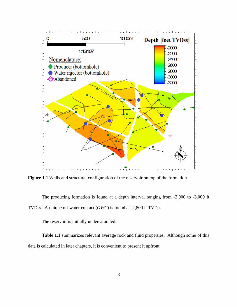
Perú. Main producing formation is locally named Salinas (Eocene). Figure 1.1 shows a structural
map on top of the formation along with the bottomhole position of the wells. There are 40 wells
in total. Production started in 2007 and within 6 years the reservoir pressure had dropped to almost
10% its initial value. The severe pressure depletion resulted in a steep production decline.
In 2015, a waterflooding pilot project was started, and by 2018 there were 7 water injectors.
Repressurization by water injection from reservoir pressures lower than the bubble point pressure
(Pb) would have resulted in a collapsing gas saturation, and implies a situation of repressurization
under variable bubble point pressure.
Page 16
3
Figure 1.1 Wells and structural configuration of the reservoir on top of the formation
The producing formation is found at a depth interval ranging from -2,000 to -3,000 ft
TVDss. A unique oil-water contact (OWC) is found at -2,800 ft TVDss.
The reservoir is initially undersaturated.
Table 1.1 summarizes relevant average rock and fluid properties. Although some of this
data is calculated in later chapters, it is convenient to present it upfront.
Page 17
4
Table 1.1 Reservoir and fluid properties
Reservoir Properties:
Gross thickness, h = 1,000 ft
Estimated net to gross ratio, NTG = 0.53
Average porosity, ϕ = 0.109 (fraction)
Average irreducible water saturation, Swirr = 0.767 (fraction)
Average permeability, k = 8.9 md
Average depth to reservoir top = -2,000 ft TVDss
Average depth to reservoir base = -3,000 ft TVDss
Original oil-water contact, OWC = -2,800 ft TVDss
Fluid Properties:
API gravity, °API = 42
Bubble point pressure, Pb = 1,526 psia
Oil formation volume factor at Pi, Boi = 1.1496 RB/STB
Oil viscosity at Pi, oi = 1.5426 cp
Solution gas-oil ratio at Pi, Rsi = 326 SCF/STB
Oil compressibility at Pi, coi = 9.17x10⁻⁶ psi-1
Additional Information:
Initial reservoir pressure, Pi = 1,785 psia
Datum depth = -2,500 ft TVDss
Original gas cap to oil reservoir volume ratio, m = 0 RB/RB
Page 18
5
CHAPTER II
RESERVOIR FLUID CHARACTERIZATION
The main challenge for the characterization of the reservoir fluid was the lack of PVT
laboratory analysis. Uncertainty therefore existed for all fundamental fluid properties such as
bubble point pressure (Pb), solution gas-oil ratio at the bubble point (RSB), etc. Other sources of
information had to be evaluated. These included well log data, production history, analog fluid
PVT reports and fluid property correlations.
2.1 Literature Review
If laboratory PVT data are not available, published correlations are frequently used for
estimation of reservoir fluid properties as a function of pressure. Many correlations have been
published for gas, oil and water. McCain et al [2011] however, compiled this vast number of
correlations and systematically determine their accuracy by comparing their predicted properties
with a large set of measured fluid property data. Measured data covered the full range of conditions
and properties that might be found in practice. For these correlations to yield a representative
description of the reservoir fluid, accurate input parameters, such as bubble point pressure (Pb) and
solution gas-oil ratio at the bubble point (RSB) among others, need to be provided.
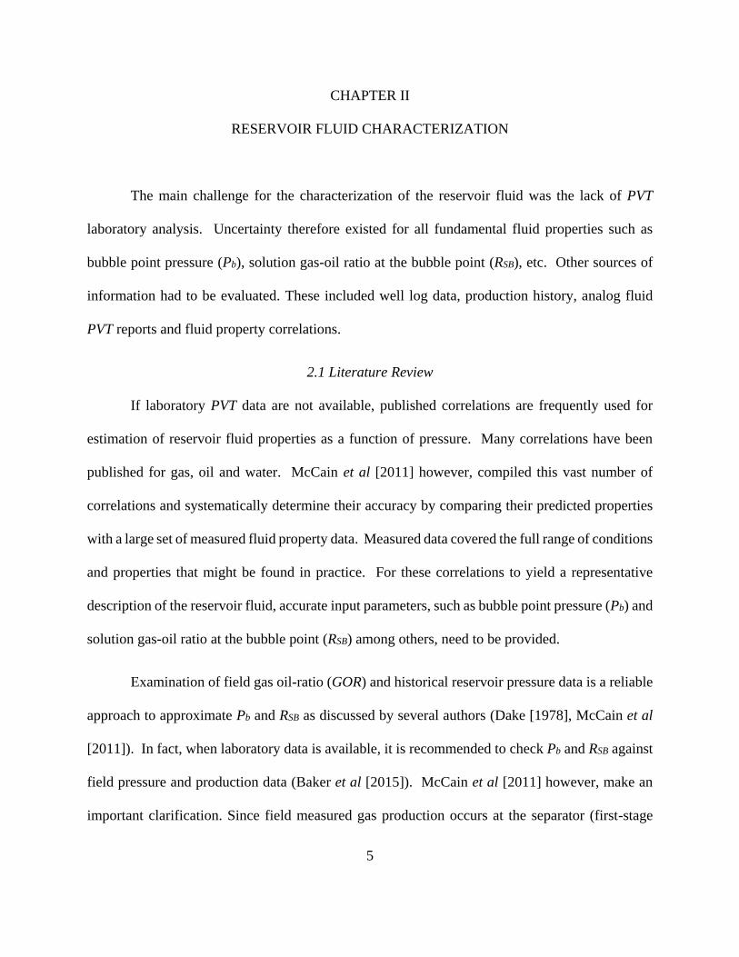
Examination of field gas oil-ratio (GOR) and historical reservoir pressure data is a reliable
approach to approximate Pb and RSB as discussed by several authors (Dake [1978], McCain et al
[2011]). In fact, when laboratory data is available, it is recommended to check Pb and RSB against
field pressure and production data (Baker et al [2015]). McCain et al [2011] however, make an
important clarification. Since field measured gas production occurs at the separator (first-stage
Page 19
6
separator usually), then estimates of the gas volume vented from the stock tank must be made and
added in order to obtain true values of the solution gas-oil ratio at the bubble point pressure (RSB).
Well log data can also be helpful in estimating Pb. In particular, Neutron-Density logs are
used in the practice to establish the position of the gas-oil contact (GOC). If these logs are run
early in the life of a reservoir having an original gas cap, the depth to the original GOC can be
established. The reservoir pressure corresponding at that depth would equal Pb (Baker et al
[2015]). For an undersaturated oil reservoir, no gas cap would exist at initial conditions and the
Neutron-Density logs would not have a crossover. In this case, no direct estimate of Pb can be
made, but an upper limit can be defined as Pb must not be greater than the initial reservoir pressure
(measured at any height in the oil column).
Analog PVT data is another option if no laboratory analysis were conducted on fluid
samples from the actual reservoir. As in the case of any oil PVT analysis, representative fluid
samples could only be obtained if the reservoir pressure, and the pressure at the bottom of the test
well at the time of sampling, do not drop below Pb (Archer et al [1986], McCain [1990]). Samples
can be obtained either at the surface or downhole. In general, a sample is valid if the gas and liquid
are in equilibrium at the time of sampling (Pedersen et al [2015] and McCain [2016]).
Not only fluid samples need to be valid for a PVT study to be representative. The lab work
itself has to be accurate as well. McCain [2016] has proposed a workflow to validate the accuracy
of laboratory analysis. He suggests using reliable fluid property correlations, such as those in
McCain et al [2011], to check the accuracy of laboratory data.
Page 20
7
2.2 Field Gas Oil-Ratio
Figure 2.1 shows the historical producing gas-oil ratio from the separator, i.e. RSP or field
GOR data, and reservoir pressure data. As of early 2008, RSP starts increasing, marking the point
in time at which the reservoir pressure drops below Pb. From this data, limiting values of Pb and
RSP were defined as follows: 1,400 psia < Pb < 1,785 psia; and 200 SCF/STB < RSP < 600 SCF/STB.
Early drill stem test (DST) in the field helped defined RSP as 326 SCF/STB.
Figure 2.12Field GOR and reservoir pressure (Pr) history
Two observation are worth making. First, early RSP data in Figure 2.1 differs from RSB by
the amount of gas produced at the stock tank. The producing gas-oil ratio from the stock-tank
(RST) must be added to RSP data if a more precise estimation of RSB is needed. Since in practice
RST is seldom measured, McCain et al [2011] recommends to increase RSP by 16.2%. A second
observation is that the decrease in RSP in 2011 is not due to water injection, which started in 2015.
2006 2008 2010 2012 2014 2016
0
1000
2000
3000
40002006 2008 2010 2012 2014 2016
GOR (SCF/STB)
Pr (psia)
Time, year
Fie
ld G
OR
, S
CF
/ST
B
Pi = 1,785 psia
From DST:
RSP
=326SCF/STB
Pr < P
b
Start of waterflood
0
200
400
600
800
1000
1200
1400
1600
1800
2000
Me
asu
red
rese
rvo
ir pre
ssu
re, p
sia
Page 21
8
This decline is due to the behavior of the gas formation volume factor (Bg) at low pressures, causing
Bg to increase more rapidly than the increasing gas relative mobility (Slider [1983]).
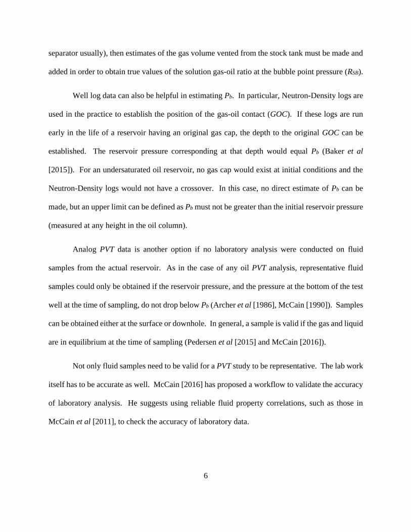
2.3 Well Log Data
Well log data also confirmed the reservoir was originally subsaturated and help
constraining Pb. Figure 2.2 shows well logs data in 5 wells located high in the reservoir structure.
Of particular interest is Well 3, which was drilled early in the life of the reservoir and showed no
indications of an original gas cap. Additionally, during drill stem test (DST) operations the well
flowed oil and gas from perforations at the top of the producing formation.
Figure 2.23Well log data in structurally high wells
Top of producing formation
OWC -2800 ft TVDss
Dec-2009 → Logging datesOct-2011 May-2015 Aug-2010Jul-2008
Intervals tested close to the top of the structure yielded oil with some gas. There is no evidence of initial gas cap.
1
2
3
1
2
Notes
3
Well 1 Well 2 Well 3 Well 4 Well 5
Flow test: oil and gas
Gamma Ray log
Neutron-Density crossover (suggestive of free gas)
Page 22
9
The absence of a gas cap at original conditions meant Pb was lower than the reservoir
pressure at the top of the structure.
2.4 Analog PVT Data
Three PVT studies (i.e. laboratory analysis) done on samples collected from nearby analog
reservoirs were available. Table 2.1 summarizes some relevant data.
Table 2.12Analog PVT data
Sample number
Sample location
°API Pb
(psia) Temperature
(°F) RSB
(SCF/STB)
1 Separator 35.4 122 122 283
2 Downhole 43.6 119 119 357
3 Downhole 39.5 118 118 389
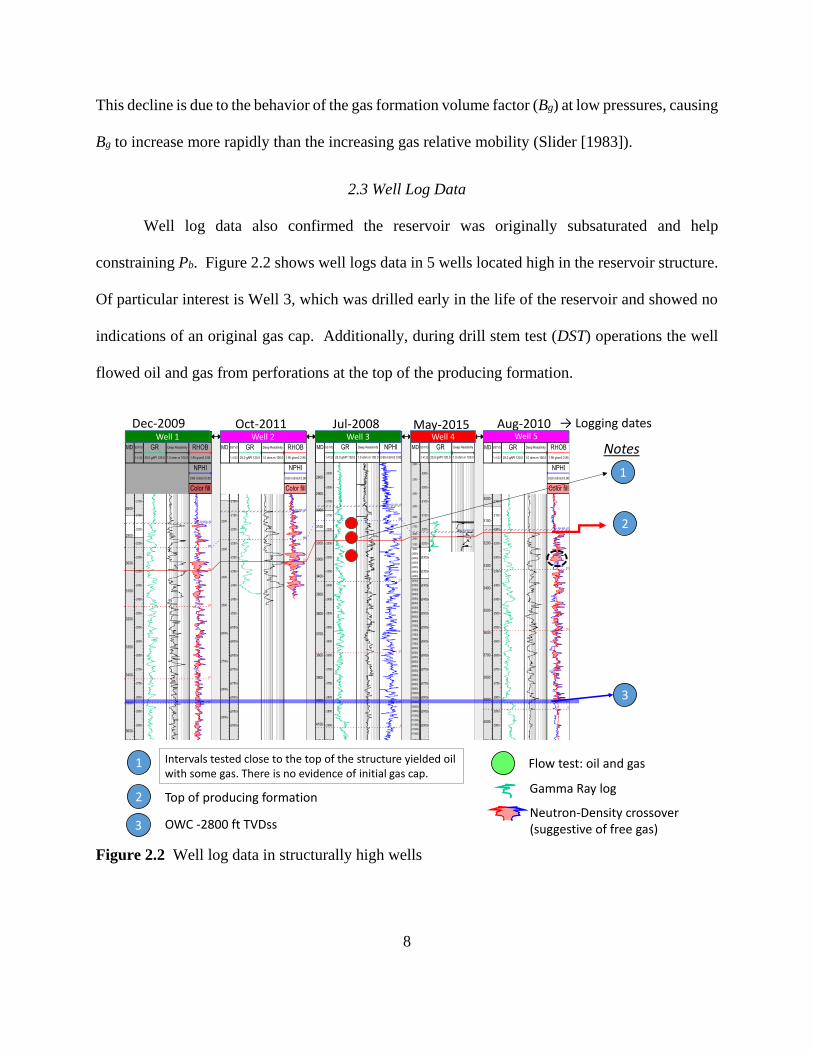
Validation of analog PVT information was done in two steps: first, vapor-liquid equilibrium
(VLE) at the time of sampling was checked to determine the validity of the samples; and secondly,
the lab work itself was validated through the method proposed by McCain [2016]. The workflow
is presented in detail in Figure 2.3. Validation of fluid samples can only be attempted for surface
(i.e. separator) samples though, and no method exists in the industry to validate downhole samples
(McCain [2016]).
Additional details on the workflow depicted in Figure 2.3 are presented in the next two
sections.
Page 23
10
Figure 2.34Workflow proposed by McCain [2016] for validation of fluid samples and PVT
laboratory analysis
2.4.1 Validation of fluid samples
For surface (i.e. separator) fluid samples to be valid for further PVT laboratory analysis,
the sampled separator gas and separator liquid must be in equilibrium (McCain et al [2016] and
Pedersen et al [2015]). At equilibrium conditions, the separator gas is at its dew point and the
separator oil at its bubble point. This means that the phase envelopes of the separator gas and
separator liquid have a point of intersection at the separator conditions (Pedersen et al [2015]).
Figure 2.4 illustrates this point.
Input data: PVT lab study
End Experimental k= theoretical k ?
Yes
Calculate experimental equilibrium ratios (k-factors)
Surface samples?
No
Obtain theoretical equilibrium ratios and compare with experimental k
Yes
Samples are valid
Start lab work validation?
Downhole samples cannot be validated. Be cautious
No
Yes
Perform “smell test”
Calculate all fluid properties (ρ, μ, etc.) using McCain et al [2011] correlations
Lab properties agree?
No
Yes
Lab work is invalid Lab work is valid
End End
Page 24
11
Figure 2.45Phase envelopes of a separator gas and separator oil (after Pedersen et al [2015])
A reasonably accurate way to predict vapor-liquid equilibrium (VLE) is through
correlations based on experimental observations of VLE behavior (McCain [1990]). These
correlations, such as Bruno et al [1972], invoke use of equilibrium ratios, or k-factors, for the
different components in a mixture. For a component j, its k-factor is defined as follows:
𝑘𝑗 = 𝑦𝑗
𝑥𝑗 (2.1)
Where yj and xj are the gas and liquid compositions respectively that exist at equilibrium at
a given pressure and temperature. These compositions are given as mole fractions, and are
experimentally determined.
Theoretically derived k-factors, using the correlation by Bruno et al [1972], were compared
against experimental k-factors to assess the quality of fluid samples. Agreement between the two
would exist if the sampled gas and liquid are in equilibrium (Pedersen et at [2015] and McCain
[2016]). Pressure and temperature conditions are those prevailing at the separator for surface fluid
samples. Figure 2.5 is such a plot for the analog surface fluid sample. In this plot, k-factors
Page 25
12
correspond to a pressure and temperature of 45 psig and 90 °F, which were the reported sampling
conditions. In this plot, the abscissa is the Hoffman, Crump & Hocott (HCH) plotting function
defined by Hoffman et al [1953] as:
𝐻𝐶𝐻 = [log(𝑃𝐶𝑗)−log(14.7)
1
𝑇𝐵𝑗−
1
𝑇𝐶𝑗
] [1
𝑇𝐵𝑗−
1
𝑇] (2.2)
Where PCj and TCj are the critical pressure and critical temperature, TBj is the normal boiling
point and T is the prevailing temperature. All pressures and temperatures are in absolute quantities.
The linear trend of the experimental k-factors in Figure 2.5 suggested the sampled gas and
liquid were in equilibrium. However, the disagreement with the theoretical k-factors implied the
samples were in equilibrium at conditions other than those reported.
Figure 2.56Experimental and theoretical k-factors against the Hoffman, Crump & Hocott plotting
function at reported separator pressure and temperature: assessment of equilibrium for analog oil
and gas surface samples
0.0 0.5 1.0 1.5 2.0 2.5
10-1
100
101
0.0 0.5 1.0 1.5 2.0 2.5
10-1
100
101
nC5
iC5
nC4
iC4
C3
C1
Experimental
Theoretical
k-f
acto
rs
(dim
ensio
nle
ss)
HCH plotting function (dimensionless)
Bruno-Yanosik correlation
Equilibrium K-factors for a surface fluid sample
Pure components C1 to C
5
C2
Laboratory reported sampling conditions
P = 45 psig; T = 90 °F
Page 26
13
The theoretical k-factors were recalculated at a separator pressure and temperature of 45
psig and 110 °F. Figure 2.6 plots the data. Agreement between experimental and theoretical k-
factors suggests these were the likely actual equilibrium conditions.
Figure 2.67Experimental and theoretical k-factors against the Hoffman, Crump & Hocott plotting
function at likely actual separator pressure and temperature: assessment of equilibrium for analog
oil and gas surface samples
In Figures 2.5 and 2.6 the only components shown are C1 thorough n-C5 because the
compositional analysis did not discriminate higher molecular weight isomers.
Based on the previous analysis, the analog surface fluid sample was considered valid. On
the other hand, the validity of the downhole samples remained unknown, as this analysis is not
applicable.
The next stage in the workflow (Figure 2.3) was to validate the laboratory work itself.
0.0 0.5 1.0 1.5 2.0 2.5
10-1
100
101
0.0 0.5 1.0 1.5 2.0 2.5
10-1
100
101
nC5
iC5
nC4
iC4
C3
C1
Experimental
Theoretical
k-f
acto
rs
(dim
ensio
nle
ss)
HCH plotting function (dimensionless)
Bruno-Yanosik correlation
Equilibrium K-factors for a surface fluid sample
Pure components C1 to C
5
C2
Likely actual sampling conditions
P = 45 psig; T = 110 °F
Page 27
14
2.4.2 Validation of laboratory work
This section includes a direct field application of a robust workflow to validate laboratory
work proposed by Professor William D. McCain, Jr. at Texas A&M University (McCain [2016]).
He proposes a two-step approach. First, an overall quality check of the laboratory report is done,
and visible inconsistencies are determined by a limited number of calculations. This step was
named “smell test”. Secondly, reliable fluid property correlations, such as those in McCain et al
[2011], are used to check the accuracy of laboratory data.
A quality check done during the “smell test” involves use of the following equation:
𝐵𝑜𝑏 =𝜌𝑜+0.01357𝑅𝑆𝐵𝛾𝑔
𝜌𝑜𝑅𝑏 (2.3)
Where Bob and ρob are the oil formation volume factor and oil density at the bubble point
in RB/STB and lb/ft3 respectively, and γg is the weighted average gas specific gravity. Equation
2.3 is not a correlation, but the result of a material balance (McCain et al [2011]).
In short, the “smell test” was perform on all three samples and no inconsistencies were
found. For example, application of Equation 2.3 to the data from differential liberation tests and
separator tests revealed a difference of about 2% in most cases.
Next, relevant fluid properties were calculated using the correlations by McCain et al
[2011]. They are reproduced from McCain et al [2011] in Appendix A. Input parameters for these
correlations were laboratory RST and RSP from the separator test; API gravity; laboratory separator
gas and stock-tank gas specific gravities (γgSP and γgST); and temperature of the laboratory PVT
cell.
Page 28
15
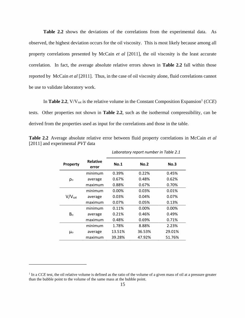
Table 2.2 shows the deviations of the correlations from the experimental data. As
observed, the highest deviation occurs for the oil viscosity. This is most likely because among all
property correlations presented by McCain et al [2011], the oil viscosity is the least accurate
correlation. In fact, the average absolute relative errors shown in Table 2.2 fall within those
reported by McCain et al [2011]. Thus, in the case of oil viscosity alone, fluid correlations cannot
be use to validate laboratory work.
In Table 2.2, V/Vsat is the relative volume in the Constant Composition Expansion1 (CCE)
tests. Other properties not shown in Table 2.2, such as the isothermal compressibility, can be
derived from the properties used as input for the correlations and those in the table.
Table 2.23Average absolute relative error between fluid property correlations in McCain et al
[2011] and experimental PVT data
Laboratory report number in Table 2.1
Property Relative
error No.1 No.2 No.3
minimum 0.39% 0.22% 0.45%
ρo average 0.67% 0.48% 0.62%
maximum 0.88% 0.67% 0.70%
minimum 0.00% 0.03% 0.01%
V/Vsat average 0.03% 0.04% 0.07%
maximum 0.07% 0.05% 0.13%
minimum 0.11% 0.00% 0.00%
Bo average 0.21% 0.46% 0.49%
maximum 0.48% 0.69% 0.71%
minimum 1.78% 8.88% 2.23%
μo average 13.51% 36.53% 29.01%
maximum 39.28% 47.92% 51.76%
1 In a CCE test, the oil relative volume is defined as the ratio of the volume of a given mass of oil at a pressure greater
than the bubble point to the volume of the same mass at the bubble point.
Page 29
16
The error metric presented in Table 2.2 is the average absolute relative error (AARE). For
n measurements at n different pressures of an experimental variable (yexp), the average deviation
of a correlated variable ycor is defined as:
𝐴𝐴𝑅𝐸 =100
𝑛∑ |
𝑦𝑐𝑜𝑟−𝑦𝑒𝑥𝑝
𝑦𝑒𝑥𝑝|𝑛
𝑖=1 (2.4)
Equation 2.4 is the same error metric used by McCain et al [2011].
Given the small AARE values in Table 2.2, and following the proposed approach by
Professor William D. McCain, Jr., the analog PVT laboratory work was considered valid.
2.5 Reservoir Fluid Model
Validated analog PVT data and fluid property correlations were combined together to yield
a description of the reservoir fluid that suits the actual reservoir temperature, API gravity and
estimated RSB from production data (Table 1.1). Specifically, correlations by McCain et al [2011]
were used to estimate all gas and oil properties. These correlations are reproduced in Appendix
A. In the case of oil viscosity however, analog PVT data was used alone, as it is more
representative of this reservoir fluid than fluid correlations. Input parameters for these
correlations, such as solution gas-oil ratio at the bubble point (RSB), were estimated from
production data and field measurements.
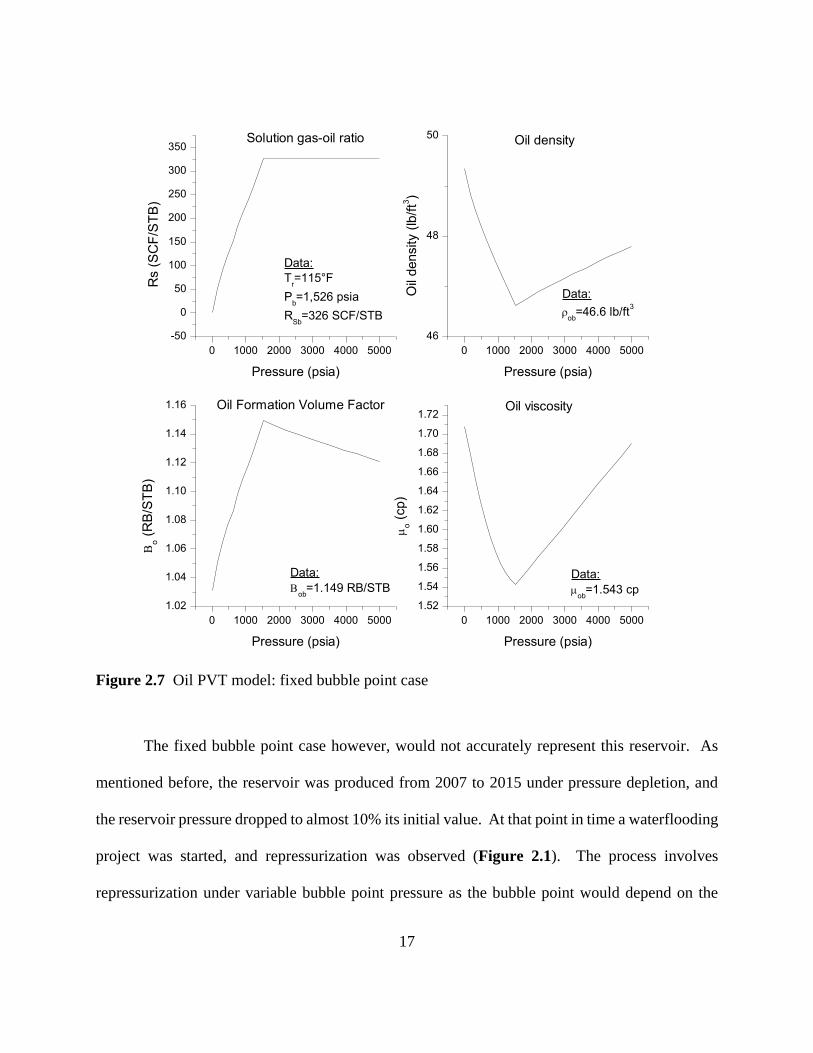
Figure 2.7 presents the resulting oil PVT data. Data depicted in this figure corresponds to
a fixed bubble point pressure case. The fluid model is black-oil, meaning all changes in the system
are determined mainly as a function of pressure (Wattenbarger [2000]). In Figure 2.7 all
properties are given at a fixed reservoir temperature of 115 °F.
Page 30
17
Figure 2.78Oil PVT model: fixed bubble point case
The fixed bubble point case however, would not accurately represent this reservoir. As
mentioned before, the reservoir was produced from 2007 to 2015 under pressure depletion, and
the reservoir pressure dropped to almost 10% its initial value. At that point in time a waterflooding
project was started, and repressurization was observed (Figure 2.1). The process involves
repressurization under variable bubble point pressure as the bubble point would depend on the
0 1000 2000 3000 4000 5000
-50
0
50
100
150
200
250
300
350
Data:
ob
=1.543 cp
Solution gas-oil ratioR
s (
SC
F/S
TB
)
Pressure (psia)
Data:
Tr=115°F
Pb=1,526 psia
RSb
=326 SCF/STB
0 1000 2000 3000 4000 5000
46
48
50
Data:
ob
=46.6 lb/ft3
Oil density
Oil
density (
lb/f
t3)
Pressure (psia)
0 1000 2000 3000 4000 5000
1.02
1.04
1.06
1.08
1.10
1.12
1.14
1.16
Data:
ob
=1.149 RB/STB
Oil Formation Volume Factor
o (
RB
/ST
B)
Pressure (psia)
0 1000 2000 3000 4000 5000
1.52
1.54
1.56
1.58
1.60
1.62
1.64
1.66
1.68
1.70
1.72Oil viscosity
o (
cp)
Pressure (psia)
Page 31
18
available gas. In fact, waterfloods applied to saturated oil reservoirs frequently cause the gas
saturation in regions near the injectors to reduce to zero at pressures below the original bubble
point (Wattenbarger [2000]).
Figure 2.8 presents the variable bubble point oil PVT model. Each line in this figure
represents undersaturated data with different solution gas-oil ratios, and thus different bubble
points. As shown in Figure 2.8, data has been extrapolated above the original bubble point
pressure. This is required for an accurate representation of repressurization processes with variable
bubble point (McCain and Spivey [1999] and Wattenbarger [2000]). Consistencies of oil and gas
properties were checked by ensuring that the oil compressibility (co) remains positive throughout
the range of extrapolated pressure. The formal definition of co is given by Equation 2.5.
𝑐𝑜 = −1
𝐵𝑜[(
𝜕𝐵𝑜
𝜕𝑃)
𝑇− 𝐵𝑔 (
𝜕𝑅𝑠
𝜕𝑃)
𝑇] (2.5)
Thus, for co to remain positive and pass the compressibility check, the following inequality
must be satisfied (McCain and Spivey [1999]):
∆𝐵𝑜 < 𝐵𝑔∆𝑅𝑠 (2.6)
In Equation 2.6, the value of the gas formation volume factor (Bg) is determined at the
lower pressure.
Additionally, in Figure 2.8 the maximum pressure along the abscissa has also been
increased to ensure that at all times and for all gridblocks, the simulator will interpolate, rather
than extrapolate, the PVT data.
Page 32
19
Figure 2.89Oil PVT model: variable bubble point case. Green lines reproduce the oil properties
previously shown in the fixed bubble point case
0 2000 4000 6000 8000 10000
300
600
900
1200
1500
300
600
900
1200
1500
0 2000 4000 6000 8000 10000
1.00
1.05
1.10
1.15
1.20
1.25
1.30
1.35
1.00
1.05
1.10
1.15
1.20
1.25
1.30
1.35
0 2000 4000 6000 8000 10000
1.4
1.5
1.6
1.7
1.8
1.9
2.0
2.1
1.4
1.5
1.6
1.7
1.8
1.9
2.0
2.1
Rs (
SC
F/S
TB
)
Pressure (psia)
o (
RB
/ST
B)
Pressure (psia)
52.7 239.7 326.0 422.9 621.2
819.5 1017.9 1216.2 1414.5 1612.9
o (
cp
)
Pressure (psia)
Solution gas-oil ratios (SCF/STB):
Page 33
20
2.6 Summary
Lack of PVT data from actual fluid samples was overcome by means of analog PVT data
and reliable fluid property correlations. Input parameters for these correlations, such as solution
gas-oil ratio at the bubble point (RSB), were estimated from production data and field
measurements. Analog PVT data was validated beforehand by comparison of experimental and
theoretical equilibrium ratios, or k-factors, and through the application of a robust workflow
originally proposed by Professor William D. McCain, Jr. at Texas A&M University (McCain
[2016]).
The resulting fluid model is a black-oil variable bubble point model, in which internal
consistencies of gas and oil properties were checked by ensuring that the oil compressibility (co)
remains positive throughout the range of extrapolated pressure.
Page 34
21
CHAPTER III
RESERVOIR ROCK CHARACTERIZATION
Characterization of the reservoir rock is required for proper representation of rock
properties in a tridimensional model. The underlying challenge is to identify relationships between
the observed rock properties in core samples, and then use those relationships to predict
permeability, and other rock properties, in uncored wells.
3.1 Literature Review
Estimation of permeability in uncored, but logged, wells has been a generic problem
common to all reservoirs. Therefore, procedures and methods have been sought to allow property
estimation at these locations. Traditional approaches include simple linear regressions between
core porosity and the logarithm of core permeability. Then, these regressions are applied to
uncored wells given some inference of porosity from log data.
More accurate predictions of permeability can be achieved by addressing the development
of permeability in porous rocks from fundamental concepts of geology and flow through porous
media (Abbaszadeh et al [1996]). Specifically, the intent is to define functional relationships for
permeability based on pore-throat geometry parameters. This is best achieved by identifying and
grouping portions of rock within the reservoir having similar fluid conductivity. These groups are
known as hydraulic flow units (HFU).
Earlier definitions of HFU were provided by Bear [1972] and Ebanks [1987]. They defined
a HFU as a body of rock in which geological and petrophysical properties related to the flow of
fluids are consistent and predictably different from properties of other HFU.
Page 35
22
Several methods have been proposed in the literature for rock characterization based on
HFU. Stolz and Graves [2003] provides a summary of some of them. Notably, there is no
universally applicable method.
One of the most widely used methods was proposed by Amaefule et al [1993]. The method,
which is based on the Kozeny-Carman equation (Carman [1961]), defines a characteristic
parameter for each HFU named flow zone indicator (FZI). In the original work by Amaefule et al
[1993], FZI values were determined graphically, in which was later known as graphical clustering.
Graphical clustering of HFU is subjective, since the number of flow units, and their corresponding
limits, are not uniquely determined. A solution was later given by Abbaszadeh et al [1996]. They
proposed to use the Ward’ algorithm, an analytical technique in hierarchical cluster analysis, to
objectively evaluate HFU. Their work significantly advanced the method. However, the number
of cluster, i.e. HFU, in the Ward’s algorithm was an input, and therefore the evaluation still
suffered from subjectivity. Later on, other authors, such as Svirsky et al [2004] and Dezfoolian
et al [2013], adopted the elbow method2, a technique used in cluster analysis, to aid determining
the optimum number of HFU in a given data set.
3.2 The FZI Method
Amaefule et al [1993] introduced pore-throat parameters into their definition of HFU by
rearrangement of the Kozeny-Carman equation (Carman [1961]):
2 The elbow method is based on the observation that as the number of clusters increases, the sum of within-cluster
variance of each cluster is reduced. This is because having more clusters allows to capture finer groups of data objects
that are more similar to each other (Han et al [2012]).
Page 36
23
0.0314√𝑘
𝜙=
𝜙
1−𝜙
1
√𝐹𝑠𝜏 𝑆𝑔𝑣 (3.1)
Where Fs is the shape factor, a characteristic parameters of the porous media, τ is the
tortuosity, and Sgv is the surface area per unit grain volume. The product Fsτ2 is known as the
Kozeny constant, and usually varies between 5 and 100 for most reservoir rocks (Abbaszadeh et
al [1996]). The constant 0.0314 is the conversion factor from μm2 to md.
Amaefule et al [1993] defined the flow zone indicator (FZI), rock quality index (RQI) and
void ratio (ϕz) as in Equations 3.2 through 3.4.
𝑅𝑄𝐼 = 0.0314√𝑘
𝜙 (3.2)
𝜙𝑧 =𝜙
1−𝜙 (3.3)
𝐹𝑍𝐼 =1
√𝐹𝑠𝜏 𝑆𝑔𝑣=
𝑅𝑄𝐼
𝜙𝑧 (3.4)
Rearrangement of Equation 3.1 with definitions in Equations 3.2 through 3.4 leads to a
linear form of the Kozeny-Carman equation after the logarithms are taken on both sides:
log(𝑅𝑄𝐼) = log(𝜙𝑧) + log(𝐹𝑍𝐼) (3.5)
Equation 3.5 suggests that rocks within a given HFU should exhibit a linear trend of unit
slope on a log-log plot of RQI against ϕz. Furthermore, estimation of the FZI for each HFU can
be graphically done by letting ϕz be 1. This is because at ϕz equal 1 the values of RQI and FZI are
the same. This approach is known as graphical clustering.
Page 37
24
In summary, data samples with similar FZI values will be close to a single unit-slope
straight line with a mean FZI value. Conversely, samples with significantly different FZI will lie
on other parallel unit-slope lines. Each line defines a HFU and has associated mean FZI value.
Permeability can be predicted for a given FZI and porosity values by rearrangement of
Equations 3.2 through 3.4.
𝑘 = 1014𝐹𝑍𝐼2 𝜙3
(1−𝜙)2 (3.5)
3.3 Hierarchical Cluster Analysis: an Overview
Objective definition of the number of HFU and their corresponding FZI values can be
achieved through hierarchical Cluster Analysis (Abbaszadeh et al [1996] and Dezfoolian et al
[2013]). This is a method in data mining and statistics in which a hierarchical decomposition of
the given data set is done. The method can be classified into agglomerative, if higher order clusters
are created, or divisive, if lower order groups are generated to break down starting higher order
groups of data objects (Han et al [2012]).
Of particular interest in HFU characterization is the agglomerative clustering. An
agglomerative hierarchical clustering method uses a bottom-up strategy. It typically starts by
letting each object form a cluster on its own, and then iteratively merges them into larger (higher
order) clusters, until all the objects in the data set are in a single cluster. The result is a tree-like
structure called the dendrogram (Figure 3.1).
Merging of clusters at each successive step is done in such a way that the similarity between
the objects within a given cluster is maximized. At the same time, the dissimilarity with the objects
of different clusters is maximized as well. Similarity, and therefore dissimilarity, is based on the
Page 38
25
distance between the two objects. Two objects are similar if they are close together. Because two
clusters are merged per iteration, where each cluster contains at least one object, an agglomerative
method requires at most as many iterations as the number of objects in the data set (Han et al
[2012]).
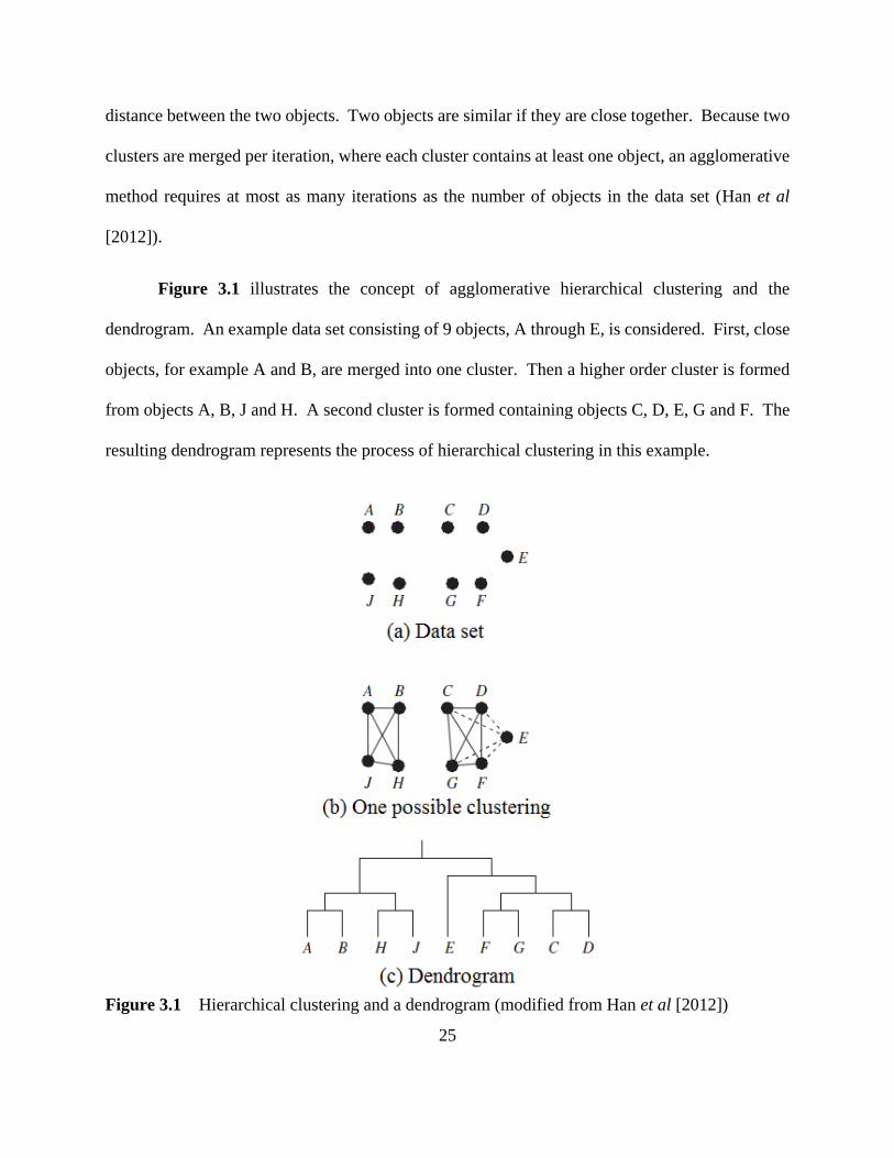
Figure 3.1 illustrates the concept of agglomerative hierarchical clustering and the
dendrogram. An example data set consisting of 9 objects, A through E, is considered. First, close
objects, for example A and B, are merged into one cluster. Then a higher order cluster is formed
from objects A, B, J and H. A second cluster is formed containing objects C, D, E, G and F. The
resulting dendrogram represents the process of hierarchical clustering in this example.
Figure 3.110Hierarchical clustering and a dendrogram (modified from Han et al [2012])
Page 39
26
Distance measures used for calculation of similarity, and therefore dissimilarity, between
numerical data points include the Euclidean (a.k.a. L2 norm) and Manhattan (a.k.a. L1 norm, or
City Block) distances. In general, these two are particular cases of a more general measure called
the Minkowski distance. The Minkowski distance is also known as the Lp norm. Given two
objects xi and xj defined in an l-dimensional space, the Minkowski distance is defined by Equation
3.6.
𝑑(𝑖, 𝑗) = √|𝑥𝑖1 − 𝑥𝑗1|𝑝
+ |𝑥𝑖2 − 𝑥𝑗2|𝑝
+ ⋯ + |𝑥𝑖𝑙 − 𝑥𝑗𝑙|𝑝𝑝
(3.6)
Where p is the order. For p=1, then Equation 3.6 reverts to the Manhattan or City Block
measure. For p=2, it reverts to the Euclidean distance.
3.4 Hydraulic Flow Units
More than 800 ft of core data, having about 340 measurements of porosity and permeability
were available. An early quality control revealed some plugs were reported damaged by the
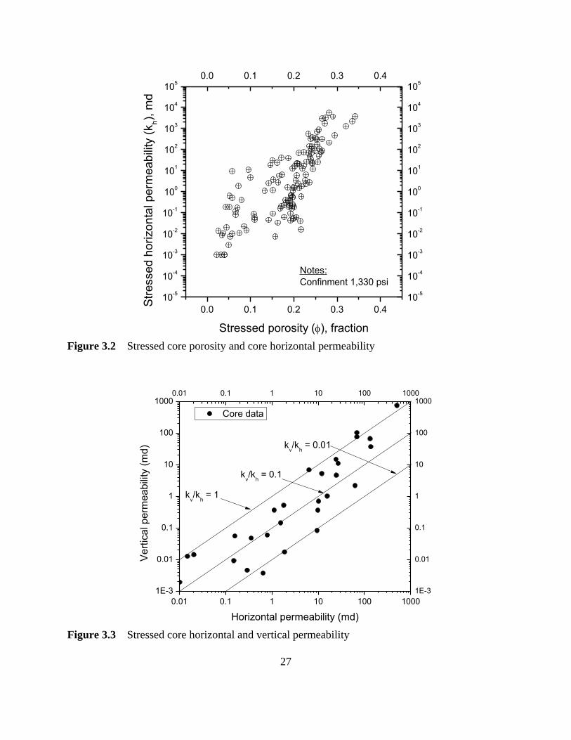
laboratory, and were dismissed from evaluation. Figure 3.2 shows valid core porosity and core
horizontal permeability data at an average confining stress of 1,330 psi3. Figure 3.2 presents core
vertical permeability data. For the purpose of defining hydraulic flow units (HFU) however, only
the data in Figure 3.2 is used.
Hierarchical cluster analysis was used instead of the traditional graphical clustering method
to objectively determine the number of HFU and their associated FZI values.
3 Amaefule et al [1993] recommended to use stressed porosity and permeability for evaluation of HFU.
Page 40
27
Figure 3.211Stressed core porosity and core horizontal permeability
Figure 3.312Stressed core horizontal and vertical permeability
0.0 0.1 0.2 0.3 0.4
10-5
10-4
10-3
10-2
10-1
100
101
102
103
104
105
0.0 0.1 0.2 0.3 0.4
10-5
10-4
10-3
10-2
10-1
100
101
102
103
104
105
Str
esse
d h
ori
zo
nta
l p
erm
ea
bili
ty (
kh),
md
Stressed porosity (), fraction
Notes:
Confinment 1,330 psi
0.01 0.1 1 10 100 1000
1E-3
0.01
0.1
1
10
100
10000.01 0.1 1 10 100 1000
1E-3
0.01
0.1
1
10
100
1000
kv/k
h = 0.01
kv/k
h = 0.1
Core data
Ve
rtic
al p
erm
eab
ility
(m
d)
Horizontal permeability (md)
kv/k
h = 1
Page 41
28
As discussed earlier, a fundamental need in cluster analysis is to measure the distance
between objects. When applied to the identification of HFU from core data, an intuitive choice
would be to measure distances in a plot of logarithm of RQI against logarithm of ϕz, as this is the
plot used for graphical clustering in the original work by Amaefule et al [1993]. Nonetheless, this
approach leads to a meaningless clustering as a single straight line in a log-log plot of RQI against
ϕz would intercept more than one cluster or flow unit (Figure 3.4).
Figure 3.413Example of an incorrect clustering of HFU
Meaningful clusters are obtained when distances are measured on the basis of the logarithm
of FZI as originally proposed by Abbaszadeh et al [1996]. This is because FZI values calculated
from actual field data usually exhibit a log-normal distribution resulting from the strong
dependency of FZI on permeability, which is often log-normally distributed.
Hierarchical cluster analysis was implemented in the form of a MATLAB code. The
algorithm is presented schematically in Figure 3.5. First, stressed core porosity and core
permeability data are provided as input. A quality control must be done before to ensure that the
input data are reliable. In this case, the laboratory report was inspected and rock samples reported
0.0 0.1 0.2 0.3 0.4
10-5
10-4
10-3
10-2
10-1
100
101
102
103
104
105
0.0 0.1 0.2 0.3 0.4
10-5
10-4
10-3
10-2
10-1
100
101
102
103
104
105
Str
esse
d h
ori
zo
nta
l p
erm
ea
bili
ty (
kh),
md
Stressed porosity (), fraction
Notes:
Confinment 1,330 psi
Cluster 1
Cluster 2
Cluster 3
Cluster 4
Cluster 5
0.01 0.1 1
10-3
10-2
10-1
100
1010.01 0.1 1
1E-3
0.01
0.1
1
10
RQ
I
Void Ratio or z (fraction)
Cluster 1
Cluster 2
Cluster 3
Cluster 4
Cluster 5
Page 42
29
as damaged were discarded. Next, Equations 3.2 to 3.4 are used to calculate FZI for each data
point. Similarity, and thus dissimilarity, measures are obtained on the basis of the logarithm of
FZI (Abbaszadeh et al [1996]). The dendrogram is then built by linkage of the dissimilarity
matrix4.
Figure 3.514Algorithm for hierarchical cluster analysis of hydraulic flow units
Objective definition of the number of HFU can be achieved by evaluation of the error in
FZI for a given number of clusters (Dezfoolian et al [2013]). The algorithm in Figure 3.5 starts
by assuming one cluster (i.e. one HFU). Then, an average FZI is obtained from the data set, and
an error metric is evaluated. The number of clusters is then increased, one at a time, up to a
4 The dissimilarity matrix is a symmetric matrix which stores the collection of distance measures for all pairs of n
objects, where n is the number of data points in the set.
Input data: k, φ
Calculate FZI and log(FZI)
Similarity measure log(FZI):Distances between data points
Initialize n = 0
Set n = n + 1
End
Linkage: build dendrogram
n = N?No
Yes
Stressed core porosity and permeability data
Choices: City Block (L1 norm), Euclidean distance (L2 norm)
Prune dendrogram to create n clusters
Calculate average FZI per cluster
Get average absolute relative error
Plot errors vs number of HFU:Select optimum n
N = maximum allowable number of flow units (e.g. 20)
xi = FZI for data point i in HFU n
Cn = average FZI of HFU n
n = number of clusters or hydraulic flow units (HFU)
Page 43
30
predefined maximum number (N). The average FZI values per cluster (i.e. per HFU) are
recalculated and the error metric in FZI is reevaluated each time. This process can be thought of
as pruning the dendrogram at different levels each time from its base to the top.
Averaging all FZI values within given clusters exactly corresponds to a linear least-squares
regression of the data (Abbaszadeh et al [1996]).
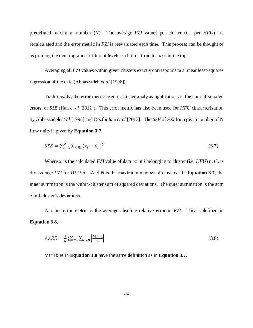
Traditionally, the error metric used in cluster analysis applications is the sum of squared
errors, or SSE (Han et al [2012]). This error metric has also been used for HFU characterization
by Abbaszadeh et al [1996] and Dezfoolian et al [2013]. The SSE of FZI for a given number of N
flow units is given by Equation 3.7.
𝑆𝑆𝐸 = ∑ ∑ (𝑥𝑖 − 𝐶𝑛)2𝑥𝑖∈𝑛
𝑁𝑛=1 (3.7)
Where xi is the calculated FZI value of data point i belonging to cluster (i.e. HFU) n. Cn is
the average FZI for HFU n. And N is the maximum number of clusters. In Equation 3.7, the
inner summation is the within-cluster sum of squared deviations. The outer summation is the sum
of all cluster’s deviations.
Another error metric is the average absolute relative error in FZI. This is defined in
Equation 3.8.
𝐴𝐴𝑅𝐸 =1
𝑁∑ ∑ |
𝑥𝑖−𝐶𝑛
𝐶𝑛|𝑥𝑖∈𝑛
𝑁𝑛=1 (3.8)
Variables in Equation 3.8 have the same definition as in Equation 3.7.
Page 44
31
Regardless of the error metric used, as the number of clusters, i.e. HFU, increases, the error
metric decreases. This is because the data set is being fit with an increasing number of functional
relationships (i.e. unit-slope straight lines in a plot of logarithm of RQI against logarithm of ϕz).
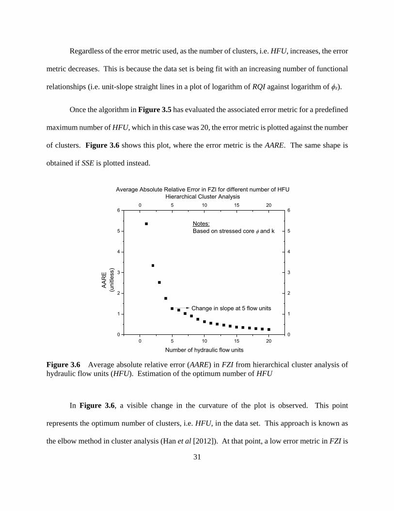
Once the algorithm in Figure 3.5 has evaluated the associated error metric for a predefined
maximum number of HFU, which in this case was 20, the error metric is plotted against the number
of clusters. Figure 3.6 shows this plot, where the error metric is the AARE. The same shape is
obtained if SSE is plotted instead.
Figure 3.615Average absolute relative error (AARE) in FZI from hierarchical cluster analysis of
hydraulic flow units (HFU). Estimation of the optimum number of HFU
In Figure 3.6, a visible change in the curvature of the plot is observed. This point
represents the optimum number of clusters, i.e. HFU, in the data set. This approach is known as
the elbow method in cluster analysis (Han et al [2012]). At that point, a low error metric in FZI is
0 5 10 15 20
0
1
2
3
4
5
60 5 10 15 20
0
1
2
3
4
5
6
AA
RE
(unitle
ss)
Number of hydraulic flow units
Average Absolute Relative Error in FZI for different number of HFU
Hierarchical Cluster Analysis
Notes:
Based on stressed core and k
Change in slope at 5 flow units
Page 45
32
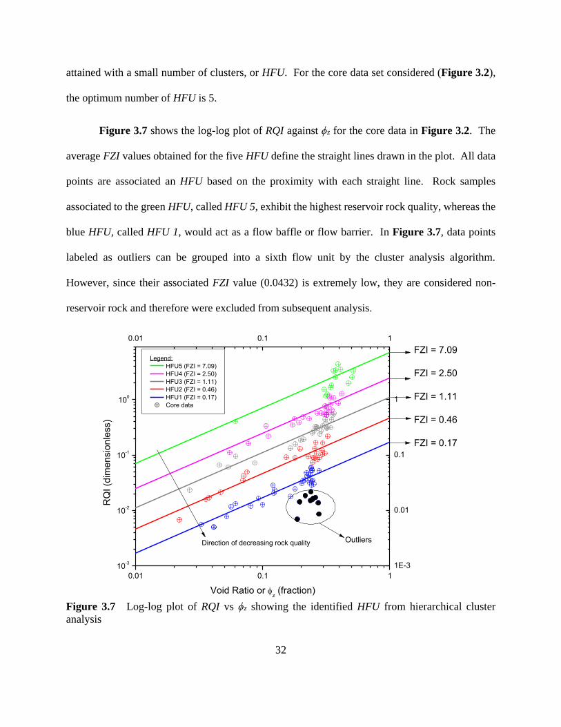
attained with a small number of clusters, or HFU. For the core data set considered (Figure 3.2),
the optimum number of HFU is 5.
Figure 3.7 shows the log-log plot of RQI against ϕz for the core data in Figure 3.2. The
average FZI values obtained for the five HFU define the straight lines drawn in the plot. All data
points are associated an HFU based on the proximity with each straight line. Rock samples
associated to the green HFU, called HFU 5, exhibit the highest reservoir rock quality, whereas the
blue HFU, called HFU 1, would act as a flow baffle or flow barrier. In Figure 3.7, data points
labeled as outliers can be grouped into a sixth flow unit by the cluster analysis algorithm.
However, since their associated FZI value (0.0432) is extremely low, they are considered non-
reservoir rock and therefore were excluded from subsequent analysis.
Figure 3.716Log-log plot of RQI vs ϕz showing the identified HFU from hierarchical cluster
analysis
0.01 0.1 1
10-3
10-2
10-1
100
0.01 0.1 1
1E-3
0.01
0.1
1
Legend:
HFU5 (FZI = 7.09)
HFU4 (FZI = 2.50)
HFU3 (FZI = 1.11)
HFU2 (FZI = 0.46)
HFU1 (FZI = 0.17)
Core data
Outliers
RQ
I (d
ime
nsio
nle
ss)
Void Ratio or z (fraction)
Direction of decreasing rock quality
FZI = 7.09
FZI = 2.50
FZI = 1.11
FZI = 0.46
FZI = 0.17
Page 46
33
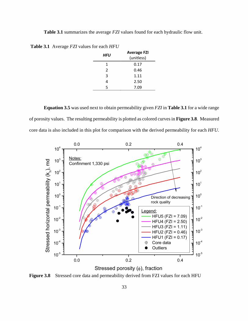
Table 3.1 summarizes the average FZI values found for each hydraulic flow unit.
Table 3.14Average FZI values for each HFU
HFU Average FZI
(unitless)
1 0.17
2 0.46
3 1.11
4 2.50
5 7.09
Equation 3.5 was used next to obtain permeability given FZI in Table 3.1 for a wide range
of porosity values. The resulting permeability is plotted as colored curves in Figure 3.8. Measured
core data is also included in this plot for comparison with the derived permeability for each HFU.
Figure 3.817Stressed core data and permeability derived from FZI values for each HFU
0.0 0.2 0.4
10-5
10-4
10-3
10-2
10-1
100
101
102
103
104
0.0 0.2 0.4
10-5
10-4
10-3
10-2
10-1
100
101
102
103
104
Direction of decreasing
rock quality
Legend:
HFU5 (FZI = 7.09)
HFU4 (FZI = 2.50)
HFU3 (FZI = 1.11)
HFU2 (FZI = 0.46)
HFU1 (FZI = 0.17)
Core data
Outliers
Str
esse
d h
ori
zo
nta
l p
erm
ea
bili
ty (
kh),
md
Stressed porosity (), fraction
Notes:
Confinment 1,330 psi
Page 47
34
3.5 Rock-Fluid Properties
Rock-fluid properties, such as relative permeability and capillary pressure, were assigned
to each HFU. This was done primarily because these properties are required as input for numerical
simulation. In addition, this can also be viewed as a consistency check. Since by definition each
HFU groups rocks having similar parameters that influence fluid flow, it is to be expected that
distinct characteristics exist between relative permeability and capillary pressure for each HFU.
Morgan and Gordon [1970] discussed this and presented some examples. They, however, used
the notion of rock type, instead of HFU. For all practical purposes these two concepts can be used
interchangeably as in Tiab and Donaldson [2016].
Ten primary imbibition water-oil relative permeability tests, ten primary drainage gas-oil
relative permeability tests and eight primary drainage porous plate capillary pressure tests were
available. A quality control revealed two relative permeability tests were unreliable and were
dismissed for analysis.
3.5.1 Primary imbibition water-oil relative permeability data
All available tests were run using the unsteady state method. The process involved
displacement of oil by water (i.e. primary imbibition of a water-wet rock). Table 3.2 and Figures
3.9 through 3.19 summarize the experimental data, which was assigned a HFU based on their FZI
values. As noted by Morgan and Gordon [1970] and other authors, there is a relationships between
rock properties, pore geometry, and relative permeability. Note from Table 3.2 that as FZI
increases, the different measured parameters exhibit a specific, and consistent, trend. For instance,
the irreducible water saturation (Swir) decreases. This is because rocks with large pores have
smaller surface area (Morgan and Gordon [1970]). Furthermore, the endpoint oil relative
Page 48
35
permeability, that is kro at Swir, also increases, while remains larger than the endpoint water relative
permeability (krw at Sorw), which also increases as FZI increases. In fact, Morgan and Gordon
[1970] noted that curves with high end points and low irreducible water saturations, are
characteristic of reservoir rocks with large open pores.
Moreover, final krw values are lower than initial kro values in water-wet rocks, because the
residual oil occupies a portion of the largest pores. Also note from Table 3.2 that the mobile oil
saturation also increases as the rock quality, or FZI, increases. This means that two-phase flow
occurs over a broader range of saturation for higher quality rocks.
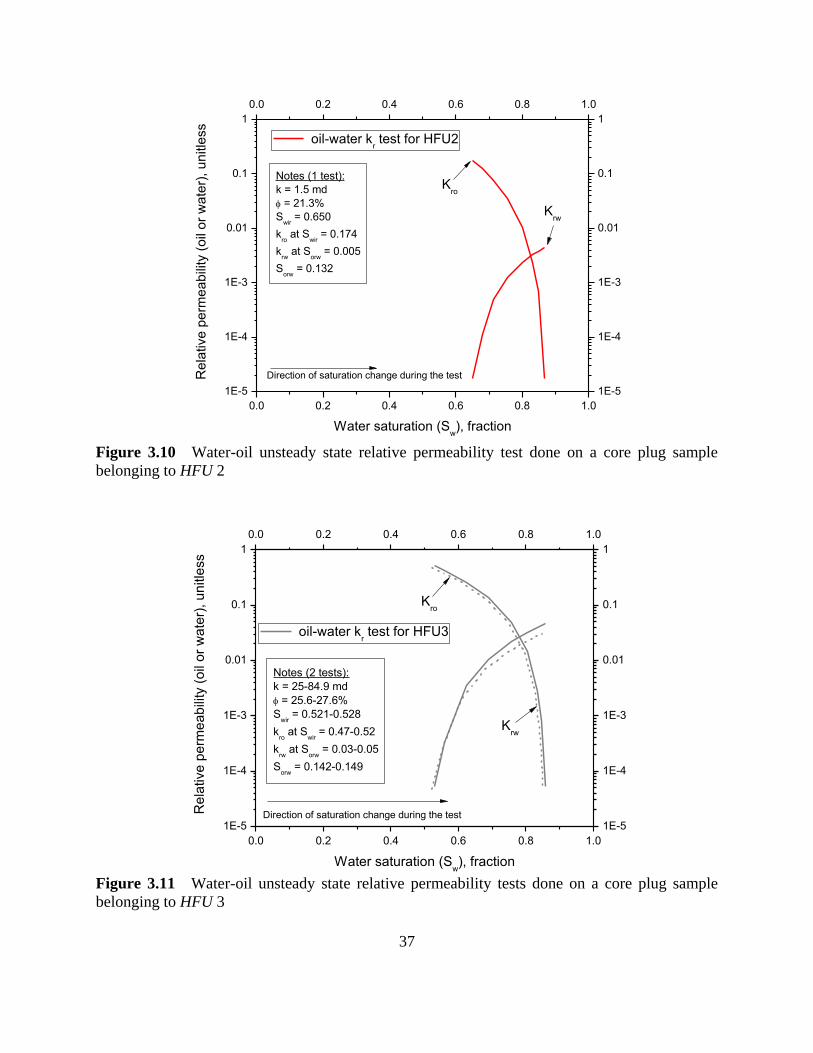
An observation from Figures 3.11 and 3.13 is that, within a given HFU, water-oil relative
permeability characteristics are very similar, varying only for rather large changes in absolute
permeability.
Table 3.3 shows the experimental microscopic displacement efficiencies at residual oil
saturation (EDmax) for each test. EDmax was estimated from Equation 3.9 (Satter et al [2008]).
𝐸𝐷𝑚𝑎𝑥 =1−𝑆𝑤𝑖𝑟−𝑆𝑜𝑟𝑤
1−𝑆𝑤𝑖𝑟= 1 −
𝑆𝑜𝑟𝑤
𝑆𝑜𝑖 (3.9)
Where Sorw is the residual oil saturation after waterflood, and Soi is the initial oil saturation.
Values of EDmax in Table 3.3 reveal, as expected, that waterflood is potentially more effective in
high quality rocks such as HFU 4 and HFU 5.
Page 49
36
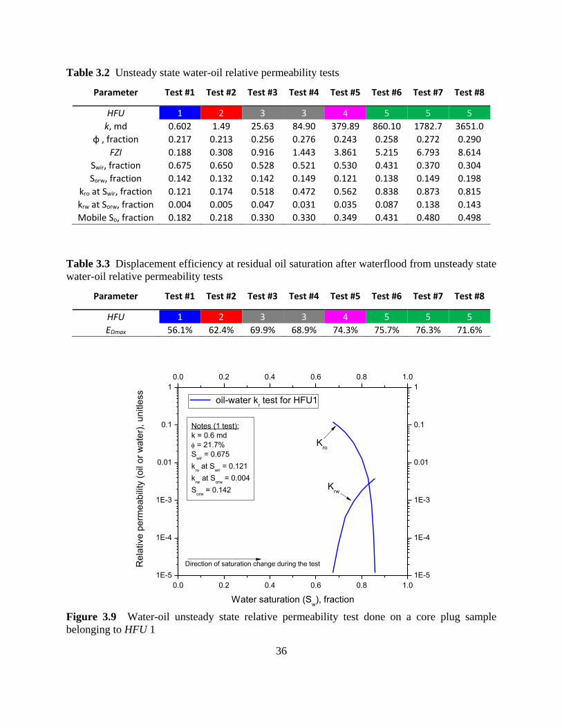
Table 3.25Unsteady state water-oil relative permeability tests
Parameter Test #1 Test #2 Test #3 Test #4 Test #5 Test #6 Test #7 Test #8
HFU 1 2 3 3 4 5 5 5
k, md 0.602 1.49 25.63 84.90 379.89 860.10 1782.7 3651.0
φ , fraction 0.217 0.213 0.256 0.276 0.243 0.258 0.272 0.290
FZI 0.188 0.308 0.916 1.443 3.861 5.215 6.793 8.614
Swir, fraction 0.675 0.650 0.528 0.521 0.530 0.431 0.370 0.304
Sorw, fraction 0.142 0.132 0.142 0.149 0.121 0.138 0.149 0.198
kro at Swir, fraction 0.121 0.174 0.518 0.472 0.562 0.838 0.873 0.815
krw at Sorw, fraction 0.004 0.005 0.047 0.031 0.035 0.087 0.138 0.143
Mobile So, fraction 0.182 0.218 0.330 0.330 0.349 0.431 0.480 0.498
Table 3.36Displacement efficiency at residual oil saturation after waterflood from unsteady state
water-oil relative permeability tests
Parameter Test #1 Test #2 Test #3 Test #4 Test #5 Test #6 Test #7 Test #8
HFU 1 2 3 3 4 5 5 5
EDmax 56.1% 62.4% 69.9% 68.9% 74.3% 75.7% 76.3% 71.6%
Figure 3.918Water-oil unsteady state relative permeability test done on a core plug sample
belonging to HFU 1
0.0 0.2 0.4 0.6 0.8 1.0
1E-5
1E-4
1E-3
0.01
0.1
1
0.0 0.2 0.4 0.6 0.8 1.0
1E-5
1E-4
1E-3
0.01
0.1
1
Krw
Re
lative
pe
rme
ab
ility
(o
il o
r w
ate
r), u
nitle
ss
Water saturation (Sw), fraction
oil-water kr test for HFU1
Kro
Direction of saturation change during the test
Notes (1 test):
k = 0.6 md
= 21.7%
Swir
= 0.675
kro at S
wir = 0.121
krw
at Sorw
= 0.004
Sorw
= 0.142
Page 50
37
Figure 3.1019Water-oil unsteady state relative permeability test done on a core plug sample
belonging to HFU 2
Figure 3.1120Water-oil unsteady state relative permeability tests done on a core plug sample
belonging to HFU 3
0.0 0.2 0.4 0.6 0.8 1.0
1E-5
1E-4
1E-3
0.01
0.1
1
0.0 0.2 0.4 0.6 0.8 1.0
1E-5
1E-4
1E-3
0.01
0.1
1
Krw
Re
lative
pe
rme
ab
ility
(o
il o
r w
ate
r), u
nitle
ss
Water saturation (Sw), fraction
oil-water kr test for HFU2
Kro
Direction of saturation change during the test
Notes (1 test):
k = 1.5 md
= 21.3%
Swir
= 0.650
kro at S
wir = 0.174
krw
at Sorw
= 0.005
Sorw
= 0.132
0.0 0.2 0.4 0.6 0.8 1.0
1E-5
1E-4
1E-3
0.01
0.1
1
0.0 0.2 0.4 0.6 0.8 1.0
1E-5
1E-4
1E-3
0.01
0.1
1
Krw
Re
lative
pe
rme
ab
ility
(o
il o
r w
ate
r), u
nitle
ss
Water saturation (Sw), fraction
oil-water kr test for HFU3
Kro
Direction of saturation change during the test
Notes (2 tests):
k = 25-84.9 md
= 25.6-27.6%
Swir
= 0.521-0.528
kro at S
wir = 0.47-0.52
krw
at Sorw
= 0.03-0.05
Sorw
= 0.142-0.149
Page 51
38
Figure 3.1221Water-oil unsteady state relative permeability test done on a core plug sample
belonging to HFU 4
Figure 3.1322Water-oil unsteady state relative permeability tests done on a core plug sample
belonging to HFU 5
0.0 0.2 0.4 0.6 0.8 1.0
1E-5
1E-4
1E-3
0.01
0.1
0.0 0.2 0.4 0.6 0.8 1.0
1E-5
1E-4
1E-3
0.01
0.1
Krw
Re
lative
pe
rme
ab
ility
(o
il o
r w
ate
r), u
nitle
ss
Water saturation (Sw), fraction
oil-water kr test for HFU3
Kro
Direction of saturation change during the test
Notes (1 test):
k = 379.9 md
= 24.3%
Swir
= 0.530
kro at S
wir = 0.562
krw
at Sorw
= 0.035
Sorw
= 0.121
0.0 0.2 0.4 0.6 0.8 1.0
1E-4
1E-3
0.01
0.1
1
0.0 0.2 0.4 0.6 0.8 1.0
1E-4
1E-3
0.01
0.1
1
Krw
Re
lative
pe
rme
ab
ility
(o
il o
r w
ate
r), u
nitle
ss
Water saturation (Sw), fraction
Kro
Direction of saturation change during the test
Notes (3 tests):
k = 860-3651md
= 25.8-29.0%
Swir
= 0.30-0.43
kro at S
wir = 0.81-0.87
krw
at Sorw
= 0.09-0.14
Sorw
= 0.138-0.198
Page 52
39
Finally, despite the evident differences in FZI among the tested samples, the amount of oil
remaining after waterflood (i.e. Sorw) is relatively invariant among all five HFU. This can be seen
in Table 3.2 and Figure 3.14. Figure 3.14 is the initial-residual saturation plot. Land [1967] and
Land [1971] showed that the residual, or trapped, saturation of a non-wetting phase is function of
its initial saturation and a parameter, called Land’s trapping constant (C). Land’s model is the
most widely used trapping model (Spiteri et al [2008]). Values of C for various formations have
been reported in the literature, with values generally lower than 5 (Blunt [2017] and van Golf-
Racht [1982]). The best estimation for a given rock however, is obtained through data fitting of
experimental data (van Golf-Racht [1982]). In Figure 3.14, experimental data was fitted with C
equal 4.5. This relationship serves as an input for numerical simulation of waterflood processes.
From given values of Soi per gridblock, Sorw is defined for all cells in the model given a known C.
Figure 3.1423Experimental initial-residual saturation plot for immiscible displacement of oil by
water
0.0 0.1 0.2 0.3 0.4 0.5 0.6 0.7 0.8 0.9 1.0
0.0
0.2
0.4
0.0 0.1 0.2 0.3 0.4 0.5 0.6 0.7 0.8 0.9 1.0
0.0
0.2
0.4
HFU 1
HFU 2
HFU 3
HFU 4
HFU 5
Fit
Re
sid
ua
l o
il a
fte
r w
ate
rflo
od
(S
orw
), fra
ctio
n
Initial oil saturation (Soi), fraction
Land [1967] relationship:
Sorw
= Soi / (1 + C*S
oi)
Parameter: C = 4.5
Experimental kr data
Page 53
40
3.5.2 Primary drainage gas-oil relative permeability data
As in the case of the water-oil system, all gas-oil relative permeability tests were run using
the unsteady state method. Core plugs were the same for both tests, but the process in this case
involves primary drainage (i.e. gas displacing oil). Table 3.4 and Figures 3.15 through 3.19
summarize the experimental data. Note that kro at Swir is the same in oil-water and gas-oil systems
(Tables 3.2 and 3.4), as this is a consistency requirement. Additionally, the final (i.e. endpoint)
gas relative permeability (krg at Sorg) is larger than krw at Sorw in Table 3.2. This is because gas is
the least wetting phase, and thus, tends to occupy the larger pores. The later remark is also evident
graphically from Figures 3.15 through 3.19 by inspection of the intersection point of the curves.
The gas saturation at which oil and gas relative permeabilities are equal is heavily displaced toward
lower gas saturation values. Also, values for EDmax in Tables 3.3 and 3.5 are remarkably similar.
Table 3.47Unsteady state gas-oil relative permeability tests
Parameter Test #1 Test #2 Test #3 Test #4 Test #5 Test #6 Test #7 Test #8
HFU 1 2 3 3 4 5 5 5
k, md 0.602 1.49 25.63 84.90 379.89 860.10 1782.7 3651.0
φ , fraction 0.217 0.213 0.256 0.276 0.243 0.258 0.272 0.290
FZI 0.188 0.308 0.916 1.443 3.861 5.215 6.793 8.614
Swir, fraction 0.675 0.650 0.528 0.521 0.530 0.431 0.370 0.304
Sorg, fraction 0.147 0.142 0.152 0.155 0.135 0.149 0.155 0.201
kro at Swir, fraction 0.121 0.174 0.518 0.472 0.562 0.838 0.873 0.815
krg at Sorg, fraction 0.17 0.030 0.188 0.163 0.211 0.252 0.417 0.356
Mobile So, fraction 0.182 0.218 0.330 0.330 0.349 0.431 0.480 0.498
Table 3.58Displacement efficiency at residual oil saturation after gas flood from unsteady state
gas-oil relative permeability tests
Parameter Test #1 Test #2 Test #3 Test #4 Test #5 Test #6 Test #7 Test #8
HFU 1 2 3 3 4 5 5 5
EDmax 54.8% 59.5% 67.8% 67.7% 71.3% 73.9% 75.3% 71.1%
Page 54
41
Figure 3.1524Gas-oil unsteady state relative permeability test done on a core plug sample
belonging to HFU1
Figure 3.1625Gas-oil unsteady state relative permeability test done on a core plug sample
belonging to HFU2
0.0 0.2 0.4 0.6 0.8 1.0
1E-5
1E-4
1E-3
0.01
0.1
0.0 0.2 0.4 0.6 0.8 1.0
1E-5
1E-4
1E-3
0.01
0.1
Krg
Re
lative
pe
rme
ab
ility
(o
il o
r g
as),
un
itle
ss
Gas saturation (Sg), fraction
gas-oil kr test for HFU1
Kro
Direction of saturation change during the test
Notes (1 test):
k = 0.6 md
= 21.7%
Swir
= 0.675
kro at S
wir = 0.121
krg at S
org = 0.017
Sorg
= 0.147
0.0 0.2 0.4 0.6 0.8 1.0
1E-5
1E-4
1E-3
0.01
0.1
1
0.0 0.2 0.4 0.6 0.8 1.0
1E-5
1E-4
1E-3
0.01
0.1
1
Krg
Re
lative
pe
rme
ab
ility
(o
il o
r g
as),
un
itle
ss
Gas saturation (Sg), fraction
gas-oil kr test for HFU2
Kro
Direction of saturation change during the test
Notes (1 test):
k = 1.5 md
= 21.3%
Swir
= 0.650
kro at S
wir = 0.174
krg at S
org = 0.030
Sorg
= 0.142
Page 55
42
Figure 3.1726Gas-oil unsteady state relative permeability tests done on a core plug sample
belonging to HFU3
Figure 3.1827Gas-oil unsteady state relative permeability test done on a core plug sample
belonging to HFU4
0.0 0.2 0.4 0.6 0.8 1.0
1E-5
1E-4
1E-3
0.01
0.1
0.0 0.2 0.4 0.6 0.8 1.0
1E-5
1E-4
1E-3
0.01
0.1
Krg
Re
lative
pe
rme
ab
ility
(o
il o
r g
as),
un
itle
ss
Gas saturation (Sg), fraction
gas-oil kr test for HFU3
Kro
Direction of saturation change during the test
Notes (2 tests):
k = 25-84.9 md
= 25.6-27.6%
Swir
= 0.521-0.528
kro at S
wir = 0.47-0.52
krg at S
org = 0.16-0.19
Sorg
= 0.152-0.155
0.0 0.2 0.4 0.6 0.8 1.0
1E-5
1E-4
1E-3
0.01
0.1
0.0 0.2 0.4 0.6 0.8 1.0
1E-5
1E-4
1E-3
0.01
0.1
Krg
Re
lative
pe
rme
ab
ility
(o
il o
r g
as),
un
itle
ss
Gas saturation (Sg), fraction
gas-oil kr test for HFU3
Kro
Direction of saturation change during the test
Notes (1 test):
k = 379.9 md
= 24.3%
Swir
= 0.530
kro at S
wir = 0.562
krg at S
org = 0.211
Sorg
= 0.135
Page 56
43
Figure 3.1928Gas-oil unsteady state relative permeability tests done on a core plug sample
belonging to HFU5
Figure 3.2029Experimental initial-residual saturation plot for immiscible displacement of oil by
gas
0.0 0.2 0.4 0.6 0.8 1.0
1E-5
1E-4
1E-3
0.01
0.1
1
0.0 0.2 0.4 0.6 0.8 1.0
1E-5
1E-4
1E-3
0.01
0.1
1
Kro
Re
lative
pe
rme
ab
ility
(o
il o
r g
as),
un
itle
ss
Gas saturation (Sg), fraction
Krg
Direction of saturation change during the test
Notes (3 tests):
k = 860-3651md
= 25.8-29.0%
Swir
= 0.30-0.43
kro at S
wir = 0.81-0.87
krg at S
org = 0.25-0.42
Sorg
= 0.149-0.1201
0.0 0.1 0.2 0.3 0.4 0.5 0.6 0.7 0.8 0.9 1.0
0.0
0.2
0.4
0.0 0.1 0.2 0.3 0.4 0.5 0.6 0.7 0.8 0.9 1.0
0.0
0.2
0.4
Fit
HFU 1
HFU 2
HFU 3
HFU 4
HFU 5
Re
sid
ua
l o
il a
fte
r g
as flo
od
(S
org),
fra
ctio
n
Initial oil saturation (Soi), fraction
Land [1967] relationship:
Sorg
= Soi / (1 + C*S
oi)
Parameter: C = 4.5
Experimental kr data
Page 57
44
Figure 3.20 shows the initial-residual saturation plot for the immiscible displacement of
oil by gas. Notably, the residual oil saturation after gas flood (Sorg) is similar to Sorw (Figure 3.14)5.
For this reason, a trapping constant (C) of 4.5 is also used to fit the data.
3.5.3 Primary drainage oil-water capillary pressure data
Capillary pressure tests were conducted using the porous plate method. Laboratory data
was converted to reservoir conditions (Dandekar [2013]) to account for the pertinent interfacial
tension and contact angle. Table 3.6 and Figure 3.21 summarize the experimental data.
Consistency with the HFU characterization is observed. For example, in Figure 3.21, FZI
increases from right to left. Low quality HFU take their place to right in the plot, as Swir is larger.
High quality rock samples, belonging to HFU 5, also display a flatter shape toward low capillary
pressure values, suggesting their pore size distribution is relatively homogeneous. Conversely,
lower quality rocks, such as HFU 2, display a non-flat capillary pressure curve, indicating higher
heterogeneity and lower grain sorting (Archer and Wall [1986]). Figure 3.22 shows the
relationship between Swir and rock permeability from all experiments (relative permeability and
capillary pressure). As rock permeability (and thus FZI) increases, Swir consistently decreases.
Table 3.69Oil-water capillary pressure tests
Parameter Test #1 Test #2 Test #3 Test #4 Test #5 Test #6 Test #7 Test #8
HFU 2 2 3 3 4 5 5 5
k, md 3.560 4.320 58.400 83.900 596.00 2549.0 3050.0 4931.0
φ , fraction 0.237 0.229 0.260 0.265 0.303 0.334 0.342 0.351
FZI 0.391 0.461 1.337 1.549 3.197 5.461 5.761 6.882
Swir, fraction 0.696 0.612 0.558 0.497 0.409 0.354 0.324 0.315
5 This is, most likely, because the capillary numbers (Nvc) involved in the displacement of oil by water and the
displacement of oil by gas did not differ enough to cause a significant change in desaturation of oil from the samples.
Nvc is a dimensionless ratio of viscous to local capillary forces (Lake et al [2014]).
Page 58
45
Figure 3.2130Oil-water capillary pressure tests at reservoir conditions
Figure 3.2231Relationship between experimental irreducible water saturation and rock
permeability
0.0 0.1 0.2 0.3 0.4 0.5 0.6 0.7 0.8 0.9 1.0
0
5
10
15
20
250.0 0.1 0.2 0.3 0.4 0.5 0.6 0.7 0.8 0.9 1.0
0
5
10
15
20
25
Direction of decreasing Swir
FZI = 6.882
Pri
ma
ry d
rain
ag
e o
il-w
ate
r
ca
pill
ary
pre
ssu
re (
Pco
w),
psig
Water saturation (Sw), fraction
HFU 2
HFU 3
HFU 4
HFU 5
Experimental data
at reservoir conditions
FZI = 0.391
Increasing FZI
0.2 0.3 0.4 0.5 0.6 0.7 0.8
10-1
100
101
102
103
1040.2 0.3 0.4 0.5 0.6 0.7 0.8
10-1
100
101
102
103
104
FZI = 0.188
HFU 1
HFU 2
HFU 3
HFU 4
HFU 5
Ro
ck p
erm
ea
bili
ty, m
d
Irreducible water saturation (Swir
), fraction
kr data
Pc data
Direction of
decreasing
rock quality
FZI = 6.882
Page 59
46
3.6 General Sedimentological Features
Fluid flow through porous media is significantly controlled by pore-throat geometrical
attributes (Abbaszadeh et al [1996]). These in turn respond to mineralogy (e.g. clay content and
distribution6, matrix and cement abundance, etc.) and texture (grain size and shape, sorting,
packing, etc.). Various combinations of these properties can lead to distinct geological facies (i.e.
lithofacies) that have similar fluid transport characteristics. Therefore, HFU not often exactly
correspond to lithofacies. Moreover, HFU are seldom vertically continuous, thus boundaries of
HFU and lithofacies may differ (Cannon [2018]).
Following the work by Amaefule et al [1993], however, a link between HFU and
lithofacies was attempted. The merit in doing this is to help guide the distribution of HFU in 3D
space based on a prior facies model.
Based on an available sedimentological report7 covering about 100 ft of rock samples
distributed over 600 ft along the cored column of the producing formation, the likely depositional
environment has been described as a fluvially-dominated delta. Dikkers [1985] pointed out that
deltaic formations are a favorite habitat for hydrocarbon accumulations.
Figures 3.23 and 3.24 show thin sections and photos at different depths in the core. The
pore size increases as the rock quality, which is characterized by an FZI value, increases (Figure
3.23). Remarkably, HFU 5 has the largest pore-throat aperture in thin sections. This explains why
the relative permeability curves (Figures 3.13 and 3.19) display high end point values, low
irreducible water saturations (Swir), and a broader range of saturations over which two phase flow
6 Types of clay distribution include structural, laminar and disperse (Schon [2011]). 7 Source is held confidential.
Page 60
47
occurs. Conversely, HFU1 has the smallest pore throats, and this causes the relative permeability
curves to have the lowest end point values and highest Swir (Figures 3.9 and 3.15). In general,
pore sizes and pore-throat aperture monotonically increase from HFU1 through HFU5 while Swir
monotonically decreases. This can be observed by naked eye from the color of the rock samples
shown in Figure 3.24, and also explains the relationship shown in Figure 3.22.
Figure 3.2332Thin sections for three of the five hydraulic from units: HFU2 (a), HFU3 (b) and
HFU5 (c) (figures a, b and c printed with permission from Zeus OL Peru SAC [2016])
0.0 0.2 0.4
10-5
10-4
10-3
10-2
10-1
100
101
102
103
104
105
0.0 0.2 0.4
10-5
10-4
10-3
10-2
10-1
100
101
102
103
104
105
Legend:
HFU5 (FZI = 7.09)
HFU4 (FZI = 2.50)
HFU3 (FZI = 1.11)
HFU2 (FZI = 0.46)
HFU1 (FZI = 0.17)
Core data
Outliers
Str
esse
d h
ori
zo
nta
l p
erm
ea
bili
ty (
kh),
md
Stressed porosity (), fraction
Notes:
Confinment 1,330 psi
0.3 mm0.6 mm 0.6 mm
HFU 5: Medium to coarse sandstones.Well sorted and poorly consolidated
HFU 2: Very fine grained sandstones andsiltstones
HFU 3: moderately sorted finesandstones
Direction of increasing rock quality (i.e. FZI)
Average FZI = 0.46 Average FZI = 1.11 Average FZI = 7.09
(a) (b) (c)
Page 61
48
Figure 3.2433Core photos showing variations in rock texture (figures a through e printed with
permission from Zeus OL Peru SAC [2016])
Hydraulic flow unit HFU1 corresponds, in general, to intercalated claystones and
siltstones. Rocks exhibit finely laminated to massive sedimentary structures (Figure 3.24a).
Deposition likely occurred in a low-energy environment, described as a subaqueous interlobe area.
For all practical purposes, these rocks act as a flow baffle or flow barrier.
Rocks characterized as HFU2, on the other hand, have been described as very fine grained
sandstones, silty sandstones and sandy siltstones. They generally exhibit massive (Figure 3.24b)
or laminated sedimentary structures with moderate bioturbation.
HFU3 tends to comprise moderately sorted, fine and coarse sandstones (Figure 3.24c).
Rocks have been described as locally calcareous, having clayey cement and presence of clasts, as
a result of episodic changes in fluvial sediment supply.
Direction of increasing rock quality (i.e. FZI)
HFU 1
k = 0.01 mdφ = 0.002FZI = 0.31
k = 2.40φ = 0.21FZI = 0.40
k = 137.12φ = 0.229FZI = 2.6
k = 16.96φ = 0.224FZI = 0.95
k = 3530.9φ = 0.334FZI = 6.44
HFU 2 HFU 3 HFU 4 HFU 5
(a) (b) (c) (d) (e)
1 ft
Page 62
49
Rocks within HFU4 include very well sorted sandstones and locally calcareous sandstones
having, in general, massive sedimentary structures (Figure 3.24d). This flow unit also includes
conglomerates, having volcanic clasts and bioclasts8, likely transported by strong fluvial currents.
Finally, rocks characterized as HFU5 have been described as medium to coarse and very
coarse grained sandstones. They are well sorted and generally poorly consolidated. Bioturbation
is scarce but not absent. These characteristics are suggestive of a high-energy landward
environment.
3.7 Summary
From available core data, which covers more than 800 ft of rock, five hydraulic flow units
(named HFU1 through HFU5) were identified. This analysis was done in an objective manner by
use of hierarchical cluster analysis. The implementation was done in the form of a MATLAB
code. The algorithm automatically determined the optimum number of flow units and their
associated FZI values. Distinct permeability-porosity relationships were defined for each flow
unit. These relationships allow to estimate permeability in uncored, but logged wells, given known
values of FZI and porosity.
The resulting flow units were also associated rock-fluid properties, such as relative
permeability and capillary pressure, obtained from experimental analysis. Consistency was
observed, for example, it was noted that as rock quality increases from HFU1 to HFU5, Swir
monotonically decreases and relative permeability end points monotonically increase. Finally,
major sedimentological features were recognized for each flow unit.
8 Sediments from organic materials (e.g. bivalve fragments).
Page 63
50
CHAPTER IV
SUMMARY AND RECOMMENDATIONS
4.1 Summary
In this study, a reservoir fluid and rock characterization was done for a Peruvian oil
reservoir. The following are major summarizing remarks:
a. Lack of PVT data from actual fluid samples was overcome by integrating analog PVT
studies, production and pressure data, well logs, and reliable fluid property correlations,
such as those in McCain et al [2011].
b. Analog fluid samples were validated by comparison of experimental and theoretical
equilibrium ratios, or k-factors. Fluid samples were deemed as valid since the sampled
gas and liquid were in equilibrium at the time of sampling.
c. Laboratory work done on analog fluid samples was also validated through the
application of a robust workflow originally proposed by Professor William D. McCain,
Jr. at Texas A&M University. In this approach, laboratory data is compared against
reliable fluid property correlations, such as those in McCain et al [2011]. Agreement
was observed, indicating that the laboratory work was valid.
d. The resulting fluid model was a black-oil variable bubble point model, in which internal
consistencies of gas and oil properties were checked by ensuring that the oil
compressibility (co) remained positive throughout the range of extrapolated pressures.
e. Five hydraulic flow units (named HFU1 through HFU5) were identified from core
samples spanned along more than 800 ft. This analysis was done in an objective
Page 64
51
manner by use of hierarchical cluster analysis. The implementation was done in the
form of a MATLAB code. The algorithm automatically determined the optimum
number of flow units and their associated FZI values.
f. The hydraulic flow units (HFU) were associated rock-fluid properties, such as relative
permeability and capillary pressure, obtained from experimental analysis. Consistency
was observed, for example, it was noted that as rock quality increases from HFU1 to
HFU5, Swir monotonically decreased and relative permeability end points
monotonically increased.
g. Major sedimentological features were recognized for each flow unit. For instance,
HFU1 corresponded, in general, to intercalated claystones and siltstones, and for all
practical purposes, it acts as a flow baffle or flow barrier.
4.2 Recommendations
a. Automatic outlier detection could be implemented in the MATLAB code for
hierarchical cluster analysis of hydraulic flow units.
b. Incorporate a piece of code to automatically determine the change of slope in the elbow
method (Figure 3.6).
c. Study the applicability of model-based cluster analysis, such as the expectation-
maximization (EM) algorithm, as an alternative way to define hydraulic flow units.
Page 65
52
REFERENCES
Abbaszadeh, M., Fujii, H., and Fujimoto, F. 1996. Permeability Prediction by Hydraulic Flow
Units - Theory and Applications. Society of Petroleum Engineers. doi:10.2118/30158-PA.
Amaefule, J.O., Altunbay, M., and Tiab, D. 1993. Enhanced Reservoir Description: Using Core
and Log Data to Identify Hydraulic (Flow) Units and Predict Permeability in Uncored
Intervals/Wells. Presented at the 68th Annual Technical Conference and Exhibition of the
Society of Petroleum Engineers, Houston, Texas, 03—06 October. SPE-26436.
http://dx.doi.org/10.2118/26436.
Archer, J. and Wall, C. 1986. Petroleum Engineering: Principles and Practice. London: Graham
& Trotman.
Baker, R.O., Yarranton, H.W. and Jensen, J.L. 2015. Practical reservoir engineering and
characterization. Waltham, MA: Gulf Professional Publishing is an imprint of Elsevier.
Bear, J., 1972. Dynamics of Fluids in Porous Media. Elsevier, New York.
Blunt, M. 2017. Multiphase Flow in Permeable Media: a Pore-Scale Perspective. Cambridge,
United Kingdom New York, NY: Cambridge University Press.
Bruno, I.A., Yanosik, I.L., and Tierney, I.W. 1972. Distillation Calculations with Nonideal
Mixtures. In Extractive and Aziotropic Distillation. Advances in Chemistry Series 115,
ACS, Washington, DC.
Cannon, S. 2018. Reservoir Modelling: a Practical Guide. Hoboken, NJ: Wiley.
Carman, P. C. 1961. L’e’coulement des Gaz a´ Travers les Milieux Poreux: Bibliothe’que des
Sciences et Techniques Nucle’aires: Presses Universitaires de France.
Dandekar, A.Y. 2013. Petroleum Reservoir Rock and Fluid Properties. Boca Raton, FL: CRC
Press.
Dake, L. P. 1978. Fundamentals of reservoir engineering. Amsterdam; New York; New York:
Elsevier Scientific Pub. Co.; Distributors for the U.S. and Canada Elsevier North-Holland.
Dezfoolian, M., Riahi, M.and Kadkhodaie, A. 2013. Conversion of 3D seismic attributes to
reservoir hydraulic flow units using a neural network approach: An example from the
Kangan and Dalan carbonate reservoirs, the world’s largest non-associated gas reservoirs,
near the Persian Gulf. Earth Sciences Research Journal. 17. 75-85.
Dikkers, A. 1985. Geology in Petroleum Production: a Primer in Production Geology.
Amsterdam New York: Elsevier.
Ebanks W.J. 1987. Flow Unit Concept — Integrated Approach to Reservoir Description for
Engineering Projects (abs.). American Association of Petroleum Geologists Bulletin 71,
551–552.
Page 66
53
Ebanks, W. J. 1992. Flow Units for Reservoir Characterization. Development Geology
Reference Manual. AAPG Methods in Exploration Series no. 10, 1992. p. 282.285.
Han, J., Kamber, M. and Pei, J. 2012. Data Mining: Concepts and Techniques. Amsterdam;
Boston: Elsevier/Morgan Kaufmann.
Hoffman, A. E., Crump, J. S., and Hocott, C. R. 1953. Equilibrium Constants for a Gas-
Condensate System. Society of Petroleum Engineers. doi:10.2118/219-G.
Lake, L.W., Johns, R., Rossen, B. and Pope, G. 2014. Fundamentals of enhanced oil recovery.
Richardson, Tex.: Society of Petroleum Engineers.
Land, C. 1967. Calculation of Imbibition Relative Permeability for Two- and Three Phase Flow
From Rock Properties. Presented at the SPE 42nd Annual Fall Meeting, Houston, Texas,
01—04 October. SPE-1942. http://dx.doi.org/10.2118/1942.
Land, C. 1971. Comparison of Calculated with Experimental Imbibition Relative Permeability.
Presented at the SPE Rocky Mountain Regional Meeting, Houston, Texas, 02—04 June.
SPE-1942. http://dx.doi.org/10.2118/1942.
McCain, W.D. 1990. The Properties of Petroleum Fluids, second edition. PennWell.
McCain, W. D. and Spivey, J. P. 1999. Extrapolation of Laboratory Measured Black Oil and
Solution Gas Fluid Properties for Variable Bubble Point Simulation. Society of Petroleum
Engineers. doi:10.2118/56746-MS.
McCain, W.D., Spivey, J., and Lenn, C.P. 2011. Petroleum Reservoir Fluid Property
Correlations, first edition. Tulsa, Oklahoma: PennWell.
McCain, W.D. 2016. Careful Sampling – Why Do We Care? [Class handout]. College Station,
Texas: Texas A&M University, PETE-605.
McCain, W.D. (2018, January 8). Personal communication.
Pedersen, K.S., Christensen, P.L., and Shaikh, J.A. 2015. Phase Behavior of Petroleum Reservoir
Fluids, second edition. CRC Press.
Satter, A., Iqbal, G.M. and Buchwalter, J.L. 2008. Practical enhanced reservoir engineering:
assisted with simulation software. Tulsa, Okla.: PennWell Corp.
Schlumberger. 2015. ECLIPSE Reference Manual 2015.1. Schlumberger Information
Solutions, Houston.
Schon, J. 2011. Physical Properties of Rocks: a Workbook. Amsterdam: Elsevier.
Slider, H.C. 1983. Worldwide Practical Petroleum Reservoir Engineering Methods: PennWell
Books.
SPE. 2018. Petrowiki by Society of Petroleum Engineers (SPE). Relative Permeability Models,
http://petrowiki.org/Relative_permeability_models (accessed 15 February 2018).
Page 67
54
Spiteri, E. J., Juanes, R., Blunt, M. J., and Orr, F. M. 2008. A New Model of Trapping and
Relative Permeability Hysteresis for All Wettability Characteristics. Society of Petroleum
Engineers. doi:10.2118/96448-PA.
Stolz, A.-K., and Graves, R. M. 2003. Sensitivity Study of Flow Unit Definition by Use of
Reservoir Simulation. Society of Petroleum Engineers. doi:10.2118/84277-MS.
Svirsky, D., Ryazanov, A., Pankov, M., Corbett, P. W. M., and Posysoev, A. 2004. Hydraulic
Flow Units Resolve Reservoir Description Challenges in a Siberian Oil Field. Society of
Petroleum Engineers. doi:10.2118/87056-MS.
Tiab, D. and Donaldson, E.C. 2016. Petrophysics: Theory and Practice of Measuring Reservoir
Rock and Fluid Transport Properties, fourth edition. Amsterdam: Gulf Professional
Publishing, an imprint of Elsevier.
van Golf-Racht, T.D. 1982. Fundamentals of fractured reservoir engineering. Amsterdam; New
York: Elsevier.
Wattenbarger, R.A. 2000. Repressuring with Variable Bubble Point [Class handout]. College
Station, Texas: Texas A&M University, PETE-611.
Zeus OL Peru SAC. 2016. Sedimentological descriptions. Unpublished internal document.
Page 68
55
APPENDIX A
This appendix reproduces relevant fluid property correlations in McCain et al [2011]. Oil
density at pressures equal or less than the bubble point are calculated from Equations A.1 through
A.6 (McCain et al [2011]):
𝜌𝑜𝑅 = [𝑅𝑆 𝛾𝑔+4600 𝛾𝑆𝑇𝑂
73.71+𝑅𝑆 𝛾𝑔
𝜌𝑎⁄
] + ∆𝜌𝑝 − ∆𝜌𝑇 (A.1)
𝜌𝑎 = 𝑎0 + 𝑎1𝛾𝑔𝑆𝑃 + 𝑎2𝛾𝑔𝑆𝑃𝜌𝑝𝑜 + 𝑎3𝛾𝑔𝑆𝑃𝜌𝑝𝑜2 + 𝑎4𝜌𝑝𝑜 + 𝑎5𝜌𝑝𝑜
2 (A.2)
∆𝜌𝑝 =[0.167+16.181(10−0.0425𝜌𝑝𝑜)]
(1000
𝑃)
− 0.01[0.299 + 263(10−0.0603𝜌𝑝𝑜)] (𝑃
1000)
2 (A.3)
∆𝜌𝑇 =(0.00302+
1.505
(𝜌𝑝𝑜+∆𝜌𝑝)0.951)
(𝑇−60)−0.938 −
[0.0216−0.0233
(10−0.0161(𝜌𝑝𝑜+∆𝜌𝑝)
)]
(𝑇−60)−0.475 (A.4)
Where γSTO is the stock-tank oil specific gravity; ρa is an apparent liquid density, and Δρp
and ΔρT are pressure and temperature corrections.
In Equation A.2 coefficients are as follows: a0 = -49.8930; a1 = 85.0149; a2 = -3.70373; a3
= 0.0479818; a4 = 2.98914; a5 = -0.0356888.
Equations A.1 through A.4 require iteration on ρpo, for which the first trial value is given
as:
𝜌𝑝𝑜 = 52.8 − 0.01𝑅𝑠 (A.5)
At pressures greater than the bubble point, the oil density is found from the oil
compressibility:
Page 69
56
𝜌𝑜𝑅 = 𝜌𝑜𝑅𝑏 ∙ 𝑒[𝐶𝑜𝑓𝑏(𝑃−𝑃𝑏)] (A.6)
Where ρoRb is the oil density at the bubble point, and Cofb is the coefficient of isothermal
compressibility of oil at pressures greater than the bubble point. Cofb is found from equation 3.13
in McCain et al [2011].
The bubble point pressure (Pb) at a given reservoir temperature (TR) and at a specified
solution gas-oil ratio at the bubble point (RSB) is calculated from Equations A.7 through A.9:
𝑙𝑛(𝑃𝐵) = 7.475 + 0.713𝑍 + 0.0075𝑍2 (A.7)
𝑍 = ∑ 𝑍𝑛4𝑛=1 (A.8)
𝑍𝑛 = 𝐶0𝑛 + 𝐶1𝑛𝑉𝐴𝑅𝑛 + 𝐶2𝑛𝑉𝐴𝑅𝑛2 + 𝐶3𝑛𝑉𝐴𝑅𝑛
3 (A.9)
Coefficients C0, C1, C2 and C3 for the n variables VAR are given in Table A.1:
Table A.110Coefficients in the correlation for Pb (after McCain et al [2011])
n VAR C0n C1n C2n C3n
1 ln(RSB) -5.48 -0.0378 0.281 -0.0206
2 API 1.27 -0.0449 4.36 x 10⁻⁴ -4.76 x 10⁻⁶
3 γgSP 4.51 -10.84 8.39 -2.34
4 TR -0.7835 6.23 x 10⁻³ -1.22 x 10⁻⁵ 1.03 x 10⁻⁸
The solution gas-oil ratio (RS) at reservoir pressures lower than PB is calculated from
Equations A.10 through A.13:
𝑅𝑆 = 𝑅𝑆𝐵 {𝑎1 (𝑃−14.7
𝑃𝑏−14.7)
𝑎2
+ (1 − 𝑎1) (𝑃−14.7
𝑃𝑏−14.7)
𝑎3
} (A.10)
𝑎1 = 𝐴0(𝛾𝑔𝑆𝑃)𝐴1
𝐴𝑃𝐼𝐴2𝑇𝐴3(𝑃𝐵 − 14.7)𝐴4 (A.11)
Page 70
57
𝑎2 = 𝐵0(𝛾𝑔𝑆𝑃)𝐵1
𝐴𝑃𝐼𝐵2𝑇𝐵3(𝑃𝐵 − 14.7)𝐵4 (A.12)
𝑎1 = 𝐶0(𝛾𝑔𝑆𝑃)𝐶1
𝐴𝑃𝐼𝐶2𝑇𝐶3(𝑃𝐵 − 14.7)𝐶4 (A.13)
Coefficients in Equations A.10 through A.13 are given in Table A.2.
Table A.211Coefficients in the correlation for Rs below Pb (after McCain et al [2011])
n An Bn Cn
0 9.73 x 10⁻⁷ 0.022339 0.725167
1 1.672608 -1.004750 -1.485480
2 0.929870 0.337711 -0.164741
3 0.247235 0.132795 -0.091330
4 1.056052 0.302065 0.047094
The coefficient of isothermal compressibility of oil at reservoir pressures greater than
bubble point pressure (Cofb) is calculated from Equations A.14 through A.16:
𝑙𝑛(𝐶𝑜𝑓𝑏) = 2.434 + 0.475𝑍 + 0.048𝑍2 − 𝑙𝑛(106) (A.14)
𝑍 = ∑ 𝑍𝑛6𝑛=1 (A.15)
𝑍𝑛 = 𝐶0𝑛 + 𝐶1𝑛𝑉𝐴𝑅𝑛 + 𝐶2𝑛𝑉𝐴𝑅𝑛2 (A.16)
Coefficients in Equations A.14 through A.16 for the n variables VAR are in Table A.3:
Table A.312Coefficients in the correlation for Pb (after McCain et al [2011])
n VAR C0n C1n C2n
1 ln(API) 3.011 -2.6254 0.497
2 ln(γgSP) -0.0835 -0.259 0.382
3 ln(Pb) 3.51 -0.0289 -0.0584
4 ln(P/Pb) 0.327 -0.608 0.0911
5 ln(Rsb) -1.918 -0.642 0.154
6 ln(TR) 2.52 -2.73 0.429
Page 71
58
The oil formation volume factor at reservoir pressures equal to and less than PB (Bo) is
found from Equation 2.3. At pressures greater than PB, Bo is given by Equation A.17:
𝐵𝑜 = 𝐵𝑜𝑏 ∙ 𝑒[𝐶𝑜𝑓𝑏(𝑃−𝑃𝑏)] (A.17)
Equation A.17 is not a correlation. It follow directly from the definition of the coefficient
of isothermal compressibility of oil.