167
Resetting uncontrolled quantum systems Institute for Quantum Optics and Quantum Information (IQOQI), Vienna Miguel Navascués MN, arXiv:1710.02470
Resetting uncontrolled quantum systems
Institute for Quantum Optics and Quantum Information (IQOQI), Vienna
Miguel Navascués
MN, arXiv:1710.02470
I invented a time-warping device,
ask me how!
Institute for Quantum Optics and Quantum Information (IQOQI), Vienna
Miguel Navascués
MN, arXiv:1710.02470
Definition of TIME-WARP
noun | \ ˈtīm ˈwȯrp \
Time-warp
1. an anomaly, discontinuity, or suspension held to occur in the progress of time

𝑡 = 0
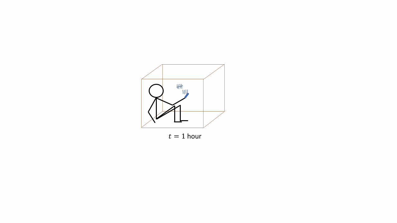
𝑡 = 1 hour
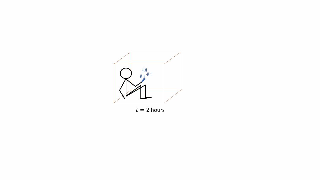
𝑡 = 2 hours

𝑡 = 0
𝑡 = 0
Time warp for two hours
𝑡 = 2 hours
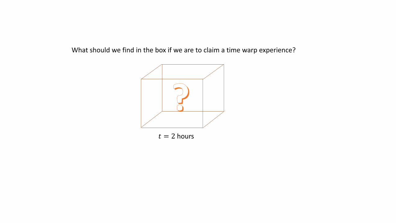
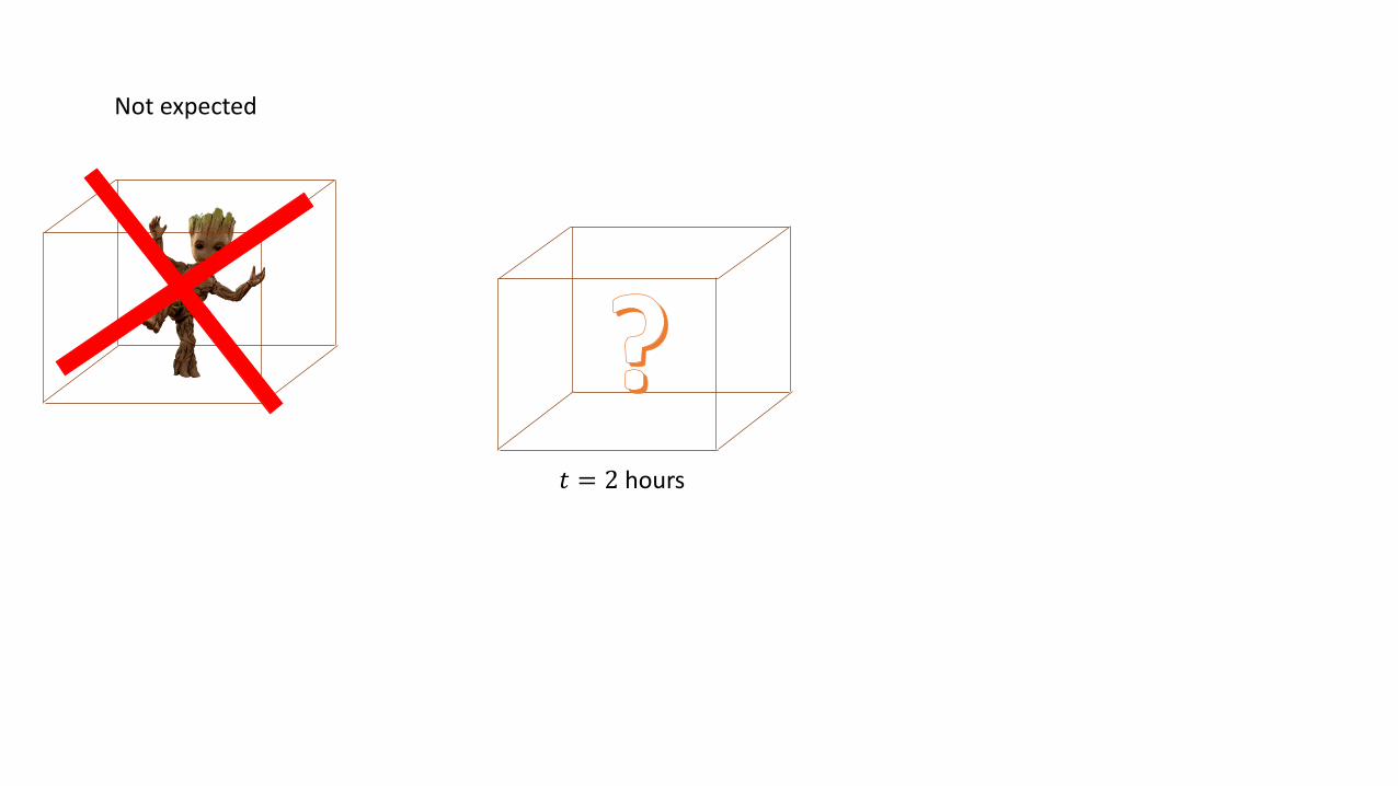
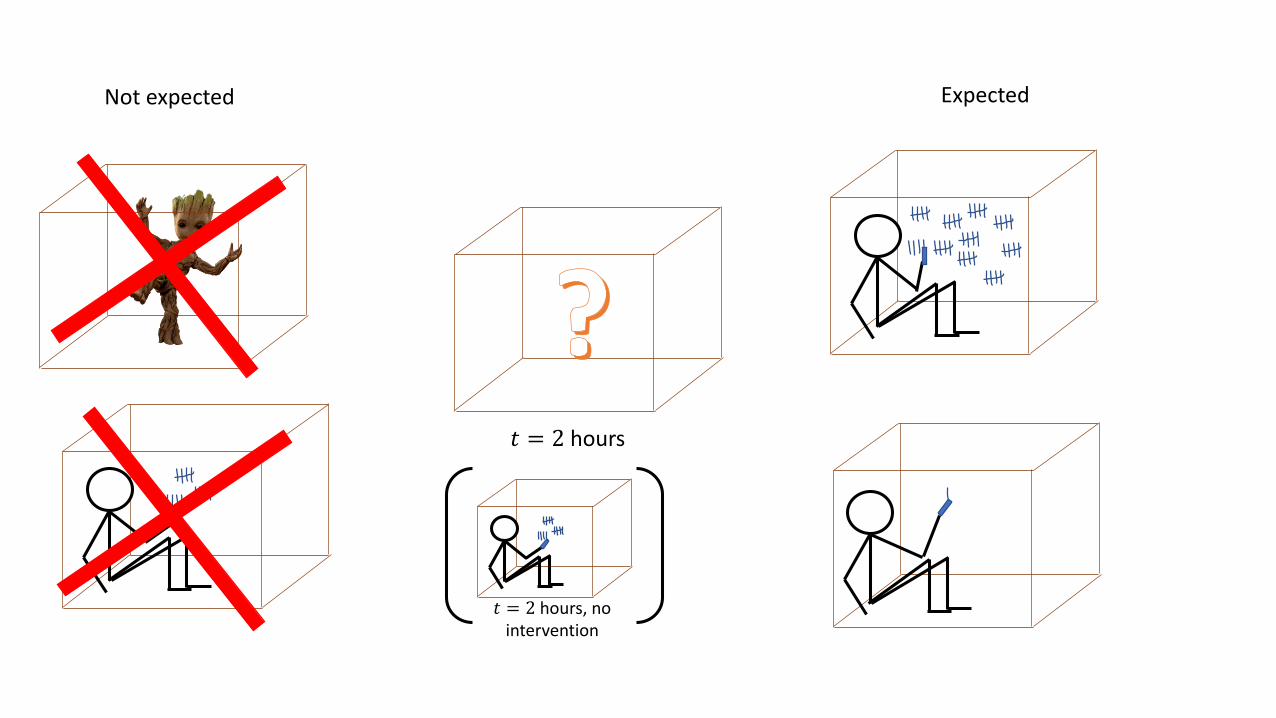
What should we find in the box if we are to claim a time warp experience?
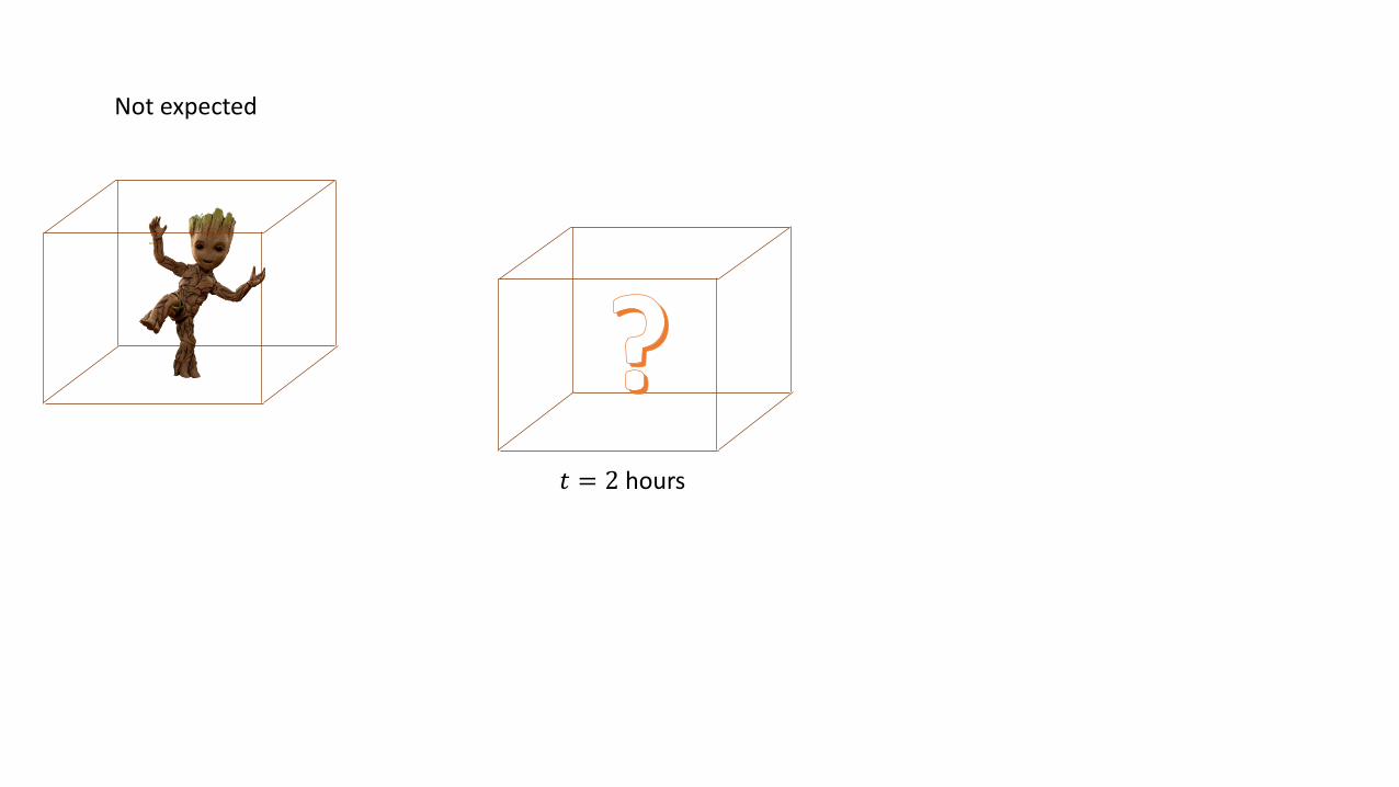
Not expected
𝑡 = 2 hours
𝑡 = 2 hours
Not expected
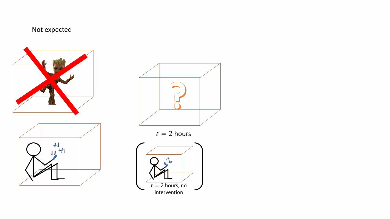
𝑡 = 2 hours
Not expected
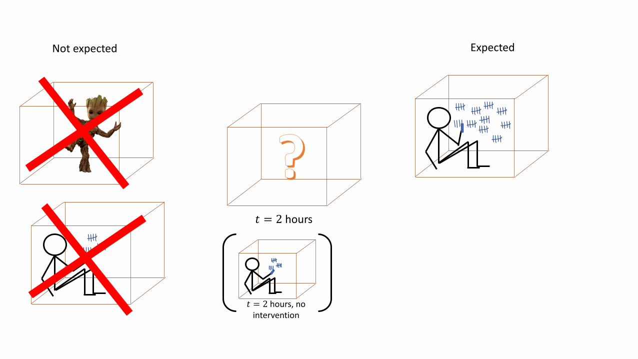
𝑡 = 2 hours, no intervention
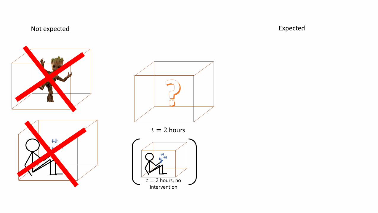
Expected
𝑡 = 2 hours
Not expected
𝑡 = 2 hours, no intervention
Expected
𝑡 = 2 hours
Not expected
𝑡 = 2 hours, no intervention
𝑡 = 2 hours
ExpectedNot expected
𝑡 = 2 hours, no intervention
{𝜓 𝑡 : 𝑡}
Time warp: operational definition
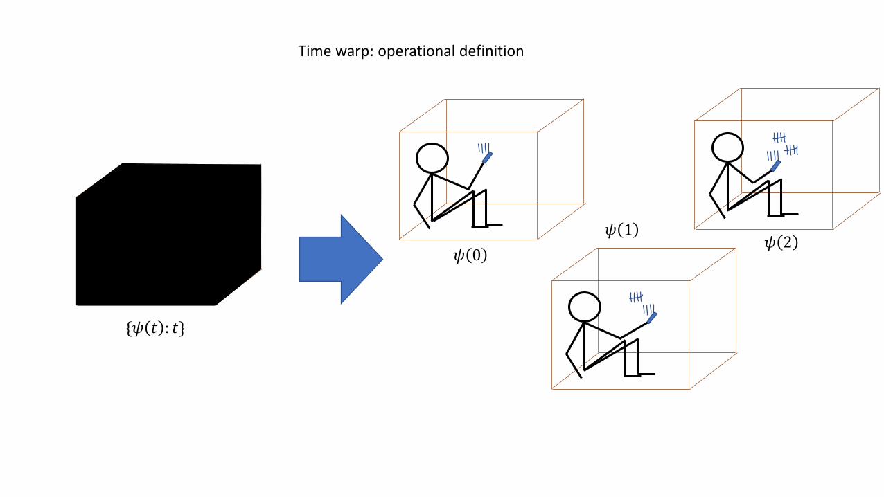
{𝜓 𝑡 : 𝑡}
𝜓 0
𝜓 1𝜓 2
Time warp: operational definition
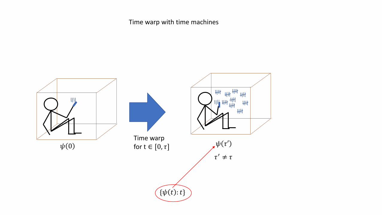
Time warp protocol for t ∈ [0, 𝜏]
Time warp: operational definition
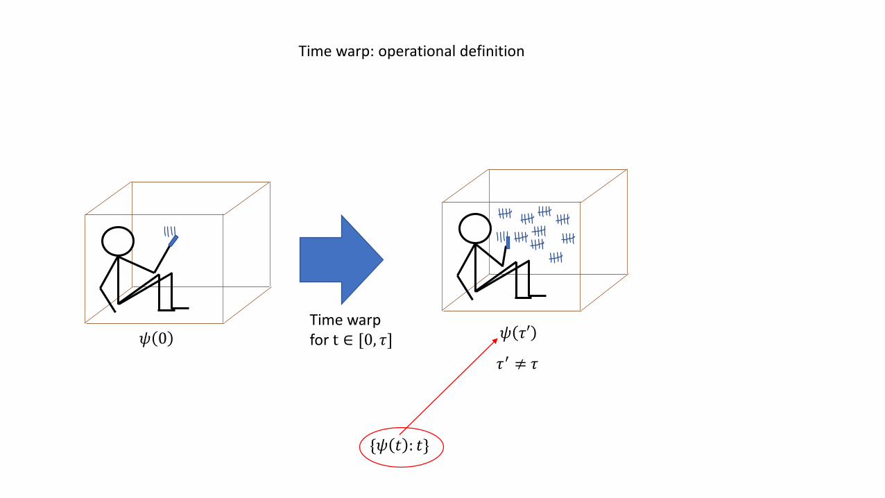
𝜓 𝜏′
𝜏′ ≠ 𝜏
Time warp: operational definition
{𝜓 𝑡 : 𝑡}
𝜓 0Time warpfor t ∈ [0, 𝜏]

A brief history of time warp

King Raivata and princess Revati
(400BC?)

Peter Damian(1007-1072)

(first edition in 1895)

Warping time physically

𝜓 𝜏′
0 < 𝜏′ < 𝜏
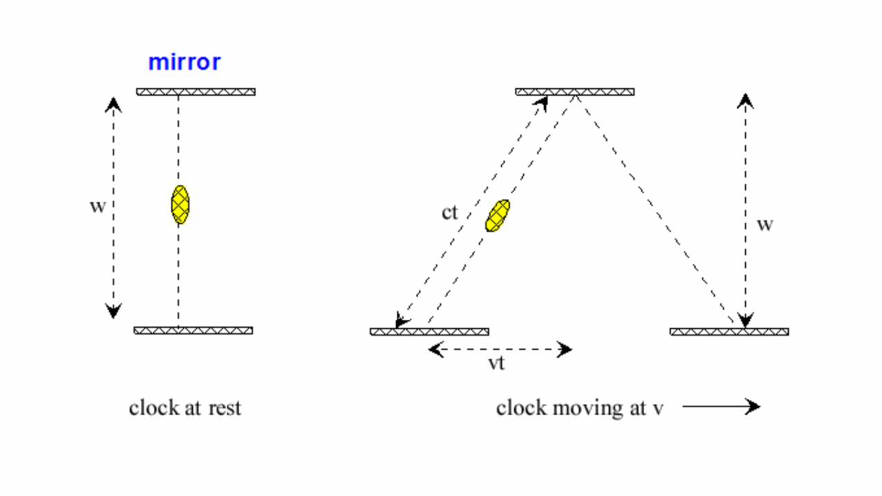
Time warp in special relativity
{𝜓 𝑡 : 𝑡}
𝜓 0Time warpfor t ∈ [0, 𝜏]
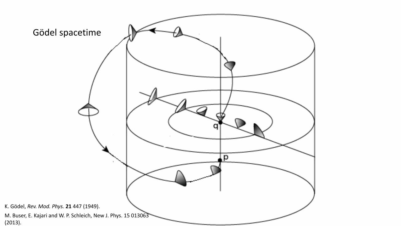
Gödel spacetime
M. Buser, E. Kajari and W. P. Schleich, New J. Phys. 15 013063 (2013).
K. Gödel, Rev. Mod. Phys. 21 447 (1949).
Time travelwith
wormholes
K. Thorne, Black Holes and Time Warps: Einstein'sOutrageous Legacy, Commonwealth Fund Book Program(1994).
𝜓 𝜏′
𝜏′ ≠ 𝜏
Time warp with time machines
{𝜓 𝑡 : 𝑡}
𝜓 0Time warpfor t ∈ [0, 𝜏]
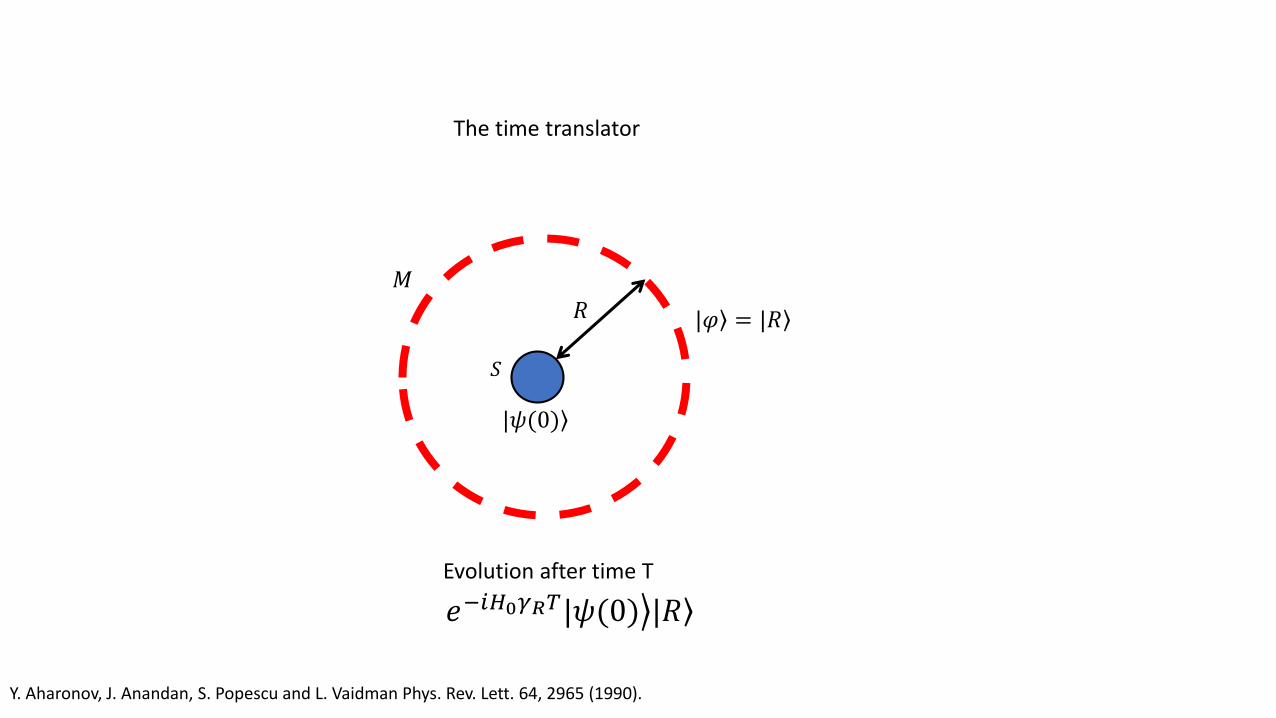
Y. Aharonov, J. Anandan, S. Popescu and L. Vaidman Phys. Rev. Lett. 64, 2965 (1990).
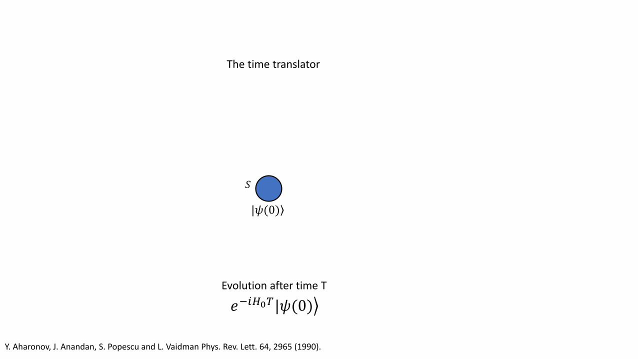
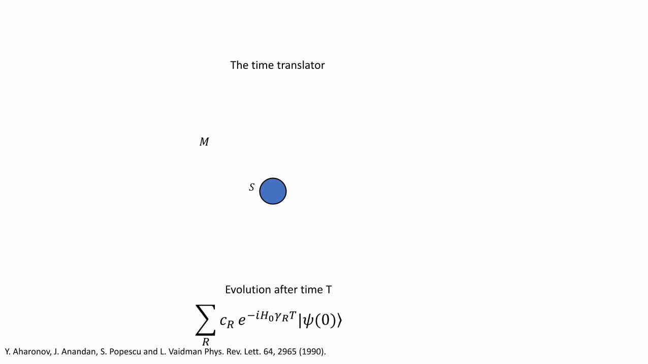
The time translator
ൿ𝑒−𝑖𝐻0𝑇|𝜓(0)
Evolution after time T
𝑆
|𝜓(0)
Y. Aharonov, J. Anandan, S. Popescu and L. Vaidman Phys. Rev. Lett. 64, 2965 (1990).
The time translator
𝑆
𝑅
𝑀
ൿ𝑒−𝑖𝐻0𝛾𝑅𝑇|𝜓(0) |𝑅
Evolution after time T
|𝜑 = |𝑅
|𝜓(0)
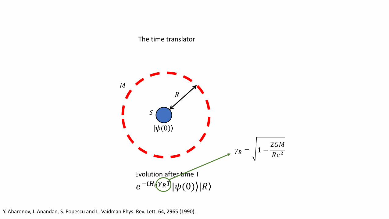
ൿ𝑒−𝑖𝐻0𝛾𝑅𝑇|𝜓(0) |𝑅
Y. Aharonov, J. Anandan, S. Popescu and L. Vaidman Phys. Rev. Lett. 64, 2965 (1990).
The time translator
𝑆
𝑅
𝑀
Evolution after time T
𝛾𝑅 = 1 −2𝐺𝑀
𝑅𝑐2
|𝜓(0)
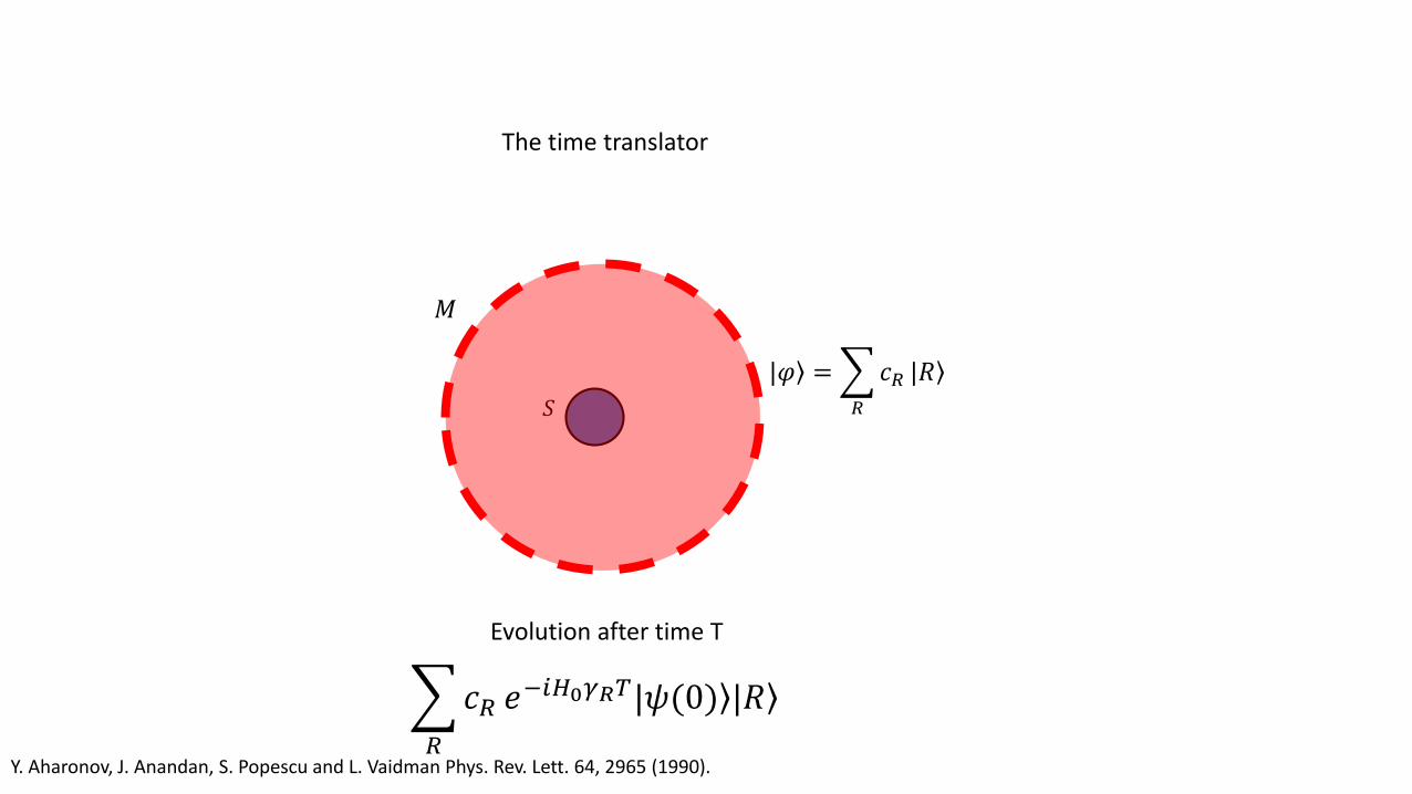
Y. Aharonov, J. Anandan, S. Popescu and L. Vaidman Phys. Rev. Lett. 64, 2965 (1990).
The time translator
𝑆
𝑀
𝑅
𝑐𝑅 𝑒−𝑖𝐻0𝛾𝑅𝑇 |𝜓(0) |𝑅
Evolution after time T
|𝜑 =
𝑅
𝑐𝑅 |𝑅
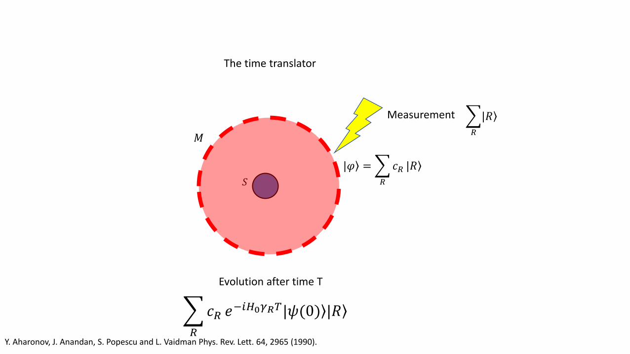
Y. Aharonov, J. Anandan, S. Popescu and L. Vaidman Phys. Rev. Lett. 64, 2965 (1990).
The time translator
𝑆
𝑀
Evolution after time T
|𝜑 =
𝑅
𝑐𝑅 |𝑅
Measurement
𝑅
|𝑅
𝑅
𝑐𝑅 𝑒−𝑖𝐻0𝛾𝑅𝑇 |𝜓(0) |𝑅
Y. Aharonov, J. Anandan, S. Popescu and L. Vaidman Phys. Rev. Lett. 64, 2965 (1990).
The time translator
𝑆
𝑀
𝑅
𝑐𝑅 𝑒−𝑖𝐻0𝛾𝑅𝑇 |𝜓(0)
Evolution after time T
Y. Aharonov, J. Anandan, S. Popescu and L. Vaidman Phys. Rev. Lett. 64, 2965 (1990).
The time translator
𝑆
𝑀
𝑅
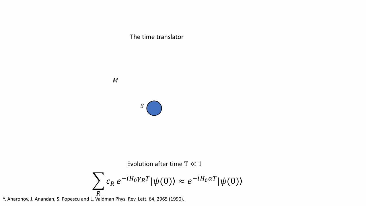
𝑐𝑅 𝑒−𝑖𝐻0𝛾𝑅𝑇 |𝜓(0) ≈ 𝑒−𝑖𝐻0𝛼𝑇 |𝜓(0)
Evolution after time T ≪ 1
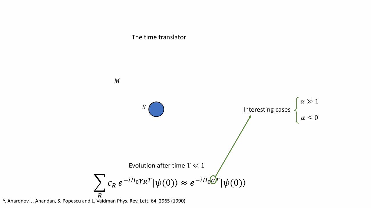
Y. Aharonov, J. Anandan, S. Popescu and L. Vaidman Phys. Rev. Lett. 64, 2965 (1990).
The time translator
𝑆
𝑀
𝑅
𝑐𝑅 𝑒−𝑖𝐻0𝛾𝑅𝑇 |𝜓(0) ≈ 𝑒−𝑖𝐻0𝛼𝑇 |𝜓(0)
Evolution after time T ≪ 1
𝛼 ≫ 1
𝛼 ≤ 0Interesting cases

𝜓 𝜏′
𝜏′ ≠ 𝜏
Time warp with the time translator
{𝜓 𝑡 : 𝑡}
𝜓 0Time warpfor t ∈ [0, 𝜏]
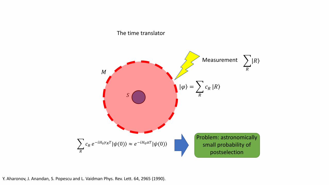
Y. Aharonov, J. Anandan, S. Popescu and L. Vaidman Phys. Rev. Lett. 64, 2965 (1990).
The time translator
𝑆
𝑀
|𝜑 =
𝑅
𝑐𝑅 |𝑅
Measurement
𝑅
|𝑅
Problem: astronomicallysmall probability of
postselection
𝑅
𝑐𝑅 𝑒−𝑖𝐻0𝛾𝑅𝑇 |𝜓(0) ≈ 𝑒−𝑖𝐻0𝛼𝑇 |𝜓(0)
“The time translator has the same chances of succeeding as I have of delocalizing and
relocalizing somewhere else”
L. Vaidman
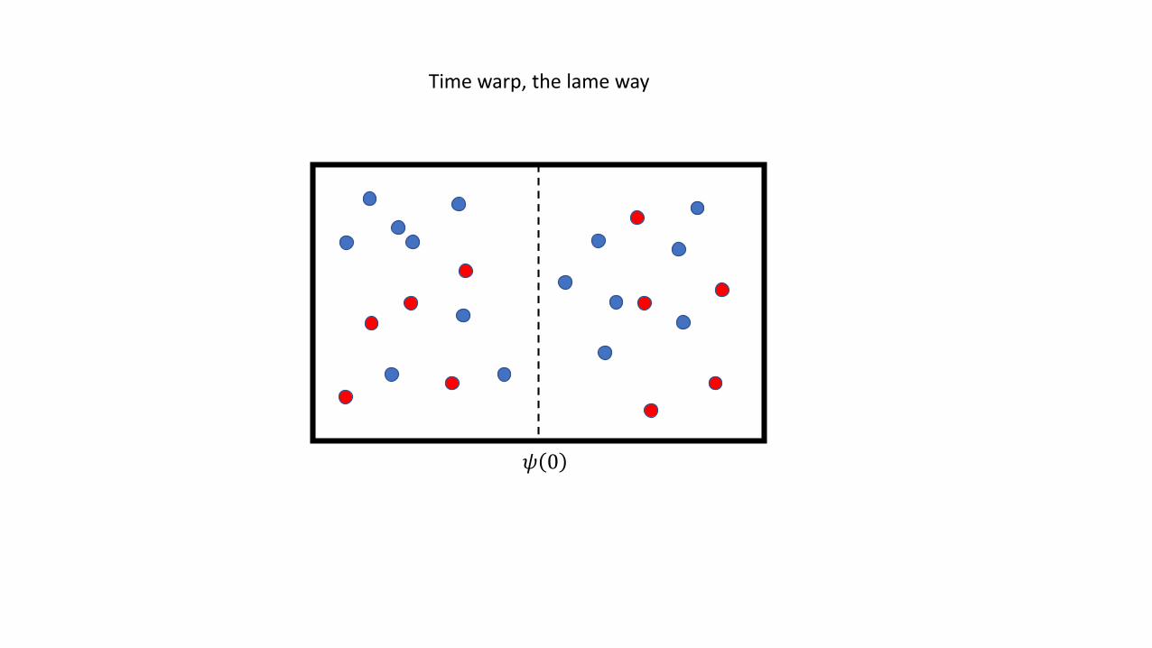
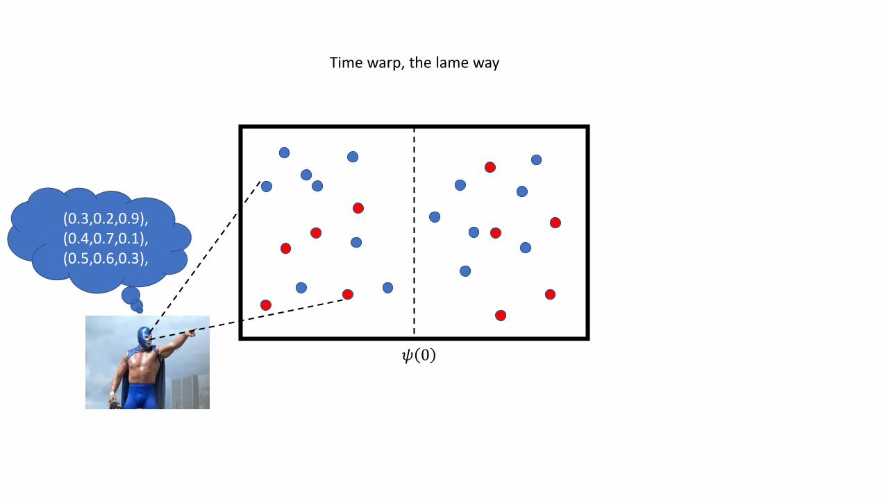
Time warp, the lame way
𝜓 0
𝜓 0
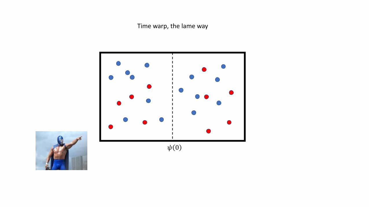
Time warp, the lame way
𝜓 0
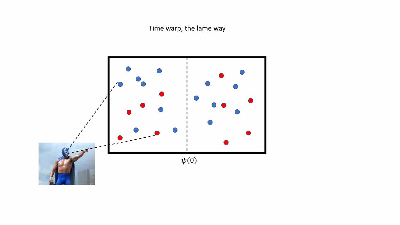
Time warp, the lame way
𝜓 0
(0.3,0.2,0.9),(0.4,0.7,0.1),(0.5,0.6,0.3),
Time warp, the lame way
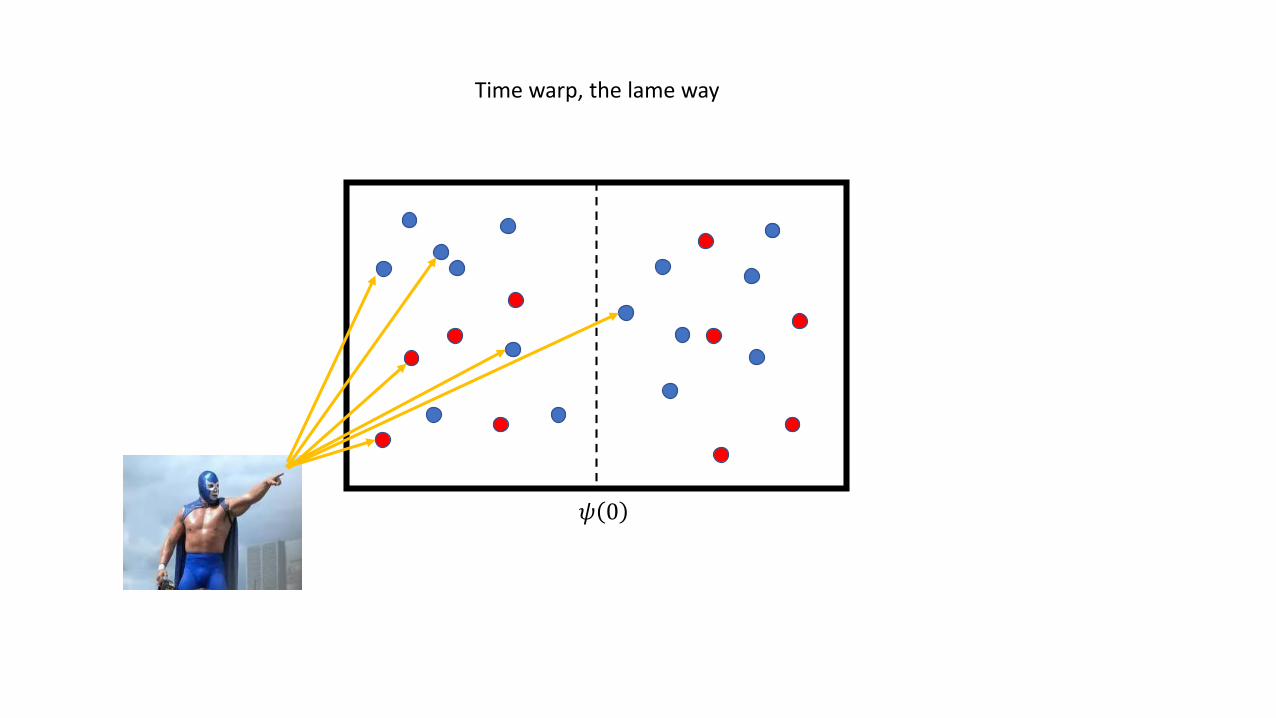
𝜓 0
Time warp, the lame way
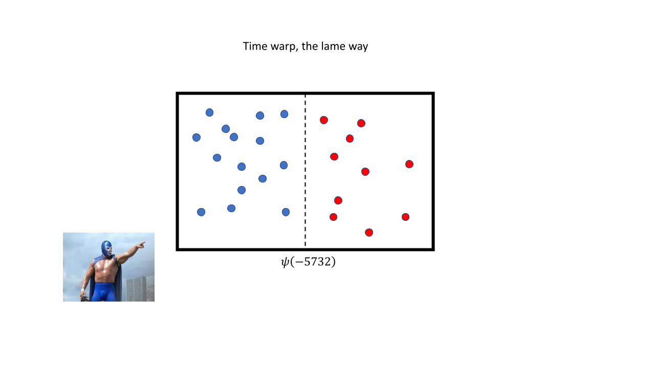
𝜓 −5732
Time warp, the lame way
𝑆
𝑀
|𝜑 =
𝑅
𝑐𝑅 |𝑅
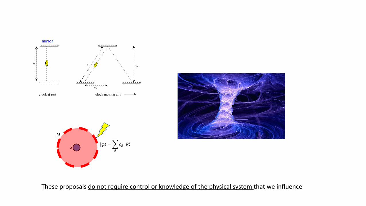
These proposals do not require control or knowledge of the physical system that we influence
𝑆
𝑀
|𝜑 =
𝑅
𝑐𝑅 |𝑅
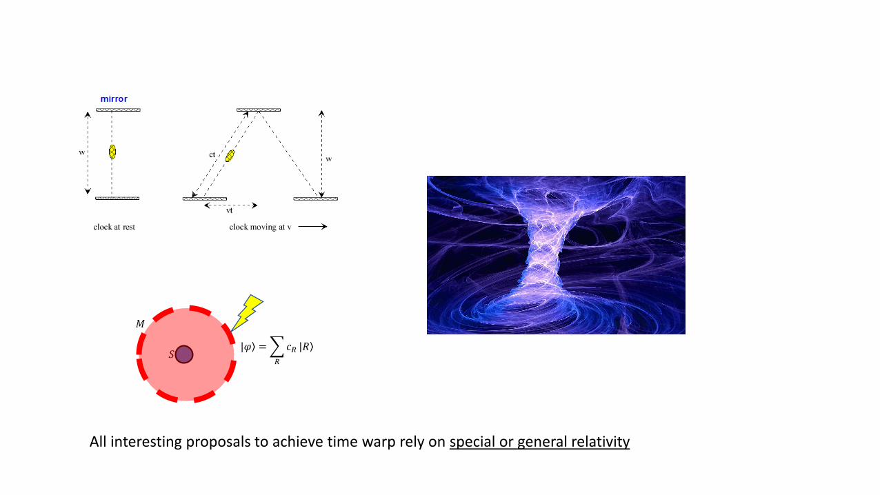
All interesting proposals to achieve time warp rely on special or general relativity

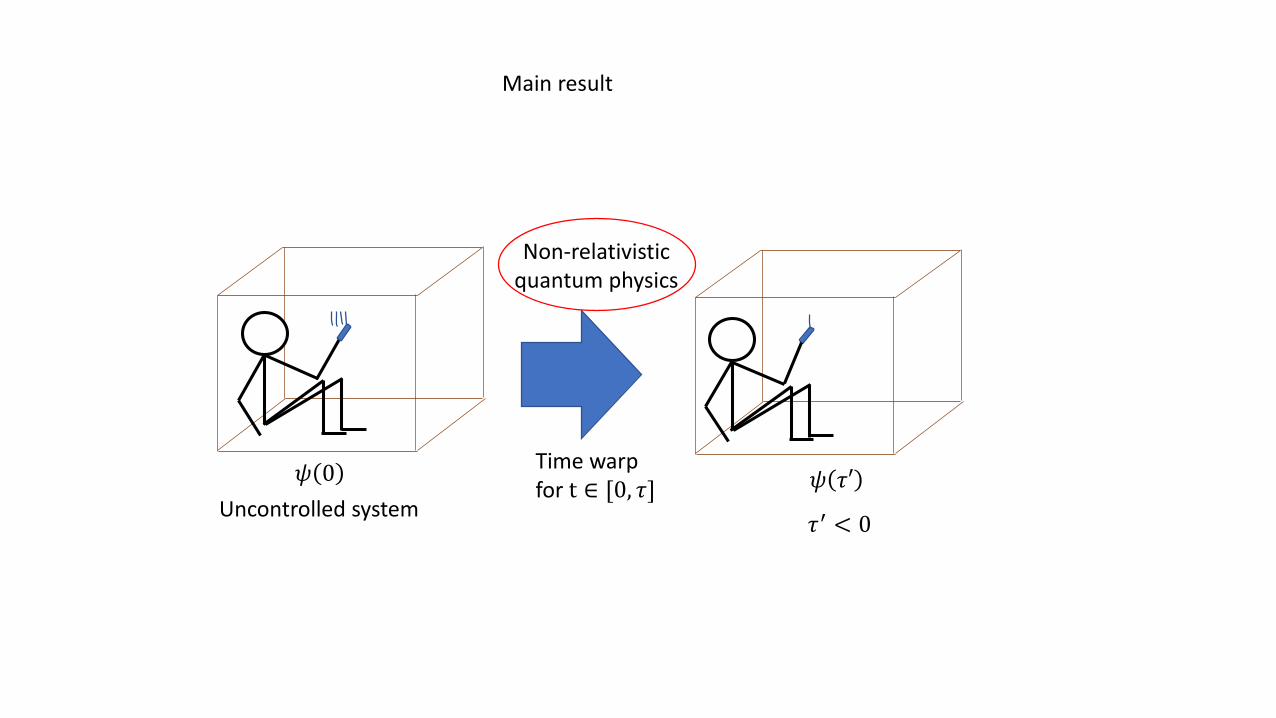
𝜓 𝜏′
𝜏′ < 0
Main result
𝜓 0Time warpfor t ∈ [0, 𝜏]
Uncontrolled system
Non-relativisticquantum physics
𝜓 𝜏′
𝜏′ < 0
Main result
𝜓 0Time warpfor t ∈ [0, 𝜏]
Uncontrolled system
Non-relativisticquantum physics
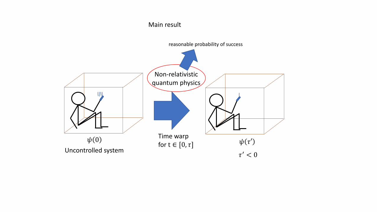
𝜓 𝜏′
𝜏′ < 0
Main result
𝜓 0Time warpfor t ∈ [0, 𝜏]
Uncontrolled system
Non-relativisticquantum physics
reasonable probability of success

Scenario

Goal
𝑆
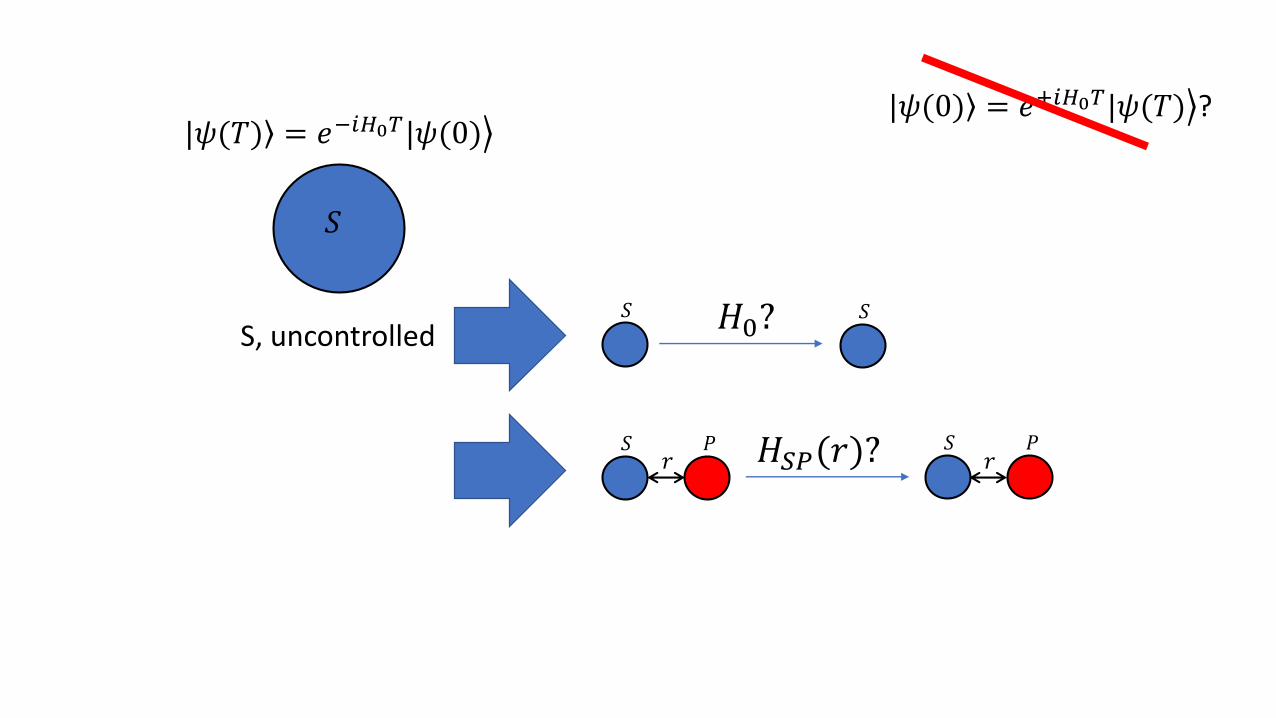
|𝜓(𝑇) = ൿ𝑒−𝑖𝐻0𝑇|𝜓(0)
𝑡 = 𝑇 > 0
𝑆
|𝜓(0)
𝑡 = 𝑇 + Δ
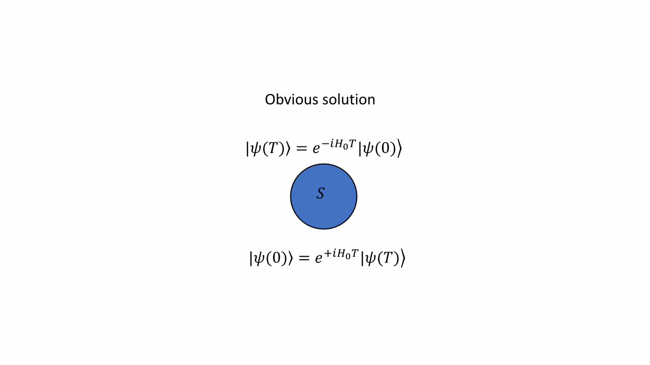
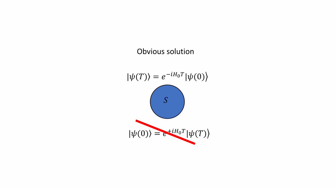
Obvious solution
𝑆
|𝜓(𝑇) = ൿ𝑒−𝑖𝐻0𝑇|𝜓(0)
|𝜓(0) = ൿ𝑒+𝑖𝐻0𝑇|𝜓(𝑇)
𝑆
|𝜓(𝑇) = ൿ𝑒−𝑖𝐻0𝑇|𝜓(0)
|𝜓(0) = ൿ𝑒+𝑖𝐻0𝑇|𝜓(𝑇)
Obvious solution
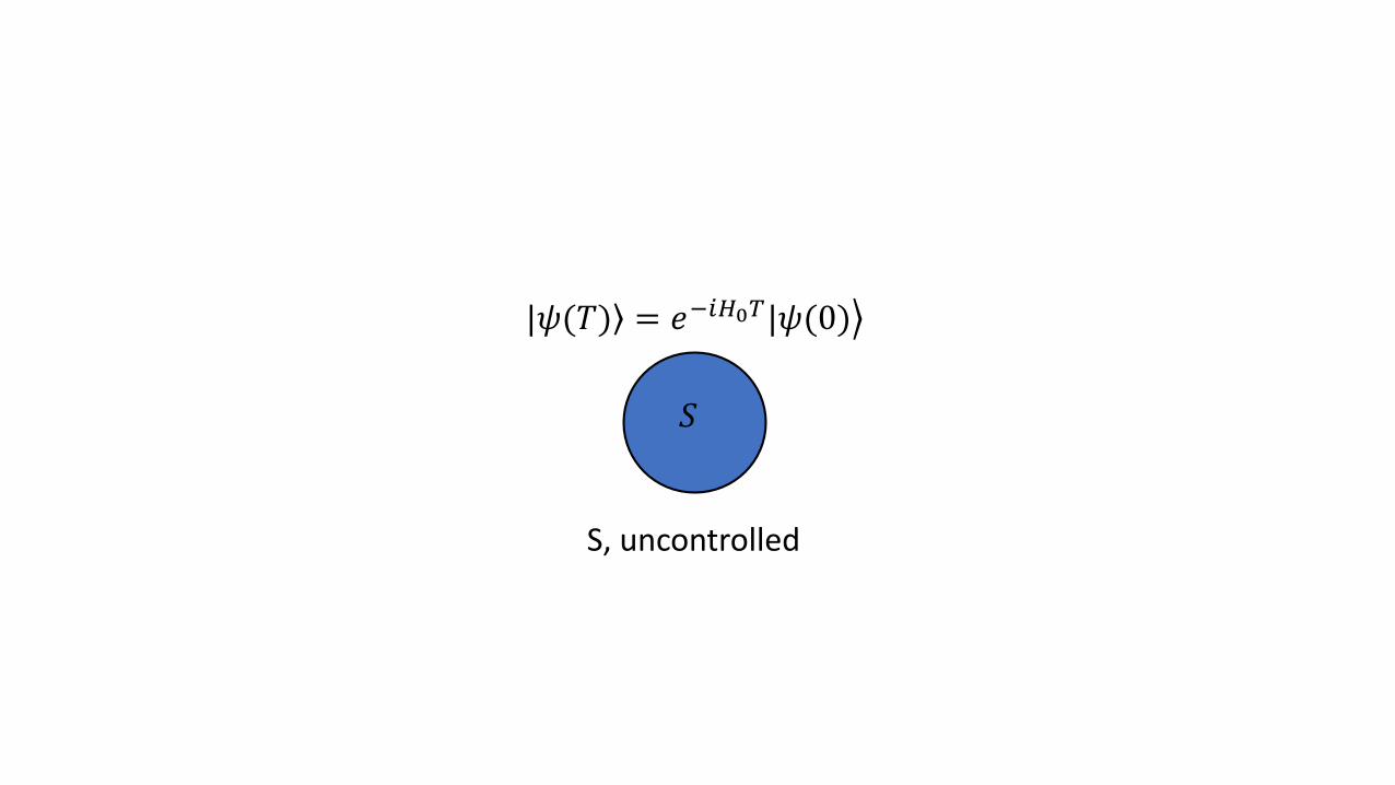
𝑆
|𝜓(𝑇) = ൿ𝑒−𝑖𝐻0𝑇|𝜓(0)
S, uncontrolled
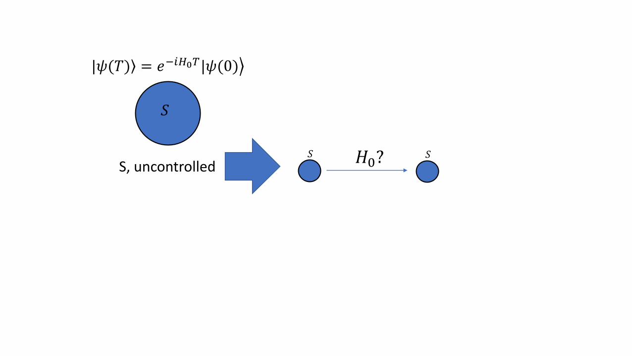
𝑆
|𝜓(𝑇) = ൿ𝑒−𝑖𝐻0𝑇|𝜓(0)
𝐻0?S, uncontrolled𝑆 𝑆
𝑆
|𝜓(𝑇) = ൿ𝑒−𝑖𝐻0𝑇|𝜓(0)
𝐻0?S, uncontrolled
𝑆 𝑃
𝑆 𝑆
𝐻𝑆𝑃(𝑟)?𝑆 𝑃
𝑟 𝑟
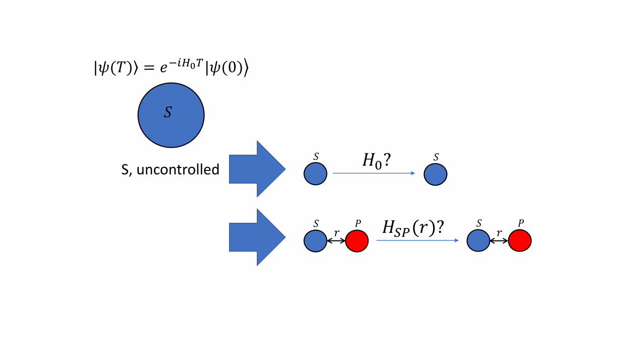
𝑆
|𝜓(𝑇) = ൿ𝑒−𝑖𝐻0𝑇|𝜓(0)
𝐻0?S, uncontrolled
𝑆 𝑃
𝑆 𝑆
𝐻𝑆𝑃(𝑟)?𝑆 𝑃
𝑟 𝑟
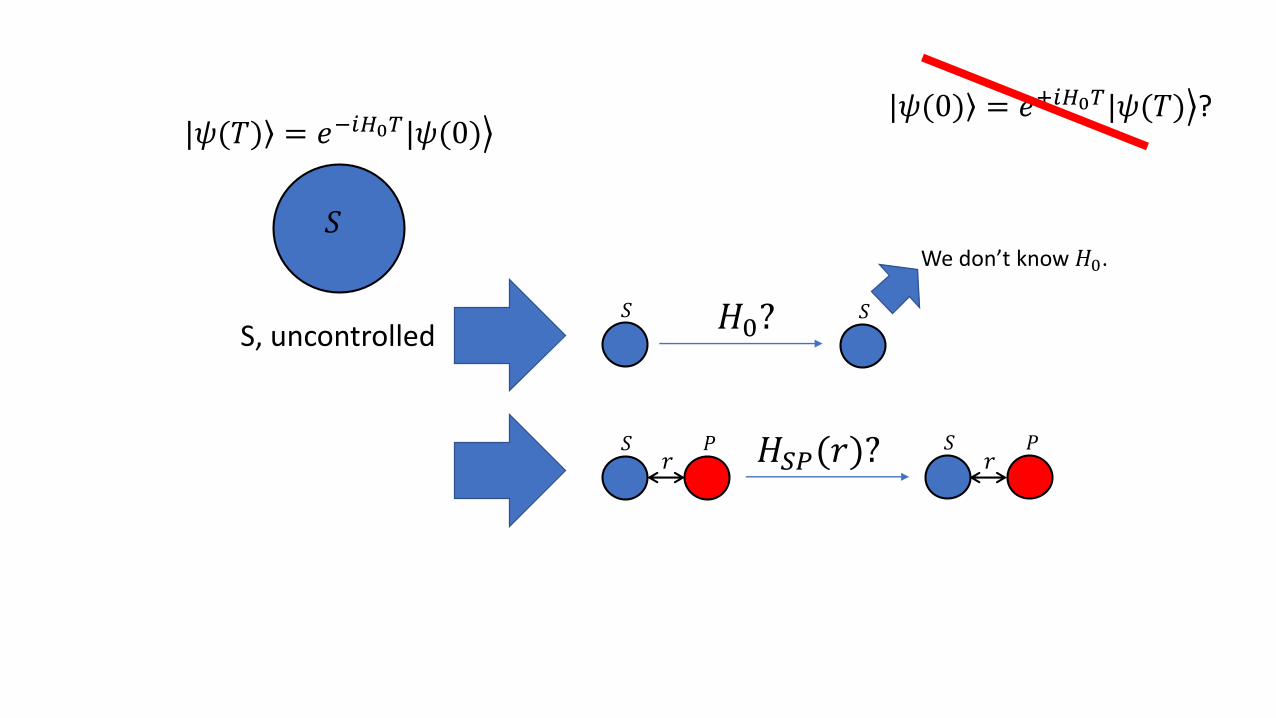
|𝜓(0) = ൿ𝑒+𝑖𝐻0𝑇|𝜓(𝑇) ?
𝑆
|𝜓(𝑇) = ൿ𝑒−𝑖𝐻0𝑇|𝜓(0)
𝐻0?S, uncontrolled
𝑆 𝑃
𝑆 𝑆
𝐻𝑆𝑃(𝑟)?𝑆 𝑃
𝑟 𝑟
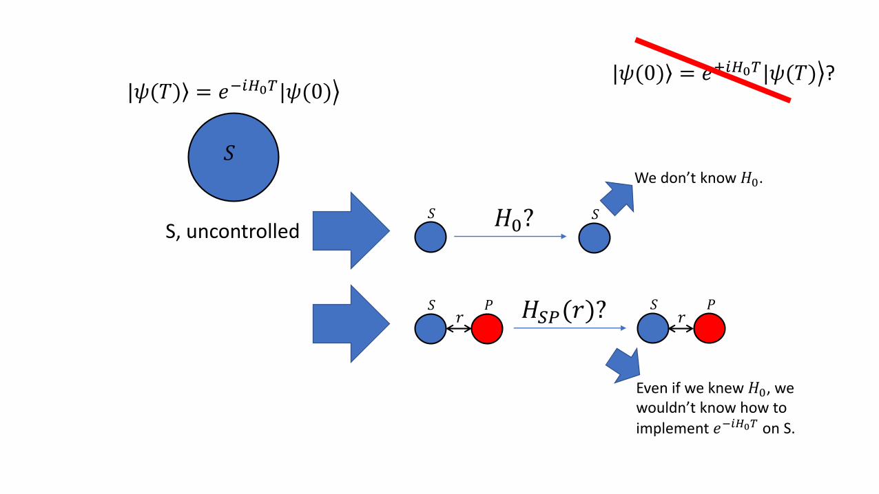
|𝜓(0) = ൿ𝑒+𝑖𝐻0𝑇|𝜓(𝑇) ?
We don’t know 𝐻0.
𝑆
|𝜓(𝑇) = ൿ𝑒−𝑖𝐻0𝑇|𝜓(0)
𝐻0?S, uncontrolled
𝑆 𝑃
𝑆 𝑆
𝐻𝑆𝑃(𝑟)?𝑆 𝑃
𝑟 𝑟
Even if we knew 𝐻0, we wouldn’t know how to
implement 𝑒−𝑖𝐻0𝑇 on S.
We don’t know 𝐻0.
|𝜓(0) = ൿ𝑒+𝑖𝐻0𝑇|𝜓(𝑇) ?
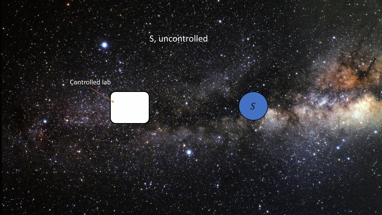
𝑆
Controlled lab
S, uncontrolled
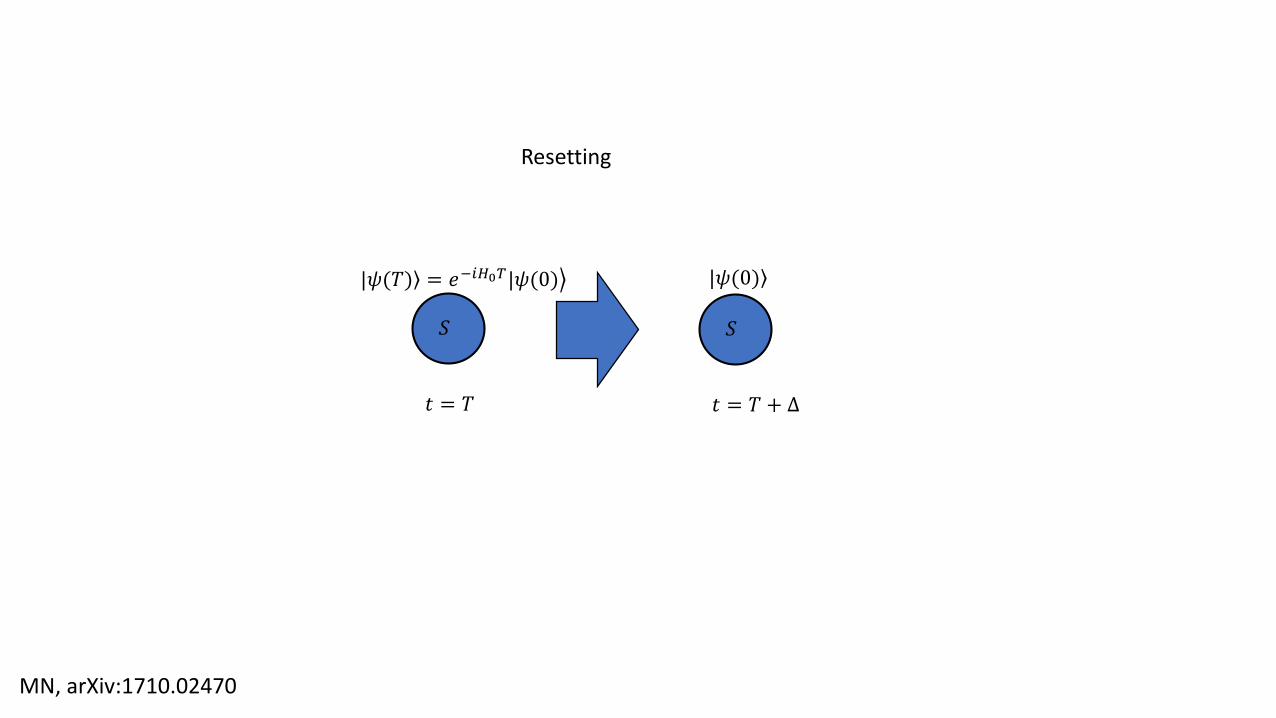
Resetting
𝑆
|𝜓(𝑇) = ൿ𝑒−𝑖𝐻0𝑇|𝜓(0)
𝑡 = 𝑇
𝑆
|𝜓(0)
𝑡 = 𝑇 + Δ
MN, arXiv:1710.02470
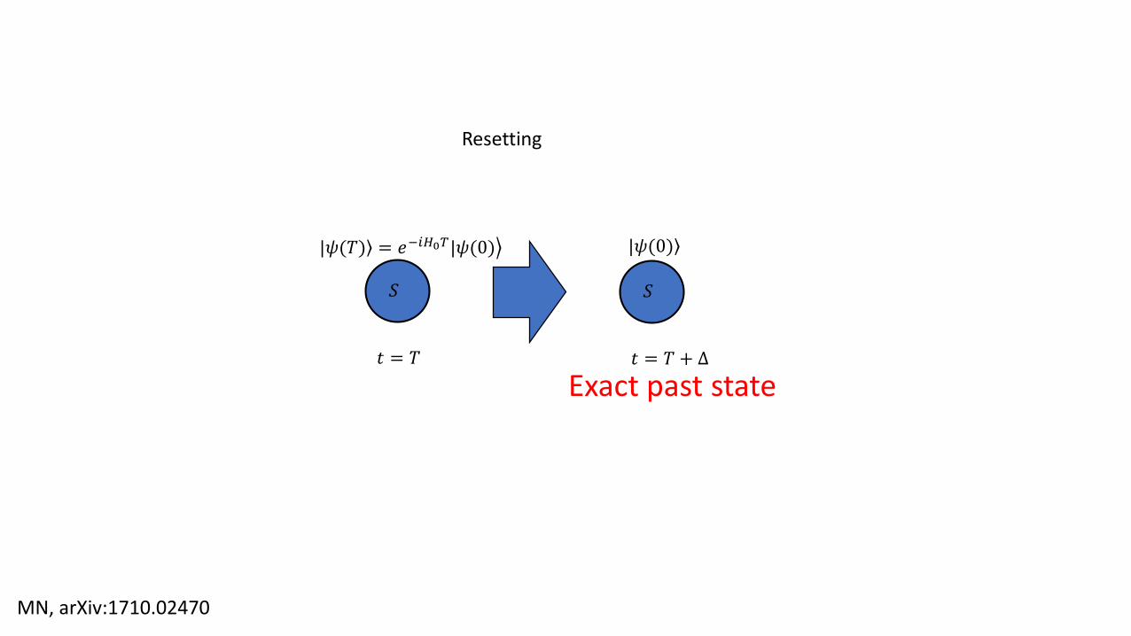
Resetting
𝑆
|𝜓(𝑇) = ൿ𝑒−𝑖𝐻0𝑇|𝜓(0)
𝑡 = 𝑇
𝑆
|𝜓(0)
𝑡 = 𝑇 + Δ
MN, arXiv:1710.02470
Exact past state
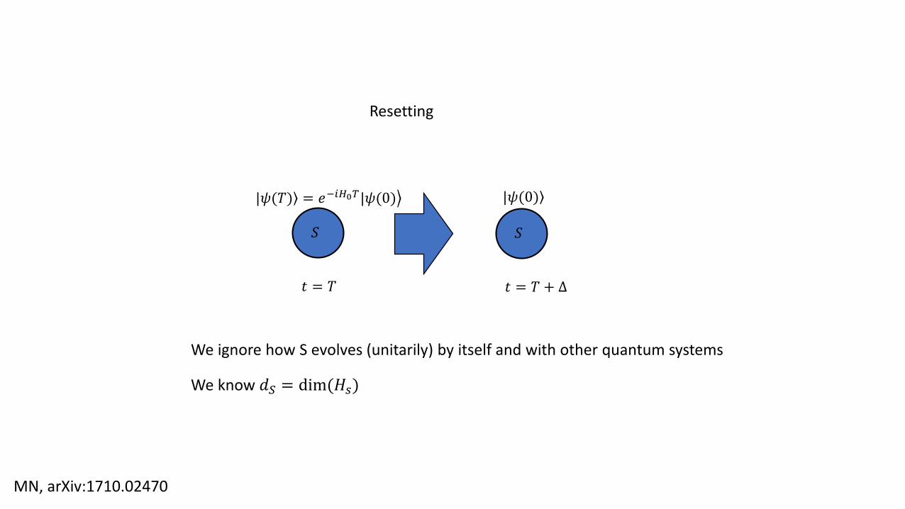
Resetting
𝑆
|𝜓(𝑇) = ൿ𝑒−𝑖𝐻0𝑇|𝜓(0)
𝑡 = 𝑇
𝑆
|𝜓(0)
𝑡 = 𝑇 + Δ
We ignore how S evolves (unitarily) by itself and with other quantum systems
MN, arXiv:1710.02470
We know 𝑑𝑆 = dim(𝐻𝑠)
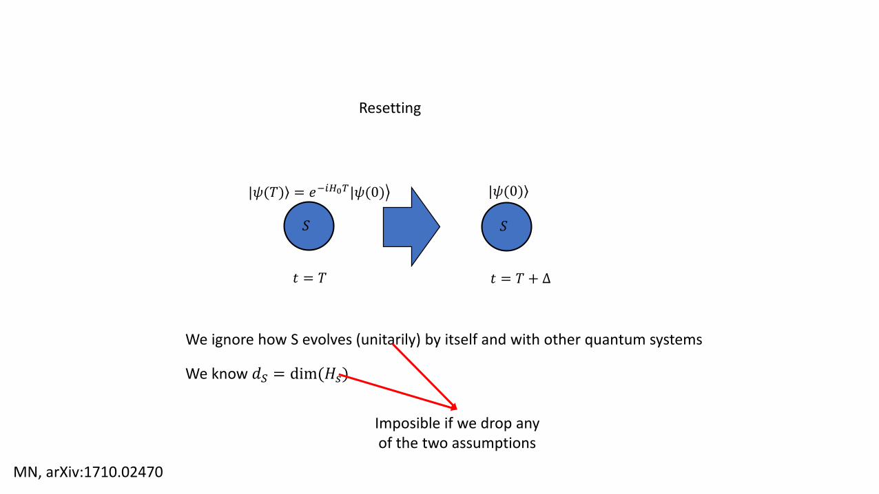
Resetting
𝑆
|𝜓(𝑇) = ൿ𝑒−𝑖𝐻0𝑇|𝜓(0)
𝑡 = 𝑇
𝑆
|𝜓(0)
𝑡 = 𝑇 + Δ
We ignore how S evolves (unitarily) by itself and with other quantum systems
MN, arXiv:1710.02470
We know 𝑑𝑆 = dim(𝐻𝑠)
Imposible if we drop anyof the two assumptions
Sketch of a quantum resetting protocol
𝑆
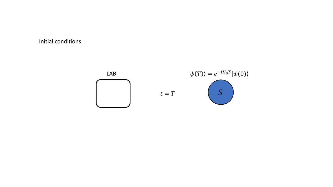
|𝜓(𝑇) = ൿ𝑒−𝑖𝐻0𝑇|𝜓(0)LAB
𝑡 = 𝑇
Initial conditions
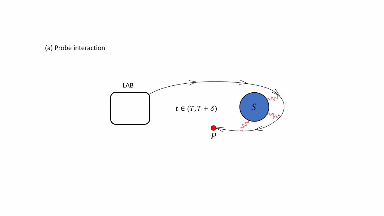
(a) Probe interaction
𝑆
LAB
𝑡 ∈ (𝑇, 𝑇 + 𝛿)
𝑃
𝑆
LAB
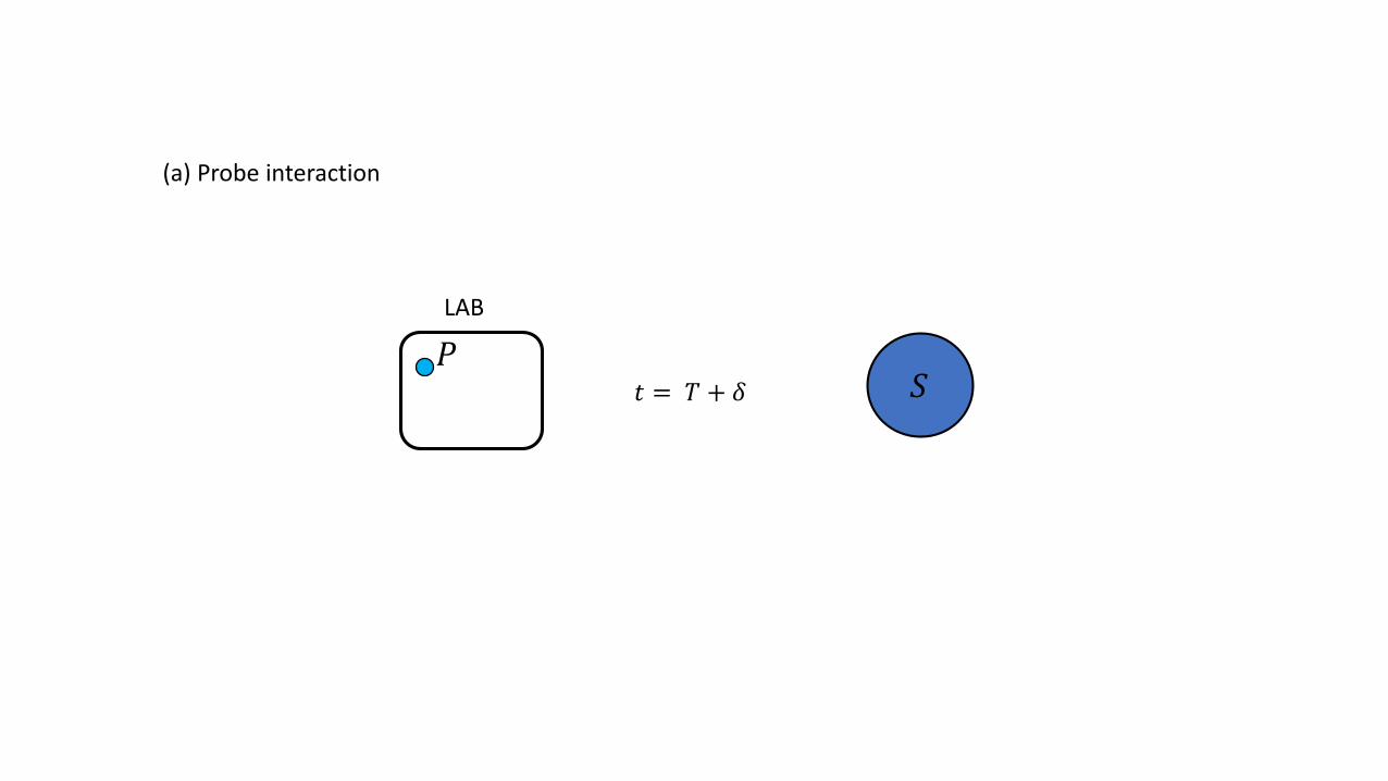
𝑡 = 𝑇 + 𝛿
𝑃
(a) Probe interaction

𝑆
LAB
𝑡 ∈ (𝑇 + 𝛿, 2𝑇 + 𝛿)
𝑃
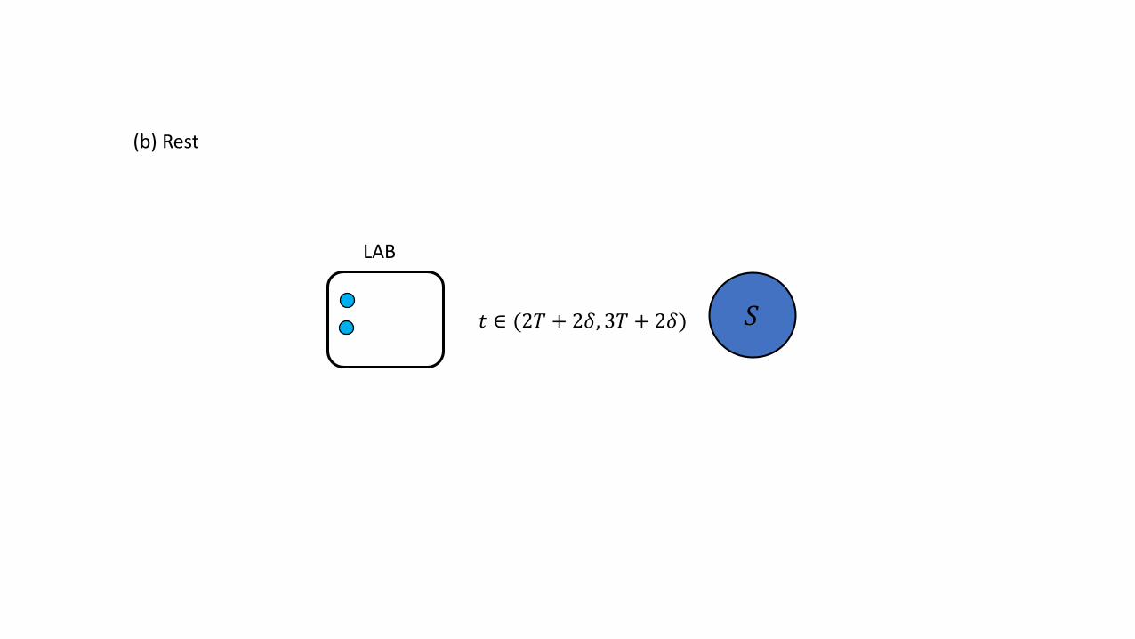
(b) Rest
𝑆
LAB
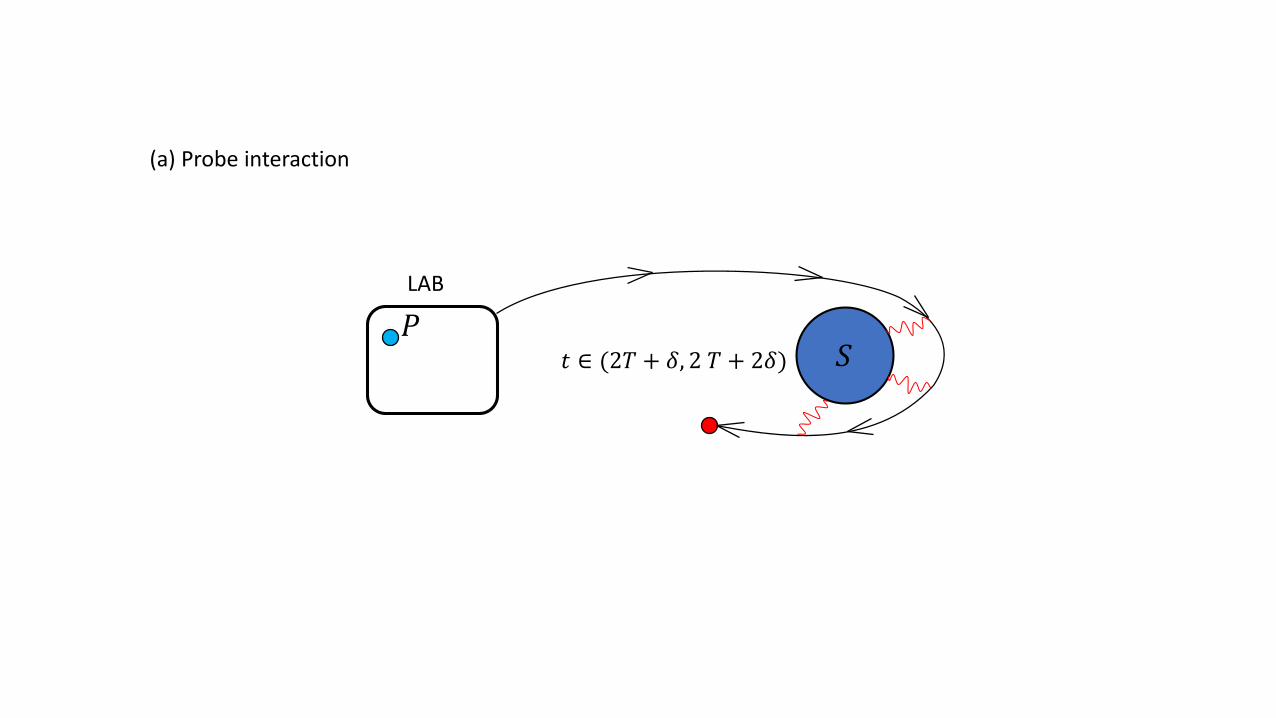
𝑡 ∈ (2𝑇 + 𝛿, 2 𝑇 + 2𝛿)
𝑃
(a) Probe interaction
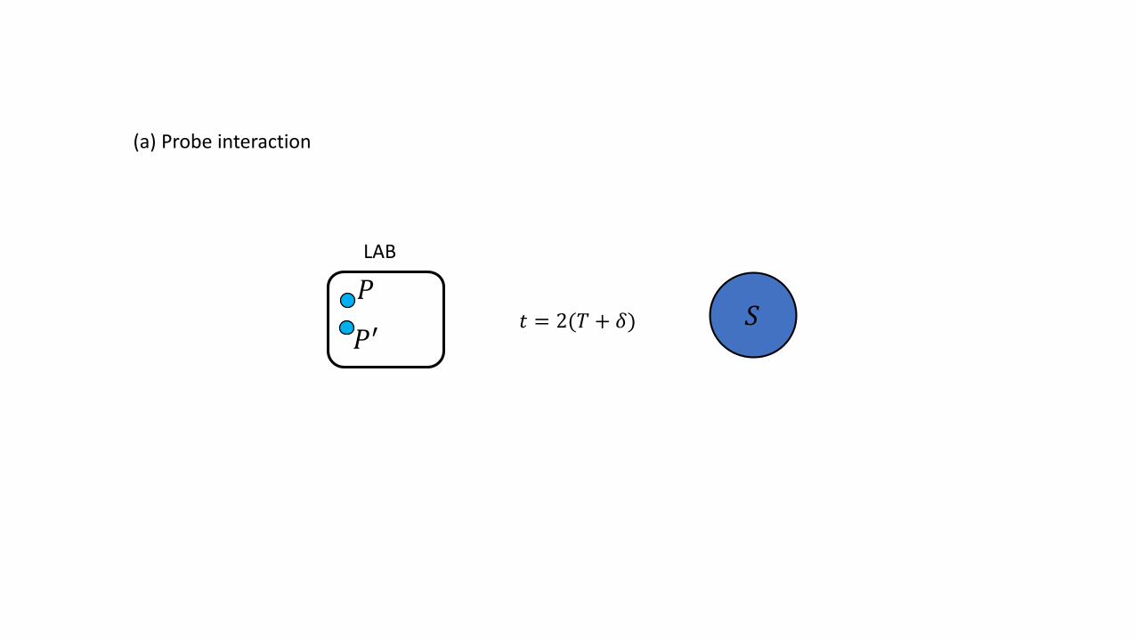
𝑆
LAB
𝑡 = 2(𝑇 + 𝛿)
𝑃
𝑃′
(a) Probe interaction
𝑆
LAB
𝑡 ∈ (2𝑇 + 2𝛿, 3𝑇 + 2𝛿)
(b) Rest

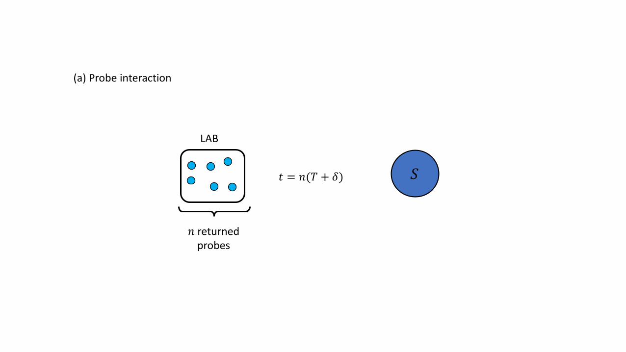
𝑆
LAB
𝑡 = 𝑛(𝑇 + 𝛿)
𝑛 returned probes
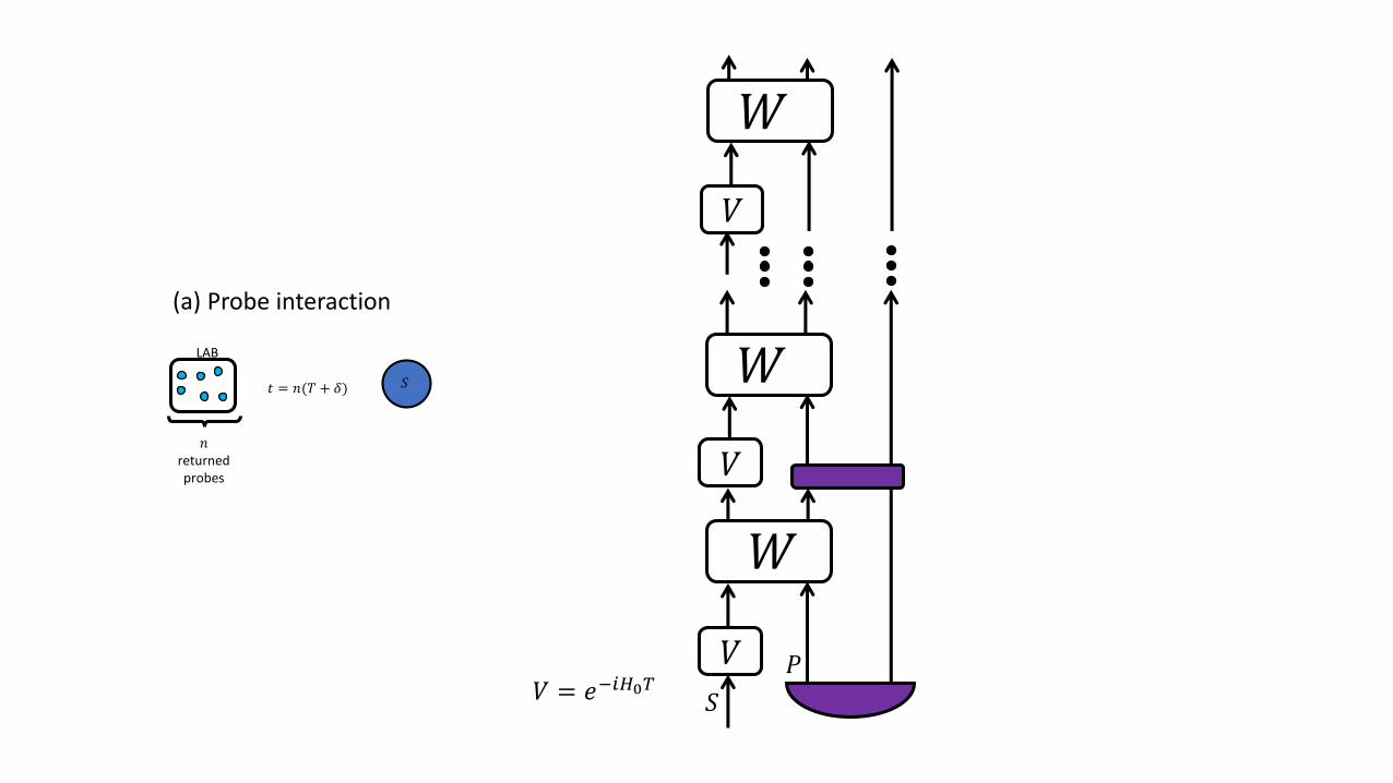
(a) Probe interaction
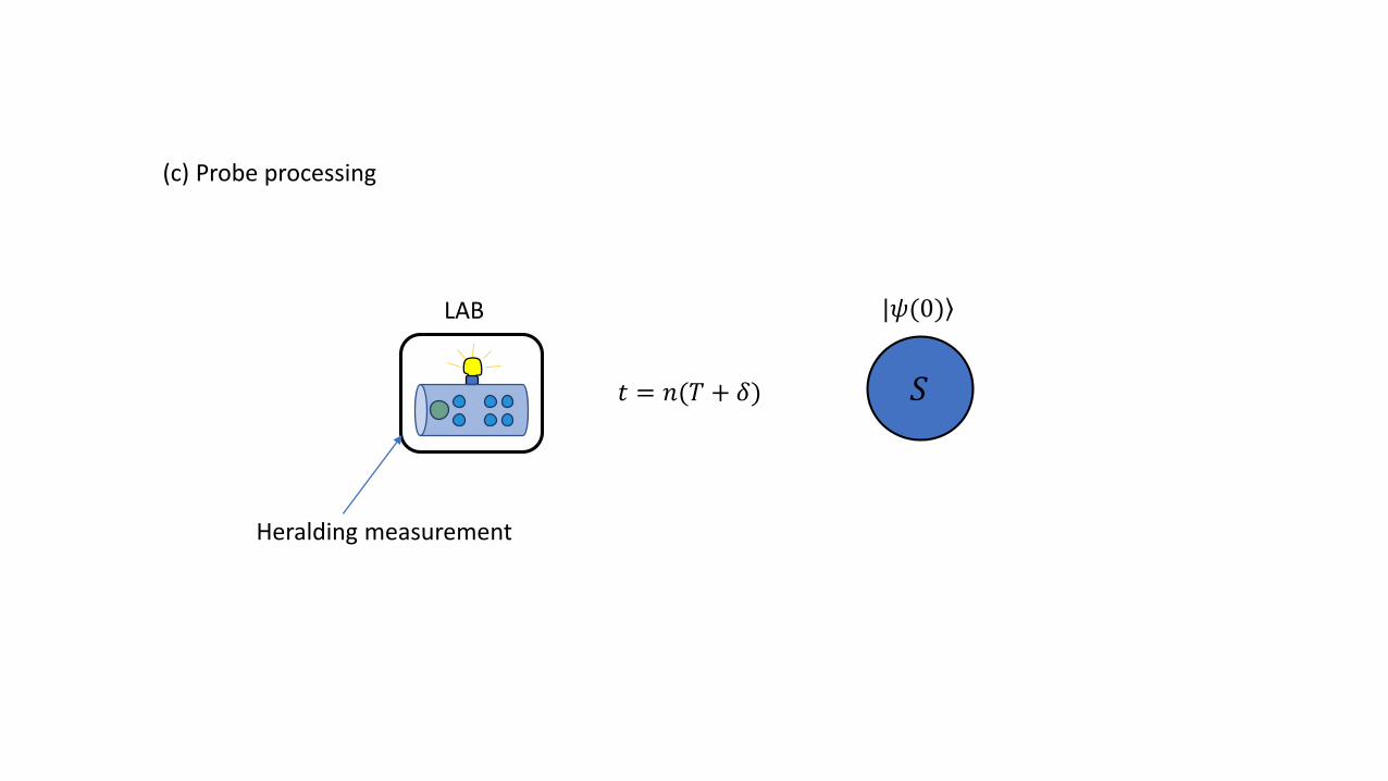
Heralding measurement
𝑆
|𝜓(0)LAB
𝑡 = 𝑛(𝑇 + 𝛿)
(c) Probe processing

In the language of process diagrams
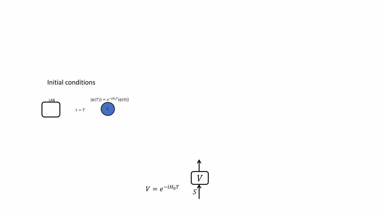
𝑆
|𝜓(𝑇) = ൿ𝑒−𝑖𝐻0𝑇|𝜓(0)LAB
𝑡 = 𝑇
Initial conditions
𝑉 = 𝑒−𝑖𝐻0𝑇 𝑆
𝑉
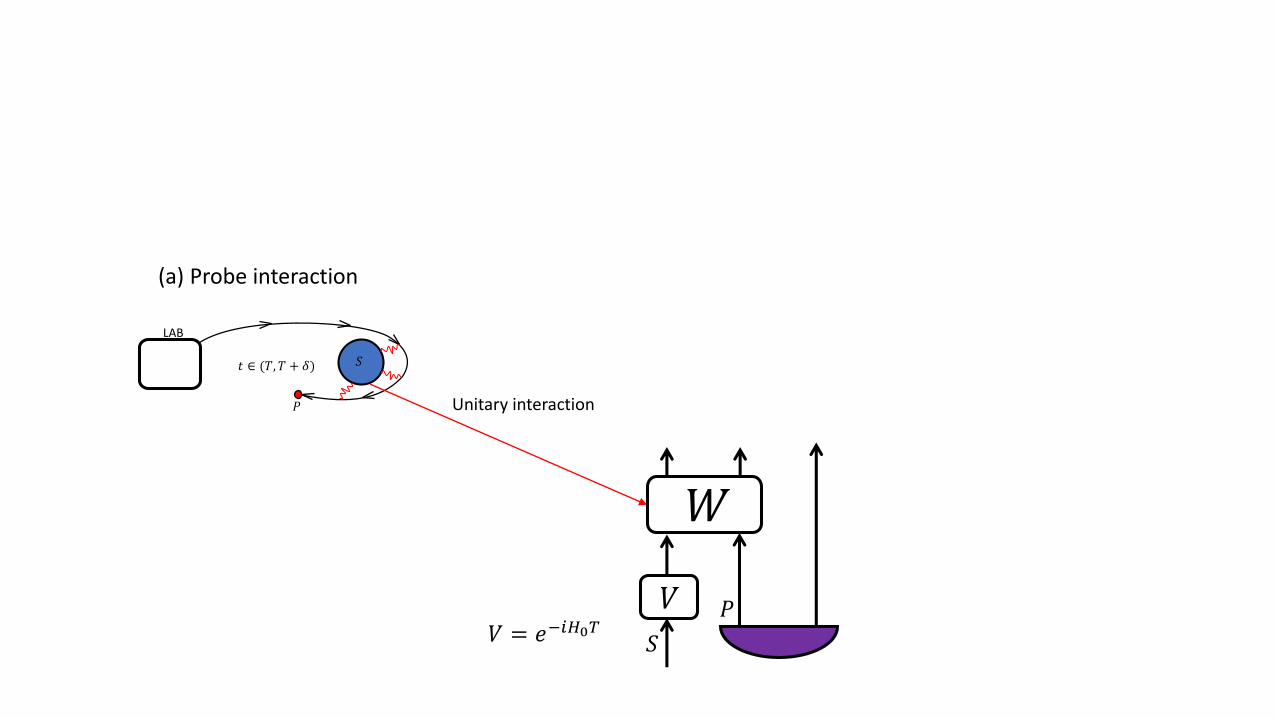
(a) Probe interaction
𝑉 = 𝑒−𝑖𝐻0𝑇
𝑆
LAB
𝑡 ∈ (𝑇, 𝑇 + 𝛿)
𝑃 Unitary interaction
𝑆
𝑊
𝑉 𝑃

(b) Rest
𝑉 = 𝑒−𝑖𝐻0𝑇
𝑆
LAB
𝑡 ∈ (𝑇 + 𝛿, 2𝑇 + 𝛿)𝑃
𝑆
𝑊
𝑉 𝑃
𝑉

𝑉 = 𝑒−𝑖𝐻0𝑇 𝑆
𝑊
𝑉 𝑃
𝑉
(a) Probe interaction
𝑊
𝑉
𝑊
𝑆
LAB
𝑡 = 𝑛(𝑇 + 𝛿)
𝑛returned probes
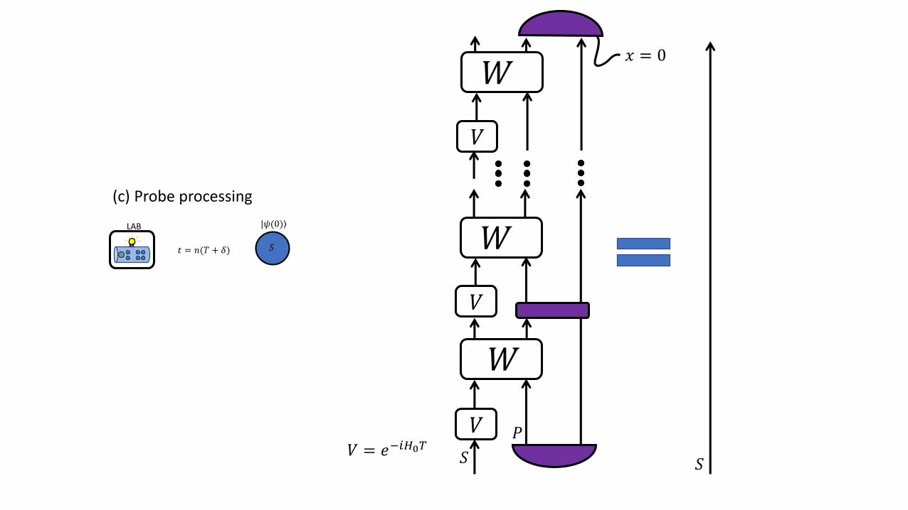
𝑉 = 𝑒−𝑖𝐻0𝑇
(c) Probe processing
𝑆
|𝜓(0)LAB
𝑡 = 𝑛(𝑇 + 𝛿)
𝑆
𝑊
𝑉 𝑃
𝑉
𝑊
𝑉
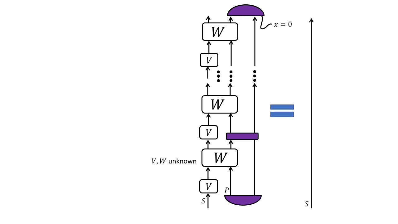
𝑊
𝑆
𝑥 = 0
𝑆
𝑊
𝑉 𝑃
𝑉
𝑊
𝑉
𝑊
𝑆
𝑉,𝑊 unknown
𝑥 = 0

𝑆
𝑊
𝑉 𝑃
𝑉
𝑊
𝑉
𝑊
𝑆
𝑆
𝑊
𝑉 𝑃 𝑆
𝑈𝑃
𝑉,𝑊 unknown
𝑥 = 0
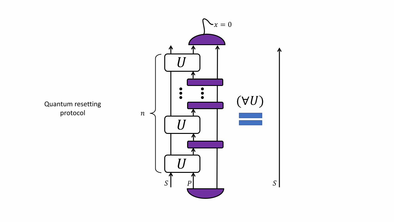
(∀𝑈)
𝑆𝑆
𝑈
𝑈
𝑈𝑃
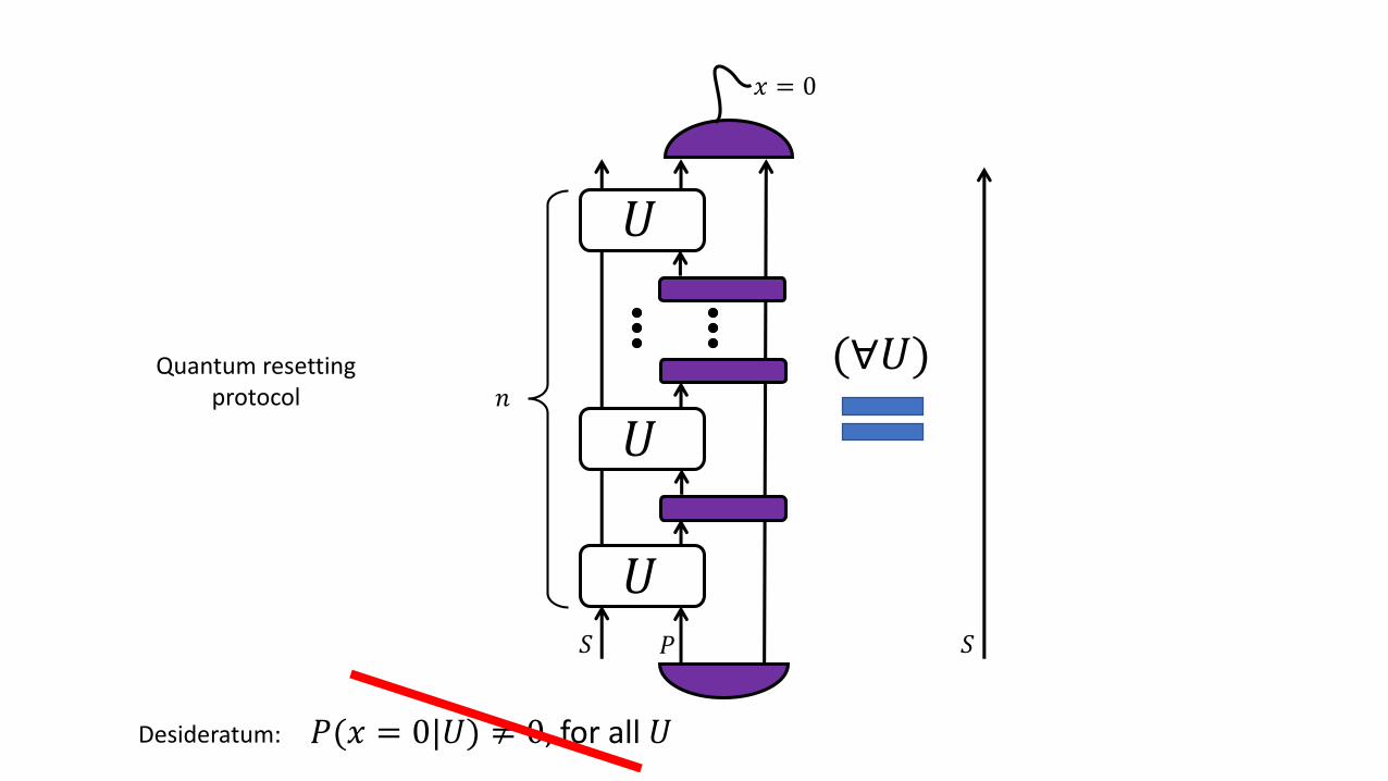
𝑛Quantum resetting
protocol
𝑥 = 0
(∀𝑈)
𝑆𝑆
𝑈
𝑈
𝑈𝑃
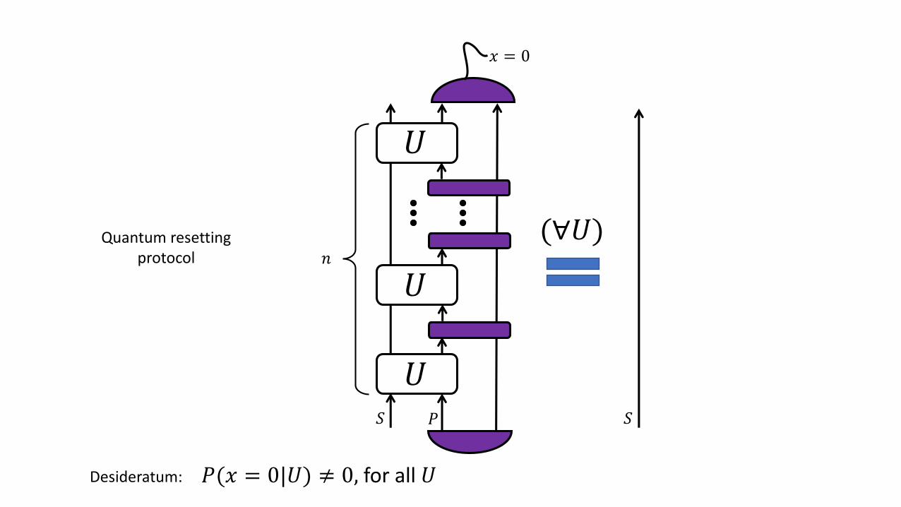
𝑛Quantum resetting
protocol
𝑥 = 0
Desideratum: 𝑃(𝑥 = 0|𝑈) ≠ 0, for all 𝑈
𝑆
𝑈
𝑈
𝑈𝑃
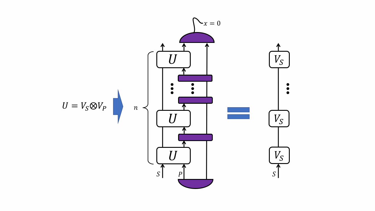
𝑛𝑈 = 𝑉𝑆⨂𝑉𝑃
𝑆
𝑉𝑆
𝑉𝑆
𝑉𝑆
𝑥 = 0
𝑈 = 𝑉𝑆⨂𝑉𝑃 Resetting protocol will fail with probability 1
(∀𝑈)
𝑆𝑆
𝑈
𝑈
𝑈𝑃
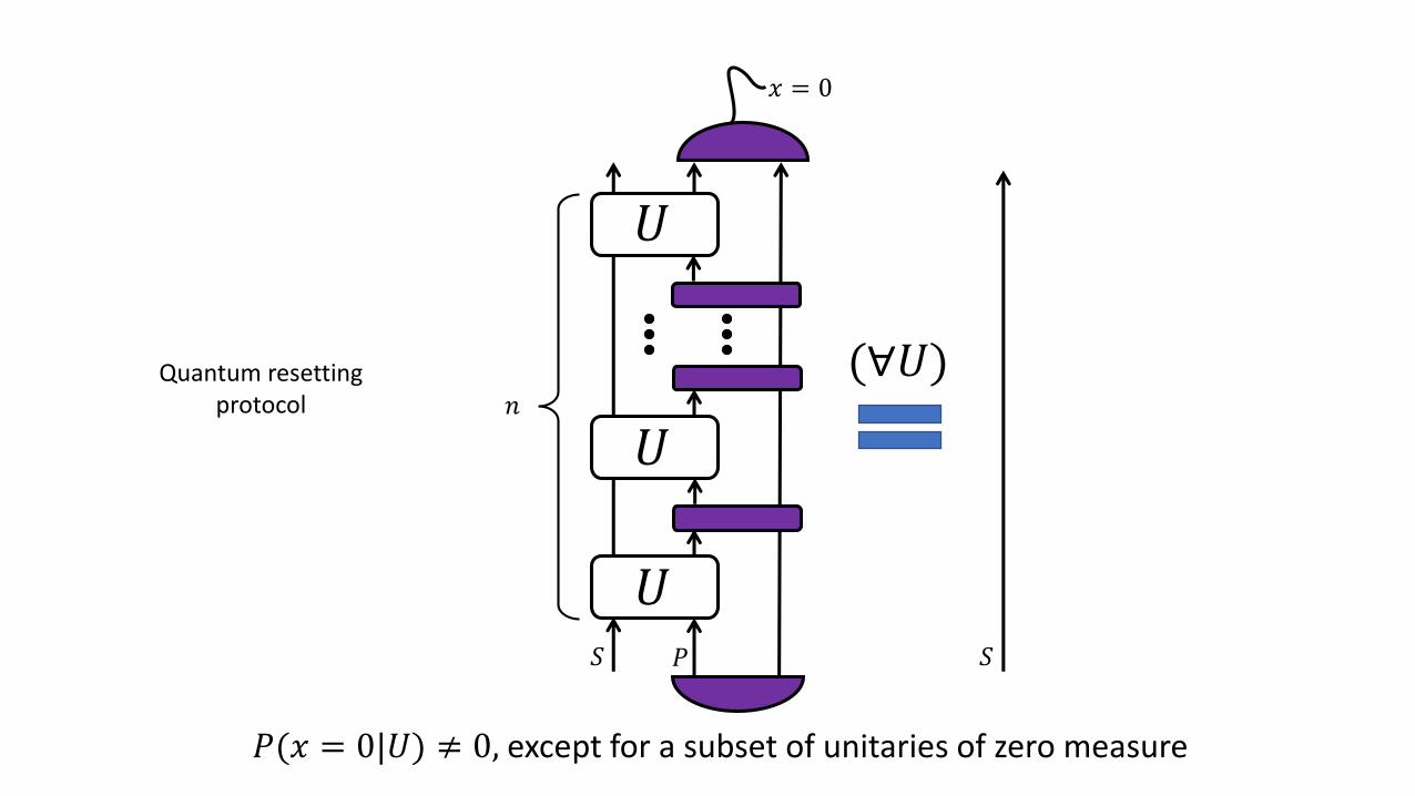
𝑛Quantum resetting
protocol
𝑥 = 0
Desideratum: 𝑃(𝑥 = 0|𝑈) ≠ 0, for all 𝑈
𝑆
𝑈
𝑈
𝑈𝑃
𝑥 = 0
(∀𝑈)
𝑆
𝑛Quantum resetting
protocol
𝑃(𝑥 = 0|𝑈) ≠ 0, except for a subset of unitaries of zero measure

Do quantum resetting protocols exist?
𝑆
LAB
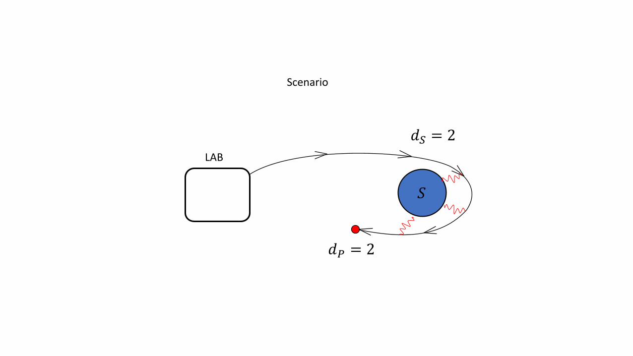
Scenario
𝑑𝑆 = 2
𝑑𝑃 = 2
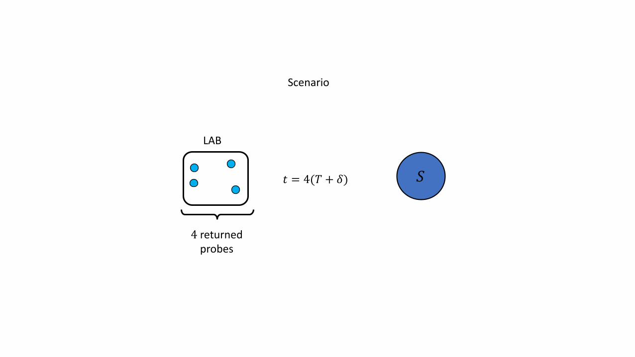
𝑆
LAB
𝑡 = 4(𝑇 + 𝛿)
4 returned probes
Scenario
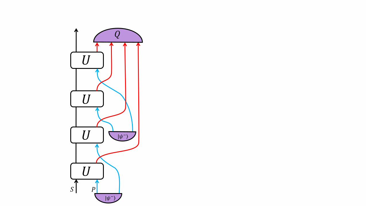
𝑆
𝑈
𝑈
𝑈
𝑈𝑃
𝑄
|𝜓−
|𝜓−
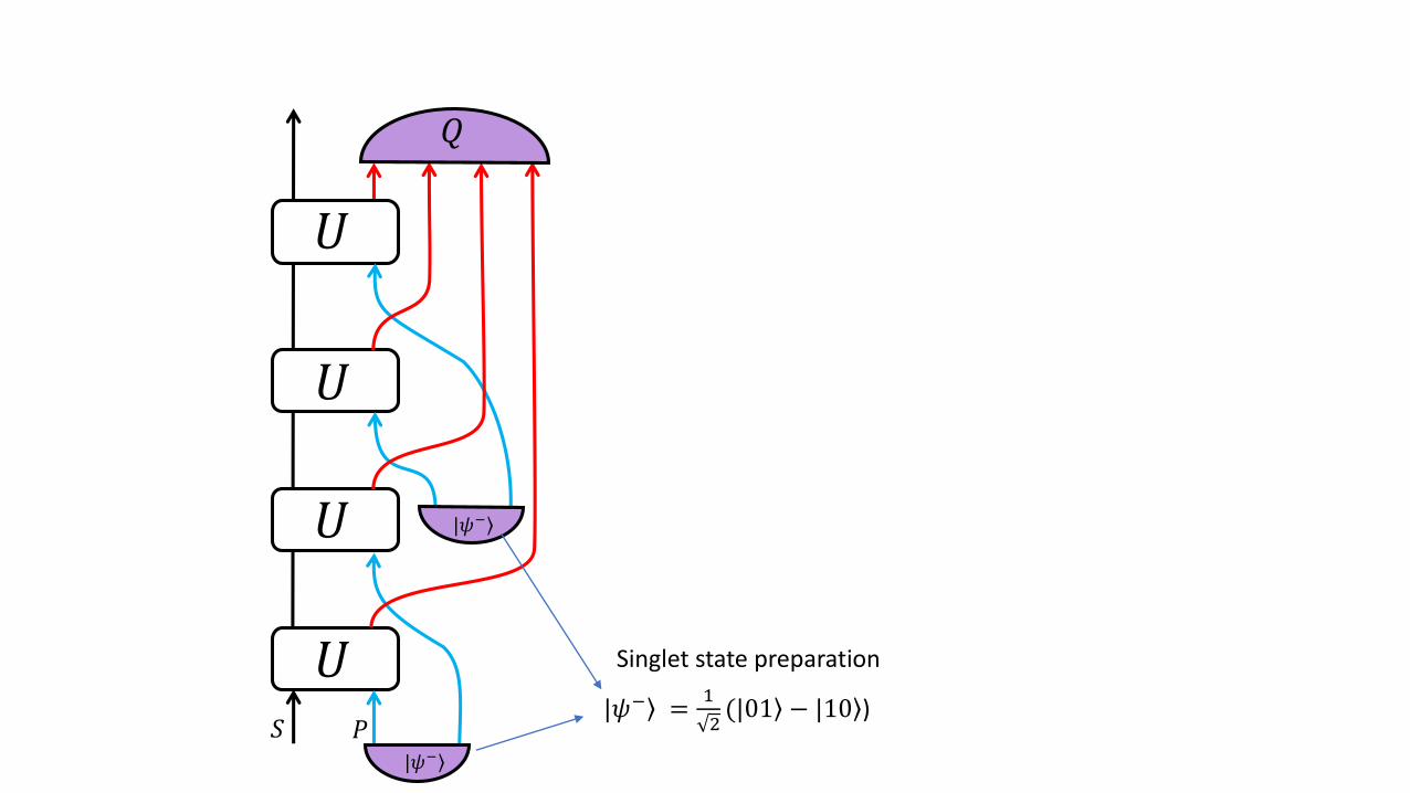
𝑆
𝑈
𝑈
𝑈
𝑈𝑃
𝑄
|𝜓−
|𝜓−
Singlet state preparation
|𝜓− =1
2( |01 − |10 )
𝑆
𝑈
𝑈
𝑈
𝑈𝑃
𝑄
|𝜓−
|𝜓−
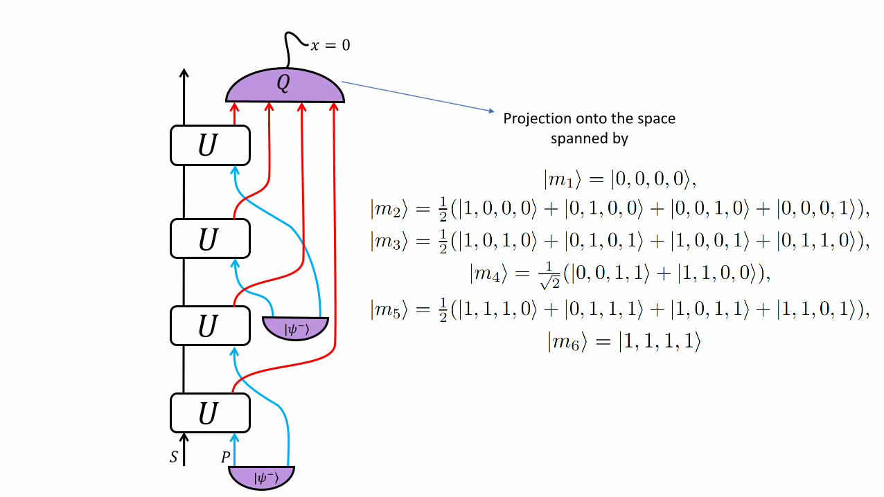
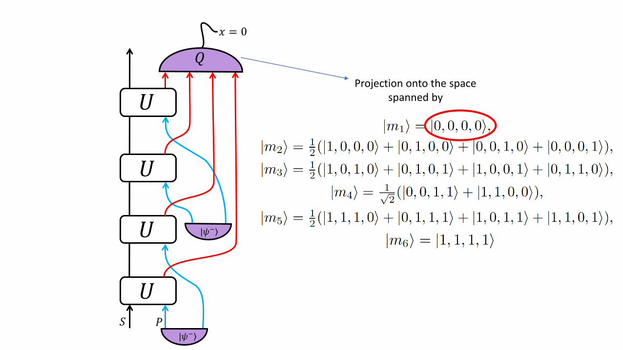
Projection onto the spacespanned by
𝑥 = 0

Why does this work?
𝑆
𝑈
𝑈
𝑈
𝑈𝑃
𝑄
|𝜓−
|𝜓−
Projection onto the spacespanned by
𝑥 = 0
𝑆
𝑈
𝑈
𝑈
𝑈𝑃
|𝜓−
|𝜓−
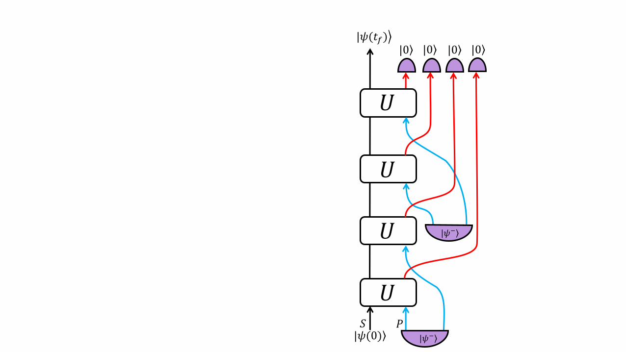
|0 |0 |0 |0ൿ|𝜓(𝑡𝑓)
|𝜓(0)
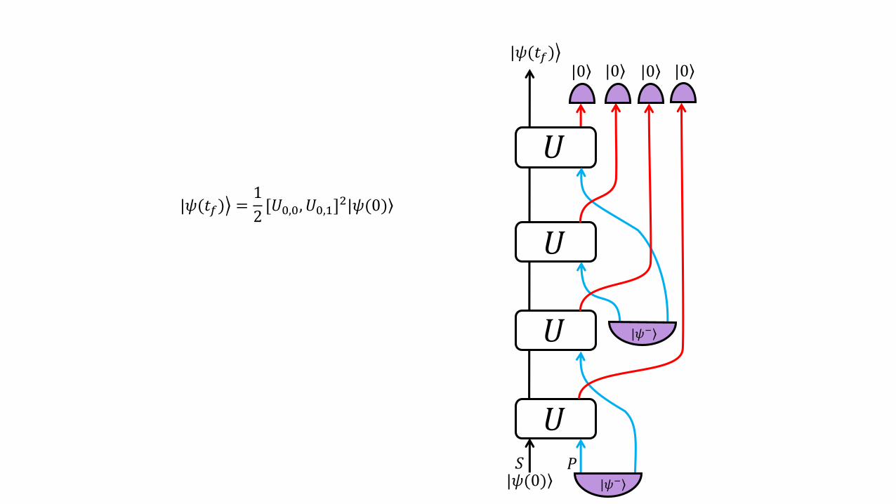
𝑆
𝑈
𝑈
𝑈
𝑈𝑃
|𝜓−
|𝜓−
|0 |0 |0 |0
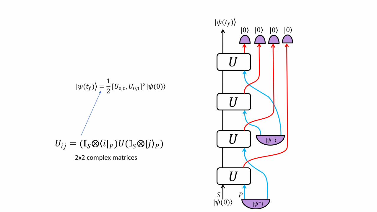
ൿ|𝜓(𝑡𝑓) =1
2[𝑈0,0, 𝑈0,1]
2 |𝜓(0)
ൿ|𝜓(𝑡𝑓)
|𝜓(0)
𝑈𝑖𝑗 = (𝕀𝑆⨂ۦ𝑖|𝑃)𝑈(𝕀𝑆⨂| 𝑗 𝑃)
2x2 complex matrices
𝐴, 𝐵, 2 × 2 matrices
𝐴, 𝐵 =
𝑖=0,1,2,3
𝑐𝑖𝜎𝑖
𝜎𝑖, Pauli matrices
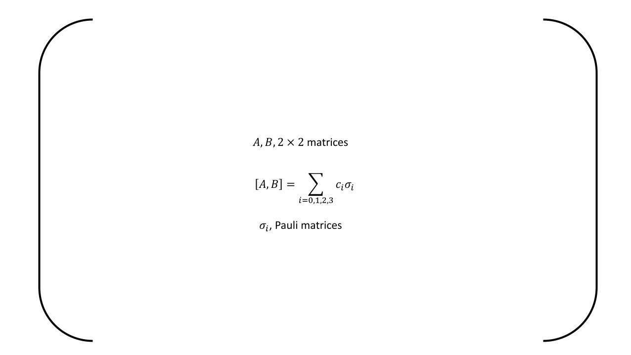
𝐴, 𝐵, 2 × 2 matrices
𝐴, 𝐵 =
𝑖=0,1,2,3
𝑐𝑖𝜎𝑖
𝜎𝑖, Pauli matrices
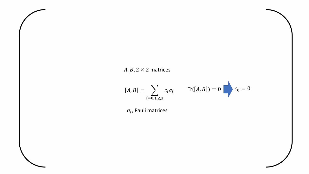
𝐴, 𝐵, 2 × 2 matrices
𝑐0 = 0Tr( 𝐴, 𝐵 ) = 0
𝐴, 𝐵 =
𝑖=1,2,3
𝑐𝑖𝜎𝑖
𝜎𝑖, Pauli matrices
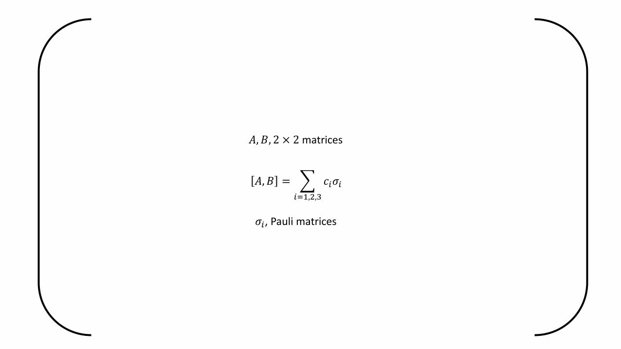
𝐴, 𝐵, 2 × 2 matrices
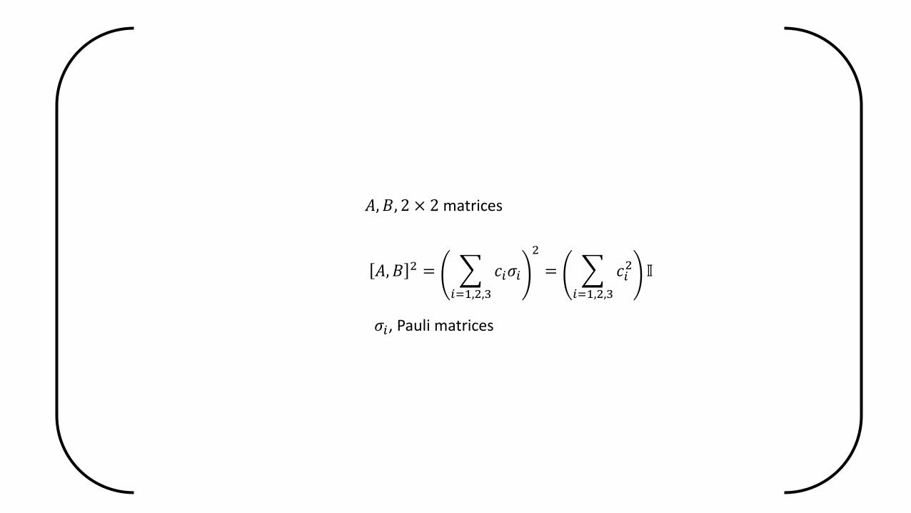
𝐴, 𝐵 2 =
𝑖=1,2,3
𝑐𝑖𝜎𝑖
2
=
𝑖=1,2,3
𝑐𝑖2 𝕀
𝜎𝑖, Pauli matrices
𝐴, 𝐵, 2 × 2 matrices
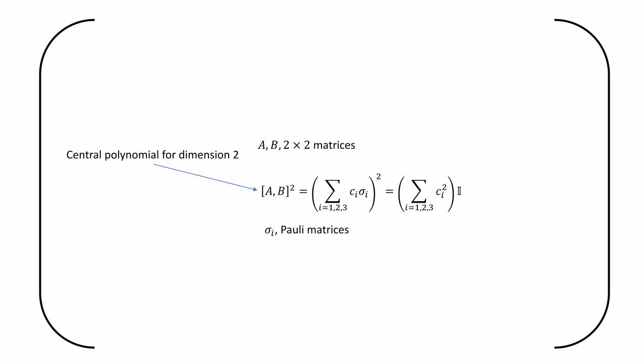
𝐴, 𝐵 2 =
𝑖=1,2,3
𝑐𝑖𝜎𝑖
2
=
𝑖=1,2,3
𝑐𝑖2 𝕀
𝜎𝑖, Pauli matrices
𝐴, 𝐵, 2 × 2 matricesCentral polynomial for dimension 2
𝑆
𝑈
𝑈
𝑈
𝑈𝑃
|𝜓−
|𝜓−
|0 |0 |0 |0
ൿ|𝜓(𝑡𝑓) =1
2[𝑈0,0, 𝑈0,1]
2 |𝜓(0)
ൿ|𝜓(𝑡𝑓)
|𝜓(0)
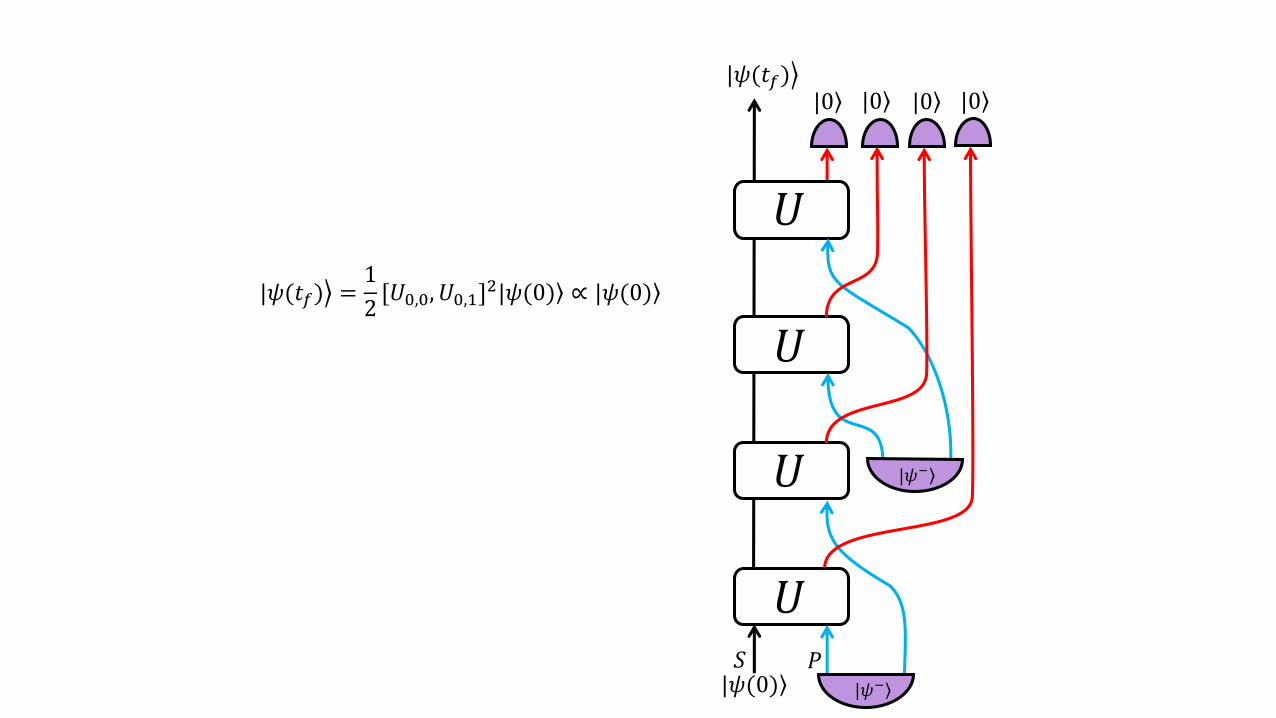
𝑆
𝑈
𝑈
𝑈
𝑈𝑃
|𝜓−
|𝜓−
|0 |0 |0 |0
ൿ|𝜓(𝑡𝑓) =1
2[𝑈0,0, 𝑈0,1]
2 |𝜓(0) ∝ |𝜓(0)
ൿ|𝜓(𝑡𝑓)
|𝜓(0)
𝑆
𝑈
𝑈
𝑈
𝑈𝑃
|𝜓−
|𝜓−
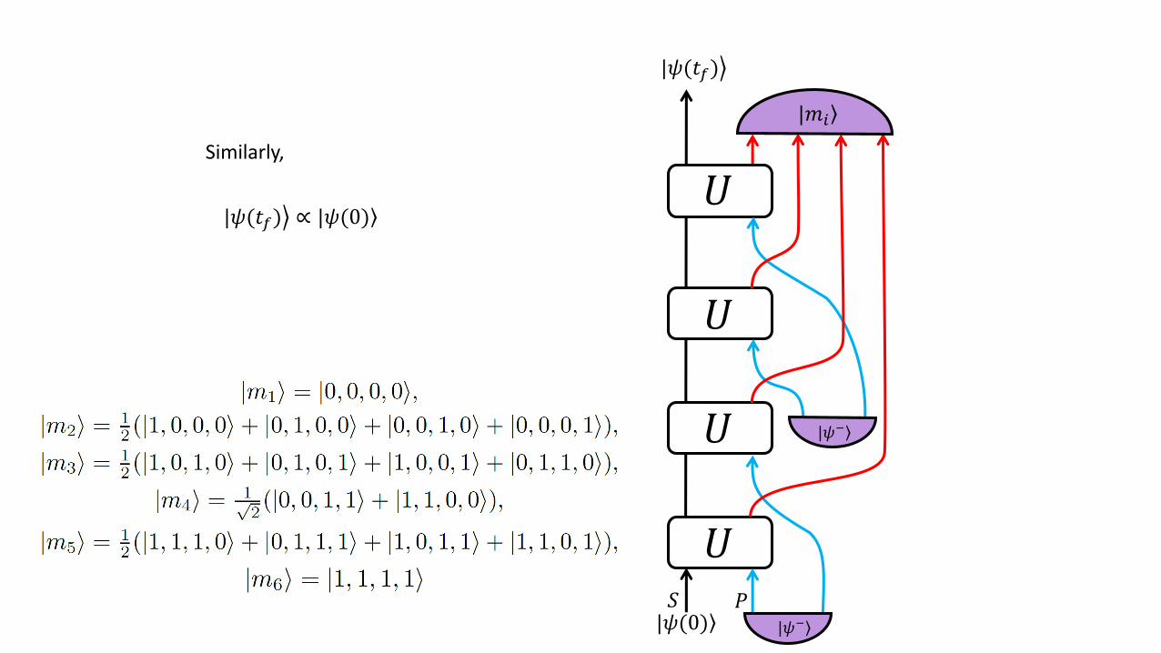
ൿ|𝜓(𝑡𝑓) ∝ |𝜓(0)
ൿ|𝜓(𝑡𝑓)
|𝜓(0)
Similarly,
|𝑚𝑖
𝑆
𝑈
𝑈
𝑈
𝑈𝑃
𝑄
|𝜓−
|𝜓−
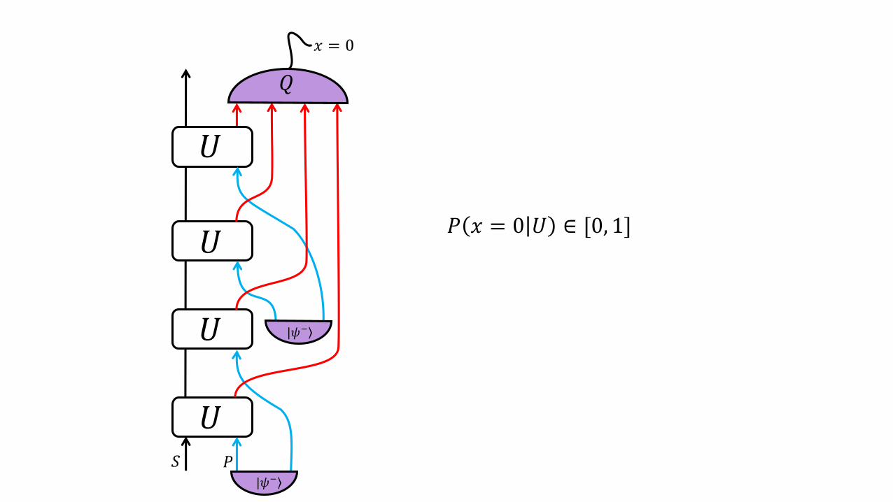
𝑃 𝑥 = 0 𝑈 ∈ [0, 1]
𝑥 = 0
𝑆
𝑈
𝑈
𝑈
𝑈𝑃
𝑄
|𝜓−
|𝜓−
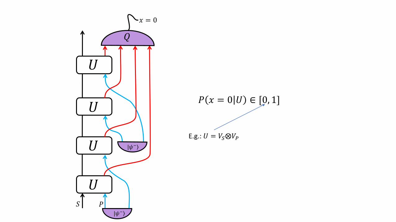
𝑃 𝑥 = 0 𝑈 ∈ [0, 1]
𝑥 = 0
E.g.: 𝑈 = 𝑉𝑆⨂𝑉𝑃
𝑆
𝑈
𝑈
𝑈
𝑈𝑃
𝑄
|𝜓−
|𝜓−
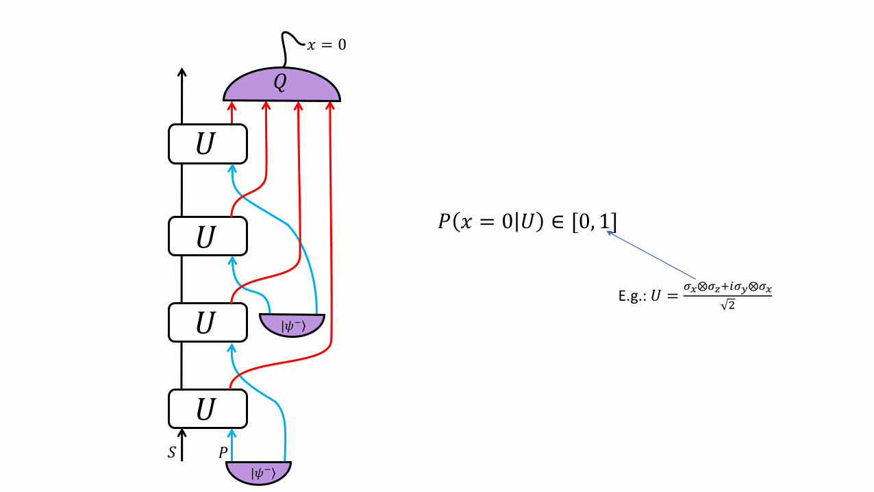
𝑃 𝑥 = 0 𝑈 ∈ [0, 1]
𝑥 = 0
E.g.: 𝑈 =𝜎𝑥⨂𝜎𝑧+𝑖𝜎𝑦⨂𝜎𝑥
2
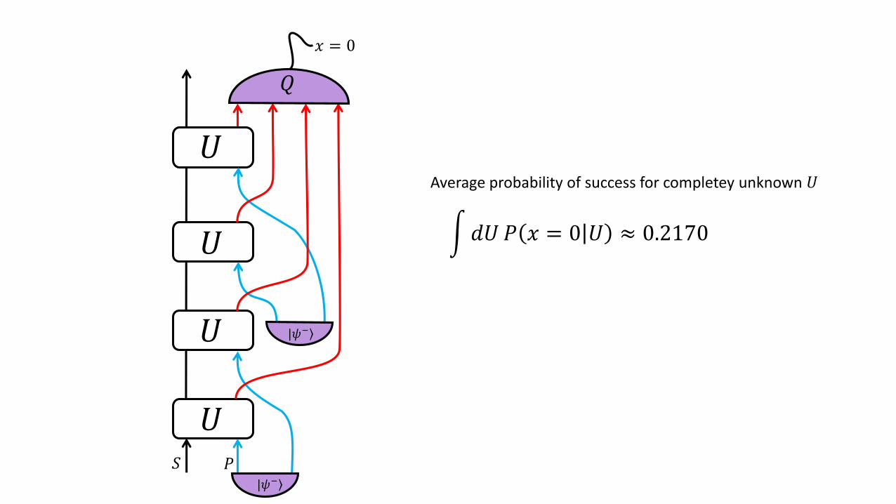
𝑆
𝑈
𝑈
𝑈
𝑈𝑃
𝑄
|𝜓−
|𝜓−
න𝑑𝑈𝑃 𝑥 = 0 𝑈 ≈ 0.2170
Average probability of success for completey unknown 𝑈
𝑥 = 0

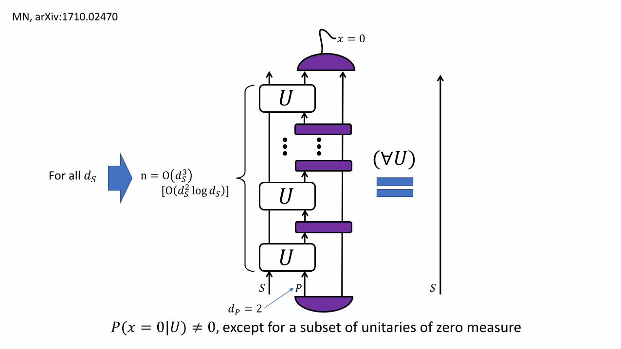
Generalization
𝑆
𝑈
𝑈
𝑈𝑃
(∀𝑈)
𝑆
n = O 𝑑𝑆3
[O 𝑑𝑆2 log 𝑑𝑆 ]
For all 𝑑𝑆
𝑥 = 0
𝑃(𝑥 = 0|𝑈) ≠ 0, except for a subset of unitaries of zero measure
𝑑𝑃 = 2
MN, arXiv:1710.02470
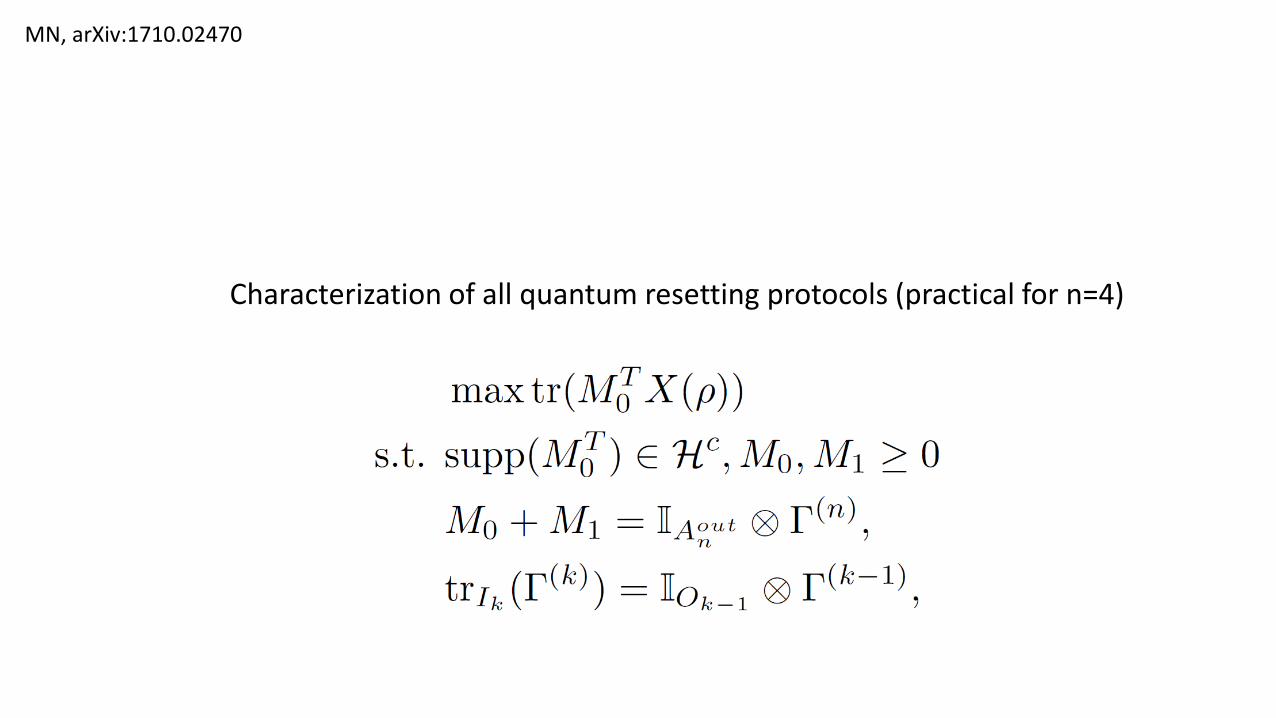
Characterization of all quantum resetting protocols (practical for n=4)
MN, arXiv:1710.02470
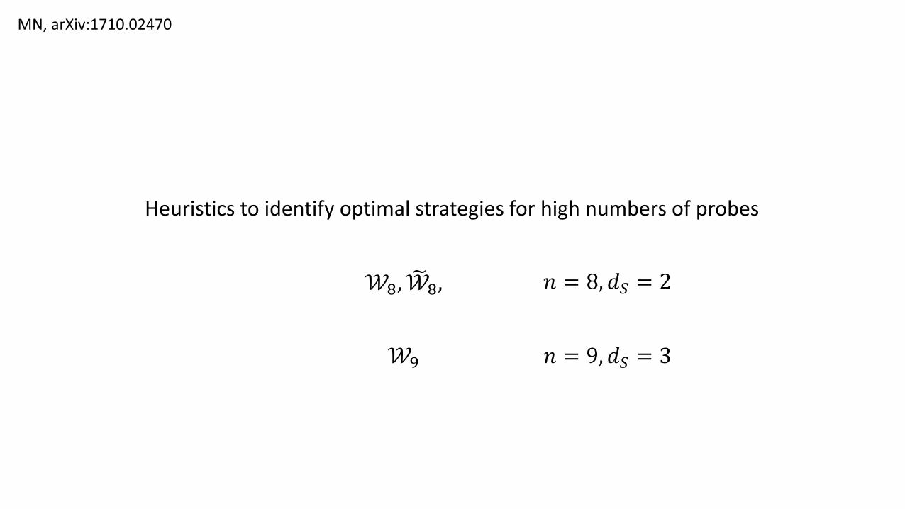
Heuristics to identify optimal strategies for high numbers of probes
𝒲8, ෩𝒲8,
𝒲9
𝑛 = 8, 𝑑𝑆 = 2
𝑛 = 9, 𝑑𝑆 = 3
MN, arXiv:1710.02470

What if the protocol fails?
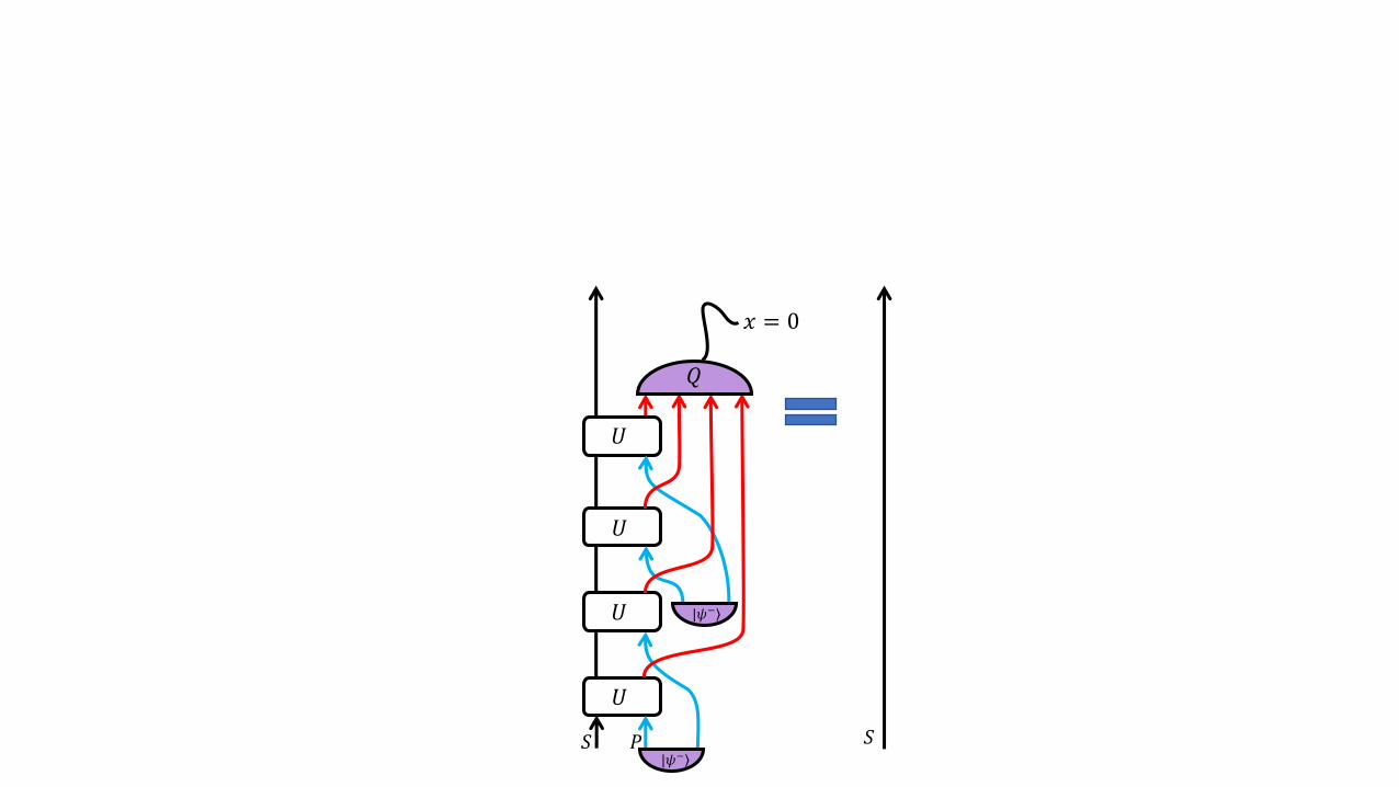
𝑆
𝑈
𝑈
𝑈
𝑈
𝑃
𝑄
|𝜓−
|𝜓−
𝑥 = 0
𝑆
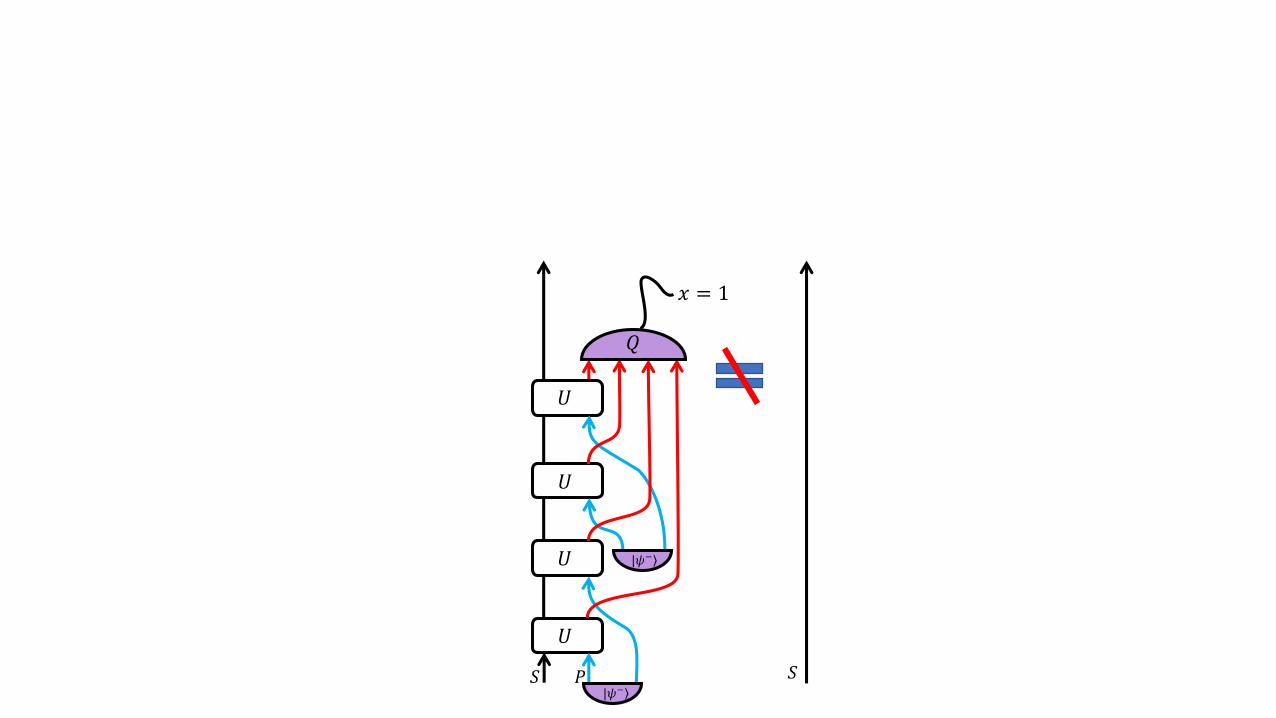
𝑆
𝑈
𝑈
𝑈
𝑈
𝑃
𝑄
|𝜓−
|𝜓−
𝑥 = 1
𝑆
𝑆
𝑈
𝑈
𝑈
𝑈
𝑃
𝑄
|𝜓−
|𝜓−
𝑥 = 1
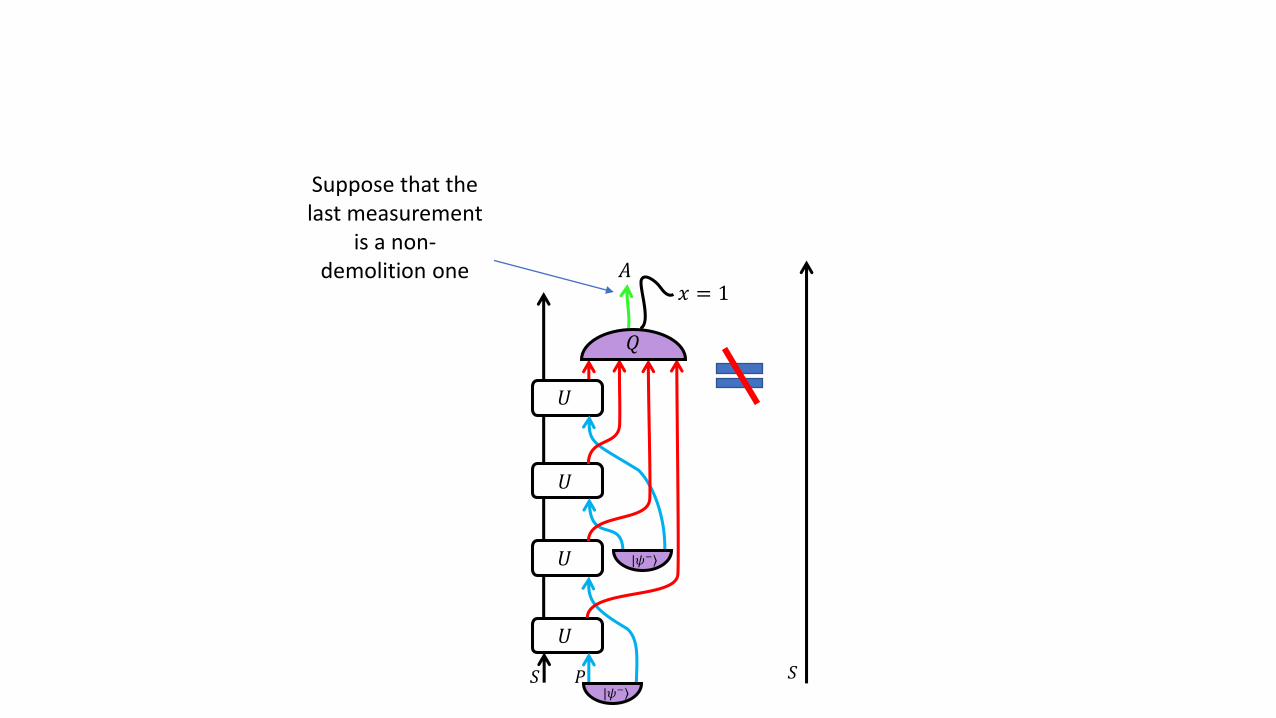
𝑆
Suppose that thelast measurement
is a non-demolition one 𝐴
𝑆
𝑈
𝑈
𝑈
𝑈
𝑃
𝑄
|𝜓−
|𝜓−
|𝜓−
𝑥 = 1
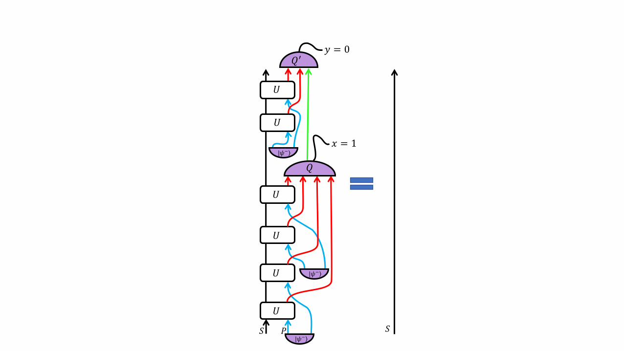
𝑦 = 0
𝑆
𝑈
𝑈
𝑄′

𝑆
𝑈
𝑈
𝑈
𝑈
𝑃
𝑄
|𝜓−
|𝜓−
𝑥 = 1
|𝜔 𝑆𝐴 =
𝑖
𝑓𝑖(𝑈) |𝜓 𝑆 |𝑖 𝐴
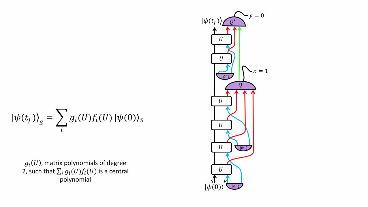
𝑓𝑖 𝑈 , non-central matrix polynomialsof degree 4 on the variables
𝑈𝑖𝑗 = (𝕀𝑆⨂ۦ𝑖|𝑃)𝑈(𝕀𝑆⨂| 𝑗 𝑃)
𝐴
𝑆
𝑈
𝑈
𝑈
𝑈
𝑃
𝑄
|𝜓−
|𝜓−
|𝜓−
𝑥 = 1
𝑦 = 0
𝑈
𝑈
𝑄′
ൿ|𝜓(𝑡𝑓) 𝑆=
𝑖
𝑔𝑖(𝑈)𝑓𝑖(𝑈) |𝜓(0) 𝑆
𝑔𝑖 𝑈 , matrix polynomials of degree2, such that σ𝑖 𝑔𝑖(𝑈)𝑓𝑖(𝑈) is a central
polynomial
ൿ|𝜓(𝑡𝑓)
|𝜓(0)
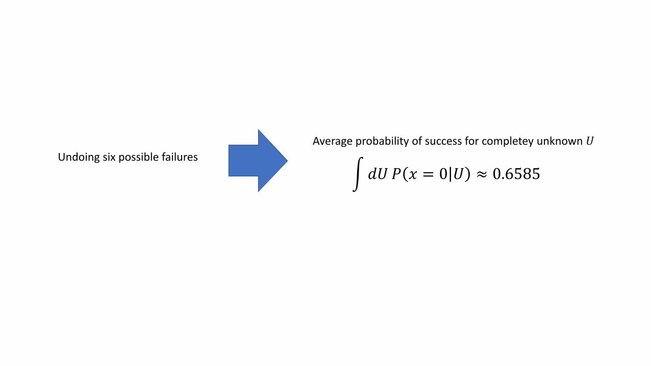
න𝑑𝑈𝑃 𝑥 = 0 𝑈 ≈ 0.6585
Average probability of success for completey unknown 𝑈
Undoing six possible failures

Experimental implementation?
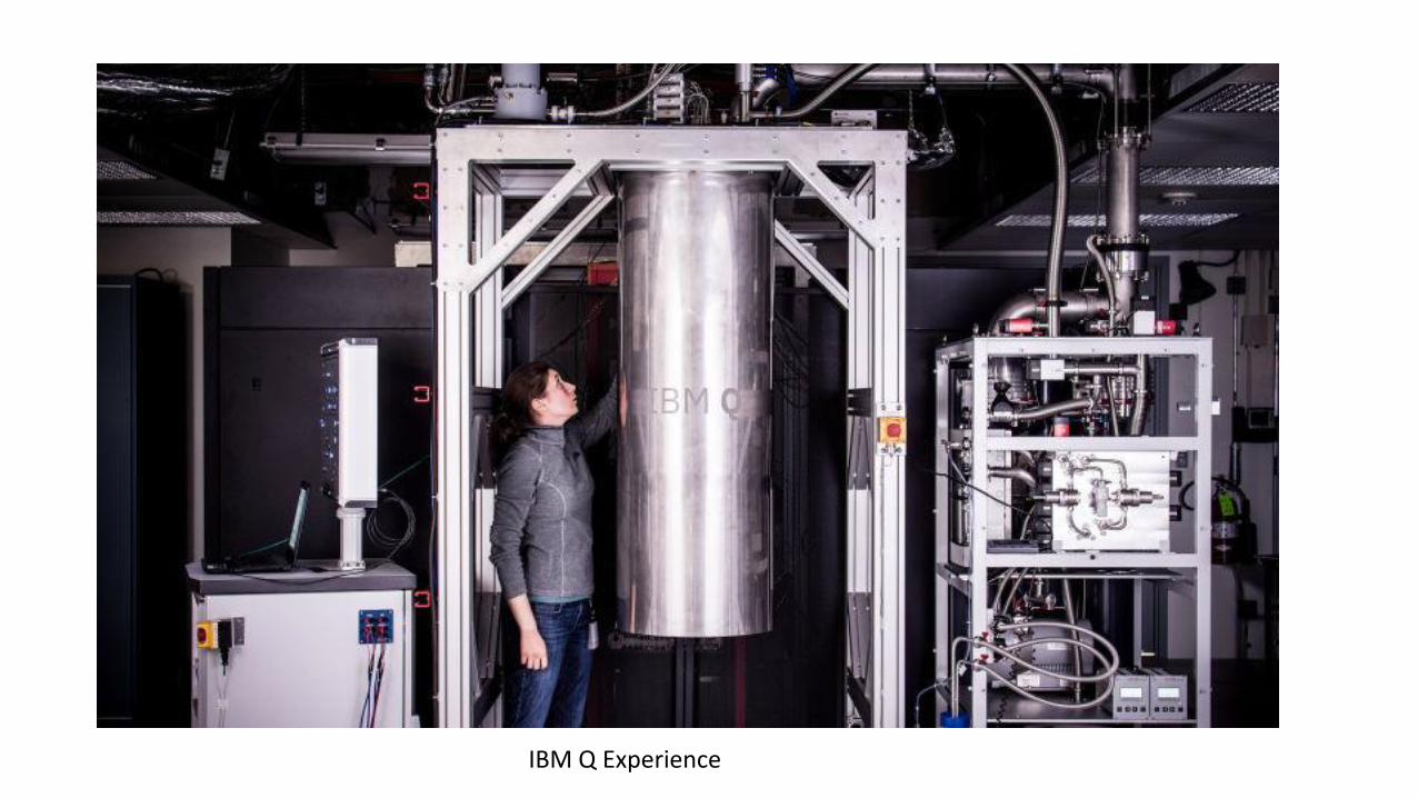
IBM Q Experience
𝑆
𝑈
𝑈
𝑈
𝑈𝑃
𝑄
|𝜓−
|𝜓−
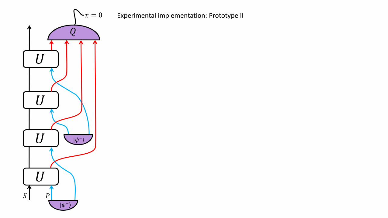
𝑥 = 0 Experimental implementation: Prototype II

𝑆
𝑈
𝑈
𝑈
𝑈𝑃
𝑄
|𝜓−
|𝜓−
𝑥 = 0 Experimental implementation: Prototype II
Implementation with single-qubit gates and CNOTS?
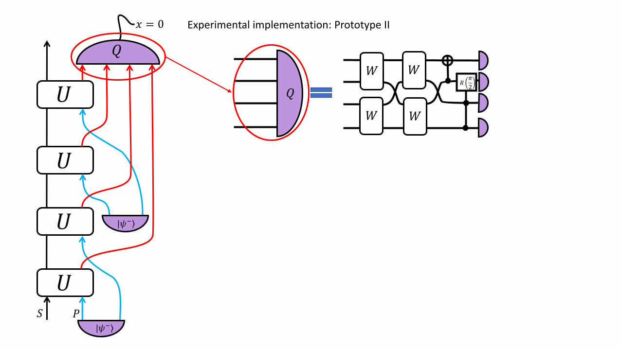
𝑄
𝑊
𝑊
𝑊
𝑊
𝑅𝜋
2
𝑆
𝑈
𝑈
𝑈
𝑈𝑃
𝑄
|𝜓−
|𝜓−
𝑥 = 0 Experimental implementation: Prototype II
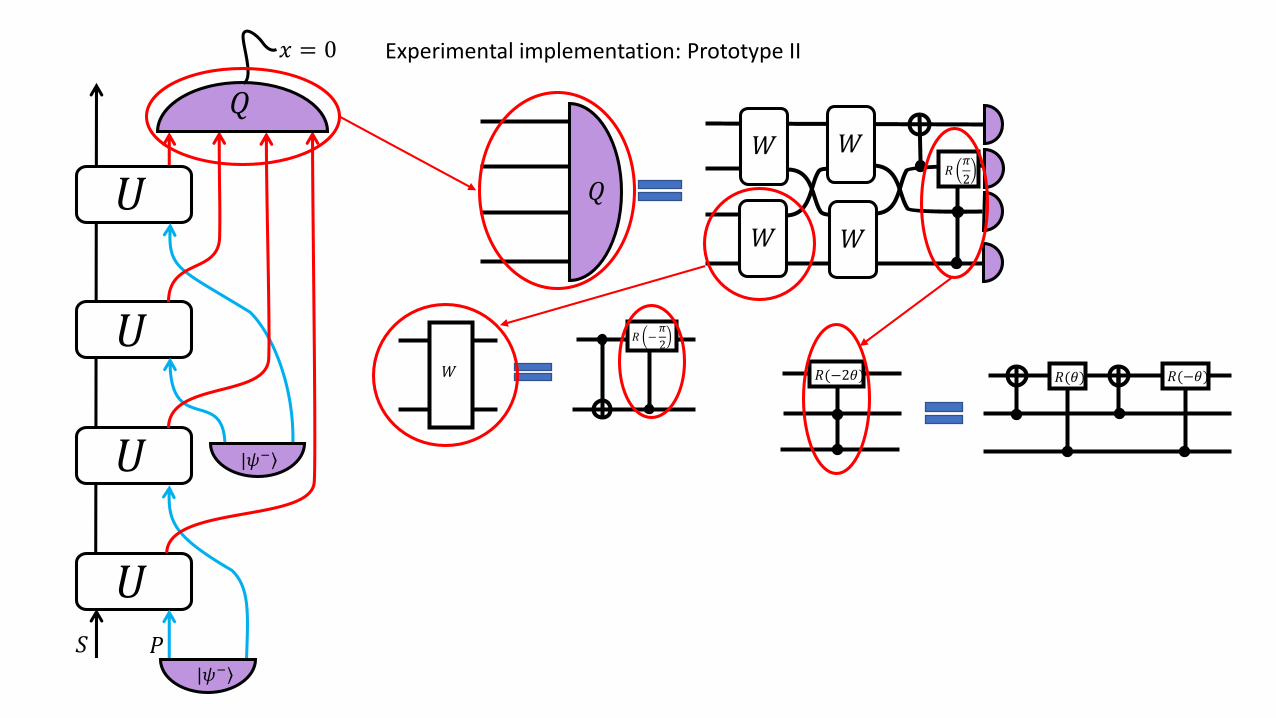
𝑄
𝑊
𝑊
𝑊
𝑊
𝑅𝜋
2
𝑅 −𝜋
2
𝑊
𝑆
𝑈
𝑈
𝑈
𝑈𝑃
𝑄
|𝜓−
|𝜓−
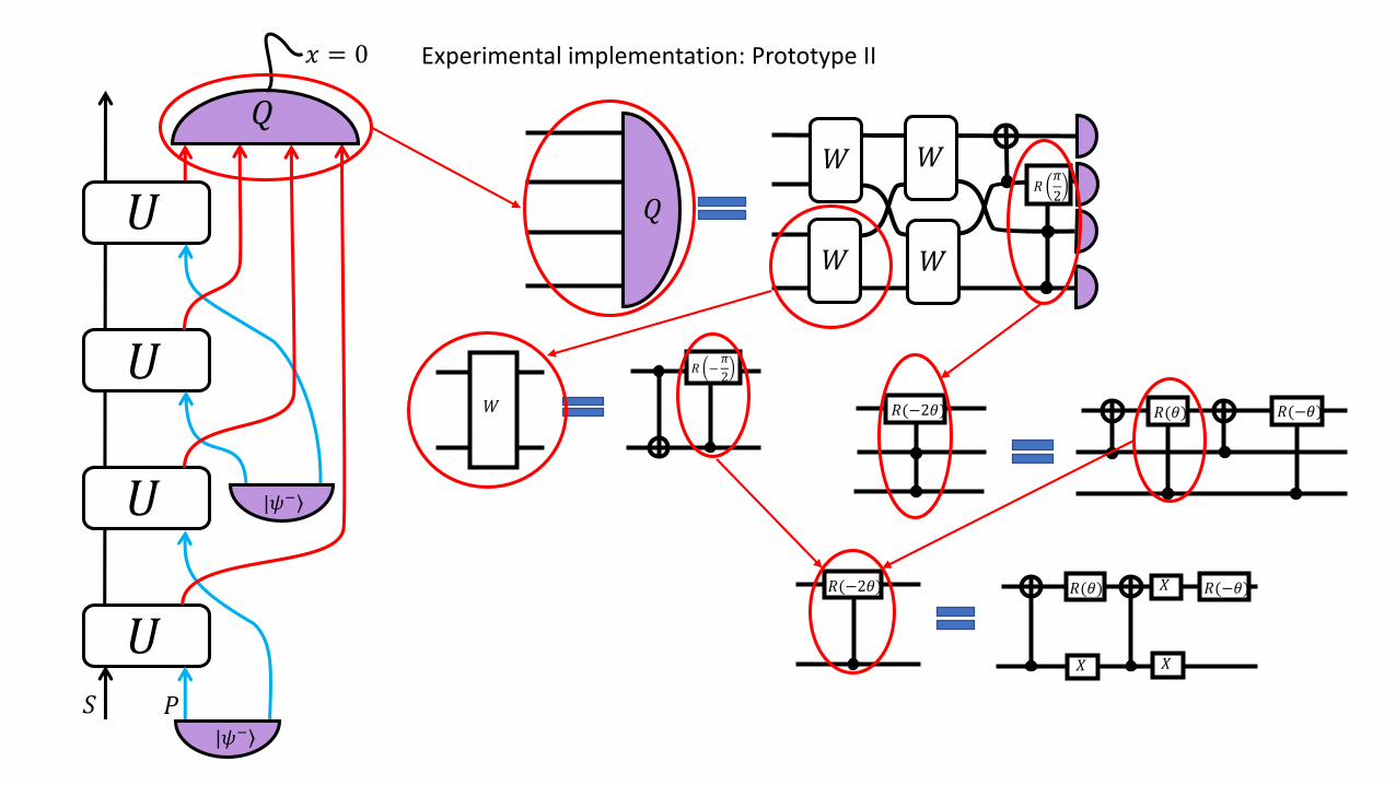
𝑥 = 0 Experimental implementation: Prototype II
𝑅(𝜃) 𝑅(−𝜃)𝑅(−2𝜃)
𝑄
𝑊
𝑊
𝑊
𝑊
𝑅𝜋
2
𝑅 −𝜋
2
𝑊
𝑆
𝑈
𝑈
𝑈
𝑈𝑃
𝑄
|𝜓−
|𝜓−
𝑥 = 0 Experimental implementation: Prototype II
𝑅(𝜃) 𝑅(−𝜃)
𝑋
𝑅(−2𝜃) 𝑋
𝑋
𝑅(𝜃) 𝑅(−𝜃)𝑅(−2𝜃)
𝑄
𝑊
𝑊
𝑊
𝑊
𝑅𝜋
2
𝑅 −𝜋
2
𝑊
𝑆
𝑈
𝑈
𝑈
𝑈𝑃
𝑄
|𝜓−
|𝜓−
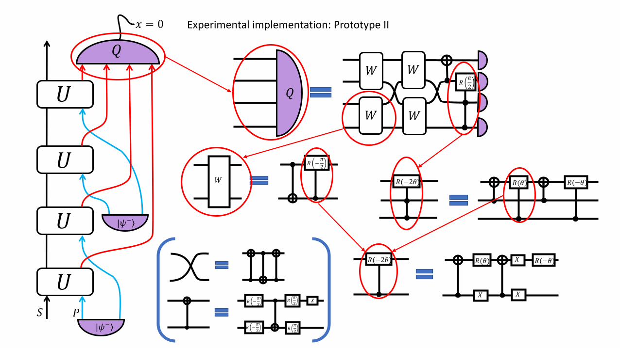
𝑥 = 0 Experimental implementation: Prototype II
𝑅(𝜃) 𝑅(−𝜃)
𝑋
𝑅(−2𝜃) 𝑋
𝑋
𝑅(𝜃) 𝑅(−𝜃)𝑅(−2𝜃)
𝑅 −𝜋
2𝑅
𝜋
2
𝑅 −𝜋
2 𝑅𝜋
2
𝑋
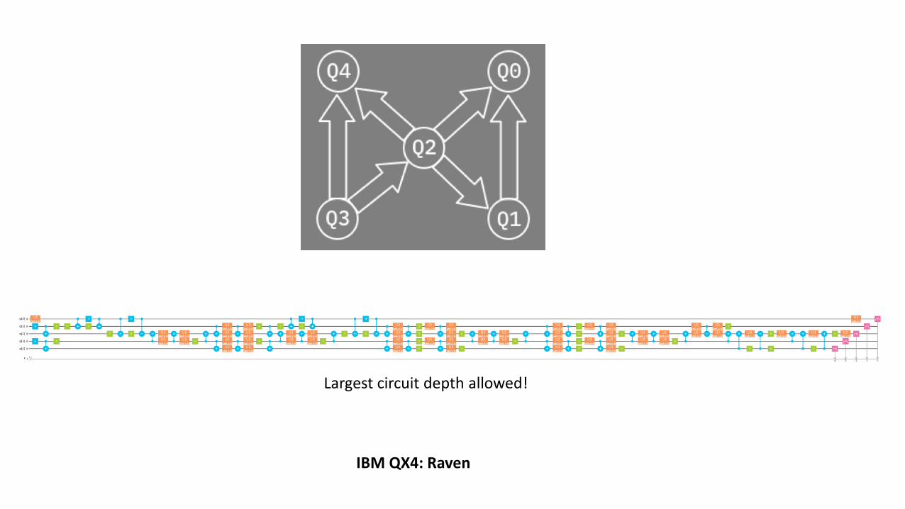
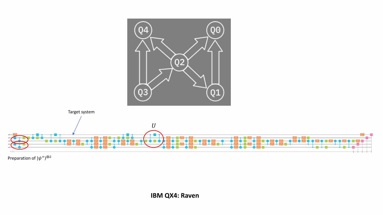
IBM QX4: Raven
Largest circuit depth allowed!
IBM QX4: Raven
Target system
𝑈
Preparation of | 𝜓+ ⨂2
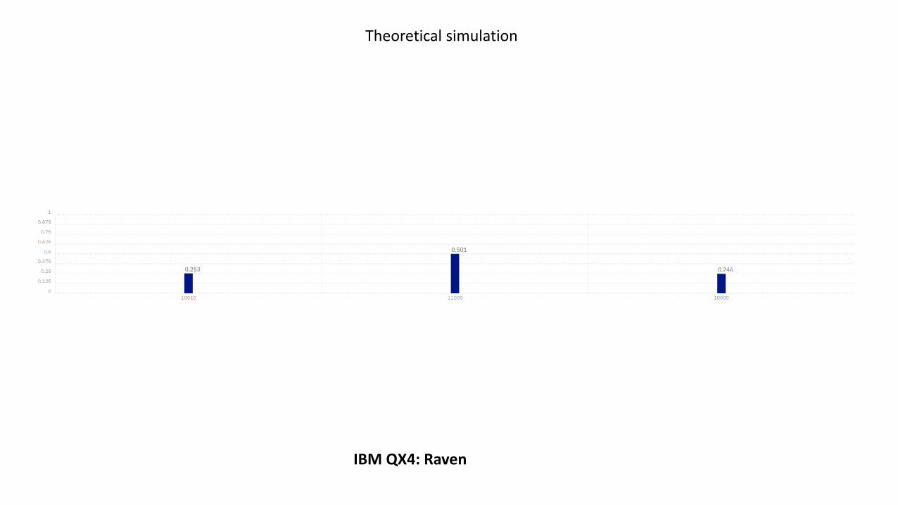
Theoretical simulation
IBM QX4: Raven
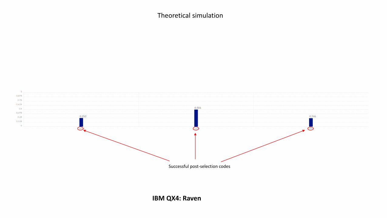
Successful post-selection codes
IBM QX4: Raven
Theoretical simulation
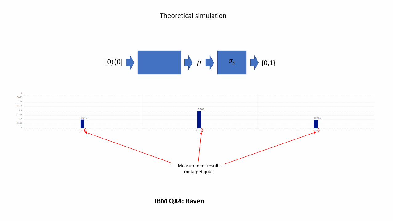
| 0 |0ۦ 𝜌 𝜎𝑧 {0,1}
Measurement resultson target qubit
IBM QX4: Raven
Theoretical simulation
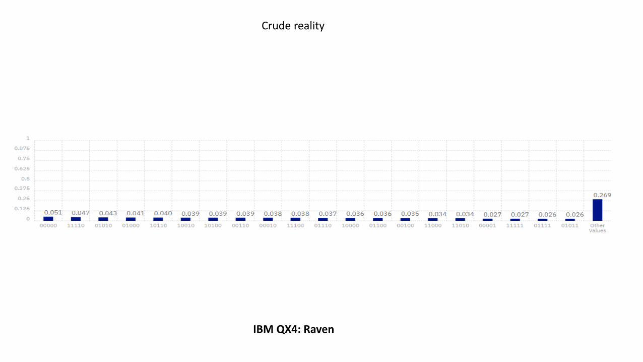
IBM QX4: Raven
Crude reality

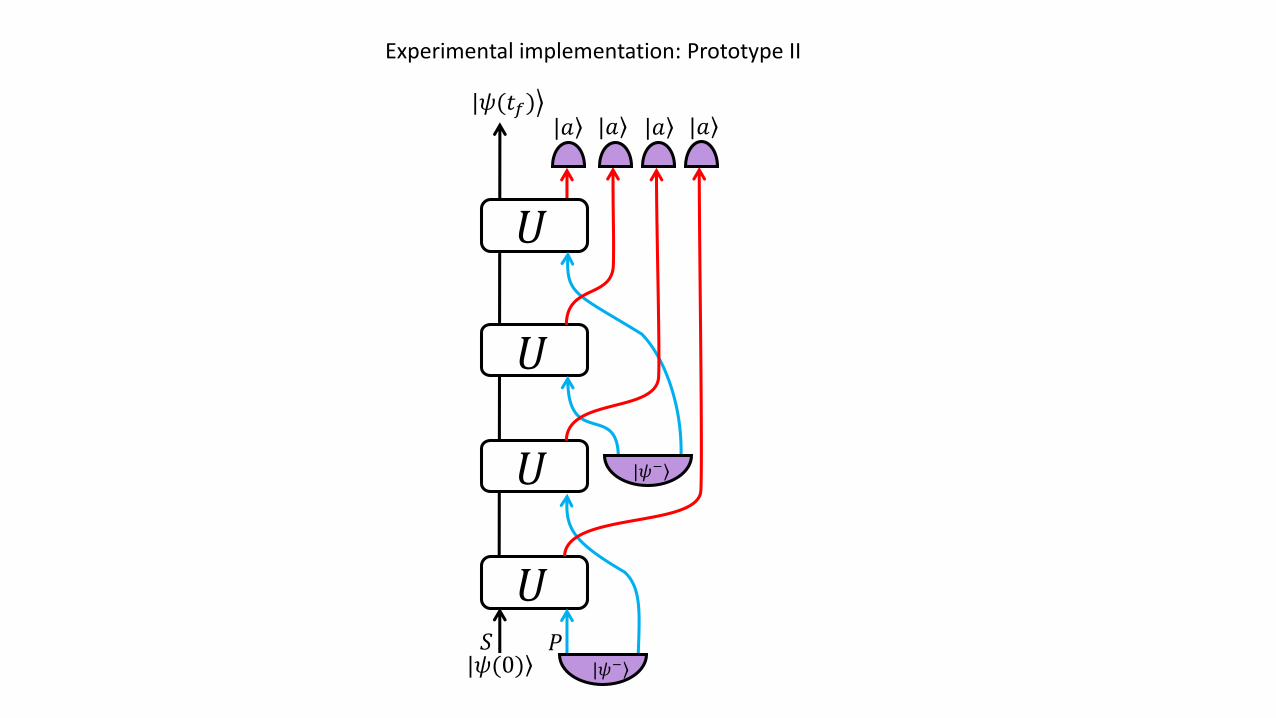
𝑆
𝑈
𝑈
𝑈
𝑈𝑃
|𝜓−
|𝜓−
|𝑎 |𝑎 |𝑎 |𝑎ൿ|𝜓(𝑡𝑓)
|𝜓(0)
Experimental implementation: Prototype II

IBM QX2: Sparrow
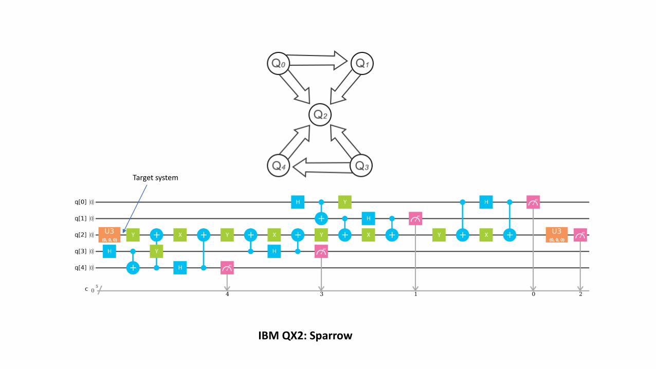
IBM QX2: Sparrow
Target system
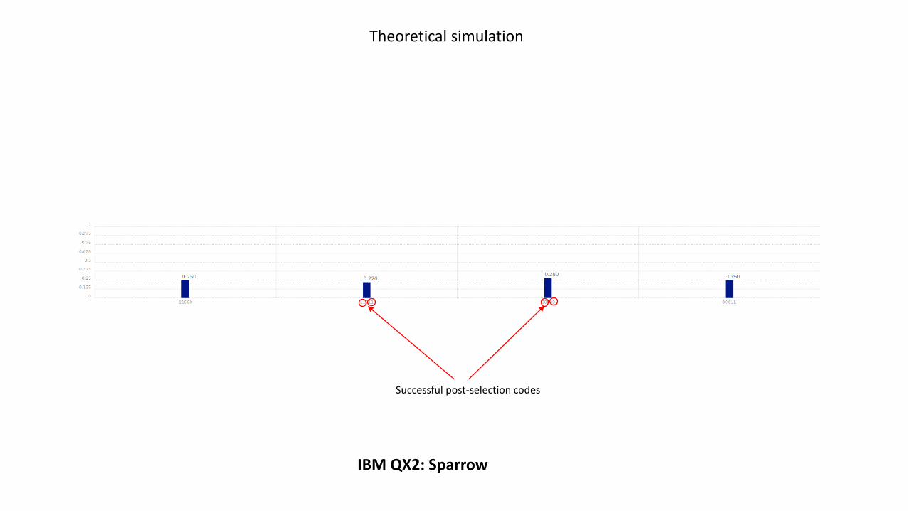
Successful post-selection codes
IBM QX2: Sparrow
Theoretical simulation
IBM QX2: Sparrow
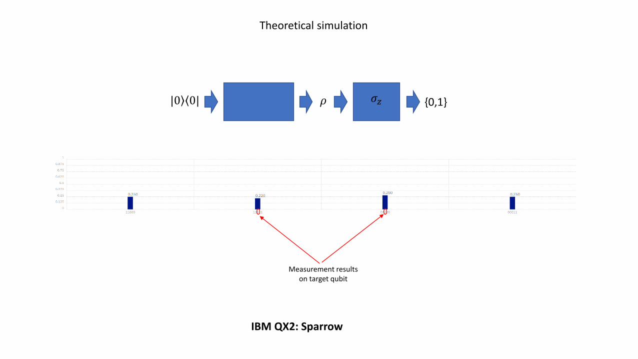
Measurement resultson target qubit
| 0 |0ۦ 𝜌 𝜎𝑧 {0,1}
Theoretical simulation
IBM QX2: Sparrow
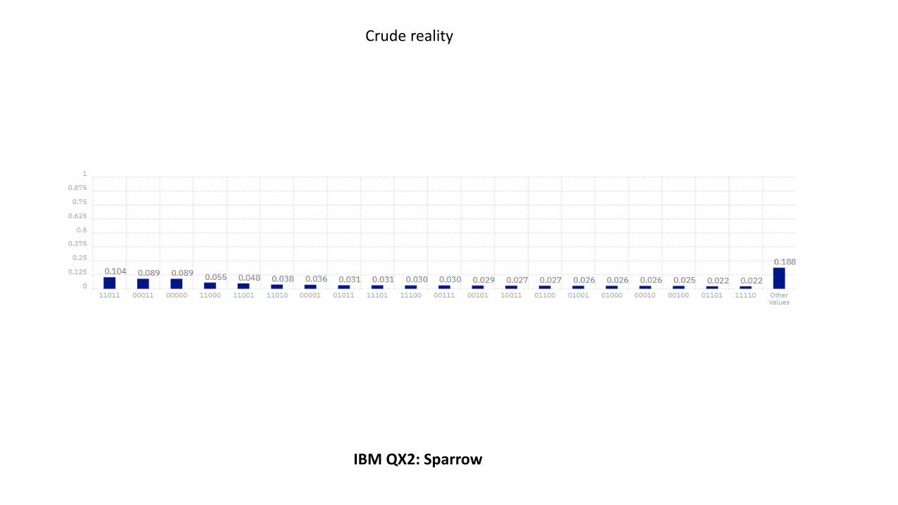
Crude reality

IBM QX2: Sparrow

Conclusion
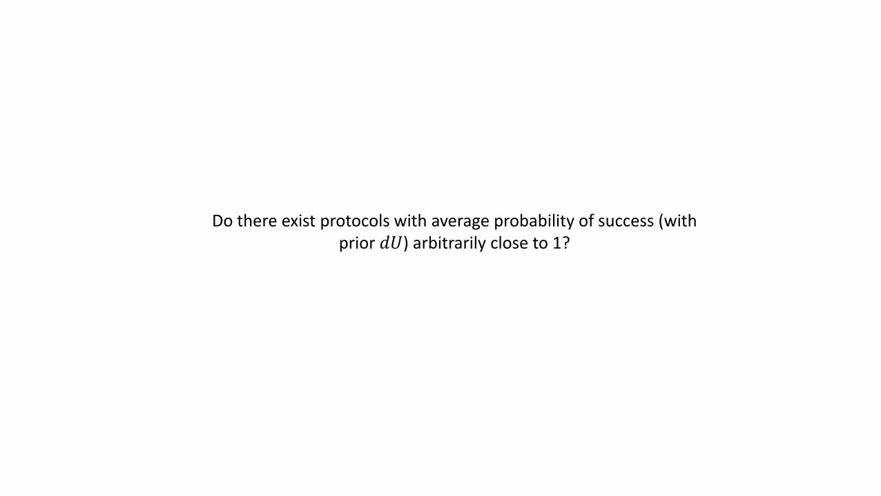
Do there exist protocols with average probability of success (withprior 𝑑𝑈) arbitrarily close to 1?
𝑆
|𝜓(𝑇) = ൿ𝑒−𝑖𝐻0𝑇|𝜓(0)
𝑡 = 𝑇
𝑆
|𝜓(0)
𝑡 = 𝑇 + Δ
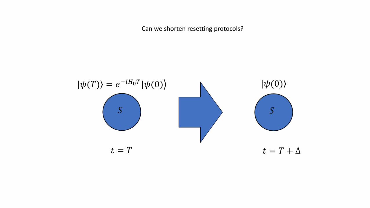
Can we shorten resetting protocols?
𝑆
|𝜓(𝑇) = ൿ𝑒−𝑖𝐻0𝑇|𝜓(0)
𝑡 = 𝑇
𝑆
|𝜓(0)
𝑡 = 𝑇 + Δ
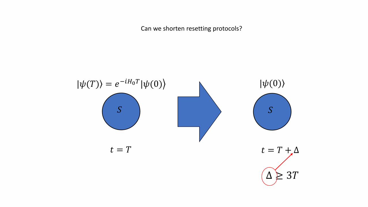
Δ ≥ 3𝑇
Can we shorten resetting protocols?

𝑆
|𝜓(𝑇) = ൿ𝑒−𝑖𝐻0𝑇|𝜓(0)
𝑡 = 𝑇
𝑆
|𝜓(0)
𝑡 = 𝑇 + Δ
Δ ≪ 𝑇?
Can we shorten resetting protocols?
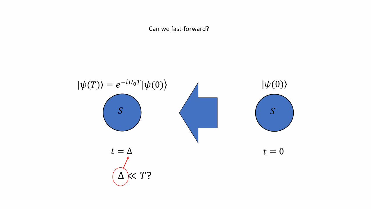
Can we fast-forward?
𝑆
|𝜓(𝑇) = ൿ𝑒−𝑖𝐻0𝑇|𝜓(0)
𝑡 = Δ
𝑆
|𝜓(0)
𝑡 = 0
Δ ≪ 𝑇?
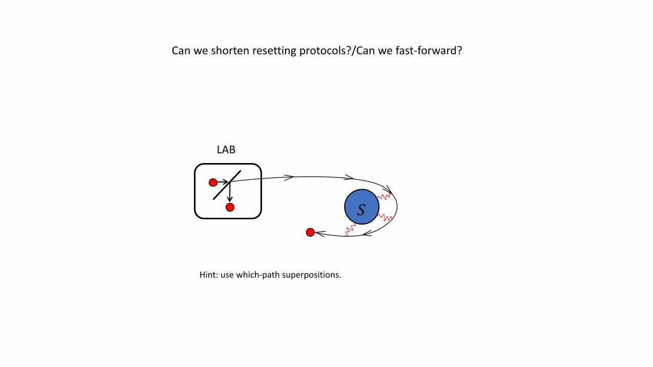
LAB
𝑆
Can we shorten resetting protocols?/Can we fast-forward?
Hint: use which-path superpositions.
Simple experimental implementation?

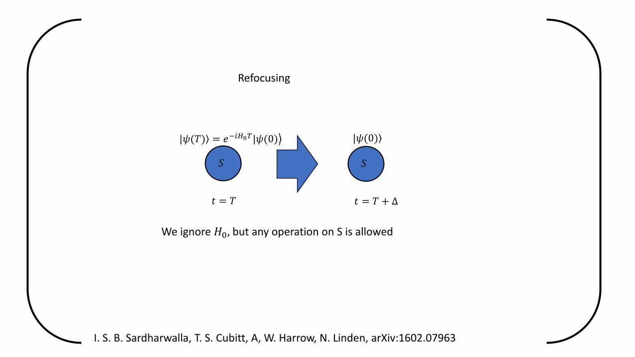
Refocusing
I. S. B. Sardharwalla, T. S. Cubitt, A, W. Harrow, N. Linden, arXiv:1602.07963
𝑆
|𝜓(𝑇) = ൿ𝑒−𝑖𝐻0𝑇|𝜓(0)
𝑡 = 𝑇
𝑆
|𝜓(0)
𝑡 = 𝑇 + Δ
We ignore 𝐻0, but any operation on S is allowed
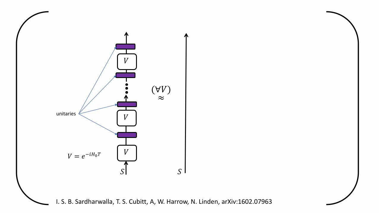
(∀𝑉)
𝑆
𝑉
𝑉
𝑉
≈
unitaries
𝑆
I. S. B. Sardharwalla, T. S. Cubitt, A, W. Harrow, N. Linden, arXiv:1602.07963
𝑉 = 𝑒−𝑖𝐻0𝑇
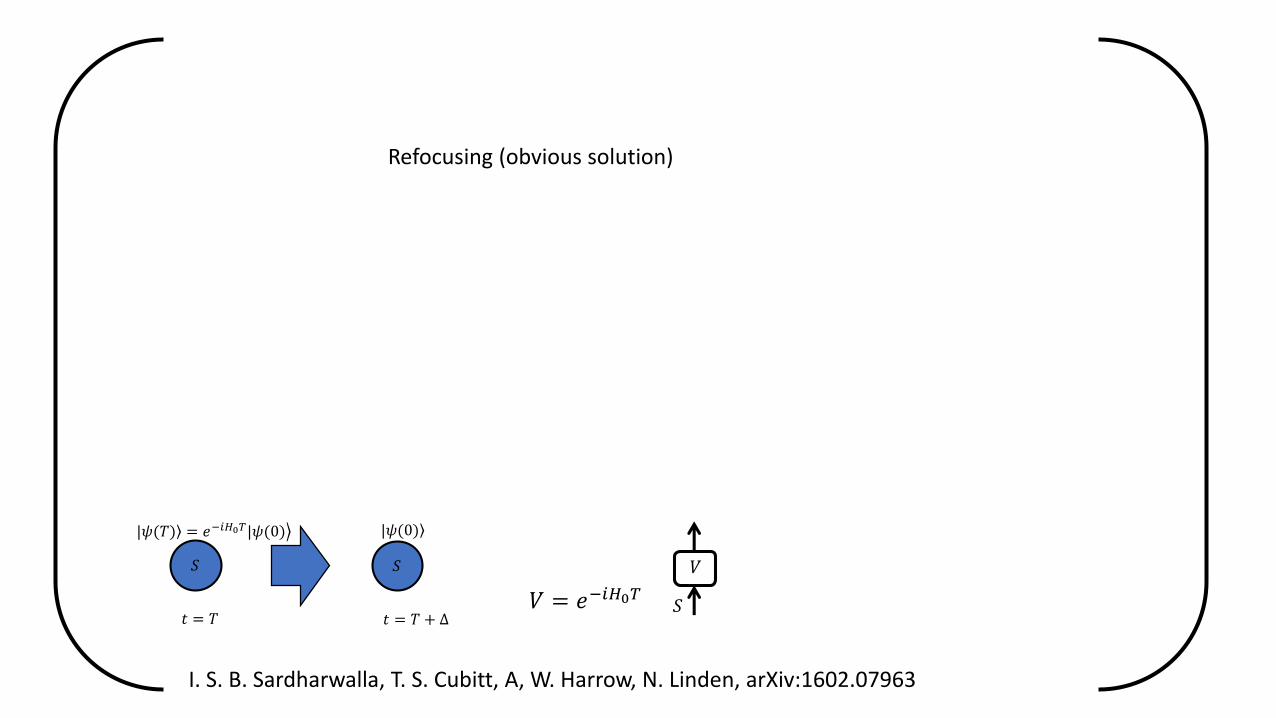
Refocusing (obvious solution)
𝑆
𝑉
𝑉 = 𝑒−𝑖𝐻0𝑇𝑆
|𝜓(𝑇) = ൿ𝑒−𝑖𝐻0𝑇|𝜓(0)
𝑡 = 𝑇
𝑆
|𝜓(0)
𝑡 = 𝑇 + Δ
I. S. B. Sardharwalla, T. S. Cubitt, A, W. Harrow, N. Linden, arXiv:1602.07963

Refocusing (obvious solution)
𝑆
𝑉
𝐴𝑉 = 𝑒−𝑖𝐻0𝑇𝑆
|𝜓(𝑇) = ൿ𝑒−𝑖𝐻0𝑇|𝜓(0)
𝑡 = 𝑇
𝑆
|𝜓(0)
𝑡 = 𝑇 + Δ
I. S. B. Sardharwalla, T. S. Cubitt, A, W. Harrow, N. Linden, arXiv:1602.07963
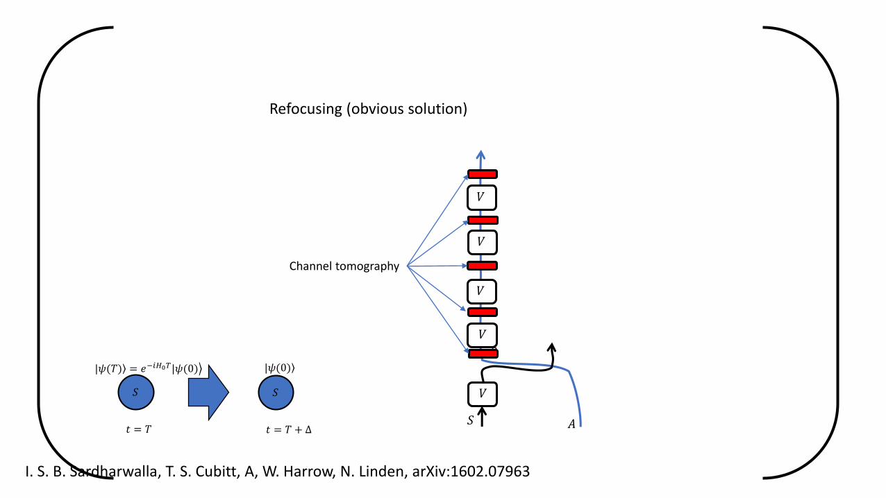
𝑆
𝑆
𝑉
𝑉
𝑉
I. S. B. Sardharwalla, T. S. Cubitt, A, W. Harrow, N. Linden, arXiv:1602.07963
𝑉
𝑉
Channel tomography
𝐴
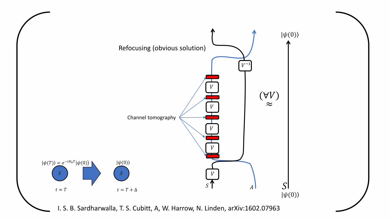
Refocusing (obvious solution)
𝑆
|𝜓(𝑇) = ൿ𝑒−𝑖𝐻0𝑇|𝜓(0)
𝑡 = 𝑇
𝑆
|𝜓(0)
𝑡 = 𝑇 + Δ

𝑆
𝑆
𝑉
𝑉
𝑉
𝑉−1
𝑉
𝑉
Channel tomography
𝐴
Refocusing (obvious solution)
𝑆
|𝜓(𝑇) = ൿ𝑒−𝑖𝐻0𝑇|𝜓(0)
𝑡 = 𝑇
𝑆
|𝜓(0)
𝑡 = 𝑇 + Δ
I. S. B. Sardharwalla, T. S. Cubitt, A, W. Harrow, N. Linden, arXiv:1602.07963
𝑆
𝑆
𝑉
𝑉
𝑉
𝑉−1
𝑉
𝑉
Channel tomography
(∀𝑉)
𝑆
≈
𝐴
Refocusing (obvious solution)
|𝜓(0)
|𝜓(0)
𝑆
|𝜓(𝑇) = ൿ𝑒−𝑖𝐻0𝑇|𝜓(0)
𝑡 = 𝑇
𝑆
|𝜓(0)
𝑡 = 𝑇 + Δ
I. S. B. Sardharwalla, T. S. Cubitt, A, W. Harrow, N. Linden, arXiv:1602.07963


