NIST Technical Note 1782

Residential Carbon Monoxide Exposure due to Indoor Generator Operation: Effects of

Source Location and Emission Rate

Andrew K. Persily Yanling Wang Brian Polidoro

Steven J Emmerich

NIST Technical Note 1782

Residential Carbon Monoxide Exposure due

to Indoor Generator Operation: Effects of Source Location and Emission Rate

Andrew K. Persily Yanling Wang Brian Polidoro

Steven J Emmerich Energy and Environment Division

Engineering Laboratory

June 2013

U.S. Department of Commerce Cameron F. Kerry, Acting Secretary

National Institute of Standards and Technology

Patrick D. Gallagher, Under Secretary of Commerce for Standards and Technology and Director

Certain commercial entities, equipment, or materials may be identified in this document in order to describe an experimental procedure or concept adequately.

Such identification is not intended to imply recommendation or endorsement by the National Institute of Standards and Technology, nor is it intended to imply that the entities, materials, or equipment are necessarily the best available for the purpose.

National Institute of Standards and Technology Technical Note 1782 Natl. Inst. Stand. Technol. Tech. Note 1782, 47 pages (June 2013)

CODEN: NTNOEF

iii

ABSTRACT The U.S. Consumer Product Safety Commission (CPSC) and others are concerned about the hazard of acute residential carbon monoxide (CO) exposures from portable gasoline powered generators that can result in death or serious adverse health effects in exposed individuals. CPSC databases contain records of 755 deaths from CO poisoning associated with consumer use of generators in the period of 1999 through 2011, with nearly three-quarters of those occurring between 2005 and 2011 [1]. The majority of these incidents occur during power outages, or when a generator is used to provide power to a structure that is not wired for electrical power. Typically, these deaths occur when consumers use a generator in an enclosed or partially enclosed space or outdoors near an open door, window or vent. While avoiding the operation of such generators in or near a home is expected to reduce indoor CO exposures significantly, it may not be realistic to expect such usage to be eliminated completely. Another means of reducing these exposures would be to decrease the amount of CO emitted from these devices. In order to support life-safety based analyses of potential CO emission limits, a computer simulation study was conducted to evaluate indoor CO exposures as a function of generator source location and CO emission rate. These simulations employed the multizone airflow and contaminant transport model CONTAM, which was applied to a collection of 87 single-family, detached dwellings that are representative of the U.S. housing stock for that housing type. A total of almost one hundred thousand individual 24-hour simulations were conducted. This report presents the simulation results in terms of the maximum levels of carboxyhemoglobin that would be experienced by occupants in the occupied portions of the dwellings as a function of CO emission rate for different indoor source locations. KEYWORDS: carbon monoxide; CONTAM; emergency generators; multizone airflow model; simulation

iv

TABLE OF CONTENTS 1. INTRODUCTION 1 2. ANALYSIS METHOD 1 2.1 Description of homes 1 2.2 Modeling approach 3 2.2.1 CONTAM model 3 2.2.2 Baseline house models 3 2.2.3 Source locations and emission rates 6 2.2.4 Simulation cases and output analysis 7 3. RESULTS 9 3.1 House airtightness and air change rates 9 3.2 Detailed results for one detached house (DH-10) 11 3.3 Summary results for all houses 14 3.4 Summary results for subsets of houses 20 4. SUMMARY AND DISCUSSION 24 5. ACKNOWLEDGEMENTS 26 6. REFERENCES 26 APPENDICES A. House Characteristics 28 B. Source Locations for Each House 32 C. Integral Mass Balance Analysis of Burst Sources 35 D. Cumulative Frequency Distributions of MaxCOHb in Tabular Form 38

1

1. INTRODUCTION The U.S. Consumer Product Safety Commission (CPSC) and others are concerned about the hazard of acute residential carbon monoxide (CO) exposures from portable gasoline-powered generators, which can result in death or serious adverse health effects in exposed individuals. CPSC databases contain records of 755 deaths from CO poisoning associated with consumer use of generators in the period of 1999 through 2011, with nearly three-quarters of those occurring between 2005 and 2011 [1]. The majority of these incidents occur during power outages, or when a generator is used to provide power to a structure that is not wired for electrical power. Typically, these deaths occur when consumers use a generator in an enclosed or partially enclosed space or outdoors near a partially open door, window or vent. While avoiding the operation of such generators in or near a home is expected to reduce indoor CO exposures significantly, it may not be realistic to expect such usage to be eliminated completely. Another means of reducing these exposures would be to decrease the amount of CO emitted from these devices. The magnitude of such reductions needed to reduce exposures to some specific level depends on the complex relationship between CO emissions from these generators and occupant exposure. Technically achievable levels of CO emissions reduction have been studied by NIST through an experimental investigation of CO emissions from generators in a shed and a house. These investigations included measurements on prototype generators that were modified to reduce their CO emission rates [2]. That study provided a set of unique measurements of CO emission rates for both unmodified and modified generators. The issue of how CO emission rates relate to occupant exposure involves the interaction between generator operation, house characteristics, occupant activity, and weather conditions. In order to support life-safety based analyses of potential CO emission limits for generators, a computer simulation study was conducted to evaluate indoor CO exposures as a function of generator source location and CO emission rate. These simulations employed the multizone airflow and contaminant transport model CONTAM [3], which was applied to a collection of 87 single-family, detached dwellings that are representative of the U.S. housing stock for that housing type. A total of almost one hundred thousand individual 24-hour simulations were conducted. This report presents the simulation results in terms of the maximum levels of percent carboxyhemoglobin (COHb) that would be experienced by occupants in the occupied portions of the dwellings as a function of CO emission rate for different indoor source locations. 2. ANALYSIS METHOD This section describes the approach used to perform the simulations, including the houses that were considered, the simulated generator locations and CO emission rates, and the manner in which the simulations were performed and the output analyzed. In designing this study, the goal was to be reasonably conservative in terms of the assumptions and inputs employed. Decisions about the assumptions and inputs used in the analysis were made not to result in worst-case conditions (highest CO exposures), but rather to tend towards higher exposures while still being realistic and technically sound. 2.1 Description of homes The homes used in the simulations are based on a collection of dwellings that were previously defined by Persily et al. [4], which includes just over 200 dwellings that together represent 80 % of the U.S. housing stock. Those dwellings are grouped into four categories: detached (83 homes),

2

attached (53 homes), manufactured homes (4) and apartments (69). The definition of this set of dwellings was based on the following variables using the US Census Bureau’s American Housing Survey (AHS) [5] and the US Department of Energy’s (DOE) Residential Energy Consumption Survey (RECS) [6]: housing type, number of stories, heated floor area, year built, foundation type, presence of a garage, type of heating equipment, number of bedrooms, number of bathrooms, and number of other rooms. In addition to defining the dwellings, multizone representations were created in the airflow and contaminant transport model CONTAM to support their use in analyzing a range of ventilation and indoor air quality issues [3]. Only the detached and manufactured home models were used in this analysis, for a total of 87 homes. The attached and apartment models were not employed based on the challenge in accounting for airflow between units and the lack of air leakage data for the partitions between units. Given the prevalence of single-family dwellings within the U.S. housing stock, these 87 homes represent on the order of 60 % of U.S. dwellings. Appendix A summarizes the characteristics of the 87 dwellings included in the analysis and identifies the corresponding CONTAM project file name and associated floor plan. The project files and floor plans can be downloaded at the CONTAM website www.bfrl.nist.gov/IAQanalysis under Case Studies. However, as discussed below, these files were modified for the purposes of this analysis. In constructing this collection of dwellings, the year of construction was used to assign the exterior wall leakage based on data from studies of the airtightness in single-family homes [7-9]. Exterior wall leakage is commonly defined in terms of the normalized leakage area, which for these dwellings is a function of the year built and house floor area as presented in Table 1 [4]. The normalized leakage (NL) values from this table are converted to an effective leakage area (ELA) for use in the house models based on the following equation [10]:

𝑁𝐿 = 1000 𝐸𝐿𝐴𝐴𝑓� 𝐻2.5�

0.3 (1)

where, Af is the floor area in m2

and H is the building height in m.

Normalized leakage area (dimensionless)

Year built Floor area less than 148.6 m2

(1600 ft2) Floor area greater than

148.6 m2 (1600 ft2)

Before 1940 1.29 0.58 1940-1969 1.03 0.49 1970-1989 0.65 0.36

1990 and newer 0.31 0.24 Table 1 Normalized leakage by construction year and floor area

In developing the house models used in this study, the conditioned floor area of each house was used in conjunction with Table 1 to determine its ELA value by solving Equations (1) for ELA. The value of ELA was calculated using the NL from the table, and Af and H for the house. The floor area used in this calculation did not include garages, attics and unfinished basements.

3

2.2 Modeling approach Using this set of homes, indoor CO concentrations were calculated using the multizone airflow and contaminant transport model CONTAM [3] over a range of source (generator) locations, CO emission rates, and weather conditions. As described below, these simulations yielded CO concentrations in the rooms of each house as a function of time during the analysis interval. In order to compare the results for different cases, the concentrations from each simulation were then used to calculate COHb values for an occupant spending the full 24 hours in each room. The maximum COHb (maxCOHb) value among the occupied rooms of the house was used as a metric of CO exposure for that house, source and weather scenario. This section describes the manner in which these simulations were conducted and the results were analyzed. 2.2.1 CONTAM model As noted previously, the indoor CO concentrations were calculated using the multizone airflow and contaminant transport model CONTAM [3]. CONTAM is a simulation tool for predicting airflows and contaminant concentrations in multizone building airflow systems. When using CONTAM, a building is represented as a series of interconnected zones (e.g. rooms), with the airflow paths (e.g., leakage sites and doorways) between the zones and the outdoors defined as mathematical relationships between the airflow through the path and the pressure difference across it. Outdoor weather conditions are also input into CONTAM, as they are key determinants of pressure differences across airflow paths in exterior walls. System airflow rates must also be defined to capture their effects on building and interzone pressure differences. These inputs are used to define mass balances of air into and out of each zone, which are solved simultaneously to determine the interzone pressures relationships and resulting airflow rates between each zone, including the outdoors. These airflow rates can be calculated over time as weather conditions and system airflow rates change. Once the airflows are established, CONTAM can then calculate contaminant concentrations over time in each building zone based on contaminant source characteristics and contaminant removal information, such as that associated with filtration. CONTAM has been used for several decades, and a range of validation studies have demonstrated its ability to reliably predict building air change rates and contaminant levels [11, 12]. 2.2.2 Baseline house models The models used in this analysis were based on the 83 detached and 4 manufactured homes described above. In general, these models were used as previously defined. However, a number of decisions on their configuration were required as well as some limited modifications. Air handling system operation: While many of the 87 homes in this collection include air handling systems for heating and cooling, this analysis was based on the assumption that the forced-air distribution systems were not operating. The limited electrical output of these generators reduces the likelihood that whole-house space conditioning systems will be operating. Also, forced-air system operation will increase ventilation rates [10], thereby reducing CO concentrations. Therefore, having the system off is consistent with the goal of the analysis being reasonably conservative. In addition, all local exhaust fans (kitchen and bath) were assumed to be off. Wind exposure: A CONTAM model of a building must be associated with a coefficient to account for the impacts of surrounding terrain, buildings and vegetation on wind-induced pressures on the exterior façade of the building. CONTAM describes three categories of terrain including flat,

4

exposed areas (e.g., airport), suburban and dense urban centers. A user can input coefficients to describe terrain options in between the flat and urban extremes. These simulations employed the suburban category of terrain shielding, which corresponds to areas with obstructions of the size and spacing of single-family homes. The houses were oriented such that the predominant wind direction for the simulated weather conditions was directed into the garage door. This orientation was used so as to increase the transport of CO from the garage of the house, consistent with the goal of being reasonably conservative. Weather conditions: Each house and generator source combination was analyzed for 28 individual days, with each CO release event occurring at the beginning of each 24-h analysis period. Each of the 28 simulations employed a different day of weather conditions, including outdoor temperature, wind speed and wind direction, that varied on an hourly basis. The 28 days of weather correspond to two weeks of cold weather, one week of warm and one week of mild. The hourly weather data were based on weather files for the following three cities: Detroit MI (cold), Miami FL (warm) and Columbus OH (mild). The files were obtained from the EnergyPlus Energy Simulation Software website: http://apps1.eere.energy.gov/buildings/energyplus/cfm/weather_data.cfm. Table 2 presents a summary of the weather conditions for the 28 days in the form of daily average, minimum and maximum outdoor temperatures and wind speeds. Summary values are also included for the cold, mild and warm days separately. Indoor air temperatures: The indoor temperature was held constant at 23 °C (73.4 °F) in all interior zones during all of the simulations with the following exceptions. The air temperature in zones containing the generators was assumed to increase linearly over two hours from 23 °C (73.4 °F) to 40 °C (104 °F). After the generator stopped operating, the temperature was assumed to decrease linearly over six hours back to 23 °C (73.4 °F). The air temperature in zones adjacent to the zone containing the generator was assumed to increase on the same schedule but only to 30 °C (86 °F). These indoor air temperature changes are based on the results of a series of experimental studies of generator operation conducted at NIST [2]. These temperature schedules were applied to the constant source cases (described below). In the burst source simulations (also described below), the generator was assumed to release all of the associated CO over a very short period of time and no change in the interior temperatures was simulated. The indoor air temperatures of unconditioned spaces, i.e., crawl spaces, unfinished basements, garages and attics, were held constant 23 °C (73.4 °F). This assumption does not capture temperature variations in such unconditioned spaces based on weather and interaction with the outdoors. However, the use of a constant temperature greatly simplifies the analysis and generally serves to reduce the driving forces of building air change, consistent with the reasonably conservative simulation approach. Door and window positions: All interior doors were assumed to be open during the simulations and all exterior doors and windows closed with the following exceptions. When the generator was located in an unfinished basement, the door between the basement and the upstairs was closed. Finished basements had an open stairway between the basement and the first floor, and all interior doors on both levels were open. For cases in which the generator was located in the attached garage, the door from the garage to the house was assumed be open roughly 5 cm (2 in.) to accommodate an extension cord running from to the generator. When the generator was in the garage with the garage door open, the open garage door was modeled as an opening 4.6 m (15 ft.) wide and 0.6 m (2 ft.) high.

5

Day Outdoor temperature, °C (°F) Wind speed, m/s (mph)

Average Minimum Maximum Average Minimum Maximum Cold 1-Jan 0.7 (33.3) -1.7 (28.9) 5.6 (42.1) 3.2 (7.2) 0.0 (0.0) 5.7 (12.8) 2-Jan 6.1 (43.1) 0.0 (32.0) 12.2 (54.0) 3.9 (8.8) 2.1 (4.7) 5.7 (12.8) 3-Jan 2.5 (36.6) 1.1 (34.0) 4.4 (39.9) 3.1 (6.8) 2.1 (4.7) 4.1 (9.2) 4-Jan 0.9 (33.6) 0.0 (32.0) 1.7 (35.1) 2.9 (6.6) 0.0 (0.0) 4.6 (10.3) 5-Jan -2.9 (26.8) -5.0 (23.0) 0.0 (32.0) 5.8 (13.1) 4.1 (9.2) 8.2 (18.3) 6-Jan -3.3 (26.1) -5.0 (23.0) -1.7 (28.9) 5.2 (11.6) 1.5 (3.4) 8.2 (18.3) 7-Jan -3.8 (25.2) -6.1 (21.0) -2.2 (28.0) 3.2 (7.2) 0.0 (0.0) 5.2 (11.6) 8-Jan -1.7 (28.9) -3.3 (26.1) 0.0 (32.0) 2.4 (5.3) 0.0 (0.0) 5.2 (11.6) 9-Jan -0.1 (31.8) -1.7 (28.9) 1.1 (34.0) 3.5 (7.7) 1.5 (3.4) 6.2 (13.9)

10-Jan 1.8 (35.3) 1.0 (33.8) 2.8 (37.0) 3.5 (7.7) 0.0 (0.0) 6.7 (15.0) 11-Jan 0.6 (33.0) -0.6 (30.9) 1.1 (34.0) 4.3 (9.5) 0.0 (0.0) 5.7 (12.8) 12-Jan 4.9 (40.7) 0.6 (33.1) 13.3 (55.9) 3.9 (8.7) 0.0 (0.0) 8.8 (19.7) 13-Jan 9.2 (48.5) 0.6 (33.1) 14.4 (57.9) 6.4 (14.3) 2.6 (5.8) 10.3 (23.0) 14-Jan -5.5 (22.2) -9.4 (15.1) 1.1 (34.0) 5.3 (11.9) 2.6 (5.8) 7.2 (16.1)

Mild 3-Apr 6.0 (42.7) 2.8 (37.0) 8.3 (46.9) 6.9 (15.5) 0.0 (0.0) 9.8 (21.9) 4-Apr 6.3 (43.3) -0.6 (30.9) 13.3 (55.9) 2.1 (4.7) 0.0 (0.0) 5.7 (12.8) 5-Apr 9.0 (48.1) 1.1 (34.0) 15.6 (60.1) 1.8 (4.0) 0.0 (0.0) 3.6 (8.1) 6-Apr 11.9 (53.4) 5.0 (41.0) 18.9 (66.0) 3.7 (8.3) 2.1 (4.7) 6.2 (13.9) 7-Apr 16.2 (61.1) 11.1 (52.0) 22.8 (73.0) 5.4 (12.1) 0.0 (0.0) 12.4 (27.7) 8-Apr 11.0 (51.8) 7.0 (44.6) 13.9 (57.0) 6.0 (13.5) 0.0 (0.0) 9.8 (21.9) 9-Apr 8.5 (47.3) 3.9 (39.0) 13.3 (55.9) 5.5 (12.4) 0.0 (0.0) 8.2 (18.3)

Warm 25-Jul 28.5 (83.2) 25.6 (78.1) 33.3 (91.9) 2.5 (5.7) 1.0 (2.2) 5.2 (11.6) 26-Jul 29.3 (84.8) 25.0 (77.0) 35.0 (95.0) 3.4 (7.6) 1.5 (3.4) 7.2 (16.1) 27-Jul 29.5 (85.2) 25.0 (77.0) 35.0 (95.0) 2.5 (5.7) 1.5 (3.4) 6.2 (13.9) 28-Jul 30.0 (86.1) 25.6 (78.1) 35.6 (96.1) 3.0 (6.7) 1.0 (2.2) 5.2 (11.6) 29-Jul 28.5 (83.3) 25.6 (78.1) 33.9 (93.0) 3.3 (7.3) 1.0 (2.2) 11.3 (25.3) 30-Jul 29.2 (84.5) 26.1 (79.0) 33.3 (91.9) 3.0 (6.7) 1.0 (2.2) 6.2 (13.9) 31-Jul 29.0 (84.1) 27.8 (82.0) 31.7 (89.1) 4.3 (9.6) 0.0 (0.0) 8.2 (18.3)

Average values for weather periods

Cold days 0.7 (33.2) -2.1 (28.2) 3.8 (38.9) 4.0 (9.0) 1.2 (2.6) 6.6 (14.7) Mild days 9.8 (49.7) 4.3 (39.8) 15.2 (59.3) 4.5 (10.1) 0.3 (0.7) 8.0 (17.8)

Warm days 29.1 (84.5) 25.8 (78.5) 34.0 (93.1) 3.1 (7.0) 1.0 (2.2) 7.1 (15.8)

Table 2 Summary of Hourly Weather Data Used in Simulations

6

2.2.3 Source locations and emission rates The range of potential CO generation scenarios for indoor operation of generators in actual homes is very large. Given the goals of being reasonably conservative and avoiding excessive complexity, the simulated source scenarios covered only a well-defined range. Two types of sources were considered: a constant CO generation rate lasting 18 hours; and, a short “burst” of CO intended to represent a generator with some form of CO emission control technology (e.g. a shut off device) for which a constant generation rate is not a reasonable assumption. The constant generation rate for the first type of source and the mass released by the second used in the simulations covered a range of values based on measurements and analyses conducted by CPSC and NIST. The source scenarios that were analyzed include the following: Constant generation rate for 18 hours with the source in the following locations: Closed garage (if applicable to the model house) Open garage (if applicable to the model house) Basement (if applicable to the model house) Interior room (on first floor) Short term burst source with the source in the following locations: Closed garage (if applicable to the model house) Basement (if applicable to the model house) Interior room (on first floor) The interior room for each house was selected from those rooms defined by the existing floor plans of the model homes employed, with the goal of selecting a room on the first floor where a generator could be expected to be located. The interior rooms are identified by their CONTAM “zone name” in Appendix B, which lists the zone names of the constant and burst sources in each of the simulated houses. In some cases these locations are identified as bathrooms, however this selection is based on the zones in the existing CONTAM models and is not intended to suggest the bathroom as a likely generator location. The interior rooms were selected based on their locations on the first floor and not on their designation in the existing models. The simulated CO emission rates for the constant (in units of g/h) and the burst (units of total mg released) sources are contained in Table 3 and Table 4 respectively, along with an explanation of each value. The short term burst source values are based on an integral mass balance analysis of generator tests conducted at NIST, which is described in Appendix C of this document. For all of the simulations the outdoor CO concentration was assumed to equal zero, since the indoor concentrations of interest are well above typical ambient levels.

7

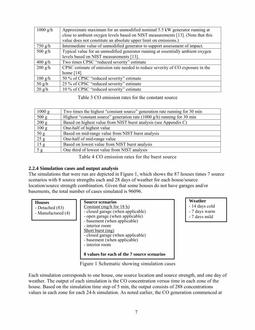
1000 g/h Approximate maximum for an unmodified nominal 5.5 kW generator running at close to ambient oxygen levels based on NIST measurements [13]. (Note that this value does not constitute an absolute upper limit on emissions.)

750 g/h Intermediate value of unmodified generator to support assessment of impact. 500 g/h Typical value for an unmodified generator running at essentially ambient oxygen

levels based on NIST measurements [13]. 400 g/h Two times CPSC “reduced severity” estimate 200 g/h CPSC estimate of emission rate needed to reduce severity of CO exposure in the

home [14] 100 g/h 50 % of CPSC “reduced severity” estimate 50 g/h 25 % of CPSC “reduced severity” estimate 20 g/h 10 % of CPSC “reduced severity” estimate

Table 3 CO emission rates for the constant source

1000 g Two times the highest “constant source” generation rate running for 30 min 500 g Highest “constant source” generation rate (1000 g/h) running for 30 min 200 g Based on highest value from NIST burst analysis (see Appendix C) 100 g One-half of highest value 50 g Based on mid-range value from NIST burst analysis 25 g One-half of mid-range value 15 g Based on lowest value from NIST burst analysis 5 g One third of lowest value from NIST analysis

Table 4 CO emission rates for the burst source 2.2.4 Simulation cases and output analysis The simulations that were run are depicted in Figure 1, which shows the 87 houses times 7 source scenarios with 8 source strengths each and 28 days of weather for each house/source location/source strength combination. Given that some houses do not have garages and/or basements, the total number of cases simulated is 96096.

Figure 1 Schematic showing simulation cases Each simulation corresponds to one house, one source location and source strength, and one day of weather. The output of each simulation is the CO concentration versus time in each zone of the house. Based on the simulation time step of 5 min, the output consists of 288 concentrations values in each zone for each 24-h simulation. As noted earlier, the CO generation commenced at

Houses - Detached (83) - Manufactured (4)

Weather - 14 days cold - 7 days warm - 7 days mild

Source scenarios Constant (mg/h for 18 h) - closed garage (when applicable) - open garage (when applicable) - basement (when applicable) - interior room Short burst (mg) - closed garage (when applicable) - basement (when applicable) - interior room 8 values for each of the 7 source scenarios

8

the beginning of each 24-h period. In the case of the constant source, the CO generation stopped 18 hours later, after which the indoor CO concentrations started decreasing back to ambient levels. COHb levels were calculated for an occupant in each occupied zone of the house over the 24-h simulation period using the Coburn-Forster-Kane (CFK) equation [15, 16] and input values provided by CPSC, specifically an RMV (respiratory minute volume) of 15 L/min and an initial COHb level of 0.0024 ml/ml. The maximum COHb (maxCOHb) value among the occupied zones of each house was used as the output metric for each simulation. The maxCOHb values were considered separately for each source location to generate a frequency distribution for each source/location combination. Fifty-six such distributions were generated from the simulation results, i.e., seven locations times eight source strengths per location. In order to assess the impact of house size, airtightness, and weather conditions, subsets of the detached house results were considered separately. With respect to house size, separate frequency distributions were generated for the 37 detached homes in the smallest size category, for the 16 homes in the largest size category and for the remaining 30 “mid-sized” homes. These size categories correspond to conditioned floor areas of 107.4 m2 (1152 ft2), 180.4 m2 (1942 ft2), and 275.5 m2 (2966 ft2), respectively for the small, mid-sized and large detached homes. Note that all of the manufactured houses are the same size, i.e., 86.3 m2 (929 ft2), and their results were also considered separately. In order to assess the impact of house airtightness, separate frequency distributions of maxCOHb were generated for the 20 tightest and 20 leakiest detached houses. The identification of these tight and leaky homes is based on the air change rate at an indoor-outdoor pressure difference of 50 Pa (0.2 in. H2O), which is determined by simulating a building pressurization (blower door) test using CONTAM. Finally, the impacts of weather were examined for the detached houses by generating separate frequency distributions of maxCOHb for the two cold weeks of weather, one week of mild weather, and one week of warm weather.

9

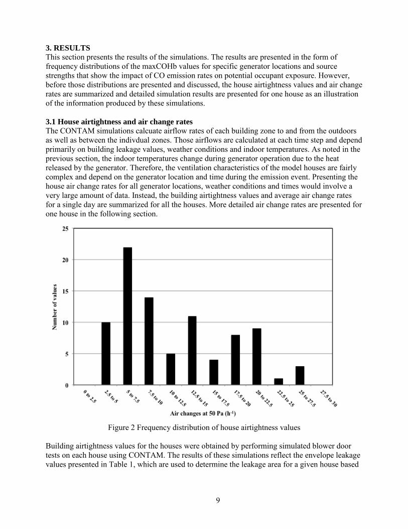
3. RESULTS This section presents the results of the simulations. The results are presented in the form of frequency distributions of the maxCOHb values for specific generator locations and source strengths that show the impact of CO emission rates on potential occupant exposure. However, before those distributions are presented and discussed, the house airtightness values and air change rates are summarized and detailed simulation results are presented for one house as an illustration of the information produced by these simulations. 3.1 House airtightness and air change rates The CONTAM simulations calcuate airflow rates of each building zone to and from the outdoors as well as between the indivdual zones. Those airflows are calculated at each time step and depend primarily on building leakage values, weather conditions and indoor temperatures. As noted in the previous section, the indoor temperatures change during generator operation due to the heat released by the generator. Therefore, the ventilation characteristics of the model houses are fairly complex and depend on the generator location and time during the emission event. Presenting the house air change rates for all generator locations, weather conditions and times would involve a very large amount of data. Instead, the building airtightness values and average air change rates for a single day are summarized for all the houses. More detailed air change rates are presented for one house in the following section.

Figure 2 Frequency distribution of house airtightness values Building airtightness values for the houses were obtained by performing simulated blower door tests on each house using CONTAM. The results of these simulations reflect the envelope leakage values presented in Table 1, which are used to determine the leakage area for a given house based

10

on its age and size. CONTAM is then run for each house in a mode that determines the airflow required to pressurize the house to a given reference pressure difference between the indoors and outdoors. The airflow is then normalized by the building volume to yield the common airtightness metric of air changes per hour at 50 Pa. The results of these simulations are presented in Figure 2, which is a frequency distribution of the building air change rate at an indoor-outdoor pressure difference of 50 Pa. The values for the 87 houses range from 3.6 h-1 to 25.6 h-1, with a mean of 11.4 h-1 and a standard deviation of 6.2 h-1. Note that these air change rates correspond to an elevated test pressure under a simulated pressurization test and are therefore much higher than the air change rates induced by weather and normal building operation.

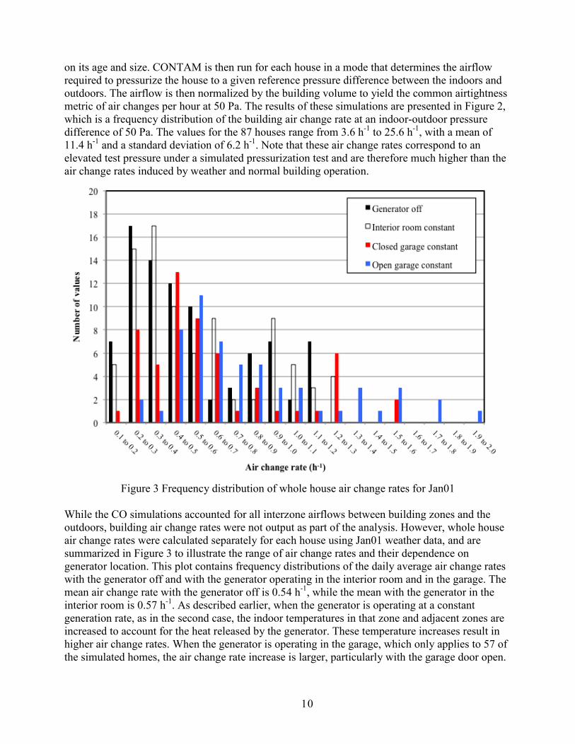
Figure 3 Frequency distribution of whole house air change rates for Jan01 While the CO simulations accounted for all interzone airflows between building zones and the outdoors, building air change rates were not output as part of the analysis. However, whole house air change rates were calculated separately for each house using Jan01 weather data, and are summarized in Figure 3 to illustrate the range of air change rates and their dependence on generator location. This plot contains frequency distributions of the daily average air change rates with the generator off and with the generator operating in the interior room and in the garage. The mean air change rate with the generator off is 0.54 h-1, while the mean with the generator in the interior room is 0.57 h-1. As described earlier, when the generator is operating at a constant generation rate, as in the second case, the indoor temperatures in that zone and adjacent zones are increased to account for the heat released by the generator. These temperature increases result in higher air change rates. When the generator is operating in the garage, which only applies to 57 of the simulated homes, the air change rate increase is larger, particularly with the garage door open.

11

The mean daily average air change rate with the generator operating at a constant rate in a closed garage is 0.62 h-1, while the mean with the generator in the open garage is 0.82 h-1. 3.2 Detailed results for one detached house (DH-10) This section presents simulation results for detached house DH-10 as an example of the detailed information produced by the CONTAM modeling. This particular house was selected because it has both a garage and a basement, but its results are not presented as being representative of the larger group of homes. Figure 4 shows a floor plan of the house. For this house the CO sources were located in the garage (closed and open), Bathroom 2 in the basement, and the ½ Bath on the first floor (as the interior room source). As noted earlier, these bathrooms source locations are based on the zones in the existing CONTAM models and not on their designation as bathrooms.

Figure 4 Floor plan of house DH-10 As noted earlier, the house air change rates vary with weather conditions (outdoor temperature, wind speed and wind direction). In addition, the indoor air temperature changes when the generator is running as a constant source (due to the heat released from the generator) also impact the air change rates. To illustrate these impacts, Figure 5 contains frequency distributions for the hourly air change rates in house DH10 for all 28 days of

12

weather with no generator running and with the generator running in the garage (closed) and in the interior room, both in the constant source mode. The hourly air change rates with the generator off range from 0.06 h-1 to 0.62 h-1, with a mean of 0.25 h-1. Due to the increase in indoor temperatures with the generator running, the air change rates are larger with the constant sources, as seen in Figure 5. With the generator in the closed garage, the air change rate ranges from 0.07 h-1 to 0.90 h-1, with a mean of 0.36 h-1. With the generator running in the interior room, the air change rates also increase relative to the generator-off case, but are less than for the closed garage case.

Figure 5 Frequency distribution of air change rates in DH10 with generator off and on

13

Figure 6 shows the predicted CO concentrations in the kitchen zone for DH-10 with the generator in the closed garage and a constant source of 1000 g/h. Each line corresponds to the concentrations for one of the 28 days of simulated weather, with each day identified as cold, mild or warm. This plot highlights the variability in the predicted CO concentrations for the different days, which supports the use of multiple days of weather to obtain a better characterization of the CO exposure than could be obtained using any particular day. Simulation results for only a single day are highly dependent on the specific weather conditions, particularly wind speed and direction, and could lead to potential misinterpretations relative to considering a wide range of weather conditions.

Figure 6 DH-10 CO concentrations in kitchen for 1000 g/h source in closed garage Table 5 presents average predicted values of daily maximum and daily mean CO concentrations in house DH-10 for a constant source of 1000 g/h, which is a high-end value for an unmodified generator as discussed earlier. Average values of the daily maximum and mean concentrations are included for all four generator locations. Concentrations for each occupied room are contained in Table 5 and show the impact of source location. For example, when the generator is in the garage, the highest average concentrations are on the first floor. For this generator location, the basement concentrations are much lower than on other levels, regardless of the garage door position. With the generator in the garage, significant amounts of CO reach the basement only during warm weather conditions due to the downward stack effect that exists when the indoor temperature is lower than outdoors. When the generator is in the basement, the highest concentrations are in the

14

zones on that level. The CO concentrations in the basement and interior room locations are well above those when the generator in the garage, since in the latter cases much of the CO dissipates to the outdoors before entering the house. In contrast, when the generator is in the basement or the interior room, all of the CO enters the house. Note that this table only includes the occupied zones of the building and not the bathroom and stairway zones.

CO CONCENTRATIONS (mg/m3) Closed

Garage Open

Garage Basement Interior Room

Max Mean Max Mean Max Mean Max Mean Level Zone Basement Bed3 6 2 104 61 13259 8209 1564 791

Bed4 8 3 11 3 23893 15596 2309 1325 1st floor Kitchen 2555 1448 471 291 7153 3825 5723 2956

Living 2326 1315 465 284 5214 2894 14650 8940 Dining 2421 1371 467 287 9765 5475 5732 2962

2nd floor Bed1 511 246 324 194 5816 3675 6995 4157 Bed2 456 213 308 186 5882 3511 8020 4708

Table 5 Average of daily maximums and means CO concentrations for 1000 g/h constant sources in DH-10

3.3 Summary results for all houses This section presents the results of the COHb calculations for all of the houses considered in the simulations, which reflect the combined effects of source location, source strength and weather conditions. As noted earlier, the metric employed in analyzing the simulation results is the maximum COHb value (maxCOHb) among the occupied zones for each simulation. Each maxCOHb value corresponds to a 24-hour simulation of a specific house (among the 87 houses considered) for a specific source location, source strength and day of weather. For reference, COHb levels of 70 % or greater are associated with death in less than 3 min, levels of 50 % are associated with headache, dizziness and nausea in 5 min to 10 min and death within 30 min, levels of 30 % with dizziness, nausea and convulsions within 45 min and becoming insensible within 2 h, and levels of 20 % with a slight headache in 2 h to 3 h and a loss of judgment [17]. Figure 7 shows example results with the generator in the interior room for two values of a constant CO source, 1000 g/h and 100 g/h. In both plots the solid vertical bars correspond to the percent of values among all of the simulations (all houses and weather conditions) for which the maxCOHb is in each bin on the horizontal axis. For example, in the upper plot corresponding to 1000 g/h, there are a small fraction of cases with maxCOHb value between 0 % and 5 %; all the rest have maxCOHb values above 80 %. The small number of cases with max COHb below 5 % occurs when essentially all of the CO produced by the generator leaves the house without flowing into the occupied rooms. In those cases, the maxCOHb corresponds to the assumed initial COHb concentration used in the CFK calculation, i.e. 0.0024 ml/ml. No maxCOHb bins are presented above 80 % because distinctions between such high levels are not of interest based on health effects at such high levels. The solid line in each graph is the cumulative distribution of the maxCOHb values, which always reaches 100 % for the highest bin. When the source strength is reduced to 100 g/h, the percent of cases with lower values of maxCOHb increases significantly, with the fraction of cases at higher values exhibiting a corresponding decrease.

15

Figure 7 MaxCOHb values for all cases with generator in an interior room, constant CO sources of 1000 g/h and 100 g/h

Table 6 and Table 7 show the maxCOHb results as discrete and cumulative frequency distributions for all values of the constant interior room source. Table 6 presents the percent of cases in each maxCOHb bin, which corresponds to the vertical bars in Figure 7. Table 7 shows the cumulative frequency distribution, which corresponds to the solid lines in Figure 7. Note that the last column in Table 8 is the percentage of cases above 80 % COHb, which is not typically the way in which cumulative distributions are presented but is more meaningful in this situation.

16

The results of all the simulations are summarized in Figure 8 and Figure 9, with the former including cases with the generator in the garage and the latter including cases with the generator in the interior room and the basement. Each of the plots includes all of the simulated source strengths for the corresponding source location. The individual plots correspond to different source locations and type, i.e., constant or burst. These seven plots capture the results of all of the simulations performed in this study. Each plot shows that as the CO emission rates are reduced, more of the cases correspond to lower values of maxCOHb. This trend is exhibited by the cumulative frequency distribution curves shifting towards the upper left have corner of the plot, which corresponds to more of the cases having low values of maxCOHb. In some cases, for the lowest source strengths, essentially all of the cases have maxCOHb values below 5 %, in which case the distribution is a horizontal line at 100 % that is not visible in the plots. The top two plots in Figure 8 show that the constant source in an open garage has significantly lower values of maxCOHb than in the closed garage, which is not surprising. However, running the generator in the open garage still results in significant values of maxCOHb for the high source strengths. Running a generator under conditions corresponding to a short term burst source, even in a closed garage, greatly reduces the maxCOHb values. As seen in Figure 9, a constant CO source in either an interior room or basement results in high values of maxCOHb, even for the lower CO source strengths. The maxCOHb values for these two source locations are lower for the burst source, but only the lowest source strengths yield values of maxCOHb that are generally below 20 %. Appendix D shows the cumulative frequency distributions for all the cases in the same tabular form used in Table 7.

17

Source

strength (g/h)

maxCOHb (%)

<5 5 to 10

10 to 15

15 to 20

20 to 25

25 to 30

30 to 35

35 to 40

40 to 45

45 to 50

50 to 55

55 to 60

60 to 65

65 to 70

70 to 75

75 to 80 >80

1000 1.9 0.0 0.0 0.0 0.0 0.0 0.0 0.0 0.0 0.0 0.0 0.0 0.0 0.1 0.0 0.0 97.9 750 1.9 0.0 0.0 0.0 0.0 0.0 0.0 0.0 0.0 0.0 0.0 0.0 0.0 0.0 0.0 2.0 95.9 500 1.9 0.0 0.0 0.0 0.0 0.0 0.0 0.0 0.0 0.1 0.0 0.0 0.0 0.4 3.7 11.8 82.0 400 1.9 0.0 0.0 0.0 0.0 0.0 0.0 0.0 0.1 0.0 0.0 0.0 0.5 3.5 9.0 13.7 71.3 200 1.9 0.1 0.0 0.0 0.0 0.1 0.0 0.0 0.2 1.2 3.6 8.4 9.7 12.5 13.2 15.5 33.7 100 2.0 0.1 0.1 0.0 0.0 0.3 2.6 5.6 9.5 9.9 11.3 10.0 11.3 12.1 8.1 10.2 7.0 50 2.0 0.1 0.0 1.5 7.6 11.7 11.7 12.1 9.9 10.5 9.4 6.7 7.2 5.0 2.8 1.4 0.3 20 2.1 3.9 19.7 19.1 14.2 13.9 8.1 7.0 5.8 3.3 1.4 1.1 0.4 0.0 0.0 0.0 0.0

Table 6 Frequency distributions of maxCOHb for constant source in interior room

Source strength

(g/h)

maxCOHb (%)

<5 <10 <15 <20 <25 <30 <35 <40 <45 <50 <55 <60 <65 <70 <75 <=80 >80 1000 1.9 1.9 1.9 1.9 1.9 1.9 1.9 2.0 2.0 2.0 2.0 2.0 2.0 2.1 2.1 2.1 97.9 750 1.9 1.9 1.9 1.9 1.9 1.9 2.0 2.0 2.0 2.0 2.0 2.1 2.1 2.1 2.1 4.1 95.9 500 1.9 1.9 1.9 1.9 2.0 2.0 2.0 2.0 2.0 2.1 2.1 2.1 2.1 2.5 6.2 18.0 82.0 400 1.9 1.9 1.9 2.0 2.0 2.0 2.0 2.0 2.1 2.1 2.1 2.1 2.6 6.0 15.0 28.7 71.3 200 1.9 2.0 2.0 2.0 2.0 2.1 2.1 2.1 2.3 3.5 7.0 15.4 25.2 37.6 50.8 66.3 33.7 100 2.0 2.1 2.1 2.1 2.1 2.5 5.1 10.7 20.2 30.1 41.3 51.4 62.6 74.7 82.8 93.0 7.0 50 2.0 2.1 2.1 3.7 11.3 23.0 34.7 46.8 56.7 67.2 76.6 83.3 90.5 95.5 98.3 99.8 0.3 20 2.1 6.0 25.7 44.8 59.0 72.9 81.0 88.1 93.8 97.1 98.5 99.6 100.0 100.0 100.0 100.0 0.0

Table 7 Cumulative frequency distributions of maxCOHb for constant source in interior room

18

Figure 8 Simulation results for all garage source cases in all houses

19

Figure 9 Simulation results for all interior room and basement source cases in all houses

20

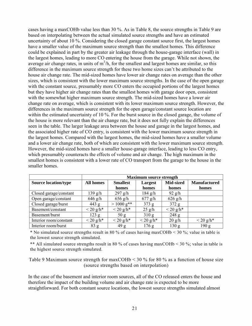
The simulation results constitute a large amount of data as depicted in Figure 8 and Figure 9. One way to interpret these data is to consider the percentage of cases that meet a specific criteria for the target value of maxCOHb. Determination of such criteria is beyond the scope of this project but for comparison purposes Table 8 presents the maximum source strength for which 80 % of the cases simulated are below 30 % maxCOHb for each of the seven source locations and types considered. The values of 80 % below 30 % maxCOHb are used only for illustrative purposes and are not presented as life-safety based limits to support policy or regulatory decisions. Note also that the maximum source strengths in the table are estimated by interpolating between the values used in the simulations. Based on this interpolation, the individual values are estimated to have an uncertainty of approximately 10 %. As noted in the table, none of the simulated source strengths in two of the source locations (Basement/constant and Interior room/constant) resulted in 80 % of the cases being below 30 % maxCOHb. In those cases, the maximum source strength is noted as “< 20 g/h,” noting that 20 g/h was lowest value simulated.

Source location/type Maximum source strength Closed garage/constant 139 g/h Open garage/constant 646 g/h Closed garage/burst 443 g Basement/constant < 20 g/h* Basement/burst 123 g Interior room/constant < 20 g/h* Interior room/burst 83 g

* No simulated source strengths result in 80 % of cases having maxCOHb < 30 %.

Table 8 Maximum source strength corresponding to 80 % of the simulated cases with maxCOHb < 30 % (source strengths based on interpolation between simulated values)

3.4 Summary results for subsets of houses As noted earlier, the simulation results were analyzed separately to examine the impact of house size, airtightness and weather. Separate frequency distributions were generated for the 37 detached homes in the smallest size category, for the 16 in the largest size category and for the remaining 30 “mid-sized” homes, as well as for the four manufactured homes. Separate frequency distributions were also generated for the 20 tightest and 20 leakiest houses, based on their airtightness values from simulated blower door test results in units of air changes per hour at 50 Pa. Finally, the impacts of weather were examined by generating separate frequency distributions of maxCOHb for the two cold weeks of weather, one week of mild weather and one week of warm weather. In interpreting these results it is important to bear in mind the complexity of airflow and contaminant transport in multizone buildings and the fact that these homes differ in more than size and airtightness. Other differences that impact airflow and CO transport include the locations of the garages, the floor plans of the occupied zones in relation to the basement and garage, and other house-specific characteristics. As a result, the differences discussed below are sometimes hard to explain based solely on the size, tightness and weather. Also, the conversion of indoor CO concentrations to %COHb is a nonlinear calculation, which makes the variations in the maximum source strengths for the different cases even more complex. Table 9 presents the maximum source strengths for the different size homes, as well as for the four manufactured homes, with these source strengths again corresponding to 80 % of the simulated

21

cases having a maxCOHb value less than 30 %. As in Table 8, the source strengths in Table 9 are based on interpolating between the actual simulated source strengths and have an estimated uncertainty of about 10 %. Considering the closed garage constant source first, the largest homes have a smaller value of the maximum source strength than the smallest homes. This difference could be explained in part by the greater air leakage through the house-garage interface (wall) in the largest homes, leading to more CO entering the house from the garage. While not shown, the average air change rates, in units of m3/h, for the smallest and largest homes are similar, so this difference in the maximum source strength for these two home sizes can’t be attributed to the house air change rate. The mid-sized homes have lower air change rates on average than the other sizes, which is consistent with the lower maximum source strengths. In the case of the open garage with the constant source, presumably more CO enters the occupied portions of the largest homes but they have higher air change rates than the smallest homes with garage door open, consistent with the somewhat higher maximum source strength. The mid-sized homes have a lower air change rate on average, which is consistent with its lower maximum source strength. However, the differences in the maximum source strength for the open garage/constant source location are within the estimated uncertainty of 10 %. For the burst source in the closed garage, the volume of the house is more relevant than the air change rate, but it does not fully explain the differences seen in the table. The larger leakage area between the house and garage in the largest homes, and the associated higher rate of CO entry, is consistent with the lower maximum source strength in the largest homes. Compared with the largest homes, the mid-sized homes have a smaller volume and a lower air change rate, both of which are consistent with the lower maximum source strength. However, the mid-sized homes have a smaller house-garage interface, leading to less CO entry, which presumably counteracts the effects of volume and air change. The high maximum in the smallest homes is consistent with a lower rate of CO transport from the garage to the house in the smaller homes.

Maximum source strength Source location/type All homes Smallest

homes Largest homes

Mid-sized homes

Manufactured homes

Closed garage/constant 139 g/h 297 g/h 184 g/h 92 g/h Open garage/constant 646 g/h 656 g/h 677 g/h 626 g/h Closed garage/burst 443 g > 1000 g** 373 g 372 g Basement/constant < 20 g/h* < 20 g/h* 25 g/h < 20 g/h* Basement/burst 123 g 50 g 310 g 248 g Interior room/constant < 20 g/h* < 20 g/h* < 20 g/h* 20 g/h < 20 g/h* Interior room/burst 83 g 49 g 176 g 130 g 190 g

* No simulated source strengths result in 80 % of cases having maxCOHb < 30 %; value in table is the lowest source strength simulated. ** All simulated source strengths result in 80 % of cases having maxCOHb < 30 %; value in table is the highest source strength simulated.

Table 9 Maximum source strength for maxCOHb < 30 % for 80 % as a function of house size (source strengths based on interpolation)

In the case of the basement and interior room sources, all of the CO released enters the house and therefore the impact of the building volume and air change rate is expected to be more straightforward. For both constant source locations, the lowest source strengths simulated almost

22

all result in less than 80 % of the cases being below 30 % maxCOHb. The only exception is in the largest homes but the differences are not significant, given the high levels of %COHb calculated for all the source values. The maximum source strengths for the burst sources in the basement and interior room correspond to the house sizes, with the smallest homes having the lowest maximum source strengths and the trend continuing with the mid- and largest size homes. The manufactured homes only have the interior room sources, but the maximum value for the burst source is higher than the detached homes despite the smaller volume of the manufactured homes. The reason for this difference could be related to all the manufactured homes being one story tall, which means that air flowing vertically out of the interior room leaves the occupied spaces. Some of the other homes are two-story, in which upward airflow does not leave the house. Table 10 presents the maximum source strengths corresponding to 80 % of the cases having a maxCOHb value less than 30 % for the twenty tightest and twenty leakiest homes. For all three garage source locations, the leakiest homes have higher maximum sources strengths, which is consistent with their higher air change rates. Similarly, the tightest homes have the lowest maximum source strengths. As noted in the discussion of house size, none of the constant source strengths in the basement or interior room result in 80 % of the cases having a maxCOHb below 30 %. For the burst sources located in the basement and the interior room, the maximum source strength is higher for the tightest homes. This can be explained by the tightest homes having larger volumes than the leakiest homes, since the initial dilution by volume is more important than the dilution over time associated with air change.

Maximum source strength Source location/type All homes Tightest

homes Leakiest homes

Closed garage/constant 139 g/h 76 g/h 820 g/h Open garage/constant 646 g/h 618 g/h 731 g/h Closed garage/burst 443 g 255 g > 1000 g** Basement/constant < 20 g/h* < 20 g/h* < 20 g/h* Basement/burst 123 g 229 g 57 g Interior room/constant < 20 g/h* < 20 g/h* < 20 g/h* Interior room/burst 83 g 143 g 49 g

* No simulated source strengths result in 80 % of cases having maxCOHb < 30 %; value in table is the lowest source strength simulated. ** All simulated source strengths result in 80 % of cases having maxCOHb < 30 %; value in table is the highest source strength simulated.

Table 10 Maximum source strength for maxCOHb < 30 % for 80 % as a function of detached home tightness levels (source strengths based on interpolation)

23

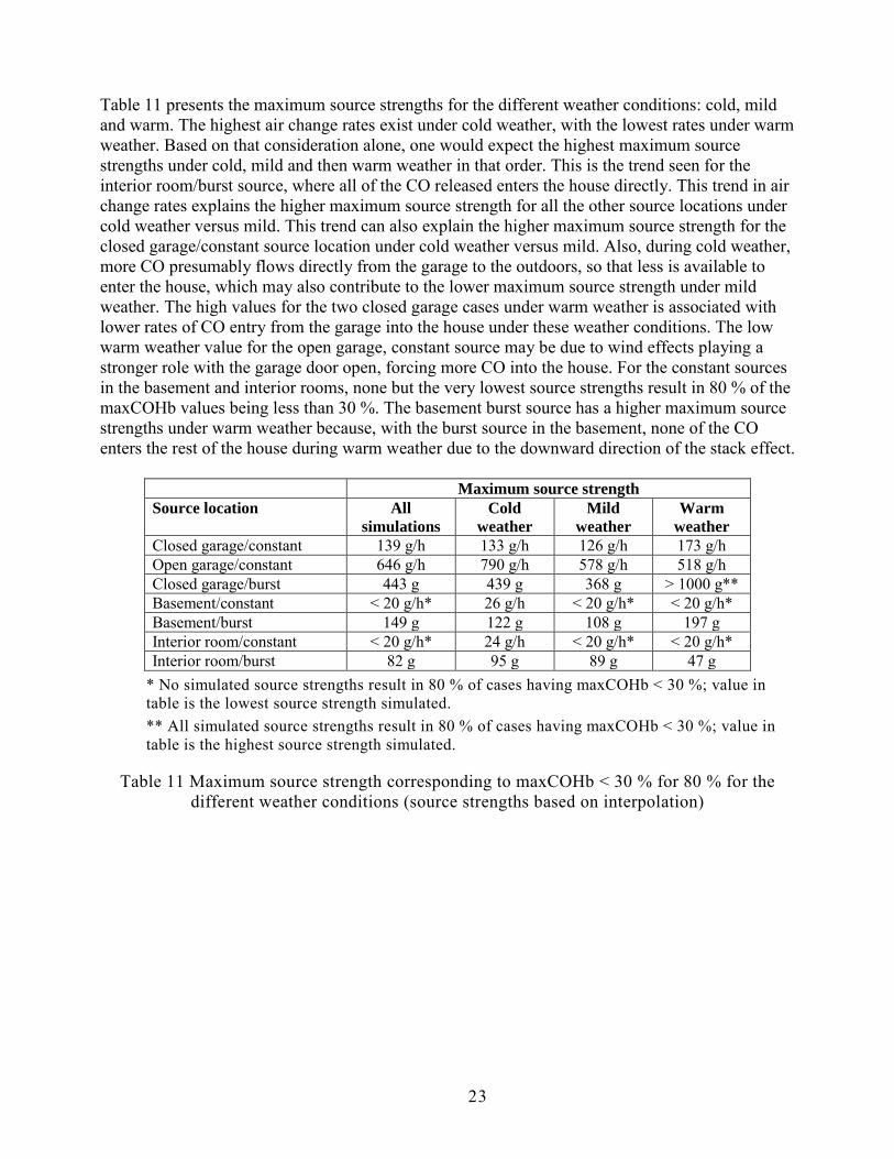
Table 11 presents the maximum source strengths for the different weather conditions: cold, mild and warm. The highest air change rates exist under cold weather, with the lowest rates under warm weather. Based on that consideration alone, one would expect the highest maximum source strengths under cold, mild and then warm weather in that order. This is the trend seen for the interior room/burst source, where all of the CO released enters the house directly. This trend in air change rates explains the higher maximum source strength for all the other source locations under cold weather versus mild. This trend can also explain the higher maximum source strength for the closed garage/constant source location under cold weather versus mild. Also, during cold weather, more CO presumably flows directly from the garage to the outdoors, so that less is available to enter the house, which may also contribute to the lower maximum source strength under mild weather. The high values for the two closed garage cases under warm weather is associated with lower rates of CO entry from the garage into the house under these weather conditions. The low warm weather value for the open garage, constant source may be due to wind effects playing a stronger role with the garage door open, forcing more CO into the house. For the constant sources in the basement and interior rooms, none but the very lowest source strengths result in 80 % of the maxCOHb values being less than 30 %. The basement burst source has a higher maximum source strengths under warm weather because, with the burst source in the basement, none of the CO enters the rest of the house during warm weather due to the downward direction of the stack effect.

Maximum source strength Source location All

simulations Cold

weather Mild

weather Warm

weather Closed garage/constant 139 g/h 133 g/h 126 g/h 173 g/h Open garage/constant 646 g/h 790 g/h 578 g/h 518 g/h Closed garage/burst 443 g 439 g 368 g > 1000 g** Basement/constant < 20 g/h* 26 g/h < 20 g/h* < 20 g/h* Basement/burst 149 g 122 g 108 g 197 g Interior room/constant < 20 g/h* 24 g/h < 20 g/h* < 20 g/h* Interior room/burst 82 g 95 g 89 g 47 g

* No simulated source strengths result in 80 % of cases having maxCOHb < 30 %; value in table is the lowest source strength simulated. ** All simulated source strengths result in 80 % of cases having maxCOHb < 30 %; value in table is the highest source strength simulated.

Table 11 Maximum source strength corresponding to maxCOHb < 30 % for 80 % for the different weather conditions (source strengths based on interpolation)

24

4. SUMMARY AND DISCUSSION This simulation study was conducted to evaluate indoor CO exposures as a function of generator source location and CO emission rate in order to support life-safety based analyses of potential CO emission limits for generators. These simulations employed the multizone airflow and contaminant transport model CONTAM, which was applied to 87 single-family, detached dwellings that are representative of the U.S. housing stock for that housing type. A total of almost one-hundred thousand individual 24-hour simulations were conducted that cover a range of house layouts and sizes, airtightness levels and weather conditions, as well as generator locations and CO source strengths. The locations include attached garages and basements, in the houses that have such spaces, and a first floor interior room in all of the houses considered. This report presents the simulation results in terms of the maximum levels of percent COHb for the occupied portions of the dwellings as a function of CO emission rate for each indoor source location. It is important to note that the simulation results presented in this report demonstrate the complexity of multizone airflow and contaminant transport in buildings, which in turn supports the value in considering a wide range of homes and weather conditions in addressing the objective of this study. Variations in house layout, source location, outdoor temperature and wind speed and direction can all have significant, and at times complex, impacts on airflow and CO transport. This inherent variability means that considering only one or a small number of buildings under a limited range of conditions may not be adequate to fully understand the levels of CO exposure in residences as a function of generator location and CO emission rate. While the analysis of the subsets of cases based on house size, tightness and weather conditions provide interesting insights, the difficulty in interpreting some of the results highlights the complexity of the problem. The results of the simulations are summarized as frequency distributions of these maxCOHb levels in the occupied zones of the simulated homes. Frequency distributions are presented for all the simulations, as well as for subsets of the simulations based on different size houses, airtightness levels and weather conditions. To support interpretation of these data, each frequency distribution is characterized by the maximum source strength for which 80 % of the cases are below 30 % maxCOHb. These two values are used only for illustrative purposes and are not presented as life-safety based limits to support policy or regulatory decisions. Figure 10 is the frequency distribution of the maxCOHb values for all of the constant source cases, i.e. a generator operating for 18 hours. Considering all the constant source results, the maximum source strength corresponding to 80 % of the cases having a value of maxCOHb below 30 % is 27 g/h. This value is on the low end of those simulated, which indicates that operating a generator for 18 hours as simulated in this study is likely to result in high CO exposures whether the generator is in the house or the garage. Note that the CO emission rates measured in unmodified generators in a separate NIST study tended to be above this value [2].

25

Figure 10 Frequency Distribution of %COHb for All Constant Sources

Figure 11 is the frequency distribution of the maxCOHb values for all of the burst source cases. Considering all of the burst results, the maximum source strength corresponding to 80 % of the cases having a value of maxCOHb below 30 % is 139 g. This value is on the higher end of the burst source strengths measured by NIST (as indicated in Table 4), i.e., there were many measurements below this value in the modified generators. Therefore, generators that are modified to limit CO emissions using an effective shut off or other technology have the potential to significantly reduce indoor CO exposures relative to continuously operating generators with no such emissions controls.

Figure 11 Frequency Distribution of %COHb for All Burst Sources

26

5. ACKNOWLEDGEMENTS This work was funded by the U.S. Consumer Products Safety Commission under interagency agreement No. CPSC-I-09-0017. The authors wish to express their appreciation for the support of Janet Buyer, Sandra Inkster, Han Lim and Donald Switzer in conducting this effort. 6. REFERENCES 1. Hnatov, M.V. 2012. Incidents, Deaths, and In-Depth Investigations Associated with Non-

Fire Carbon Monoxide from Engine-Driven Generators and Other Engine-Driven Tools, 1999-2011. U.S. Consumer Product Safety Commission.

2. Emmerich, S.J., A.K. Persily, and L. Wang. 2013. Modeling and Measuring the Effects of Portable Gasoline Powered Generator Exhaust on Indoor Carbon Monoxide Level. Technical Note 1781. National Institute of Standards and Technology.

3. Walton, G.N. and W.S. Dols. 2005. CONTAMW 2.4 User Guide and Program Documentation. NISTIR 7251. National Institute of Standards and Technology.

4. Persily, A.K., A. Musser, and D. Leber. 2006. A Collection of Homes to Represent the U.S. Housing Stock. NISTIR 7330. National Institute of Standards and Technology.

5. HUD. 1999. American Housing Survey for the United States. U.S. Department of Housing and Urban Development, U.S. Department of Commerce.

6. DOE. Residential Energy Consumption Survey (RECS). 2005; Available from: http://www.eia.doe.gov/emeu/recs/contents.html.

7. Sherman, M. and D. Dickeroff, Air-Tightness of U.S. Dwellings. ASHRAE Transactions, 1998. 104 (2): p. 1359-1367.

8. Chan, W., P. Price, W. Nazaroff, and A. Gadgil, Distribution of Residential Air Leakage: Implications for Health Outcome of an Outdoor Toxic Release. Indoor Air, 2005. 15 (11): p. 1729-1734.

9. Chan, W., P. Price, M. Sohn, and A. Gadgil. 2003. Analysis of U.S. Residential Air Leakage Database. LBNL-53367. Lawrence Berkeley National Laboratory.

10. ASHRAE, Fundamentals Handbook. 2009, Atlanta, GA: American Society of Heating, Refrigerating and Air-Conditioning Engineers, Inc.

11. Emmerich, S.J., Validation of Multizone IAQ Modeling of Residential-Scale Buildings: A Review. ASHRAE Transactions, 2001. 107 (2): p. 619-628.

12. Emmerich, S.J., C. Howard-Reed, and S.J. Nabinger, Validation of multizone IAQ model predictions for tracer gas in a townhouse. Building Service Engineering Research Technology, 2004. 25(4): p. 305-316.

13. Wang, L., S.J. Emmerich, and A.K. Persily, In situ Experimental Study of Carbon Monoxide Generation 1 by Gasoline-Powered Electric Generator in an Enclosed Space. 2010. 60: p. 1443-1451.

27

14. Inkster, S.E. 2006. An estimation of how reductions in the carbon monoxide (C0)'emission rate of portable, gasoline-powered generators could impact the chance of surviving an acute CO exposure resulting from operation of a portable gasoline-powered generator in a basement. U.S. Consumer Product Safety Commission.

15. Peterson, J.E. and R.D. Stewart, Predicting the carboxyhemoglobin levels resulting from carbon monoxide exposures. Journal of Applied Physiology, 1975. 39 (4): p. 633-638.

16. Coburn, R.F., R.E. Forster, and P.B. Kane, Considerations of the physiological variables that determine the blood carboxyhemoglobin concentration in man. Journal of Clinical Investigation, 1965. 44 (11): p. 1899-1910.

17. Goldstein, M., Carbon Monoxide Poisoning. Journal of Emergency Nursing, 2008. 34(6): p. 538-542.

28

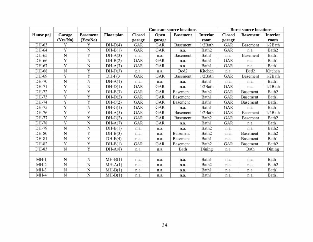
APPENDIX A: House Characteristics This appendix contains two tables that define the 87 dwellings, with one table for each housing type: detached (A1) and manufactured home (A2). The dwelling definitions in the table are in terms of the variables discussed in detail in the report that defines these homes [4]. Table A1. Detached Homes (83 total) Key for Table A1: # of floors: 1 = one story; 2 = two story Floor area: 1 = less than 148.5 m2 (1,599 ft2); 2 = 148.6 m2

to 222.9 m2 (1,600 ft2 to 2,399 ft2); 3 = 223.0 m2

(2,400 ft2) or more Year Built: 1 = before 1940; 2 = 1940-69; 3 = 1970-89; 4 = 1990 and newer Foundation: 1 = concrete slab; 2 = crawl space; 3 = finished basement, 4 = unfinished basement Garage: 1 = none; 2 = attached garage Forced Air: 1 = other; 2 = central system present

House Number # of Floors

House Variable # of Rooms

Floor plan Floor area Year Built Foundation Garage Forced -air Bed-rooms Full baths Half baths Other

DH-1 1 2 3 1 2 2 3 2 0 3 DH-B(1) DH-2 1 1 2 3 2 2 3 1 0 3 DH-A(8) DH-3 1 1 2 2 1 1 2 1 0 2 DH-A(1) DH-4 1 1 2 2 2 2 3 1 0 3 DH-A(7) DH-5 1 1 3 1 2 2 3 2 0 3 DH-A(2) DH-6 2 1 1 3 2 2 3 1 0 3 DH-D(3) DH-7 1 2 2 3 2 2 3 2 0 4 DH-B(5) DH-8 1 1 2 1 2 2 3 2 0 3 DH-A(2) DH-9 2 1 2 3 2 2 3 1 0 3 DH-D(3)

DH-10 2 2 3 3 2 2 4 2 1 4 DH-E(8) DH-11 1 1 2 2 2 1 3 1 0 3 DH-A(7) DH-12 2 3 3 3 2 2 4 2 1 5 DH-F(4) DH-13 1 2 2 2 2 2 3 2 0 3 DH-B(1) DH-14 2 2 1 3 2 2 3 1 1 4 DH-E(5) DH-15 2 3 4 3 2 2 4 3 1 5 DH-F(5)

29

House Number # of Floors

House Variable # of Rooms

Floor plan Floor area Year Built Foundation Garage Forced -air Bed-rooms Full baths Half baths Other

DH-16 1 1 2 2 1 2 3 1 0 3 DH-A(7) DH-17 2 2 2 3 2 2 3 2 1 4 DH-E(6) DH-18 2 1 1 3 1 2 3 1 0 3 DH-D(3) DH-19 1 1 3 3 2 2 3 1 0 3 DH-A(8) DH-20 2 2 1 3 2 1 4 1 0 4 DH-E(7) DH-21 1 1 2 1 1 2 3 1 0 3 DH-A(7) DH-22 2 3 3 1 2 2 4 3 1 5 DH-F(1) DH-23 2 1 1 3 2 1 3 1 0 3 DH-D(3) DH-24 2 2 3 1 2 2 4 2 1 4 DH-E(3) DH-25 1 1 2 3 2 1 3 1 0 3 DH-A(8) DH-26 1 1 2 1 1 1 2 1 0 2 DH-A(1) DH-27 1 1 2 3 1 2 3 1 0 3 DH-A(8) DH-28 2 3 4 1 2 2 4 3 1 4 DH-F(2) DH-29 1 1 1 2 1 1 2 1 0 3 DH-A(3) DH-30 1 2 3 2 2 2 3 2 0 3 DH-B(1) DH-31 1 1 3 2 2 2 3 2 0 3 DH-A(2) DH-32 1 1 4 1 2 2 3 2 0 2 DH-A(6) DH-33 1 3 3 1 2 2 4 2 0 4 DH-C(1) DH-34 1 1 3 1 1 2 3 1 0 3 DH-A(7) DH-35 1 2 2 1 2 2 3 2 0 3 DH-B(1) DH-36 2 2 4 1 2 2 4 2 1 4 DH-E(3) DH-37 1 2 3 3 2 2 3 2 1 3 DH-B(4) DH-38 1 1 3 2 1 2 3 1 0 3 DH-A(7) DH-39 1 2 2 2 1 2 3 2 0 3 DH-B(1) DH-40 2 2 3 2 2 2 4 2 1 4 DH-E(3) DH-41 2 2 1 3 1 2 3 1 0 4 DH-E(1) DH-42 1 1 3 2 1 1 3 1 0 2 DH-A(4) DH-43 2 2 2 3 2 1 4 2 0 4 DH-E(2) DH-44 1 1 1 3 2 2 2 1 0 3 DH-A(9) DH-45 2 2 3 4 2 1 4 2 1 4 DH-E(3) DH-46 1 1 2 1 2 1 2 1 0 2 DH-A(1) DH-47 1 1 3 2 2 1 3 1 0 3 DH-A(7)

30

House Number # of Floors

House Variable # of Rooms

Floor plan Floor area Year Built Foundation Garage Forced -air Bed-rooms Full baths Half baths Other

DH-48 1 1 4 2 1 2 3 2 0 3 DH-A(2) DH-49 1 1 2 3 1 1 3 1 0 3 DH-A(8) DH-50 2 1 1 3 1 1 3 1 0 3 DH-D(3) DH-51 2 3 3 2 2 2 4 2 1 4 DH-F(3) DH-52 2 3 1 4 2 2 4 2 1 4 DH-F(3) DH-53 1 2 3 1 1 2 3 2 0 3 DH-B(1) DH-54 1 1 1 2 1 2 2 1 0 3 DH-A(3) DH-55 1 1 4 2 2 2 3 2 0 2 DH-A(6) DH-56 2 1 2 3 1 2 3 1 0 3 DH-D(3) DH-57 1 2 2 2 2 1 3 2 0 4 DH-B(3) DH-58 2 2 4 3 2 2 3 2 1 4 DH-E(6) DH-59 2 3 2 3 2 1 4 2 1 5 DH-F(4) DH-60 1 1 3 4 2 1 3 1 0 3 DH-A(7) DH-61 1 1 1 4 1 2 2 1 0 2 DH-A(1) DH-62 2 3 1 3 2 1 4 2 1 5 DH-F(4) DH-63 2 1 2 4 2 1 3 1 1 3 DH-D(4) DH-64 1 2 4 1 2 2 3 2 0 3 DH-B(1) DH-65 1 1 1 4 1 1 2 1 0 3 DH-A(3) DH-66 1 2 2 1 2 1 3 1 0 3 DH-B(2) DH-67 1 1 1 2 2 2 3 1 0 3 DH-A(7) DH-68 2 1 2 3 1 1 3 1 0 3 DH-D(3) DH-69 2 3 3 4 2 1 4 2 1 4 DH-F(3) DH-70 1 1 3 1 1 1 2 1 0 2 DH-A(1) DH-71 2 1 3 1 2 2 3 2 1 3 DH-D(1) DH-72 1 2 1 4 2 2 3 2 0 4 DH-B(3) DH-73 2 1 3 4 2 2 3 2 0 4 DH-D(2) DH-74 1 3 3 4 2 2 3 2 1 5 DH-C(2) DH-75 3 2 3 1 2 2 4 2 1 3 DH-G(1) DH-76 1 1 4 4 2 2 3 2 1 3 DH-A(5) DH-77 3 2 3 4 2 2 3 2 1 4 DH-G(2) DH-78 1 1 3 1 2 1 3 1 0 3 DH-A(7) DH-79 1 2 3 2 1 2 3 2 0 3 DH-B(1)

31

House Number # of Floors

House Variable # of Rooms

Floor plan Floor area Year Built Foundation Garage Forced -air Bed-rooms Full baths Half baths Other

DH-80 1 2 2 4 1 2 3 2 0 4 DH-B(3) DH-81 2 2 1 4 1 1 3 2 0 4 DH-E(4) DH-82 1 2 2 4 2 1 3 2 0 3 DH-B(1) DH-83 1 1 3 3 1 2 3 1 0 3 DH-A(8)

TABLE A2. Manufactured Homes Key for Table A2: Floor area: 1 = less than 148.5 m2

(1,599 ft2); 2 = 148.6 m2 (1,600 ft2) or more

Year Built: 1 = before 1940; 2 = 1940-69; 3 = 1970-89; 4 = 1990 and newer Forced Air: 1 = other; 2 = central system present

House Number

Floor area

Year Built

Forced-air

# of Bedrooms

# of Baths

# of Half baths

# of Other rooms Floor plan

MH-1 1 3 2 2 1 0 2 MH-B(1) MH-2 1 4 2 3 2 0 2 MH-A(1) MH-3 1 3 1 2 1 0 2 MH-B(1) MH-4 1 2 2 2 1 0 2 MH-B(1)

32

Appendix B Source Locations for Each House

House prj

Constant source locations Burst source locations Garage

(Yes/No) Basement (Yes/No)

Floor plan Closed garage

Open garage

Basement Interior room

Closed garage

Basement Interior room

DH-1 Y N DH-B(1) GAR GAR n.a. Bath2 GAR n.a. Bath2 DH-2 Y Y DH-A(8) GAR GAR Bath1 Dining GAR Bath1 Dining DH-3 N N DH-A(1) n.a. n.a. n.a. Bath1 n.a. n.a. Bath1 DH-4 Y N DH-A(7) GAR GAR n.a. Bath1 GAR n.a. Bath1 DH-5 Y N DH-A(2) GAR GAR n.a. Bath2 GAR n.a. Bath2 DH-6 Y Y DH-D(3) GAR GAR Bed2 Kitchen GAR Bed2 Kitchen DH-7 Y Y DH-B(5) GAR GAR Den Bath1 GAR Den Bath1 DH-8 Y N DH-A(2) GAR GAR n.a. Bath2 GAR n.a. Bath2 DH-9 Y Y DH-D(3) GAR GAR Bed2 Kitchen GAR Bed2 Kitchen

DH-10 Y Y DH-E(8) GAR GAR Bath2 1/2Bath GAR Bath2 1/2Bath DH-11 Y N DH-A(7) GAR GAR n.a. Bath1 GAR n.a. Bath1 DH-12 Y Y DH-F(4) GAR GAR Bath2 1/2Bath GAR Bath2 1/2Bath DH-13 Y N DH-B(1) GAR GAR n.a. Bath2 GAR n.a. Bath2 DH-14 Y Y DH-E(5) GAR GAR Den 1/2Bath GAR Den 1/2Bath DH-15 Y Y DH-F(5) GAR GAR Bath3 1/2Bath GAR Bath3 1/2Bath DH-16 N N DH-A(7) n.a. n.a. n.a. Bath1 n.a. n.a. Bath1 DH-17 Y Y DH-E(6) GAR GAR Bath2 1/2Bath GAR Bath2 1/2Bath DH-18 N Y DH-D(3) n.a. n.a. Bed2 Kitchen n.a. Bed2 Kitchen DH-19 Y Y DH-A(8) GAR GAR Bath Dining GAR Bath Dining DH-20 Y Y DH-E(7) GAR GAR Den Dining GAR Den Dining DH-21 N N DH-A(7) n.a. n.a. n.a. Bath1 n.a. n.a. Bath1 DH-22 Y N DH-F(1) GAR GAR n.a. 1/2Bath GAR n.a. 1/2Bath DH-23 Y Y DH-D(3) GAR GAR Bed2 Kitchen GAR Bed2 Kitchen DH-24 Y N DH-E(3) GAR GAR n.a. 1/2Bath GAR n.a. 1/2Bath DH-25 Y Y DH-A(8) GAR GAR Bath Dining GAR Bath Dining DH-26 N N DH-A(1) n.a. n.a. n.a. Bath1 n.a. n.a. Bath1 DH-27 N Y DH-A(8) n.a. n.a. Bath Dining n.a. Bath Dining DH-28 Y N DH-F(2) GAR GAR n.a. 1/2Bath GAR n.a. 1/2Bath DH-29 N N DH-A(3) n.a. n.a. n.a. Bath1 n.a. n.a. Bath1 DH-30 Y N DH-B(1) GAR GAR n.a. Bath2 GAR n.a. Bath2

33

House prj

Constant source locations Burst source locations Garage

(Yes/No) Basement (Yes/No)

Floor plan Closed garage

Open garage

Basement Interior room

Closed garage

Basement Interior room

DH-31 Y N DH-A(2) GAR GAR n.a. Bath2 GAR n.a. Bath2 DH-32 Y N DH-A(6) GAR GAR n.a. Bath2 GAR n.a. Bath2 DH-33 Y N DH-C(1) GAR GAR n.a. Bath2 GAR n.a. Bath2 DH-34 N N DH-A(7) n.a. n.a. n.a. Bath1 n.a. n.a. Bath1 DH-35 Y N DH-B(1) GAR GAR n.a. Bath2 GAR n.a. Bath2 DH-36 Y N DH-E(3) GAR GAR n.a. 1/2Bath GAR n.a. 1/2Bath DH-37 Y Y DH-B(4) GAR GAR Bath1 1/2Bath GAR Bath1 1/2Bath DH-38 N N DH-A(7) n.a. n.a. n.a. Bath1 n.a. n.a. Bath1 DH-39 N N DH-B(1) n.a. n.a. n.a. Bath2 n.a. n.a. Bath2 DH-40 Y N DH-E(3) GAR GAR n.a. 1/2Bath GAR n.a. 1/2Bath DH-41 N Y DH-E(1) n.a. n.a. Den Dining n.a. Den Dining DH-42 N N DH-A(4) n.a. n.a. n.a. Bath1 n.a. n.a. Bath1 DH-43 Y Y DH-E(2) GAR GAR Bath2 Dining GAR Bath2 Dining DH-44 Y Y DH-A(9) GAR GAR Bath Dining GAR Bath Dining DH-45 Y Y DH-E(3) GAR GAR Basement Bath1 GAR Basement Bath1 DH-46 Y N DH-A(1) GAR GAR n.a. Bath1 GAR n.a. Bath1 DH-47 Y N DH-A(7) GAR GAR n.a. Bath1 GAR n.a. Bath1 DH-48 N N DH-A(2) n.a. n.a. n.a. Bath2 n.a. n.a. Bath2 DH-49 N Y DH-A(8) n.a. n.a. Bath Dining n.a. Bath Dining DH-50 N Y DH-D(3) n.a. n.a. Bed2 Kitchen n.a. Bed2 Kitchen DH-51 Y N DH-F(3) GAR GAR n.a. 1/2Bath GAR n.a. 1/2Bath DH-52 Y Y DH-F(3) GAR GAR Basement 1/2Bath GAR Basement 1/2Bath DH-53 N N DH-B(1) n.a. n.a. n.a. Bath2 n.a. n.a. Bath2 DH-54 N N DH-A(3) n.a. n.a. n.a. Bath1 n.a. n.a. Bath1 DH-55 Y N DH-A(6) GAR GAR n.a. Bath2 GAR n.a. Bath2 DH-56 N Y DH-D(3) n.a. n.a. Bed2 Kitchen n.a. Bed2 Kitchen DH-57 Y N DH-B(3) GAR GAR n.a. Bath2 GAR n.a. Bath2 DH-58 Y Y DH-E(6) GAR GAR Bath2 1/2Bath GAR Bath2 1/2Bath DH-59 Y Y DH-F(4) GAR GAR Bath2 1/2Bath GAR Bath2 1/2Bath DH-60 Y Y DH-A(7) GAR GAR Basement Bath1 GAR Basement Bath1 DH-61 N Y DH-A(1) n.a. n.a. Basement Bath1 n.a. Basement Bath1 DH-62 Y Y DH-F(4) GAR GAR Bath2 1/2Bath GAR Bath2 1/2Bath

34

House prj

Constant source locations Burst source locations Garage

(Yes/No) Basement (Yes/No)

Floor plan Closed garage

Open garage

Basement Interior room

Closed garage

Basement Interior room

DH-63 Y Y DH-D(4) GAR GAR Basement 1/2Bath GAR Basement 1/2Bath DH-64 Y N DH-B(1) GAR GAR n.a. Bath2 GAR n.a. Bath2 DH-65 N Y DH-A(3) n.a. n.a. Basement Bath1 n.a. Basement Bath1 DH-66 Y N DH-B(2) GAR GAR n.a. Bath1 GAR n.a. Bath1 DH-67 Y N DH-A(7) GAR GAR n.a. Bath1 GAR n.a. Bath1 DH-68 N Y DH-D(3) n.a. n.a. Bed2 Kitchen n.a. Bed2 Kitchen DH-69 Y Y DH-F(3) GAR GAR Basement 1/2Bath GAR Basement 1/2Bath DH-70 N N DH-A(1) n.a. n.a. n.a. Bath1 n.a. n.a. Bath1 DH-71 Y N DH-D(1) GAR GAR n.a. 1/2Bath GAR n.a. 1/2Bath DH-72 Y Y DH-B(3) GAR GAR Basement Bath2 GAR Basement Bath2 DH-73 Y Y DH-D(2) GAR GAR Basement Bath1 GAR Basement Bath1 DH-74 Y Y DH-C(2) GAR GAR Basement Bath1 GAR Basement Bath1 DH-75 Y N DH-G(1) GAR GAR n.a. Bath1 GAR n.a. Bath1 DH-76 Y Y DH-A(5) GAR GAR Basement 1/2Bath GAR Basement 1/2Bath DH-77 Y Y DH-G(2) GAR GAR Basement Bath2 GAR Basement Bath2 DH-78 Y N DH-A(7) GAR GAR n.a. Bath1 GAR n.a. Bath1 DH-79 N N DH-B(1) n.a. n.a. n.a. Bath2 n.a. n.a. Bath2 DH-80 N Y DH-B(3) n.a. n.a. Basement Bath2 n.a. Basement Bath2 DH-81 N Y DH-E(4) n.a. n.a. Basement Bath1 n.a. Basement Bath1 DH-82 Y Y DH-B(1) GAR GAR Basement Bath2 GAR Basement Bath2 DH-83 N Y DH-A(8) n.a. n.a. Bath Dining n.a. Bath Dining

MH-1 N N MH-B(1) n.a. n.a. n.a. Bath1 n.a. n.a. Bath1 MH-2 N N MH-A(1) n.a. n.a. n.a. Bath2 n.a. n.a. Bath2 MH-3 N N MH-B(1) n.a. n.a. n.a. Bath1 n.a. n.a. Bath1 MH-4 N N MH-B(1) n.a. n.a. n.a. Bath1 n.a. n.a. Bath1

35

Appendix C Integral Mass Balance Analysis of Burst Sources The following method was used to estimate the total CO mass released during a test in which the generator runs for a relatively short period of time (minutes), so-called burst sources. This analysis approach applies to a generator with a shutoff mechanism or some other technology that results in a generation rate that can’t be well characterized with a constant source strength. As described below, it was used to estimate the burst source strengths that were employed in the analysis described in the body of this report and which are listed in Table 4. This analysis method was applied to a series of generator tests conducted in the NIST test house, with the generator in the garage, as described in reference [2]. The mass balance of CO in a single-zone (i.e., the NIST test house garage) can be expressed as:

where

V = zone volume, m3 C = CO concentration in zone, mg/m3 Cout = CO concentration in outdoors, mg/m3 t = time, min Q = airflow rate through zone, m3/min S = CO generation rate, mg/min

Also, T is the length of time (min) over which CO is emitted by the generator. Assuming that Cout = 0 and taking the integral of both sides of the equation from t1 to t2 yields:

,

which can be expressed as:

where = average generation rate over the time interval during which CO is released

C2 = C at time t2 C1 = C at time t1

is the total mass of CO released over the period of interest and is the quantity that is being

estimated with this analysis approach. In applying this approach to the garage tests conducted in the NIST test house, Q can be estimated from the decay in the concentration of CO after the generator stops operating for cases in which

VdCdt

= QCout − QC + S(t)

V dC = −Qt1

t2

∫ Cdtt1

t2

∫ + Sdtt1

t2

∫

S T = V (C2 − C1) + Q Cdtt1

t2

∫

S

S T

36

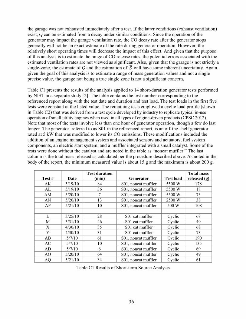
the garage was not exhausted immediately after a test. If the latter conditions (exhaust ventilation) exist, Q can be estimated from a decay under similar conditions. Since the operation of the generator may impact the garage ventilation rate, the CO decay rate after the generator stops generally will not be an exact estimate of the rate during generator operation. However, the relatively short operating times will decrease the impact of this effect. And given that the purpose of this analysis is to estimate the range of CO release rates, the potential errors associated with the estimated ventilation rates are not viewed as significant. Also, given that the garage is not strictly a single-zone, the estimate of Q and the estimation of will have some inherent uncertainty. Again, given the goal of this analysis is to estimate a range of mass generation values and not a single precise value, the garage not being a true single zone is not a significant concern. Table C1 presents the results of the analysis applied to 14 short-duration generator tests performed by NIST in a separate study [2]. The table contains the test number corresponding to the referenced report along with the test date and duration and test load. The test loads in the first five tests were constant at the listed value. The remaining tests employed a cyclic load profile (shown in Table C2) that was derived from a test cycle developed by industry to replicate typical in-use operation of small utility engines when used in all types of engine-driven products (CPSC 2012). Note that most of the tests involve less than one hour of generator operation, though a few do last longer. The generator, referred to as S01 in the referenced report, is an off-the-shelf generator rated at 5 kW that was modified to lower its CO emissions. These modifications included the addition of an engine management system and associated sensors and actuators, fuel system components, an electric start system, and a muffler integrated with a small catalyst. Some of the tests were done without the catalyst and are noted in the table as “noncat muffler.” The last column is the total mass released as calculated per the procedure described above. As noted in the body of the report, the minimum measured value is about 15 g and the maximum is about 200 g.

Test # Date Test duration

(min) Generator Test load Total mass released (g)

AK 5/19/10 84 S01, noncat muffler 5500 W 178 AL 5/19/10 36 S01, noncat muffler 5500 W 18 AM 5/20/10 7 S01, noncat muffler 5500 W 73 AN 5/20/10 13 S01, noncat muffler 2500 W 38 AP 5/21/10 10 S01, noncat muffler 500 W 108

L 3/25/10 28 S01 cat muffler Cyclic 68 M 3/31/10 46 S01 cat muffler Cyclic 49 X 4/30/10 35 S01 cat muffler Cyclic 68 Y 4/30/10 31 S01 cat muffler Cyclic 73

AB 5/7/10 61 S01, noncat muffler Cyclic 190 AC 5/7/10 10 S01, noncat muffler Cyclic 135 AD 5/7/10 6 S01, noncat muffler Cyclic 69 AO 5/20/10 64 S01, noncat muffler Cyclic 49 AQ 5/21/10 34 S01, noncat muffler Cyclic 61

Table C1 Results of Short-term Source Analysis

S

37

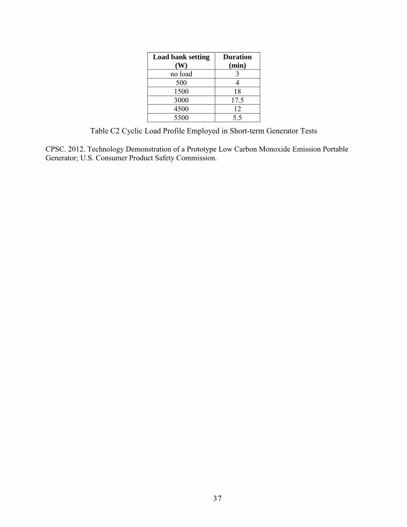
Load bank setting

(W) Duration

(min) no load 3

500 4 1500 18 3000 17.5 4500 12 5500 5.5

Table C2 Cyclic Load Profile Employed in Short-term Generator Tests CPSC. 2012. Technology Demonstration of a Prototype Low Carbon Monoxide Emission Portable Generator; U.S. Consumer Product Safety Commission.

38

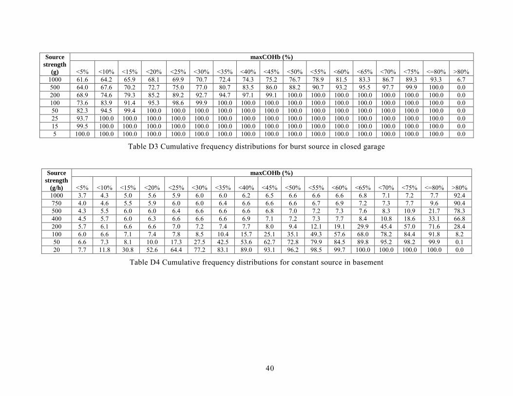
Appendix D Cumulative Frequency Distributions of maxCOHb in Tabular Form This appendix presents the cumulative frequency distributions for all source locations in the tabular format used in Table 7. The data for the constant source in the interior room, presented in those figures and tables, is repeated here for completeness. Note again that the last column in each table is the percentage of cases above 80 % COHb, which is not typically the way in which cumulative distributions are presented but is more meaningful in this case. The tables contained in this appendix are as follows: Table D1 Cumulative frequency distributions for constant source in closed garage Table D2 Cumulative frequency distributions for constant source in open garage Table D3 Cumulative frequency distributions for burst source in closed garage Table D4 Cumulative frequency distributions for constant source in basement

Table D5 Cumulative frequency distributions for burst source in basement Table D6 Cumulative frequency distributions for constant source in interior room Table D7 Cumulative frequency distributions for burst source in interior room

39

Source strength

(g/h)

maxCOHb (%)

<5% <10% <15% <20% <25% <30% <35% <40% <45% <50% <55% <60% <65% <70% <75% <=80% >80% 1000 2.4 5.7 12.7 19.7 28.1 34.2 40.0 47.3 51.2 54.1 57.5 62.3 66.1 70.4 77.3 83.8 16.2 750 3.1 10.1 18.1 28.2 35.5 43.3 49.5 52.8 56.1 60.2 64.2 67.5 72.4 78.3 83.9 89.0 11.0 500 5.2 17.3 30.6 39.1 48.4 52.9 56.4 61.3 64.8 68.1 72.6 78.0 82.6 86.4 91.2 95.9 4.1 400 8.3 23.8 36.1 47.5 52.8 56.7 61.7 65.5 69.1 73.9 78.4 82.9 86.3 90.9 95.0 99.3 0.7 200 21.7 44.4 54.1 60.8 66.2 70.9 76.8 80.8 84.9 87.9 91.9 95.1 98.6 99.4 99.5 99.8 0.3 100 42.4 58.8 68.1 75.7 81.6 85.7 90.4 93.4 96.7 99.3 99.4 99.5 99.7 99.8 99.9 100.0 0.0 50 57.6 72.8 83.2 88.9 93.6 97.9 99.4 99.4 99.6 99.8 99.8 99.9 100.0 100.0 100.0 100.0 0.0 20 77.7 91.7 98.7 99.4 99.8 99.8 99.9 100.0 100.0 100.0 100.0 100.0 100.0 100.0 100.0 100.0 0.0

Table D1 Cumulative frequency distributions for constant source in closed garage

Source strength

(g/h)

maxCOHb (%)

<5% <10% <15% <20% <25% <30% <35% <40% <45% <50% <55% <60% <65% <70% <75% <=80% >80% 1000 2.4 2.8 4.0 5.5 8.5 18.2 58.0 84.5 94.3 98.1 99.8 100.0 100.0 100.0 100.0 100.0 0.0 750 2.7 3.5 5.2 9.0 22.7 68.9 90.7 95.8 99.6 100.0 100.0 100.0 100.0 100.0 100.0 100.0 0.0 500 2.8 5.0 10.4 45.4 86.8 95.5 99.5 100.0 100.0 100.0 100.0 100.0 100.0 100.0 100.0 100.0 0.0 400 3.1 6.5 24.7 81.7 95.3 99.5 100.0 100.0 100.0 100.0 100.0 100.0 100.0 100.0 100.0 100.0 0.0 200 6.0 69.7 96.8 100.0 100.0 100.0 100.0 100.0 100.0 100.0 100.0 100.0 100.0 100.0 100.0 100.0 0.0 100 57.5 99.8 100.0 100.0 100.0 100.0 100.0 100.0 100.0 100.0 100.0 100.0 100.0 100.0 100.0 100.0 0.0 50 99.6 100.0 100.0 100.0 100.0 100.0 100.0 100.0 100.0 100.0 100.0 100.0 100.0 100.0 100.0 100.0 0.0 20 100.0 100.0 100.0 100.0 100.0 100.0 100.0 100.0 100.0 100.0 100.0 100.0 100.0 100.0 100.0 100.0 0.0

Table D2 Cumulative frequency distributions for constant source in open garage

40

Source

strength (g)

maxCOHb (%)

<5% <10% <15% <20% <25% <30% <35% <40% <45% <50% <55% <60% <65% <70% <75% <=80% >80% 1000 61.6 64.2 65.9 68.1 69.9 70.7 72.4 74.3 75.2 76.7 78.9 81.5 83.3 86.7 89.3 93.3 6.7 500 64.0 67.6 70.2 72.7 75.0 77.0 80.7 83.5 86.0 88.2 90.7 93.2 95.5 97.7 99.9 100.0 0.0 200 68.9 74.6 79.3 85.2 89.2 92.7 94.7 97.1 99.1 100.0 100.0 100.0 100.0 100.0 100.0 100.0 0.0 100 73.6 83.9 91.4 95.3 98.6 99.9 100.0 100.0 100.0 100.0 100.0 100.0 100.0 100.0 100.0 100.0 0.0 50 82.3 94.5 99.4 100.0 100.0 100.0 100.0 100.0 100.0 100.0 100.0 100.0 100.0 100.0 100.0 100.0 0.0 25 93.7 100.0 100.0 100.0 100.0 100.0 100.0 100.0 100.0 100.0 100.0 100.0 100.0 100.0 100.0 100.0 0.0 15 99.5 100.0 100.0 100.0 100.0 100.0 100.0 100.0 100.0 100.0 100.0 100.0 100.0 100.0 100.0 100.0 0.0 5 100.0 100.0 100.0 100.0 100.0 100.0 100.0 100.0 100.0 100.0 100.0 100.0 100.0 100.0 100.0 100.0 0.0

Table D3 Cumulative frequency distributions for burst source in closed garage

Source strength

(g/h)

maxCOHb (%)

<5% <10% <15% <20% <25% <30% <35% <40% <45% <50% <55% <60% <65% <70% <75% <=80% >80% 1000 3.7 4.3 5.0 5.6 5.9 6.0 6.0 6.2 6.5 6.6 6.6 6.6 6.8 7.1 7.2 7.7 92.4 750 4.0 4.6 5.5 5.9 6.0 6.0 6.4 6.6 6.6 6.6 6.7 6.9 7.2 7.3 7.7 9.6 90.4 500 4.3 5.5 6.0 6.0 6.4 6.6 6.6 6.6 6.8 7.0 7.2 7.3 7.6 8.3 10.9 21.7 78.3 400 4.5 5.7 6.0 6.3 6.6 6.6 6.6 6.9 7.1 7.2 7.3 7.7 8.4 10.8 18.6 33.1 66.8 200 5.7 6.1 6.6 6.6 7.0 7.2 7.4 7.7 8.0 9.4 12.1 19.1 29.9 45.4 57.0 71.6 28.4 100 6.0 6.6 7.1 7.4 7.8 8.5 10.4 15.7 25.1 35.1 49.3 57.6 68.0 78.2 84.4 91.8 8.2 50 6.6 7.3 8.1 10.0 17.3 27.5 42.5 53.6 62.7 72.8 79.9 84.5 89.8 95.2 98.2 99.9 0.1 20 7.7 11.8 30.8 52.6 64.4 77.2 83.1 89.0 93.1 96.2 98.5 99.7 100.0 100.0 100.0 100.0 0.0

Table D4 Cumulative frequency distributions for constant source in basement

41

Source strength

(g)

maxCOHb (%)

<5% <10% <15% <20% <25% <30% <35% <40% <45% <50% <55% <60% <65% <70% <75% <=80% >80% 1000 20.9 21.6 22.0 22.2 22.6 23.2 25.5 27.6 32.7 36.6 39.5 46.3 51.2 56.1 65.6 75.6 24.4 500 21.6 22.1 22.8 25.5 30.4 36.1 39.9 47.4 54.2 60.7 69.5 75.9 79.6 81.5 82.0 82.9 17.1 200 22.5 26.9 39.1 49.9 64.5 73.0 79.3 80.7 81.6 82.0 82.8 83.1 83.6 85.2 88.9 93.2 6.8 100 26.5 45.5 70.4 79.7 81.3 82.1 82.9 84.2 87.4 91.4 93.6 94.4 95.4 96.5 99.7 100.0 0.0 50 43.5 78.9 81.7 83.3 86.2 93.2 94.4 95.8 96.3 99.8 100.0 100.0 100.0 100.0 100.0 100.0 0.0 25 77.5 82.8 91.7 95.1 96.2 99.1 1001 100.0 100.0 100.0 100.0 100.0 100.0 100.0 100.0 100.0 0.0 15 81.8 93.2 96.0 99.6 100.0 100.0 100.0 100.0 100.0 100.0 100.0 100.0 100.0 100.0 100.0 100.0 0.0 5 95.2 100.0 100.0 100.0 100.0 100.0 100.0 100.0 100.0 100.0 100.0 100.0 100.0 100.0 100.0 100.0 0.0

Table D5 Cumulative frequency distributions for burst source in basement

Source strength

(g/h)

maxCOHb (%)

<5% <10% <15% <20% <25% <30% <35% <40% <45% <50% <55% <60% <65% <70% <75% <=80% >80% 1000 1.9 1.9 1.9 1.9 1.9 1.9 1.9 2.0 2.0 2.0 2.0 2.0 2.0 2.1 2.1 2.1 97.9 750 1.9 1.9 1.9 1.9 1.9 1.9 2.0 2.0 2.0 2.0 2.0 2.1 2.1 2.1 2.1 4.1 95.9 500 1.9 1.9 1.9 1.9 2.0 2.0 2.0 2.0 2.0 2.1 2.1 2.1 2.1 2.5 6.2 18.0 82.0 400 1.9 1.9 1.9 2.0 2.0 2.0 2.0 2.0 2.1 2.1 2.1 2.1 2.6 6.0 15.0 28.7 71.3 200 1.9 2.0 2.0 2.0 2.0 2.1 2.1 2.1 2.3 3.5 7.0 15.4 25.2 37.6 50.8 66.3 33.7 100 2.0 2.1 2.1 2.1 2.1 2.5 5.1 10.7 20.2 30.1 41.3 51.4 62.6 74.7 82.8 93.0 7.0 50 2.0 2.1 2.1 3.7 11.3 23.0 34.7 46.7 56.7 67.2 76.6 83.3 90.5 95.5 98.3 99.8 0.3 20 2.1 6.0 25.7 44.8 59.0 72.9 81.0 88.1 93.8 97.1 98.5 99.6 100.0 100.0 100.0 100.0 0.0

Table D6 Cumulative frequency distributions for constant source in interior room

42

Source strength

(g)

maxCOHb (%)

<5% <10% <15% <20% <25% <30% <35% <40% <45% <50% <55% <60% <65% <70% <75% <=80% >80% 1000 30.3 33.3 34.9 36.6 38.1 39.0 40.5 41.8 43.1 44.8 46.8 49.5 51.9 55.0 59.1 63.6 36.5 500 33.0 36.3 38.6 40.6 42.6 45.1 47.3 50.3 52.8 55.3 58.1 62.1 66.3 70.3 74.8 77.6 22.4 200 37.1 41.9 46.5 51.4 55.6 59.7 64.7 69.6 73.5 76.2 77.7 78.5 79.4 81.7 84.4 87.8 12.2 100 41.4 50.0 57.7 65.3 72.7 76.0 77.8 79.8 82.8 86.6 89.4 91.3 93.1 95.6 97.7 99.3 0.7 50 49.3 63.7 74.6 78.4 82.6 88.1 91.2 93.5 95.7 97.4 98.7 99.2 99.9 100.0 100.0 100.0 0.0 25 61.9 77.5 86.3 91.8 95.5 97.8 98.9 99.5 100.0 100.0 100.0 100.0 100.0 100.0 100.0 100.0 0.0 15 74.8 88.0 94.9 98.2 99.2 100.0 100.0 100.0 100.0 100.0 100.0 100.0 100.0 100.0 100.0 100.0 0.0 5 93.3 99.5 100.0 100.0 100.0 100.0 100.0 100.0 100.0 100.0 100.0 100.0 100.0 100.0 100.0 100.0 0.0

Table D7 Cumulative frequency distributions for burst source in interior room