Before and After Retrofit . . . . . . . . . 4813. Disaggregated Point of Use Energy
Consumption for the Low-Energy HouseWith Heat Pump in Baltimore, Md. . . . . 51
14. LifecycIe Cost Savings vs. ConservationInvestment for a Gas-Heated andElectrically Air-Conditioned House inKansas City . . . . . . . . . . . . 54
Chapter IIRESIDENTIAL ENERGY USEAND EFFICIENCY STRATEGIES
Technologies available now can substantially reduce home energy use with no loss incomfort. This chapter demonstrates that total energy use in new and existing homes cantypicalIy be reduced by 30 to 60 percent and that these energy savings produce a large dollarsaving over the life of the home. The review focuses on the “thermal envelope” —the insula-tion, storm windows, and other aspects of the building shell —the equipment used to heatand cool the home, and energy uses of the principal home appliances.
This chapter presents calculations showing how new homes can be built that use sub-stantialIy less energy than those built just prior to the embargo. It then discusses experimentson existing houses which indicate that simiIar savings are possible through retrofit measures.Cost analyses are given that show these energy saving packages significantly reduce the costof owning and operating these homes.
There is little measured data on energy usein a “typical” home. Experiments are difficultto perform because of individual variations inconstruct ion, equipment, and appliances;moreover, the living and working patterns ofthe occupants can change energy use by a fac-tor of two.
Most of the data on residential energy use isbased on the interpretation of aggregate con-sumption data. Monthly gas sales are analyzedto determine the weather-dependent portionthat is used for heating; information on lightbulb sales is combined with the average bulblifetime to determine the average householduse of energy for Iighting; and simiIar deter-minations are made for other appliances anduses. The average residential use pattern asdetermined by Dole’ after reviewing previousstudies and performing additional analysis isshown in figure 6. This figure shows “primary”energy usage, which accounts for distributionlosses for all fuel types and for electric genera-tion losses.
Calculations based on aggregate consump-tion do not show the interactions that occurbetween appliance usage and heating andcooling needs, nor do they show the sources ofheat loss that greatly influence total energyusage. It is necessary to consider a particular
‘Stephen H. Dole, “Energy Use and Conservation inthe Residential Sector: A Regional Analysis, ” (RAND Cor-poration, June 1975),R-1641 -NSF
Residential primary energy consumption, 1970—13 quadrillion Btu
SOURCE: Stephen H. Dole, “Energy Use and Conservation in the ResidentialSector: a Regional Analysis,” RAND Corporation, R-1641-NSF, June1975, p. vi.
‘Hlttman Associates, Inc. , “Development of Residen-tial Buildings Energy Conservation Research, Develop-ment, and Demonstration Strategies, ” H IT-681, per-f o r m e d u n d e r E R D A C o n t r a c t N o E X - 7 6 - C - 0 1 - 2 1 1 3 ,August 1977
29
30 ● Residential Energy Conservation
HEAT LOSSES AND GAINS
The first calculation is based on a single-story, three-bedroom, 1,200 ft2 home in Balti-more, Chicago, or Houston. Identified as the“1973 house,” it has a full, unheated basementand is constructed of wood frame with brickveneer. Insulation levels and other char-acteristics are shown in tables 19 through 25 atthe end of this chapter. It is sufficientlycharacteristic of the existing housing stock toiIlustrate typical energy use patterns.
The energy use patterns of the 1973 houseare shown in figure 7 for a variety of fuel sys-tems. Figures 7(a), (c), and (d) show the energyused at the home and do not include losses ingeneration or production and transmission ofenergy. If these are included so that primaryenergy is shown instead, the percentage distri-bution is changed dramatically. This is il-lustrated in figure 7(b) for the fuel case cor-responding to figure 7(a).
Heat loss or gain through the building shellresults primarily from heat conduction throughthe walls, windows, ceiling, and floors, and byinfiltration through cracks around windows,doors, and other places where constructionmaterial is joined. Figures 8 (a) and (b) show,for the typical house in two climates (Chicagoand Houston) that heat losses are well distrib-uted across the various parts of the thermalenvelope (as are infiltration losses). Thus, ma-jor reduction in heat loss will require that morethan one part of the shell be improved. Houseswill vary widely in this regard. For example, ifthe house used in figure 8 had been built with-out any attic insulation, roof losses wouldhave accounted for about 40 percent of totalheat loss rather than the 12 to 14 percentshown. Even though substantial reduction inheat loss would occur if the attic were insu-lated, there would still be room for substantialimprovement in other parts of the shell as well.
Mechanical or electrical heating systems aregenerally the principal source of heat to makeup for these losses to keep a home at a com-fortable temperature. Other sources of heat,however, are also significant. Figures 8 (c) and(d) show the distribution of heat gain for the
Chicago and Houston cases. Internal heat gaincomes from cooking, lighting, water heating,refrigerator and freezer operation, other ap-pliances, and the occupants themselves. Al-though none of these internal gains is large,they combine to provide nearly one-fifth of theheat in the colder climates. Heat availablefrom sunlight depends primarily on the win-dow area and orientation and can be consider-ably Increased if desired.
Everything (except the floor) that contrib-utes to the heating load also contributes to thecooling load. (The floor helps cool the house insummer. ) Internal gains and solar gain fromwindows that reduce the heating load require-ments add to the cooling load, but in very dif-ferent proportions. As shown in table 3 internalheat gains constitute about half the coolingload There is less infiltration in summer thanin winter, because of lower wind speed andsmalIer indoor-outdoor temperature differ-ences, but humidity removal requirements in-crease. Thus, infiltration contributes about asmuch fractionally to the cooling effort as itdoes to heating. Additions to cooling loadfrom windows are much larger than to heatingbecause their conductive heat gain adds to thesolar radiation gain when cooling is consid-ered Other parts of the building shelI con-tribute only 9 to 13 percent of the cooling loadin the three simulated locations. The floor,however, does reduce cooling requirementssignificantly.
Table 4 shows internal gains for the proto-typical house in Chicago and Houston. Majorsources are the occupants, hot water, cooking,lighting, and the refrigerator/freezer. All otherappliances together contribute about as muchas any one of the major sources.
The Thermal Envelope
Current practice in residential energy con-servation often begins with attempts to reducethe normal tendency of a house to lose heatthrough the structure. The rate at which a par-ticular component of a building loses heat
Ch. II—Residential Energy Use and Efficiency Strategies ● 31
Information dissemination centers were set up in each city. The trained specialist would utilize the conventional daytimephotography to locate a particular family’s home on the IR pictures; would interpret the prints, pinpointing areas of needed
roof insulation, and discussed many effective energy conservation options that would help the consumer. The cost wasestimated to be approximately 30¢ per home. Thousands of Minnesota homeowners were reached through this program and
informed on what they can best do to save energy and dollars.
Photo credits: U.S. Department of Energy
Since heat rises, poorly insulated attics usually result in situations like the one shown above
32 ● Residential Energy Conservation
Figure 7.— Disaggregated Energy Usage in the “Typical 1973” House Located inBaltimore, Md., for Three Different Heating and Hot Water Systems
Ch. II— Residential Energy Use and Efficiency Strategies ● 33
Figure 8.— Heat Losses and Gains for the Typical 1973 House in Chicagoand Houston— Heating Season
Heat losses
(a) Chicago(b) Houston
Heat gains
c) Chicago
1 MMBtu = 1.05 gigajoule (GJ).SOURCE: Based on tables 19-25
34 ● Residential Energy Conservation
Table 3.—Disaggregated Cooling Loads fora Typical 1,200 ft2 “1973” House in
1 MMBtu = 1.05 GJaHot water gains were assumed to be jacket losses PIUS 25 percent of the heatadded to the water.
boccupant heat gains were assumed to be 1,020 Btu Per hour for 3.75 monthsand 7 months respectively based on an average of 3 people in the house.
cThe remaining categories are based on usage levels shown in table 18 for 3.75and 7 months for Chicago and Houston, respectively.
‘%his category includes the TV, dishwasher, clothes washer, iron, coffee maker,and miscellaneous uses of table 17. The clothes dryer input is neglected sinceit is vented outdoors.
SOURCE: OTA.
through conduction (and conversely, gainsheat in hot weather) is governed by the re-sistance to heat flow (denoted by the R-value)and the indoor/outdoor temperature dif-ference. Engineers and designers commonlyexpress the R-value of various components inBtu per hour per ft2 per 0 F, which means thenumber of Btu of heat that wouId flow through1 ft2 of the component in an hour when a tem-perature difference of 10 F is maintained
across the component. Different parts of ahouse have R-values differing by a factor of 10or more, as shown in table 5(a). Tables 5(b) and5(c) show the R-values of a variety of commonbuilding materials and how they are added toobtain the R-value of a specific wall.
Infiltration is described in terms of airchanges per hour (ACPH)— and 1 ACPH corre-sponds to a volume of outside air, equal to thevolume of the house, entering in 1 hour. Therate of infiltration is affected by both the windand the difference between indoor and out-door temperatures; it increases when the windrises or the temperature difference increases.
Less is understood about how to measureand describe infiltration than about heat flow.It is clear that specific actions can help lowerinfiItration such as using good-quality win-dows and proper caulking and sealing. It is alsoclear that the general quality of craftsmanshipthroughout construction is important, and thatthere may be factors at work that are not yetwelI understood. Half an air change per hour isconsidered very tight in this country, althoughrates below 0.2 have been achieved in build-ings in the United States and Sweden. ManyU.S. houses have winter air change rates of twoor more. Tightening houses must be combinedwith attention to possible increases in the in-door moisture level and quality of the indoorair (see chapter X).
What can be done to reduce the heating andcooling energy use? As an example, the 1973home has been subjected to a number ofchanges in the building shell by computer sim-ulation.3 Two levels of change have beenmade, one improves the thermal envelope so itis typical of houses built in 1976 and anotheruses triple glazing and more insulation — it isdescribed as the “low-energy” house. Eachmodification was done in the three climatezones represented by Baltimore, Chicago, andHouston.
The 1973 house uses R-1 1 wall insulation andR-1 3 ceiling insulation and has no storm win-dows or insulating glass. The 1976 house in-creases ceiling insulation to R-19 and featuresweather-stripped double-glazing and insulated
~ Ibid
Ch. II—Residential Energy Use and Efficiency Strategies ● 35
Table 5.—R-Value of Typical Building Sections and Materials
NOTE: The R-values given here are based on the values and methodology given in the ASHRAE Handbook of Fundarnenfa/s, Carl MacPhee, cd., American Society ofHeating, Refrigerating, and Air-Conditioning Engineers, Inc., New York, N Y., 1972, chs. 20,22.
doors. The low-energy house is very heavily in-sulated, with R-38 ceilings, R-31 walls, and R-30floors. It is carefully caulked and weather-stripped to reduce infiltration and has triple-glazing and storm doors. Results of the com-puter simulation of these houses are shown intable 6. Detailed thermal properties andenergy flows are given in tables 19 through 25.(The computer program did not provide hourlysimulation; if it had, it is likely that the low-energy house in Houston would have requireda smalI amount of heating. )
Heat losses in winter are about 16 percentless for the 1976 house than the 1973 house inChicago and Baltimore, but the calculationsshow that the heat that must be supplied hereby the furnace is reduced by more than 20 per-cent. This is because the newer house receivesa higher proportion of its heat gain from sun-light, appliances, and other internal gains. (Ex-tra glazing slightly reduces heat gain fromsunlight, but other internal gains are un-
changed. ) Fractional savings for the 1976house are even larger in Houston, for the samereason. The “1976” summer heat gains are 8 to10 percent lower than the 1973 house, andcooling system loads are reduced by about 10to 12 percent. Reduction in the cooling loadbetween the two houses is less than the reduc-tion in heating load, because the thermal im-provements do not affect the internal heatgains.
Modifications in the low-energy house cutthe heating requirements dramatically. Ther-mal losses are cut by more than 50 percent.When this is done, the low-energy Houstonhouse no longer needs a heating system (oneburner of an electric range at high heat wouldkeep this house warm in the coldest Houstonweather), and the heating requirements forChicago and Baltimore are reduced by 75 and82 percent from the 1973 levels. Cooling re-quirements in Baltimore and Chicago increase,as the heavily insulated floor no longer loses asmuch heat to the relatively cool ground. In
36 ● Residential Energy Conservation
Table 6.—Performance Comparison for Three Thermal Envelopes in Three Different Climates
Winter heat losses
City
Baltimore“1973” house . . . . . . . .“1976” house . . . . . . . .Low-energy house . . . .
Chicago
“1973” house . . . . . . . .“1976” house . . . . . . . .Low-energy house . . . .
MMBtu
794661287
1,057887405
I
Houston
“1973” house . . . . . . . . 211“1976” house . . . . . . . . 153Low-energy house . . . . —
1 MMBtu = 1.05 GJ.SOURCE: Summarized from tables 19-21.
Percent of1973 losses
—8336
—8438
—73—
Heat system load
MMBtu
554437
99
811647202
8452
0
Percent of1973 losses
—7918
—8025
—62
0
Summer heat gains
MMBtu
269247219
236218195
569513434
Percent of1973 losses
—9281
—9383
—9076
Cooling system load
MMBtu
180158204
140123179
569513434
Percent of1973 losses
—88
113
—88
128
—9076
Houston, however, the cooling load is still Figure 9.— Heating Load/Cost Relationship—lower for the low-energy home, as floor heatlosses do not aid cooling in this climate.
A similar analysis was performed by Hut-chins and Hirst of ORNL.4 This study used theNBS heating and cooling load program to cal-culate changes in these loads for “typical”new construction of a 1,200 ft2 home in 11cities of differing climates. The results of thatanalysis are in substantial agreement withthose discussed here. Figure 9 shows theheating load reduction for a home in KansasCity, Kans. as more and more improvementsare made to the building shell. The cost scalerefers to the additional investment needed toinstalI these improvements in a new home. It isa net investment in that it accounts for theadded cost of the additional materials (insula-tion, storm windows, etc. ) as well as the re-duced heating equipment cost that occurs be-cause the heating system size is reduced as theheating load decreases. It is important to re-member that these costs are for new homes;similar changes for existing homes wilI be moreexpensive in some cases (e. g., adding walI in-sulation).
‘Paul F. Hutchins, J r., and Eric Hirst, “Engineering-Eco-nomic Analysis of Single-Family DwelIing Thermal Per-formance” (Oak Ridge National Laboratory, November1978), ORNL/CON-35.
SOURCE Paul F. Hutchins, Jr., and Eric Hirst, “Engineering-Economic Analysisof Single-Family Dwelling Thermal Performance, ” Oak Ridge NationalLaboratory, ORNL/CON-35, November 1978, p. 16.
The Kansas City results show a possible heatload reduction of up to 70 percent with an in-vestment of less than $2,000. (The baselinehouse for the case had no insulation.) Thesedollar levels compare well with those calcu-lated for the two houses discussed above. Inthis case it was estimated that the low-energyhouse would cost about $3,200 more than the1973 house while the 1976 house would beabout $600 more expensive. I n nearly all cases,
Ch. Il—Residential Energy Use and Efficiency Strategies ● 37
however, this added cost would be more thanrecovered in reduced fuel bills over the life ofthe home.
The results from these two models showthat, within the limits of computer simulation,a substantial reduction in heating load is possi-ble from homes built in the early 1970’s. Whencooling is considered, additional energy issaved in most cases.
Insulation Effectiveness
What is possible for new homes based oncomputer simulation and the stated character-istics of materials used to increase the efficien-cy of the building shell has been shown. A keyassumption is that the materials perform attheir specifications. For most of the items usedin improving the shell —weather-stripping,storm doors, and windows — the assumption isa safe one. With insulation, however, prob-lems, may arise.
Researchers have only recently begun to trydetermining the actual field effectiveness anddurability of insulating materials. (For informa-tion on health and safety questions about in-sulation, see appendix A). Van der Meer5 andMcGrew 6 contend that insulation is often lesseffective than commonly believed, owing todegradation over time, and to the effect ofsolar heat gain on the net heat loss through awall or attic over a heating season. It appearsfrom their work that uninsulated south walls orattics, in particular, tend to collect significantamounts of solar heat in the climates of Colo-rado and New Mexico. The absorbed sunshinecan offset a larger fraction of the heat lostthrough a wall if the entire winter season isconsidered.
Sunshine striking the roof or walls of a build-ing can significantly change the energy flows.This is the basis for the use of “Solair”temperatures to calculate summer heat gains.However, similar concepts have not received
5Wybe van der Meer, j r,, “Energy Conservation Hous-ing for New Mexico, ” Report No. 76-163, prepared for theNew Mexico Energy Resources Board, Nov. 14,1977.
‘George Yeagle, Jay McGrew, and John Volkman,“Field Survey of Energy Use in Homes, Denver, Colo. ”(Applied Science and Engineering, Inc., July 1977).
much attention when dealing with winter heatloss. When sunlight strikes a wall or roof, par-ticularly a dark-colored one, it will be heated.If the wind is blowing hard, the solar heat willbe removed so rapidly that it will have a verysmall effect on the surface temperature of thewalI and hence on the heat flowing from insideto outside. If the wind is relatively calm, thesurface can be heated considerably, and if theoutdoor temperatures are mild enough, theflow will be greatly reduced and can even bereversed so that heat is flowing into the housewhen the outdoor temperature is below thehouse temperature.
The heat loss through building componentsand the economic value of insulation are gen-erally calculated from the R-values discussedearlier and the winter temperatures as ex-pressed in degree-days. (A measurement of therelative coldness of a location. ) [f the effect ofthe Sun on a roof or wall as just described isaccounted for over the entire winter, the totalheat loss can be much smaller than a calcula-tion based only on temperature. This led vander Meer and Bickle7 to propose the use of aneffective R-value (reference discusses an effec-tive U-value, which is the inverse of R-value; R-value is used here for consistency with theearlier discussion). If a wall had an R-value of 5but lost only half as much heat as expectedover the course of the winter because of solareffects, it would have an effective R-value of10.
Van der Meer and Bickle calculated effec-tive R-values for a variety of different types ofwall construction for 11 different climaticregions of New Mexico, which ranged from2,800 to 9,300 degree-days and received dif-ferent amounts of sunshine. Their results aresummarized for three wall types in table 7.Results are shown for north- and south-facingwalIs and for Iight and dark colors. (Results forother colors and orientations will be inter-mediate among those shown.) Clearly color isvery important. The effective R-value of alight-colored south wall is very close to the lab-
7Wybe van der Meer, Jr., and Larry W. Bickle, “Effec-tive “U” Factors— A New Method for Determining Aver-age Energy Consumption for Heating BuiIdings, ” pre-pared for the New Mexico Energy Resources Board, Con-tract Nos. 76-161 and 76-164, Nov. 10, 1977.
38 ● Residential Energy Conservation
Table 7.—Effective R-Values for Different Walls in a Range of New Mexico Climates
oratory value for all three walls shown. How-ever, the dark north walls all have an effectiveR-value slightly higher than the laboratoryvalue. The effective R-values of dark south-facing walls show dramatic increases abovethe theoretical values. The extremely high ef-fective values for uninsulated walls occur onlyin the warmer parts of New Mexico.
Several caveats must be applied to the inter-pretation of this work. Effective R-values inmost parts of the country will be closer to thesteady state values than for the sunny NewMexico climate. These results consider onlythe winter heating season, and unless over-hangs or other shading measures are em-ployed, increased heat gain in summer couldoffset much of the benefits of the winter gain.
This is another illustration of the need tomake standards responsive to the site. Al-though increased amounts of insulation almostalways reduce the total heat loss of a house, itwill not have as large an effect as anticipatedin some cases, and hence will be less cost ef-fective than calculated using standard values.
Insulation can also degrade in several waysas it ages. Loose-fiII insulation in attics can set-tle, foam insulation can shrink and crack, andmoisture buildup can reduce the effectivenessof different types of insulation. The MinnesotaEnergy Agency recently measured the proper-ties of retrofitted insulation in 70 homes wherethe insulation ranged in age from a few monthsto 18 years (with an average age of 2½ years).8
The R-values of the cellulose and urea-formal-dehyde insulation were 4 percent lower onaverage than expected based on the density of
‘Minnesota Energy Agency, “Minnesota Retrofit In-sulation In-Site Test Program, ” HCP/W 2843-01 for U.S.Department of Energy under Contract No. EY-76-C-0202843, June 1978.
the insulation. The R-values of the mineralfiber (fiberglass and rock wool) insulationvaried from 2.35 to 4.25 Btu-1 hr ft2 0 F; but thewide variation was due to differences in thematerial itself rather than to differences in ageor thickness. McGrew9 measured the R-valuesof insulation installed in several houses andfound that while thin layers of insulation hadR-values corresponding to their laboratoryvalues, thicker layers fell below their labora-tory values. Three inches of rock wool with alab value of R-11 had a measured value of 9.9,and 6 inches of fiberglass with a lab value ofR-1 9 had a measured value of 13.4. These areconsistent with the general trend of his otherfield measurements.
Neither of these studies can be regarded asdefinitive since both sample sizes were smalland limited to particular geographic areas. It isalso possible that the moisture content and R-value wilI vary throughout the year in a signifi-cant manner. More work is needed to establishthe long-term performance of different typesof insulation in various climates.
A related problem, which seems to have re-ceived very little attention, is provision ofvapor barriers for insulation retrofits, par-ticularly walls. With the exception of foamedplastics, the insulations used to retrofit wallcavities are degraded by the absorption ofwater vapor. Exterior walls that were builtwithout insulation seldom include a vapor bar-rier. This problem is now being investigated.One solution may be the development and useof paints and wallpapers that are impervious
‘Jay L. McGrew and George P. Yeagle, “Determinationof Heat Flow and the Cost Effectiveness of Insulation inWalls and Ceilings of Residential and Commercial Build-ings” (Applied Science and Engineering, Inc., October1977)
Ch. II--Residential Energy Use and Efficiency Strategies “ 39
to water vapor. While some paints are mar-keted with vapor barrier properties, most ofthe work on coatings impervious to watervapor appears to have been done by the paperindustry for use in food packaging. Applica-tion of this work to products for the housing in-dustry appears desirable.
Heating, Ventilation, andAir-Conditioning Systems
The efficiency of heating and air-condition-ing systems varies widely depending on thequality of the equipment and its installationand maintenance, but the average installationis less efficient than generally realized. This ispartially due to the fact that efficiencies listedby the manufacturer are those of the furnaceor air-conditioner operating under optimumconditions. These estimates do not include thelosses from the duct system that distributesconditioned air to the house. The confusionbetween potential and actual efficiency is in-creased by the fact that the performance ofdifferent equipment is defined in differentterms —the “efficiency” of a furnace, the“coefficient of performance” (COP) for heatpumps, and the “energy efficiency ratio” (EER)for air-conditioners. These different ap-proaches are explained in a note at the end ofthis chapter. For purposes of comparison, thisdiscussion will emphasize the seasonal systemperformance, which attempts to measure theactual performance of the system in a realhome situation.
Furnaces
The average seasonal efficiency of oil fur-nace installations is about 50 percent (in-cluding duct losses) as shown in figure 10.However, the Department of Energy (DOE) hasdetermined that the seasonal efficiency of aproperly sized and installed new oil furnace of1975 vintage is 74 percent, ’” which suggeststhat inadequate maintenance, duct losses, andoversizing may be increasing the amount of oil
‘“Department of Energy, “Final Energy Efficiency lm-provement Targets for Water Heaters, Home HeatingEquipment (Not Including Furnaces), Kitchen Ranges andOvens, Clothes Washers, and Furnaces,” Federal Register,vol. 43, no. 198 (Oct. 12, 1978), 47118-47127.
burned in home heating systems by 50 percent.DOE also determined that it would be possibleto achieve an industry-wide production-weighted average seasonal efficiency of 81.4percent by 1980. ” These improved furnaceswould incorporate stack dampers and im-proved heat exchangers. While the efficienciescited by DOE do not include duct losses, theselosses can be eliminated by placing the fur-nace and the distribution ducts within theheated space.
The average seasonal efficiency of gas fur-nace installations is 61.4 percent. This is muchcloser to the seasonal efficiencies that DOEfound for 1975 gas furnaces –61.5 percent–than would be expected. While gas furnacesdo not require as much maintenance as oil fur-naces and can be made more easily in smallsizes, duct losses would be expected to in-troduce a larger discrepancy than observed.DOE estimates that use of stack dampers,power burners, improved heat exchangers, andthe replacement of pilot lights with electric ig-nition systems can improve the average sea-sonal efficiency of new furnaces to 75.0 per-cent. 2
Steady-state and seasonal efficiencies above90 percent have been measured for furnacesand boilers employing the “pulse combustion”principle, A gas-fired pulse combustion boilerwill be marketed in limited quantities duringthe latter part of 1979 and an oil-fired unit hasbeen developed by a European manufacturerwho has expressed interest in marketing it inthe United States. Research on a number offossil fuel-fired heat pumps is underway and issufficiently advanced that gas-fired heatpumps with coefficients of performance of 1.2to 1.5 may be on the market in as little as 5years. These furnaces and heat pumps are dis-cussed in chapter Xl.
Furnace Retrofits
A number of different organizations are con-ducting tests of the improvements in furnaceefficiency that can be achieved by retrofits, in-cluding the American Gas Association (AGA),
1 I Ibid.“[bid.
40 ● Residential Energy Conservat ion
Figure 10.— Residential Heating Systems
(20 – new. laboratory test conditions)
(429 – well maintained)(72 – as found
(conversion)
(MIT)
(Univ. of Wise
(62 — as foun
I
I
Brook haven National Laboratory (BNL), NBS,and the National Oil Jobbers Council. Only afew results are available now, but these in-dicate that meaningful savings can beachieved by retrofits.
The AGA program, which is known as theSpace Heating System Efficiency improve-ment Program (SHEIP), involves tests in about5,000 homes in all parts of the country. Prelimi-nary findings based on the installations thatwere retrofitted prior to the 1976-77 winterfound that adding vent dampers, making thefurnace a more appropriate size, and othercombinations all saved energy. 13 The size of
‘American C-as Association, “The Gas Industry’sSpace Heating System Efficiency Improvement Pro-gram — 1976/77 Heating Season Status Report."
Average 61 .4%
the data sample is small and not adequate forgeneralizations. The savings provided by theadjusted system apparently depended on theinitial condition of the heating system, thedegree of oversizing, the location, and the ventsystem design.
Northern States Power Company (Minne-apolis, Minn. ) is participating in SHEIP and hasmonitored 51 homes that had been retrofitprior to the winter of 1977-78. 14 A variety ofdifferent retrofits were installed ranging fromsimply derating the furnace and putting in avent restrictor to replacement of the furnace.While the sample is too small to draw conclu-
14 Northern States Power Company, “1977-78 S e a s o nSHE I P Report “
Ch. II—Residential Energy Use and Efficiency Strategies ● 41
sions about most of the individual retrofits, itis interesting to note that the retrofits resultedin an average reduction in fuel use (adjustedfor weather) of 14. I percent for a cost savingsof $42. The average installation cost of theretrofits was $163, but did not include themarkup on the materials, which would haveadded $20 to $25 per installation on average.These results were achieved on furnaces thatwere all in good enough condition that theywere expected to last for at least 5 years, so itis Iikely that their annual efficiencies weresIightly higher than average. Thus, it seemsprobable that seasonal efficiencies of 70 per-cent can be achieved in gas furnaces that arein condition adequate for retrofitting. Theseretrofits did not include duct system insula-tion, which is clearly effective if the exposedducts are in unconditioned space.
Heat Pumps
The seasonal performance factor for 39 dif-ferent heat pump installations was recentlymeasured in a study conducted by Westing-house. ” The heat pumps studied were made byseveral different manufacturers and were in-stalled in 8 different cities. Figure 11 shows theactual performance of the installations (O and6) measured over two winters and the solidline represents the average measured seasonalperformance factor as a function of the heat-ing degree-days. Manufacturers performancespecifications were used together with themeasured heating demands of each house tocalculate the theoretical seasonal perform-ance factor for each installation, and the re-sults were averaged to obtain the broken Iineshown in the figure. The horizontal dotted linerepresents the performance of an electric fur-nace. The figure shows that the average instal-lation achieves 88 percent of the expectedelectricity savings in a 2,000 degree-day cli-mate, but only 22 percent of the expected sav-ings in an 8,000 degree-day climate.
The study also found that of the 39 installa-tions, only three exceeded the theoretical
‘sPaul J. Blake and William C. Gernert, “Load and UseCharacteristics of Electric Heat Pumps in Single-FamilyResidences,” prepared by Westinghouse Electric Cor-poration for EPRI, EPRI EA-793, Project 432-1 FinalReport, vol. 1, June 1978, pp. 2,1-12,13,
seasonal performance factor16 and four othershad a seasonal performance factor at least 90percent of the theoretical value. Six of thesystems that performed near or above speci-fication were located in climates with less than3,000 heating degree-days, including all threethat exceeded the theoretical value. (Ductlosses were not included in either measure-merit. )
The deviation between the measured andthe theoretical performance did not correlatewith the age or size of heat pump model, butthere was some indication that the theoreticalperformance underestimated the defrost re-quirements. Measurements made by NBS17 ona single heat pump installation found a dif-ference between measured and calculatedseasonal performance factors virtually iden-tical to that given by the equations on figure11 for Washington, D.C. Much of this dif-ference was due to inadequate considerationof defrost requirements in the calculatedseasonal performance factor. While it was notpossible to place a quantitative measure on in-stallation quality, there seemed to be aqualitative correlation between the experienceof the installer and the performance of the in-stalIation. 18 Inadequate duct sizing and im-proper control settings appeared to degradethe performance. Thus, it seems plausible thata combination of improved installer trainingand experience and modest technical im-provements in heat pumps can result in moreinstalIations that achieve the theoretical per-formance levels.
Air-Conditioners
The average COP of air-conditioners on themarket in 1976 was 2.0 under standard test
“Insufficient data was available to calculate the theo-retical performance factor for one of these cases, but themeasured performance exceeded the theoretical per-formance of any other installation in that location.
‘ ‘George E. Kelley and John Bean, “Dynamic Per-formance of a Residential Air-to-Air Heat Pump,” Na-tional Bureau of Standards, NBS Building Science Series93, March 1977.
18Paul Blake, Westinghouse Electric Corporation, per-sonal communication, December 1978.
42 . Residential Energy Conservation
Figure 11 .—Performance of Installed Heating Systems
conditions. 9 However, some units were on the tional Energy Act, air-conditioners with largermarket that had COPS of 2.6. California will condensers and evaporators, more efficientnot allow the sale of central air-conditioners compressors, two-speed compressors, multiplewith a COP below 2.34 after November 3, 1979, compressors, etc., are coming into the market.and 11 5-volt room air-conditioners must have aCOP of at least 2.55 after that date. It isestimated that the cost of increasing the COP Appliance Efficiency and Integratedof air-conditioners from 2.0 to 26 is about $10 Appliancesper MBtu of hourly cooling capacity. 20 T omeet these standards and the Federal stand- Although the discussion so far has concen-ards to be developed as directed by the Na- trated on the building shell and heating and
cooling equipment, large savings can be“George D Hudelson, (Vice President-Engineering,
Carrier Corporation), testimony before the Californiaachieved in other parts of residential use. I n
State Energy Resources Conservation and Development figure 7, it was seen that appliances, Iighting,Commission, Aug. 10,1976 (Docket No 75; Con-3). and hot water account for 36 percent of the
bid. energy for the 1973 house. Therefore the
Ch. II--Residential Energy Use and Efficiency Strategies “ 43
potential is great, particularly for retrofit,because of the accessibility of appliancescompared to some components of the buiIdingshell, such as the walls.
The effect of appliances includes the energyused to operate them and changes in thehouse’s internal heat gains that change theheating and cooling load. As most appliancesare used in conditioned space, they exhaustsome heat into that space. As with any otherchange in the house, a careful examination ofthe system interaction must be made to deter-mine the overalI effect of an apparently simplechange.
The overall effect of an improved appliancethat consumes 100 kWh per year less than theunimproved version is illustrated in table 8.This figure shows the effect of such a changeon two electric homes, one with resistanceheating and one with a heat pump, in twoclimates. I n Chicago, where heating is thelargest need, the improved appliance reducestotal consumption only by half of the appli-ance savings when resistance heat is in use, butby 79 percent when a heat pump is used. Thisresults from a drop in the appliance contribu-tion to heat gain, due to greater appliance effi-ciency. I n Houston, where cooling is more im-portant, total savings are greater than the sav-ings of the appliances alone, since internalheat gain is reduced.
The Department of Energy has publishedwhat it has determined to be the maximumfeasible improvements, technically and eco-nomically, for major appliances by 1980.2’ 22 Ifappliances in the prototypical home were im-proved according to these estimates, the con-sumption of the improved appliance would bethat shown in table 9. These target figures donot represent final technological limits, butonly limits the Department believes can soonbe achieved industry-wide. Some appliancesnow on the market equal or exceed these per-
2’Department of Energy, “Energy Efficiency Improve-ment Targets for Nine Types of Appliances, ” FederalRegister, vol. 43, p. 15138 (Apr. 11, 1978).
“Department of Energy, “Energy Efficiency Improve-ment Targets for Five Types of Appliances,” FederalRegister, vol. 43, p, 47118 (Oct. 12, 1978),
formance levels. A British study has estimatedthat the average energy use of the appliancesshown in table 9 (other than water heaters)could be reduced to 41 percent of present con-sumption. 23
As water heating is the second largest use ofhome energy (after heating) in most locations,a number of methods are under study to re-duce this demand below the incremental im-provements reflected in table 9. Heat pumpsdesigned to provide hot water are in the works,and proponents expect they may be able tooperate with an annual water heating COP of 2to 3.24 Because a heat pump removes heatfrom the air around it, a typical heat pumpwater heater will also provide space coolingabout equal to that of a typical small windowair-conditioner (one-half ton) in summer. Sucha heater is expected to cost about $250 morethan a conventional water heater.
Other approaches to the problem of heatingwater include use of heat rejected from thecondenser of an air-conditioner, refrigerator,or freezer, or the recovery of heat from drainwater. Air-conditioner heat pump recoveryunits now on the market cost $300 to $500 in-stalled. Estimated hot water production rangesfrom 1,000 to 4,600 Btu per hour per ton of air-conditioning capacity.25 The air-conditionerheat recovery unit is identical in concept tothe heat pump water heater, but is fitted toexisting air-conditioners or heat pumps. A unitinstalled on a 3-ton air-conditioner in the Balti-more area would reduce the electricity usedfor heating hot water in a typical home byabout 26 percent. 26
“Gerald Leach, et al., A Low Energy Strategy for theUnited Kingdom (London: Science Reviews, Ltd., 1979),pp. 104,105.
“R. L. Dunning, “The Time for a Heat Pump WaterHeater,” proceedings of the conference on Major HomeAppliance Technology for Energy Conservation, PurdueUniversity, Feb. 27- Mar. 1,1978 (available from NTIS).
*’David W. Lee, W. Thompson Lawrence, and Robert P.Wilson, “Design, Development, and Demonstration of aPromising Integrated Appliance,” Arthur D. Little, Inc.,prepared for ERDA under Contract No. EY-76-C-03-1209,September 1977.
“Estimate by the Carrier Corporation for a familyusing 80 gal Ions of hot water per day.
44 . Residential Energy Conservation
Table 8.—The Impact of a 100 kWh/Year Reduction in Appliance Energy Usageon Total Energy Consumption
NOTE: It is assumed that the resistance heating system has an efficiency of 0.9 (1O-percent duct losses) and a system cooling COP of 1.8. The heatpump system has a heating COP of 1.9 in Chicago and 2.36 in Houston with a cooling COP of 2.6. The heating season is assumed to be 7months in Chicago and 4 months in Houston. The cooling season is assumed to be 35 months in Chicago and 7 months in Houston.SOURCE: OTA
Table 9.—Energy Consumption of ImprovedAppliances for the Prototypical Home
As knowledge of home energy use increasesand prices of purchased energy rise, the use ofappliance heat now wasted should becomemore common. Some building code provisionsmay have to be adjusted to encourage theseuses.
The ACES System
The Annual Cycle Energy System (ACES) isan innovative heat pump system that usessubstantially less energy than conventionalheat pump systems. ” A demonstration houseincorporating the ACES system has been builtnear KnoxvilIe, Term., and uses only 30 percentas much energy for heating, cooling, and hotwater as an identical control house with anelectric furnace, air-conditioner, and hot waterheater.
The ACES concept, which was originated byHarry Fischer of ORNL, uses an “ice-maker”
27A, s, Holman and V. R. Brantley, “ACES DemonWa-tion: Construction, Startup, and Performance Report, ”Oak Ridge National Laboratory report ORNL/CON-26,October 1978.
heat pump in conjunction with a large ice binthat provides thermal storage. During thewinter, the heat pump provides heating andhot water for the house by cooling and freez-ing other water. The ice is stored in a large in-sulated bin in the basement and used to coolthe house during the next summer. After theheating season, the heat pump is normallyoperated only to provide domestic hot water.However, if the ice supply is exhausted beforethe end of the summer, additional ice is madeby operating the heat pump at night when off-peak electricity can be used.
The efficiency of the system is higher in allmodes of operation than the average efficien-cy of conventional systems. The “heat source”for the heat pump is always near 320 F so it isnever necessary to provide supplemental re-sistance heating and the ACES operates with ameasured COP of 2.77 as shown in table 10.When providing hot water, the system has aCOP slightly greater than 3, which is com-
Table 10.— Full-Load Performance of theACES System
——Function Full-load COP
Space heating with water heating . . . . . . . . . . 2.77Water heating only . . . . . . . . . . . . . . . . . . . . . . 3.09Space cooling with stored ice . . . . . . . . . . . . . 12.70Space cooling with the storage
> 32° F and < 45° F. . . . . . . . . . . . . . . . . . . 10.60Night heat rejection with water heatinga. . . . . 0.50
(2.50)aln the strict accounting used here, only the water heating is calculated as a
useful output at the time of night heat rejection because credit is taken forthe chilling when it is later used for space cooling. This procedure results ina COP of 0.5. If the chilling credit and the water-heating credit are taken atthe time of operation, then a COP of 2.5 results.
Ch. II--Residential Energy Use and Efficiency Strategies ● 45
Photo credit: Oak Ridge National Laboratory
The Annual Cycle Energy System (ACES) design is passive energy design utilizing, as its principal component, an insulatedtank of water that serves as an energy storage bin
Photo credit: U.S. Department of Energy
Energy-saving constructed home in California utilizing solar energy
46 ● Residential Energy Conservation
parable to the heat pump water heaters underdevelopment and much better than the con-ventional electric hot water heater COP of 1.The system provides cooling from storage witha COP of more than 10.
The ACES demonstration house is a 2,000-ft2, single-family house. It is built next to thecontrol house that has a simiIar thermal enve-lope so both houses have nearly identicalheating and cooling loads. Both houses arewell insulated although not as highly insulatedas the “low energy house” of this chapter. Thethermal shell improvements reduce the annualheating requirements (20.3 MMBtu) to lessthan half those of a house insulated accordingto the Department of Housing and Urban De-velopment (HUD) minimum property stand-ards (43.8 MMBtu) but increase the seasonalcooling requirement from 22.7 to 24.1 MMBtu.The use of natural ventilation for cooling whenpractical lowers the cooling requirements ofthe ACES house to 17.1 MMBtu.
The actual space- and water-heating energyrequirements for the ACES house are shown intable 11 for a 5-month period during the1977-78 winter. The ACES system used 62 per-cent less energy than wouId have been re-quired if the house had used an electric fur-
nace with no duct losses and an electric hotwater heater. It used 35 percent less energythan the theoretical requirements of a conven-tional heat pump/electric hot water heatersystem. These measurements combined withestimates of the summer cooling requirementsshow that the ACES system will use only 30percent of the energy for heating, cooling, andhot water that would be used by the controlhouse with a conventional all-electric system.This is only 21 percent of the energy thatwould be used for these purposes by this houseif constructed to HUD minimum propertystandards (This is nearly identical to the reduc-tion shown for the low-energy house. )
Table 11.—Actual Space- and Water-Heating EnergyRequirements of the ACES Demonstration Housea
Total. . 13,203 4,960 13,203 7,678acovers period from Oct. 31, 1977 through Mar. 26, 1978.
SOURCE: A. S. Holman and V. R. Brantley, “ACES Demonstration: Construc-tion, Startup, and Performance Report,” Oak Ridge National Labora-tory, Report ORNUCON-26, October 1978, pp. 43,47.
ENERGY SAVINGS IN EXISTING HOMES–EXPERIMENTS
Although the calculations of heating andcooling loads discussed above were given fornew homes, they hold as welI for retrofit of ex-isting homes to the extent retrofit is feasible.As the majority of the housing stock betweennow and the year 2000 is already built, how-ever, it is important to examine the potentialfor savings by retrofit in more detail. To im-prove the thermal qualities of the shell, con-sumers are urged to weatherstrip, caulk, in-sulate the attic, and add storm windows, oftenin that order. This is correct for most homes,but resulting savings will vary. Princeton Uni-versity and NBS have conducted extensive andthoroughly monitored “retrofits” of houses,and Princeton has undertaken an extensiveproject involving retrofit and monitoring of 30
townhouses in an area known as Twin Rivers,N.J. The results of this work suggest that largesavings are possible on real houses throughcareful work but that much field work isneeded before the full impact of changes isunderstood.
Thirty townhouses near Princeton, N. J., wereimproved with different combinations of fouroptions thought to be cost-effective. Thehouses were constructed with R-11 insulationin the walls and attic, and some units had dou-ble glazing. Thus, they were more energy effi-cient than the average existing house built upto that time. Improvements used by the Prince-ton researchers were: 1 ) increasing the attic in-sulation from R-11 to R-30; 2) sealing a shaft
Ch. II—Residential Energy Use and Efficiency Strategies ● 47
around the furnace flue, which ran from thebasement to the attic and released warm airpast the attic insulation; 3) weatherstrippingwindows and doors, caulking where needed,and sealing some openings between the base-ment and fire walls that separate the houses;and 4) insulating the furnace and its warm airdistribution system and adding insulation tothe hot water heater.28
These retrofits showed winter heating sav-ings averaging about 20 percent for the two at-tic retrofits and up to 30 percent for the totalpackage. 29 30 Savings varied considerably; thiswas due to changes in temperature and sun-light combined with changing living patternsof the occupants (al I houses were occupied).
The savings measured are consistent withthe reduction in heating required in 600 housesthat received attic insulation retrofit throughthe Washington Natural Gas Company (Seat-tle) in autumn 1973. These houses indicated anaverage reduction of gas consumption of 23percent.31
While the Twin Rivers retrofits were conven-tional, there were some choices the averagehomeowner would have missed. These choiceswere important. Plugging the space around theflue and the spaces along the firewall stoppedheated air from bypassing the insulation. (Clos-ing openings in the basement also contrib-uted. ) Engineering analysis indicated that up to35 percent of the heat escaping from the town-houses as built occurred via the insulationbypass–heated air was flowing up and out ofthe house by direct escape routes! 32
28Davld T, Harrje, “Details of the First Round Retrofitsat Twin Rivers,” Energy and Buildings 1 (1977/78), p. 271.
*’Robert H. Socolow, “The Twin Rivers Program onEnergy Conservation in Housing: Highlights and Conclu-sions,” Energy and Buildings 1 (1977/78), p. 207.
JoThomas H. Woteki, “The Princeton omnibus Experi-ment: Some Effects of Retrofits on Space Heating Re-quirements” (Princeton University Center for Environ-mental Studies, 1976), Report No. 43, 1976.
3’Donald C. Navarre, “Profitable Marketing of Energy-Saving Services, ” Utility Ad Views, July/August 1976, p.26.
“Jan Beyea, Bautam Dutt, and Thomas Woteki, “Criti-cal Significance of Attics and Basements in the EnergyBalance of Twin Rivers Townhouses, ” Energy and Bui/d-ings 1 (1 977/78), p, 261.
This experience suggests that retrofit will bemost effective when based on an energy auditby someone who can identify specific charac-teristics of the structure, and it further suggeststhe need for more carefully monitored experi-ments to identify other common designdefects.
Princeton researchers also conducted an in-tensive retrofit on a single townhouse withcareful before-and-after measurements. Atticinsulation was increased to R-30 as in thegroup retrofit, and the hole around the flueand gaps along the firewall were plugged asbefore. For this experiment, however, the oldinsulation was lifted and additional holesaround pipes and wires entering the attic wereplugged. More holes along the partition wallsat the attic were filled; the joint between themasonry and the wood at the top of the foun-dation was sealed, and basement walls were in-sulated. Careful caulking and weather-strip-ping was used, and a tracer test to locate smallair leaks identified tiny holes. Total labor in-volved in reducing infiltration was 6 worker-days, and the final infiltration rate was lessthan 0.4 air changes per hour, even with windshigher than 20 mph.
Different treatments were used for windows.Sliding glass doors were improved throughadding a storm door. Windows not used forvisibility were covered with plastic bubblematerial placed between two sheets of glass.This type of window covering created an R-value of 3.8, compared with 1.8 for single glassplus a storm window. The living room windowswere equipped with insulating shutters, to beclosed at night.
Figure 12 shows engineering estimates of thelosses through various parts of the house,before and after retrofit. Largest reductionscame from lowered infiltration, but it is clearthat total reduction in thermal losses was pro-duced by many small adjustments. Thermallosses were reduced to 45.5 percent of theirpreretrofit value, and annual heating re-quirements (calculated considering internalheat gain and sunlight) showed the heatingsystem would have only one-third the load ofthe original system. These impressive numbersare especially significant because the house
48 ● Residential Energy Conservation
Figure 12.— Handbook Estimates of Loss RatesBefore and After Retrofit
Loss rate: W/” Co 20 40 60
Through atticOutside walls Front
BackFront door
South windows:Living roomBedroom
North windows:Family roomBedrooms
Basement:Walls above gradeWalls below gradeFloor
Air infiltration:Basement1st & 2nd floors
L 1 1 I i 1 1 1 1 I 1 1 10 50 100
Loss rate: Btu/° F-HR
SOURCE: F. W. Slnden, “A Two-Thirds Reduction (n the Space Heat Require-ment of a Twin Rivers Town house,” Energy and Bu//dirrgs 1, 243,1977-78.
Shaded areas indicate loss rate following retrofit
was built in 1972, and thus had lower thermallosses as built than most existing stock.
The materials cost $425 and required some20 worker days for installation. Some itemswere hand built, so labor requirements werehigh. Since this work, additional loss mecha-nisms have been discovered in the party wallsof adjoining townhouses,33 and correction ofthese flaws should reduce the heating require-ment to 25 percent of the original value.
The National Bureau of Standards moni-tored the heating requirements of a 2,054 ft2
house (commonly called the Bowman house) inthe winter of 1973-74, and continued tomonitor during a three-stage retrofit thefollowing winter.34 A single-story wood-framehouse with unheated half basement and crawlspace, the house was buiIt with R-11 attic in-
“ R o b e r t H Socolow, “1 ntroduction, ” Energy a n d~ui/dif?gS 1 (1977/78), p. 203.
“D. M Burch and C M Hunt, “Retrofitting an ExistingWood-Frame Residence for Energy Conservation – An Ex-perimental Study,” NBS Building Science Series 105, July1978.
sulation, and uninsulated walls and floors.Windows were single-glazed except for a Iivingroom picture window. The house is surroundedby trees on all sides and has dense shrubberyalong the north wall. It showed evidence ofabove-average craftsmanship in construction.All these factors combined to produce air in-filtration rates ranging from one-quarter totwo-thirds air change per hour in extreme con-ditions; this is unusually low.
First retrofits were planned to reduce infil-tration — careful caulking, weather-stripping,replacement, or reglazing of window panes.The fireplace damper was repaired, a spring-Ioaded damper was installed on the kitchenvent-fan, and the house was painted inside andout. There was no measurable difference in in-filtration after the retrofits.
The next step was to install wooden-sashstorm windows, which cut the heat loss of thehouse by 20.3 percent.
Finally, blown cellulose insulation wasadded to increase the attic to R-21, al I exterior
Ch. Il—Residential Energy Use and Efficiency Strategies “ 49
walls were insulated (with blown fiberglass,blown cellulose, and urea-formaldehyde foamin different walls), R-11 insulation was placedunder the floor over the basement, and R-1 9over the crawl space. The addition of this in-sulation cut the heat loss from the house byanother 23 percent, but actually resulted in aslight increase in the infiltration rate, a resultnot fulIy understood.
Table 12 shows the resulting reduction inthermal losses of the house, based on anassumed occupancy pattern. Thermal losseswent down 43.3 percent, and the annual heat-ing system load was reduced by 58.5 percent.Tables 13 and 14 show calculated steady-stateheat losses before and after retrofit.
Table 12.—Comparison of Reductions in Heat-LossRate to Reductions in Annual Heating Load
Reduction in Reductions inheat-loss rate annual heating
Table 14.—Postretrofit Steady. State WinterHeat-Loss Calculations
Heat-loss Heat-loss-rate Percent ofpath Btu/h total
The summer cooling load was slightly in-creased. Insulation added to the walls andattic reduced heat gain and a polyethylenesheet placed in the crawl space reduced themoisture entering the house, but these reduc-tions were offset by the reduction in coolingresulting from the passage of air through thefloor to the basement space.
The experiments at NBS and Princeton sug-gest possible heating savings of at least 50 per-cent through straightforward improvements,even in well-constructed houses. They alsoshow that these levels will be reached onlythrough careful examination of the structure,and that our general knowledge of the dynam-ics of retrofit is not very sophisticated. Addi-tional careful monitoring of actual houses isneeded. Such data will help us to obtain bettervalues for public and private investments.
aBased on Preretrofit air-infiltration correlation, indoor temperature of 68° Fand outdoor temperature of 32” F.
SOURCE: D. M. Burch and C. M. Hunt, “Retrofitting an Existing Wood-FrameResidence for Energy Conservation-an Experimental Study,” NBSBuilding Science Series 105, July 1978.
50 ● Residential Energy Conservation
INTEGRATING IMPROVED THERMAL ENVELOPE, APPLIANCES,AND HEATING AND COOLING EQUIPMENT
The overall reduction in household energyuse is not determined solely by the thermalenvelope improvements; it is also influencedby the type and efficiency of heating, cooling,and water heating equipment used as well asthe other appliances. This can be seen in table15, which shows the total primary energy con-sumption for five different sets of equipmentin the three different simuIation houses dis-cussed earlier.
The equipment packages assumed range inperformance from that typical of many ex-isting installations to systems with aboveaverage but still below many existing commer-cial facilities. Gas and electric heating equip-ment is used to illustrate around the country.Price, availability or other considerations leadto the choice of oil, wood, or solar in manynew homes.
The effect of the thermal envelope or equip-ment improvements is rather similar in Chi-cago and Baltimore. The extra attic insulation,storm windows, and insulated doors of the1976 house reduce consumption by 12 to 14percent. Replacing the electric furnace with aheat pump cuts consumption to 72 percent of
the baseline 1973 performance. The low-energy, all-electric house starts with a well-in-sulated and tight thermal shell, uses a heatpump installed to meet predicted perform-ance, and improved appliances. The onlyequipment not now commercialIy available inresidential sizes is the heat pump providing thehot water. This house uses 36 to 39 percent ofthe energy of the 1973 house. The low-energygas-heated house is comparably equipped, ex-cept that it uses an improved furnace, air-con-ditioner, and hot water heater as shown intable 16. It uses about 55 percent of the energyof the baseline gas-heated house. The reduc-tion is smaller than for the all-electric house,as heating represented a much larger fractionof the primary energy consumption in thebaseline all-electric house than in the gas-heated house.
In Houston, the qualitative changes ob-served are similar, but the absolute and frac-tional reductions observed are generally con-siderably smalIer since heating and cooling areinitialIy a smaller fraction of the total con-sumption. For the 1976 house, the heating loadis already small enough that the heat pumpcuts only 3 percent from total consumption. It
Table 15.—Primary Energy Consumption for Different House/Equipment Combinations(in MMBtu)
Chicago Bait i more Houston
Percent of Percent of Percent ofConsumption 1973 use Consumption 1973 use Consumption 1973 use
All-electric houses“1973” house with
electric furnace. . . . . . . . . . 491 100 400 100 294 100“1976” house with
electric furnace. . . . . . . . . . 424 86 351 88 271 92“1976” house with
Low-energy house withheat pump. . . . . . . . . . . . . Electric heat pump with sea-
sonal performance factor of1.90 (Chicago), 2.06 (Balti-more), and no duct losses.Houston has no heatingsystem.—
Gas heated
“1973” house . . . . . . . . . . . . . . . Gas furnace with 60%seasonal system efficiency.
“1976” house . . . . . . . . . . . . . . Same as above.
Low-energy house . . . . . . . . . Gas furnace with 75%seasonal system efficiency,
Central electric air-condition-ing system with COP = 1.8incl. 10% duct losses.
Same as above
Electric heat pump withCOP = 18 incl. 10% ductlosses,
Electric heat pump withCOP = 2.6 and no duct losses.
— ——
Central electric air-condi-tioning system withCOP = 18.
Same as above
is also interesting to note that in all threecities, the primary energy requirement for thegas-heated low-energy house is almost thesame as that of the one with the heat pump.
The changes that have been incorporated inthe low-energy house vastly alter the fractionof total consumption that goes to each enduse. Figure 13 shows that appliances andlighting now use 61 percent of the total (inBaltimore) while they used only 25 percent ofthe total for the 1973 house. Appliance use hasbeen reduced slightly, but the total for otheruses has been reduced by 80 percent. The dis-aggregate use for each house is shown intables 23, 24, and 25.
Part of the reductions shown in table 15 aredue to the use of improved heating and cool-ing equipment. The low-energy gas-heatedhouse uses a furnace with a seasonal efficien-cy of 75 percent while the 1976 house has anefficiency of only 60 percent. The improvedfurnace is equivalent to thermal envelope im-
Central electric air-condi-tioning system with COP = 2.6and no duct losses.
Electric hot water Appliances and usageheater with 800/0 effi- as shown in table 19.ciency.
Same as above. Same as above.
Same as above. Same as above.
Electric heat pump with Same as above exceptCOP =2. Hot water sup-plied by heat recoveryfrom air-conditionerduring cooling season.
Gas hot water heaterwith 44% efficiency.
Same as above.
Gas hot water heaterwith 55% efficiency.
usage given bytable 9 forappliances listedthere.
Appliances and usageas shown in table 19.
Same as above
Same as above exceptusage given bytable 9 for appli-ances Iisted there.
Figure 13.—Disaggregated Point, of Use EnergyConsumption for the Low-Energy House With Heat
Pump in Baltimore, Md.
1 MMBtu = 105 gigajoule (GJ)Source Based on tables 19-25
52 . Residential Energy Conservation
provements that reduce the heating load by 20percent, which points out that the retrofit ofequipment needs to be considered for existinghousing. It may pay to consider an improvedfurnace before retrofitting wall insulation.Each case must be decided separately, butwhere insulation already exists in accessibleplaces (attic, storm windows) the heating sys-tem offers considerable potential.
A number of additional steps— not con-sidered in the computer simulation — could betaken to reduce consumption even further.
Cooling requirements could be reduced byusing outside air whenever temperatures andhumidity are low enough. South-facing win-dows could easily be increased to reduce theheating requirements and it might be possibleto reduce the hot water requirements by lower-ing the water temperature or using water-con-serving fixtures. Appliance usage could clearlybe cut because no fluorescent lighting is used,and the “efficient” appliances used representonly the industry-weighted average perform-ance, which can be achieved by 1980.
LIFECYCLE COSTING
Dramatic savings in energy consumptionhave been shown to be readily achievablethrough existing technology. However, mostconsumers are more interested in savingmoney than saving energy. Comparison oftwo alternative purchases— buying additionalequipment now and making smaller operatingpayments versus paying less now but assuminglarger operating cost– is always difficult. Fewhomeowners resort to sophisticated financialanalysis, but they may consider the “payback”time required for operating savings to returnthe initial capital investment. This figure is fre-quently calculated without considering futureinflation in the operating costs— and hence inoperating savings —or interest on the moneyinvested.
A more sophisticated approach involves“lifecycle costing,” which can be useful forpolicy purposes even if individual homeownersdo not use it. Lifecycle costing, as used in thissection, combines the initial capital invest-ment with future fuel and operating expend-itures by computing the present value of allfuture expenditures. The Ievelized monthlyenergy cost is then computed as the constantmonthly payment that would amortize over 30years a loan equal to the sum of the initial in-vestment and the present value of al I future ex-penditures. The methodology and assumptionsused are described in detail in volume 11,chapter I of the OTA solar study .35 The “inter-
35 Application of Solar Technology to Today’s EnergyNeeds (Washington, D. C.: U.S. Congress, Office ofTechnology Assessment, September 1978), vol. 11.
est rate” assumes that three-quarters of the in-vestment is financed with a 9-percent mort-gage and that the homeowner will receive a 10-percent after tax return on the downpayment.It also considers payments for property taxesand insurance and the deductions from Stateand Federal taxes for interest payments. Futureoperating expenses include fuel costs, equip-ment replacement, and routine equipment op-erating and maintenance costs, all of whichassume that inflation occurs at a rate of 5.5percent. The present value of these expenses iscalculated using a discount rate of 10 percent.It is generally agreed that future energy costswill not be lower than now (in constant dol-lars), but beyond that projections differ as aresult of the different actions possible by theGovernment, foreign producers, and consum-ers. This study calculates Ievelized monthlycosts for three different energy cost assump-tions: 1) no increase in constant dollar prices;2) oil and electricity prices increase by about40 percent, while gas prices double (in cons-tant dollars) by the year 2000 as projected by aBrook haven National Laboratory (BNL) study;and 3) a high projection where prices approx-imately triple by the year 2000 (see figure 4,chapter l). The detailed assumptions about theenergy costs are given in volume 11, chapter I Iof the OTA solar study above.
The Ievelized monthly costs for each of thehouses described in table 15 are presented intables 17 and 18 for each of the energy priceincrease trajectories described above. Two dif-ferent starting prices are assumed, correspond-
Ch. II--Residential Energy Use and Efficiency Strategies . 53
Table 17.—Levelized Monthly Energy Cost in Dollars for Energy Price Ranges Shown(A l l e l ec t r i c houses ) ‘-
—Primary energy Price range 1976-2000 in 1976 dollarsb
aprimaw ~nerqY ~On~umption is Computed assumina that overall conversion, transmission, and distribution efficiency fOr electricity is 0.29 and that processing
transm”ission~and distribution of natural gas is perfor-med with an efficiency of 0.89bGas prices in $/h.frd Btu and electricity in dkWh.
Table 18.— Levelized Monthly Energy Cost in Dollars for Energy Price Ranges Shown(Gas heated houses)
Primary energy Price range 1976-2000 in 1976 dollarsb
aprimary energy consumption is computed assuming that overall conversion, transmission, and distribution efficiency for electricity is 0.29 and that Processing,transmission, and distribution of natural gas is performed with an efficiency of 0.89
bGas prices in $lMMBtu and electricity in ~lkwh
1 MMBtu = 1.05 GJ.
54 “ Residential Energy Conservation
ing to prices in different parts of the country.The price ranges shown at the top are those in1976 and in 2000, both expressed in 1976 dol-lars. Only in the case of gas-heated homes andconstant energy prices for low-priced gas($1.08/MMBtu) does it appear not to pay to goto the low-energy home. Thus, not only can in-vestment in conservation provide substantialenergy savings but also significant dolIar sav-ings as well. It is interesting that heating re-quirements for the 1976 house in Houston areso small that the added capital investment fora heat pump is not justified.
It is important that although the low-energyhome reduces Iifecycle costs it does notnecessarily represent the combination of im-provements that would have the lowest possi-ble Ievelized monthly costs for a given set ofeconomic assumptions. Although such a calcu-lation has not been performed for this set ofhouses, one has been done for the houses mod-eled by ORNL discussed above. The ORNL cal-culations show only improvements to thebuilding shell, rely on an uninsulated baselinehouse, and require a higher return on invest-ment than the OTA calculations. Figure 14shows the combined heating and cooling ener-gy savings relative to the base case, and totalcosts (investment and fuel) over the life of thehouse plotted against the initial investment.While energy savings continue to increase asinvestments grow, the total dollar savingsreach a maximum (corresponding to minimumlifecycle cost) at an investment of about $550.After that the increase in investment to getmore energy savings grows faster than the in-crease in fuel cost savings. This calculation
was done for the BNL fuel cost projection, andif one used the higher price range, the invest-ment for minimum Iifecycle cost would bemuch greater than $500 — meaning greaterenergy savings.
Figure 14.— Lifecycle Cost Savings vs.Conservation Investment for a Gas-Heated and
Electrically Air-Conditioned House in Kansas City=
u o $500 $1,000 $1,500$2,000
Investment dollars
IMMBtu = 105 glgajoule (GJ)
SOURCE Paul F Hutchins, Jr., and Eric Hlrst, “Engineering-Economic Analysisof SI ngle-Family DwelIing Thermal Performance, ” Oak Ridge NationalLaboratory Report ORNL/CON-35, November 1978, tables 7 and 8.
Although one could not reasonably expect aperson to go beyond the point that gives aminimum Iifecycle cost (indeed, this is thepoint assumed in the projections discussed inchapter l), additional energy savings are possi-ble. If these savings are desirable from soci-ety’s point of view, then other economic incen-tives, such as tax credits, are called for tomake the additional investments attractive.
TECHNICAL NOTE ON DEFINITIONS OF PERFORMANCEEFFICIENCY
At least eight different terms are used todescribe the energy efficiency of furnaces,heat pumps, and air-conditioners, and the listcould grow. Manufacturers have traditionallyused efficiencies based on operation underspecified steady-state conditions, but there hasbeen growing interest in seasonal measuresthat would more nearly reflect performance of
a home installation. The Energy Policy andConservation Act (EPCA– Public Law 94-163)as amended by the National Energy Conserva-tion Act (NEPCA — Public Law 95-619) requiredDOE to establish testing standards for thedetermination of estimated annual operatingcosts and “at least one other measure whichthe Secretary determines is likely to assist con-
Ch. II—Residential Energy Use and Efficiency Strategies ● 55
sumers in making purchasing decisions” forheating and cooling equipment and a numberof appliances. Manufacturers are required touse these test procedures as the basis for anyrepresentations they make to consumers aboutthe energy consumption of their equipment.The test procedures developed by DOE em-phasize the use of seasonal efficiency meas-ures. These should eventually be more usefulto consumers but are likely to lead to in-creased confusion at first.
The performance of furnaces is customarilydescribed in terms of efficiency. The “steadystate efficiency” of a furnace refers to the frac-tion of the chemical energy available from thefuel (if burned under ideal conditions), which isactually delivered by the furnace when it isproperly adjusted and all parts of the systemhave reached operating temperature. An ac-tual home installation is seldom in perfect ad-justment, heat is lost up the chimney while thefurnace is not operating, and the duct systemsthat distribute heat always have some lossesunless they are completely contained withinthe heated space. Thus, the “seasonal systemefficiency” is typically much lower than thesteady state efficiency. DOE has developedprocedures for determining a seasonal effi-ciency, which is called the “annual fuel utiliza-tion efficiency. ”
Air-conditioners “pump” heat out of thehouse and are able to remove more than a Btuof heat for each Btu of electrical input. Theusual measure of air-conditioner performancehas been a somewhat arbitrary measure calledthe “energy efficiency ratio” or EER, which isdefined to be the number of Btu of coolingprovided for each watt-hour of electric input.The standard conditions for determining theEER have been 800 F dry bulb and 670 F wetbulb indoors and 950 F dry bulb and 750 F wetbulb outdoors.36 DOE has retained the use ofthe EER for room air-conditioners in its test
JGAir-Conditioning and Refrigeration Institute, “Direc-tory of Certified Unitary Air-Conditioners, Unitary HeatPumps, Sound-Rated Outdoor Unitary Equipment, andCentral System Humid ifiers,” 1976 (Arlington, Va.), p. 85.
procedures37 but has also adopted the use of aseasonal energy efficiency ratio (SE E R) for cen-tral air-conditioners.38 The seasonal energyconsumption of an air-conditioner is increasedby cycling the machine on and off since it doesnot operate at full efficiency for the firstminute or so after it is turned on. An offsettingfactor is provided by the increase in EER thatoccurs as the outdoor temperature drops. Theseasonal energy efficiency ratio incorporatesboth of these effects and is defined on thebasis of a typical summer use pattern involving1,000 hours of operation, Use of the SEERbecame effective January 1,1979.
A final word should be added about heatpumps and their air-conditioning mode. Theproposed DOE standards for heat pumps de-fine tests for the heating seasonal performancefactors (HSPF) in each of six different broadlydefined climatic regions of the country. Cool-ing seasonal performance may be specified bya cooling seasonal performance factor (CSPF)or an SEER. In addition, an annual perform-ance factor (APF) is defined as a weightedaverage of the HSPF and the CSPF based onthe number of heating and cooling hours in dif-ferent parts of the country.39
Since heat pumps, as their name implies,pump heat into the house from outdoors, theycan provide more heat to the house thanwould be provided if the electricity were“burned” in an electric heater or furnace. TheCoefficient of Performance (COP) is the ratioof the heat provided by the heat pump to thatwhich would be provided by using the sameamount of electricity i n an electric heating ele-ment. The COP of a heat pump decreases asthe outdoor temperature drops, and the AirConditioning and Refrigeration Institute hasspecified two standard rating conditions for
“’’Test Procedures for Room Air Conditioners, ”Federal Register, vol. 42, 227, Nov 25, 1977, pp. 60150-7and federal Register, vol. 43, 108, June 5, 1978, pp.24266-9.
‘8’’Test Procedures for Central Air Conditioners, ”Federal Register, vol. 42,105, June ~, 1977, pp. 27896-7.
“’’Proposed Rulemaking and Public Hearing Regard-ing Test Procedures for Central Air Conditioners In-cluding Heat Pumps, ” Federal Register, vol. 44, 77, Apr.19, 1979, pp. 23468-23506.
56 “ Residential Energy Conservation
heat pump heating performance. ’” Both spe-cify indoor temperature of 700 F dry bulb and600 F wet bulb with outdoor temperature forthe “high temperature heating” conditionbeing 470 F dry bulb and 430 F wet bulb, andspecifications for “low temperature” being170 F dry bulb and 150 F wet bulb. Heat pumps
40 Air-Conditioning and Refrigeration Institute, op. cit.,pp. 8,85.
are usually sized so that part of the heatingload must be met by supplementary resistanceheat at lower temperatures, lowering the over-all COP still further. A useful measure of thetotal heating performance is the “seasonal per-formance factor,” which is the average COPover the course of the winter for a typicallysized unit in a particular climate. The seasonalperformance factor includes the effects of sup-plementary resistance heating and cycling butdoes not include any duct losses.
Table 19.—Structural and Energy Consumption Parameters for theBase 1973 Single-Family Detached Residence
———
Structural parameters:
Basic house design
FoundationConstruction
Exterior walls:Composition
Wall framing area, ft2
Total wall area, ft2
Roof:TypeComposition
Roof framing area, ft2
Total roof area, ft2
Floor:Total floor area, ft2
Windows:TypeGlazingArea, ft2
Exterior doors:TypeNumberArea, ft2
3-bedroom rancher, one story, 8-ftstories.
Full basement, poured concrete.Wood frame, 2x4 studs 16“ on ctr.
sheating, air space, 6“ fibreglassloose-fill insulation, ½” gypsumboard
78 sq. ft.
1,200 Sq. ft.
1,200 Sq. ft.
Double hung, woodSingle105 Sq. ft.
Wood frameTwo40 Sq. ft.
Patio door(s):Type Aluminum, slidingGlazing DoubleArea, ft2 40 Sq. ft.
Energy consumption parameters:a
Energy consuming equipment:Heating system Gas, forced airCooling system Electric, forced airHot water heater Gas (270 therms/year)Cooking range/oven Electric (1 200 kWh/year)Clothes dryer Electric (990 kWh/year)Refrigerator/freezer Electric (1 830 kWh/year)Lights Electric-incandescent
(21 40 kWh/year)Color TV Electric (500 kWh/year)Furnace fan Electric (394 kWh/year)Dishwasher Electric (363 kWh/year)Clothes washer Electric (103 kWh/year)Iron Electric (144 kWh/year)Coffee maker Electric (106 kWh/year)Miscellaneous Electric (900 kWh/year)
Heating/cooling load parameters:
People per unit Two adults, two children
Typical weather year 5 yr. average (1 970-75)Monthly heating degree
daysb
Monthly cooling degreedaysb
Monthly discomfortcooling indexb
—————aFigure~ ~h~~n in parentheses represent energy input to Structure for each aPPliance.b~ependent On IOCdiOn.SOURCE: Hittman Associates, Inc., “Development of Residential Buildings Energy Conservation Research, Development, and Demonstration,” HIT-681, performed
under ERDA Contract No. EX-76-C-01-21 13, August 1977, p. III-4.
Ch.!!– Residential Energy Use and Efficiency Strategies ● 57 . .
Table 20.—Specifications and Disaggregate Loads for “1973” Single-Family Detached Residence
‘Therm = 1 x Btu = 106 megajoule (MJ)
SOURCE: Hlttman Associates, Inc “Development of Residential Energy Research Development, and Demonstration Strategies, ” HIT-681,performed under ERDA Contract No EX-76-C-01-21 13, August 1977 p IV 9
58 . Residential Energy Conservation—
Table 21 .—Specifications and Disaggregated Loads for “1976” Single-Family Detached Residence
“Therm = 1 x 10⁵ Btu = 106 megajoule (MJ)
SOURCE: Hittman Associates, Inc., “Development of Residential Buildings Energy Research, Development, and Demonstration Strategies,” HIT-681,performed under ERDA Contract No EX-76-C-01-2113, August 1977, p IV-9
Ch. II--Residential Energy Use and Efficiency Strategies ● 59
Table 22.—Specific etached Residence
“Therm = 1 x 10⁵ Btu = 106 megajoule (MJ)
SOURCE Hittman Associates, lnc. “Development of Residential Research Development and Demonstration Strategies, ” HIT-681performed under ERDA Contract No EX 76-C-01 -2113, August 1977 p
60 • Residential Energy Conservation. —.— —
Table 23.—Disaggregated Energy Consumption for Different Combinations of Thermal Envelope andHVAC Equipment for Houses in Houston, Tex. (in MM Btu*)
consumption IS computed assure ng that overal I Conversion efficiency for electricity IS O 29 and that and of natural gas has an r? of O 89
bTh I on the electricity used t hot heat Pum P hot IV I heat recovery from the heat pump which heats and cools thehouse
s the gas by the hot heater hot water IS provided b very from the alr-conditioner
‘1 MMBtu = 105 (GJ)
Ch.II--Residential Energy Use and Efficiency Strategies ● 61— . .
Table 24.—Disaggregated Energy Consumption for Different Combinations of Thermal Envelope andHVAC Equipment for Houses in Baltimore, Md. (in MM Btu*)
efficiency for IS and that p r o c e s s i n g ,
and of natural gas has an efficiency of O 89 figure only the hot water heat provided by heat recovery from the pump which heats and cools the
house figure th e hot heater hot water j heat recovery from the air-conditioner
= 105 (GJ)
6 2 ● R e s i d e n t i a l E n e r g y C o n s e r v a t i o n— —.—— . —
Table 25.—Disaggregated Energy Consumption for Different Combinations of Thermal Envelope andHVAC Equipment for Houses in Chicago, Ill. (in MM Btu*)
aprlmary energy ~on~umpt Ion Is computed as<u m I nq I hat overal I Conversion t ransmls< 10’ arl[’ I I I lbutlon efflc Iency for electricity Is O 29 and that processl ng,transmlsslon, and dlstrlbut Ion of natural gas h~s a F>f f If ncy of O 89
bThls flgure ,nclud~~ only the e l e c t r i c i t y USerj ~ f ‘h’ ~1 1, A ~t~c heat pump Some hot wate t< I rI )V d( t ‘ I ~ heat recovery from the heat pump which heats and cools thehouse
cTh ,s figure in~(udes only the gas used by the hot ~ ~fer heater Some hot water IS prov(ded t ! hear r,+ {very from the alr-cond itloner


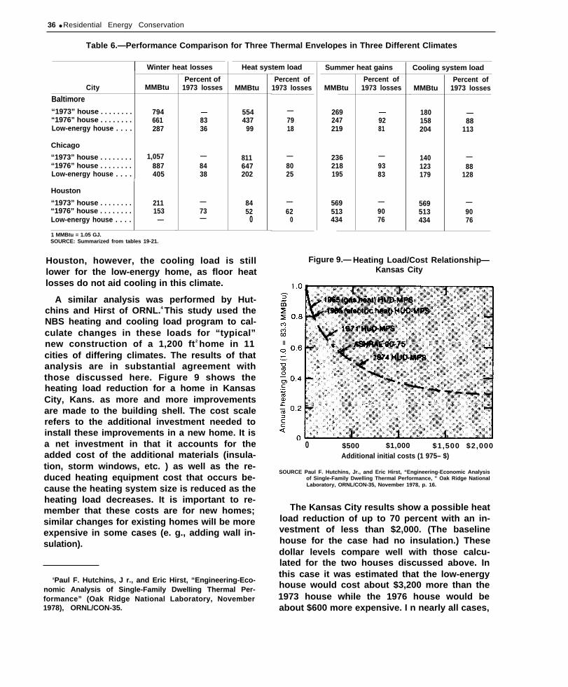


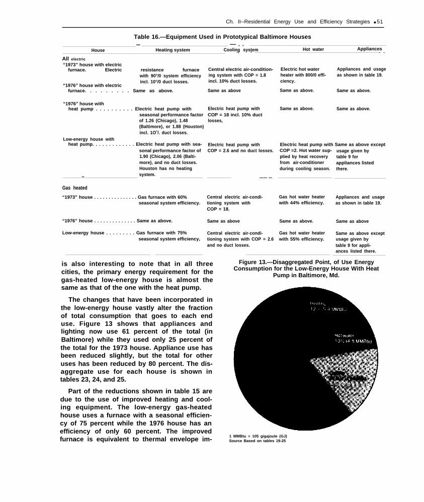


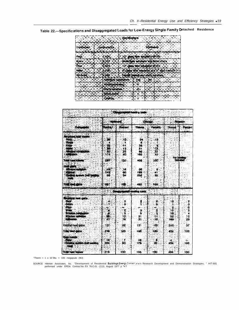


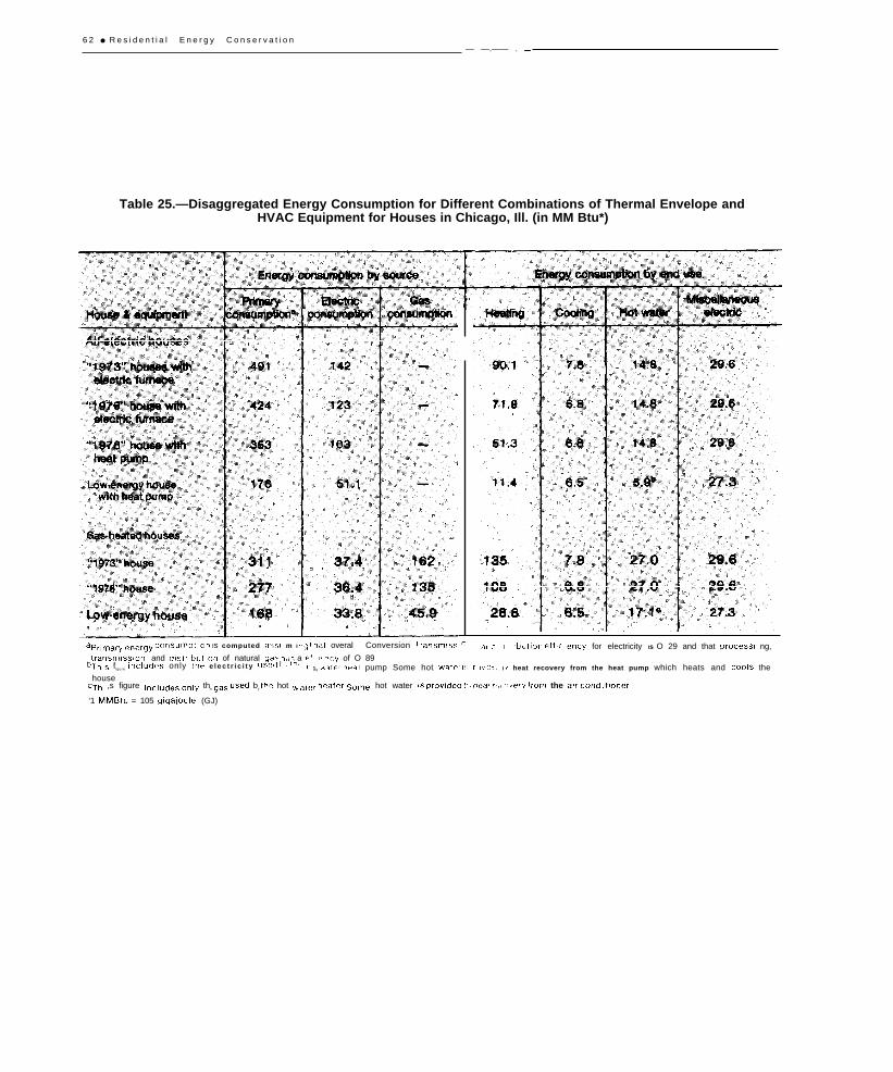


![CHAPTER 4 [RE] RESIDENTIAL ENERGY EFFICIENCY](https://static.documents.pub/doc/80x56/61688a33d394e9041f70624e/chapter-4-re-residential-energy-efficiency.jpg)


