Applied Mathematical Sciences, Vol. 6, 2012, no. 33, 1643 – 1654

Residual Algorithm with Preconditioner

for Linear System of Equations

J. Izadian ∗

Department of Mathematics, Faculty of Sciences, Mashhad Branch, Islamic Azad University, Mashhad, Iran.

Jalal_Izadian@yahoo.com

M. Jalili

Department of Mathematics, Neyshabur Branch, Islamic Azad University, Neyshabur, Iran.

Jalili.maryam@yahoo.com

Abstract One of the most powerful tools for solving large and sparse systems of linear equation is iterative methods. Their significant advantages like low memory requirements and good approximation properties make them very popular, and they are widely used in applications throughout science and engineering. Residual Algorithm for solving large-scale nonsymmetric linear system of equation which symmetric part is positive (or negative) definite, is evaluated. It uses in a systematic way the residual vector as a search direction, and a spectral steplength. The global convergence is analyzed. A preliminary numerical experimentation is included for showing that the new algorithm is a robust method for solving nonsymmetric linear system and it is competitive with the well-known GMRES and BICGSTAB in number of computed residual and CPU time. The new method for sparse matrix with 1210 entries has been successfully examined with we use the two preconditioning strategies ILU and SSOR. Keywords: linear systems, nonsymmetric matrices, preconditioned iterative methods

1644 J. Izadian and M. Jalili 1. Introduction

We introduce an iterative method for solving the linear system of equation

Ax b= (1)

When n nA R ×∈ is nonsymmetric and the symmetric part of A , i.e. ,2

t

sA AA +

=

is positive (or negative) definite, nb R∈ and n is large enough. Different iterative methods have been developed for solving (1). To solve a very large linear system of the form given in (1), especially those derived from3D soil–structure interaction problems, direct solution methods such as sparse LU factorization are impractical from the perspective of computational time and memory requirement. Krylov subspace iterative methods on the other hand, may overcome these difficulties and they are commonly used for solving large-scale linear systems. Three of the most popular Krylov subspace iterative methods for solving the system (1) are SYMMLQ, MINRES and symmetric QMR (SQMR) method. The SYMMLQ and MINRES methods, developed by Paige and Saunders in1975 [6], could only be used in conjunction with symmetric positive definite preconditioners. Unlike the optimal SYMMLQ and MINRES methods, the SQMR method proposed by Freund and Nachtigal [2] can be used in conjunction with a symmetric indefinite preconditioner. Because of this flexibility, we choose to use RA throughout this paper. There are also numerical results showing that RA combined with a symmetric indefinite preconditioner is more effective than a positive definite preconditioner . This paper is organized as follows. In Section 2, we give the model algorithm RA. In Section 3, we give Extensions of the method which we combine RA with a preconditioning method in order to speed up convergence. In Section 4, we consider the application of the RA algorithm for solving large-scale nonsymmetric linear system of equations whose symmetric part is positive (or negative) definite.. In last section, we give a short conclusion. 2 . Model Algorithm Let the functions f and g are given as

:( )

n ng R Rg x Ax b

⎧ →⎨

= −⎩ (2)

2

2

:

( ) ( )

nf R R

f x g x

⎧ →⎪⎨

=⎪⎩ (3)

Residual algorithm with preconditioner 1645 where

2. denotes the Euclidian norm. Now assume that { }kη is a given sequence such

that 0kη > for k N∈ (the set of natural numbers) and

0k

kη η

∞

=

= < ∞∑ . (4)

Suppose min max(0,1) , 0 1γ σ σ∈ < < < , 0α° > and nx R° ∈ is a given arbitary initial point. Combining the systematic use of the search direction, the spectral choice of step length, and the Armijo.test , we obtain the following RA(Residual Algorithm)algorithm. 2-1 RA algorithm Given: 0α° > , min max(0,1) , 0 1γ σ σ∈ < < < ,{ }kη such that (4) holds, and

nx R° ∈ be a sufficiently good initial guess.

Set r b Ax° °= − , and 0k = . Step1 : If 0kr = , stop the process. Step2 : Set 1λ = . Step3 : If

22 22( )k k k k k

k

r Ar r rλ ι γλα

− ≤ + −

go to step5. Step4 : Choose min max[ , ]σ σ σ∈ , set λ σλ← and go to step3. Step5 : Set

1

1

,

( ) ,

( )

k

k k kk

k k kk

x x r

r r Ar

λ λλαλα

+

+

=

= +

= −

Step6 : Set

1 ,

1

tk k

k tk k

r A rr r

k k

α + =

= +

go to step1. A global convergence theorem is presented in [4], that guarantee convergence of the solution of problem (1).

1646 J. Izadian and M. Jalili 3 Extensions of the method

Now, we combine RA with a preconditioning method in order to speed up convergence. 3-1 The preconditioned RA algorithm We suppose that M be a preconditioning matrix. In stead of solving (1) one may as well solve

MAx Mb= (5) or

AMy b= with x My= . (6) Therefore by replacing A by MA and r b Ax° °= − by ( )r M b Ax° °= − we have an algorithm to solve (5) iteratively. In this case the computed residuals

kr are not the real residuals, but ( )k kr M b Ax= − .By replacing A by AM and X x=o o by 1X M x−=o o , we have an algorithm that solves iteratively (6). The computed residuals are the real ones, that is, k kr b AMx= − , but now kx is not the approximated value that we are interested in, we would like to have kMx instead. If we do not want to monitor the approximations of the exact solution x , it suffices to compute kMx only after termination. In both variants, the modified RA algorithm may converges faster, due to the preconditioning. 3-2 SSOR preconditioning The SSOR preconditioner can be derived straight forward from matrix coefficient. The SSOR preconditioner strategies is based on decomposition A as

A L D U= + + (7) where L and U , respectively, are the lower and upper triangular part of A and D is the diagonal part of A . The SSOR matrix is defined as :

1( ) ( )M D L D D U−= + + (8)

3-3 ILU preconditioning The Incompelete LU factorization [1,3], ILU , is probably the best known general purpose preconditioner .We define :

{ }( , ) | 0ijS i j a= ≠ (9)

Residual algorithm with preconditioner 1647 such that ( )ij n nA a ×= .The ILU matrix denote M LU= % % . The ILU factorization, yields :

A LU R= +% % (10) where R ,is the residual matrix representation the difference between A and LU% % .

3-3-1 ILU algorithm for nnijaA ×= )(

Step1 : Do 1:1 −= nr

Step2 : rra

d 1=

Step3 : Do nri :1+= Step4 : If Sri ∈),( then Step5 : irdae = Step6 : eair = Step7 : Do nrj ,1+= Step8 : If Sji ∈),( and Sjr ∈),( then Step9 : rjijij eaaa −= Step10 : End Step11 : End Step12 : End Step13 : End Step14 : End 4. Numerical result In this section we consider the application of the RA algorithm for solving large-scale nonsymmetric linear system of equations whose symmetric part is positive (or negative) definite. For RA algorithm we use the following parameters :

4 3 7min max, 10 , 0.1, 0.9, 10 (1-10 )k

kbα γ σ σ η− − −° = = = = =

We choose a new λ at step4 by following procedure ,given the current 0>cλ we set the new 0λ >

min min

max max

C t C

C t C

t

ifif

otherwise

σ λ λ σ λλ σ λ λ σ λ

λ

<⎧⎪= <⎨⎪⎩

1648 J. Izadian and M. Jalili

where 2 ( )

( ) (2 1) ( )C k

tk C C k

f xf x d f x

λλλ λ

=+ + −

.

The iteration terminated if :

, 0 1krb

ε ε≤ < << , 155 10ε −= × .

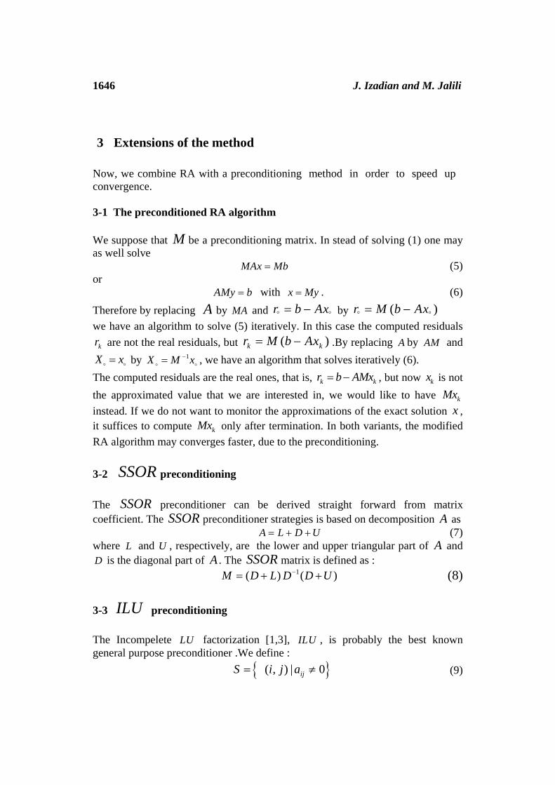
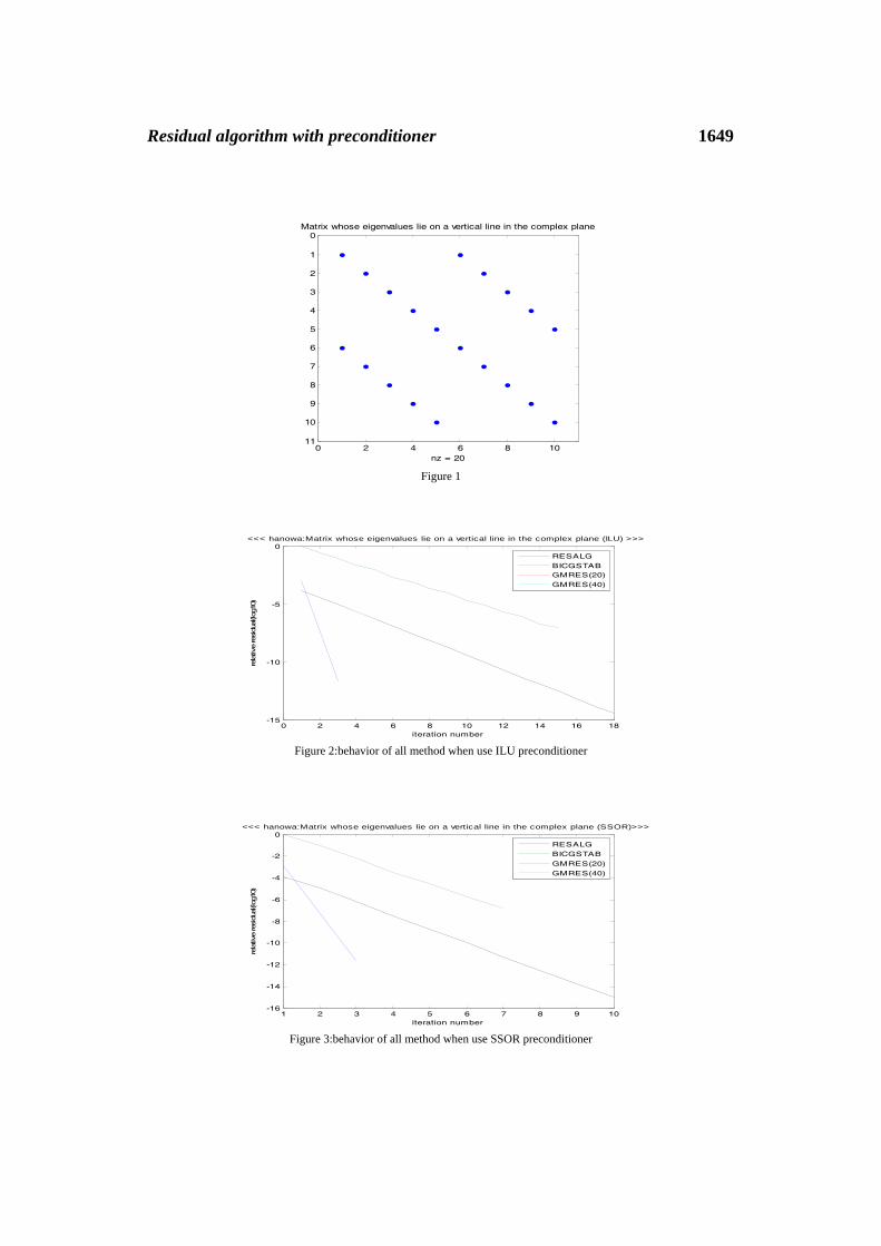
In the numerical result given below, the well-known and well-stablished Krylov subspace methods : BICGSTAB and GMRES [5,7], that restarts every 20 steps( 20m = ), namely (20)GMRES and 40m = ,namely (40)GMRES have been used to solve the given system of linear equations and is compared with RA. We have used a PC-Pentium(R)4 ,CPU 2.4 GHz, 448 MB of RAM and MATLAB R2006a for computations. In all of experiences we have used 0x =o , on the initial guess. In the following numerical experiments, n and " "nnzdenote the order of matrix, and the number of nonzero elements of matrix, respectively. On the other hand iter and CPUtime, refer to number of iteration and elapsed time, respectively. In Table1 we report, the dimension of the problem ( n ); the number of computed residual ( iter ), and elapsed time (sec) until convergence occurred (CPUtime ). Notation : RESALG denote RA in legend figure. 4-1 Example We consider the matrix by MATLAB code (' ', , )A gallery hanowa n n= . We assume that 7000, (1,1,...,1)n b= = and 14000nnz = . The matrix for 10n = is presented in Figure 1. In Figures 2 and 3 we show the behavior of all considered methods when using preconditioning strategies ILU and SSOR .

7000=n

RA BICGSTAB )20(GMRES )40(GMRES

iterCPUtime

iterCPUtime

iterCPUtime

iterCPUtime

ILU 1.48547 3 1.85422 15 2.29685 18 0.34418 18 SSOR 0.98623 3 1.01651 7 1.22560 10 0.68507 10

Table 1

Residual algorithm with preconditioner 1649

Figure 1

Figure 2:behavior of all method when use ILU preconditioner

Figure 3:behavior of all method when use SSOR preconditioner

0 2 4 6 8 10

0

1

2

3

4

5

6

7

8

9

10

11

nz = 20

Matrix whose eigenvalues lie on a vertical line in the complex plane

0 2 4 6 8 10 12 14 16 18-15

-10

-5

0

iteration number

relativ

e re

sidu

al(lo

g10)

<<< hanowa:Matrix whose eigenvalues lie on a vertical line in the complex plane (ILU) >>>

RESALG

BICGSTABGMRES(20)

GMRES(40)

1 2 3 4 5 6 7 8 9 10-16

-14

-12

-10

-8

-6

-4

-2

0

iteration number

relativ

e re

sidu

al(lo

g10)

<<< hanowa:Matrix whose eigenvalues lie on a vertical line in the complex plane (SSOR)>>>

RESALG

BICGSTAB

GMRES(20)

GMRES(40)

1650 J. Izadian and M. Jalili 4-2 Example Consider the matrix by MATLAB code (' ', ,1,10, , 10, 1)A gallery toeppen n n= − − . Let assume that 610n = , (1,1,...,1)b = and 4999994nnz = . The matrix in the case 10n = has been presented in Figure 4, and in Figure 5 we show the behavior of all considered methods when using preconditioning strategies ILU .

610=n RA BICGSTAB )20(GMRES )40(GMRES iterCPUtime

iterCPUtime

iterCPUtime

iterCPUtime

ILU 14.04 2 186.379 2 402.538 3 ∗∗

SSOR 6.0553 2 269.234 1 388.271 2 ∗∗ Table 2

Figure 4

Figure 5:behavior of all method when use ILU preconditioner

0 2 4 6 8 10

0

1

2

3

4

5

6

7

8

9

10

11

nz = 44

Pentadiagonal Toeplitz matrix

1 1.2 1.4 1.6 1.8 2 2.2 2.4 2.6 2.8 3-18

-16

-14

-12

-10

-8

-6

-4

-2

0

iteration number

rela

tive

resi

dual

(log1

0)

<<< toeppen:Pentadiagonal Toeplitz matrix (ILU) >>>

RESALG

BICGSTAB

GMRES(20)

Residual algorithm with preconditioner 1651 4-3 Example We consider the elliptic problem

2 2

sin( )x yxx yyu u e x y−+ = + on the unit square,

whit homogeneous Dirichlet boundary conditions, 0u = , on the border of the region. The discretization grid has 100 internal nodes per axis producing an n n× matrix where 410n = . In Figures 6,7 we show the behavior of all considered methods when using preconditioning strategies ,ILU SSOR ; Figure 8 shows ( , , ( , ))k k k kx y u x y .

410=n RA BICGSTAB )20(GMRES )40(GMRES iterCPUtime

iterCPUtime iterCPUtime iterCPUtime

ILU 0.02297 15 ∗∗ ∗∗ ∗∗

SSOR 5.59485 46 ∗∗ ∗∗ 218.165 501

Table 3

Figure 6:behavior of all method when use ILU preconditioner

Figure 7:behavior of all method when use SSOR preconditioner

0 50 100 150 200 250 300-14

-12

-10

-8

-6

-4

-2

0

2

iteration number

relativ

e re

sidu

al(lo

g10)

<<< The secend order centered differences discretization (ILU) >>>

RESALG

BICGSTAB

GMRES(20)

GMRES(40)

0 100 200 300 400 500 600-16

-14

-12

-10

-8

-6

-4

-2

0

2

iteration number

relativ

e re

sidu

al(lo

g10)

<<< The secend order centered differences discretization (SSOR)>>>

RESALG

BICGSTAB

GMRES(20)

GMRES(40)

1652 J. Izadian and M. Jalili

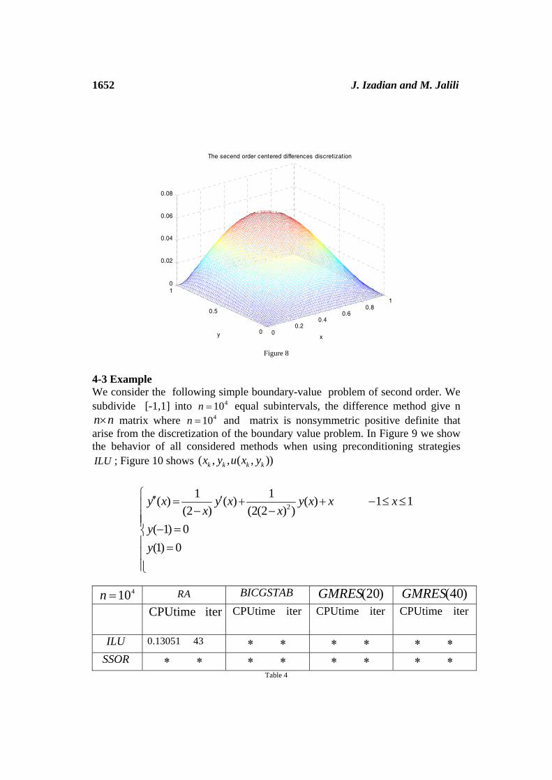
Figure 8

4-3 Example We consider the following simple boundary-value problem of second order. We subdivide [-1,1] into 410n = equal subintervals, the difference method give n n n× matrix where 410n = and matrix is nonsymmetric positive definite that arise from the discretization of the boundary value problem. In Figure 9 we show the behavior of all considered methods when using preconditioning strategies ILU ; Figure 10 shows ( , , ( , ))k k k kx y u x y

2

1 1( ) ( ) ( ) 1 1(2 ) (2(2 ) )

( 1) 0(1) 0

y x y x y x x xx x

yy

⎧ ′′ ′= + + − ≤ ≤⎪ − −⎪⎪ − =⎨⎪ =⎪⎪⎩

410=n RA BICGSTAB )20(GMRES )40(GMRES

iterCPUtime

iterCPUtime iterCPUtime iterCPUtime

ILU 0.13051 43 ∗∗ ∗∗ ∗∗ SSOR ∗∗ ∗∗ ∗∗ ∗∗

Table 4

00.2

0.40.6

0.81

0

0.5

10

0.02

0.04

0.06

0.08

x

The secend order centered differences discretization

y

Residual algorithm with preconditioner 1653

Figure 9:behavior of all method when use ILU preconditioner

Figure 10

5. Conclusions We have interpreted in this paper the RA algorithm, and compare with well-known Krylo subsspase methods, with using two preconditioning strategies ILU and SSOR . We observe that using the residual and spectral step length decrease nonmonotonically norm of the residual and also guarantees convergence. Finally, the numerical results confirm that the RA algorithm presented in this article is worth further application and apply for nonlinear system of equation. References [1] M. Benzi, D.B.Szyld and Arno.V. Duin (1999)." Orderings for Incompeleted Factorization Preconditioning of nonsymmetric problems".SIAM J.SCI.Compute.Vol.20,No.5,PP.1652-1670.

0 100 200 300 400 500 600 700 800-12

-10

-8

-6

-4

-2

0

2

4

iteration number

relativ

e re

sidu

al(lo

g10)

<<< Two point bondary value problem (ILU)>>>

RESALG

GMRES(20)

GMRES(40)

-1 -0.8 -0.6 -0.4 -0.2 0 0.2 0.4 0.6 0.8 1-0.08

-0.06

-0.04

-0.02

0

0.02

0.04

0.06

x

y

<<< Two point bondary value problem >>>

1654 J. Izadian and M. Jalili [2] R.W. Freund, N.M .Nachtigal. A new Krylov-subspace method for symmetric indefinite linear system. In Proceedings [3] S.M. Hosseini and M.Rezghi (2006)." An ILU preconditioner for nonsymmetric positive definite matrices by using conjugate Gram-Schmidt process".Journal of Computational and Applied Mathematics.188-150-164 . [4] W. La Cruzez and M. Raydan (2006)." Residual iterative scheme for large-scale linear systems". Lecturas en Ciencias de la Computación .ISSN 1316-6239. [5] Y. Saad and M. H. Shultz (1986). "GMRES: generalized minimal residual algorithm for solving nonsymmetric linear systems. SIAM J. Sci. Stat". Comput., 7,856–869. [6] CC . Paige, Saunders MA. Solution of sparse indefinite systems of linear equations. SIAM Journal on Numerical Analysis 1975; 12:617– 629. [7] H. A. Van der Vorst (1992). "Bi-CGSTAB: A fast and smoothly convergent variant Bi-CG for the solution of non-symmetric linear systems". SIAM J. Sci. Stat.Comput., 13, 631–644. Received: October, 2011