Resilience to seasonal heat wave episodes in a Mediterranean pine forest Fedor Tatarinov 1 , Eyal Rotenberg 1 , Kadmiel Maseyk 1 ,J er^ ome Ogee 2 , Tamir Klein 1 and Dan Yakir 1 1 Earth & Planetary Sciences, Weizmann Institute of Science, Rehovot 76100, Israel; 2 UMR 1391 ISPA, INRA, Villenave dOrnon 33140, France Author for correspondence: Dan Yakir Tel: +972 89342549 Email: [email protected]Received: 5 September 2015 Accepted: 2 November 2015 New Phytologist (2015) doi: 10.1111/nph.13791 Key words: Aleppo pine (Pinus halepensis), drought, ecosystem activities, ecosystem response, extreme environment, heat wave, resilience. Summary Short-term, intense heat waves (hamsins) are common in the eastern Mediterranean region and provide an opportunity to study the resilience of forests to such events that are predicted to increase in frequency and intensity. The response of a 50-yr-old Aleppo pine (Pinus halepensis) forest to hamsin events lasting 1–7 d was studied using 10 yr of eddy covariance and sap flow measurements. The highest frequency of heat waves was c. four per month, coinciding with the peak pro- ductivity period (March–April). During these events, net ecosystem carbon exchange (NEE) and canopy conductance (g c ) decreased by c. 60%, but evapotranspiration (ET) showed little change. Fast recovery was also observed with fluxes reaching pre-stress values within a day following the event. NEE and g c showed a strong response to vapor pressure deficit that weakened as soil moisture decreased, while sap flow was primarily responding to changes in soil moisture. On an annual scale, heat waves reduced NEE and gross primary productivity by c. 15% and 4%, respectively. Forest resilience to short-term extreme events such as heat waves is probably a key to its survival and must be accounted for to better predict the increasing impact on productivity and survival of such events in future climates. Introduction The current projections for global climate change forecast an increase in the intensity and frequency of extreme climatic events, such as droughts and heat waves (Reichstein et al., 2013; Reyer et al., 2013). In the temperate and boreal regions, the forest trees are typically adapted to a sufficient supply of water and moderate temperatures. Severe heat waves, such as those that occurred in 2003 and 2010, can lead in this case to a considerable decrease in gross primary productivity (GPP) and in net ecosystem CO 2 exchange (NEE), temporarily converting forest ecosystems from sinks to sources of CO 2 (Ciais et al., 2005; Girard et al., 2012) while increasing tree mortality (Allen et al., 2010; Maslov, 2010; Tuzov, 2013) and wildfire frequency (Goldammer, 2010; Shvi- denko & Schepaschenko, 2013). Such events induce a range of ecophysiological responses, but with different effects among tree species. For example, the annual stem basal area increment (BAI) of Fagus sylvatica decreased from 2.8% to 1.3%, whereas the BAIs of Crapinus betulus and Acer campestre were unaffected by heat waves (Leuzinger et al., 2005). Severe drought may lead to the mass mortality of trees from the direct effects of the drought or indirectly from pest attacks (Maslov, 2010; Tuzov, 2013). Less is known about the response of different forests and other ecosystems in warmer biomes in which heat waves occur regu- larly. In the semiarid regions where plants are regularly exposed to water and heat stress for extended parts of the year, increasing the intensity, frequency, or length of droughts can be critical for the survival of forests and other ecosystems (Bonan, 2008). In some studies, resistance to heat waves is observed (Klein et al., 2014). To maintain a functional hydraulic system under dry con- ditions, some tree species may also respond with transient stom- atal closures, but long-term adjustments, such as leaf shedding, changes in the xylem, and cell wall suberization, are also observed (Maseda & Fernandez, 2006; Breda & Badeau, 2008). This study was conducted in a stand of Pinus halepensis (Aleppo pine), which is a common tree species across the Mediterranean region (Neeman & Trabaud, 2000). This pine species survives in a wide range of environmental conditions, from sea level to 2600 m in elevation and from 200 to 1500 mm of annual precipitation. In semiarid climates, the trees are exposed to seasonal heat waves, particularly in spring during the short, peak productivity season, which might affect their overall productivity and survival (Klein et al., 2013). Heat waves in the Mediterranean region are often associated with winds that bring warm, dry air from the desert regions. In the Middle East, such weather events are termed ‘hamsin’ or ‘sharav’. In other parts of the Mediterranean, similar phenomena are also called sirocco (Italy), samum (Morocco), and leveche (Spain). These events are more frequent in the transition seasons, particularly in the spring (Goldreich, 2003). The word ‘hamsin’ Ó 2015 The Authors New Phytologist Ó 2015 New Phytologist Trust New Phytologist (2015) 1 www.newphytologist.com Research
Transcript
Resilience to seasonal heat wave episodes in a Mediterraneanpine forest
Fedor Tatarinov1, Eyal Rotenberg1, Kadmiel Maseyk1, J�erome Og�ee2, Tamir Klein1 and Dan Yakir1
1Earth & Planetary Sciences, Weizmann Institute of Science, Rehovot 76100, Israel; 2UMR 1391 ISPA, INRA, Villenave dOrnon 33140, France
Author for correspondence:Dan YakirTel: +972 89342549
� Short-term, intense heat waves (hamsins) are common in the eastern Mediterranean region
and provide an opportunity to study the resilience of forests to such events that are predicted
to increase in frequency and intensity.� The response of a 50-yr-old Aleppo pine (Pinus halepensis) forest to hamsin events lasting
1–7 d was studied using 10 yr of eddy covariance and sap flow measurements.� The highest frequency of heat waves was c. four per month, coinciding with the peak pro-
ductivity period (March–April). During these events, net ecosystem carbon exchange (NEE)
and canopy conductance (gc) decreased by c. 60%, but evapotranspiration (ET) showed little
change. Fast recovery was also observed with fluxes reaching pre-stress values within a day
following the event. NEE and gc showed a strong response to vapor pressure deficit that
weakened as soil moisture decreased, while sap flow was primarily responding to changes in
soil moisture. On an annual scale, heat waves reduced NEE and gross primary productivity by
c. 15% and 4%, respectively.� Forest resilience to short-term extreme events such as heat waves is probably a key to its
survival and must be accounted for to better predict the increasing impact on productivity and
survival of such events in future climates.
Introduction
The current projections for global climate change forecast anincrease in the intensity and frequency of extreme climatic events,such as droughts and heat waves (Reichstein et al., 2013; Reyeret al., 2013). In the temperate and boreal regions, the forest treesare typically adapted to a sufficient supply of water and moderatetemperatures. Severe heat waves, such as those that occurred in2003 and 2010, can lead in this case to a considerable decrease ingross primary productivity (GPP) and in net ecosystem CO2
exchange (NEE), temporarily converting forest ecosystems fromsinks to sources of CO2 (Ciais et al., 2005; Girard et al., 2012)while increasing tree mortality (Allen et al., 2010; Maslov, 2010;Tuzov, 2013) and wildfire frequency (Goldammer, 2010; Shvi-denko & Schepaschenko, 2013). Such events induce a range ofecophysiological responses, but with different effects among treespecies. For example, the annual stem basal area increment (BAI)of Fagus sylvatica decreased from 2.8% to 1.3%, whereas the BAIsof Crapinus betulus and Acer campestre were unaffected by heatwaves (Leuzinger et al., 2005). Severe drought may lead to themass mortality of trees from the direct effects of the drought orindirectly from pest attacks (Maslov, 2010; Tuzov, 2013).
Less is known about the response of different forests and otherecosystems in warmer biomes in which heat waves occur regu-larly. In the semiarid regions where plants are regularly exposed
to water and heat stress for extended parts of the year, increasingthe intensity, frequency, or length of droughts can be critical forthe survival of forests and other ecosystems (Bonan, 2008). Insome studies, resistance to heat waves is observed (Klein et al.,2014). To maintain a functional hydraulic system under dry con-ditions, some tree species may also respond with transient stom-atal closures, but long-term adjustments, such as leaf shedding,changes in the xylem, and cell wall suberization, are also observed(Maseda & Fernandez, 2006; Breda & Badeau, 2008). Thisstudy was conducted in a stand of Pinus halepensis (Aleppo pine),which is a common tree species across the Mediterranean region(Neeman & Trabaud, 2000). This pine species survives in a widerange of environmental conditions, from sea level to 2600 m inelevation and from 200 to 1500 mm of annual precipitation. Insemiarid climates, the trees are exposed to seasonal heat waves,particularly in spring during the short, peak productivity season,which might affect their overall productivity and survival (Kleinet al., 2013).
Heat waves in the Mediterranean region are often associatedwith winds that bring warm, dry air from the desert regions. Inthe Middle East, such weather events are termed ‘hamsin’ or‘sharav’. In other parts of the Mediterranean, similar phenomenaare also called sirocco (Italy), samum (Morocco), and leveche(Spain). These events are more frequent in the transition seasons,particularly in the spring (Goldreich, 2003). The word ‘hamsin’
� 2015 The Authors
New Phytologist� 2015 New Phytologist Trust
New Phytologist (2015) 1www.newphytologist.com
Research
originates from the Arabic word for ‘fifty’ according to the popu-lar belief that hamsin events occur on c. 50 d yr–1. The typicalhamsin events are characterized by a sharp increase in the temper-ature and the vapor pressure deficit (VPD) to high values of c.35°C and c. 6000 Pa, respectively, over a few days for events thattypically last for 1–7 d. The events are followed by a rapid returnto pre-event values (below 20°C and 1000 Pa) within a day or so,but in some cases, a rain event occurs in the first days following ahamsin event. Thus, there is no commonly accepted definition ofa hamsin event (Goldreich, 2003). It can be defined by thresholdtemperature and humidity values (Gat, 1990) or by deviationfrom long-term mean values based on some threshold (Winstan-ley, 1972; Goldreich, 2003). Under hamsin conditions, airhumidity decreases very rapidly, but such changes are in mostcases too rapid for soil moisture to change significantly, whichoffers an opportunity to distinguish atmospheric from soil mois-ture deficit effects on plant activities.
An important aspect of hamsin events is their high frequency,specifically during the short active season in the semiarid environ-ments (usually in spring; Maseyk et al., 2008a). Would the stresseffects associated with the heat waves be long-lasting, a few ofthese events could eliminate a large fraction of the productive sea-son, enhancing tree mortality. Similarly, productivity and sur-vival can be greatly impacted by the predicted increase in thefrequency and intensity of extreme weather events (Reichsteinet al., 2013; Reyer et al., 2013).
Here we quantify the resilience (i.e. the decline and recovery ofkey functions) to seasonal heat waves of a semiarid pine stand,and test the hypothesis that such resilience is a key factor in itsannual scale productivity, with potential implications for its sur-vival if the frequency of such events were to markedly increase.
Materials and Methods
Study site
The Yatir forest is located at the northern edge of the Negevdesert (30°200N, 35°030E; 650 m above sea level; Rotenberg &Yakir, 2010), covers an area of c. 2800 ha and is dominated byAleppo pine (Pinus halepensis Miller). The primary part of theforest was planted in the mid-1960s. The stand density is c.300 trees ha�1. The soil is a predominantly light brown Rendz-ina, 25–100 cm deep. Pine roots are concentrated mainly inupper 60 cm with the maximum fine root density in the 20–40 cm layer (Gr€unzweig et al., 2007; Klein et al., 2013). The cli-mate is Mediterranean with prolonged summer drought periodsfrom May to October (average daily temperature in July is 25°C)and with a winter period with moderate precipitation (meanannual 290 mm) and temperatures (c. 10°C in January(Gr€unzweig et al., 2007); mean values for 1964–2006).
Measurement system
Begun in 2000, the eddy covariance (EC) and supplementarymeteorological measurements were conducted continuously inthe Yatir forest (Gr€unzweig et al., 2007; Rotenberg & Yakir,
2010). The measurements were performed according to theEuroflux methodology (Aubinet et al., 2000) and were part ofthe European EC sites quality assessment project (G€ockedeet al., 2008). The concentrations of CO2 and water vapor andthe fluxes of NEE (conventionally indicated as negative fluxes,out of the atmosphere) and evapotranspiration (ET, conven-tionally indicated as positive fluxes into the atmosphere) weremeasured continuously using a combination of a sonicanemometer (Gill R-50; Gill Instruments, Lymington, UK)and a closed-path CO2/H2O infrared gas analyzer (IRGA, LI-7000; Li-Cor, Lincoln, NE, USA) with the inlet placed 18.7 mabove ground. The sonic and IRGA variables were used to cal-culate the ecosystem water VPD as the difference between theair saturation humidity derived from the sonic air temperature(corrected for humidity effects by the EC software) and theambient humidity measured directly by the IRGA.
Collected since 2005 (and on-going), soil moisture measure-ments are available for the depths of 5, 15, 30, 50, 70 and 125 cm(Raz Yaseef et al., 2010). The measurements were conducted usingtime-domain reflectometry (TDR) sensors (Trime-PICO 64;IMKO, Ettlingen, Germany) in three pits at depths of 30, 70 and125 cm. Additional soil moisture data in the upper 30 cm werecollected using another TDR sensor (Campbell Scientific, Logan,UT, USA). All soil moisture data were integrated over a 30 mintime step and synchronized with the eddy flux measurements.
Collected since 2004 (and ongoing), tree sap flow was alsomeasured in eight to 24 trees in different years. During 2004–2006, a homemade heat-pulse system (Schiller, 2011; Ungar etal., 2013) was used. Granier-type sensors have been used since2005 (Granier, 1985), and additionally, after 2009, Cermak-type(Cermak et al., 2004) sensors were used (Klein et al., 2012). Sapflow upscaling from tree to stand level is described in Klein et al.(2016) and was performed by averaging sap flux density per unitstem cross-section area among sample trees for each 30 min inter-val and multiplying it by total stand basal area.
Upscaled sap flow (Q, in mm h�1) was used in all further analy-ses to represent the daily tree transpiration Tr. Therefore, the calcu-lations that required the use of Tr, including the canopy daytimeconductance, gc, and the apparent and intrinsic water-use efficiency(W and Wi, respectively) were performed only on a daily basisusing daily GPP andQ values and daytime VPDmean values.
The canopy conductance to CO2 (gc) was calculated as follows(see e.g. Beer et al., 2009):
gc ¼ Q � P=ð1:6 � VPDÞ Eqn 1
where Q and VPD are as noted earlier, P is the daily averageatmospheric pressure, and 1.6 is the ratio of conductance to CO2
and water (reflecting the higher molecular diffusivity of water).The observed gc was corrected for the difference in the VPDbetween that measured above the canopy and that at the level ofthe leaf by the constant correction factor of 1.18, which wasfound suitable for our system as described in Klein et al. (2016).W (in g C kg�1 H2O) was calculated as GPP/Q. Wi was definedas Wi =GPP/gc (Farquhar et al., 1989; Keenan et al., 2013) andwas calculated as:
New Phytologist (2015) � 2015 The Authors
New Phytologist� 2015 New Phytologist Trustwww.newphytologist.com
Research
NewPhytologist2
Wi ¼ W � VPD Eqn 2
Supplementary meteorological variables
Air temperature and humidity at 5 m above the canopy (15 mabove ground) were measured with HMP45C sensor probes andan air pressure sensor (Campbell Scientific). Radiation measure-ments included atmospheric and ecosystem facing solar radiation(CM21; Kipp&Zonen, Delft, the Netherlands). All meteorologi-cal sensors were connected using a differential mode, and the datawere stored as half-hourly means via multiplexers to data loggers(AM16/32, AM25 and two CR10s; Campbell Scientific).
Data gap filling
We used eddy flux and meteorological data measured over 10 yr,which included periods of instrument failures that required datagap filling for estimating daily and annual-scale carbon, water,and energy budgets. We tested the commonly applied algorithmfor NEE gap filling and for carbon flux partitioning into ecosys-tem respiration (Re) and GPP (Reichstein et al., 2005; http://www.bgc-jena.mpg.de/~MDIwork/eddyproc/), but found thatfor the Yatir forest our own site-specific algorithm was more suit-able (Afik, 2009). Briefly, missing NEE values (including theNEE night values when the wind friction velocity, U*, was belowa critical value, Ucrit; Burba, 2013) were filled in with a three-stepalgorithm: (1) missing NEE values were replaced by average NEEvalues for the same time (� 0.5 h) of the days before and after theday with the missing value, using the neighboring 2, 5 or 8 d ifneeded in order to make sure that > 20% of data were availableboth before and after the gap; (2) for the rare occasions where alarger number of days (n) with gaps remained, the values for thesame time (� 1.5 h instead of 0.5 h) from n/2 (if n < 8) or n d (ifn > 8) before and after the gap were used the same way as in (1);(3) when larger gaps remained, the overall mean for the givenhour measured within 30 d of the gap in the active season(November–April), and within 60 d in the nonactive season(summer), was used.
After gap filling, daytime ecosystem respiration (Re-d, inlmol m�2 s�1) was estimated based on measured night-time (i.e.when the global radiation was < 5Wm�2) values (Re-n), averagedfor the first three half-hours of each night. The daytime respira-tion for each half-hour was calculated according to Eqn 3(Maseyk et al., 2008b; Afik, 2009):
Re�d ¼ Re�n � ða1bds Ts þ a2bdwTa þ a3b
dfTa Þ Eqn 3
where bs, bw and bf are coefficients that correspond to soil,wood and foliage, respectively, dTs and dTa are soil and airtemperature deviations from the values at the beginning of thenight, and a1, a2 and a3 are partitioning coefficients fixed at0.5, 0.1 and 0.4, respectively. The bs, bw, and bf coefficientswere calculated as follows: bs = 2.45 for wet soil (soil watercontent in the upper 30 cm above 20% vol); bs = 1.18 for dry
soil (based on the Gr€unzweig et al., 2009 study at the samesite); bf = 3.15 – 0.036Ta; and
bw ¼ 1:34þ 0:46 � exp�� 0:5 � DoY � 162
66:1
� �2�Eqn 4
where DoY is the day of the hydrological year, starting from 1October. Finally, GPP was calculated as GPP =NEE� Re. Nega-tive values of the NEE and GPP indicate that the ecosystem is aCO2 sink.
In total, 82% and 36% of NEE values in the final dataset usedfor further analysis were original values in the daytime and night-time, respectively. During hamsin events, these values reached88% and 43%, respectively. The high proportion of night gaps isthe result of excluding NEE values under low U*. In further anal-ysis, only hamsin events with > 80% of original daytime valueswere used for statistics.
Detection of hamsin events
Hamsin events were detected using a custom-based method wherethe end of the event corresponded to the day when its maximumdaily T and VPD exceeded the corresponding values for the fol-lowing day by > 5°C and > 1100 Pa, respectively. More details onthe method and its testing in comparison to other methods areprovided in the Supporting Information Methods S1.
Statistics
The effect of a specific hamsin event on a variable X was evaluatedby the relative span of X as follows:
rX ¼ ðXb;XaÞ � Xh
X; Eqn 5
where X b, X a and X h are the mean daytime X values for the daybefore the hamsin, the day after the hamsin, and the days of thehamsin, respectively, and X is the overall daytime mean from theday before the hamsin to the day after the hamsin.
The soil moisture conditions were separated into three classes,depending on the soil moisture in the top 30 cm (soil water con-tent (SWC), % vol): dry (SWC < 10%), medium(10 ≤ SWC < 20%) and moist (SWC ≥ 20%).
Results and Discussion
Changes in environmental variables during hamsins
Based on our ‘end-of-hamsin’ detection method applied to thesite’s 10 yr dataset (see Notes S1 and Table S1), hamsin eventswere most frequent during the period from February to June(Fig. 1). Following the precipitation maximum for the rainy sea-son in January (Fig. 1), April was the peak frequency of hamsinevents (three hamsin events per month on average for the studyperiod), which, notably, coincided with the peak in photosyn-thetic activities for this ecosystem (Maseyk et al., 2008a).
� 2015 The Authors
New Phytologist� 2015 New Phytologist TrustNew Phytologist (2015)
Typically, the temperature and VPD increase during the onsetof the event and then fall rapidly at the end of the event, withhigh night-time temperature (Tair) and VPD values (Fig. 2a,b forthe wet and dry periods, respectively), which were typical for anyseason (Table 1). The mean daytime VPD increased comparedwith the day preceding the hamsin by 165% in dry conditions(SWC < 10%) and by over 240% in wetter conditions(SWC > 20%; Table 1), with the highest increase reaching4400 Pa. In addition, the range of VPD variation during a ham-sin event (calculated as the difference between the daytime meanVPD values during an event and the mean daytime VPD values aday before and a day after an event) varied from 1597 Pa (forSWC < 10%) to 1299 Pa (for SWC > 20%; see Table 1). Airtemperature showed similar trends, with a temperature increaseof over 10°C on an event basis in both the wet and dry season(Fig. 2a,b).
The incoming solar radiation (Rg) did not change significantlyduring hamsin events in the dry season, whereas in the wet sea-son, Rg decreased considerably after hamsin events. Simultane-ously, the proportion of diffuse radiation increased considerablyduring, and even more so after, hamsin events (Table 1). Thisresult was probably because the hamsin is usually associated witha cloudless sky but also includes increased dust from the ArabianPeninsula. Following hamsin events, the cloudiness oftenincreases, which is associated with the decreased Rg but also withthe high diffuse radiation. However, the radiation characteristicsdescribed earlier were average responses, and clear skies andreduced diffuse radiation were also observed following hamsinevents.
Ecosystem response to hamsin events
Daytime NEE decreased (i.e. became less negative; with some-what increased, more positive, night-time Re) during the hamsinevents and then fully recovered to pre-event values within the firstday following the end of the event, in both the rainy and dry sea-sons (Figs 2e and f for the wet and dry periods, respectively; seealso Table 1). In relative terms, daytime NEE decreased to 75%,
45% and 0% of its pre-event values with decreasing SWC duringthe drying season (for SWC > 20%, in the range 10–20% and< 10%, respectively; Table 1), but the prehamsin NEE fluxes alsodecreased by c. 90% for the same SWC intervals, from �9.2 to�1.1 lmol m�2 s�1. Following the hamsin events, full recoveryto pre-event values was observed for NEE in the high and inter-mediate SWC conditions. It was also observed in the low SWCconditions for which fluxes were in general very low. Similarresults were obtained for GPP. Full recovery of GPP to pre-eventvalues was also observed immediately following the hamsin, oftenwith some enhancement relatively to prehamsin values in the dri-est conditions.
During hamsin events, both NEE and GPP were linearly cor-related with VPD, the dominant variable during such events,with an overall R2 ranging between 0.2 and 0.8 for individualhamsin events, with the lower values mainly from low flux sum-mer periods (Table 2; see a typical example in Fig. 3b). While thelow fluxes in the dry period make it more difficult to assessecosystem response, the effects of VPD are still apparent, forexample on GPP and gc (Fig. 3b,e), although with different sensi-tivities, as discussed in the following section. Note also that, gen-erally, canopy scale flux measurements show considerable greatervariation than other meteorological measurements (e.g. VPD),somewhat reducing R2 values, especially when these fluxes arelow. Nonetheless, linear relationships improved when a highersolar radiation threshold was used, that is, using midday valuesonly. For example, applying a threshold of Rg > 400Wm�2
resulted in R2 values for NEE or GPP vs VPD that increasedfrom c. 0.4 to 0.7 and 0.6, respectively. This is because daily tran-sition periods with low fluxes and variable light conditions(morning and evening) show the largest deviations from theregression lines in the parameters considered.
The canopy conductance, gc, showed, on average, a strongreduction during hamsin events (down to 17% of the pre-eventin the high SWC conditions; Table 1), and a clear response toVPD in both the wet and dry seasons (Fig. 3e), but also a fastrecovery following the events. Note, however, that gc depends onVPD (Eqn 1), mediated by Q, and therefore reflects a complexresponse to changes in the physical environment and physiologi-cal response. Recovery (and even enhancement) of gc wasobserved at all SWC values after the hamsin events, with valuesbetween 131% and 141% of prehamsin values. This is probablybecause VPD after the hamsin event was usually lower thanbefore the event (Table 1).
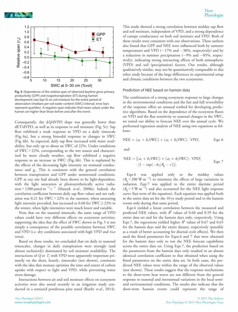
The water fluxes showed a weak and variable response to thehamsin conditions. Indeed, the relative change in ET during ahamsin event (Fig. 4) was, on average, one-third of that for GPP.Daily ET and Q values showed some increase under high SWCconditions and no, or a small, decrease under the drier condi-tions. Similarly, the diurnal courses of both ET and Q did notusually change markedly during hamsins (Fig. 2g,h; Table 1).However, in the spring, ET often decreased considerably follow-ing a hamsin event (Fig. 1g), which was probably associated withthe dramatic decrease in VPD and air temperature at the end ofthe hamsin events, occasionally accompanied by rainfall.Notably, changes in SWC at 5, 15 and 30 cm (Fig. 1c,d) during
1 2 3 4 5 6 7 8 9 10 11 12Month
0
1
2
3
4
5
6
Num
ber o
f ham
sins
per
mon
th
0
20
40
60
80
100
Pre
cipi
tatio
n (m
m m
onth
–1)
Number of hamsinsPrecipitation total
Fig. 1 Median monthly hamsin events (detected by the ‘end-of-hamsin’method), and mean monthly precipitation for 2000–2010 (whiskersrepresent the 25–75% range).
New Phytologist (2015) � 2015 The Authors
New Phytologist� 2015 New Phytologist Trustwww.newphytologist.com
Research
NewPhytologist4
hamsin periods were negligible. Changes in the SWC weredetected only in the top 5 cm layer, which reflected day to nightchanges, and the overall reduction in the volumetric SWC in thislayer through 4 d of a hamsin was only c. 2% in the wet season.
The weak response of the water fluxes to hamsin events proba-bly reflected a tight balance between the effects of the increasing
VPD and decreasing stomatal (and canopy) conductance. Indeed,the large increases in VPD during hamsin events were compen-sated by a marked decrease in gc values (related to a decrease inthe atmosphere to leaf CO2 flux and in the GPP). Accordingly,the dependence of ET and Q on the VPD was associated withlow R2 values, < 0.1 for 84% of events (Fig. 3c; Table 2). The
0
1000
2000
3000
4000
5000
6000
VP
D (P
a)
5
10
15
20
25
30
Air
tem
pera
ture
( OC
)
VPD Tair
(a)
0
1000
2000
3000
4000
5000
6000
VP
D (P
a)
16
20
24
28
32
36
40
Air
tem
pera
ture
( OC
)
(b)
6
8
10
12
14
16
18
20
SW
C (%
vol)
5 cm 15 cm 30 cm
(c)
6
8
10
12
14
16
18
20
SW
C (%
vol)
(d)
–16
–12
–8
–4
0
4
NE
E (
μmol
m–2
s )–1
(e)
–6
–4
–2
0
2
4(f)
9-Apr-10 10-Apr-10 11-Apr-10 12-Apr-10 13-Apr-10
0.0
0.1
0.2
Wat
er fl
ux (m
m h
)
–1
ET Q
(g)
27-Sep-06 29-Sep-06 1-Oct-06
0.0
0.1
0.2
(h)
Wat
er fl
ux (m
m h
)
–1N
EE
( μm
ol m
–2s
)–1
Fig. 2 Typical behavior of climatic and ecosystem variables during 2 d of a hamsin event in the spring (a, c, e, g) and during a 3 d event in the summer (b, d,f, h). Note the different scales in (e) and (f). SWC, soil water content;Q, rate of sap flow; VPD, vapor pressure deficit; NEE, net ecosystem carbonexchange; ET, evapotranspiration.
� 2015 The Authors
New Phytologist� 2015 New Phytologist TrustNew Phytologist (2015)
www.newphytologist.com
NewPhytologist Research 5
only exceptions were spring hamsin events, where R2 for the ET-VPD regressions reached 0.35–0.40. Such cases may occurmostly under high SWC, when soil evaporation, directly depend-ing on VPD, represents a considerable proportion of ET.
The tradeoff between the increasing VPD and leaf conduc-tance was also reflected in the W and Wi values. W decreased, onaverage, during the hamsin events under all SWC conditions,which could be expected because of the decrease in carbon fluxeswith little change in water fluxes (Table 1). The full recovery ofW to pre-event values was observed on the first day following thehamsin in the intermediate and low SWC conditions, but not inthe high SWC conditions. Note, however, that the data werehighly variable, and the changes were significant only in the inter-mediate SWC conditions (Table 1).
Changes in Wi could also be expected, as the relative change ingc was generally greater than for GPP (see Table 1), which couldlead to an increase in Wi. Indeed, Wi values showed a strongincrease during hamsin in the intermediate SWC range, a lowerincrease at high SWC, but little change in the driest conditions(Table 1). Such variations in Wi values reflect a differentialresponse to heat waves between canopy conductance and carbonfluxes, associated with the sensitivity of the carbon fluxes to fac-tors other than gc (e.g. light, temperature, metabolic signals).Generally, on daily to annual timescales, GPP tended to remainproportional to transpiration, which resulted in a relatively con-stant W and Wi on these timescales (Law et al., 2000, 2002).However, other studies, particularly those that examinedMediterranean ecosystems, also reported a decrease in W underlow SWC (Reichstein et al., 2002) or high VPD (Moriana et al.,2002).
Differential response to air and soil moisture
The intense but short-term changes during hamsin events (Fig. 1)involved large changes in atmospheric parameters, such as VPD,
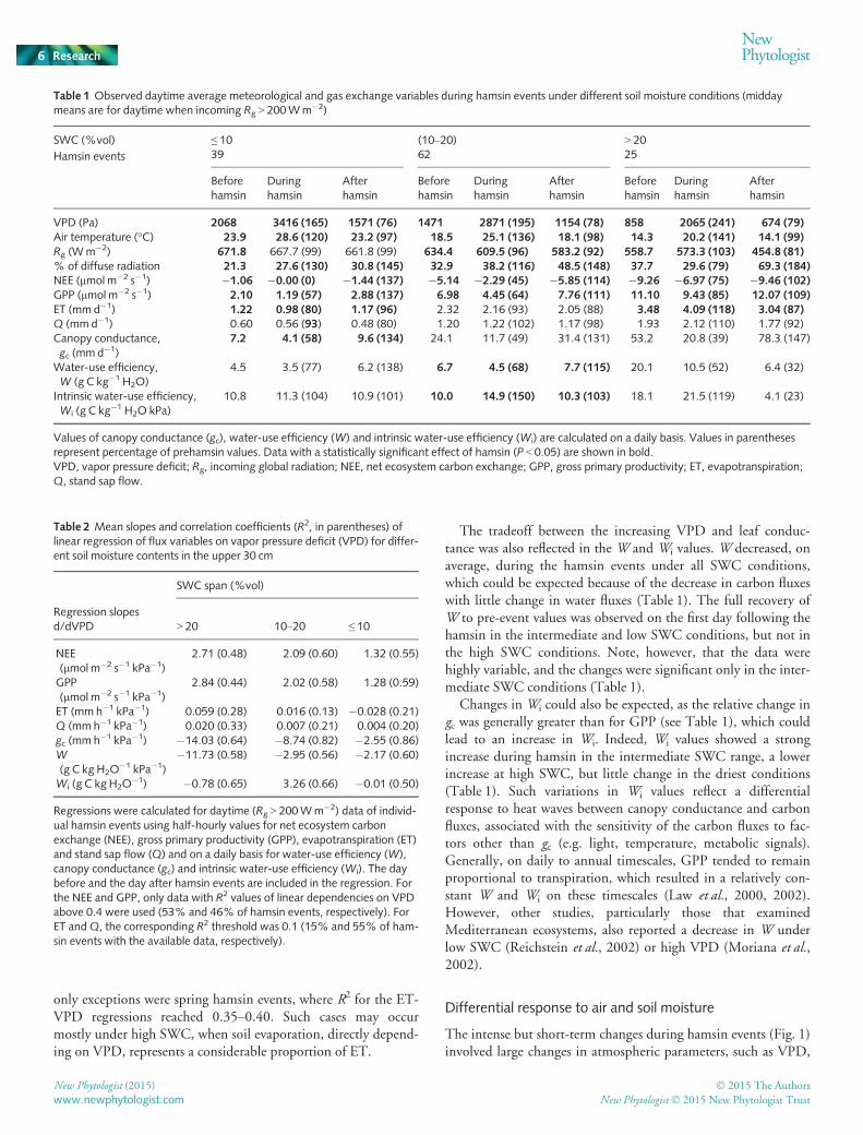
Table 1 Observed daytime average meteorological and gas exchange variables during hamsin events under different soil moisture conditions (middaymeans are for daytime when incoming Rg > 200Wm�2)
Values of canopy conductance (gc), water-use efficiency (W) and intrinsic water-use efficiency (Wi) are calculated on a daily basis. Values in parenthesesrepresent percentage of prehamsin values. Data with a statistically significant effect of hamsin (P < 0.05) are shown in bold.VPD, vapor pressure deficit; Rg, incoming global radiation; NEE, net ecosystem carbon exchange; GPP, gross primary productivity; ET, evapotranspiration;Q, stand sap flow.
Table 2 Mean slopes and correlation coefficients (R2, in parentheses) oflinear regression of flux variables on vapor pressure deficit (VPD) for differ-ent soil moisture contents in the upper 30 cm
Wi (g C kg H2O�1) �0.78 (0.65) 3.26 (0.66) �0.01 (0.50)
Regressions were calculated for daytime (Rg > 200Wm�2) data of individ-ual hamsin events using half-hourly values for net ecosystem carbonexchange (NEE), gross primary productivity (GPP), evapotranspiration (ET)and stand sap flow (Q) and on a daily basis for water-use efficiency (W),canopy conductance (gc) and intrinsic water-use efficiency (Wi). The daybefore and the day after hamsin events are included in the regression. Forthe NEE and GPP, only data with R2 values of linear dependencies on VPDabove 0.4 were used (53% and 46% of hamsin events, respectively). ForET andQ, the corresponding R2 threshold was 0.1 (15% and 55% of ham-sin events with the available data, respectively).
New Phytologist (2015) � 2015 The Authors
New Phytologist� 2015 New Phytologist Trustwww.newphytologist.com
Research
NewPhytologist6
but negligible changes in soil moisture content on the relevanttimescale (few days). However, the occurrence of hamsin eventsthroughout the seasonal drying period at different SWC valuesprovided the opportunity to examine the interactions of theatmospheric (VPD) and soil (SWC) factors on limiting ecosys-tem activities on the longer timescale (seasonal).
A decrease in the sensitivity of ecosystem variables to VPD assoil dries up has been reported previously(Oren et al., 1999;Addington et al., 2004; Gu et al., 2006; Maseyk, 2006). Here, weexamine the interactions of VPD and SWC as reflected in thedependence of the slopes of the linear best-fit lines of dX/dVPDon soil moisture, (where X is a specific ecosystem variable; Fig. 5).The observed dNEE/dVPD and dGPP/dVPD showed directdependence on soil moisture (Fig. 5a,b), with decreasing sensitiv-ity (decreasing slope) of dNEE/dVPD and dGPP/dVPD with
decreasing soil moisture (relatively low R2 values reflect the rela-tively small fluxes and their sensitivity to a wide range of factors).This dependence was stronger for SWC at the depths of 5 and15 cm than for SWC at 30 cm (only data for 15 cm are shown).These observations clearly demonstrated that as the soil dries out,soil moisture availability becomes the dominant factor, overVPD, in limiting ecosystem activities, with most functions ulti-mately becoming insensitive to VPD.
The interactions of the water fluxes, ET and Tr, with VPD andSWC were more complex. As noted earlier, under high soil mois-ture conditions, ET reflects the effects of VPD on soil evapora-tion. This can explain the observations reported in Fig. 5(d),showing increased sensitivity of ET to VPD with increasing soilmoisture. By contrast, Tr, represented by measured sap flow, isinfluenced by the interactions of gc and VPD noted earlier.
0
1000
2000
3000
4000
5000
6000
0 1 2 3 4 5
VPD
(Pa)
Time (d)
26-30.09.20069-13.04.2010
(a) –14
–12
–10
–8
–6
–4
–2
00 1000 2000 3000 4000 5000
GPP
(µm
ol m
–2s
)–1
VPD (Pa)
(b)
0
0.04
0.08
0.12
0.16
0 1000 2000 3000 4000 5000
ET (m
m h
)
–1
VPD (Pa)
(c)
0
0.01
0.02
0.03
0.04
0.05
0.06
0.07
0.08
0.09
0 1000 2000 3000 4000 5000
Q (m
m h
)
–1
VPD (Pa)
(d)
0
10
20
30
40
50
60
70
0 1000 2000 3000 4000 5000
g c (m
m d
)
–1
VPD (Pa) VPD (Pa)
(e)
0
1
2
3
4
5
6
7
8
9
0 1000 2000 3000 4000 5000
W (g
C k
g–1
H2 O
)
(f)
R2 = 0.47
R2 = 0.00
R2 = 0.37
R2 = 0.86
R2 = 0.10
R2 = 0.78
R2 = 0.30 R2 = 0.66
R2 = 0.01
R2 = 0.16
Fig. 3 Changes in vapor pressure deficit(VPD) during hamsin events (a; x-axisincludes the day before and after the event),and examples of the dependence on VPD ofobserved daytime (Rg > 200Wm�2) valuesof ecosystem variables during spring (bluelines and symbols) and summer (red lines andsymbols) hamsin events (b–f). GPP, grossprimary productivity; ET, evapotranspiration;Q, sap flow; gc, canopy conductance;W,water-use efficiency. Darker points on (b–f)correspond to later days. R2 values on thegraphs are calculated on a half-hourly base.
� 2015 The Authors
New Phytologist� 2015 New Phytologist TrustNew Phytologist (2015)
www.newphytologist.com
NewPhytologist Research 7
Consequently, the dQ/dVPD slope was generally lower thandET/dVPD, as well as its response to soil moisture (Fig. 5c). Sapflow exhibited a weak response to VPD on a daily timescale(Fig. 6a), but a strong bimodal response to changes in SWC(Fig. 6b). As expected, daily sap flow increased with water avail-ability, but only up to about an SWC of 22%. Under conditionsof SWC > 22%, corresponding to the wet season and character-ized by more cloudy weather, sap flow exhibited a negativeresponse to an increase in SWC (Fig. 6b). This is explained bythe effects of the decreasing light intensity on stomatal conduc-tance and gc. This is consistent with the general correlationbetween transpiration and GPP under nonstressed conditions.GPP at our site had already been shown to be light-dependent,with the light saturation at photosynthetically active radia-tion > 1200 lmol m�2 s�1 (Maseyk et al., 2008a). Indeed, thecorrelation coefficient between daily sap flow values and net radi-ation was 0.21 for SWC < 22% in the summer, when saturatinglight intensity prevailed, but increased to 0.60 for SWC ≥ 22% inthe winter, when light intensities were much lower and variable.
Note that on the seasonal timescale, the same range of VPDvalues could have very different effects on ecosystem activities,supporting the idea that the effect of SWC shown in Fig. 5 is notsimply a consequence of the possible correlation between SWCand VPD (i.e. dry conditions associated with high VPD and viceversa).
Based on these results, we concluded that on daily to seasonaltimescales, changes in daily transpiration were strongly (andalmost exclusively) dominated by soil moisture availability. Theinteractions of Q or Tr with VPD were apparently important pri-marily on the short, hourly, timescales (not shown), consistentwith the idea that stomata optimize the time and extent of carbonuptake with respect to light and VPD, while preventing waterstress damage.
Interactions between air and soil moisture effects on ecosystemactivities were also noted recently in an irrigation study con-ducted in a semiarid ponderosa pine stand (Ruehr et al., 2014).
This study showed a strong correlation between midday sap flowand soil moisture, independent of VPD, and a strong dependenceof canopy conductance on both soil moisture and VPD. Both ofthese results were consistent with our observations. These authorsalso found that GPP and NEE were influenced both by summertemperatures and VPD (�17% and �38%, respectively) and bya reduction in summer precipitation (�9% and �85%, respec-tively), indicating strong interacting effects of both atmospheric(VPD) and soil (precipitation) factors. Our results, althoughqualitatively similar, may not be quantitatively comparable to thisother study because of the large differences in experimental setupand climatic conditions between the two ecosystems.
Prediction of NEE based on hamsin data
The combination of a strong ecosystem response to large changesin the environmental conditions and the fast and full reversibilityof the response offers an unusual testbed for developing predic-tive algorithms. Based on the dependence of the ecosystem fluxeson VPD and the flux sensitivity to seasonal changes in the SWC,we tested our ability to forecast NEE over the annual cycle. Weperformed regression analysis of NEE using two equations as fol-lows:
Eqn 6 was applied only to the midday values(Rg > 200Wm�2) to minimize the effects of large variations inradiation. Eqn 7 was applied to the entire daytime period(Rg > 5Wm�2) and also accounted for the NEE light responsecurve (last term of the equation). Each equation was applied bothto the entire data set for the 10 yr study period and to the hamsinevents only during that same period.
Eqn 6 yielded a linear correlation between the measured andpredicted NEE values, with R2 values of 0.60 and 0.59 for theentire data set and for the hamsin days only, respectively. UsingEqn 7, the regressions yielded higher R2 values of 0.67 and 0.65for the hamsin days and the entire dataset, respectively (possiblyas a result of better accounting for diurnal cycle effects). We thenused the fitted parameters for Eqns 6 and 7 that were obtainedfor the hamsin days only to test the NEE forecast capabilitiesacross the entire data set. Using Eqn 7, the prediction based onthe parameters from the hamsin days only resulted in an almostidentical correlation coefficient to that obtained when using thefitted parameters on the entire data set. In both cases, the pre-dicted NEE values were within the range of the observed values(not shown). These results suggest that the response mechanismsto the short-term heat waves are not different from the generalresponse to seasonal and interannual variations in the local semi-arid environmental conditions. The results also indicate that theshort-term hamsin events could represent the range of
5 10 15 20 25 30SWC at 0–30 cm (%vol)
–0.8–0.6–0.4–0.20.00.20.40.60.81.01.2
Rel
ativ
e sp
an (r
x)
GPP ET
Fig. 4 Dependence of the relative span of observed daytime gross primaryproductivity (GPP) and evapotranspiration (ET) during hamsindevelopment (see Eqn 5) on soil moisture for the entire period ofobservation (medians per soil water content (SWC) interval; error barsrepresent quartiles). A negative span indicates that mean values under thehamsin are higher than those before and after the event.
New Phytologist (2015) � 2015 The Authors
New Phytologist� 2015 New Phytologist Trustwww.newphytologist.com
Research
NewPhytologist8
environmental variations that would otherwise require a muchlonger observation period.
Effects of hamsins on annual NEE
The strong reduction in carbon uptake (NEE or GPP; Fig. 1)during hamsin events, combined with the high frequency of suchevents at the peak activity period (Fig. 2) implies that the fre-quency and intensity of the events could significantly influencethe annual productivity of the forest. By contrast, the high degreeof resilience greatly reduces the extent of the hamsin effects andallows maximum productivity (NEE), even when intervalsbetween events are short.
To assess the combined effects of heat waves and resilience onthe annual carbon budget of the forest, the relative differencebetween the actual mean annual NEE was compared with themean NEE assuming that no hamsin events had occurred,according to:
a ¼ NEE�NEE�ð ÞNEE� Eqn 8
NEE* and NEE are the annual net CO2 exchange flux excludingor including hamsin days, respectively, where:NEE� ¼ F no hamsin � ðNhamsin þNno hamsinÞ; andNEE ¼ F no hamsin�
Nno hamsin þ F hamsin �Nhamsin and where N and F are the numberof days yr–1 and the mean daily net CO2 flux (during hamsin ornot, as indicated), respectively. The effects on the GPP were esti-mated in a similar way.
This analysis indicated that annual average NEE and GPPduring the study period were reduced by the hamsin eventsby 15.4% and 4.2%, respectively (in total, hamsin days con-stituted 10.4% of the study period). Note, however, that forthe average NEE and GPP fluxes of �44.4 and�159.1 mmol m�2 d�1, respectively, the percentage differencestranslate to a similar quantity of 6.8 and 6.7 mmol m�2 d�1.Remembering that NEE =GPP + Re, the results indicate that,on average, hamsin events influenced predominantly GPP, theleaf photosynthetic CO2 flux. The proportionally large effectson NEE reflect the fact that it is a small residual flux of twolarge opposing fluxes of GPP and Re and, accordingly, annualRe did not change significantly as a result of hamsin effects(annual average Re was 115 mmol m�2 d�1, both includingand excluding hamsin events). Finally, we note that theannual-scale analysis can also be used to assess the importanceof the resilience component. For example, extending hamsinevents by 3 d on average during the wet season (February–May) would decrease annual NEE by c. 28% compared withthe no-hamsin scenario (with a smaller effect during summerwhen fluxes are small).
0
0.5
1
1.5
2
2.5
3
3.5
4
4.5
5(a) (b)
(c) (d)
8 10 12 14 16 18 20 22
dNEE
/dV
PD (µ
mol
m–2
s–1
kPa
–1)
dGPP
/dV
PD (µ
mol
m–2
s–1
kPa
–1)
SWC at 15 cm (%vol) SWC at 15 cm (%vol)
y = 0.22x – 0.85, R² = 0.55
0
0.5
1
1.5
2
2.5
3
3.5
4
4.5
5
8 10 12 14 16 18 20 22
y = 0.20x – 0.70, R² = 0.32
–0.05
–0.03
–0.01
0.01
0.03
0.05
0.07
0.09
0.11
5 10 15 20 25 30 35 40 45
y = 0.002x – 0.015, R² = 0.67
dQ/d
VPD
(mm
h–1
kPa
–1)
SWC above 30 cm (%vol) SWC above 30 cm (%vol)–0.05
–0.03
–0.01
0.01
0.03
0.05
0.07
0.09
0.11
5 10 15 20 25 30 35 40 45dET/
dVPD
(mm
h–1
kPa
–1)
y = 0.003x – 0.037, R² = 0.75
Fig. 5 Dependence of net ecosystem carbon exchange (NEE; a), gross primary productivity (GPP; b), sap flow (Q; c), and evapotranspiration (ET; d)sensitivity to vapor pressure deficit (VPD) (slope of linear correlation) on the soil water content (SWC) at different depths (depths with the best dependencewere selected) along the seasonal cycle. All slopes were calculated for daytime values (Rg > 200Wm�2). For the NEE and GPP, only data with R2 values forcorresponding dependences on VPD above 0.4 were used (53% and 46% of hamsin events, respectively). For ET andQ, the R2 threshold was 0.1 (55% ofhamsin events with the available data).
� 2015 The Authors
New Phytologist� 2015 New Phytologist TrustNew Phytologist (2015)
www.newphytologist.com
NewPhytologist Research 9
It is generally accepted that major episodic heat waves in tem-perate regions lead to large decreases in ecosystem productivity(Baldocchi, 1997; Ciais et al., 2005; Reichstein et al., 2013). Fur-thermore, after droughts, forests often require long recovery peri-ods (from months to several years). In particular, heat waves anddroughts can result in irreversible photoinhibition, mortality offoliage, branches or entire trees, and enhanced pest attacks,among other types of damage to the forest (Brodribb, 1996;
Reichstein et al., 2013; Saatchi et al., 2013), including irreversiblechanges in forest composition (Cavin et al., 2013). Our resultshave shown that in the case of the pine ecosystem adapted tosemiarid conditions (Weinstein, 1989; Rotenberg & Yakir, 2010;Schiller, 2011), a high degree of resilience was achieved, withrapid full recovery and no irreversible damage associated with theshort but intense heat wave events, with the highest frequencyduring the short peak activity period. We suggest that this
Mean daily VPD (Pa)
Sap
flow
(l d
)
–1S
ap fl
ow (l
d
)–1
0 1000 2000 3000 4000 5000 60000.0
0.2
0.4
0.6
0.8
1.0
1.2
1.4
1.6
1.8
SWC ≤ 22: y = 0.3546 + 1.9991E-5*x; r 2 = 0.01SWC > 22: y = 0.4819 + 0.0002*x; r 2 = 0.29
Mean daily SWC (%vol)5 10 15 20 25 30 35 40 45
0.0
0.2
0.4
0.6
0.8
1.0
1.2
1.4
1.6
1.8
SWC ≤ 22: y = –0.3518 + 0.0664*x; r 2 = 0.64SWC > 22: y = 1.5126 – 0.0275*x; r 2 = 0.20
(b)
(a)
1000 2000 3000 4000
VPD (Pa)
0.0
0.2
0.4
0.6
5 10 15 20 25 30 35
Mean daily SWC at 0–30 cm (%vol)
0.0
0.5
1.0
1.5
Sap
flow
(mm
d
)–1
Sap
flow
(mm
d
)–1
Fig. 6 Dependence of measured sap flowdaily totals on mean daily vapor pressuredeficit (VPD) (a) and soil water content(SWC) at 0–30 cm, separately forSWC < 22% and SWC ≥ 22%, in the upperlayer (b), for the study period 2001–2010.The inserts represent medians and quartilesof sap flow daily totals by VPD (a) and SWC(b) classes.
New Phytologist (2015) � 2015 The Authors
New Phytologist� 2015 New Phytologist Trustwww.newphytologist.com
Research
NewPhytologist10
resilience is probably a key to the survival and productivity of theforest in a harsh environment, which may become the prevalentenvironment in many currently wetter regions. The results of thisstudy also demonstrate the utility of short-term heat waves instudying the response of forest ecosystems to stress and in separat-ing the effects of atmospheric (VPD and temperature) factorsfrom those of the soil (SWC).
Acknowledgements
Different parts of this long-term work were supported by KKL-JNF, The Cathy Wills and Robert Lewis Program in Environ-mental Science, the Israel Science Foundation (ISF), the IsraeliWater Authority, and the High Council for Scientific and Tech-nological Cooperation between France and Israel (contract ref.09 F2/ENERGY). The authors thank Drs Shabtai Cohen andGabriel Schiller from the ARO Volcani Center, Israel, for provid-ing early period sap flow data, and Tal Kaneti for assistance insap flow sensor manufacturing.
Author contributions
D.Y., E.R., T.K. and K.M. planned and designed the research;E.R. was responsible for eddy covariance data, T.K. for sap-flowdata, K.M. for physiological data, and J.O. supplied supportingmodel simulation. F.T. performed data analysis and wrote thefirst draft of the manuscript, which was revised and expanded byall co-authors.
vapor pressure deficit and its relationship to hydraulic conductance in Pinuspalustris. Tree Physiology 24: 561–569.
Afik T. 2009. Quantitative estimation of CO2 fluxes in a semi-arid forest and theirdependence on climatic factors. Thesis submitted to R.H. Smith Faculty of
Agriculture, Food and Environment of Hebrew University, Rehovot, Israel (in
Hebrew).
Allen CD, Macalady AK, Chenchouni H, Bachelet D, McDowell N,
Vennetier M, Kitzberger T, Rigling A, Breshears DD, Hogg EH et al.2010. A global overview of drought and heat-induced tree mortality reveals
emerging climate change risks for forests. Forest Ecology and Management259: 660–684.
Aubinet M, Grelle A, Ibrom A, Rannik U, Moncrieff J, Foken T,
Kowalski AS, Martin PH, Berbigier P, Bernhofer Ch et al. 2000.Estimates of the annual net carbon and water exchange of European
forests: the EUROFLUX methodology. Advances in Ecological Research 30:
113–175.Baldocchi D. 1997.Measuring and modeling carbon dioxide and water vapour
exchange over a temperate broad-leaved forest during the 1995 summer
drought. Plant, Cell & Environment 20: 1108–1122.Beer C, Ciais P, Reichstein M, Baldocchi D, Law BE, Papale D, Soussana J-F,
Ammann C, Buchmann N, Frank D et al. 2009. Temporal and among-site
variability of inherent water use efficiency at the ecosystem level. GlobalBiogeochemical Cycles 23: GB2018.
Bonan G. 2008. Forests and climate change: forcings, feedbacks, and the climate
benefits of forests. Science 320: 1444–1449.Breda N, Badeau V. 2008. Forest tree responses to extreme drought and some
biotic events: towards a selection according to hazard tolerance? Comptes RendusGeoscience 340: 651–662.
Brodribb T. 1996. Dynamics of changing intercellular CO2 concentration (ci)
during drought and determination of minimum functional ci. Plant Physiology111: 179–185.
Burba G. 2013. Eddy covariance method for scientific, industrial, agricultural, andregulatory applications. Lincoln, NE, USA: LI-COR Biosciences.
dioxide and water vapor exchange of terrestrial vegetation. Agricultural andForest Meteorology 113: 97–120.
Law BE, Williams M, Anthoni PM, Baldocchi DD, Unswort MH. 2000.
Measuring and modelling seasonal variation of carbon dioxide and water
vapour exchange of a Pinus ponderosa forest subject to soil water deficit. GlobalChange Biology 6: 613–630.
Leuzinger S, Zotz G, Asshoff R, K€orner C. 2005. Responses of deciduous forest
trees to severe drought in Central Europe. Tree Physiology 25: 641–650.Maseda PH, Fernandez RJ. 2006. Stay wet or else: three ways in which plants can
adjust hydraulically to their environment. Journal of Experimental Botany 57:3963–3977.
Maseyk KS. 2006. Ecophysiological and phonological aspects of Pinus halepensisin an arid-Mediterranean environment. PhD thesis, Weizmann Institute of
Science, Rehovot, Israel.
Maseyk KS, Gr€unzweig JM, Rotenberg E, Yakir D. 2008b. Respiration
acclimation contributes to high carbon-use efficiency in a seasonally dry pine
forest. Global Change Biology 14: 1553–1567.Maseyk KS, Lin T, Rotenberg E, Gr€unzweig JM, Schwartz A, Yakir D. 2008a.
Physiology–phenology interactions in a productive semi-arid pine forest. NewPhytologist 178: 603–616.
Maslov AD. 2010. Koroyed-tipograf I usychanie yelovych lesov. “Bark printing beetleand drying up of spruce forest”. Moscow, Russia: VNIILM (in Russian).
Moriana A, Villalobos FJ, Fereres E. 2002. Stomatal and photosynthetic
responses of olive (Olea europaea L.) leaves to water deficits. Plant, Cell &Environment 25: 395–405.
Neeman G, Trabaud L, eds. 2000. Ecology, biogeography and management ofPinus halepensis and P. brutia forest ecosystems in the Mediterranean Basin.Leiden, the Netherlands: Backhuys Pub.
Oren R, Sperry JS, Katul GG, Pataki DE, Ewers BE, Phillips N, Sch€afer KVR.1999. Survey and synthesis of intra- and interspecific variation in stomatal
Raz Yaseef N, Yakir D, Rotenberg E, Schiller G, Cohen S. 2010. Ecohydrology
of a semi-arid forest: partitioning among water balance components and its
implications for predicted precipitation changes. Ecohydrology 3: 143–154.Reichstein M, Bahn M, Ciais P, Frank D, Mahecha MD, Seneviratne SI,
Zscheischler J, Beer C, Buchmann N, Frank DC et al. 2013. Climate extremes
and the carbon cycle. Nature 500: 287–295.Reichstein M, Falge E, Baldocci D, Papale D, Aubinet M, Berbigier P,
Bernhofer Ch, Buchmann N, Gilmanov T, Granier A et al. 2005.On the
separation of net ecosystem exchange into assimilation and ecosystem
respiration: review and improved algorithm. Global Change Biology 11–3:1424–1439.
Reichstein M, Tenhunen JD, Roupsard O, Ourcival J-M, Rambal S, Miglietta
F, Peressotti A, Pecchiari M, Tirone G, Valentini R. 2002. Severe drought
effects on ecosystem CO2 and H2O fluxes at three Mediterranean evergreen
sites: revision of current hypotheses? Global Change Biology 8: 999–1017.Reyer CPO, Leuzinger S, Rammig A, Wolf A, Bartholomeus RP, Bonfante A,
de Lorenzi F, Dury M, Gloning P, Abou Jaoud�e R et al. 2013. A plant’s
perspective of extremes: terrestrial plant responses to changing climatic
variability. Global Change Biology 19–1: 1365–2486.Rotenberg E, Yakir D. 2010. Contribution of semi-arid forests to the climate
system. Science 327: 451–454.Ruehr NK, Law BE, Quandt D, Williams M. 2014. Effects of heat and drought
on carbon and water dynamics in a regenerating semi-arid pine forest: a
combined experimental and modeling approach. Biogeosciences 11: 4139–4156.Saatchi S, Asefi-Najafabady S, Malhi Y, Arag~ao LEOC, Anderson LO, Myneni
RB, Nemani R. 2013. Persistent effects of a severe drought on Amazonian forest
canopy. Proceedings of the National Academy of Sciences, USA 110: 565–570.Schiller G. 2011. The case of Yatir Forest. In: Bredemeier M, Cohen S, Godbold
DL, Lode E, Pichler V, Schleppi P, eds. Forest management and the water cycle:an ecosystem-based approach. Ecological Studies 212: 163–186.
Shvidenko AZ, Schepaschenko DG. 2013. Climate change and wildfires in
Russia. Contemporary Problems of Ecology 6: 683–692.Tuzov VK. 2013. “Outbreak of bark beetle in European part of Russia and measuresfor eliminate its consequences”. Problems of dying of spruce stands. Proceedings ofInternational Scientific and Practical Seminar, 26–27 September 2013,
Mogilyov, Belarus. Minsk, Belarus: Colorpoint Publishers, 22–24.Ungar ED, Rotenberg E, Raz-Yaseef N, Cohen S, Yakir D, Schiller G. 2013.
Transpiration and annual water balance of Aleppo pine in a semiarid region:
implications for forest management. Forest Ecology and Management 298: 39–51.
Weinstein A. 1989. Geographic variation and phenology of Pinus halepensis, P.brutia and P. eldarica in Israel. Forest Ecology and Management 27: 99–108.
Winstanley D. 1972. Sharav.Weather 27: 146–160.
Supporting Information
Additional supporting information may be found in the onlineversion of this article.
Table S1 Comparison of different hamsin detection algorithmswith manual detection for the years 2001–2007
Methods S1 Detection of hamsin events.
Notes S1 Results of comparison of hamsin detection by differentmethods.
Please note: Wiley Blackwell are not responsible for the contentor functionality of any supporting information supplied by theauthors. Any queries (other than missing material) should bedirected to the New Phytologist Central Office.
New Phytologist (2015) � 2015 The Authors
New Phytologist� 2015 New Phytologist Trustwww.newphytologist.com