SHRP-C-391 Resistance of Concrete to Freezing and Thawing Donald J. Janssen University of Washington Seattle, Washington 98195 Mark B. Snyder University of Minnesota Minneapolis, Minnesota 55455 Strategic Highway Research Program National Research Council Washington, DC 1994
Transcript
SHRP-C-391
Resistance of Concrete
to Freezing and Thawing
Donald J. JanssenUniversity of Washington
Seattle, Washington 98195
Mark B. SnyderUniversity of Minnesota
Minneapolis, Minnesota 55455
Strategic Highway Research ProgramNational Research Council
Washington, DC 1994
SHRP-C-391Contract C-203ISBN 0-309-05773-6
Product no. 2002, 2004, 2018, 2019, 2020, 2021
Program Manager: Don M. HarriottProject Manager: Inam JawedEditor: Katharyn L. BineProduction Editors: Carina S. Hreib, Carrie Kent
June 1994
key words:aggregateD-crackingdurability factorfreezing and thawingmodal analysisportland cement concretequality factorresonance frequency
Strategic Highway Research ProgramNational Research Council2101 Constitution Avenue N.W.
Washington, DC 20418
(202) 334-3774
The publication of this report does not necessarily indicate approval or endorsement by the National Academy ofSciences, the United States Government, or the American Association of State Highway and TransportationOfficials or its member states of the findings, opinions, conclusions, or recommendations either inferred or
The research described herein was supported by the Strategic Highway Research Program(SHRP). SHRP is a unit of the National Research Council that was authorized by section128 of the Surface Transportation and Uniform Relocation Assistance Act of 1987.
This book represents the efforts of many people and organizations. Appendix D, "DampingMeasurements for Nondestructive Evaluation of Concrete Beams," was a collaborative workby Elizabeth A. Vokes, Washington State Department of Transportation; Steven L. Clarke,Archos, Inc.; Donald J. Janssen, University of Washington; and the Washington StateTransportation Center (TRAC). The National Science Foundation provided some of the TestEquipment used in this particular study. J. D. Chalupnik and D. W. Storti, Department ofChemical Engineering, and W. D. Scott, Department of Material Science and Engineeringassisted in the development of the initial impulse-excitation procedures. Additional supportcame from the National Science Foundation and in-kind support from Michigan StateUniversity and the University of Washington.
iii
Preface
The mechanisms of damage to concrete from repeated cycles of freezing and thawing are notwell understood and continue to be intensively studied. Original research was based on thefact that water expands 9 percent when it freezes. Thus, the term "critical saturation" wascoined to describe the point at which the concrete pores were 91.7 percent saturated and,therefore, assumed to be susceptible to damage due to freezing and thawing. Furtherinvestigation determined that deterioration due to freezing and thawing can affect concretewith lower degrees of saturation.1
Four theories have gained wide acceptance in describing the mechanisms of frost action. 2Although most of these theories were originally used to describe the frost action in cementpaste, they are also applicable to concrete. 3 The first was the hydraulic pressure theoryPowers proposed in 1945. This was followed by the diffusion and growth of capillary icetheory constructed by Powers and Helmuth in 1953, the dual mechanism theory by Larsonand Cady in 1969, and the desorption theory by Litvan in 1972. Other theories have beenproposed, but these four form the basis of most research in the area of frost resistance ofconcrete.
Powers' hydraulic pressure theory proposes that destructive stresses can develop if water isdisplaced to accommodate the advancing ice front in concrete. 4 If the pores are criticallysaturated, water will begin to flow to make room for the increased ice volume. Hydraulicpressures generated during the water flow will be dependent upon the length of the flowpath, the rate of freezing, the permeability of the concrete, and the viscosity of the water.The concrete will rupture if the hydraulic pressure exceeds its tensile strength.
Further studies by Powers and Helmuth revealed that the hydraulic pressure theory did notaccount for continued dilation of some specimens and shrinkage of other specimens at aconstant temperature, s They therefore proposed that the production of ice produces arelatively concentrated alkali solution at the freezing site. Unfrozen water will, in turn,move toward the site because of the differences in solute concentrations in a process similarto osmosis. Hence, the pressure developed was called osmotic pressure.
Larson and Cady produced results that they felt were supported by the hydraulic pressuretheory. 6 However, they also noted continued dilation of concrete specimens after theequipment indicated that freezing had ceased. They attributed these dilations to the hydraulicpressures generated by the increase in the specific volume of water during the "ordering," orchange of state, from bulk water on the ice and pore surfaces to adsorbed water.
V
Litvan's desorption theory proposes that vapor pressure differentials, created as the relativehumidity decreases in the aggregate pores, force water to migrate out of the aggregate pore. 7As in Powers' theory, the concrete will rupture if the hydraulic pressures generated duringmigration exceed the tensile strength of the concrete.
While these theories disagree as to whether water moves toward or away from the point ofice formation, they agree that the amount of water in the pores and the resistance tomovement of that water play a role in the frost resistance of concrete. In the case ofconcrete, it is generally accepted that the pore system is potentially susceptible to damagefrom freezing and thawing. Efforts to produce frost-resistant concrete have primarilyfocused on providing a proper system of entrained air voids. In the case of aggregates, somepore systems do not show susceptibility to damage from freezing and thawing while otherpore systems do. In addition to the air-entrainment of concrete as mentioned above, effortshave also focused on identifying the aggregates with acceptable pore systems for use inconcrete exposed to freezing and thawing.
The work is presented in three parts: Part I, which deals with those factors that relateprimarily to the paste portion of the concrete; Part II, which deals with those factorsprimarily relating to the coarse aggregate portion of the concrete; and Part III, whichsummarizes and presents preliminary results of the field work for Parts I and II. The firstchapter of each part begins with a full description of the scope of the part. The data andother information presented in each part are given in separate appendices.
vi
References
1. Powers, T. C. "Freezing Effects In Concrete," American Concrete Institute SP 47-1,1975, pp. 1-11.
2. Thompson, S. R., M. P. Olsen and B. J. Dempsey. "D-Cracking in Portland CementConcrete Pavements," 1980, Project IHR-413.
3. Verbeck, G. and R. Landgren. "Influence of Physical Characteristics of Aggregates onFrost Resistance of Concrete," ASTM Proceedings, Vol. 60, 1960, pp. 1063-1079.
4. Powers, T. C. "A Working Hypothesis for Further Studies of Frost Resistance ofConcrete," Journal of the American Concrete Institute, Vol. 16, No. 4, 1945, pp. 245-272.
5. Powers, T. C. and R. A. Helmuth. "Theory of Volume Changes in Hardened Portland-Cement Paste During Freezing," Highway Research Board Proceedings, Vol. 32, 1953,pp. 285-297.
6. Larson, T. D. and P. D. Cady. "Identification of Frost-Susceptible Particles in ConcreteAggregates," NCHRP Report 66, 1969.
7. Litvan, G. G. "Phase Transitions of Adsorbates, IV, Mechanism of Frost Action inHardened Cement Paste," American Ceramic Society Journal, Vol. 55, No. 1, 1972, pp.38-42.
vii
Contents
Part I - Frost Resistance of Concrete Made with Durable Aggregate
2.0 Laboratory Testing Program .................................... 1
2.1 Purpose ............................................. 12.2 Test Matrices ......................................... 22.3 Air Void System Evaluation ................................. 32.4 Water Pore System Evaluation ............................... 32.5 Freezing and Thawing Test Procedure .......................... 6
3.0 Innovative Test Procedures ..................................... 7
3.1 Modification of AASHTO T 161 (ASTM C 666) .................... 73.2 Modification of ASTM C 215 ............................... 8
5.0 Acceptable Variability and Maximum Expected Errors in Results ............ 10
5.1 Variability of Durability Factor Results ......................... 105.2 Maximum Errors in Linear Traverse Results ..................... 105.3 Reliability of Freezable Moisture Results ........................ 14
6.0 Frost-Resistance Model ...................................... 14
7.0 Summary and Recommendations for Part I .......................... 14
7.1 Test Procedures ....................................... 157.2 Durability Data Base .................................... 157.3 Recommendations ...................................... 15
Appendix A. Design Matrices ..................................... 19
Appendix B. Proposed Modifications to AASHTO T 161Standard Method of Test for Resistance of Concrete
to Rapid Freezing and Thawing .................................. 23
Appendix C. Standard Test Method for Determining the FundamentalTransverse Frequency and Quality Factor ofConcrete Prism Specimens .................................... 35
Appendix D. Damping Measurements for NondestructiveEvaluation of Concrete Beams .................................. 45
Appendix E. Tabulated Results . . . ................................. 67
Part II - Frost Resistance of Concrete Made with Frost-Susceptible Aggregate
Figure D-3 Schematic of Test Setup ............................... 54
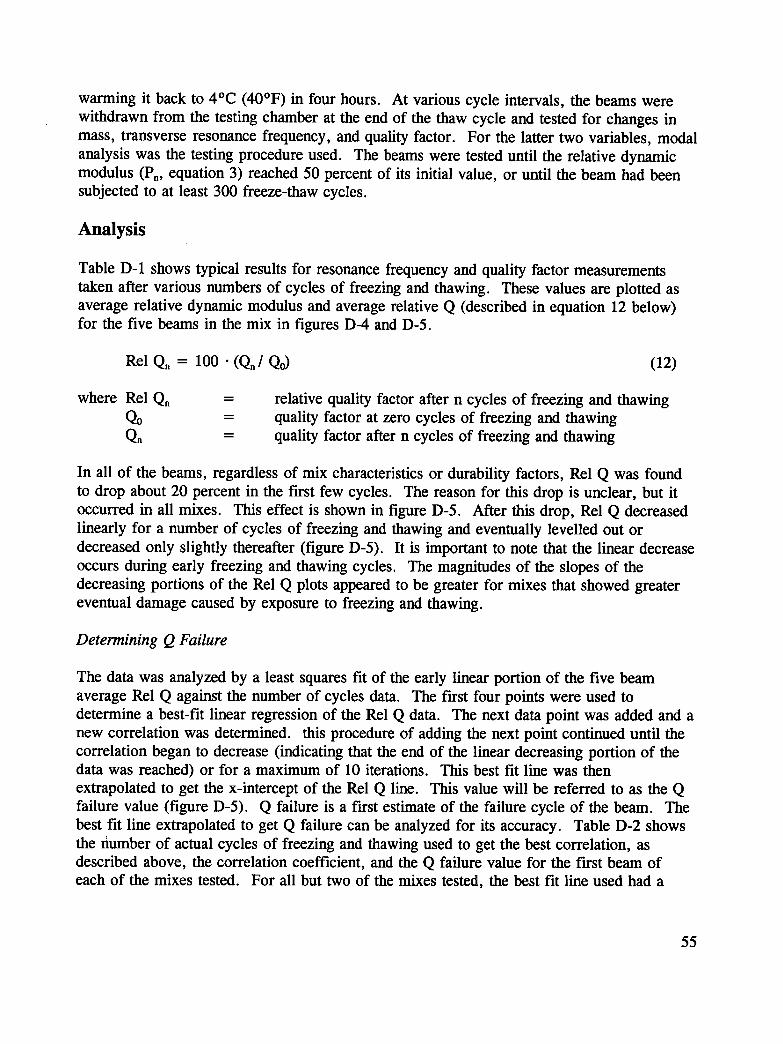
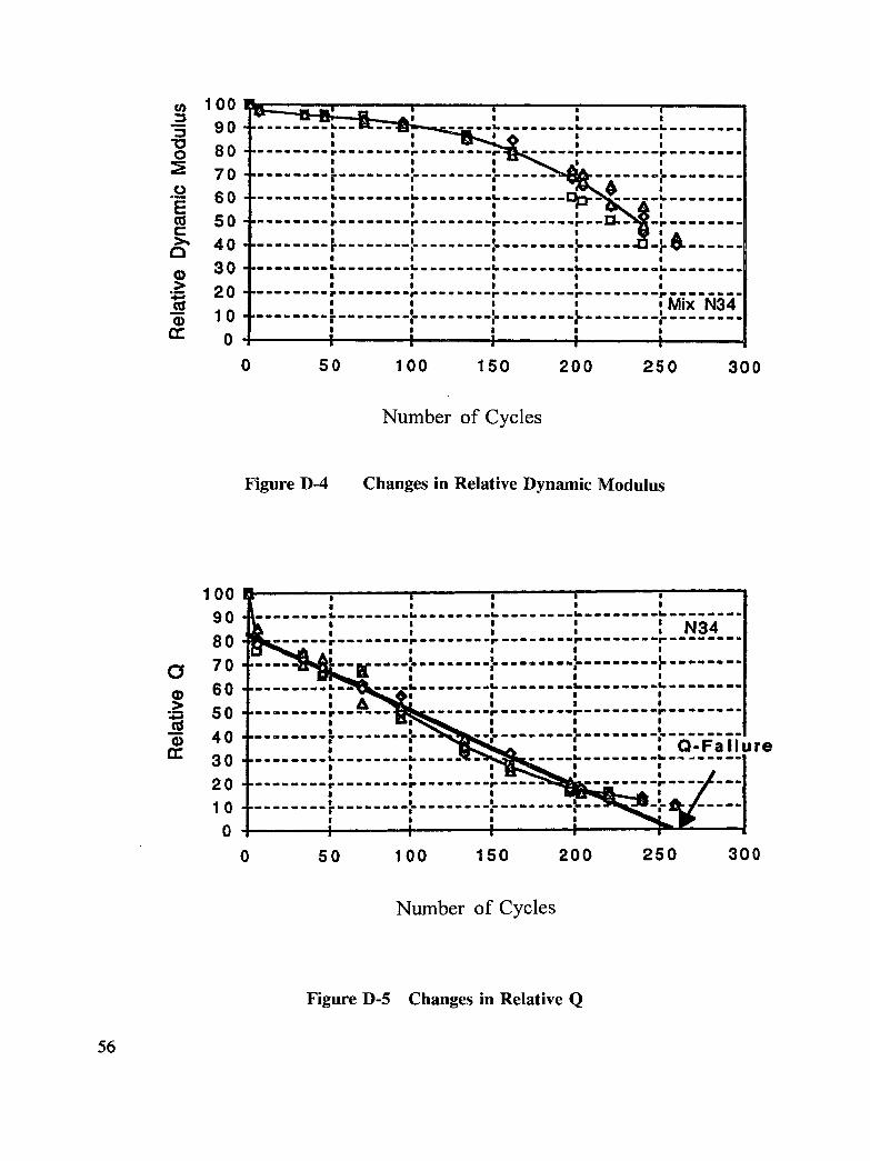
Figure D-4 Changes in Relative Dynamic Modulus ...................... 56
Figure D-5 Changes in Relative Q ................................ 56
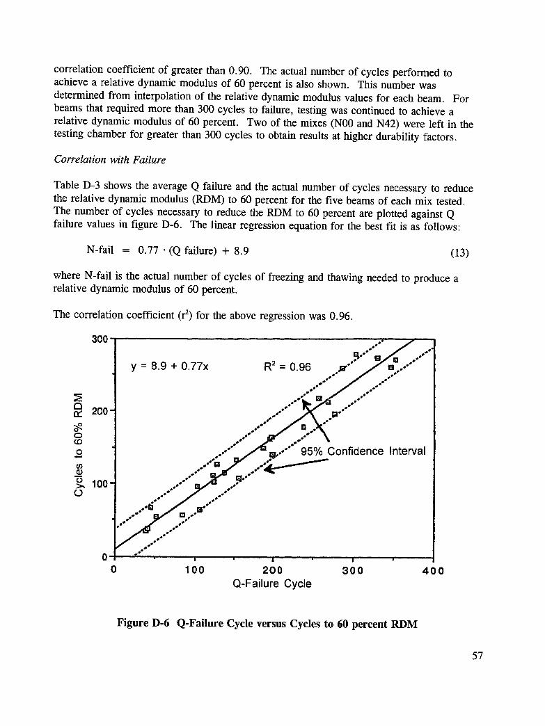
Figure D-6 Q-Failure Cycle versus Cycles to 60 percent RDM ............... 57
Part II
Figure 2-1 Winslow Absorption Rates for Four Aggregates ................. 88
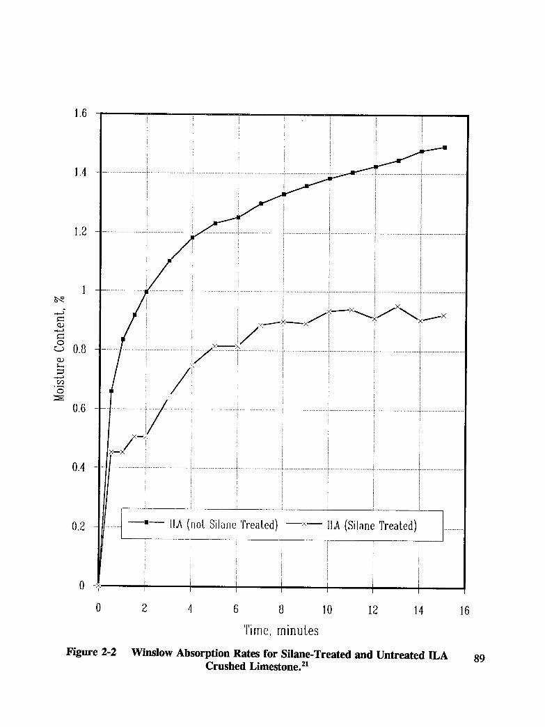
Figure 2-2 Winslow Absorption Rates for Silane-Treatedand ILA Crashed Limestone ............................. 89
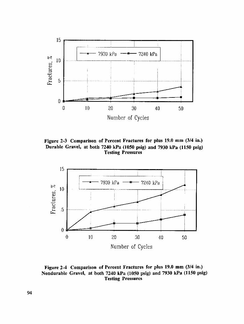
Figure 2-3 Comparison of Percent Fractures for plus 19.0 mm (3/4 in.)Durable Gravel, at both 7240 kPa (1050 psi)and 7930 kPa (1150 psi) Testing Pressures .................... 94
oo.
XIII
Figure 2-4 Comparison of Percent Fractures for plus 19.0 mm (3/4 in.)Nondurable Gravel, at both 7240 kPa (1050 psi)and 7930 kPa (1150 psi) Testing Pressures .................... 94
Figure 2-5 Comparison of Percent Fractures for plus 19.0 mm (3/4 in.)and minus 19.0 mm Durable Gravel ........................ 98
Figure 2-6 Comparison of Percent Fractures for plus 19.0 mm (3/4 in.)and minus 19.0 mm Nondurable Gravel ...................... 98
Figure 2-7 Pressure Release Rate History for Original Chamber .............. 99
Figure 2-8 Pressure Release Histories for Original and Large Chambers ........ 100
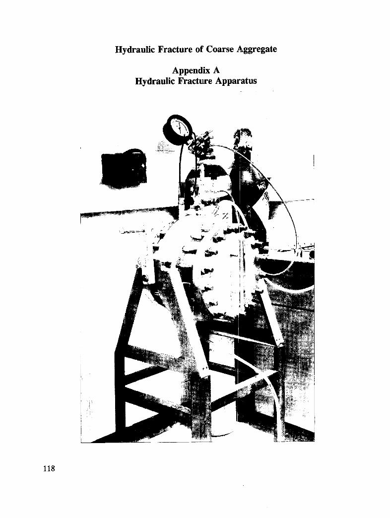
Figure 2-9 The Large Washington Hydraulic Fracture Test Apparatus ......... 101
xiv
List of Tables
Part I
Table 1-1 Relative Humidity at 25°C for Selected Saturated Salt Solutions ......... 4
Table 1-2 Summary of Rapid Test Method Comparisons .................... 7
Table 1-3 Comparison of Precision between ASTM C215
and the "Proposed Fundamental Transverse Frequencyand Quality Factor of Concrete Prism Specimens" ................. 9
Table 1-4 Comparison of DF Variability for Two Methodsof Measuring Fundamental Transverse Frequency .................. 9
Table A-1 Preliminary Tests for Statistical Calibrationand Normal Concretes (Matrix A) .......................... 19
Table A-2 Water Reducer and Air-Entraining Admixture Type (Matrix B) ........ 19
Table A-3 Cement and Aggregate Types,including SHRP C-205 HES Mixes (Method C) .................. 20
Table A-5 Pozzolan Amount and Curing Period (Matrix E) .................. 21
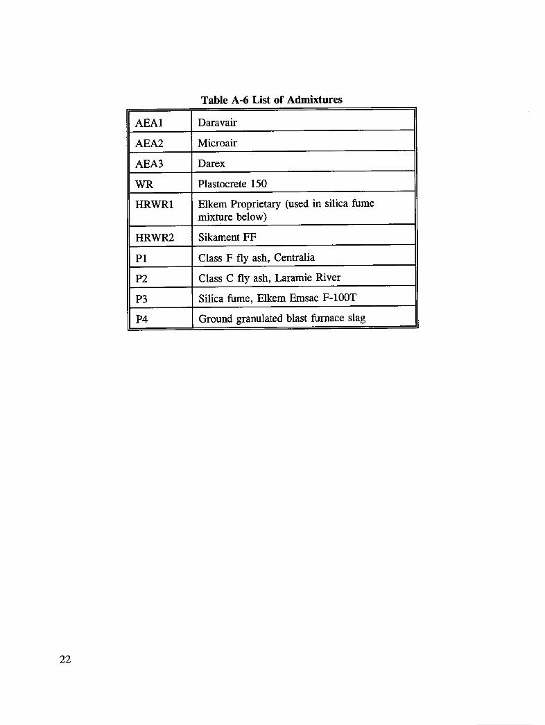
Table A-6 List of Admixtures .................................... 22
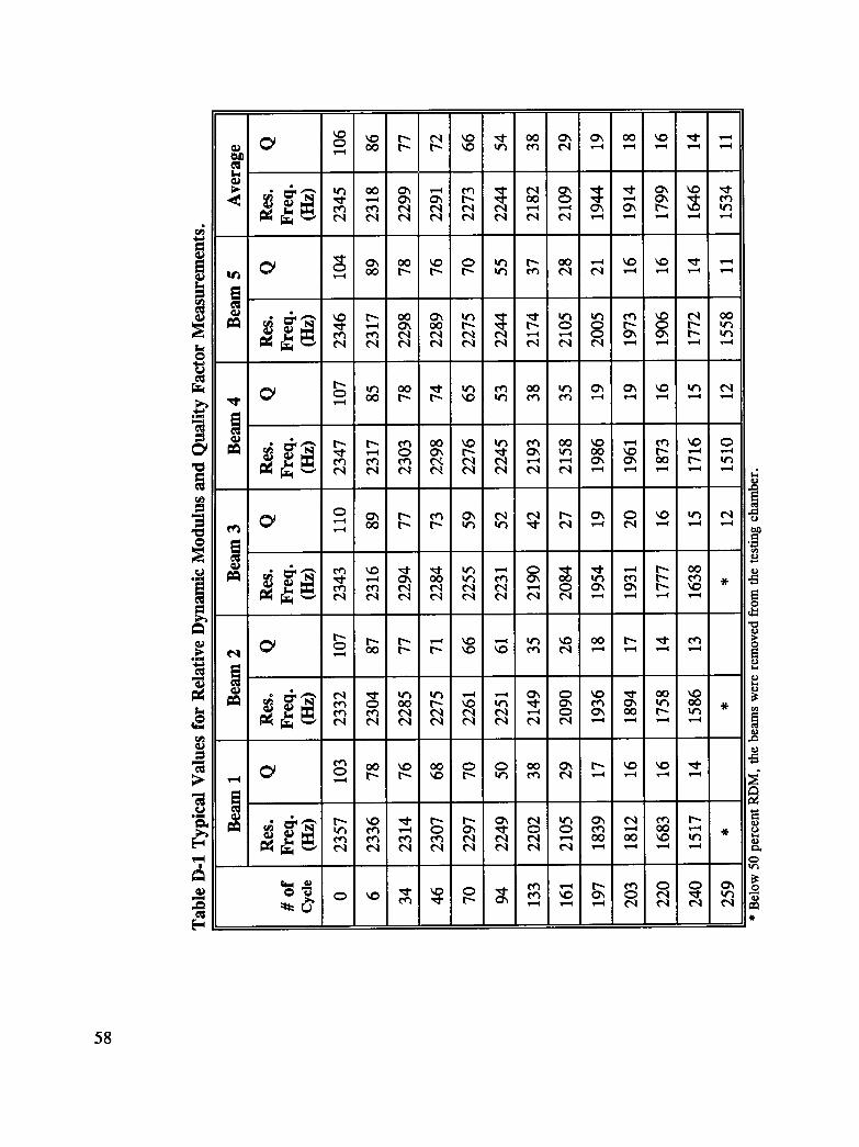
Table D-1 Typical Value for Relative Dynamic Modulusand Quality Factor Measurements ........................... 58
Table D-2 Q-Failure and Actual Failure Cycle, Single Beam from Each Mix Tested . . 59
Table D-3 Q-Failure and Cycles to 60 Percent RDM,Average of Five Beams from Each Mix Tested .................. 60
XV
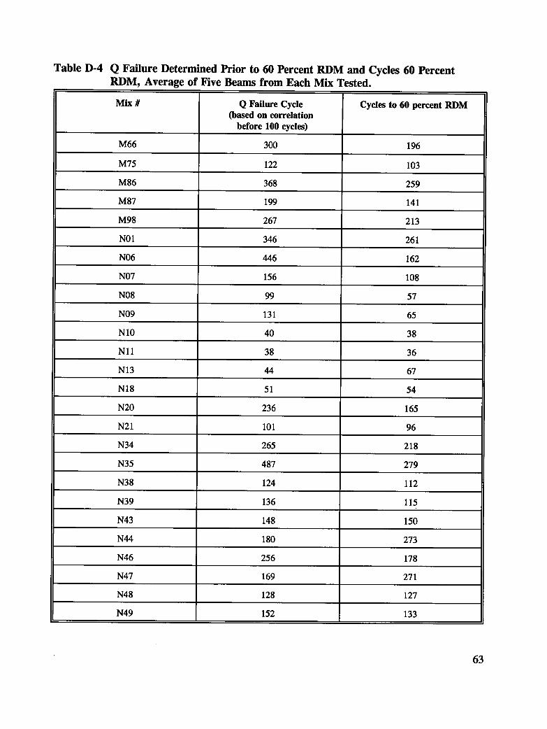
Table D-4 Q-Failure Determined Prior to 60 Percent RDMand Cycles 60 Percent RDM, Average of Five Beamsfrom Each Mix Tested ................................. 63
Table D-5 Predicted and Actual Durability Factors ....................... 64
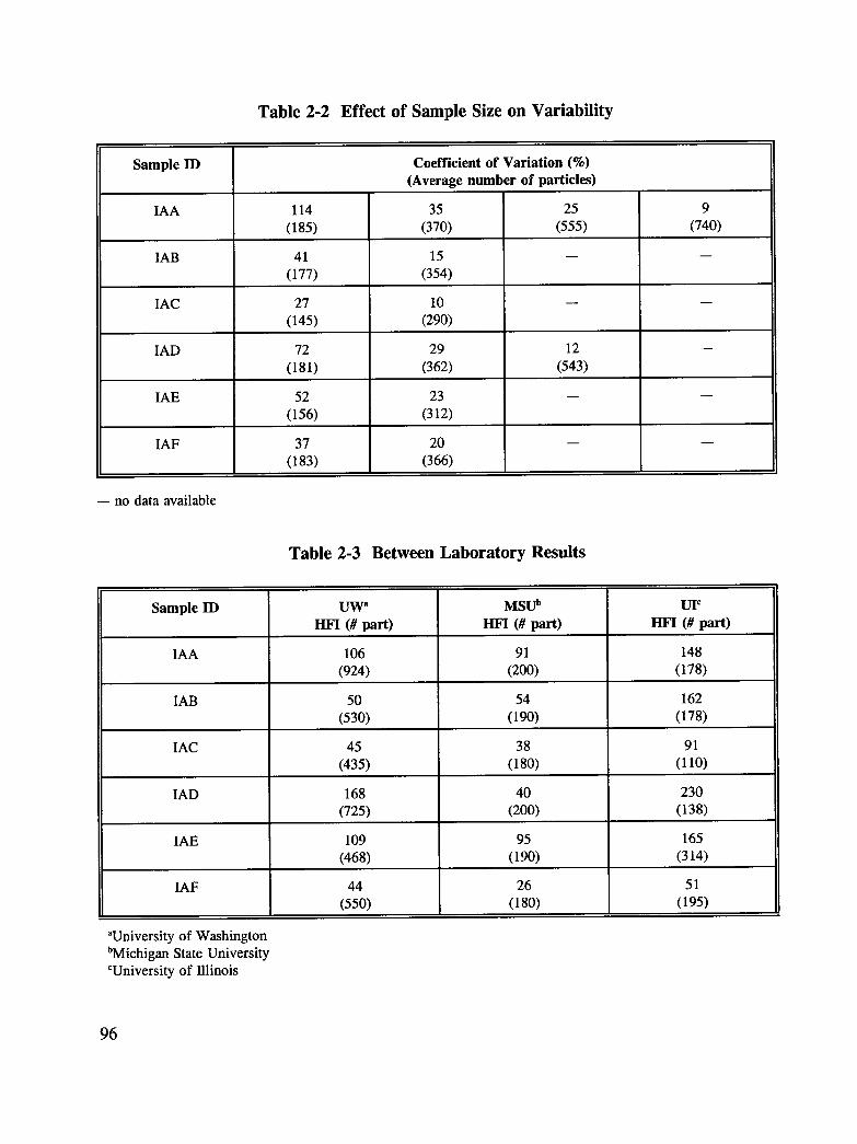
Table 2-2 Effect of Sample Size on Variability ......................... 96
Table 2-3 Between Laboratory Results .............................. 96
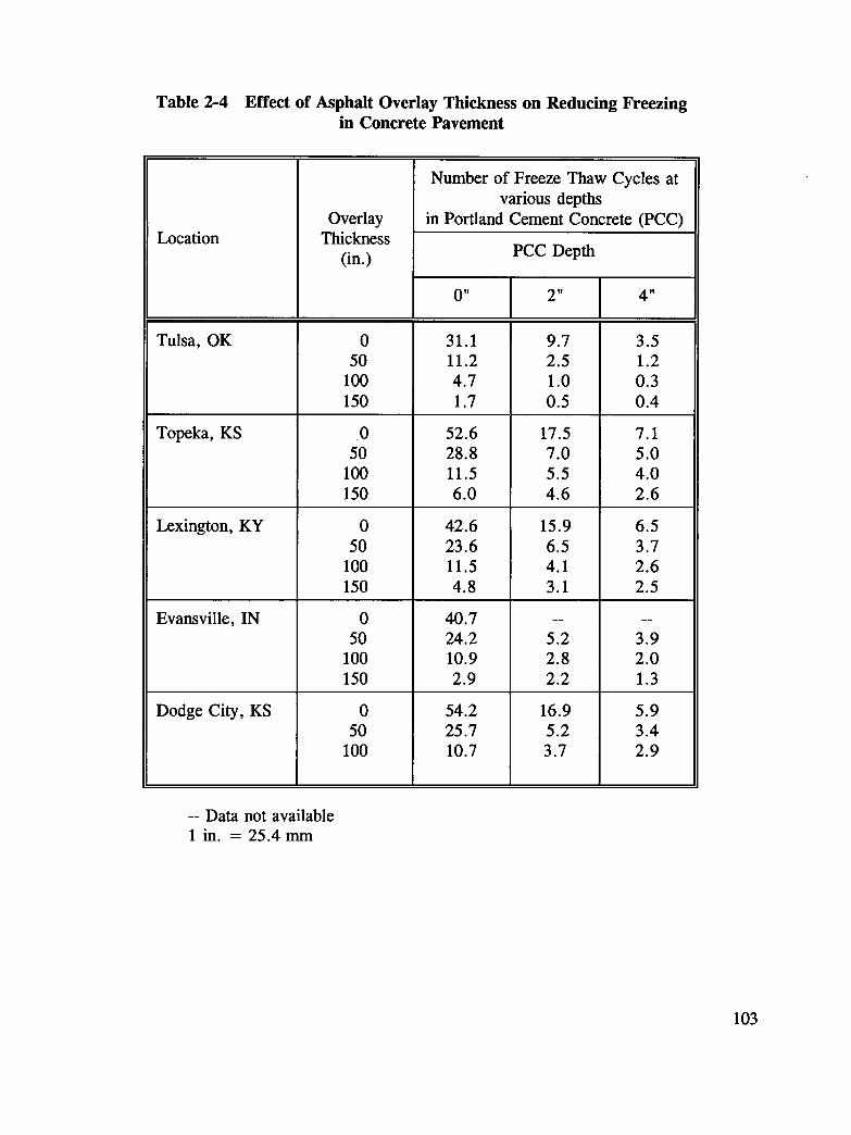
Table 2-4 Effect of Asphalt Overlay Thickness on Reducing Freezingin Concrete Pavement ................................. 103
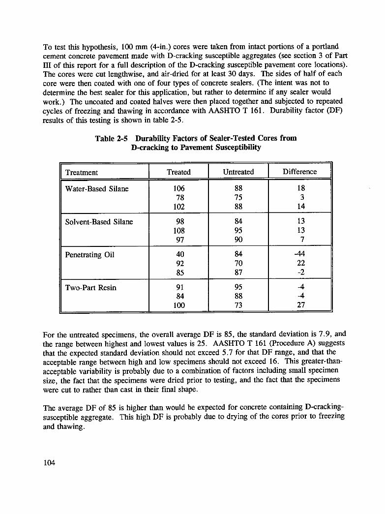
Table 2-5 Durability Factors of Sealer Tested Coresfrom D-Cracking to Pavement Susceptibility ................... 104
Part Ill
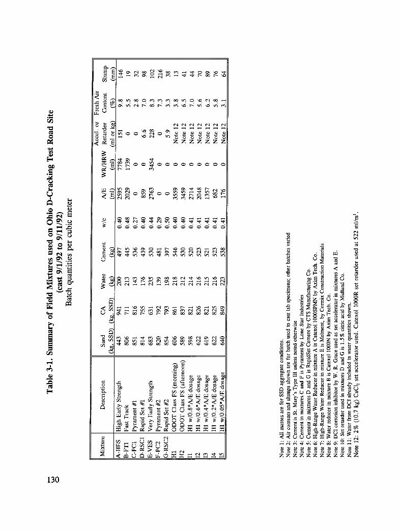
Table 3-1 Summary of Field Mixtures used on Ohio D-CrackingTest Road Site (Cast 9/1/92 to 9/11/92) ...................... 130
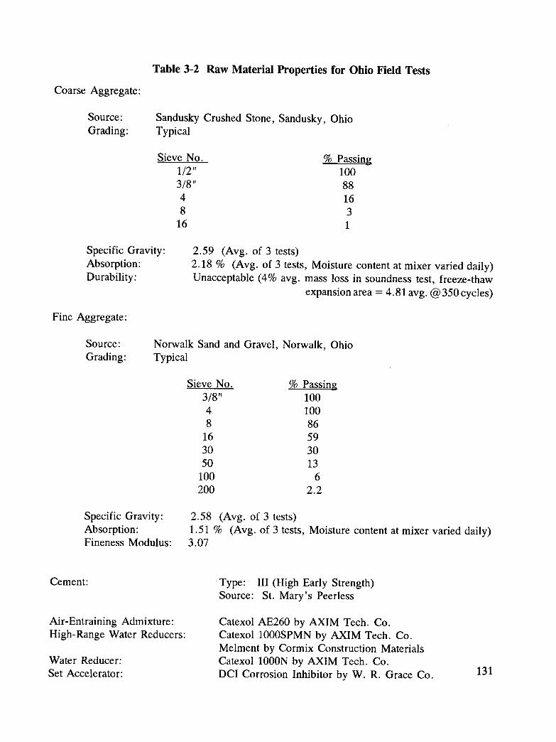
Table 3-2 Raw Material Properties for Ohio Field Tests .................. 131
Table 3-3 Layout of SHRP Concrete Frost Resistance Program Repairsand Concrete Sealers in Ohio ............................ 132
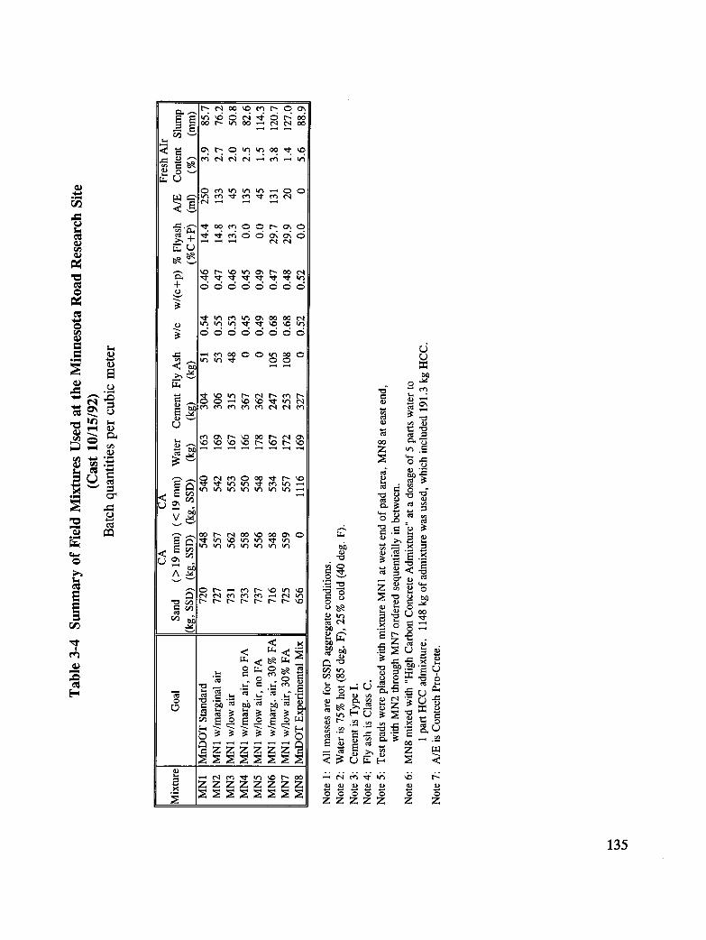
Table 3-4 Summary of Field Mixtures used at the Minnesota Road Research Site(Cast 10/15/92) ..................................... 135
Table 3-5 Raw Material Properties for Minnesota Field Tests ............... 136
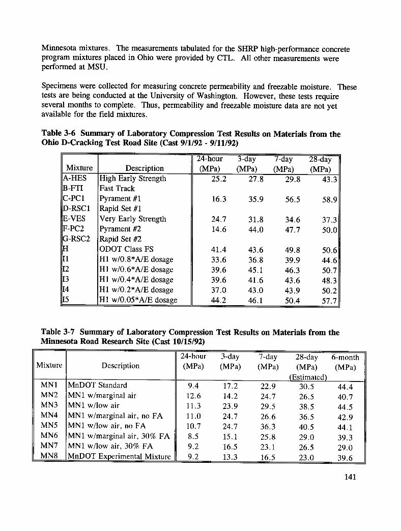
Table 3-6 Summary of Laboratory Compression Test Resultson the Materials from the Ohio D-Cracking Test Road Site(Cast 9/1/92 to 9/11/92) ............................... 141
Table 3-7 Summary of Laboratory Compression Test Resultson Materials from the Minnesota Road Research Site (Cast 10/15/92) .... 141
Table 3-8 Summary of Laboratory Durability Test ResultsOhio D-Cracking Test Road Site (Cast 9/1/92 to 9/11/92) ........... 142
xvi
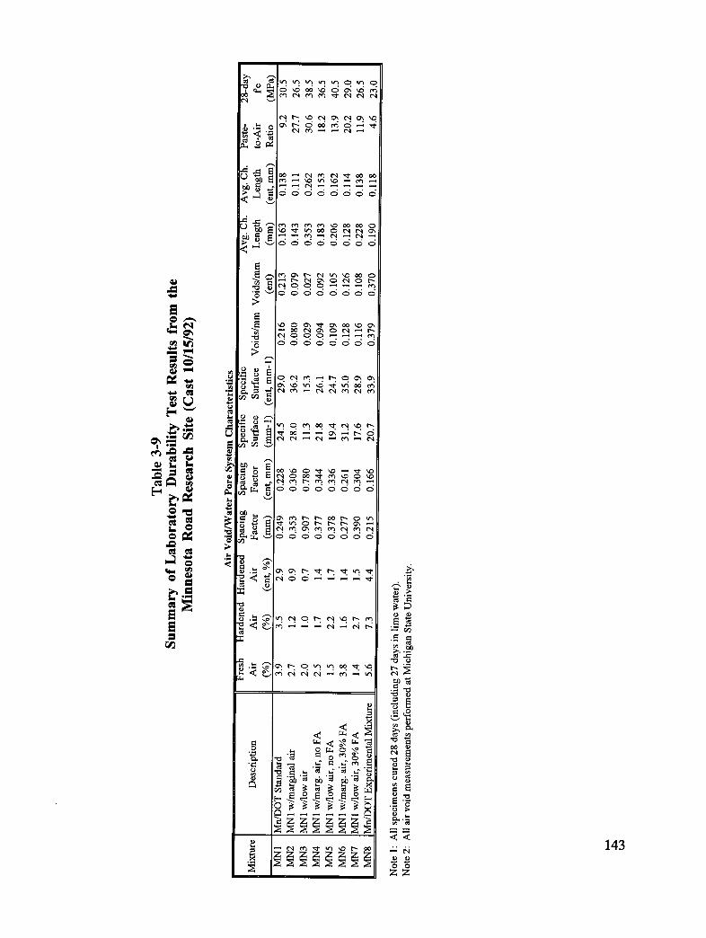
Table 3-9 Summary of Laboratory Durability Test Resultsfrom the Minnesota Road Research Site (Cast 10/15/92) ............ 143
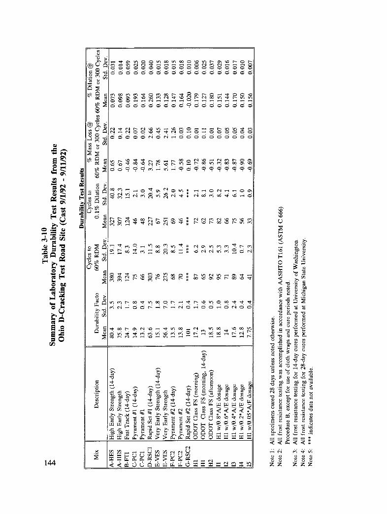
Table 3-10 Summary of Laboratory Durability Test Results
from the Ohio D-Cracking Test Road Site (Cast 9/1/92 to 9/11/92) ..... 144
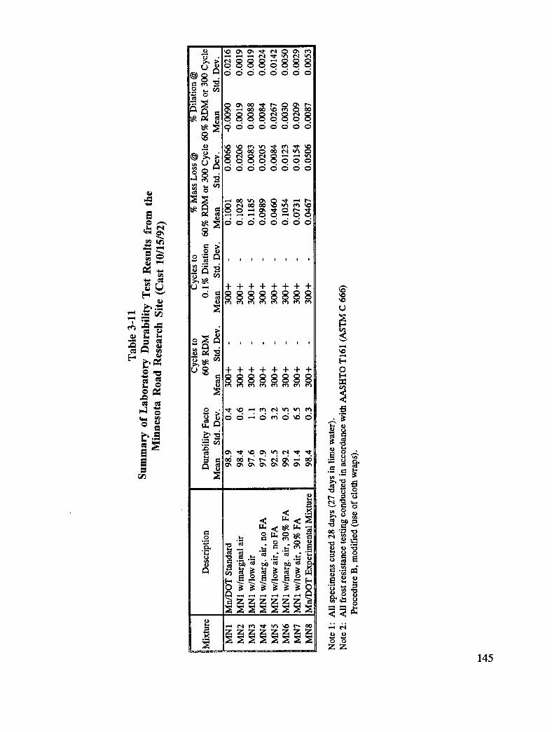
Table 3-11 Summary of Laboratory Durability Test Resultsfrom the Minnesota Road Research Site (Cast 10/15/92) ............ 145
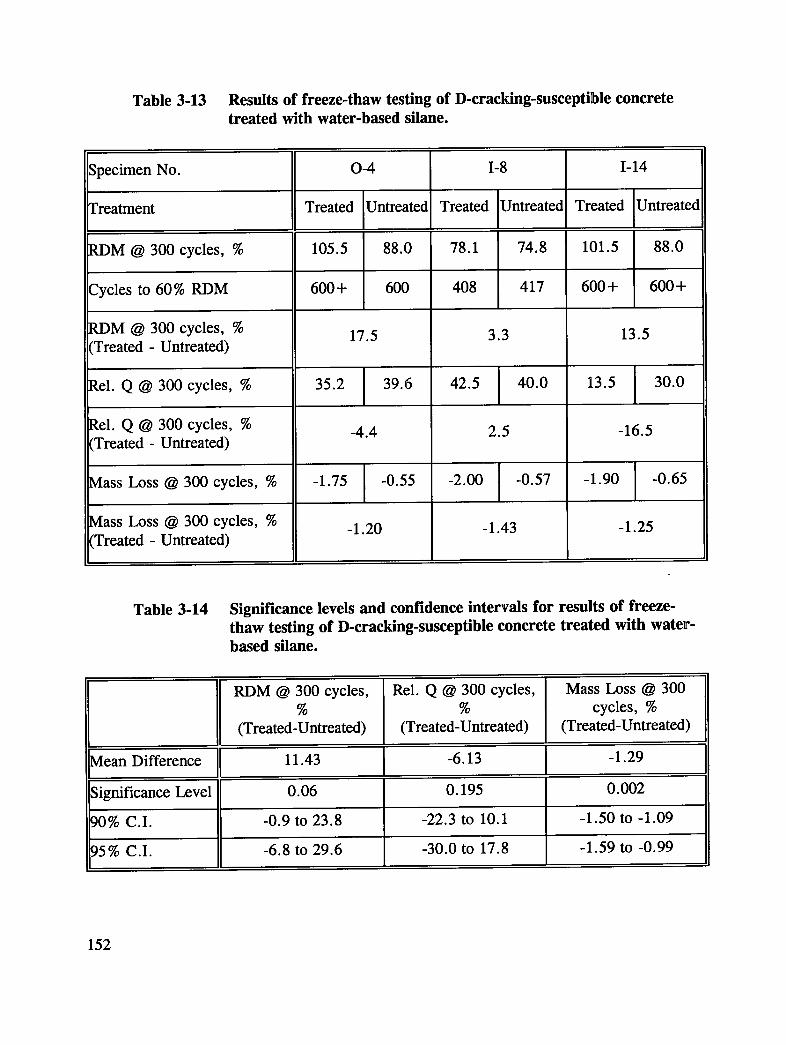
Table 3-13 Results of Freeze-Thaw Testing ofD-Cracking Susceptible Concrete Treated with Water-based Silane ..... 152
Table 3-14 Significance Levels and Confidence Intervals
for Results of Freeze-Thaw Testing of D-CrackingSusceptible Concrete Treated with Water-based Silane ............. 152
Table 3-15 Results of Freeze-Thaw Testing of D-CrackingSusceptible Concrete Treated with Solvent-based Silane ............ 154
Table 3-16 Significance Levels and Confidence Intervals for Resultsof Freeze-Thaw Testing of D-Cracking Susceptible ConcreteTreated with Solvent-based Silane ......................... 154
Table 3-17 Results of Freeze-Thaw Testing of D-CrackingSusceptible Concrete Treated with Penetrating Oil Sealer ........... 156
Table 3-18 Significance Levels and Confidence Intervals for Results
of Freeze-Thaw Testing of D-Cracking Susceptible ConcreteTreated with Penetrating Oil Sealer ......................... 156
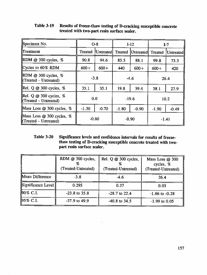
Table 3-19 Results of Freeze-Thaw Testing of D-CrackingSusceptible Concrete Treated with Two-Part Resin Surface Sealer ...... 157
Table 3-20 Significance Levels and Confidence Intervals for Resultsof Freeze-Thaw Testing of D-Cracking Susceptible ConcreteTreated with Two-Part Resin Surface Sealer ................... 157
xvii
Abstract
This study, aimed at improving the freeze-thaw resistance of concrete, consists of three parts.Part I evaluates parameters affecting the freeze-thaw durability of concrete. A modificationof the existing standard of method for determining the durability factor of concrete specimensis proposed, and a new procedure for fundamental transverse frequency (used in durabilityfactor calculations) has been developed. Part II focuses on developing better methods foridentifying nondurable aggregates, and has resulted in a rapid new test based on the hydraulicfracture of aggregates. Part III describes field experiments to evaluate the freeze-thawresistance of a number of specified concrete mixes and the use of sealants to mitigate D-cracking. Preliminary field performance results are presented.
xix
Executive Summary
This document summarizes the results of a four-year program of research into the resistanceof concrete to freezing and thawing. The work is presented in three parts. Part I is adiscussion of factors primarily relating to the paste portion of the concrete. Part II relatesprimarily to the coarse aggregate portion of the concrete. Part III summarizes preliminaryresults for the field work relating to Parts I and II. The appendices contain the data andother information supplemental to the parts. These three parts are summarized below:
Part I: Frost Resistance of Concrete Made with Durable Aggregate
A revised test procedure and a new test procedure for concrete made with durable (frost-resistant) aggregate by rapid freezing and thawing is presented. Durability factor (DF) wasmeasured for a variety of mix parameters, with the emphasis being placed on identifying mixcombinations that produced DF values in the 25 to 75 range. Air-void parameters weremeasured by linear traverse. The water pore systems were evaluated by permeabilitymeasurement and by determining the theoretical amount of water that would freeze at -18°C(called freezable moisture in the text).
A modification to AASHTO T 161 was developed to address concerns with current variationsof AASHTO T 161 regarding container restraint in Procedure A and specimen drying inProcedure B. The modification consists of wrapping the specimens in terrycloth to keepthem moist during freezing without needing containers. The modification is slightly moresevere than current procedures, and shows less variability in results.
A new procedure for determining fundamental transverse frequency (used to calculate DF)was developed. The procedure consists of causing a specimen to vibrate by impacting it withan instrumented hammer, then evaluating the frequency response spectrum measured with anaccelerometer. The procedure is more than an order of magnitude more precise than thepublished precision for the current method of determining fundamental transverse frequency,ASTM C 215. No frost resistance models were developed because insufficient freezablemoisture data was available to permit adequate modelling.
Part II: Frost Resistance of Concrete Made with Frost-SusceptibleAggregate
The primary focus of this part was to develop a new test procedure for identifying aggregateswhich are not durable when subjected to freezing and thawing in concrete (D-cracking
xxi
susceptible). The procedure, called the Washington Hydraulic Fracture Test, usescompressed gas to force water into the pores of a dry aggregate. When the pressure isreleased, the aggregate must dissipate internal pressure. Aggregate that cannot dissipate thepressure rapidly fracture. The amount of fracturing is determined, and a value called thehydraulic fracture index (HFI) is calculated. This value is an estimate of the number ofpressurization cycles necessary to produce 10 percent of the pieces of aggregate to fracture.The laboratory results were compared to reports of field performances. Aggregates withhigh (80 to 100 or higher) HFI values tended to be non-D-cracking susceptible, whileaggregates with low (less than about 60) HFI values tended to be D-cracking susceptible.
Mitigation for existing D-cracking was also investigated. Findings suggested that the mostsuitable method of treating existing D-cracked pavements would be to replace the concretewith a full-depth patch. Prior to placing the new concrete, the exposed face of the existingconcrete section should be sealed to prevent moisture intrusion. This method would only beappropriate for pavements and other concrete with considerable intact concrete away fromjoints and cracks. This mitigation method is evaluated in Part III.
Part III: Field Studies
Several questions arose from the work reported in Parts I and II of this report relating tofield performance, namely: 1) how the newly-developed modification of AASHTO T 161relates to field performance; 2) whether non-traditional mixes (such as mixes containingpozzolans or very high cement contents) follow the same accepted criteria for resistance tofreezing and thawing as traditional air-entrained mixes; and 3) whether the progression offield D-cracking can be slowed sufficiently to significantly extend the life of pavementscontaining D-cracking susceptible aggregates. These questions were addressed by theconstruction of field test sections.
Full-depth concrete patches made with a range of high-performance materials (high cementcontents, accelerators, and blended cements used to achieve specified early-openingstrengths) were placed. The concrete patches had a range of air contents to produce anexpected range of performance. Companion specimens from many of the mixes producedlaboratory DF values less than 60, and would be expected to fail. These test patches requirefurther monitoring to evaluate field performance.
Test slabs containing varying amounts of fly ash were placed in Minnesota with a range ofair contents to produce an expected range of performance. Companion specimens from mostof the mixes produced DF values above 90, even though the air-void systems would bejudged to be substandard by conventional wisdom. Further field monitoring will be neededto evaluate field performance of these sections. Many of the patches in Ohio were placed inpavements made with aggregates susceptible to D-cracking. Prior to placing the newconcrete, the cut faces of the existing concrete received one of a variety of sealer treatments.Field monitoring will be needed to evaluate differences in field performance of the sealertreatments.
xxii
Part I - Frost Resistance of Concrete Made with DurableAggregate
1.0 Introduction
1.1 Background
Frost resistance of concrete made with durable aggregate is determined by the air-voidsystem's ability to prevent development of destructive pressures due to freezing andassociated movement of moisture in the concrete pores. The specific requirements of theair-void system depend on the amount and mobility of the water in the pores. Aninvestigation of the frost resistance of concrete made with durable aggregates should identifythe air-void system necessary to protect a variety of concrete water-pore systems.
1.2 Objectives
The goal of this research was to determine the effects of water-cement (w/c) andwater-cementitious [w/(c+p)] ratios, various air-entraining admixtures, water-reducing andhigh-range water reducing admixtures, pozzolanic iidmixtures, and ground granulated blastfurnace slag on the frost resistance of concrete made with durable aggregates. Frostresistance was evaluated by rapid laboratory testing. Field evaluation of selected mixes isdiscussed in Part III.
In particular, the research examined1. procedures for rapid freezing and thawing testing with modifications to these
procedures if appropriate;2. procedures for nondestructive evaluation of damage from rapid freezing and
thawing. Procedure modifications were made if deemed appropriate;3. various methods of quantifying the air-void system in hardened concrete;4. methods of evaluating the water pore system in hardened concrete;5. combination of the air-void and water pore systems to better predict resistance
to freezing and thawing.
2.0 Laboratory Testing Program
2.1 Purpose
The laboratory testing program developed a data set. Because the amount of testingnecessary to define durability factor (DF) versus air-void parameter relations for the range of
mix parameters of interest would be prohibitive, an alternate approach was used. Manyresearchers have shown that this relationship is relatively linear for the midrange of DFvalues (approximately 25 to 75). 1 Therefore, the initial testing defined the slope of thislinear range for base mixes made with 0.40 and 0.45 w/o's. Assuming that these slopes heldfor other mix combinations with the same w/c values, testing of other mix combinationswould concentrate on mixes with marginal DF values in this 25-to-75 range.
This approach required considerable attention to the minimization of testing errors. Thisinvolved repeated freezing and thawing testing, along with nondestructive evaluation ofspecimen deterioration. Chapter 3 descibes the innovative test procedures used.
2.2 Test Matrices
Test matrices were developed that combined the various parameters of:
Parameter Variable
w/c 0.40, 0.45, 0.52
Cement Type Type I, Type II, Type III
Air-Entrainment Admixture vinsol resin, two other proprietary(AEA) AEA's
Water Reducing (WR) and one WR and two HRWR'sHigh-Range Water Reducing(HRWR) Admixtures
Pozzolan Types one Class C flyash, one Class Fflyash, one silica fume, and oneground granulated blast furnace slag
w/(c+p) 0.40, 0.45 (w/c's of 0.45, 0.46, 0.52and 0.59, depending upon pozzolancontent)
Coarse Aggregate crushed limestone and glacial gravel
Curing 14, 28 (std.) and 56 days in limewater
Specialty High-Performance very early strength and high earlyMixes strength mixes, Pyrament, Rapid Set
cement
The design matrices showing the various combinations of the above parameters are presentedin appendix A.
2
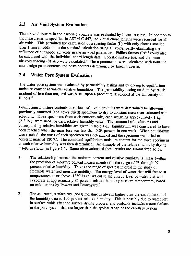
2.3 Air Void System Evaluation
The air-void system in the hardened concrete was evaluated by linear traverse. In addition tothe measurements specified in ASTM C 457, individual chord lengths were recorded for allair voids. This permitted the calculation of a spacing factor (I_,)with only chords smallerthan 1 mm in addition to the standard calculation using all voids, partly eliminating theinfluence of entrapped air voids in the air-void parameter. Philleo factors (p)2.3 could alsobe calculated with the individual chord length data. Specific surface (or), and the meanair-void spacing (S) also were calculated. 4 These parameters were calculated with both themix design paste contents and paste contents determined by linear traverse.
2.4 Water Pore System Evaluation
The water pore system was evaluated by permeability testing and by drying to equilibriummoisture content at various relative humidities. The permeability testing used an hydraulicgradient of less than ten, and was based upon a procedure developed at the University ofIllinois. 5
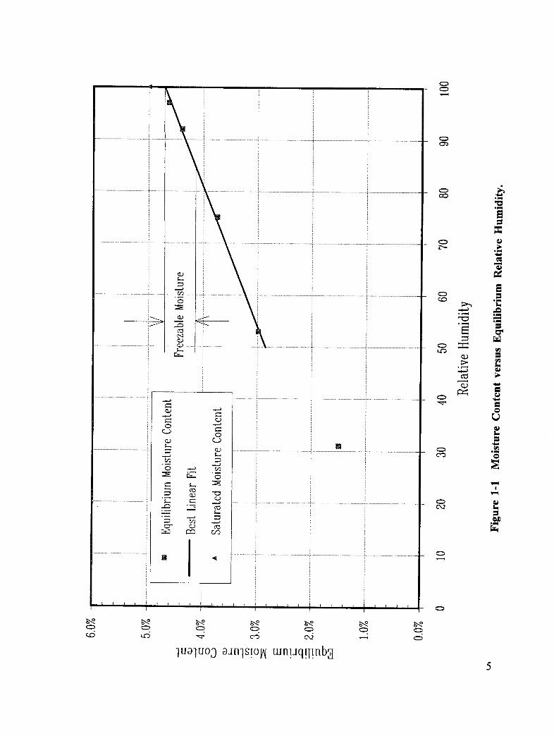
Equilibrium moisture contents at various relative humidities were determined by allowingpreviously saturated (and never dried) specimens to dry to constant mass over saturated saltsolutions. Three specimens from each concrete mix, each weighing approximately 1 kg(2.2 lb.), were used for each relative humidity value. The saturated salt solutions andcorresponding relative humidities are given in table 1-1. Equilibrium was considered to havebeen reached when the mass loss was less than 0.03 percent in one week. When equilibriumwas reached, the mass of each specimen was determined and the specimen was dried toconstant mass at 120°C. The combined equilibrium moisture content for the three specimensat each relative humidity was then determined. An example of the relative humidity dryingresults is shown in figure 1-1. Some observations of these results are summarized below:
1. The relationship between the moisture content and relative humidity is linear (withinthe precision of moisture content measurements) for the range of 53 through 97percent relative humidity. This is the range of greatest interest in the study offreezable water and moisture mobility. The energy level of water that will freeze attemperatures at or above -18°C is equivalent to the energy level of water that willevaporate at approximately 85 percent relative humidity at room temperature, basedon calculations by Powers and Brownyard. 6
2. The saturated, surface-dry (SSD) moisture is always higher than the extrapolation ofthe humidity data to 100 percent relative humidity. This is possibly due to water leftin surface voids after the surface drying process, and probably includes macro-defectsin the pore system that are larger than the typical range of the capillary system.
Table 1-1 Relative Humidity at 25°C for Selected Saturated Salt Solutions.
Saturated Salt Solution Relative Humidity %
K2SO4 97
KNO3 92
NaC1 75
Mg(N03)2" 6(H20 ) 53
CaC1E-6(H20 ) 31
3. The moisture content at 31 percent relative humidity is always below the best-fitstraight line portion of the data at higher humidities. While this relative humidityrange is below the range of interest for freezing in concrete (and the range that wouldbe considered a part of the capillary system), this data may be of interest in theinvestigation of concrete microstructure.
Two parameters are used to quantify the effects of water in the pore system: permeabilityand the freezable moisture. Because permeability applies only to a saturated material andconcrete is seldom completely saturated, permeability was considered of secondaryimportance in quantifying the water pore system. Freezable moisture is defined as theamount of moisture in the capillary system of the concrete that would theoretically freeze ator above -18°C. It is determined as the difference between moisture contents taken at 85
and 100 percent relative humidities on the linear portion of the moisture content-humidityrelationship shown in figure 1-1. This specifically excludes the moisture characterized asresiding in macrodefects in point 2 above. While the selection of -18°C as the referencetemperature for determining theoretical freezable moisture is based only upon the minimumtemperature reached during rapid freezing and thawing (AASHTO T 161), the linear natureof the moisture content-humidity relationship found for the concretes tested suggests thatselection of an alternate freezing temperature would simply apply a scaling factor to allfreezable moisture results reported in this work.
oo
2.5 Freezing and Thawing Test Procedure
There are a variety of testing procedures available to determine the resistance of concrete tofreezing and thawing. The most commonly used procedures in the United States areAASHTO T 161 (ASTM C 666), "Resistance of Concrete to Rapid Freezing and Thawing",and ASTM C 672, "Scaling Resistance of Concrete Surfaces Exposed to Deicing Chemicals".The latter procedure uses a qualitative evaluation of the amount of scaling produced. Resultsfrom this procedure would not be suitable for the statistical analysis used to evaluate theinfluence of the various mix parameters. Efforts to develop a quantitative scaling test wereunder way in Europe 7 concurrent with the testing summarized in this report. These effortshad not culminated in an acceptable procedure in time for the procedure to be considered inthis work.
AASHTO T 161 is the most commonly used laboratory method for the evaluation of theresistance of concrete to freezing and thawing in the United States. Most highway agenciesin freezing climates have access to equipment capable of performing this test. Despite (orperhaps because of) the popularity and availability of equipment for AASHTO T 161,considerable controversy exists over the appropriateness of using it to predict field durabilityand over limitations of the variations of the procedure. The first issue is addressed in PartIII of this report.
As for the second issue, AASHTO T 161 describes two primary variations for achieving thespecified freezing and thawing: Procedure A, Rapid Freezing and Thawing in Water; andProcedure B, Rapid Freezing in Air and Thawing in Water. Testing by Procedure Agenerally uses a container of some type that allows the specimen to be surrounded by "notless than 1/32 in. (1 mm) nor more than 1/8 in. (3 mm) of water at all times." Appropriatecautions are given concerning problems associated with rigid containers and the ice pressurethat can build up between the container wall and the specimen. In extreme cases, this icepressure can actually damage the specimens. In any case, the use of a container must resultin some amount of pressure on the specimen when the water surrounding the specimenfreezes. If the specimen is not perfectly centered in the container, differential pressures willdevelop due to the differences in thickness of the ice surrounding the specimen duringfreezing. An additional problem with the containers is maintaining the proper thickness ofsurrounding water for specimens that exhibit scaling. Containers that start with a waterthickness that is close to the maximum could exceed this thickness after some scaling of thespecimens. Containers with a water thickness closer to the minimum limit tend to bindagainst the specimens due to accumulation of scaled material in the lower portions of thecontainer. Removal of these bound specimens from their containers could result in physicaldamage to the specimens.
The primary objection to Procedure B is that the specimens are allowed to dry duringfreezing, which slows the accumulation of damage. Most refrigeration equipment cools airby circulating it past refrigerated coils and then over the test specimens. Moisture in the aircondenses on the coils. This dried, cooled air removes moisture from the specimens in
6
addition to removing heat. Many agencies compensate for this delayed accumulation ofdamage from drying by testing to a minimum of 350 cycles of freezing and thawing ratherthan 300, which is common for testing by Procedure A.
These problems with the standard variations of AASHTO T 161 were addressed by thedevelopment of a new variation which attempts to eliminate the perceived shortcomingsdescribed above. This new variation is addressed below.
3.0 Innovative Test Procedures
3.1 Modification of AASHTO T 161 (ASTM C 666)
A modification of AASHTO T 161 (ASTM C 666), Procedure B has been developed thatconsists of wrapping the specimens with absorbent cloth to keep the specimens wet duringfreezing. This modification is hereafter called Procedure C, and is in response to the majorcriticisms described above. Briefly, these criticisms are that in Procedure B, the specimensare allowed to dry during freezing, and that in Procedure A, the physical confinement ofspecimens by rigid specimen holders could cause damage, along with the problem ofmaintaining the correct thickness of water surrounding the specimens. A summary of themodifications to the published procedure for AASHTO T 161 is given in appendix B.
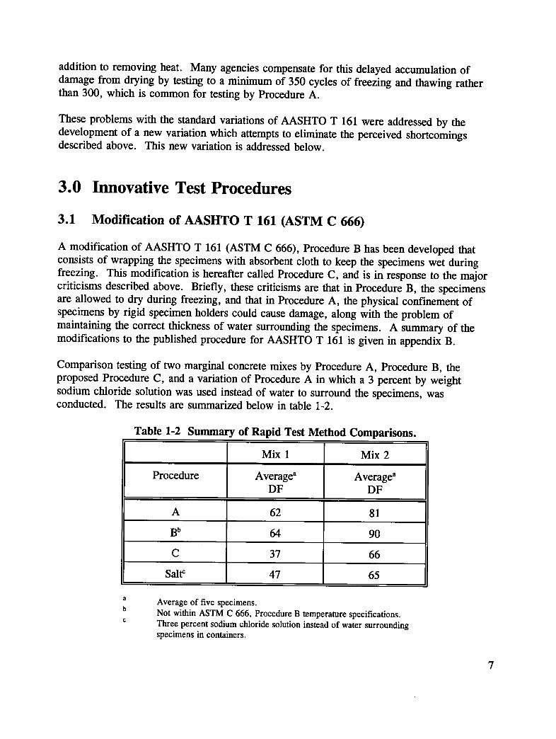
Comparison testing of two marginal concrete mixes by Procedure A, Procedure B, theproposed Procedure C, and a variation of Procedure A in which a 3 percent by weightsodium chloride solution was used instead of water to surround the specimens, wasconducted. The results are summarized below in table 1-2.
Table 1-2 Summary of Rapid Test Method Comparisons.
Mix 1 Mix 2
Procedure Average a AverageaDF DF
A 62 81
Bb 64 90
C 37 66
Salt¢ 47 65
a Average of five specimens.b Not within ASTM C 666, Procedure B temperature specifications.e Three percent sodium chloride solution instead of water surrounding
specimens in containers.
7
All of the testing took place simultaneously in a single test chamber. The procedures wereconducted in the following manner:
1. The containers for Procedure A and the salt solution were plastic rather than metal asused by most investigators. This probably reduced the detrimental effects of unequalice pressures often associated with the use of metal containers.
2. Procedure B was not within temperature specifications as the lack of any kind ofcovering permitted the specimen to cool below the specified 0°F+3°F.
3. Cooling rate was more uniform for Procedure C than for Procedure A. Procedure Ashowed a plateau in the 30-32°F range while the water surrounding the specimenfroze, followed by a more rapid drop in temperature. The cloth wrap in Procedure Cdid not hold sufficient water to produce a pronounced plateau, but probably did inhibitheat transfer from the wrapped specimen during the entire freezing period.
Though original expectations were that the severity of Procedure C would be between that ofProcedures A and B, the appearance is that the cloth wraps are slightly more severe thanProcedure A when container restraint effects are reduced.
3.2 Modification of ASTM C 215
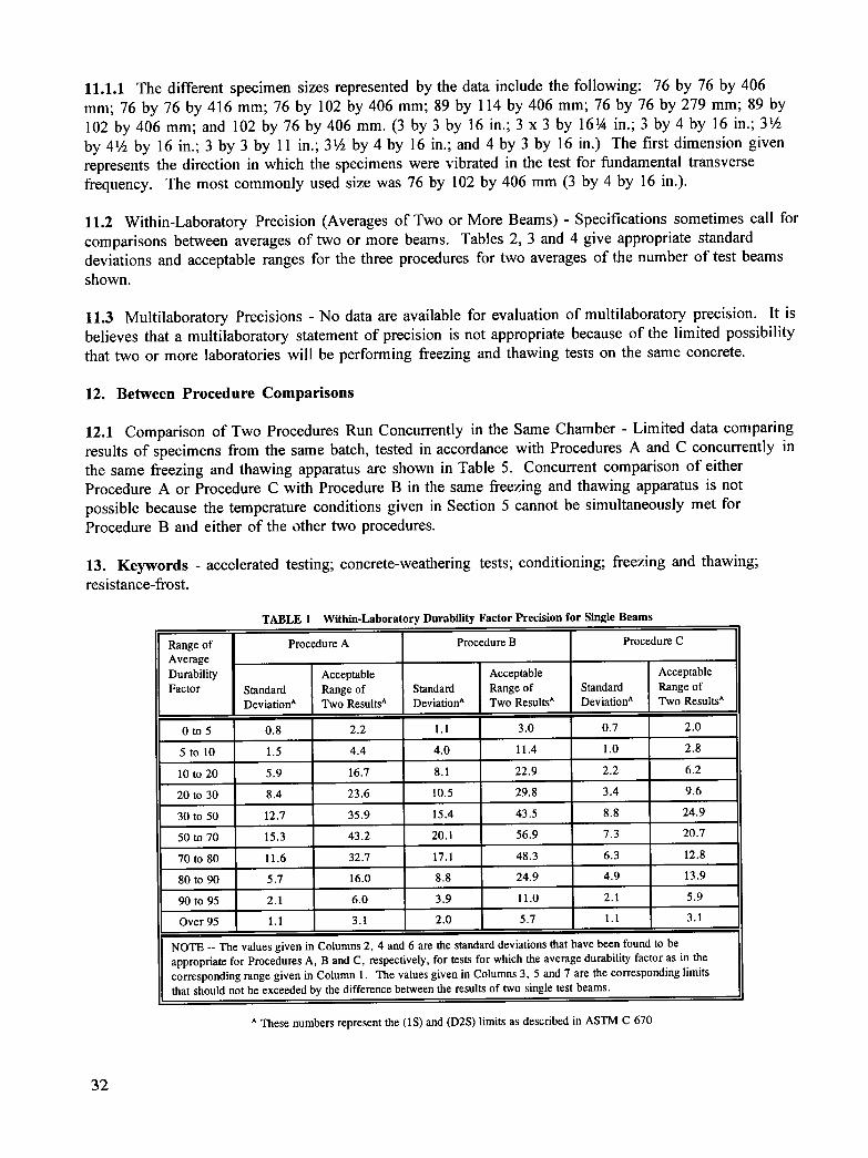
The relative dynamic modulus, as determined by resonance frequency measurements, is themost frequently used indicator for evaluating damage to concrete beams that are subjected torepeated cycles of freezing and thawing (AASHTO T 161). While sinusoidal excitation(ASTM C 215-85) has been the standard method for measuring resonance frequency, impulseexcitation (ASTM C 215-91) has recently been approved as an alternate. With minimalchanges in procedure from that specified in ASTM C 215, substantial improvements inprecision can be achieved. Also, quality factor Q, the inverse of the damping coefficient,can be determined with no additional testing. A proposed test method, FundamentalTransverse Frequency and Quality Factor of Concrete Prism Specimens, is included asappendix C.
The improvements in precision are shown in table 1-3. The acceptable range for thefundamental transverse frequency of an undamaged concrete beam is reduced by more thanan order of magnitude by the new procedure. While a similar comparison cannot be directlymade for specimens with substantial deterioration due to freezing and thawing, the relativeimprovement in precision would be expected to be about the same.
Experience has shown that the variability of DF results from AASHTO T 161 is dependentupon the actual DF value. Both high and low DFs have low variabilities, while intermediateDFs can have rather high variability. Mixes with intermediate DF values were determined tobe most significant in the freezing and thawing portion of this study as described in section2. The influence of this improvement in measurement precision of the fundamental
8
transverse frequency is shown in table 1-4. This table presents the average standarddeviation for groups of five specimens subjected to repeated cycles of freezing and thawingas in AASHTO T 161. The DF values for one set of specimens were determined bymeasurement of the fundamental transverse frequency determined by the forced vibrationmethod in accordance with ASTM C 215. The DF values for the second set of specimenswere determined by measurement of the fundamental transverse frequency using theprocedure given in appendix C.
Table 1-3 Comparison of Precision between ASTM C 215 and the Proposed"Fundamental Transverse Frequency and Quality Factor of
Concrete Prism Specimens"
Specimen Condition Acceptable Range of Two ResultsFundamental Transverse Frequency (%)_
ASTM C 215 New Procedure
Undamaged 2.8 0.11
Damaged b _c 0.51
° These numbers represent, respectively, the 1S% and D2S% limits as described in ASTM Practice C 670.bSpecimen was reduced by repeated cycles offreezing and thawing to approximately 60 percent relative
dynamic modulus as defined in Test Method T 161.c Not specifically given, though ASTM C 215 states both that "(the precision is)for concrete prisms as
originally cast. They do not necessarily apply to concrete prisms after they have been subjected to
freezing.and-thawing tests," and that " (the coefficient of variatlan has) been found to be relatively
constant ... for a range of specimen sizes and age or condition of the concrete, within limits."
Linear changes in damping with early cycles of freezing and thawing were found beforesignificant decreases in resonance frequency could be identified. Comparisons of predictedand actual durability factors show agreement within published testing errors for most of themixes tested. This work indicates that the durability factor (AASHTO T 161) can beaccurately predicted with damping measurements before the actual failure of the concretebeams because of repeated cycles of freezing and thawing. (See appendix D.)
Table 1-4 Comparison of DF Variability for Two Methods of MeasuringFundamental Transverse Frequency.
DF Range Standard Deviation Standard Deviation(ASTM C 215) (Appendix C)
20 to 30 4.2 3.0
30 to 50 9.8 4.5
50 to 70 8.0 5.4
9
4.0 ResuLts
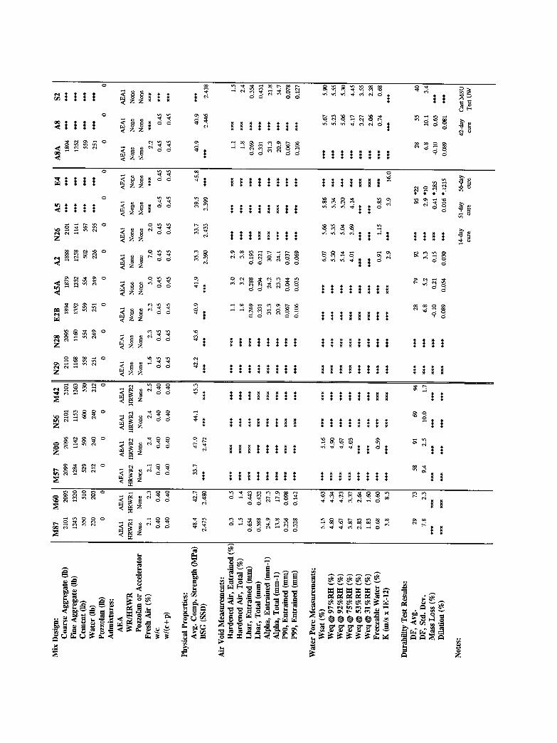
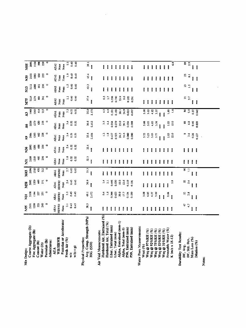
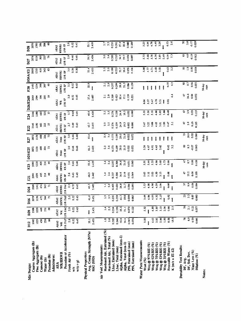
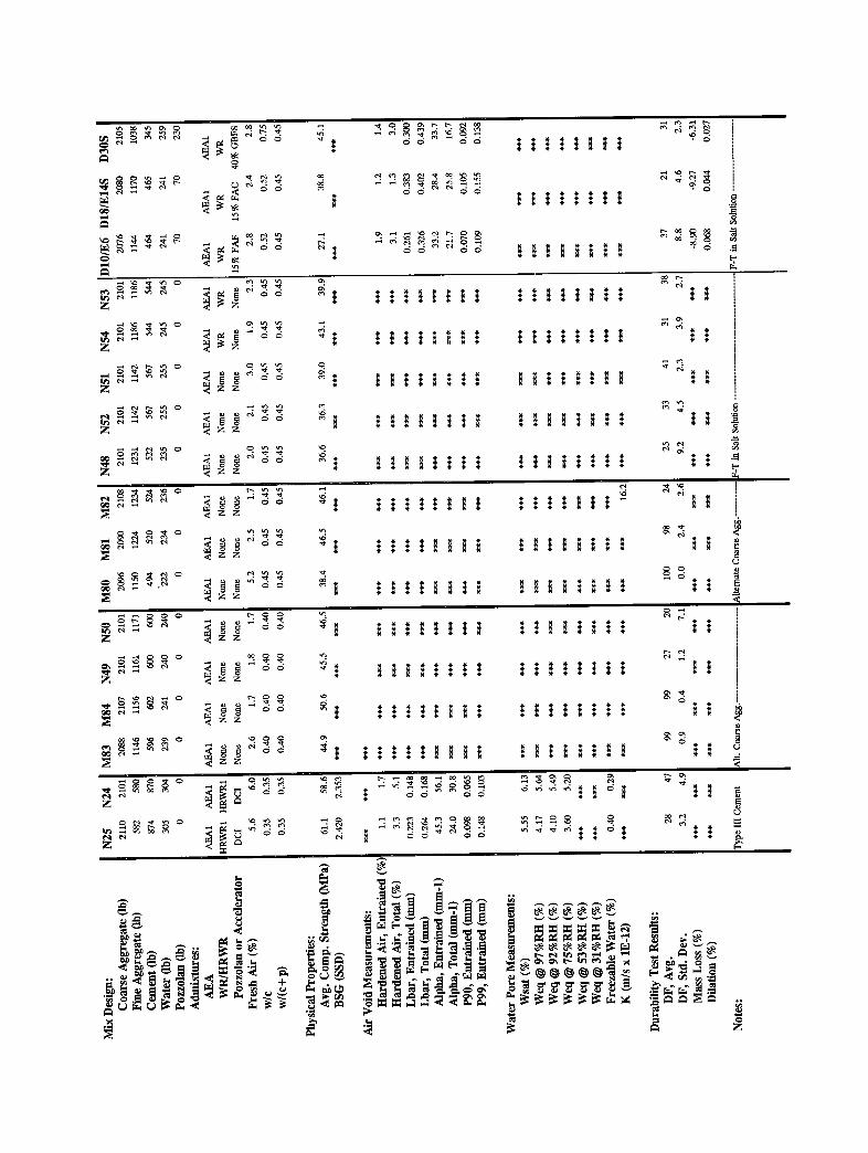
Tables of the results of the laboratory testing program are given in appendix E. Thisappendix includes mix design information, DF results, linear traverse results, andpermeability and freezable moisture results. Portions of the testing were not completed at thetime of the preparation of this report, most notably the freezable moisture values. These willbe made available as the testing is completed.
5.0 Acceptable Variability and Maximum Expected Errorsin Results
Prior to analysis of any results, the variability and maximum expected errors should bedetermined. These are discussed below for the various results obtained in this study.
5.1 Variability of Durability Factor Results
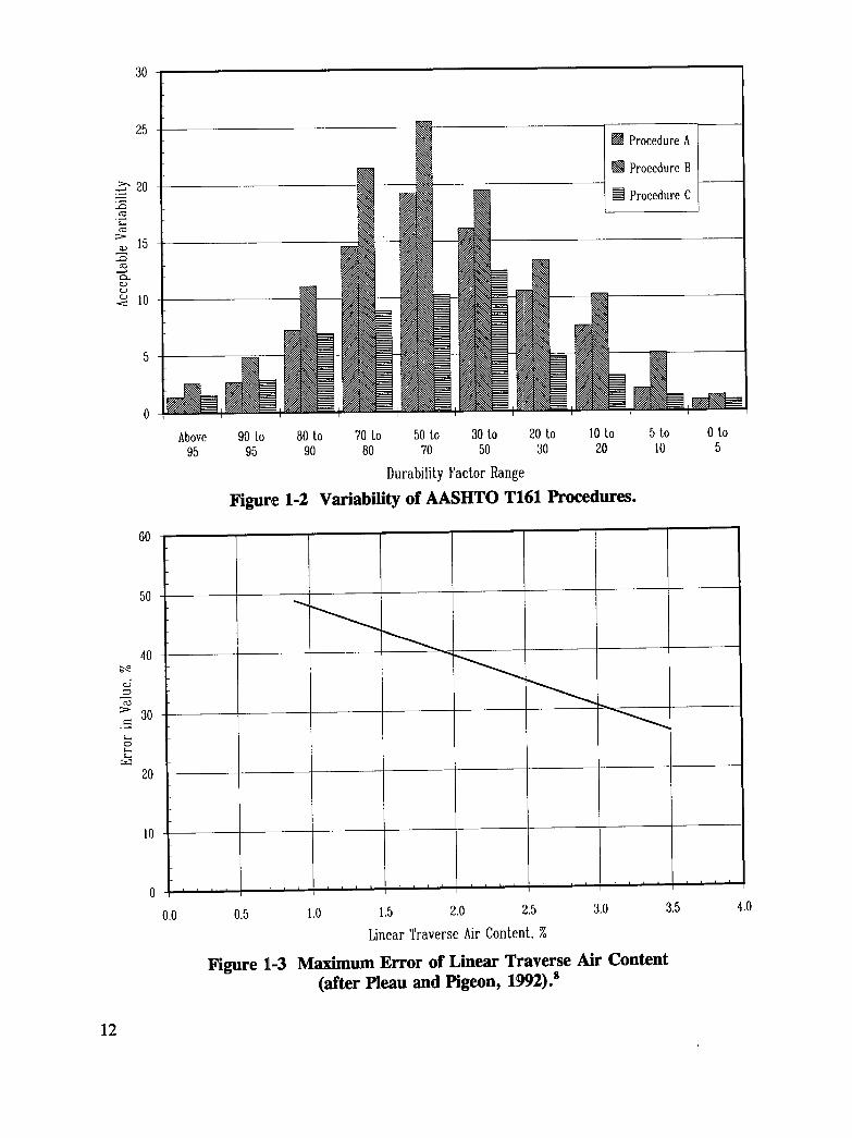
Section 3 of this report stated that the proposed Procedure C of AASHTO T 161 addressedperceived problems with the existing Procedures A and B. Procedure C also reduces thevariability in DF results in all but the highest and lowest DF ranges. Initial testing of cellsin Design Matrix A used nine or more specimens per cell to help estimate the number ofspecimens per cell that would be necessary to provide reasonable confidence in the results.Subsequent testing used a sample size of five specimens. The acceptable variability in theaverage DF determined for a group of five specimens is shown in figure 1-2. The variabilityshown is the "difference two-sigma limit (D2S)" as defined in ASTM Practice E 177 andcalculated as prescribed in ASTM Practice C 670. These values approximate the rangewithin which 95 percent of all means of five specimens from the same batch would fall.Variabilities are shown for Procedures A and B in addition to the proposed Procedure C.This figure clearly shows that Procedure C substantially reduces the variability, especially inthe intermediate DF ranges discussed in section 2.
5.2 Maximum Errors in Linear Traverse Results
When this investigation began, ASTM C 457 (1982 version) did not provide any informationon the precision of air-void parameters of hardened concrete determined by the lineartraverse method. The guidelines for minimum area of finished surface (71 cm 2) andminimum length of traverse (2.286 m) for a nominal maximum aggregate size of 19 mmwere observed. ASTM has since updated C 457 (1990 version) which includes someinformation on precision of linear traverse measurements. Pleau and Pigeon 8 publishedprocedures for calculating the expected precision of the various hardened air-voidparameters given information on traverse length, area, number of voids intercepted, etc. 8These latter procedures were used for the maximum error values shown. All are for the 95percent confidence range, described as (D2S) in ASTM Practice C 670.
10
Air Content of Hardened Concrete - The maximum expected error expressed as a percent ofthe air content value is shown in figure 1-3. This error is rather high, in part due to the lowair contents emphasized in this study, and in part due to the influence that large voids haveon the air content determination.
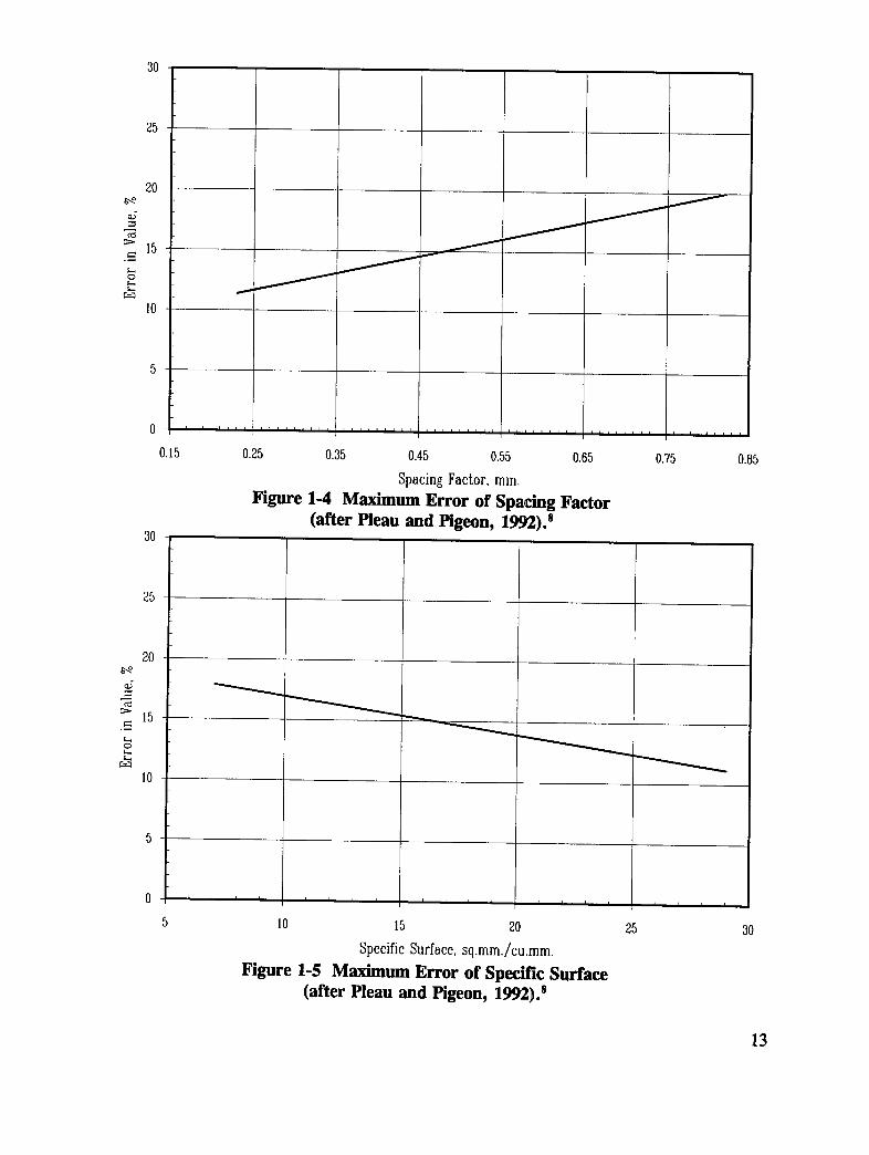
Spacing Factor - Figure 1-4 shows the maximum expected error in the L values presented inappendix E. The maximum error is expressed as a percentage of the measured value.
Specific Surface - The maximum expected error in a is shown in figure 1-5. This error isalso given as a percent of the measured value.
Philleo Factor - The maximum expected error in P was not calculated. Because this valuewas determined from a curve-fit of the air-void chord length data, the maximum expectederror should be substantially less than that shown for L.
Attiogbe's Mean Void Spacing4 - The maximum expected error in S was not calculated, butthe error is probably significantly greater than that shown for L. This is due to therespective methods of calculating L and S. L is proportional to p/A, where p is the volumefraction paste content and A is the volume fraction air content of the concrete, determined asdescribed in ASTM C 457. S, however, is proportional to p2/A. The error in p determinedby the linear traverse method for the mixes included in this study typically ranged from 15 to20 percent (as determined by the procedures set forth by Pleau and PigeonS). This additionalerror would be expected to increase the variability for S values.
The possible errors in the various air-void parameters determined by linear traverse analysisare greater than originally anticipated, and may perhaps be too large to permit acceptablemodelling of the requirements for frost-resistant concrete. Portions of specimens remainingafter rapid freezing and thawing for all of the batches tested have been retained by theresearch team, and slices of these specimen portions are being prepared for inclusion in theStrategic Highway Research Program (SHRP) Materials Reference Library. This referencelibrary is being maintained under supervision of the Federal Highway Administration(FHWA). Requests for access to these specimens should be directed to:
Federal Highway AdministrationHNR-20
6300 Georgetown PikeMcLean, VA 22101
11
3O
25
[] ProcedureA
[] ProcedureB>" 20
:_ [] ProcedureCc_
0
Above 90 Lo 80 to 70 Lo 50 Lo 30to 20 to 10to 5 to 0 to95 95 90 80 70 50 30 20 10 5
DurabilityFactorRange
Figure 1-2 Variability of AASHTO T161 Procedures.
60
5O
4o_J
c_
30.=_
2O
10
i i i t f T i t i } i { { i i T I i i i _ i i i I I i i i i { i
0.0 0.5 l.O 1.5 2.0 2.5 3.0 3.5 4.0
Linear Traverse Air Content. 70
Figure 1-3 Maximum Error of Linear Traverse Air Content(after Pleau and Pigeon, 1992). 8
12
30
25
20 /-
> 15 ...-_
10
0 i i i IIIITJ ,i i ,J_lll i i i rill II ...... ' ' ' ' ' ' '' ' ' ' ' ,, *,,,,, I Lit, .....
O.15 0.25 0.35 0.45 0.55 0.65 0.75 0.65
SpacingFactor,mm.Figure 1-4 Maximum Error of Spacing Factor
(after Plean and Hgeon, 1992). s30
25
20
lO
0 i i i r i t i i I I _ I r i I i I I I I
5 10 15 20 25 30
SpecificSurface,sq.mm./cu.mm.
Figure 1-5 Maximm Error of Specific Surface(after Heau and Pigeon, 1992))
13
5.3 Reliability of Freezable Moisture Results
The reliability of the freezable moisture results is not known. ASTM C 642, "SpecificGravity, Absorption, and Voids in Hardened Concrete," suggests that "... the sample shallconsist of several individual portions of concrete ... each portion shall not be less than ...approximately 800 g." No precision information is given. ASTM C 127, "Specific Gravityand Absorption of Coarse Aggregate," specifies a minimum sample size of 3 kg for anaggregate that has a nominal size of 19 mm. An acceptable range of two percent-absorptionresults (D2S, ASTM Practice C 670) is given as 0.25 for aggregates with absorptions of lessthan 2 percent. The sample size for the equilibrium moisture content determinations wasapproximately 3 kg total for each humidity. The freezable moisture calculation involvestaking the difference between two moisture contents, but these moisture contents are from alinear fit of multiple moisture content-humidity measurements. Freezable moisturedeterminations for multiple sets of samples from the same concrete mix have not been made.Typical standard deviations for freezable moisture measurements from separate mixes butsimilar mix designs were 0.06 or less. This would suggest a maximum expected differencebetween freezable moisture determinations of similar mixes to be about 0.17 (D2S, ASTMPractice C 670). This estimate is preliminary, and should probably decrease as additionalfreezable moisture results are obtained for error analysis.
6.0 Frost-Resistance Model
No frost-resistance modelling has been attempted at this time. As of the preparation of thisreport, sufficient freezable moisture data has not been collected to adequately characterize theamount of freezable moisture in a given type of concrete mix (i.e., for a given w/c orw/(c+p), or a mix containing a high-range water reducer, etc.). Testing is continuing, andthe additional data will be made public as it becomes available.
7.0 Summary and Recommendations for Part I
The effects of the air-void and water-pore systems on the resistance of concrete to repeatedcycles of freezing and thawing were examined. To facilitate this work, one new testprocedure, and a modification of an existing test procedure were developed. The purpose ofdeveloping these procedures was to improve the precision of rapid freezing and thawingtesting. These new test procedures were used in the development of a database of air-void,water-pore, and DF information for a variety of concretes made with a range ofair-entraining admixtures, normal and high-range water-reducing admixtures, pozzolan typesand contents, and other mix and curing parameters. The test proo_.dure_ and database aresummarized on the next page.
14
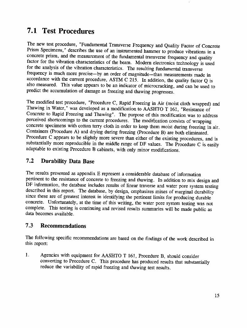
7.1 Test Procedures
The new test procedure, "Fundamental Transverse Frequency and Quality Factor of ConcretePrism Specimens," describes the use of an instrumented hammer to produce vibrations in aconcrete prism, and the measurement of the fundamental transverse frequency and qualityfactor for the vibration characteristics of the beam. Modem electronics technology is usedfor the analysis of the vibration characteristics. The resulting fundamental transversefrequency is much more precise--by an order of magnitude--than measurements made inaccordance with the current procedure, ASTM C 215. In addition, the quality factor Q isalso measured. This value appears to be an indicator of microcracking, and can be used topredict the accumulation of damage as freezing and thawing progresses.
The modified test procedure, "Procedure C, Rapid Freezing in Air (moist cloth wrapped) andThawing in Water," was developed as a modification to AASHTO T 161, "Resistance ofConcrete to Rapid Freezing and Thawing". The purpose of this modification was to addressperceived shortcomings to the current procedures. The modification consists of wrappingconcrete specimens with cotton terry cloth in order to keep them moist during freezing in air.Containers (Procedure A) and drying during freezing (Procedure B) are both eliminated.Procedure C appears to be slightly more severe than either of the existing procedures, and issubstantially more reproducible in the middle range of DF values. The Procedure C is easilyadaptable to existing Procedure B cabinets, with only minor modifications.
7.2 Durability Data Base
The results presented as appendix E represent a considerable database of informationpertinent to the resistance of concrete to freezing and thawing. In addition to mix design andDF information, the database includes results of linear traverse and water pore system testingdescribed in this report. The database, by design, emphasizes mixes of marginal durabilitysince these are of greatest interest in identifying the pertinent limits for producing durableconcrete. Unfortunately, at the time of this writing, the water pore system testing was notcomplete. This testing is continuing and revised results summaries will be made public asdata becomes available.
7°3 Recommendations
The following specific recommendations are based on the findings of the work described inthis report:
1. Agencies with equipment for AASHTO T 161, Procedure B, should considerconverting to Procedure C. This procedure has produced results that substantiallyreduce the variability of rapid freezing and thawing test results.
15
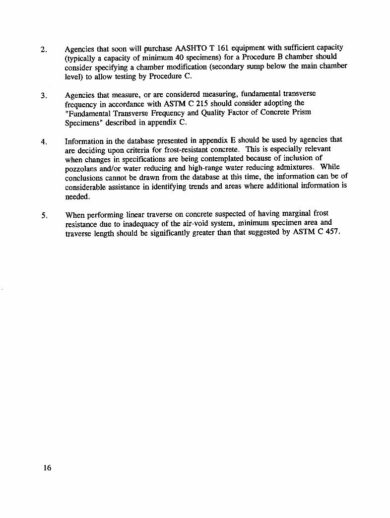
2. Agencies that soon will purchase AASHTO T 161 equipment with sufficient capacity(typically a capacity of minimum 40 specimens) for a Procedure B chamber shouldconsider specifying a chamber modification (secondary sump below the main chamberlevel) to allow testing by Procedure C.
3. Agencies that measure, or are considered measuring, fundamental transversefrequency in accordance with ASTM C 215 should consider adopting the"Fundamental Transverse Frequency and Quality Factor of Concrete PrismSpecimens" described in appendix C.
4. Information in the database presented in appendix E should be used by agencies thatare deciding upon criteria for frost-resistant concrete. This is especially relevantwhen changes in specifications are being contemplated because of inclusion ofpozzolans and/or water reducing and high-range water reducing admixtures. Whileconclusions cannot be drawn from the database at this time, the information can be ofconsiderable assistance in identifying trends and areas where additional information isneeded.
5. When performing linear traverse on concrete suspected of having marginal frostresistance due to inadequacy of the air-void system, minimum specimen area andtraverse length should be significantly greater than that suggested by ASTM C 457.
16
References
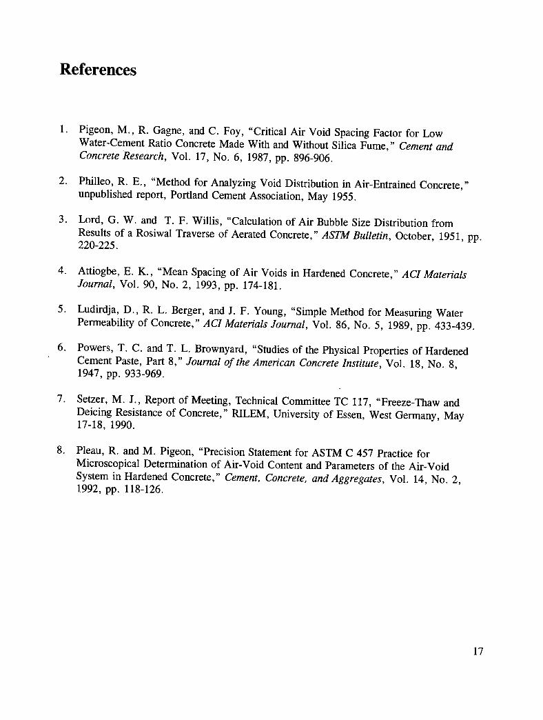
1. Pigeon, M., R. Gagne, and C. Foy, "Critical Air Void Spacing Factor for LowWater-Cement Ratio Concrete Made With and Without Silica Fume," Cement andConcrete Research, Vol. 17, No. 6, 1987, pp. 896-906.
2. Philleo, R. E., "Method for Analyzing Void Distribution in Air-Entrained Concrete,"unpublished report, Portland Cement Association, May 1955.
3. Lord, G. W. and T. F. Willis, "Calculation of Air Bubble Size Distribution fromResults of a Rosiwal Traverse of Aerated Concrete," ASTM Bulletin, October, 1951, pp.220-225.
4. Attiogbe, E. K., "Mean Spacing of Air Voids in Hardened Concrete," ACI MaterialsJournal, Vol. 90, No. 2, 1993, pp. 174-181.
5. Ludirdja, D., R. L. Berger, and J. F. Young, "Simple Method for Measuring WaterPermeability of Concrete," ACI Materials Journal, Vol. 86, No. 5, 1989, pp. 433-439.
6. Powers, T. C. and T. L. Brownyard, "Studies of the Physical Properties of HardenedCement Paste, Part 8," Journal of the American Concrete Institute, Vol. 18, No. 8,1947, pp. 933-969.
7. Setzer, M. J., Report of Meeting, Technical Committee TC 117, "Freeze-Thaw andDeicing Resistance of Concrete," RILEM, University of Essen, West Germany, May17-18, 1990.
8. Pleau, R. and M. Pigeon, "Precision Statement for ASTM C 457 Practice forMicroscopical Determination of Air-Void Content and Parameters of the Air-VoidSystem in Hardened Concrete," Cement, Concrete, and Aggregates, Vol. 14, No. 2,1992, pp. 118-126.
17
Appendix ADesign Matrices
Table A-1 Preliminary Tests for Statistical Calibration andNormal Concretes (Matrix A)
Water/Cement Ratio Air Content
Low Medium High
0.52 (A09) (A06) (A03)
0.45 (A08) (A05) (A02)
0/40 (A07) (A04) (A01)Cell numbers are shown in _arentheses.AEA1 used for all concrete mixtures.
Table A-2 Water Reducer and Air-Entraining Admixture Type (Matrix B)
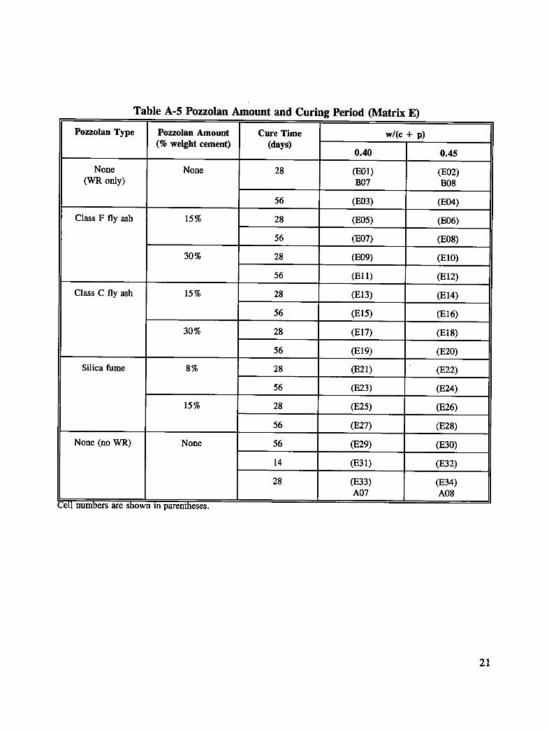
Table A-5 Pozzolan Amount and Curing Period (Matrix E)
Pozzolan Type Pozzolan Amount Cure Time w/(c + p)(% weight cement) (days)
0.40 0.45
None None 28 (E01) (E02)(WR only) B07 B08
56 (E03) (E04)
Class F fly ash 15% 28 (E05) (E06)
56 (E07) (E08)
30% 28 (E09) (El0)
56 (Ell) (E12)
Class C fly ash 15% 28 (E13) (E14)
56 (El5) (El6)
30% 28 (El7) (El8)
56 (El9) (E20)
Silica fume 8% 28 (E21) (E22)
56 (E23) (E24)
15% 28 (E25) (E26)
56 (E27) (E28)
None (no WR) None 56 (E29) (E30)
14 (E31) (E32)
28 (E33) (E34)A07 A08
2ell numbers are shown in parentheses.
21
Table A-6 List of Admixtures
AEA1 Daravair
AEA2 Microair
AEA3 Darex
WR Plastocrete 150
HRWR1 Elkem Proprietary (used in silica fumemixture below)
HRWR2 Sikament FF
P1 Class F fly ash, Centralia
P2 Class C fly ash, Laramie River
P3 Silica fume, Elkem Emsac F-100T
P4 Ground granulated blast furnace slag
22
Appendix BProposed Modifications to AASHTO T 161AASHTO Designation: TP17.
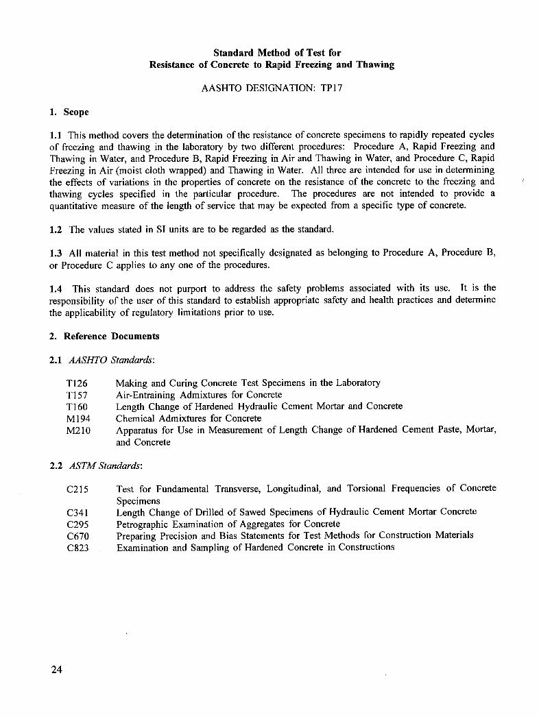
Standard Method of Test for
Resistance of Concrete to Rapid Freezing and Thawing
AASHTO DESIGNATION: TP17
1. Scope
1.1 This method covers the determination of the resistance of concrete specimens to rapidly repeated cyclesof freezing and thawing in the laboratory by two different procedures: Procedure A, Rapid Freezing andThawing in Water, and Procedure B, Rapid Freezing in Air and Thawing in Water, and Procedure C, RapidFreezing in Air (moist cloth wrapped) and Thawing in Water. All three are intended for use in determiningthe effects of variations in the properties of concrete on the resistance of the concrete to the freezing andthawing cycles specified in the particular procedure. The procedures are not intended to provide aquantitative measure of the length of service that may be expected from a specific type of concrete.
1.2 The values stated in SI units are to be regarded as the standard.
1.3 All material in this test method not specifically designated as belonging to Procedure A, Procedure B,or Procedure C applies to any one of the procedures.
1.4 This standard does not purport to address the safety problems associated with its use. It is theresponsibility of the user of this standard to establish appropriate safety and health practices and determinethe applicability of regulatory limitations prior to use.
2. Reference Documents
2.1 AASHTO Standards:
T126 Making and Curing Concrete Test Specimens in the LaboratoryT157 Air-Entraining Admixtures for ConcreteT160 Length Change of Hardened Hydraulic Cement Mortar and ConcreteM194 Chemical Admixtures for Concrete
M210 Apparatus for Use in Measurement of Length Change of Hardened Cement Paste, Mortar,and Concrete
2.2 ASTM Standards:
C215 Test for Fundamental Transverse, Longitudinal, and Torsional Frequencies of Concrete
SpecimensC34! Length Change of Drilled of Sawed Specimens of Hydraulic Cement Mortar ConcreteC295 Petrographic Examination of Aggregates for ConcreteC670 Preparing Precision and Bias Statements for Test Methods for Construction MaterialsC823 Examination and Sampling of Hardened Concrete in Constructions
24
3. Significance and Use
3.1 As noted in the scope, the two procedures described in this method are intended to determine the
effects of variations in both the properties and conditioning of concrete in the resistance to freezing andthawing cycles specified in the particular procedure. Specific applications include specified use inM194, T157, and ranking of coarse aggregates as to their effect on concrete freeze-thaw durability,especially where soundness of the aggregate is questionable.
3.2 It is assumed that the procedures will have no significantly damaging effects on frost-resistantconcrete which may be defined as (1) any concrete not critically saturated with water (that is, notsufficiently saturated to be damaged by freezing) and (2) concrete made with frost-resistant aggregatesand having an adequate air-void system that has achieved appropriate maturity and thus will preventcritical saturation by water under common conditions.
3.3 If, as a result of performance tests as described in this method, concrete is found to be relativelyunaffected, it can be assumed that it was either not critically saturated, or was made with "sound"aggregates, a proper air-void system, and allowed to mature properly.
3.4 No relationship has been established between the resistance to cycles of freezing and thawing ofspecimens cut from hardened concrete and specimens prepared in the laboratory.
4. Apparatus
4.1 Freezing and Thawing Apparatus:
4.1.1 The freezing and thawing apparatus shall consist of a suitable chamber or chambers in which thespecimens may be subjected to the specified freezing and thawing cycle, together with the necessaryrefrigerating and heating equipment and controls to produce continuously and automatically, reproduciblecycles within the specified temperature requirements. In the event that the equipment does not operateautomatically, provision shall be made for either its continuous manual operation on a 24-h a day basisor for the storage of all specimens in a frozen condition when the equipment is not in operation.
4.1.2 The apparatus shall be so arranged that, except for necessary supports, each specimen is (1) forProcedure A, completely surrounded by not less than 1 mm (1/32 in.) nor more than 3 mm (1/8 in.) ofwater at all times while it is being subjected to freezing and thawing cycles, or (2) for Procedure B or C,completely surrounded by air during the freezing phase. Specimens for Procedure C should be wrappedwith cotton terrycloth to keep the specimens wet during freezing. Rigid containers, which have thepotential to damage specimens, are not permitted. Length change specimens in vertical containers shallbe supported in a manner to avoid damage to the gage studs.
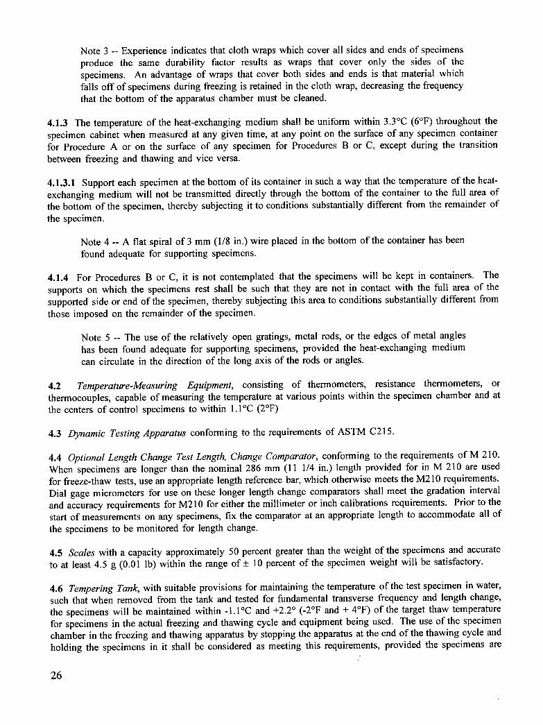
Note 1 -- Freezing and Thawing apparatus used for Procedure C, having above-groundsumps, may need modification to allow excess water drainage from the cloth wraps todrain out of the chamber. A miniature sump (approximately 20 to 40-L (5 to 10-gallon)capacity) added to the drain line between the chamber and the drain pump, below thelevel of the bottom of the chamber, should be sufficient.
Note 2 -- Experience has indicated that ice or water pressure, during freezing tests,particularly in equipment that uses air rather than a liquid as the heat transfer medium,can cause excessive damage to rigid metal containers, and possibly to the specimenstherein. Results of tests during which bulging or other distortion of containers occursshould be interpreted with caution.
25
Note 3 -- Experience indicates that cloth wraps which cover all sides and ends of specimensproduce the same durability factor results as wraps that cover only the sides of thespecimens. An advantage of wraps that cover both sides and ends is that material whichfalls off of specimens during freezing is retained in the cloth wrap, decreasing the frequencythat the bottom of the apparatus chamber must be cleaned.
4.1.3 The temperature of the heat-exchanging medium shall be uniform within 3.3°C (6°F) throughout thespecimen cabinet when measured at any given time, at any point on the surface of any specimen containerfor Procedure A or on the surface of any specimen for Procedures B or C, except during the transitionbetween freezing and thawing and vice versa.
4.1.3.1 Support each specimen at the bottom of its container in such a way that the temperature of the heat-exchanging medium will not be transmitted directly through the bottom of the container to the full area ofthe bottom of the specimen, thereby subjecting it to conditions substantially different from the remainder ofthe specimen.
Note 4 -- A flat spiral of 3 mm (1/8 in.) wire placed in the bottom of the container has beenfound adequate for supporting specimens.
4.1.4 For Procedures B or C, it is not contemplated that the specimens will be kept in containers. Thesupports on which the specimens rest shall be such that they are not in contact with the full area of thesupported side or end of the specimen, thereby subjecting this area to conditions substantially different fromthose imposed on the remainder of the specimen.
Note 5 -- The use of the relatively open gratings, metal rods, or the edges of metal angleshas been found adequate for supporting specimens, provided the heat-exchanging mediumcan circulate in the direction of the long axis of the rods or angles.
4.2 Temperature-Measuring Equipment, consisting of thermometers, resistance thermometers, orthermocouples, capable of measuring the temperature at various points within the specimen chamber and atthe centers of control specimens to within 1.1°C (2°F)
4.3 Dynamic Testing Apparatus conforming to the requirements of ASTM C215.
4.4 Optional Length Change Test Length, Change Comparator, conforming to the requirements of M 210.When specimens are longer than the nominal 286 mm (11 1/4 in.) length provided for in M 210 are usedfor freeze-thaw tests, use an appropriate length reference bar, which otherwise meets the M210 requirements.Dial gage micrometers for use on these longer length change comparators shall meet the gradation intervaland accuracy requirements for M210 for either the millimeter or inch calibrations requirements. Prior to thestart of measurements on any specimens, fix the comparator at an appropriate length to accommodate all of
the specimens to be monitored for length change.
4.5 Scales with a capacity approximately 50 percent greater than the weight of the specimens and accurateto at least 4.5 g (0.01 lb) within the range of + 10 percent of the specimen weight will be satisfactory.
4.6 Tempering Tank, with suitable provisions for maintaining the temperature of the test specimen in water,such that when removed from the tank and tested for fundamental transverse frequency and length change,
the specimens will be maintained within -1.1°C and +2.2 ° (-2°F and + 4°F) of the target thaw temperaturefor specimens in the actual freezing and thawing cycle and equipment being used. The use of the specimenchamber in the freezing and thawing apparatus by stopping the apparatus at the end of the thawing cycle and
holding the specimens in it shall be considered as meeting this requirements, provided the specimens are
26
the thawing cycle and holding the specimens in it shall be considered as meeting this requirements,provided the specimens are tested for fundamental transverse frequency within the above temperaturerange. It is required that the same target specimen thaw temperature be used throughout the testing of anindividual specimen since a change in specimen temperature at the time of length measurement canaffect the length of the specimen significantly.
5. Freezing and Thawing Cycle
5.1 Base conformity with the requirements for the freezing and thawing cycle on temperaturemeasurements of control specimens of similar concrete to the specimens under test in which suitabletemperature-measuring devices have been imbedded. Change the position of these control specimensfrequently in such a way as to indicate the extremes of temperature variation at different locations in thespecimen cabinet.
5.2 The nominal freezing and thawing cycle for both procedures of this method shall consist ofalternately lowering the temperature of the specimens from 4.4 to -17.8°C (40 to 0°F) and raising it from-17.8 to 4.4°C (0 to 40°F) in not less than 2 nor more than 4 h. for Procedure A, not less than 25 percentof the time shall be used for thawing, and for Procedures B or C, not less than 20 percent of the timeshall be used for thawing (Note 6). At the end of the cooling period the temperature at the centers of thespecimens shall be -17.8 + 1.7°C (0 + 3°F), and at the end of the heating period the temperature shall be4.4 + 1.7°C (40 + 3°F) with no specimen at any time reaching a temperature lower than -19.4°C (-3°F)nor higher than 6.1°C (43°F). The time required for the temperature at the center of any single specimento be reduced from 2.8 to -16.1°C (37 to 3°F) shall be no less than one-half of the length of the coolingperiod, and the time required for the temperature at the center of any single specimen to be raised from-16.1 to 2.8°C (3 to 37°F) shall not be less than one-half of the length of the heating period. For
specimens to be compared with each other, the time required to change the temperature at the centers ofany specimens from 1.7 to -12.2°C (35 to 10°F) shall not differ by more than one-third of the length ofthe heating period from the time required for any specimen.
Note 6 -- In most cases, uniform temperature and time conditions can be controlled mostconveniently by maintaining a capacity load of specimens in the equipment at all times.In the event that a capacity load of test specimens is not available, dummy specimens canbe used to fill empty spaces. This procedure also assists greatly in maintaining uniformfluid level conditions in the specimen and solution tanks. The testing of concretespecimens composed of widely varying materials or with widely varying thermalproperties, in the same equipment at the same time, may not permit adherence to thetime-temperature requirements for all specimens. It is advisable that such specimens betested at different times and that appropriate adjustments be made to the equipment.
5.3 The difference between the temperature at the center of a specimen and the temperature at itssurface shall at no time exceed 27.8°C (50°F).
5.4 The period of transition between the freezing and thawing phases of the cycle shall not exceed 10minutes, except when specimens are being tested in accordance with 8.2.
6. Sampling
6.1 Constituent materials for concrete specimens made in the laboratory shall be sampled usingapplicable standard methods.
6.2 Samples cut from hardened concrete are to be obtained in accordance with ASTM Practice C823.
27
7. Test Specimens
7.1 The specimens for use in this test shall be prisms made and cured in accordance with the applicablerequirements of T126 and M210.
7.2 Specimens used shall not be less than 76 mm (3 in.) nor more than 127 mm (5 in.) in width, depth,or diameter, and not less than 279 mm (11 in.) nor more than 406 mm (16 in.) in length.
7.3 Test specimens may also be cores or prisms cut from hardened concrete. If so, the specimensshould not be allowed to dry to a moisture condition below that of the structure from which taken. Thismay be accomplished by wrapping in plastic or by other suitable means. The specimens so obtainedshall be furnished with gage studs in accordance with ASTM C341.
7.4 For this test the specimens shall be sorted in saturated lime water from the time of their removalfrom the holds until the time freezing and thawing tests are started. All specimens to be compared witheach other initially shall be of the same nominal dimensions.
8. Procedure
8.1 Immediately after the specified curing period (Note 7), bring the specimen to a temperature within-3.1°C and +2.2°C (-2°F and +4°F) of the target that temperature that will be used in the freeze-thawcycle and test for fundamental transverse frequency, determine the mass, determine the average lengthand cross-section dimensions of the concrete specimen within the tolerance required in ASTM C215, anddetermine the initial length comparator reading (optional) for the specimen with the length changecomparator. Protect the specimens against loss of moisture between the time of removal from curing andthe start of the freezing and thawing cycles.
Note 7 -- Unless some other age is specified, the specimens should be removed fromcuring and freezing and thawing tests started when the specimens are 14 days old.
8.2 Start freezing and thawing tests by placing the specimens in the thawing water at the beginning ofthe thawing phase of the cycle. Remove the specimens from the apparatus, in a thawed condition, atintervals not exceeding 36 cycles of exposure to the freezing and thawing cycles, test for fundamentaltransverse frequency and measure length change (optional) with the specimens within the temperaturerange specified for the tempering tank in 4.6, determine the mass of each specimen, and return them tothe apparatus. To ensure that the specimens are completely thawed and at the specified temperature,place them in the tempering tank or hold them at the end of the thaw cycle in the freezing and thawingapparatus for a sufficient time for this condition to be attained throughout each specimen to be tested.Protect the specimens against loss of moisture while out of the apparatus and turn them end-for-endwhen returned. For Procedure A, rinse out the container and add clean water. Return the specimens
either to random positions in the apparatus or to positions according to some predetermined rotationscheme that will ensure that each specimen that continues under test for any length of time is subjectedto conditions in all parts of the freezing apparatus. Continue each specimen in the test until it has beensubjected to 300 cycles or until its relative dynamic modulus of elasticity reaches 60 percent of the initialmodulus, whichever occurs first, unless other limits are specified (Note 8). For the optional lengthchange test, 0.10 percent expansion may be used as the end of test. Whenever a specimen is removedbecause of failure, replace it for the remainder of the test by a dummy specimen. Each time a specimenis tested for fundamental frequency (Note 9) and length change, make a note of its visual appearance andmake special comment on any defects that develop. (Note 10) When it is anticipated that specimensmay deteriorate rapidly they should be tested for fundamental transverse frequency and length change(optional) at intervals not exceeding 10 cycles when initially subjected to freezing and thawing.
28
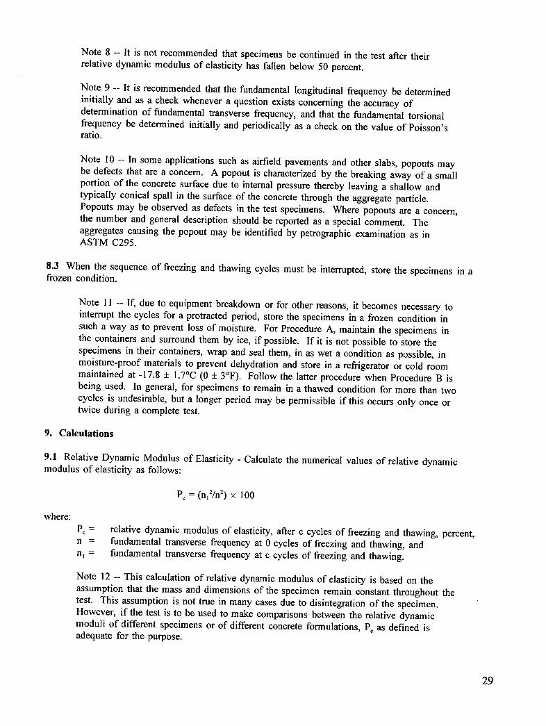
Note 8 -- It is not recommended that specimens be continued in the test after theirrelative dynamic modulus of elasticity has fallen below 50 percent.
Note 9 -- It is recommended that the fundamental longitudinal frequency be determinedinitially and as a check whenever a question exists concerning the accuracy ofdetermination of fundamental transverse frequency, and that the fundamental torsionalfrequency be determined initially and periodically as a check on the value of Poisson'sratio.
Note 10 -- In some applications such as airfield pavements and other slabs, popouts maybe defects that are a concern. A popout is characterized by the breaking away of a smallportion of the concrete surface due to internal pressure thereby leaving a shallow andtypically conical spall in the surface of the concrete through the aggregate particle.Popouts may be observed as defects in the test specimens. Where popouts are a concern,the number and general description should be reported as a special comment. Theaggregates causing the popout may be identified by petrographic examination as inASTM C295.
8.3 When the sequence of freezing and thawing cycles must be interrupted, store the specimens in afrozen condition.
Note 11 -- If, due to equipment breakdown or for other reasons, it becomes necessary tointerrupt the cycles for a protracted period, store the specimens in a frozen condition insuch a way as to prevent loss of moisture. For Procedure A, maintain the specimens inthe containers and surround them by ice, if possible. If it is not possible to store thespecimens in their containers, wrap and seal them, in as wet a condition as possible, inmoisture-proof materials to prevent dehydration and store in a refrigerator or cold roommaintained at -17.8 + 1.7°C (0 + 3°F). Follow the latter procedure when Procedure B isbeing used. In general, for specimens to remain in a thawed condition for more than twocycles is undesirable, but a longer period may be permissible if this occurs only once ortwice during a complete test.
9. Calculations
9.1 Relative Dynamic Modulus of Elasticity - Calculate the numerical values of relative dynamicmodulus of elasticity as follows:
Pc = (nl2/n2) x 100
where:
Pc = relative dynamic modulus of elasticity, after c cycles of freezing and thawing, percent,n = fundamental transverse frequency at 0 cycles of freezing and thawing, andn_ = fundamental transverse frequency at c cycles of freezing and thawing.
Note 12 -- This calculation of relative dynamic modulus of elasticity is based on theassumption that the mass and dimensions of the specimen remain constant throughout thetest. This assumption is not true in many cases due to disintegration of the specimen.However, if the test is to be used to make comparisons between the relative dynamicmoduli of different specimens or of different concrete formulations, Pc as defined isadequate for the purpose.
29
9.2 Durability Factor - Calculate the durability as follows:
DF = PN/Mwhere:
DF = durability factor of the test specimen,P = relative dynamic modulus or elasticity at N cycles, percent,
N = number of cycles at which P reaches the specified minimum value for discontinuing thetest or the specified number of cycles at which the exposure is to be terminated,whichever is less, and,
M = specified number of cycles at which the exposure is to be terminated.
9.3 Length Change in Percent (Optional) - Calculate the length change as follows:
(/2 - 11)Lc - -- × 100L
g
where:
Lc = length change of the test specimen after c cycles of freezing and thawing, percent,11= length comparator reading at 0 cycles,12= length comparator reading after c cycles, and
Lg = the effective gage length between the innermost ends of the gage studs as shown in themold diagram in M210.
10. Report
10.1 Report the following data such as are pertinent to the variable or combination of variables studiedin the test:
10.2 Properties of Concrete Mixture:
10.2.1 Type and proportions of cement, fine aggregate, and coarse aggregate, including maximum sizeand grading (or designated grading indices), and ratio of net water content to cement.
10.2.2 Kind and proportion of any addition or admixture used.
10.2.3 Air content of fresh concrete.
10.2.4 Unit weight of fresh concrete.
10.2.5 Consistency of fresh concrete.
10.2.6 Air content of the hardened concrete when available.
10.2.7 Indicate if the test specimens are cut from hardened concrete, and if so, state the size, shape,
orientation of the specimens in the structure, and an other pertinent information available.
10.2.8 Curing Period.
10.3 Mixing, Molding, and Curing Procedures - Report any departures from the standard procedures formixing, molding, and curing as prescribed in Section 7.
30
10.4 Procedure - Report which of the three procedures was used.
10.5 Characteristics of Test Specimens:
10.5.1 Dimensions of specimens at 0 cycles of freezing and thawing.
10.5.2 Mass of specimens at 0 cycles of freezing and thawing, and
10.5.3 Nominal gage length between embedded ends of gage studs, and
10.5.4 Any defects in each specimen present at 0 cycles of freezing and thawing.
10.6 Results:
10.6.1 Values for the durability factor of each specimen and for the average durability factor for eachgroup of similar specimens, and the specified values for minimum relative dynamic modulus andmaximum number of cycles (Note 13).
10.6.2 Values for he percent length change of each specimen and for the average percent length changefor each group of similar specimens (Note 13).
10.6.3 Values of loss or gain of mass for each specimen and average values for each group of similarspecimens, and
10.6.4 Any defects in each specimen which develop during testing, and the number of cycles at whichsuch defects were noted.
Note 13 -- It is recommended that the results of the test on each specimen, and the
average of the results on each group of similar specimens, be plotted as curves showingthe value of relative modulus of elasticity or percent length change against timeexpressed as the number of cycles of freezing and thawing.
11. Precision
11.1 Within-Laboratory Precision (Single Beams) - Criteria for judging the acceptability of durabilityfactor results obtained by the three procedures in the same laboratory on concrete specimens made fromthe same batch of concrete or from two batches made with the same materials are given in Table 1.Precision data for length change (optional) are not available at this time.
Note 14 -- The between-batch precision of durability factors has been found to be thesame as the within-batch precision. Thus, the limits given in this precision statementapply to specimens from different batches made with the same materials and mix designand having the same air content as well as to specimens from the same batch.
Note I5 -- The precision of this method for both procedures has been found to dependprimarily on the average durability factor and not on the maximum N or minimum Pspecified for terminating these test nor on the size of the beams within limits. The dataon which test precision statements are based cover maximum N's from 100 to 300 cycles,and minimum P's from 50 to 70 percent of Eo. The indexes of precision are thus valid atleast over these ranges.
31
11.1.1 The different specimen sizes represented by the data include the following: 76 by 76 by 406
mm; 76 by 76 by 416 mm; 76 by 102 by 406 mm; 89 by 114 by 406 mm; 76 by 76 by 279 mm; 89 by102 by 406 mm; and 102 by 76 by 406 mm. (3 by 3 by 16 in.; 3 x 3 by 16¼ in.; 3 by 4 by 16 in.; 315by 41/2by 16 in.; 3 by 3 by 11 in.; 3tA by 4 by 16 in.; and 4 by 3 by 16 in.) The first dimension givenrepresents the direction in which the specimens were vibrated in the test for fundamental transversefrequency. The most commonly used size was 76 by 102 by 406 mm (3 by 4 by 16 in.).
11.2 Within-Laboratory Precision (Averages of Two or More Beams) - Specifications sometimes call forcomparisons between averages of two or more beams. Tables 2, 3 and 4 give appropriate standarddeviations and acceptable ranges for the three procedures for two averages of the number of test beamsshown.
11.3 Multilaboratory Precisions - No data are available for evaluation of multilaboratory precision. It isbelieves that a multilaboratory statement of precision is not appropriate because of the limited possibilitythat two or more laboratories will be performing freezing and thawing tests on the same concrete.
12. Between Procedure Comparisons
12.1 Comparison of Two Procedures Run Concurrently in the Same Chamber - Limited data comparingresults of specimens from the same batch, tested in accordance with Procedures A and C concurrently inthe same freezing and thawing apparatus are shown in Table 5. Concurrent comparison of eitherProcedure A or Procedure C with Procedure B in the same freezing and thawing apparatus is not
possible because the temperature conditions given in Section 5 cannot be simultaneously met forProcedure B and either of the other two procedures.
TABLE 1 Within-Laboratory Durability Factor Precision for Single Beams
Range of Procedure A Procedure B Procedure CAverage
Durability Acceptable Acceptable Acceptable
Factor Standard Range of Standard Range of Standard Range ofDeviation ^ Two Results ^ Deviation ^ Two Results ^ Deviation ^ Two Results ^
0 to 5 0.8 2.2 1.1 3.0 0.7 2.0
5 to 10 1.5 4.4 4.0 11.4 1.0 2.8
10 to 20 5.9 16.7 8.1 22.9 2.2 6.2
20 to 30 8.4 23.6 10.5 29.8 3.4 9.6
30 to 50 12.7 35.9 15.4 43.5 8.8 24.9
50 to 70 15.3 43.2 20.1 56.9 7.3 20.7
70 to 80 11.6 32.7 17.1 48.3 6.3 12.8
80 to 90 5.7 16.0 8.8 24.9 4.9 13.9
90 to 95 2.1 6.0 3.9 11.0 2.1 5.9
Over 95 1.1 3.1 2.0 5.7 1.1 3.1
NOTE -- The values given in Columns 2, 4 and 6 are the standard deviations that have been found to be
appropriate for Procedures A, B and C, respectively, for tests for which the average durability factor as in the
corresponding range given in Column 1. The values given in Columns 3, 5 and 7 are the corresponding limitsthat should not be exceeded by the difference between the results of two single test beams.
^ These numbers represent the (IS) and (D2S) limits as described in ASTM C 670
32
TABLE 2 Within-Laboratory Durability Factor Precision for Averages of Two or More Beams--Procedure A
Range of Number ofBeams Averaged
Average 2 3 4 5 6Durability
Factor Standard Acceptable Standard [Acceptable _landard [Acceptable Standard [Acceptable _tandard [Acceptable
Deviation A Range A Deviation ^ [Range A Deviation ^ _,ange A Deviation ^ _,ange ^ Deviation n ]Range n
^These numbers represent the (1S) and (D2S) limits as described in ASTM C 670
34
Appendix CStandard Test Method for Determining the FundamentalTransverse Frequency and Quality Factor of Concrete PrismSpecimens
Standard Test Method for Determiningthe Fundamental Transverse Frequency andQuality Factor of Concrete Prism Specimens
AASHTO Designation TP181
1. Scope
1.1 This test method describes procedures for determining the fundamental transverse frequency andquality factor of concrete prism specimens for the purpose of non-destructively evaluating thecondition of the concrete.
1.2 The values stated in SI units are to be regarded as the standard. The values in parentheses arefor informational purposes only.
1.3 This procedure may involve hazardous materials, operations, and equipment. Thisprocedure does notpurport to address all of the safety problems associated with its use. It is the responsibility of whoever uses thisprocedure to consult and establish appropriate safety and health practices and determine the applicability ofregulatory limitations prior to use.
2. Referenced Documents
2.1 AASHTO Standards
R9 Acceptance Sampling Plans for Highway Construction"1"23Making and Curing Concrete Test Specimens in the FieldT24 Test Method for Obtaining and Testing Drilled Cores and Sawed Beam_of Concrete
T126 Making and Curing Concrete Test Specimens in the LaboratoryT161 Test Method for Resistance of Concrete to Rapid Freezing and Thawing
2.2 ASTM Standards
C215 Standard Test Method for Fundamental Transverse, Longitudinal, and Torsional Frequencies ofConcrete Specimens
C670 Practice for Preparing Precision and Bias Statements for Test Methods for Construction MaterialsD3665 Random Sampling of Construction MaterialsEl05 Probability Sampling of MaterialsE122 Choice of Sample Size to Estimate the Average Quality of a Lot or ProcessEl41 Acceptance of Evidence Based on the Results of Probability Sampling
3. Terminology
3.1 Description of Terms Specific to this Standard
IThis standard is based on SHRP Product 2019.
36
3.1.1 Quality Factor (Q) - the normalized width of the frequency response curve - the inverse of the measureof internal damping
3.1.2 Fundamental Transverse Frequency - the frequency at which a specimen vibrates in the transverse modewith the greatest amplitude for a given amount of input excitation. This frequency is sometimes termed thefrequency at which a specimen resonates.
4. Summary of Method
4.1 The fundamental transverse frequency and the quality factor of a concrete prism are determined byanalyzing the vibration frequency response spectrum produced when the prism is lightly struck.
4.2 The specimen is supported in such a way as to minimize interference with vibration of the specimen.
4.3 The measured time response of the beam vibrations is converted into a frequency response by a FastFourier Transform (FFT). The fundamental transverse frequency and quality factor are then determined byfitting a standard frequency response curve to the measured frequency data.
5. Significance and Use
5.1 This test method is intended primarily for determining the amount of deterioration produced by accelerateddurability tests such as T161. The deterioration can be quantified either by evaluating changes in the dynamicmodulus of elasticity, or by evaluating changes in the quality factor of the concrete.
5.2 Deterioration from accelerated durability tests results in a decrease in elastic modulus of concretespecimens. This decrease is measured as a decrease in fundamental transverse frequency.
5.3 Prior to the accumulation of sufficient deterioration to produce a measurable decrease in fundamentaltransverse frequency, a decrease in quality factor occurs. This decrease in quality factor is thought to be anindication of micro-cracking in the concrete specimen. Though the microcracking may not be of sufficientmagnitude to produce a change in the fundamental transverse frequency, it does change the amount of internaldamping of the vibrations in the specimen.
6. Interferences
6.1 Improper tensioning of the wires supporting the specimen during testing will affect the test results.
6.2 Insecure attachment of the accelerometer to the test specimen surface will affect the test results.
6.3 Improper positioning of the impact point on the test specimen surface will affect the test results.
6.4 Failure to completely damp test specimen vibrations before application of each test impact will affect thetest results.
6.5 Supporting the test specimen at locations other than the nodal points of the specimen will affect the testresults.
6.6 Using test specimens with shapes and/or dimensions other than those indicated will affect the test results.
37
7. Apparatus
7.1 Fourier Analyzer - The Fourier analyzer used shall meet the following requirements when coupled withthe data analysis and control component:
7.1.1 The Fourier analyzer shall be capable of FFT analysis of vibrational input data to convert time-domainmeasurements to frequency-domain response.
7.1.2 The Fourier analyzer shall be capable of averaging multiple frequency response measurements from asingle specimen prior to determination of fundamental frequency and quality factor.
7.1.3 The Fourier analyzer shall be equipped with a minimum of two input channels.
7.1.4 The Fourier analyzer shall be capable of using the signal from one channel to normalize the signal from asecond channel, thus allowing multiple readings to be averaged even though the vibration responses may havebeen produced by different impact magnitudes.
7.1.5 The Fourier analyzer shall be capable of using a minimal input level in one channel to trigger recordingof data in all channels.
7. 1.6 The Fourier analyzer shall be equipped with controls for lower and upper limits of the frequency rangethat may be set independently.
Note 1 -- The lower limit of the frequency range is set above the frequency of the rigid bodymotion of the specimen on the support. For the support described under Section 7.1.4 and a
normal-weight concrete specimen of dimensions 102 by 76 by 406 mm (4 by 3 by 16 in), alower limit of 100 Hz. is appropriate. The upper limit of the frequency range should be set _>500 Hz above the expected fundamental transverse frequency of the specimens to be measured.This upper limit should not be made too high as the precision of many Fourier analyzers isdependent upon the frequency range being analyzed. An upper limit of 3000 Hz is appropriatefor a normal-weight concrete specimen of dimensions 102 by 76 by 406 mm (4 by 3 by 16 in).
7.1.7 The Fourier analyzer shall be capable of recording the time history of the vibrations with an exponentialweighting or _window_.
Note 2 -- An exponential weighting of 0.1 provides the best reproducibility for both damagedand un-damaged concrete prisms. (The time response of a vibrating prism is the summation ofdecaying sinusoids. Included in the measurement is an essentially constant amount of noise.Thus, the signal-to-noise ratio decreases with measurement time. By treating the time-domainmeasurement to a decreasing exponential weighting, the readings with the best signal-to-noiseratio are weighted greater in the FFT analysis.) This procedure assists in obtaining the
reproducibility of the quality factor results given in Section 12.1.1.
7.1.8 The Fourier analyzer shall be capable of storing at least 1024 points for FFT analysis with a maximumfrequency capability > 8 kHz.
Note 3 -- A sampling size of 1024 points was found to give the most reproducible fundamentalfrequency and quality factor results on both damaged and undamaged prisms. Whileincreasing the sampling size from 512 to 1024 points decreased the variability, a highersampling size (2048 rather than 1024 points) increased variability. This is probably due to thelonger measurement time required for the larger number of points and the decreasing signal-to-noise
38
ratio with increasing sampling times.
7.1.9 The Fourier analyzer shall be capable of restricting the voltage range of any of the inputs that are usedfor analysis.
7.1.10 The Fourier analyzer shall be equipped with audible and/or visual feedback mechanisms to the operatorindicating when an impact of proper magnitude has been delivered.
Note 4 -- A sensitivity of 0.1 to 1.0 AC volts for the excitation channel and 0 to 5.0 AC voltsfor the vibration response channel are appropriate for the hammer and accelerometer describedin Sections 7.2 and 7.3, below.
7.1.11 The Fourier analyzer shall be capable of producing a visual display of the frequency response spectrumthrough the data recording and analysis component described in section 7.5.
7.2 Impact Hammer - A modally tuned impact hammer component capable of producing vibrations in the testspecimen by impact and meeting the following requirements:
7.2.1 The impact hammer shall be capable of producing a flat frequency response over the entire frequencyrange being sampled. A modally tuned impact hammer with a mass of 140 g and a frequency response of 0 to8 kHz produces the appropriate impact.
7.2.2 The impact hammer shall be equipped with a hammer impact tip of sufficient hardness and appropriateshape to neither be damaged by the specimen nor cause damage to the specimen when an impact of propermagnitude is produced. A spherical tip is not mandatory.
7.2.3 The impact hammer shall be equipped with an electronic load cell and appropriate power supply capableof producing an output voltage proportional to the magnitude of the impact with the specimen. The sensitivityof the load cell shall be 12.5 5:2.5 mV/N or better.
7.3 Accelerometer and Power Supply - The accelerometer shall have a flat base, a mass ___3 g, an operatingfrequency range of at least 10 to 10000 Hz, and a fundamental frequency at least twice the highest expectedfundamental frequency of any of the specimens to be measured. The accelerometer power supply shall providean output through the accelerometer-power supply combination of at least 50 mV/g.
Note 5 -- Amplification of the accelerometer output may be necessary to achieve the properoutput level.
7.4 Specimen Support - The specimen support shall be fabricated from 2 parallel 0.62 mm diameter pianowires that permit the specimen to vibrate freely, and minimize the amount of vibration energy absorbed fromthe specimen.
7.4.1 The parallel support wires shall be arranged to support the specimen a distance of 22.4 percent of thespecimen length from each end of the specimen. This is approxim:tely the location of the nodal points of thespecimen, and vibration magnitude will be minimal at these points.
7.4.2 The parallel support wires shall be positioned at least 25 mm above any horizontal table surface tofacilitate placing the specimens on the wires.
7.4.3 The length of the specimen support wires shall be at least 3 times the width of the specimen when thespecimen is placed on the support wires.
39
7.4.4 The parallel support wires shall be tensioned so that they vibrate when plucked at a frequency of at least400 Hz when there is no specimen on them thus minimizing system damping of the vibrations.
Note 6 -- Piano wires, 0.62 mm diameter and spanning a distance of 350 mm, have been
found to provide a suitable support for normal weight concrete prisms having dimensions of
102 by 762 by 406 mm (4 by 3 by 16 in).
7.5 Data Analysis and Control Equipment - The data analysis and control equipment shall include a personal
computer capable of controlling the equipment and recording the data as indicated in Section 7.1.1; performingdata analysis to determine fundamental transverse frequency and quality factor; and meeting the minimumcompatibility requirements specified by the manufacturer of the Fourier analysis equipment. The computer mayor may not be an integral part of the Fourier analysis equipment
7.5.1 The data analysis and control equipment shall include software adequate to perform the requiredfunctions. Software to accomplish the curve fit required in Section 11.1.3 is generally available from the
supplier of the Fourier analysis equipment or can be written by a person with programming experience andsome familiarity with modal analysis techniques.
Note 7 -- The curve fit is accomplished as a weighted circle fit in the complex Nyquist plane.
An appropriate weighting is the square of the distance from the origin in the Nyquist plane.Suggested references for additional information on modal analysis include: Modal Testing andPractice by D.J. Edwins, June, 1985; and assorted papers from the Seminar on UnderstandingDigital Control and Analysis in Vibration Test Systems, The Shock and Vibration InformationCenter, 1975.
8. Sampling and Test Specimens
8.1 Determine the number of samples needed based on the concrete under investigation and the purpose forwhich the test data will be used.
8.2 Samples obtained from concrete pavements and structures.
8.2.1 Stratified patterns for sampling are satisfactory for many concrete elements. On support or substructureelements, a significant factor in the location of sample sites is the geometry of the dement. In these casessmaller or larger stratified patterns or non-stratified patterns may be appropriate.
8.2.2 If a stratified pattern is used, locate the sample sites using a stratified random sampling procedure. Ifgeometry dictates a non-stratified pattern, use a random sampling procedure.
Note 8 -- If geometry of the concrete dement under investigation restricts available samplesites to 5 or less, it is generally desirable to sample from all available sites when practical.
Note 9 -- ASTM D3665 contains a table of random numbers, including instructions for use.Practices R9 and ASTM El05, E122, and El41 contain additional information concerning
sampling practices.
8.2.3 Obtain prismatic test specimens cut from hardened concrete in accordance with T24.
8.3 Sampling from Freshly Mixed Concrete in the Field.
40
8.3.1 Use a stratified random sampling plan for selection of samples from a concrete lot or production process.If the lot or production process is not suitable for stratification (i.e. limited quantity, intermittent batching ofsmall quantities of different concrete mixes, etc.) use a random sampling procedure.
8.3.2 Prepare prismatic test specimens in the field in accordance with T23.
8.4 Sampling from Freshly Mixed Concrete in the Laboratory.
8.4.1 Obtain constituent materials for concrete specimens made in the laboratory using applicable standardmethods.
8.4.2 Prepare prismatic test specimens in the laboratory in accordance with T126 or other appropriateprocedures.
8.5 Use specimens of rectangular cross section and appropriate dimensions so that fundamental frequencies ofeither of the two transverse modes, the torsional mode, and the longitudinal mode do not interfere with eachother. Square and round cross-sections specifically do not meet these requirements.
Note 10 -- The data analysis described in Section 11 includes as an assumption that thevibrations are from a single degree of freedom system. This means that other vibration modesare not contributing to the frequency response in the range of frequencies being analyzed. Aspecimen size of 102 by 76 by 406 mm (4 by 3 by 16 in) meets these requirements.
9. Standardization
9.1 Verify the calibration of the Fourier analyzer at least every 12 months. Use a reference beam with knownresponse for periodic quality control checks when testing is scheduled.
9.2 Verify calibration of the impact hammer and load cell at least every 12 months.
9.3 Verify calibration of the accelerometer at least evey 12 months.
10. Procedure
10.1 Place the specimen (Note 11) on the support wires so that the ends of the specimen extend equal amountsbeyond their respective support wires and the specimen is centered on the length of the wire. (Note 12)
Note 11 -- While the specimen can be tested across either cross-sectional axis, placing thespecimen so that cast or cut surfaces are on the top and bottom provide for easier and morereliable testing.
Note 12 -- Guide marks on the horizontal surface below the wires assist in rapidly placing theconcrete specimens in the correct alignment.
10.2 Attach the accelerometer to the specimen with a rubber band. Center the accelerometer on the top face ofthe specimen, as close to one end as possible. Arrange the base of the accelerometer securely on the specimen,and use a rubber band(s) with sufficient tension to keep the accelerometer firmly in contact with the specimen.
Note 13 -- While adhesive wax is the generally accepted method of temporarily attaching
41
accelerometersfor modal analysis, this method does not work well with specimens in the cooland dampcondition specified in Test Method T161. Drying any portion of the specimen topermituse of adhesive wax is not advised as this could produce variablequality factormeasurements. Adhesive wax or anothercoupling mediumcan be used in addition to a rubberband in an attemptto improve the contactbetweenthe accelerometerand the specimen, butthis has not been found to be necessary. If a couplingmedium is used, care shouldbe takentoprevent small amounts of scaled materialfrom becoming imbedded in the coupling mediumand preventinguniformcontactbetween the accelerometerand specimen.
10.3 Perform any necessary preparationsto the Fourieranalyzer and take a preliminaryreading of thefundamentaltransverse frequency by impactingthe top face of the specimen. Apply the impact vertically,centered on the top face, and on the end oppositeto the end on which the accelerometeris attached. Impactasnear as practicalto the end of the specimen. Record the hammer and accelerometerresponses, with saidrecording activatedby the hammerload cell response. The full frequencyresponse curvedisplayed may includemultiple response peaks, representingthe various transverseand torsionalvibrationalmodes. If the specimen isof appropriatedimensions, described in Section 8.5, and the accelerometerand impactare properlyplaced, asdescribed in sections 10.1 and 10.2 above, the greatestamplitude shown corresponds to the fundamentaltransverse frequency.
10.4 Using the approximatefundamentalfrequency from this initial impact, reset the frequency measurementrange to a total frequencyrange of 400 Hz, centeredon the approximatefundamentaltransversefrequency.
10.5 Make three successive impacts of the beam as described in Section 10.3, above, takingcare to stop anyvibrationsand/or rigid body swaying betweenimpacts. Observe the displayed frequencyresponsecurve aftereach impact, and repeat any that are not in the expected smooth shape. (Note 14) When the threeacceptablefrequencyresponses have been obtained, averagethe three responses and store this information for lateranalysis.
Note 14 - Specimen deteriorationwill cause the frequencyresponsecurve to become lesssmooth; this is normal behavior due to internal cracking in the specimen associatedwith thedeterioration.Major irregularities in the frequency response curve can generally be attributedto failing to completely stop movementof the specimen prior to makingthe impact. This canresult in vibrational interferencewhich looks like ajagged curve. In some cases, irregularitiesin the curve can also indicate that the accelerometer is not firmly seated on the specimen.
11. Interpretation and Calculation
11.1 Interpretation.
11.1.1 The fundamental transverse frequency, oJr, is the frequencywhich produces the highest amplitude in theaverage of the frequency response spectrums measured in Section 10.5, above.
11.1.2 The quality factor, Q, is the normalized width of the frequency response curve, and is defined as:
_0 r
Q -.
w2-°_l
42
where:
cor = the fundamental transverse frequency,
o_ = the frequency below oJ_at which the amplitude of the frequency response curve is [(2)°5]/2times that at wr, and
oJ2 = the frequency above o_r at which the amplitude of the frequency response curve is [(2)°s]/2times that at cor.
11.1.3 Actual calculation Of the fundamental transverse frequency and quality factor values is accomplished bythe computer software which fits a standard frequency response curve for a single degree of freedom system tothe measured data from Section 10.5, above.
11.2 Calculations
11.2.1 Calculate the dynamic Young's modulus of elasticity, E, in Pa, from the fundamental transversefrequency, mass, and dimensions of the test specimen as follows:
Dynamic E = Cm¢_o_2
where:
_o = the mass of the specimen, kg,oJr = the fundamental transverse frequency, Hz,Cm -- 0.9464(L3T/bt3), [(N)(sE)]/[(kg)(m2)],L = the length of the specimen, m,
t, b = the cross-section dimensions of the specimen, m, t being in the direction of vibration, and
T = a correction factor which depends on the ratio of radius of gyration, K, (K=0.2887 t) to thelength of the specimen, L, and on Poisson's ratio. Values of T for a Poisson's ratio of 1/6 aregiven in table 1.
11.2.1.1 Values of T for a Poisson's ratio of 1/6 are derived from Figure 1 of the paper by G. Pickett,"Equations for Computing Elastic Constants from Flexural and Torsional Resonant Frequencies of Vibration ofprisms and Cylinders", Proceedings, ASTM, Volume 45, 1945, P. 846. Poisson's ratio for water-saturated
concrete may be higher than 1/6. The correction factor, T', for a different value of Poisson's ratio, #m, and a
43
given K/L, may be calculated from the following relationship:
T' = T[1 +(0.26#+3.22#2)K/L]/[1 +0.1328(K/L)]
where:
T is taken from table 1 for the given K/L.
12. Report
12.1 Report the transverse frequency to the nearest Hz.
12.2 Report the quality factor.
13. Precision and Bias
13.1 Precision
13.1.1 The single operator, single laboratory precision for measurements of fundamental transverse frequencyand quality factor of a single specimen are shown in table 2. Values are shown for both an undamaged
specimen and a specimen whose relative dynamic modulus as defined in T161 has been reduced by repeatedcycles of freezing and thawing to approximately 60 percent. These results were determined for specimenshaving dimensions of 102 by 76 by 406 mm [4 by 3 by 16 in] (the first dimension is the direction of vibration).
TABLE 2 - Single Operator, Single Laboratory, Single Specimen Precision.
Fundamental Transverse Frequency Quality FactorSpecimenCondition Acceptable Range Acceptable Range
Coefficient of of 2 Results, Coefficient of of 2 Results,
Variation, percent ^ percent of mean ^ Variation, percent ^ percent of meanA
Un-Damaged 0.04 0.11 3.3 9.4
Specimen
Damaged 0.18 0.51 8.8 24.8Specimen
^ These numbers represent, respectively, the 1S% and the D2S% limits as described in theASTM Practice C 670.
a Specimen was reduced by the repeated cycles of freezing and thawing to approximately 60percent relative dynamic modulus as defined in Test Method T 161
13.1.2 Research required to determine the within-batch and between-batch precision of this method has notbeen conducted.
13.1.3 Research required to determine the among-laboratories precision of this method has not been conducted.
13.2 Bias - The research required to establish the bias of this method has not been conducted.
14. Keywords - concrete, Young's modulus of elasticity, fundamental transverse frequency, quality factor.
44
Appendix DDamping Measurements for Nondestructive Evaluation ofConcrete Beams
Synopsis
Change in relative dynamic modulus (RDM), as determined by resonance frequencymeasurements, is the most frequently used indicator for evaluating damage to concrete beamsthat are subjected to repeated cycles of freezing and thawing (ASTM C 666). Whilesinusoidal excitation (ASTM C 215) is the standard method for measuring resonancefrequency, impulse excitation has been approved by ASTM as an alternate. Importantadvantages of the impulse method are that it is rapid, quite reproducible, and also producesinformation on the damping characteristics of the vibrational modes with no additional
testing. The work reported in this paper identifies linear changes in damping with earlycycles of freezing and thawing before significant decreases in resonance frequency can beidentified. Comparisons of predicted and actual durability factors showed agreement withinpublished testing errors for most of the mixes tested. This work indicates that the durabilityfactor (ASTM C 666) can be accurately predicted with damping measurements before theactual failure of the concrete beams can occur from repeated cycles of freezing and thawing.
Introduction
The frost resistance of concrete is most frequently determined by subjecting concrete beamsto repeated cycles of freezing and thawing and periodically measuring the damage in thebeams. Because the measurement of damage must be nondestructive, measurement of theconcrete's vibration characteristics (modal analysis) has often been employed for damageevaluation. In 1938, Powers I presented a method comparing the musical tone of prisms aftera hammer impact with a calibrated set of orchestra bells to determine the specimen's dynamicmodulus of elasticity (proportional to resonance frequency). In his closure to writtendiscussion of his paper, Powers suggests that monitoring the change in the dynamic modulusof elasticity may indicate deterioration of a sample subjected to repeated cycles of freezingand thawing. The following year, Hornibrook 2 reported the use of electronics to moreaccurately match frequencies. This report was followed by the discovery of the use ofacoustic transducers to excite the specimens and scan for the frequency with maximumamplitude. Notable early research included Thomson in 19403, Obert and Duvall in 19414,Long and Kurtz in 19435, and Stanton in 1944. 6 In the following 20 years, manyinvestigations were performed to determine the results of this dynamic vibration on cement-based materials. 7-1° The method most commonly used today to evaluate damage in concretebeams subjected to repeated cycles of freezing and thawing, (ASTM C 666), still involvesthe determination of the resonance frequency of the beam (ASTM C 215). Present work
45
with damping measurements indicates that the durability factor can be accurately predictedbefore concrete beams fail due to repeated cycles of freezing and thawing. This takessubstantially less time than current procedures.
Background
Modal Analysis
Modal analysis has generally been used for nondestructive evaluation of the dynamiccharacteristics of a structure's modes of vibration. A mode of vibration is defined as the
deformation pattern of a structure at a natural frequency. Each mode of vibration isidentified by three factors: the resonance frequency; the damping factor; and the mode shape.Resonance frequency is the characteristic frequency at which a maximum response occurs fora given mode of vibration. The damping factor is a measure of the energy dissipated in eachcycle of vibration. A mode shape describes the deformed shape of a sample when subjectedto a dynamic system.
One method of modal testing uses sinusoidal excitation for the input signal. This methodforces a structure to vibrate at a frequency while the response of the structure is monitoredwith an accelerometer. The excitation frequency is varied until a maximum amplitude isobserved, which gives the resonance frequency for a particular mode of vibration. The
• sinusoidal excitation method is the current standard method for examining damage inconcrete prisms (ASTM C 215). 11
An alternative method of modal testing has recently been suggested as a possible way ofdetermining the resonance frequencies of concrete beams by investigators such as Malhotraand Carino 1_and Gaidis and Rosenberg. _2 The method uses impulse excitation. Forinstance, a hammer strike can be used to excite vibrations in a beam. A load cell on thehammer measures the impact force (input signal). The response of the beam is recorded withan accelerometer (output signal). A Fast Fourier Transform (FFT) transforms the timedomain data (amplitude as a function of time) into the frequency domain (amplitude as afunction of frequency). The ratio of the Fourier transform of the output signal to the Fouriertransform of the input signal is called the frequency response function. This function is acomplete mathematical description of the linear vibration characteristics of the prism over therange of frequencies determined by the hardware and software used.
Resonance Frequency, Relative Dynamic Modulus, and Durability Factor
As mentioned above, a mode of vibration is identified by a resonance frequency and adamping factor. A beam can vibrate at a number of frequencies at the same time. Theprimary, or resonance frequency, however, is the lowest frequency that has an amplitudesubstantially greater than both higher and lower frequencies. Figure D-1 shows a portion of
46
an idealized frequency response curve with the resonance frequency labelled. Isolating aportion of the frequency response curve like this essentially treats the vibration response as asingle degree of freedom system (SDOF). While vibrations outside of the limited rangearound the resonance frequency contribute to the overall response of the beam, they are oftenignored in modal analysis.
The dynamic modulus of elasticity for a concrete beam can be calculated from the resonancefrequency by the equation given in ASTM C 215:
ED= C "m • co_ (1)
where ED = dynamic modulus of elasticityC = shape, dimensions, and Poisson's ratio of the beamm = mass of the beam
t,or = resonance frequency of the beam
C is defined as follows for a prismatic beam:
0.00245 • L3T
C = bt3 (2)
where L = length of prismT = correction factor based on the ratio of the radius of gyration to the
length of the specimen, and on Poisson's ratioA sample with Poisson's ratio of 1/6, 16 in. (406 mm) long, and drivenin the 3-in. (76 mm) direction has a T factor of 1.24
b = dimensions of prismt = driving direction
Both C and codepend upon whether mode of vibration tested is longitudinal or transverse.Most tests of concrete beams subjected to freezing and thawing use transverse vibration.
As a concrete beam deteriorates from repeated cycles of freezing and thawing, EDand,therefore, cordecrease (ignoring mass and dimensional effects). The relative dynamicmodulus is a measure of this deterioration and is defined by ASTM C 666 as follows:
Pn = (cor* / cor02) " 100 (3)
where Pn = relative dynamic modulus after n cycles of freezing and thawing,coro = resonance frequency after n cycles of freezing and thawing, andcor* = resonance frequency at 0 cycles of freezing and thawing.
47
The effects of mass and dimension changes are ignored in the above equation but should beconsidered if there is significant change in mass.
A durability factor can be calculated for a concrete beam at the end of freezing and thawingtesting as follows (ASTM C 666):
DF = Pn " N/M (4)
where DF = durability factorN = number of cycles at which the testing is terminated (because either a
minimum Pn is reached or the specified number of cycles is reached)M = specified number of cycles
A typical value for M is 300 cycles and a typical minimum value for Pn is 60 percent (ASTMC 666). ASTM C 666 also allows the termination of the freezing and thawing testing if thespecimen exceeds a 0.10 percent length expansion.
Damping and Quality Factor
Malhotra and Carino 11have reviewed the damping properties of concrete. Research in
materials science by Coppola and Bradt 13 has suggested that viscous damping is moresensitive to thermal damage than elastic modulus. For analysis purposes, a quality factor (Q)is frequently used instead of viscous damping. While viscous damping increases withdeterioration, the quality factor decreases and is easier to monitor quantitatively. Q is relatedto viscous damping by the following equation:
Q = oJr/(2"o) (5)
where Q = quality factoro_r= resonance frequencytr = damping coefficient
Q is normally calculated as follows:
Q = wl I(wz-Wl) (6)
where oJ1,'o_2 = frequencies on either side of oJ_at which the vibration amplitude ofthe beam is 70.7 percent of the amplitude of oJ_
Figure D-1 shows w_, 001,and w2.
48
FREQUENCY
Figure D-1 Idealized Frequency Response Curve
As a concrete prism is subjected to cycles of freezing and thawing, microcracking occurs inthe aggregate, in the matrix and at the aggregate-matrix interface. This microcrackingcreates damping TMwhich causes the free vibrations to decrease in amplitude as a function oftime. As microcracking occurs, damping increases, and the quality factor decreases. Thedamping is a result of pumping action as the cracks alternately open and close during thevibration cycle.
To this date, no extensive research has been conducted into how damping might play a rolein assessing freeze-thaw damage in concrete prisms. One reason might be the difficulty inobtaining damping information on concrete prisms with the sinusoidal method (as in ASTMC 215). This method requires locating the resonance frequency and the correspondingbaseline and maximum amplitudes. The frequencies at which the response is 70.7 percent ofthe amplitude at the resonance frequency must then be measured. While automated dataacquisition processes could obtain the above information quickly, this process has a potentialerror associated with each measurement.
The impulse excitation method, however, involves no extra laboratory work to get viscousdamping information. Once the modal information of the test has been processed by theFFT, the data are in the form of a series of points giving amplitude and frequency. Bylooking at a limited frequency range, researchers can treat the data as an SDOF system (nointerference from other vibrational modes), and the frequency response function can bewritten in its real and imaginary parts as follows: 15
49
Real Portion:
rl(o:n- _o) + r2 •H(co) = (7)
2[(0_ n - 00)2 + 02]
Imaginary Portion:
r2(COn-_o)- rl "a= (8)
2[(60 n- o_)2 + 02]
where H(o0) = frequency response functionOJn = damped natural frequencya = damping coefficientrl = real portion of the complex residuerE = imaginary portion of the complex residue
At resonance, the real and imaginary parts become the following:
Real Portion:
r2H(_o) = (9)
2"e
Imaginary Portion:-r 1
H(o_) - (10)2"0
The damping factor (_), or percentage of critical damping is calculated as follows:
6r 17
- - (11)fOr (02 "l-(.0n2)0"5
where _0r= resonance frequency, anda and _02are as defined above in equation 7.
An assumption can be made to simplify the calculation of resonance frequency and dampingin the above equations. When the percentage of critical damping in a concrete prism exceeds5 percent, the relative dynamic modulus is below 60 percent and the ASTM C 666 test will
50
stop (equation 4). Therefore, substituting COnfor c0r introduces a maximum error of 0.13percent in the calculations for resonance frequency and damping 16for normal testing ofconcrete prisms subjected to repeated freezing and thawing in accordance with ASTM C 666.
In practice, the resonance frequency and damping of the data from the FFT can bedetermined with a least squares "circle fitting" method in the Nyquist plane. The imaginarypart of the frequency response function is plotted against the real part, and each mode showsup as a circle. The result is convenient for curve fitting to determine parameter values."Each resonance arc is approximately tangent with, and lies below, the real axis. ,17Resonance frequency is determined from ti.. point on the circle that is at a maximumdistance from the origin in the Nyquis' plane. Damping is related to the diameter of thecircle. An example of a Nycluist plot is shown in figure D-2.
A weighting function is used to increase the accuracy of the circle fitting. Each point in theNyquist plot is multiplied by the square of the distance from the origin. Weighting isnecessary for two reasons:
1) The data points nearest to the resonance frequency are located in the half of the circlethat is farthest away from the origin (figure D-2). This portion of the circle corresponds tothe portion of the frequency response curve with higher amplitudes (figure D-l), and whichis least affected by background noise in the measurements. There are fewer points in thisregion of the circle, and curve fitting without weighting would allow the circle fit to be moreinfluenced by the data points closest to the origin (which are more influenced by backgroundnoise).
2) Though SDOF is assumed, modes that are outside the range of use can influence theexamined mode. Data points near the resonance frequency are affected less by other modesand are therefore weighted more.
Using the circle fitting method for determining Q is more accurate than measurement usingthe three points determined from a frequency response curve, as in figure D-1 and thenapplying equation 6 l°. All the data for a given mode are appropriately weighted and used infitting a circle, while equation 6 uses only three points to determine the resonance frequencyand quality factor. As the frequency response curve is rarely as symmetrical as shown infigure 1, potential error exists in determining the baseline amplitude. This asymmetry(figure D-2) is taken into account by the circle fit in the Nyquist plot. The Nyquist plot alsohas the advantage of having fewer points close to resonance, so that the plot is focused moreon the resonance area. is
Testing Program
A testing program in which 52 marginally air-entrained concrete beams were subjected torepeated cycles of freezing and thawing in accordance with ASTM C 666 was conducted.The beams were periodically evaluated by an impact method of modal analysis.
51
Equipment
A modally tuned hammer with a flat frequency response of up to 8 kHz was used to impactthe beams. The hammer had a mass of 140 g and a resonance frequency of 31 kHz. A loadcell in the hammer with a sensitivity of 12 mV/N was used to measure the magnitude of thehammer impact.
O
-5o -
E
-150
-100 0 1O0
Real
Figure D-2 Typical Nyquist Plot
Vibrations in the beams were measured with an accelerometer with a sensitivity of 10 mV/g(acceleration). It had a mass of 1.9 g and a resonance frequency of 70 kHz. Output fromthe accelerometer was amplified by a factor of 10 before input into the analyzer.
A Fourier analyzer was used for data acquisition and initial analysis. Sampling rate,bandwidth, and resolution were variable and inter-related. For the testing described in thefollowing section, a bandwidth of 400 Hz was used. This provided a sampling rate of 1,024Hz and a resolution of slightly less than 0.4 Hz. Inputs were provided for both the load cellfrom the hammer and the amplified signal from the accelerometer. To improve the accuracyof the frequency spectrum, the procedures included averaging, windowing, resolution, andzoom. These are described below.
Averaging - Results from multiple impacts were combined to improve reproducibility of thetest procedure. Increasing the number of impacts used in the average improves the signal tonoise ratio of the frequency response function.15 However, increasing the number of impactsalso increases the amount of time necessary to test a beam. An average of three hammerimpacts spaced no greater than ten seconds apart was found to produce the best compromisebetween reducing noise and reducing the time involved to test each beam. 16
52
Windowing - The acceleration-response of the response was multiplied by an exponentialwindow to further remove background noise. The time response of a beam is the summationof decaying sinusoids. The exponential window multiplies a weighting factor to the timeresponse so that the initial response of the prism has the greatest influence on the frequencyresponse spectrum, and later decaying sinusoids have an exponentially reduced influence onthe frequency response spectrum. This response contains measurement noise that isdistributed evenly throughout the time domain. Applying an exponential window to the timedomain adds a known amount of damping to the time domain and improves the signal tonoise ratio. 16.17The equipment automatically subtracts the damping introduced by theexponential window.
Resolution - Resolution is a function of the number of sampling points used in the FFTanalysis. As described above, a sampling rate of 1,024 Hz was used for this testing. Bothhigher and lower sampling rates were evaluated, but this rate appeared to give the bestresults because of the increased noise at the higher sampling rates and inadequate resolutionat the lower rates. 16
Zoom - Zoom was used to isolate the modes and improve the accuracy of the measurements.As mentioned above, a bandwidth of 400 Hz was used for the testing. Because thefrequency range between good and damaged beams could approach 1,000 Hz, anapproximation of the resonance frequency was necessary to set the 400 Hz bandwidth in thecorrect range for each beam. This was accomplished by initially setting the bandwidth to6,000 Hz (sampling from 0 to 6,000 Hz). The specimen was impacted once to establish afrequency spectrum. While this frequency spectrum usually contained multiple modes, theapproximate resonance frequency could be determined by observation of the entirebandwidth. The bandwidth was then "zoomed" to a total bandwidth of 400 Hz, with theapproximate resonance frequency centered in the range. This procedure is desirable for threereasons. First, the resolution is improved. Second, one mode can be examined because theother modes are outside the frequency range of use. This makes the single degree offreedom (SDOF) assumption essentially valid in the frequency range of use. Third, thefrequency for a damaged beam is easier to locate. As the beams deteriorate, the resonancefrequency drops. Initially tapping a damaged beam with a larger frequency bandwidth helpslocate the desired vibrational mode. 16
Concrete Beams
Each of the 52 mixes studied in this program contained five concrete beams per batch. Thebeams had dimensions of 76 mm x 102 mm x 407 mm (3 in. x 4 in. x 16 in.). The mixeswere made with a Type I cement and had water/cement (w/c) ratios of either 0.40 or 0.45.All of the mixes contained one of three air-entraining admixtures: neutralized vinsol resin,tall oil, or an organic acid salt. Some of the mixes also contained either a water-reducer
based on a salt of hydrocarboxylic acid, or a lignosulfonate- or melamine-based high rangewater reducer. All but three of the mixes contained a crushed limestone coarse aggregatewith a maximum size of 25 mm (1 in.). In one of the mixes without the 25-mm (1-in.)
53
crushed limestone, all of the aggregate larger than 12.5 mm (1/2 in.) had been sieved out ofthe fresh concrete mix before specimen consolidation. The other contained a glacial gravelwith a maximum size of 22 mm (7/8 in.) in place of the crushed limestone. All mixes werecured for one day in their molds at room temperature and then removed from their moldsand placed in a saturated lime water bath at 23 °C (73 °F) until they reached an age of 28days.
Acclerometer Point of HammerLocation Impact-'--! , r--
Concrete Prism, 3 x 4 x 16 in.
__,, ,.._] Piano Wire Supportsi - .-),)A_,._._,r ml,.._ |I -..,.
I_"L= 16in.
Figure D-3 Schematic of Test Setup
Beam Support
Two options were considered for supporting the concrete prisms: fixingone end (the grounded method) or the unrestrained method (free boundary). The chosenmethod was the unrestrained method, which requires supporting the prism at the bendingmodes. This allows the prism to "to vibrate without significant restriction," as specified byASTM C 215. The unrestrained method also produces more consistent results than the
grounded method because of the difficulty in clamping one end of the beam. _8
The vibrational mode tested for was the first transverse mode, which has two nodes located
at 22.4 percent of the length of the prism from each end. A testing support system wasconstructed with piano wire to support the prisms at each node, as suggested by Obert andDuvall. 4 The tension of the piano wire was adjusted to prevent the support's resonancefrequency from interfering with the resonance frequencies of the prisms. Figure D-3 showsthe location of the accelerometer and the point of hammer impact for the transversevibrational mode.
Test Procedure
All concrete beams were subjected to freeze-thaw damage similar to ASTM C 666 ProcedureA. The beams underwent six freeze-thaw cycles per day; a freeze-thaw cycle involvescooling the beam so that the center changes from 4°C to -18°C (40°F to 0°F) and then
54
warming it back to 4°C (40°F) in four hours. At various cycle intervals, the beams werewithdrawn from the testing chamber at the end of the thaw cycle and tested for changes inmass, transverse resonance frequency, and quality factor. For the latter two variables, modalanalysis was the testing procedure used. The beams were tested until the relative dynamicmodulus (Pn, equation 3) reached 50 percent of its initial value, or until the beam had beensubjected to at least 300 freeze-thaw cycles.
Analysis
Table D-1 shows typical results for resonance frequency and quality factor measurementstaken after various numbers of cycles of freezing and thawing. These values are plotted asaverage relative dynamic modulus and average relative Q (described in equation 12 below)for the five beams in the mix in figures D-4 and D-5.
Rel Qn = 100 .(Q./Qo) (12)
where Rel Qn = relative quality factor after n cycles of freezing and thawingQ0 = quality factor at zero cycles of freezing and thawingQn = quality factor after n cycles of freezing and thawing
In all of the beams, regardless of mix characteristics or durability factors, Rel Q was foundto drop about 20 percent in the first few cycles. The reason for this drop is unclear, but itoccurred in all mixes. This effect is shown in figure D-5. After this drop, Rel Q decreasedlinearly for a number of cycles of freezing and thawing and eventually levelled out ordecreased only slightly thereafter (figure D-5). It is important to note that the linear decreaseoccurs during early freezing and thawing cycles. The magnitudes of the slopes of thedecreasing portions of the Rel Q plots appeared to be greater for mixes that showed greatereventual damage caused by exposure to freezing and thawing.
Determining Q Failure
The data was analyzed by a least squares fit of the early linear portion of the five beamaverage Rel Q against the number of cycles data. The first four points were used todetermine a best-fit linear regression of the Rel Q data. The next data point was added and anew correlation was determined, this procedure of adding the next point continued until thecorrelation began to decrease (indicating that the end of the linear decreasing portion of thedata was reached) or for a maximum of 10 iterations. This best fit line was thenextrapolated to get the x-intercept of the Rel Q line. This value will be referred to as the Qfailure value (figure D-5). Q failure is a first estimate of the failure cycle of the beam. Thebest fit line extrapolated to get Q failure can be analyzed for its accuracy. Table D-2 showsthe riumber of actual cycles of freezing and thawing used to get the best correlation, asdescribed above, the correlation coefficient, and the Q failure value for the first beam ofeach of the mixes tested. For all but two of the mixes tested, the best fit line used had a
.F ' ':" ...... ".. ," -,-_,......30 ......... ,-........ ,_........ _........ ,=........•-- I I : I I> 2 0 ......... r ........ r ........ r ........ r ........ r - - ......
' ' ' : _Mix N341o - ' ' ...... F--........ r ........ i" ........ i- ........ i
n- 0 ' ' ' ' 'I I I I I ,
0 50 100 150 200 250 300
Number of Cycles
Figure D-4 Changes in Relative Dynamic Modulus
100 P., , '" ,..... ; " , v-Ii I I I l I
l l l I I LI@_Ai o n • n N_480 _ ..... • ........ r ........ - ........ r ........ _........
_ilil II II_I_III I_ III III II_ III III ll_lil fill i_ II II II II
_ 6o I a _ _ s n i
soT...... -.---_----_ .... r ........ r ........ r ........40 -t-.... r ........ r"_'r ........ r ........ r"-"-":."I i , 11_ ' , I:;l-I-a Ilure30 -I-_. --_, _.... --_---:- ........ :-........ I20 T_ ...... :--_--- ..... "----/---I
t i i- i-0
0 50 100 150 200 250 300
Number of Cycles
Figure D-5 Changes in Relative Q
56
correlation coefficient of greater than 0.90. The actual number of cycles performed toachieve a relative dynamic modulus of 60 percent is also shown. This number wasdetermined from interpolation of the relative dynamic modulus values for each beam. Forbeams that required more than 300 cycles to failure, testing was continued to achieve arelative dynamic modulus of 60 percent. Two of the mixes (NO0 and N42) were left in thetesting chamber for greater than 300 cycles to obtain results at higher durability factors.
Correlation with Failure
Table D-3 shows the average Q failure and the actual number of cycles necessary to reducethe relative dynamic modulus (RDM) to 60 percent for the five beams of each mix tested.The number of cycles necessary to reduce the RDM to 60 percent are plotted against Qfailure values in figure D-6. The linear regression equation for the best fit is as follows:
N-fail = 0.77 • (Q failure) + 8.9 (13)
where N-fail is the actual number of cycles of freezing and thawing needed to produce arelative dynamic modulus of 60 percent.
The correlation coefficient (r2) for the above regression was 0.96.
300
y = 8.9 + 0.77x R2 = 0.96
E_n,' 200
o 95% Confidence Interval
O>, 100'0
C I' ° | ' " !
0 100 200 300 400
Q-Failure Cycle
Figure D-6 Q-Failure Cycle versus Cycles to 60 percent RDM
57
__i _ __i ___
o
58
Table D-2 Q Failure and Actual Failure C ¢cle, Single Beam from Each Mix Tested.
Mix # Q Failure Cycles to Best Correlation Actual Failure Percent of
(Beam #1) Cycle Correlation Cycle Actual
(60 Percent) Failure Cycle
M66 191 167 0.98 157 106
M75 150 127 0.98 125 102
M86 146 121 0.97 167 72
M87 90 57 0.99 91 63
M98 195 77 0.99 205 38
N01 425 77 0.96 281 27
N06 198 179 0.97 164 109
N07 235 65 0.99 123 53
N08 82 69 0.97 59 117
N09 81 69 0.96 61 113
N10 39 30 0.91 37 81
Nll 37 30 0.92 31 97
N13 71 48 0.99 66 73
N18 43 34 0.96 44 77
N19 78 34 0:99 63 54
N20 194 178 0.94 166 107
N21 117 110 0.97 95 116
N34 247 203 0.97 200 102
N35 331 240 0.98 289 83
N38 107 49 0.99 110 45
N39 199 150 0.99 157 96
N43 204 163 0.78 142 115
N44 311 267 0.90 239 112
N46 234 206 0.98 206 100
N47 541 174 0.86 284 61
N48 140 70 0.99 176 40
N49 149 93 0.99 137 68
59
Table D-3 Q Failure and Cycles to 60 Percent RDM,Average of Five Be_ ms from Each Mix Tested.
Mix # (Average of 5 Q Failure Cycle Actual Cycles to 60Beams) Percent RDM
M66 276 196
M75 124 103
M86 285 259
M87 199 141
M98 267 213
N01 346 261
N06 196 162
N07 156 108
N08 83 57
N09 106 65
N10 40 38
Nll 38 36
N13 44 67
N18 51 54
N20 198 165
N21 103 96
N34 257 218
N35 302 279
N38 123 112
N39 137 115
N43 188 150
N44 330 273
N46 238 178
N47 352 271
N48 128 127
N49 153 133
Predicting Failure
The good correlation found with equation 13 suggested that the Q values obtained frommodal analysis could be used to predict cycles to a relative dynamic modulus of 60 percent.However, table D-2 indicates that in some cases the best fit of the Rel Q data occurred atapproximately the same number of cycles of freezing and thawing as that required for failureof specimens. The Rel Q data were re-examined to determine the best fit line with datapreceding 60 percent RDM. The correlation coefficient (r2) was above 0.90 for all mixesexcept N06 (0.81) and N20 (0.70). These new Q failure values are shown in table D-4 alongwith the cycles to 60 percent RDM from table D-3. For mixes that dropped to 60 percentRDM after more than 100 cycles, the Q failure values were determined with the data
collected before 100 cycles of freezing and thawing. For mixes that failed before 100 cyclesof freezing and thawing, the Q failure was determined with data collected before 60 percentRDM.
Equation 13 can be used with the Q failure values shown in table D-4 to predict the numberof cycles that will cause failure (N-fail) for mixes with actual durability factors of less than60. Equation 4, the ASTM C 666 method for calculating durability factor of samples thatreached 60 percent RDM within 300 cycles, can then be used to calculate a predicteddurability factor (DFpred) in combination with the predicted number of cycles to failure fromequation 13 (N-fail) for N, 300 for M, and 60 percent for Pn. Table D-5 shows the predictedand actual durability factors for the mixes tested that had Q failure values less than 300cycles.
Expected Precision
Laboratory durability factor precision are given in ASTM C 666 for the acceptable rangebetween two set of five beams tested by procedure A. This acceptable range varies inrelation to the durability factor value, with smaller ranges for very high and very lowdurability factors. In addition to the predicted and actual durability factors, table D-5 liststhe difference between the values and the acceptable range for the actual durability factor, asgiven in ASTM C 666. The predicted values were within the acceptable range of the actualvalues for all but three mixes, regardless of the magnitude of the durability factor. The threemixes had low best-fit correlations (N47, r2=0.47; N44, r2=0.78; N09, r2=0.88) when theQ failure value was obtained within 100 cycles, while most of the other mixes hadcorrelation above 0.90.
Summary and Conclusions
To test the durability of concrete, the change in its RDM is measured. An excellent way toget these data is to use impulse excitation to conduct modal analysis. This method is betterthan the standard sinusoidal method because it is easier, quicker, and also provides data
61
about changes in damping in the beams. Before the use of impulse excitation, no extendedstudies had been conducted on the application of damping change to the analysis of damagecaused by freezing and thawing.
The change in damping with increasing cycles of freezing and thawing includes a region witha linear decrease in Q for freezing and thawing cycles before the beams reach 60 percentRDM. If sufficient data are collected during this early portion of the freezing and thawingcycles, a least squares fit can be extrapolated to give estimated cycles to 60 percent RDM ofthe beam. This estimation has been experimentally shown to be closely correlated to the
actual cycles to 60 percent RDM of the beam. _n addition, the estimated failure cycle canused to predict the durability factor of a beam, and therefore could greatly reduce the amountof testing time needed to assess the extent of freeze-thaw damage in concrete beams.
This relationship between actual and predicted failure cycles is not unique to the chemicaladmixtures or coarse aggregate in the concrete. Additional testing is required to evaluatemixes containing less durable aggregate, or other non-durable and durable aggregates. Also,mixes with higher air contents and a wider variety of water/cement ratios should beinvestigated to determine if the damping results found in this study are consistent with otherconcrete mixes.
62
Table D-4 Q Failure Determined Prior to 60 Percent RDM and Cycles 60 PercentRDM, Average of Five Beams from Each Mix Tested.
Mix # Q Failure Cycle Cycles to 60 percent RDM(based on correlation
before 100 cycles)
M66 300 196
M75 122 103
M86 368 259
M87 199 141
M98 267 213
N01 346 261
N06 446 162
N07 156 108
N08 99 57
N09 131 65
N10 40 38
Nll 38 36
N13 44 67
N18 51 54
N20 236 165
N21 1Ol 96
N34 265 218
N35 487 279
N38 124 112
N39 136 115
N43 148 150
N44 180 273
N46 256 178
N47 169 271
N48 128 127
N49 152 133
63
Table D-5 Predicted and Actual Durability Factors.
Mix # Actual N-Fail Predicted Difference Difference
D F D F Allowed byASTM
M66 39 240.8 48.2 9.2 16.1
M75 21 103.3 20.7 0.3 10.6
M87 28 162.8 32.6 4.6 10.6
M98 43 215.4 43.1 0.1 16.1
N07 22 129.5 25.9 3.9 10.6
N08 11 85.5 17.1 6.1 7.5
N09 13 110.2 22.0 9.0 7.5
N10 8 39.9 8.0 0 2.0
Nil 7 38.3 7.7 0.7 2.0
N13 13 42.9 8.6 4.4 7.5
N18 11 48.4 9.7 1.3 7.5
N20 33 191.4 38.3 5.3 16.1
N21 19 87.0 17.4 1.6 7.5
N34 44 213.8 42.8 1.2 16.1
N38 22 104.8 21.0 1.0 10.6
N39 23 114.1 22.8 0.2 10.6
N43 30 123.4 24.7 5.3 16.1
N44 55 148.1 29.6 25.4 19.3
N46 36 206.8 41.4 5.4 16.1
N47 54 139.6 27.9 26.1 19.3
N48 25 107.9 21.6 3.4 10.6
N49 27 126.4 25.3 1.7 10.6
64
References
1. Powers, T. C., "Measuring Young's Modulus of Elasticity by Means of SonicVibrations," Proc., ASTM, Vol. 38, Part II, 460, 1938.
2. Hornibrook, F. B., "Application of Sonic Method to Freezing and Thawing Studies ofConcrete," ASTM Bull. No. 101, 1939, p. 5.
3. Thomson, W. T., "Measuring Changes in Physical Properties of Concrete by theDynamic Method," Proc., ASTM, Vol. 40, 1940, p. 1113.
4. Obert, L., and W. I. Duvall, "Discussion of Dynamic Methods of Testing Concrete withSuggestions for Standardization," Proc., ASTM, Vol. 41, 1941, pp. 1053-1070.
5. Long, B. G., and H. J. Kurtz, "Effect of Curing Method on the Durability of concreteas Measured by Changes in the Dynamic Modulus of Elasticity," Proc., ASTM, Vol. 43,1943, pp. 1051-1065.
6. Stanton, T. E., "Tests Comparing the Modulus of Elasticity of Portland CementConcrete as Determined by the Dynamic (Sonic) and Compression (Secant at 1000 psi)Methods," ASTM Bull. No. 131, 1944, p. 17.
7. Axon, E. O., T. F. Willis, and F. V. Reagel, "Effect of Air-Entrapping PortlandCement on the Resistance to Freezing and Thawing of Concrete Containing InferiorCoarse Aggregate," Proc., ASTM, Vol. 43, 1943, pp. 981-1000.
8. Pickett, G., "Equations for Computing Elastic Constants from Flexural and TorsionalResonant Frequencies of Vibration of Prisms and Cylinders," Proc., ASTM, Vol. 45,1945, p. 846.
9. Batchelder, G. M. and D. W. Lewis, "Comparison of Dynamic Methods of TestingConcretes Subjected to Freezing and Thawing," Proc., ASTM, Vol. 53, 1953, pp.1053-1068.
10. Kesler, C. E., and Y. Higuchi, "Determination of Compressive Strength of Concrete byUsing its Sonic Properties," Proc., ASTM, Vol. 53, 1953, pp. 1044-1051.
11. Malhotra, V. M. and V. Sivasundaram, "Resonance Frequency Methods," CRCHandbook on Nondestructive Testing of Concrete, 1991.
65
12. Gaidis, J. M. and A. M. Rosenberg, "New Test for Determining FundamentalFrequencies of Concrete," Cement and Concrete Aggregates, Vol. 8, No. 2, Winter1986, pp. 117-119.
13. Coppola, J. A., and R. C. Bradt, "Thermal Shock Damage in SIC," Journal of theAmerican Ceramic Society, Vol. 56, No. 4, 1973, pp. 214-218.
14. Swamy, R. N. and G. Rigby, "Dynamic Properties of Hardened Paste, Mortar, andConcrete," Materials and Structures and Testing (Paris), Vol. 4, No. 19, 1971,p. 13.
15. Richardson, M., "Modal Analysis Using Digital Systems," Seminar on UnderstandingDigital Control and Analysis in Vibration Test Systems, The Shock and VibrationInformation Center, 1975.
16. Clarke, S. L., "Improved Method for Non-Destructive Testing of Concrete Prisms," MSThesis, Department of Mechanical Engineering, University of Washington, 1991.
17. Halvorsen, W. G. and D. L. Brown, "Impulse Technique for Structural FrequencyResponse Testing," Sound and Vibration, Vol. 11, No. 11, 1977, pp. 7-21.
18. Edwins, D. J., Modal Testing: Theory and Practice, Research Studies Press (Letchworth,Hertfordshire, England), Wiley (New York), 1984.
66
Appendix ETabulated Results
The following pages c_ntain tabulated test results of all of the laboratory mixtures thatwere prepared for this project. To the extent possible, these results are grouped according tosimilar mixture components and properties (e.g., test results for all mixtures made withw/c+p=0.45, 15% Class C fly ash and high-range water reducer are grouped together).
The following abbreviations and notations are used in the tables:
Notation DescriptionAEA air-entraining admixtureWR/HRWR water reducer or high-range water reducerw/c water-to-cement ratiow/c+p water to cementitious ratioBSG (SSD) bulk specific gravity (saturated, surface-dry condition)Lbar Power's spacing factorAlpha specific surfaceP90 Philleo factor for 90 % protected paste volumeP99 Philleo factor for 99 % protected paste volumeWsat moisture content at saturation
Weq@XX%RH moisture content at XX% relative humidityK coefficient of permeabilityDF durability factorCA coarse aggregateUW University of WashingtonMSU Michigan State University
67
.. . _444_o
_o . _ _:__ _:_
Z ******** ** * *
Z * * * **
_ _ _4
_ZZ **
• _ _ *__ZZZ *
g
• ___ _=_
_.."._.__ _. . . _..
_ _zz .........
_ z ...........
N _ z ................
e
"_ _
Z
_444N_ 0 d__° _ _ _ _• N_ N"
Z
_ 444MNMo
Z _
_ ° _ _ _ _ ._
Z Z * *******_ ** *
ZZ ** *
zz
_zz o
_zz
ZZ .
ZZ *
ZZ
iiii °
_ ZZ
_ _zz ......... _"
_° i _ _ _ __ _ _ _
- . ..... , ..... _[
._ _ _ _g _ eeeeeg
Z Z
Z Z * * * * * * *
o o e4 o_Z Z * *
Z
o_ e_ _ _4 ,,_ ,,_ 4 " . ,'4 _ .
z
_ _ o....
_ _ _ oo oo __. _
• __ __ _ _ _:. ' ...:::__
_ _ _ _ _ __ _ .
_:::: _ _ _: :::::::: ::::::°
_ _ _ ..
..__ _ _ _ _ _• _ _ _
_ _ _ dd _ d dd
m_
ii
< _ *
z_
• M444_ _ •
_ _ _ _ _ _ "_ __
_ _ __ _ __
B
ZZ ** * ** _
<ZZ * *** * * *
ZZ * **
ZZ **
Z ZZ * ** ** ** **
_zz * °° * *** **
ZZ * * **
• _ _ __ _
m o
_ _ _ _ " _ _ _
-
ZZ _ __
_ -_
• _
Part II - Frost Resistance of Concrete Made withFrost-Susceptible Aggregate
1.0 Introduction
Better methods are needed to identify aggregates susceptible to D-cracking, and to mitigatedamage in existing pavements caused by such aggregates. Specific goals of this researchwere to 1) develop a simple and rapid method for identifying aggregates susceptible to D-cracking, and 2) investigate possible methods of mitigating D-cracking in existing pavements.
2.0 Background
2.1 D-Cracking Occurrence
D-cracking is the term used to describe the distress in concrete that results from the
disintegration of coarse aggregates after they have become saturated and have been subjectedto repeated cycles of freezing and thawing.l D-cracking is observed most often inpavements, though it can occur in structural concrete as well. D-cracking occurs most oftenin portions of the concrete that are exposed to moisture intrusion from multiple directions.For example, at a pavement joint, water can intrude from the top and bottom of the concreteslab, and at the vertical joint face. Intersections of longitudinal and transverse joints providemutually perpendicular sources of intrusion. Also, bases of concrete walls or columns tendto accumulate snow, and water cannot drain during periodic thaws.
Although D-cracking has been known to exist since the 1930s 2, a simple, rapid and reliabletest to identify aggregates susceptible to D-cracking has not been developed.
2.2 Conditions Necessary for D-cracking
The mechanisms of D-cracking have not yet been completely clarified and continue to beintensively studied.3 D-cracking can occur only when 1) the concrete contains aggregatessusceptible to D-cracking in sufficient quantity and size, 2) the concrete is exposed tosufficient moisture, and 3) the concrete is exposed to repeated cycles of freezing andthawing. These conditions work as described below:
1) Sufficient Quantity and Size of D-cracking Aggregate - The concrete must containD-cracking susceptible aggregate in order to have this distress. Therefore, identifyingaggregate susceptible to D-cracking is important. There must be a sufficient number ofpieces susceptible to D-cracking to damage the concrete as a whole, rather than cause
79
localized damage such as a popout. This means that blending a sufficient quantity ofnon-susceptible aggregate with a D-cracking susceptible aggregate can result in acceptableperformance. It should be pointed out that the pieces of the D-cracking susceptible aggregatemust be large enough to cause D-cracking. Reducing the maximum aggregate size has beenfound to decrease the D-cracking potential of the aggregate. _ This means some othermeasure of the aggregate (such as pore length) in addition to the pore size distribution isimportant in determining D-cracking susceptibility.
2) Sufficient Moisture Exposure - The concrete must be exposed to a sufficient amountof moisture in order for D-cracking to occur. Pavement concrete made with D-crackingsusceptible aggregates may show substantial deterioration near joints or cracks that allowwater intrusion, while cores taken as little as 1 m (3 ft) from the crack or joint show noapparent deterioration. 4'5 Places where additional water intrudes, such as the intersection oftransverse and longitudinal joints, would result in increased deterioration.
3) Sufficient Freezing - The concrete must freeze a sufficient number of times for theD-cracking to be noticeable. Often, five to ten or more years are required for D-cracking tobecome apparent. 1 Depth of freezing also has an effect on D-cracking, with mild climatesproducing D-cracking that resembles shallow spalls near joints rather than the traditionaldeterioration starting at the bottom of concrete slabs.
None of the conditions necessary for D-cracking are related to the air-void system in theconcrete. Though deterioration of the paste portion of the concrete due to inadequateentrained air could accelerate D-cracking progression by allowing more moisture to enter theconcrete, a properly air-entrained concrete can still develop D-cracking when the above threeconditions are met.
3.0 Current Identification Procedures
The complete interrelationship of variables that affect the performance of aggregates inconcrete has resulted in a diversity of tests that try to provide a reliable means of separatingdurable and nondurable aggregates. 6 The current test methods to identify the resistance ofaggregate to frost action fall into two primary groups. 7'8 One group consists of tests that tryto simulate the environmental conditions to which the concrete aggregate is exposed. The
other group comprises tests that correlate aggregate properties (termed index properties) withknown field performances and/or results from environmental tests.
3.1 Environmental Simulation Tests
The environmental simulation tests include the following:
1. Sulfate Soundness (AASHTO T 104)
80
2. Unconfined Aggregate Freezing and Thawing (AASHTO T 103)3. Rapid Freezing and Thawing (AASHTO T 161)4. Powers Slow Cool (ASTM C 671)
5. Single-Cycle Slow-Freeze (Virginia Polytechnic Institute and State University)
3.1.1 Sulfate Soundness (AASHTO T 104)
This test is favored over many other test methods because of the simplicity of the equipmentinvolved and the short amount of time required to run the test. 6 In the sulfate soundness test,aggregate is soaked in a sodium or magnesium sulfate solution and then dried. Repeatedcycles result in salt crystal growth in the aggregate pores. The expansive forces generatedby the crystal growth supposedly simulate the expansive forces caused by the formation ofice in aggregate pores. However, the major natural cause of disintegration in aggregates,according to some theories, is the hydraulic pressure produced when water attempts to leavethe zone of freezing. 6 The growth of the sulfate crystals occurs as the aggregate is dried inan oven; hence, the crystal formation is not generating hydraulic pressures. Additionally, thesulfate test does not account for the effects of confining the aggregate by mortar, whichdetermines the rate and amount of moisture movement into and out of the aggregate.
3.1.2 Unconfined Aggregate Freezing and Thawing (AASHTO T 103)
The unconfined aggregate freezing and thawing test is an outgrowth of the sulfatesoundness test. 6 The test has three variations, but, the basic procedure consists ofsubjecting the aggregate to repeated freezing in water and thawing in air. As with thesulfate test, the unconfined freezing and thawing test does not duplicate confinement of theaggregate by mortar. This test can be less reproducible because of the number of variablesinvolved, such as rate of cooling and final temperature, rate of thawing, the moistureconditions of the samples before each cycle, and the length of time the samples remainfrozen and thawed.
3.1.3 Rapid Freezing and Thawing (AASHTO T 161)
The standard test for resistance of concrete to rapid freezing and thawing has two methods,A and B. Method A consists of freezing and thawing specimens in water. Method Bconsists of freezing specimens in air and thawing them in water. 9 The test can be conducted
with concrete cylinder or prism specimens, although prism specimens are most commonlyused. 1 A cycle of freezing and thawing is completed by lowering the specimen temperaturefrom 4.4°C (40OF) to -17.8°C (0°F) and raising it back to 4.40C within a 2- to 5-hourperiod. Specimen length change and a durability factor, calculated from relative dynamicmodulus of elasticity (ASTM C 215), are determined from the test. Measurements areinitially taken and repeated after no more than every 36 cycles until completion. The test iscompleted after 300 cycles or until the modulus is reduced to 60 percent of the initialmodulus, whichever occurs first.
81
Presently, standard specifications provide limited guidance on what constitutes good or badperformance. Except for ranking in relative order of frost resistance, no criteria have beenestablished for the acceptance or rejection of aggregates on the basis of AASHTO T 161l°'although some states have established their own criteria. Furthermore, although this testbetter simulates the confining nature of mortar in concrete, aggregate evaluations may takenearly five months to complete.ll
3.1.4 Powers Slow Cool (ASTM C 671)
In this test, concrete specimens are maintained in a constant temperature bath at 1.7°C(35°F). 12 Once every two weeks, the specimens are immersed in a water-saturated kerosenebath and the temperature is lowered from 1.7°C (35°F) to -9.4°C (15°F) at the rate of2.8°C (5°F) per hour. Length changes are measured during cooling. After they are cooled,the specimens are returned to the original water bath. The test is terminated once thespecimens exceed critical dilation or until the specimens have completed a desired number ofcycles. Critical dilation is the dilation that occurs during the last cycle before the dilationbegins to increase by a factor of 2 or more. The number of cycles during which thedifference between successive dilations remains constant is termed the period of frost
immunity. Some highly frost-resistant aggregates may never produce critical dilations.
As with the rapid freezing and thawing tesL this test is time-intensive and requires costlyequipment.
3.1.5 Single-Cycle Slow Freeze I3 (Virginia Polytechnic Institute and StateUniversity)
This test uses concrete specimens made and cured in accordance with ASTM C 192.Stainless steel strain plugs are placed, 25 cm (10 in.) apart, into the prisms. Initialmeasurements of transverse frequency, weight, and length are recorded. Specimens areplaced in a freezing apparatus with an air temperature of -17.8°C (0°F). Length changemeasurements are made at 5- to 15-minute intervals over a 4-hour cooling period.
From the results, two correlations are made. The first is temperature versus length change.The minimum 2.8°C (5°F) temperature slope is the minimum slope that can be found withina 2.8°C (5°F) or more range on the length change-temperature curve obtained during thefirst freeze of a specimen. The second correlation is time versus length change. Thecumulative length change is plotted versus time, and the time slope is determined as theminimum slope that can be found within a 1/3-hour or greater time range.
This test requires approximately three days to perform once curing is completed. It has beenfound to produces fairly accurate results for distinguishing between very durable andnondurable aggregates. However, for aggregates of questionable durability, it isrecommended that the Rapid Freezing and Thawing test should be performed.
82
3.2 Aggregate Index Property Tests
The tests developed to correlate aggregate properties to field performance are generallyrelatively quick compared to the environmental simulation tests described above, and withone exception require relatively inexpensive equipment. These tests include the following:
1. Mercury Intrusion Porosimeter2. Iowa Pore Index
3. Absorption-Adsorption4. Petrographic Analysis
3.2.1 Mercury Intrusion Porosimeter
One of the major ways of determining the pore size distribution of a porous solid is bymercury porosimetry, which is based on a relation presented by Washburn.14 The mercuryintrusion porosimeter apparatus has been used in many studies of the pore characteristics ofaggregates.11, 15.16,17,18.19 The non-wetting liquid is almost always mercury because of itslow vapor pressure and relative inertness to chemical reaction with the aggregate, andbecause it is non-wetting for most surfaces. 15 However, the problems with this test includethe following:
• Washburn's equation is for pores that are cylindrical and interconnected. This is notnormally the case with aggregate. The pore size distribution is weighted towardsmaller pore sizes because the void volumes of pores with entrances narrower than thebody, termed "ink-bottle pores," will be recorded according to the entrance size.
• Values must be assumed for the contact angle and surface tension of the non-wettingliquid.
• The sample size is very small, usually 2-5 g. Therefore, the test may not yield arepresentative result, especially when testing heterogeneous sources.
• The equipment is expensive and requires special handling.
3.2.2 Iowa Pore Index Test
The Iowa pore index test (IPIT) was developed on the basis of earlier evidence thatD-cracking is related to freezing and thawing and, more specifically, to the pore sizes ofcoarse aggregate. 11 The objective in developing the test was to readily identify a correlationbetween an aggregate's susceptibility to critical saturation and its potential to causeD-cracking. 1
The test procedure consists of placing a 9000-g oven-dried aggregate sample in a modifiedair pressure meter container, filling the container with water, and then applying 241 kPa (35psi) of air pressure, it The test procedure defines the "primary load" as the amount of water
83
injected during the first minute. This reading is assumed to correspond to the filling of theaggregate's macropores. A large primary load is considered to be an indication of abeneficial limestone property.
The amount of water injected between 1 and 15 minutes is defined as the "secondary load"and is believed to represent the quantity of water injected into the aggregate's microporesystem. The secondary load is used as the IPIT test result.
Aggregates with histories of producing D-cracking concrete have had IPIT readings of 27 mLor more.l, 11 Comparing the IPIT and the mercury intrusion porosimeter to aggregate fieldperformance, Shakoor and Scholer concluded that the IPIT test is a reliable, less expensive,and quicker test than mercury intrusion porosimetry. _8 They also state that the IPIT resultsare more representative of the parent rock because of the large sample volume used.
Other studies have found problems with the IPIT. 2°'21 These problems include variable anderroneous results for aggregates with reasonably rapid rates of early absorption and nodiscernible trends in the results from gravels. Furthermore, IPIT cannot indicate to whatextent a reduction in maximum aggregate size will improve performance, and the test doesnot discriminate between absorption by a few highly porous particles or absorption by manymoderately porous particles.
3.2.3 Absorption-Adsorption
An extensive study of D-cracking by Klieger et al. attempted to develop a test that woulddistinguish between durable and nondurable aggregates and that would require a minimumamount of sample preparation, time, and test equipment. 22 They developed anabsorption-adsorption test and compared the test results to pavement service records.
After conducting this test with a large variety of aggregate sources, they concluded that theabsorption-adsorption test tended to be overly conservative in identifying durable andpotentially nondurable aggregates. The test predicted poor resistance to freezing and thawingfor a large percentage of material from several sources with good service records.
3.2.4 Petrographic Analysis (ASTM C 295)
Many studies of aggregate resistance to freezing and thawing have incorporated petrographicanalysis either to identify aggregate properties that affect concrete durability or to predictaggregate performance in freezing and thawing tests. 8' _3.23.24.25.26 Petrographic examinationis a visual analysis of an aggregate's lithology and individual particle properties. 27'28 Itrequires the skills of a well trained and experienced petrographer. The examination usessmall sample sizes, which require a large amount of work to provide accurate results. 28Also, the analysis is not able to provide definite specification limits because information soobtained is the result of subjective appraisal by the petrographer and can be reduced to anumerical quantity only through personal interpretation. 27
84
4.0 Washington Hydraulic Fracture Test
4.1 Objectives
The importance of identifying D-cracking susceptible aggregates has led to a considerablenumber of aggregate identification test procedures. Unfortunately, the more reliable of theprocedures may require eight weeks or longer, expensive equipment, and highly skilledoperators. In response to this problem, the goal of this research has been to develop a rapid,reliable test method for identifying D-cracking susceptible aggregates. The ideal procedureshould also be relatively inexpensive so as not to be prohibitive for routine testing. Thefollowing sections will describe the procedure, called the Washington Hydraulic FractureTest, that has been developed.
4.2 Test Description
The test is conducted as follows.
1. Place a washed, oven-dried, and surface-treated (to be hydrophobic) specimen ofknown mass, number of particles, and size range (smallest size is retained on 12.5mm sieve) into the pressure chamber.
2. Bolt the chamber shut and fill it with water.
3. Apply an internal pressure of 7930 kPa (1150 psi) to the chamber.
4. Rapidly release the chamber pressure.
5. After ten repetitions of steps 3 and 4 remove the specimen from the chamber ovenand count the particles.
I
Two days are required for specimen preparation (washing, oven drying, surface treating, andgrading) and an additional day for each ten pressurization cycles (actual operator time is lessthan one hour per specimen per day). After the last pressurization day, the results areanalyzed. A total of eight days are required for test results. Results are given in terms ofthe increase in number of pieces larger than the 4.75 mm (#4) sieve as a percentage of thetotal number of initial pieces for each ten cycles of pressurization. This is termed thepercent fracture. From these values an index is determined that indicates the number ofpressurization cycles necessary to produce 10 percent fracturing. Lower values of this indexindicate an aggregate more susceptible to D-cracking than aggregates with higher values.
4.3 Test Mechanism
This test method is based on the assumption that the hydraulic pressures expected in concrete
85
aggregates during freezing and thawing can be sknulated by subjecting sample aggregates,submerged in water, to high pressures. As the external chamber pressure increases, thewater penetrates into smaller and smaller pores. If this external pressure is rapidly released,air compressed within any pores will push the water back out, thereby simulating thehydraulic pressures generated during freezing. Fracturing of the aggregate should result ifthe pressure in the pores cannot be dissipated quickly and the aggregate is unable toelastically accommodate the high internal pressure.
Kaneuji et al. observed qualitative correlations between concrete durability and pore sizedistributions of aggregates.17 At a constant total pore volume, aggregates with smaller poresizes result in a lower durability. For aggregates with similar predominating pore sizes, a
greater pore volume results in a less durable aggregate. By correlating aggregate servicerecords with mercury porosimeter studies, Marks and Dubberke found that, with oneexception, the nondurable aggregates analyzed exhibited a predominance of pore diametersizes in the 0.04 to 0.2 #m range, while aggregates with good to excellent service recordshad a majority of pores that were larger than the 0.04 to 0.2 #m diameter pore sizes. 11
Using Washburn's equation
P = 4T cos O/d (1)
where: T = surface tension (72 dynes/cm for water)0 = contact angle (0 ° for water)d = pore diameter
absolute pressures of between 1450 kPa (210 psi) and 7240 kPa (1050 psi) can be used toforce water into pore diameters within the range of 0.2 to 0.04 #m.
The advantages of this proposed test are:
• theoretically, the test should be able to simulate the hydraulic pressures that manybelieve cause D-cracking in nondurable aggregates;
• the cost for special equipment is relatively low;
• compared to existing tests, this test should be relatively fast, and therefore,economical; and
• the uniform pressure applied to individual aggregate particles within the chamber,along with the rate of pressure application, final pressure, and holding time, whichcan be easily standardized and controlled, make this test easily reproducible.
The testing procedure depends upon hyperbaric pressure forcing water into the aggregatepores. The release of the pressure causes a critical gradient of pressure from inside to
86
outside the aggregate of sufficient magnitude to cause fracturing. Winslow 21pointed out thatsome aggregates absorb water extremely quickly. If an aggregate is at a relatively highdegree of saturation prior to pressurization in the Washington Hydraulic Fracture Test, thepressure gradient necessary for fracture after the pressure was released may not develop.This was found to be true for a limestone used early in the test development. Winslow'sabsorption rates 21are shown in Figure 2-1 for four aggregates. Both gravels and one of thelimestones (the non-D-cracking limestone) have similar absorption rates while the otherlimestone (which is D-cracking susceptible) has a much higher absorption rate. Whileabsorption rate itself is not an indicator of D-cracking susceptibility 21, this higher absorptionrate could prevent the above fracture mechanism from working with rapidly absorbingaggregates.
A way to avoid problems with aggregates that have high absorption rates is to make thepores hydrophobic rather than hydrophilic. One method of accomplishing this is to treat theaggregate with a silane-based sealer. The literature 29suggests that the primary effect of thesilane is to change the water/solid contact angle in the aggregate pores. This would notaffect the pore size, but would effect the absorption of water into the pore by surface tensioneffects.
Figure 2-2 is a plot of the absorption rates for the untreated and treated ILA limestone. Ascan be seen, the absorption rate is indeed decreased. The slower-absorbing limestone (ILB)was also treated for comparison purposes. Previous work 3°,31has shown that the treatmentdoes not affect the fracture results of slow-absorbing aggregates.
4.4 Equipment
The main part of the testing apparatus is the pressure chamber, which is developed from acommercially available 100 bar (10,000 kPa, 1500 psi) pressure membrane extractor (similarto the equipment described in ASTM D 3152). A second top plate replaces the normalbottom plate and drain line provided with the extractor. The three holes already threadedinto the pressure chamber cylinder are used for pressure application/relief, water supply, andwater drainage. The water drain hole has a piece of copper tubing inserted to act as a siphonso that the chamber may be drained while in a horizontal position.
The pressure application/relief mounting consists of two valves. One valve isolates thepressure chamber from the pressure source (compressed nitrogen). The other valve serves asan overflow valve during filling and a pressure relief valve at the end of testing.
A rock tumbler is used after removing the aggregate sample from the test apparatus to ensurethat the effect of sample handling is relatively uniform, therefore making any mass lossassociated with handling also uniform. In addition, the tumbler is used to facilitate fracturinginitiated by the pressurization process.
87
1.4
1.2
1
03
o0.8
0,,)
O
0.6
0.4
0.2 = 1LA -" ILB •'- MIB ° MIC]...........I
i
i0 L
0 2 4 6 8 10 12 14 16
Time, minu[es
Figure 2-1 Winslow Absorption Rates for Four Aggregates.21
Figure2-2 WinslowAbsorptionRates for Silane-Treatedand UntreatedILA 89CrushedLimestone.21
4.5 Test Procedure
Before testing, each aggregate sample is separated by sieving into appropriate size ranges:12.5 to 19.0 mm (1/2 to (3/4 in.) and 19.0 to 31.5 mm (3/4 to 1-1/4 in.). The size rangeused is relatively narrow in order to determine the effect of particle size on D-crackingpotential. The aggregate is then washed and oven dried at 121°C (250°F) for at least 12hours. Each specimen was then immersed for 30 seconds in a water-soluble solution ofsilane sealer, drained, and again oven dried at 121°C (250°F) for at least 12 hours.
The pressure chamber holds a sample size of approximately 3200 g (7.0 lb), depending uponthe range analyzed. This is equivalent to approximately 450 pieces in the 12.5 to 19 mm(1/2 to 3/4 in.) range and 150-225 pieces in the 19.0 to 31.5 mm (3/4 to 1-1/4 in.) range.Each sample is initially placed in the rock tumbler for one minute and then all pieces passingthe 9.5 mm (3/8 in.) are removed. This ensures that there are no pre-existing fractures inthe aggregates prior to testing. The sample initial weight and number of particles are thendetermined and recorded. Next, the sample is placed in the chamber and the chamber boltedshut. The chamber is then turned on edge, so that the pressure application/relief mount isvertical, and is filled with water up to the overflow/relief valve. Once the water supply andoverflow/relief valves are secured, the pressure is applied by opening the valve fromcompressed nitrogen to the chamber. The pressure at the selected level is maintained for 5minutes. The compressed nitrogen valve is then closed and the overflow/relief valve israpidly opened. This quickly releases the pressure within the chamber. The small amount ofwater that sprays out when the relief valve is opened is replaced by briefly refilling thechamber with water. After 30 seconds the chamber is re-pressurized. The pressure is thenreleased after 2 minutes. An additional eight cycles of 2 minutes of pressure, followed by
pressure release and no pressure for 30 seconds, are applied. At the end of the 10 totalcycles the pressure chamber is drained and opened. The specimen is oven dried at 121°C(250°F) overnight. The following day, the sample is tumbled for one minute in a rocktumbler and then separated using 9.5 mm (3/8 in.) and No. 4 sieves. All particles of thesample retained on both sieves are weighed and counted. The material retained on the 9.5mm (3/8 in.) sieve is subjected to an additional ten pressurization cycles. The pressurizationis repeated for a total of 50 cycles (five days) for each aggregate sample. A description ofthe procedure in the format of an AASHTO test procedure is presented in appendix 2A. Aguide for using the current equipment is given in appendix 2B.
4.6 Analysis of Results
The example results discussed below are for one D-cracking susceptible and onenon-D-cracking susceptible gravel. Results for additional materials are presented under"Reliability and Repeatability."
90
4. 6.1 Calculations
A primary value determined from testing is the percentage of fractures. Percentage offractures is calculated by dividing the number of additional pieces by the original number ofaggregate pieces prior to any pressurization. Materials retained on the 9.5 mm (3/8 in.)sieve are counted as whole pieces (that is, they count as "one"), while particles passing the9.5 mm (3/8 in.) sieve but retained on the 4.75 mm (No. 4) sieve are counted as partialpieces (the number of pieces is divided by 2 in the calculation). This is shown in Equation2:
FP i = 100 (n4i/2 + ni- n0)/no (2)
where FPi = percent fractures after i pressurization cycles,n4i = number of pieces passing the 9.5 mm (3/8 in.) sieve but retained
on the 4.74 mm (No. 4) sieve after i pressurization cycles,ni = number of pieces retained on the 9.5 mm (3/8 in.) sieve after i
pressurization cyclesno = initial number of pieces tested.
The percentage of fractures is used to calculate a value called the hydraulic fracture index(HFI), which can be thought of as the number of cycles necessary to produce 10 percentfracturing. It is determined by one of the following methods, depending upon whatpercentage of fracturing exists after 50 cycles of pressurization.
If 10 percent fracturing is achieved in 50 or fewer cycles, calculate the HFI as a linearinterpolation of the number of cycles that produced 10 percent fractures.
HFI = A + 10. [(10-FPA)/(FP B- FPA)] (3a)
where A = number of cycles just prior to achieving 10 percent fracturingFPA = percentage of fracturing just prior to achieving 10 percent fracturingFP B = percentage of fracturing just after achieving 10 percent fracturing
If 10 percent fracturing is not achieved in 50 pressurization cycles, calculate the HFI as anextrapolation from no fracturing at 0 cycles through the amount of fracturing at 50 cycles.
HFI = 50. (10/FPso) (3b)
where FPs0 = percentage of fracturing after 50 pressurization cycles.
The mass of material as a percentage of the original specimen that is no longer retained onthe 9.5 mm (3/8 in.) sieve is called the percentage of mass loss (ML), and is determined asfollows on the next page:
91
MLi = (100/mo) • [mo- (m4i + mJ] (4)
where MLi = percentage of mass loss after i cycles of pressurizationm4i = cumulative mass of the material passing the 9.5 mm (3/8 in.) sieve but
retained on the 4.75 mm (No. 4) sieve after i pressurization cycles,mi = mass of the pieces retained on the 9.5 mm (3/8 in.) sieve after "i"
pressurization cyclesrno = initial mass of the specimen tested
While no interpretation has yet been determined for the ML values, this value is calculatedand recorded for possible future use.
4.6.2 Pressure Effect
According to the test mechanism proposed above, the magnitude of the pressure used shouldaffect the amount of fracturing produced. Original development of the procedure started witha pressure of 7240 kPa (1050 psi). When this pressure did not produce much fracturing, thepressure was increased to 7930 kPa (1150 psi). Figures 2-3 and 2-4 display changes in thepercentage of fracturing due to this increase in pressure. As would be expected, an increasein pressure increases the percentage of fractures. This suggests that higher pressures mightproduce better results. Above some pressure, however, many non-susceptible aggregateswould be expected to show considerable fracturing. This would make differentiating betweendurable and non-durable materials difficult.
4.6.3 Aggregate Size Effect
A comparison was made with regard to change in particle size. Figures 2-5 and 2-6 presentcomparisons of plus 19.0 mm (3/4 in.) and minus 19.0 mm (3/4 in.) samples of thesusceptible and non-susceptible gravels, respectively. It is shown that there is a decrease inthe percentage of fractures as the size of the material tested is reduced. This would beexpected since the flow path in the minus 19.0 mm (3/4 in.) material should be much shorterthan the plus 19.0 mm (3/4 in.) material, therefore providing a shorter path for the release ofhydraulic pressure. This size effect agrees with Stark and Kliegexa, Traylor 2° and others whoreported that D-cracking severity was reduced by reducing the maximum aggregate size.
4.7 Refiabifity and Repeatabifity
Table 2-1 shows the HFI values for 13 aggregate sources for materials in the 19.0 to 31.5mm (3/4 to 1-1/4 in.) size range. Seven of these aggregates were reported as susceptible toD-cracking by the agencies that provided them while six of the aggregates were reported asnot susceptible to D-cracking. All of the D-cracking susceptible aggregates, with theexception of one of the limestones from Iowa, had HFI values below 60. The Iowalimestone with the high HFI value had durability factors, as determined in accordance withAASHTO T 161, of 65, 83, and 87 in a properly air-entrained mix 32.
92
All of the aggregates, except one, that were reported as durable had HFI values above 100.The one durable aggregate that gave a low HFI value was described by the Iowa Departmentof Transportation as a coarse-grained crinoidal limestone with a low specific gravity (2.57)and a high absorption (2.5 percent). 32 No explanation has been developed to explain the highdegree of fracturing of this aggregate in the Washington Hydraulic Fracture Test.
Table 2-2 shows the coefficients of variation for the HFI values as determined from a rangeof sample sizes. This table suggests that the minimum sample size should be in the range of600-800 pieces in order to provide a reliable HFI value. Unfortunately this was not knownwhen many of the samples were solicited, and adequate sample sizes were not available formany of the aggregates tested. Qualitative observation of the testing suggests that thissample size limitation is more critical for bedrock sources than for gravel sources. Withgravels, the fractures appear to occur frequently in the same rock type for a given source.This suggests that for gravels, the majority of the particles are either clearly durable orclearly non-durable. The durability of a source would then depend upon the number ofnondurable particles included in the material. It would appear that bedrock sources,however, are more uniform within a given range of a given ledge. It would also appear thatbedrock sources could be more likely to contain particles that had borderline durabilities.Therefore, a larger specimen size would be necessary to provide reliable results.
Between laboratory variabilities are shown in table 2-3. The agreement between tests run atUniversity of Washington and tests run at Michigan State University are in most cases quitegood, despite the lower than ideal sample sizes (shown as # part in the table). The testing atUniversity of Illinois provided consistently higher HFI values. Recalibration of the pressuregauge on the equipment used at University of Illinois determined that it was off by about350 kPa (50 psi). The effect of pressure on HFI values has been previously discussed.Greater care will need to be taken in the future to ensure that the pressure gauges areproperly calibrated upon installation.
4.8 Chamber Modification
The sample size effects discussed above suggest that a larger chamber capable of testing alarger sample size would be appropriate. Previous discussions have also suggested thatpressure magnitude and the rate of pressure release could play critical roles in producing thedesired fracturing in nondurable aggregates. Figure 2-7 shows the average pressure releasehistory for the original chamber pressurized to 7,930 kPa (1150 psi). A linear fit to thecentral portion of the curve gave a pressure release rate of 209,000 kPa/sec (30,350 psi/sec)over a range of over 3,600 kPa (520 psi). Ideally, an alternate chamber (either larger or of adifferent design) should produce a similar pressure release rate over a similar pressure range.
Figure 2-3 Comparison of Percent Fractures for plus 19.0 mm (3/4 in.)Durable Gravel, at both 7240 kPa (1050 psig) and 7930 kPa (1150 psig)
Testing Pressures
15
7930 kPa = 7240 kPa10 ..................
_4
_ .9 " "...................................
0 ,0 10 20 30 40 50
Number of Cycles
Figure 2-4 Comparison of Percent Fractures for plus 19.0 mm (3/4 in.)Nondurable Gravel, at both 7240 kPa (1050 psig) and 7930 kPa (1150 psig)
Testing Pressures
94
Table 2-1 WHFT Results, > 19 nun (3/4 in.) size.
Sample ID Source State Field Performance HydraulicFracture Index
lAB Iowa D-Cracking 49
IAD Iowa D-Cracking "160
IAF Iowa D-Cracking 43
ILA Illinois D-Cracking 52
MIA Michigan D-Cracking 43
OHC Ohio D-Cracking 11
OHD Ohio D-Cracking 32
IAA Iowa Non D-Cracking 106
IAC Iowa Non D-Cracking 45
IAE Iowa Non D-Cracking 109
ILB Illinois Non D-Cracking 286
MIB Michigan Non D-Cracking 241
WAA Washington Non D-Cracking 129
* Aggregate has produced durability factor (DF) values of 65, 83, and 87 in AASHTO T161 when tested by IowaDepartment of Transportation. This aggregate is reported as being D-Cracking susceptible in the field.
95
Table 2-2 Effect of Sample Size on Variability
Sample ID Coefficient of Variation (%)(Average number of particles)
IAA 114 35 25 9
(185) (370) (555) (740)
lAB 41 15 -- --
(177) (354)
IAC 27 10 -- --
(145) (290)
IAD 72 29 12 --
(181) (362) (543)
IAE 52 23 -- --
(156) (312)
IAF 37 20 -- --
(183) (366)
-- no data available
Table 2-3 Between Laboratory Results
Sample ID UW" MSU b UI cHFI (# part) HFI (# part) HFI (# part)
IAA 106 91 148
(924) (200) (178)
IAB 50 54 162
(530) (190) (178)
IAC 45 38 91
(435) (180) (110)
lAD 168 40 230
(725) (200) (138)
IAE 109 95 165
(468) (190) (314)
IAF 44 26 51
(550) (180) (195)
aUniversity of WashingtonbMichigan State UniversitycUniversity of Illinois
96
A taller cylinder was obtained for the existing equipment, which increased the chambervolume by a factor of five. Because a larger volume of water would escape when thepressure was released (due to expansion of the larger chamber under pressure and alsocompression of a larger volume of water in the chamber) modifications of the valves andpiping were required. Figure 2-8 shows the pressure release history for the larger chamberwith modifications to the valves and fittings made in order to duplicate the original pressurerelease rate. The pressure release histories of the original and the larger chamber are veryclose, with a rate of 206,000 kPa/sec. (29,930 psi/sec) for the large chamber compared to arate of 209,000 kPa/sec (30,350 psi/sec) for the original. The new larger chamber for theWashington Hydraulic Fracture Test is shown in Figure 2-9. While the pressure releasehistories look quite alike, testing of actual aggregate specimens will be necessary todetermine if similar amounts of aggregate fracturing are produced in the large chamber.
Experience with the Washington Hydraulic Fracture Test suggests that the test proceduredistinguishes between durable and nondurable aggregate pieces by fracturing the non-durablepieces while leaving the durable pieces unbroken. Experience also suggests that gravelsources often contain both clearly durable and clearly nondurable particles. That is, testsrepeated on duplicate specimens of gravel sources usually produce substantial fracturing inthe same individual rock types for that gravel source. Experience also suggests that bedrocksources, such as those that produce crushed limestone aggregate, can contain particles thatare less clearly durable or nondurable. That may explain the large sample size (about600-800 pieces) necessary to bring the coefficient of variability down to 10 percent. Whatthis means is that in order to evaluate the modification to the Washington Hydraulic Fracturetest equipment, a bedrock aggregate of marginal durability may be a better choice of testmaterial than a gravel that contains a range of rock types. A widerrange of pressure release rates would probably fracture the same clearly nondurable pieces ina gravel, while a marginal bedrock source would require more exact duplication of thepressure release history in order to produce the same fracturing.
5.0 Mitigation of Existing D-Cracking
Section 2.2 described how and why a D-cracking susceptible aggregate, freezing, andmoisture are necessary for D-cracking to occur. Mitigation of D-cracking would requireeliminating one of these conditions. In-place treatment of a D-cracking susceptibleaggregate in existing concrete would probably not be possible. Materials may not beenvironmentally acceptable in the quantities required, so eliminating the D-crackingsusceptible aggregate in existing concrete may not be a feasible option. The remainingmethods of mitigating D-cracking in existing concrete are to eliminate either the freezing orthe moisture condition.
Figure 2-5 Comparison of Percent Fractures for plus 19.0 mm (3/4 in.)and minus 19.0 mm Durable Gravels
15
5
00 10 20 30 40 50
Number of Cycles
Figure 2-6 Comparison of Percent Fractures for plus 19.0 mm (3/4 in.)and minus 19.0 min Nondurable Gravels
98
8,000
7.000
6,000 Measured Pressure
....... Linear Fit,
201,000.kPa/see,3,610.kPa range
5,000
_ 4,000
3,000
2,000
1,000
I l _ I I I I
-0.05 0.00 0.05 0.10 0.15
Time, Seconds
Figure 2-7 Pressure Release History for Original Chamber
99
8,000
7.000 --_
/ Original Chamber,
201,000.kPa/see,6,000 3,610.kPa range
_/ Large Chamber,
199,000.kPa/see,5,000 3,410.kPa range
4,000 ................................
3,000
2,000 \
\1.000
",.'XU
-0.05 0.00 0.05 0.10 0.15
Time, Seconds
Figure 2-8 Pressure Release Histories for Original and Large Chambers
lOO
Figure 2-9 The Large Washington Hydraulic Fracture Test Apparatus101
5.1 Preventing Freezing
Portland cement concrete pavements often receive asphalt concrete overlays as rehabilitationtreatments to improve the condition of the pavement and extend the life of the pavement.In climates that do not often get below freezing in winter, freezing in a concrete pavementthat contains D-cracking susceptible aggregates could possibly be prevented by covering theportland cement concrete with a sufficient thickness of asphalt concrete. Previous work 4'5suggests that the freezing must almost be completely prevented in the concrete in order tostop the progression of D-cracking; merely decreasing the number of cycles of freezing andthawing with an overlay could actually accelerate the rate of D-cracking. This is possiblydue to the decrease in evaporation of moisture in the overlaid concrete resulting in theconcrete having a higher degree of saturation.
Temperature simulations 33 of overlaid and non-overlaid concrete pavement sections wereconducted using historic weather data for at least nine years for five locations in the centrallatitudes of the United States. The locations studied were Tulsa, Oklahoma; Topeka,
Kansas; Lexington, Kentucky; Evansville, Indiana; and Dodge City, Kansas. The averagenumber of annual cycles of freezing and thawing at the surface of the concrete and depthsof 50 and 100 mm (2 and 4 in.) into the concrete are shown for conditions of no overlay,50 mm (2 in.) overlay, 100 mm (4 in.) overlay, and 150 mm (6 in.) overlay in table 2-4.This table shows that even 150 mm (6 in.) of asphalt concrete overlay is not sufficient toprevent freezing from occurring at the surface of the concrete pavement for these locations.As an overlay that thick is seldom used due to the grade corrections that would benecessary to meet highway safety guidelines, using an asphalt concrete overlay to preventfreezing in concrete made with D-cracking susceptible aggregates is probably not aneffective D-cracking mitigation method.
5.2 Reducing Moisture
Sections 2.1 and 2.2 stated that D-cracking usually occurs first at joints or cracks andespecially at the intersections of joints or cracks. At these locations, moisture is availablevertically from the surface, vertically from the subbase, and laterally from the joint or crack.The same concrete, away from the joint or crack often shows no signs of D-cracking.Jointed reinforced concrete pavements with joint spacings of 12 m (40 ft) often contain 10 m(34 ft) or more of concrete with little or no D-cracking. Replacing lm (3 ft) on each end ofconcrete slab gives the appearance of a completely restored concrete pavement.Unfortunately, the patching process produces two new joints. D-cracking appears on the oldconcrete side of the joints within about five years. If lateral moisture movement at these newjoints could be prevented, the rate of D-cracking progression at the new joints could possiblybe slowed.
102
Table 2-4 Effect of Asphalt Overlay Thickness on Reducing Freezingin Concrete Pavement
Number of Freeze Thaw Cycles atvarious depths
Overlay in Portland Cement Concrete (PCC)Location Thickness
PCC Depth(in.)
0" 2" 4"
Tulsa, OK 0 31.1 9.7 3.550 11.2 2.5 1.2
100 4.7 1.0 0.3150 1.7 0.5 0.4
Topeka, KS 0 52.6 17.5 7.150 28.8 7.0 5.0
100 11.5 5.5 4.0150 6.0 4.6 2.6
Lexington, KY 0 42.6 15.9 6.550 23.6 6.5 3.7
100 11.5 4.1 2.6150 4.8 3.1 2.5
Evansville, IN 0 40.7 ....50 24.2 5.2 3.9
100 10.9 2.8 2.0150 2.9 2.2 1.3
Dodge City, KS 0 54.2 16.9 5.950 25.7 5.2 3.4
100 10.7 3.7 2.9
-- Data not available1 in. = 25.4 mm
103
To test this hypothesis, 100 mm (4-in.) cores were taken from intact portions of a portlandcement concrete pavement made with D-cracking susceptible aggregates (see section 3 of PartIII of this report for a full description of the D-cracking susceptible pavement core locations).The cores were cut lengthwise, and air-dried for at least 30 days. The sides of half of eachcore were then coated with one of four types of concrete sealers. (The intent was not todetermine the best sealer for this application, but rather to determine if any sealer wouldwork.) The uncoated and coated halves were then placed together and subjected to repeatedcycles of freezing and thawing in accordance with AASHTO T 161. Durability factor (DF)results of this testing is shown in table 2-5.
Table 2-5 Durability Factors of Sealer-Tested Cores fromD-cracking to Pavement Susceptibility
Treatment Treated Untreated Difference
Water-Based Silane 106 88 1878 75 3
102 88 14
Solvent-Based Silane 98 84 13108 95 1397 90 7
Penetrating Oil 40 84 -4492 70 2285 87 -2
Two-Part Resin 91 95 -484 88 -4
100 73 27
For the untreated specimens, the overall average DF is 85, the standard deviation is 7.9, andthe range between highest and lowest values is 25. AASHTO T 161 (Procedure A) suggeststhat the expected standard deviation should not exceed 5.7 for that DF range, and that theacceptable range between high and low specimens should not exceed 16. This greater-than-acceptable variability is probably due to a combination of factors including small specimensize, the fact that the specimens were dried prior to testing, and the fact that the specimenswere cut to rather than cast in their final shape.
The average DF of 85 is higher than would be expected for concrete containing D-cracking-susceptible aggregate. This high DF is probably due to drying of the cores prior to freezingand thawing.
104
Considering the silane-treated (both water-based and solvent-based) specimens as a separategroup gives a standard deviation of 6.7 and a maximum range of 20. While still greater thanthe AASHTO T 161 values, these are closer to the acceptable variability.
The difference between DF values for the treated and untreated core halves are also shown in
table 2-5. All of the silane treated group show the treated halves having higher DF values(less deterioration) than the untreated halves. This indicates that the sealer appeared to slowdown the rate of deterioration of D-cracking susceptible concrete exposed to repeated cyclesof freezing and thawing in the laboratory. A full description of the field test of thisD-cracking mitigation method along with detailed statistical analysis of the laboratory data ispresented in section 3 of Part III of this report.
105
References
1. Schwartz, D. R., "D-Cracking of Concrete Pavements," NCHRP Synthesis ofHighway Practice No. 134, 1987.
2. Stark, D. and P. Klieger, "Effects of Maximum Size of Coarse Aggregate onD-Cracking in Concrete Pavements," Highway Research Record 441, 1973, pp.33-43.
3. Bjegovic, D. Mikulic, and V. Ukraincik, "Theoretical Aspect and Methods of TestingConcrete Resistance to Freezing and Deicing Chemicals," Concrete Durability SP100, 1987, Vol. 1, pp. 947-971.
4. Janssen, D. J., "The Effect of Asphalt Concrete Overlays on the Progression ofDurability Cracking in Portland Cement Concrete," Ph.D. dissertation, University ofIllinois, Department of Civil Engineering, Urbana, II1., 1985.
5. Janssen, D. J., J. D. DuBose, A. J. Patel, and B. J. Dempsey, "Predicting theProgression of D-Cracking," Civil Engineering Studies, Transportation EngineeringSeries No. 44, University of Illinois, 1986.
6. Larson, T., P. D. Cady, M. Franzen, and J. Reed, "A Critical Review of LiteratureTreating Methods of Identifying Aggregates Subject to Destructive Volume ChangeWhen Frozen in Concrete and a Proposed Program of Research," 1964, NCHRP SpRpt 80.
7. Thompson, S. R., M.P.J. Olsen, and B. J. Dempsey, "D-Cracking in PortlandCement Concrete Pavements," FHWA/IL/UI-187, Ill. Dept. of Transportation,Bureau of Materials and Physical Research, Springfield, II1., 1980.
8. Larson, T. D. and P. D. Cady, "Identification of Frost-Susceptible Particles inConcrete Aggregates," 1969, NCHRP Rpt 66.
9. AASHTO Materials, Part II, Tests, 15th Edition, The American Association of State
Highway and Transportation Officials, 1990.
10. Sturrup, V., R. Hooton, P. Mukherjee, and T. Carmichael, "Evaluation andPrediction of Concrete Durability--Ontario Hydro's Experience," Durability ofConcrete SP 100, 1987, Vol. 2, pp. 1121-1154.
11. Marks, V. J., and W. Dubberke, "Durability of Concrete and the Iowa Pore IndexTest," Transportation Research Record 853, 1982, pp. 25-30.
106
12. Annual Book of ASTM Standards, Vol. 04.02, Concretes and Aggregates, AmericanSociety for Testing and Materials, 1992.
13. Walker, R. D., Identification of Aggregates Causing Poor Concrete PerformanceWhen Frozen, 1965, NCHRP Rpt 12.
14. Dolch, W. L., "Porosity," ASTM STP-169B, 1978, pp. 646-656.
15. Winslow, D. N., and S. Diamond, "A Mercury Porosimetry Study of the Evolutionof Porosity in Portland Cement," Journal of Materials, Vol. 5, No. 3, 1970, pp.564-585.
16. Hiltrop, C. L. and J. Lemish, "Relationship of Pore-Size Distribution and Other RockProperties to Serviceability of Some Carbonate Aggregates," Highway ResearchBoard Bull. 239, 1960, pp. 1-23.
17. Kaneuji, M., D. N. Winslow, and W. L. Dolch, "The Relationship Between AnAggregate's Pore Size Distribution and Its Freeze Thaw Durability in Concrete,"Cement and Concrete Research, Vol. 10, No. 3, 1980, pp. 433-441.
18. Shakoor, A. and C. F. Scholer, "Comparison of Aggregate Pore Characteristics asMeasured by Mercury Intrusion Porosimeter and Iowa Pore Index Tests," Journal ofthe American Concrete Institute, 1985, pp. 453-458.
19. Walker, R. D. and T. Hsieh, "Relationship Between Aggregate Pore Characteristicsand Durability of Concrete Exposed to Freezing and Thawing," Highway ResearchRecord 226, 1968, pp. 41-49.
20. Traylor, M. L., "Efforts to Eliminate D-Cracking in Illinois," TransportationResearch Record 853, 1982, pp. 9-14.
21. Winslow, D. N., "The Rate of Absoption of Aggregates," Cement, Concrete, andAggregates, Vol. 9, No. 2, 1987, pp. 154-158.
22. Klieger, P., G. Monfore, D. Stark, and W. Teske, "D-Cracking of ConcretePavements in Ohio," Final Report, 1974, Ohio-DOT-11-74.
23. Harman, J. W., P. D. Cady, and N. B. Boiling, "Slow-Cooling Tests for FrostSusceptibility of Pennsylvania Aggregates," Highway Research Record 328, 1970,pp. 26-37.
24. Larson, T. D., A. Boettcher, P. Cady, M. Franzen, and J. Reed, "Identification ofConcrete Aggregates Exhibiting Frost Susceptibility," 1965, NCHRP Rpt. 15.
107
25. Mysyk, W. K., "Petrological Studies on Carbonate Aggregate Responsible forPavement D-Cracking in Southern Manitoba, Canada," Transportation ResearchRecord 1110, 1987, pp. 10-15.
26. Walker, R. D., H. J. Pence, W. H. Hazlett, and W. J. Ong, "One-CycleSlow-Freeze Test For Evaluating Aggregate Performance In Frozen Concrete," 1969,NCHRP Report 65.
27. Rhoades, R. and R. C. Mielenz, "Petrography of Concrete Aggregate," Journal ofAmerican Concrete Institute, Vol. 17, No. 6, 1946, pp. 581-600.
28. ACI Committee 621, "Selection and Use of Aggregates for Concrete," Journal ofAmerican Concrete Institute, Vol. 58, No. 5, 1961, pp. 513-541.
29. Perenchio, W. F., "Durability of Concrete Treated with Silanes", ConcreteInternational, Vol. 10, No. 11, 1988, pp. 34-40.
30. Almond, D. K., "A Test for Identifying Aggregates Susceptible to Freeze-ThawDamage," Masters' Thesis, Department of Civil Engineering, University ofWashington, 1990.
31. Janssen, D. J. and D. K. Almond, "A Comparison of Four Aggregates Using theWashington Hydraulic Fracture Test," Transportation Research Record No. 1301,1991, pp. 57-67.
32. "Recently Active Aggregate Sources," Instruction Memorandum, Iowa Department ofTransportation, 1990.
33. Dempsey, B. J., "A Heat-Transfer Model for Evaluating Frost Action andTemperature Effects in Multilayered Pavement Systems," Ph.D. Dissertation,University of Illinois, Department of Civil Engineering, Urbana, II1., 1969.
108
Appendix 2AWashington Hydraulic Fracture Test ProcedureAASHTO Test Procedure Format
Proposed Method of Testfor
Hydraulic Fracture of Coarse Aggregate
1. Scope
1.1 This test method assesses the resistance of aggregates to fracture by using a suddenincrease of internal gas pressure to expel water from aggregate pores. The procedure assistsin the identification of aggregates that may cause deterioration in concrete when exposed to
repeated cycles of freezing and thawing (D-cracking).
1.2 This procedure may involve hazardous materials, operations, and equipment. Thisprocedure does not purport to address all of the safety problems associated with its use. It isthe responsibility of whosoever uses this procedure to consult and establish appropriate safetyand health practices and determine the applicability of regulatory limitations prior to use.
2. Referenced Documents
2.1 AASHTO Standards
T 2 Sampling AggregatesT 161 Resistance of Concrete to Rapid Freezing and ThawingM 92 Wire Cloth Sieves for Testing PurposesM 231 Weights and Balances Used in The Testing of Highway Materials
2.2 ASTM Standards
C 702 Method for Reducing Field Samples of Aggregate to Testing SizeD 3152 Standard Test Method for Capillary Moisture Relationships for
Fine-Textured Soils by Pressure-Membrane ApparatusD 3665 Practice for Random Sampling of Construction Materials
3. Significance and Use
3.1 As noted in the scope, the procedure described in this method is intended to aid in theidentification of D-cracking susceptible aggregates. Aggregates that exhibit a high
percentage of fracturing under repeated pressurization cycles are considered to be more likelyto cause D-cracking in field applications.
3.2 The relative short time (approximately eight working days) required for completion of
this procedure makes it appropriate for use as a screening test to identify questionableaggregates that require additional testing (such as AASHTO T 161) prior to approval.
110
3.3 This method is sensitive to the size of the aggregate pieces, and may be appropriatefor identifying maximum aggregate size reductions necessary to avoid D-cracking.
3.4 This method is also sensitive to the number of nondurable particles in a sample, andmay be appropriate for determining the percentage of durable aggregate that must be blendedwith nondurable aggregate in order to produce a blend that provides acceptable performance.
4. Apparatus
4.1 Tumbling Apparatus:
4.1.1 The tumbling apparatus (hereafter referred to as the tumbler) shall consist of a rubberdrum for holding the sample and a motorized drive unit.
NOTE 1 - A suitable tumbler is available commercially for polishing rocks. Various sizes are available.
4.1.2 The rubber drum shall have inside dimensions of approximately 6-3/4 in. in diameterby 8 in. deep (170 by 200 mm). The inside shall be faceted to assist in the tumbling of theaggregate pieces. The drum shall have a removable cover to facilitate placing the sample inthe drum, and the cover should not interfere with the rotation of the drum when in themotorized drive unit.
4.1.3 The motorized drive unit shall be capable of rotating the drum on its side at a rate of30 (+5) revolutions per minute.
4.2 Pressurization Apparatus:
4.2.1 The pressurization apparatus shall consist of a pressure chamber able to safelywithstand operating pressures of 1500 psi (10,000 kPa), a compressed nitrogen source, anadjustable pressure regulator with gauge having an output capacity of up to 1500 psi (10,000kPa), appropriate valves and fittings to permit filling with water and draining along withpressurization/rapid pressure release, and a stand to permit a 90 ° rotation of thepressurization apparatus.
4.2.2 The inside dimensions of the pressure chamber shall be 10 in. in diameter by 10 in.high (254 by 254 mm). The chamber shall consist of three pieces: a cylinder with threethrough holes tapped from the outside, 1 in. (25.4 mm) from the end, for 3/8 in (9.5 mm).National Pipe Thread (NPT), a top plate with a handle for lifting, and a bottom plate. Allpieces shall be at least 1 in. thick (25.4 mm). The three tapped holes shall be spaced aroundthe cylinder with the second 22.5 ° from the first and the third 180° from the first. Grooves
in each end of the cylinder should accept an O-ring for sealing. The top and bottom platesshould be drilled to clear the high-strength bolts used to hold the chamber shut. Aphotograph of the equipment is included in appendix A.
111
NOTE 2 - A similar pressure chamber is available as a 100 Bar Pressure Membrane Extractor for testing soils inaccordance with ASTM D 3152 at pressures up to 1500 psi (10,000 kPa). For use with the Hydraulic Fracture
procedure, the 100 Bar Pressure Membrane Extractor should be purchased with a second top plate substituted for thestandard bottom plate, and a 10-in. (254 mm) tall cylinder substituted for the standard 2-in. (50.8 mm) tall cylinder.
NOTE 3 - Shop-built pressure chambers are not recommended due to the difficulty with obtaining pressure-tightseals at the high pressures involved, as well as the hazards associated with high pressures. If a shop-built pressurechamber is used, it should be pressure-certified to provide a safety factor of at least 5 to 1.
4.2.3 The cylindrical part of the pressure chamber shall be fitted with necessary valves andfittings to permit the application of pressure (pressure valve), release of pressure (pressurerelease valve), filling with water (fill valve), and draining (drain valve). Additional valvesand fittings may be provided where appropriate by the equipment manufacturer in order toachieve the necessary pressure-release rate.
4.2.4 A pressure regulator and gauge that attaches directly to a compressed nitrogencylinder shall be provided. The regulator shall have a capacity of 1500 psi (10,000 kPa).The gauge shall have a precision of 0.25 percent of full scale.
NOTE 4 - An appropriate regulator with gauge is available from the manufacturer of the pressure chamber referredto in NOTE 2.
4.2.5 A stand shall be provided to permit rotation of the assembled pressure chamber fromhorizontal position for filling and assembly to vertical for testing.
4.3 Drying Oven:
The drying oven should allow free circulation of air through the oven and should becapable of maintaining a temperature of 121°C _5°C (250°F +9°F).
4.4 Balance:
The balance should conform to the requirements of AASHTO M 231 for the class ofgeneral purpose balance required for the principal sample weight of the sample to be tested.
5. Special Solutions Required
5.I A solution of alkylalkoxysilane in water (referred to as silane solution) is used in Step7.3 as part of the sample preparation.
5.2 Appropriate precautions in handling the silane solution should be observed.
NOTE 5 - An appropriate silane solution is available commercially as Enviroseal 40 from Hydrozo, Inc.
112
NOTE 6 - Some aggregates absorb water at a very rapid rate, which prevents them from fracturing in the followingtest procedure. The silane treatment described in Step 7.3 reduces the absorption rate by effectively making theaggregates more hydrophobic. This treatment has been demonstrated to have no effect on the hydraulic fractureperformance of aggregates with slower absorption rates.
6. Samples
6.1 Representative samples of aggregate sources should be obtained by appropriate meansand in accordance with accepted procedures such as AASHTO T 2 and ASTM C 702 and D3665.
6.2 Samples will be divided into individual size ranges (Step 7.1 below). Appropriatesize ranges may include passing the 1-1/4 in. (31.5 mm) but retained on the 3/4 in. (19.0mm) sieves and passing the 3/4 in. (19.0 mm) but retained on the 1/2 in. (12.5 mm) sieves.
6.3 Duplicate specimens may be run to obtain acceptable variability, and sufficientmaterial should be collected in the initial sample to provide the necessary number of particlesin each desired size range. Preliminary work has indicated that 600-800 particles in a givensize range provides a coefficient of variation of less than 10 percent in the final results.
7. Preparation of Test Sample
7.1 Separate the sample into appropriate size ranges by sieving to refusal using approvedwire screens (AASHTO M 92). Individual specimens should contain sufficient aggregate tofill the pressure chamber.
NOTE 7 - Approximately 15 kg (34 lb) are needed for a test specimen in the passing 1-1/4 in. (31.5 mm) butretained on the 3/4 in. (19.0 mm) sieve size range. This is approximately 800 particles. The actual amount dependsupon the size and shape of the individual particles.
7.2 The aggregate specimens should be thoroughly washed and dried to a constant mass inan oven at a temperature of 120°C +5°C (250°F +9°F), and allowed to cool to roomtemperature.
NOTE 8 - Adequate ventilation should be supplied for the following three steps. The use of a fume hood may beappropriate.
7.3 Place the aggregate specimen in the silane solution, making sure that all aggregatepieces are covered. Allow the specimen to remain in the silane solution for 30 (+5)seconds.
7.4 Remove the specimen from the silane solution and allow the excess solution to drainfor 5 minutes.
NOTE 9 - Strainers suitable for immersing the aggregate in the silane solution and draining are readily obtainablefrom restaurant supply sources.
113
NOTE 10 - The silane solution may be reused if it is placed in a sealed container between uses. The solution shouldbe discarded if it begins to thicken.
7.5 Dry the specimen to a constant mass at a temperature of 120°C +5°C (250°F+9°F), and allow to cool to room temperature.
8. Procedure
8.1 Place enough of the specimen into the tumbler to fill it approximately halfway andtumble for 1 minute. Separate out any pieces passing the 3/8 in. (9.5 ram) sieve. Repeat forthe remainder of the specimen. Determine the mass to the nearest gram and count thenumber of pieces retained on the +3/8 in. (9.5 mm) sieve. Record these numbers as theinitial mass and number of particles, m0 and no, respectively.
8.2 Place the specimen into the pressure chamber, and close the chamber as directed inthe manufacturer's instructions. Rotate the apparatus from the filling (horizontal) to thetesting (vertical) position.
8.3 Close the pressure valve and open the main valve on the nitrogen tank. The pressureregulator should be set to 1150 psi. (7930 kPa).
8.4 Fill the pressure chamber with water in accordance with the manufacturers'instructions. After the water has run from the drain line for approximately 30 seconds, turnoff the water supply and close the fill, pressure release, and drain valves.
8.5 Pressurize the chamber for 5 minutes (+5 seconds) by opening the pressure valve.
Adjust the pressure regulator as necessary to maintain 1150 psi (7930 kPa). At about 4-1/2minutes, close the pressure valve and disconnect the drain line from the pressure releasevalve.
8.6 After 5 minutes (+5 seconds) of pressurization, while wearing ear protection, releasethe pressure by rapidly opening the pressure release valve.
8.7 Refill the pressure chamber by re-attaching the drain line to the pressure releasevalve, opening the fill valve, and turning on the water supply. Allow water to fill forapproximately 30 seconds, rotating the chamber slightly to remove any air bubbles in thechamber. Turn off the water supply and close the fill and pressure release valves.
8.8 Re-pressurize the chamber after a total elapsed time of 1 minute (-I-5 seconds),without pressure. Adjust the regulator as necessary to maintain a pressure of 1150 psi (7930kPa). This pressurization time is 2 minutes (+5 seconds). At about 1-1/2 minutes, close thepressure valve and disconnect the drain line from the pressure release valve.
114
8.9 Release the pressure after 2 minutes (+5 seconds), while wearing ear protection, byrapidly opening the pressure release valve (as in 8.6 above).
8.10 Repeat Steps 8.7 through 8.9 eight additional times for a total of ten pressurizationcycles. Rotate the pressure chamber back to horizontal for draining.
8.11 Turn off the valve on the nitrogen bottle and open the drain valve. Drain the waterfrom the pressure chamber by slowly opening the pressure valve and allowing thecompressed gas in the line to force the water out of the chamber.
8.12 Unbolt the chamber and remove the specimen. Dry the specimen to a constant massat a temperature of 120°C +5°C (250°F +9°F), and allow it to cool to room temperature.
8.13 Place enough of the specimen into the tumbler to fill it approximately halfway, andtumble for 1 minute (+5 seconds). Repeat with the remaining portion of the specimen.Separate out any pieces passing the 3/8 in. (9.5 mm) sieve but retained on the No. 4 sieve.Determine the masses of both the +3/8 in. (9.5 mm) and cumulative -3/8 in. (9.5 mm), +No. 4 sieve particles to the nearest gram. Record these values as mi and m4i respectively forthe i number of pressurization cycles completed. Count the number of pieces retained on the3/8 in. (9.5 mm) sieve and record this number as ni. Count the cumulative number of piecespassing the 3/8 in. (9.5 mm) sieve but retained on the No. 4 sieve and record this number asn4i.
8.14 Repeat Steps 8.2 through 8.13 for a total of 50 pressurization cycles.
9. Calculations
9.1 Percentage Fracture - Calculate the percentage of fracturing after each tenpressurization cycles as follows:
FP i = 100. (n4i/2 + ni- no)/no (1)
where FPi = percent fractures after i pressurization cyclesn4i = cumulative number of pieces passing the 9.5 mm (3/8 in.) sieve but
retained on the No.4 sieve after i pressurization cycles,ni = number of pieces retained on the 9.5 mm (3/8 in.) sieve after "i"
pressurization cycles, andno = initial number of pieces tested
Report FP values to the nearest integer.
9.2 Hydraulic Fracture Index - Calculate the hydraulic fracture index (HFI) as the numberof cycles necessary to produce 10 percent fracturing as follows:
115
If 10 percent fracturing is achieved in 50 or fewer cycles, calculate the HFI as alinear interpolation of the number of cycles that produced 10 percent fractures:
HFI = A + 10. [(10-FPA)/(FPB-FPA)]
where A = cycles just prior to achieving 10 percent fracturingFPA = percentage of fracturing just prior to achieving 10 percent fracturing,
and
FPB = percentage of fracturing just after achieving 10 percent fracturing
If 10 percent fracturing is not achieved in 50 pressurization cycles, calculate the HFIas an extrapolation from zero fracturing at 0 cycles through the amount of fracturing at 50cycles.
HFI = 50. (10/FPsa)
where FPs0 = percentage of fracturing after 50 pressurization cycles.
Report HFI values to the nearest integer.
9.3 Percent Mass Loss - Determine the percent mass loss as follows:
ML i = (100/mo) • [mo - (m4i + mi)] (2)
where ML_ = percentage of mass loss after i cycles of pressurization,m4 i = cumulative mass of the material passing the 9.5 mm (3/8 in.) sieve but
retained on the No. 4 sieve after i pressurization cycles,m i = mass of the pieces retained on the 9.5 mm (3/8 in.) sieve after i
pressurization cycles, andmo = initial mass of the specimen tested
Report ML values to the nearest integer.
NOTE 11 - When data from more than one specimen are combined for determining final results, the raw data, rno,no, m4i, n4_, ml, and n_, should be combined prior to calculation of ML_, FPi and HFI.
10. Report
10.1 The report shall include the following information and data:
10.2 Sample Identification:
10.2.1 Report the person or agency submitting the sample for testing.
116
10.2.2 List the source or identifying code for the aggregate.
10.3 Initial Specimen Size:
10.3.1 Report the particle size range(s) tested as determined in Section 7 of thisprocedure.
10.3.2 Report the initial mass and initial number of particles as determined in Step8.1 above.
10.4 Percentage Fracture
Report the percentage fracture after each series of ten pressurization cycles.
10.5 Percentage Mass Loss
Report the percentage mass loss after each series of ten pressurization cycles.
10.6 Hydraulic Fracture Index
Report the hydraulic fracture index for the specimen
10.7 When multiple specimens are tested from the same source and particle size range, listindividual and combined specimen values.
NOTE 12 - A graph of fracture percentage versus number of cycles is often useful in presenting the data.
NOTE 13 - An example report form is shown in appendix B.
11. Precision
11.1 Within-Laboratory Precision - The precision of results from a single aggregate sourceappears to depend upon the number of pieces tested. Data is currently being collected inorder to determine the within-laboratory precision. Preliminary data is given in appendix C.
11.2 Between Laboratory Precision - Data is currently being collected to determine thebetween-laboratory precision.
117
Hydraulic Fracture of Coarse Aggregate
Appendix AHydraulic Fracture Apparatus
118
Hydraulic Fracture of Coarse Aggregate
Appendix BSample Data Sheet
WHFT Data Sheet
Source Submitted by Received by I DateSize Range InitialMass Initial # Particles
Testing Cumulative Mass Mass Count Count % Mass Percent
Date # of Cycles (+9.5mm) (9.5 to 4.76mm) (+9.5ram) (9.5 to 4.76mm) Loss Fractures
0 I ..... q , , ' P ......... Ji''ii''l''l' llllnillrlrlF
0 10 20 30 40 50
Cycles
119
Hydraulic Fracture of Coarse Aggregate
Appendix CPreliminary Variability Data
Sample Coefficient of Variation (%)ID (Average Number of Particles)
IA**A 114 35 25 9
(185) (370) (555) (740)
IA**B 41 15 - -
(177) (354)
IA**C 27 10 - -
(145) (290)
IA**D 72 29 12 -
(181) (362) (543)
IA**E 52 23 - -
(156) (312)
IA**F 37 20 - -
(183) (366)
120
Appendix 2BAssembling and Operating theWashington Hydraulic Fracture Test Apparatus:Large Chamber
Parts Description
The large chamber apparatus for the Washington Hydraulic Fracture Test consists of anumber of individual pieces.Cylinder Assembly -The cylinder assembly includes the cylinder portion of the pressure
chamber containing the valves and fittings, along with the attached pivot collar andstand. The cylinder portion has a machined channel for the O-ring seal (called anO-ring channel) on each end. The "bottom" of the cylinder is the end closest to thethree sets of valves and fittings.
A handle is attached to the pivot shaft on one side of the stand. A locking bolt on thehandle can be turned in to engage one of three positioning holes in the stand ifnecessary to prevent the cylinder assembly from moving.
O-Rings - Two O-rings are used to seal the pressure chamber when it is assembled andpressurized. The O-rings should be regularly inspected for cuts and imbedded rockparticles. Replace the O-rings as necessary.
End Plates - Two interchangeable end plates with handles complete the pressurechamber portion of the apparatus.
High-Strength Bolts - Sixteen high-strength bolts are used to hold the end plates to thecylinder. These bolts are tightened to approximately 60 to 80 inch-pounds (6.8 to 9.0newton-meters).
Assembly Rods - Two 3/4-in. (19 mm) diameter threaded rods, 14 in. (356 mm) long, areused to assemble the pressure chamber. Each rod has a hole approximately 5 in.from each end through which 1/4 in. (6 mm) diameter rods (assembly pins) areinserted during the assembly process.
Pressure Regulator - A pressure regulator (0-1500 psi outlet pressure) with inlet and outletpressure gages attaches directly to a high-pressure compressed nitrogen cylinder (usersupplied) and connects via a flexible pressure line to the pressure chamber.
Water Line - A flexible plastic water line connects the pressure chamber to a water source.(A user-supplied connection to an anti-siphon laboratory water source is suggested.)
121
The connection to a water source should comply with local plumbing codes andregulations.
Drain Line - A flexible plastic water line connects to the pressure chamber (through aquick-disconnect fitting) and leads to a water drain. Attaching the hose so that thefree end drains into a sink is adequate.
Second Drain Line (optional) - A second drain line can be used with the apparatus, or thesingle drain line can be interchanged between the drain and pressure releaseconnections.
The specific valve and fitting assemblies are described below:
Fill Assembly - This assembly consists of the fill valve and the connection to the water line.
Fill Valve - This is a plug valve with a green lever handle. On-off is accomplishedby a 90-degree turn. Occasional maintenance includes replacing worn ordamaged O-rings on the valve plug, and applying a thin film of silicone greasewhen the valve is reassembled.
Water Line Connection - This is a compression-type connection to the plastic waterline, and should not need to be changed after the original assembly.
Drain Assembly - This assembly consists of a drain valve, a connection to the drain line,and a copper drain pipe.
Drain Valve - This valve is identical to the fill valve described previously.
Drain Line Connection - This connector consists either of a female half of a quickdisconnect if a single drain line is used, or it can be replaced with acompression-type connector for use with a second drain line.
Copper Drain Pipe - A short section of flexible copper pipe is inserted into a holeon the inside of the pressure cylinder. This pipe serves to help siphon waterfrom the pressure chamber at the conclusion of testing. When the chamber isbeing assembled, the open end of this pipe should contact the bottom plate forcomplete drainage. If the copper drain pipe becomes loose with usage, eithera few wraps of Teflon tape or flexible caulking can be used to re-attach thepipe.
Pressure Assembly - This assembly includes four valves and connections for both a drainline and the pressure line.
122
Pressure Valve - This is a screw-type valve with a large round handle. The valveconnects directly to the pressure line by threaded-pipe connection.
Standpipe Valve - This is also a screw-type valve and has a small round handle.Nothing is connected to the outlet side of this valve.
Pressure Isolation Valve - This is a ballvalve with a small black lever handle.
Maintenance for this valve consist of periodically tightening the packingaround the ball whenever a slow leak develops. This is accomplished byremoving the lever handle (attached with a set-screw) and using a wrench totighten the two-sided nut exposed under the handle. The nut should betightened in 1/16th turns until leaking stops.
Pressure Release Valve - This is a ball-valve with a large black lever handle.Maintenance is the same as for the pressure isolation valve described above.
Pressure Release Connector - This is the female half of a quick-disconnect. Thedrain line is connected here while the pressure chamber is being filled withwater, and removed for pressure release.
Chamber Assembly
The pressure chamber is assembled by the following steps:1. With the pressure cylinder in the inverted position (bottom of cylinder up), wipe any
dirt or rock chips out of the O-ring channel. Place an O-ring in the channel.
2. Place one of the end plates on the end of the cylinder and visually align the holes inthe end plate with the holes in the pivot collar surrounding the cylinder.
3. With a nut turned onto one end of an assembly rod, insert the assembly rod into oneof the holes in the end plate. Insert an assembly pin into the hole in the assembly rodon the far side of the pivot collar.
Repeat this procedure with the second assembly rod, using the hole in the end plateon the opposite side as the assembly rod already inserted. Finger-tighten the nuts oneach of the assembly rods.
4. Turn the pressure cylinder right-side up, and make sure that the copper drain tube istouching the bottom end plate.
5. Place the aggregate specimen into the pressure cylinder. (The cylinder holds aspecimen of approximately 15 kg. [33 lbs.]).
6. Clean the O-ring channel and insert the O-ring.
123
7. Place the remaining base plate over the protruding ends of the assembly rods and ontothe pressure cylinder.
8. Place a nut on each of the protruding assembly rods, and finger-tighten.
9. Pivot the pressure chamber sideways.
10. Insert the bolts into the holes in one of the base plates, through the pivot collar, and
through the other base plate. Place nuts on all of the bolts.
11. Finger-tighten the two nuts on either side of each of the assembly rods.
12. Remove the assembly rods, place the remaining two bolts in the holes vacated by theassembly rods, and place the remaining nuts on the remaining bolts.
13. Tighten the nuts to 60-80 in-lbs. (6.8-9.0 N.m.) in the following pattern:
a) Tighten two nuts on opposite sides of the pressure cylinder (nuts 1 and 9 if thenuts are numbered consecutively going around the cylinder).
b) Tighten the nut on each side, midway between the nuts already tightened (nuts5 and 13).
c) Tighten nuts 3, 7, 11, and 15.d) Tighten the remaining nuts.e) Check the nuts to make sure none have loosened as the O-rings were
compressed. Tighten any loose nuts, and recheck all nuts for tightness.
14. Attach the drain line to the pressure release connector.
15. Open the fill and pressure release valves and fill the chamber with water by turningon the water source.
16. After the chamber is full (excess water is coming out of the drain line that isconnected to the pressure release valve), fill the standpipe by opening the pressureisolation valve and briefly opening the standpipe valve until a small amount of watercomes out (a beaker can be used to catch this overflow water). Also fill the copperdrain pipe by briefly opening the drain valve until a small amount of water comesout.
17. Remove any air bubbles in the pressure chamber by pivoting the chamber back andforth, leaving the bottom end (the end closest to the valves and fittings) slightly higherthan the top end.
18. Shut off the water source, close the fill valve, close the pressure release valve, anddisconnect the drain line.
124
Chamber Operation
Pressurization
At this point, the chamber is ready for pressurization. All valves on the chamber should beshut except for the pressure isolation valve (the ball valve with the small black lever handle).Open the valve on the top of the compressed nitrogen cylinder and adjust the regulator to thedesired testing pressure. Pressurize the chamber by opening the chamber pressure valve(large round knob) approximately one-half to one turn.
Pressure Release
To release the pressure, close the pressure isolation valve (small black lever handle), andquickly open the pressure release valve. This should be done while wearing ear protection.
Repressurization
To repressurize the chamber, use the following procedure:
1. Purge any accumulated gas bubbles in the chamber by opening the fill valve andturning on the water source.
2. Close the pressure valve and release pressure in the standpipe by opening thestandpipe valve. (If the valve is opened rapidly, the pressure release can be noisy.The hearing protection should be worn for this step.)
3. Open the standpipe valve to refill the standpipe. Close the standpipe valve whenwater starts to come out.
4. Remove any air bubbles in the pressure chamber by pivoting the chamber back andforth, leaving the bottom end (the end closest to the valves and fittings) slightly higherthan the top end.
5. Turn off the water source and close the fill and pressure release valves.
6. Open the pressure valve.
125
Chamber Opening
After the pressure has been released, the water can be drained by the following procedure:
1. Attach the drain tube to the quick-release connector at the drain valve.
2. Close the pressure release valve and open the drain valve.
3. Pivot the pressure chamber so that the chamber is right side up (the bottom plateshould be parallel to the floor).
4. Close the valve on the nitrogen cylinder. Slowly open the pressure isolation valve,allowing the gas pressure to force the water out of the pressure chamber.
5. If necessary, close the pressure isolation valve, open the valve on the nitrogencylinder to repressurize the pressure line, and then close the valve on the nitrogencylinder. Slowly open the pressure isolation valve.
6. When all the water has been removed from the pressure chamber, close the pressurevalve and pivot the chamber to the sideways position.
7. Remove two bolts on opposite sides of the pressure chamber.
8. Replace the two bolts with the assembly rods. Insert the assembly pins into the holesin the assembly rods on the top side of the pivot flange.
9. Finger tighten nuts on both ends of the assembly rods.
10. Loosen the nuts on the remaining bolts and remove the bolts.
11. Remove the nuts on the top ends of the assembly rods and remove the top base plate.
12. Remove the aggregate specimen from the pressure chamber.
13. Take the O-ring out of the top O-ring channel and clean both the O-ring and theO-ring channel.
14. Invert the pressure cylinder, loosen the remaining nuts on the assembly rods, removethe assembly pins, and remove the assembly rods.
15. Remove the bottom base plate and clean the inside faces of both base plates.
16. Remove the O-ring from the O-ring channel, and clean the O-ring and the O-ringchannel.
126
Part III - Field Testing Program
1.0 Introduction
This part describes field testing of the findings described in Part I and Part II. A field trialof a D-cracking mitigation method and cooperative testing of SHRP high-performanceconcrete program field mixes are also described in this part. Goals and objectives, the testprogram design, construction details, laboratory test results, and preliminary findings of thistask are presented.
Since long-term performance monitoring efforts must extend well beyond the end of thisSHRP contract, performance monitoring programs are also proposed and described herein.
2.0 Paste Test Program
2.1 Objectives
The goal of the paste test program was to perform field validation of the conclusion of PartsI and II. Specific objectives included:
1. To use the findings and models to develop durable concrete mixtures that may usecurrent chemical and mineral admixtures.
2. To validate the findings and models concerning the air void/water pore systemparameters required for the production of frost-resistant concrete, especially forconcretes that use chemical and mineral admixtures.
To meet these objectives, a series of concrete mixes representative of current mixtureproportions and covering a range of expected durabilities were tested in the field in locationsthat experience freezing and thawing.
The test program design considerations, construction summaries, and preliminaryfindings of this work are described below.
2.2 Test Program Design
2.2.1 Site Selection
The site selection process began in early 1991. Selected SHRP regional coordinators and
127
state highway agencies were contacted in order to find planned concrete construction projectsthat could be easily modified to include selected concrete mixtures that feature air void-waterpore systems that will provide field documentation of the performance hypotheses describedin Parts I and II. Each test site needed to accommodate six or more different mixtures so
that the performance hypotheses could be tested over a broad range of variables and expecteddurability performance.
Candidate test sites were identified in Michigan, Ohio, Washington, Minnesota, Iowa, andIllinois, with some states offering multiple site options. These sites included both pavementsand bridge decks and offered the potential to include conventional mixtures as well ashigh-performance concretes. The sites included a variety of climates and deicing saltapplication rates.
Factors that were considered in the final site selection process included local climate,
ability to accommodate the placement of several trial mixtures (including some that might beexpected to be nondurable), deicing salt application rates, traffic mix and volume, availabilityof useful construction and monitoring data, and level of cooperation offered by the highwayagency. The two test sites that were eventually selected are located in Ohio and Minnesota.
2.2.2 Mixture Selection
The control mixture at each site was based upon applicable state concrete specifications andwas selected with the cooperation of the responsible state agency. The remaining mixtureswere based upon the control mixtures with minor adjustments of the batch quantities ofair-entraining admixture as necessary to achieve the desired range of air contents. Since onegoal of the field studies was to validate the results of the laboratory tests, the range of airvoid contents was selected (based upon the laboratory results) to produce a range ofperformances, including mixtures that were expected to fail prematurely. Durable localaggregates were used in each mixture.
2.2.3 Ohio Test Site Experimental Design Details
The Ohio test site is the site of the original Ohio D-cracking study that was conducted byDavid Stark of Construction Technology Laboratories (CTL) on Route 2 in Erie and LorainCounties, between mileposts 29.14 and 0.00. The reinforced concrete pavement is generally23 cm (9 in.) thick and features various slab lengths and base types. The project is 7.89 km(4.90 miles) in length and carries an average of 14,330 vehicles per day, including about 15percent truck traffic.
Several of the panel joints and cracks were showing signs of D-cracking by 1990.Full-depth repairs of selected joints and cracks were planned for 1992. Ninety of thesefull-depth repair locations (outer lane only) were selected for cooperative work with theSHRP high-performance concrete program. Construction began in September, 1992. Eachrepair was approximately 1.9 m (6 ft) in length, 3.8 m (12 ft) wide, and 23 cm (9 in.) thick,
128
placed upon existing base materials, and constructed with two dowelled joints.
Seventy of the repairs were placed in cooperation with the SHRP high-performance concreteprogram and featured seven different mixtures designed for early opening to traffic (curingtimes ranging from 2 to 24 hours). These mixtures were variants of the VES (Very EarlyStrength) and HES (High Early Strength) mixtures developed under the SHRPhigh-performance concrete program, and several proprietary mixtures (C-205 project). Theactual as-placed batch quantities for these mixtures are presented in table 3-1.
Ten additional repairs were constructed using Ohio Department of Transportation (ODOT)Class FS concrete, another HES material. The basic Class FS mixture is an ODOT
standard. The mixture proportions used for this project were modified somewhat by CTL inresponse to the results of their laboratory testing of the standard mixture using thecontractor's aggregate sources and the desire for extremely rapid strength gain. Theresulting mixture used Type III cement and rather large quantities of air entrainingadmixture. The actual batch quantities used for the mixtures are also presented in table 3-1.
The ODOT class FS mixture was used as the basis for the five additional mixtures
placed at the request of the SHRP concrete frost resistance program project team because theclass FS mixture represents a typical state standard concrete mixture and uses typicalmaterials (i.e., does not require Type III cement or other proprietary cements andaggregates). The mixture proportions are also fairly typical, other than the large amount ofcement required for early strength and the large amount of air-entraining admixturerecommended by the SHRP high-performance concrete program project team.
Ten repairs were allocated for the placement of the SHRP concrete frost resistance programmixes. Mixture proportions were selected to be identical to the ODOT Class FS repairs withthe exception of varying air-entraining admixture dosage and minor adjustments to aggregatequantities to maintain workability. Mixing water was adjusted to account for variations inaggregate absorption, but cement content and w/c were held constant. The air-entrainingadmixture dosage was to be varied (0.05, 0.20, 0.40, 0.60, and 0.80 of the Class FS dosage)to produce five mixtures. This resulted in a range of air contents varying from a smallamount (0.05 of the Class FS dosage) to slightly less than the Ohio Class FS mixture. Eachof these mixtures was placed in two repairs, which resulted in the placement of a total of 6different mixtures in 20 repairs (including the 10 standard Class FS repairs being placed bythe ODOT). These mixtures and repairs were in addition to the 7 mixtures and 70 repairsplaced in conjunction with the SHRP high-performance concrete program.
The use of the six variations of the ODOT Class FS mixtures allowed the placement of acomplete spectrum of mixtures ranging from those with reasonable air-void systems expectedto show no failure from field freezing and thawing, to those expected to show substantialdeterioration. This will provide valuable information concerning what air-void system isnecessary to provide protection from a specific field exposure to freezing and thawing.
Modem information of this type was not identified by searches conducted in the first twoyears of this project.
The final batch quantities that were used for all of the Ohio mixtures, including both theSHRP high-performance concrete and concrete frost resistance program mixtures, arepresented in table 3-1. Table 3-2 summarizes details concerning the materials that were usedat the Ohio test site, including material sources, gradings, and other physical characteristics.
It was originally desired that each mixture be replicated in four repairs in the outer lane andthat different mixtures be distributed randomly along the project to reduce the possibility ofbias due to moisture, support, or other variations along the project. The placement ofrepairs in the inner lane was also desired to provide some documentation of the combinedeffects of climate and traffic load variance on the material performance. Unfortunately, onlytwo replicates were placed for each mixture and only the outer lane of the westbound laneswas used (due to site design and construction limitations). However, the repairs wereconstructed in a random sequence along the project length, as shown in table 3-3, whichprovides a list of repair materials used and repair locations (by station). Furthermore,mixture performance comparisons that account for traffic effects can still be obtained byobserving deterioration in the wheel tracks and between the wheel tracks.
The Ohio project site was also used to test several concrete sealers in an effort to
determine their potential effectiveness in mitigating D-cracking. Details concerning thesetests are presented in section 3.0 of this report.
2.2.4 Minnesota Test Site Experimental Design Details
The Minnesota Department of Transportation agreed to allow the placement of a series ofconcrete mixtures in support of the SHRP concrete frost resistance program in 6.1 by 4.6 m(20 by 15 ft) test pads at the Minnesota Road Research Project (Mn/ROAD) whichis currently under construction along 1-94 about 65 km (40 miles) northwest of Minneapolis.These test pads were constructed in October of 1992 and will not be subjected to traffic.
The basic concrete mixture used for concrete surface paving at the Mn/ROAD test siteincludes 15 percent class C fly ash and sufficient air-entraining admixture to produce 5.5percent total air content. This mixture was also placed in the first test pad. The actualmixture design batch quantities used are presented as mixture MN1 in table 3-4.
Six of the remaining seven mixtures that were placed in test pads at the Mn/ROAD projectsite are based upon MN1. These mixtures include ranges of fly ash contents (from 0 to 30percent by mass replacement of cement) and air contents (from less than 2 to more than 6percent). Specifically, the following mixtures were constructed as outlined on the next page:
133
Mixture Description
MN2 Same as MN1 except air-entraining admixture dosagereduced by 50 percent or as needed to obtain an aircontent of approximately 2.5 percent.
MN3 Same as MN1 except further reduction in air-entrainingadmixture to produce a very low air content.
MN4 Similar to mixture MN2 (air-entraining admixture dosagereduced to obtain an air content of approximately 2.5percent) except use 341 kg (530 lbs) cement, no fly ash.
MN5 Similar to mixture MN3 (adjust air-entraining admixturedosage to produce a very low air content) except use 241kg (530 lbs) cement, no fly ash.
MN6 Similar to mixture MN2 (air-entraining admixture dosagereduced to obtain an air content of approximately 2.5percent) except use 169 kg (372 lbs) cement and 71.8 kg(158 lbs) Class C fly ash.
MN7 Similar to mixture MN3 (adjust air entraining admixturedosage to produce a very low air content) except use 169kg (372 lbs) cement and 71.8 kg (158 lbs) Class C flyash.
In summary, a matrix of these seven test mixtures could be presented as:
Specific Gravity: 2.64Absorption: 0.73 %Moisture Content at Mixer: 4.35 %
Cement:
Type: I (Normal)Source: Lehigh Portland Cement Company, Mason City, IowaSpecific Gravity: 3.15
Air-Entraining Admixture: ProCrete by Contech
136
The eighth mixture included a proprietary admixture to produce a mixture called"High Carbon Concrete." This material was incorporated in the SHRP concrete frostresistance test program at the request of the Minnesota DOT. This mixture was called MN8.
The final batch quantities that were used for all of the Minnesota mixtures are presented intable 3-4. Table 3-5 summarizes details concerning the materials that were used at theMinnesota test site, including material sources, gradings, and other physical characteristics.
2.3 Construction Summaries
Construction of the Ohio test section was completed between September 1 and September 11,1992, with the SHRP high-performance concrete program mixtures being placed, betweenSeptember 1 and September 10. The Ohio Class FS and SHRP concrete frost resistance testprogram mixtures were placed on September 11. Air content and slump information for allof the mixes is included in table 3-1.
It should be noted that the air-entraining admixture dosage recommended by CTL forthe Ohio Class FS mixture was apparently well in excess of that required to produce suitablylarge fresh air contents. This is apparent because initial reductions in air-entrainingadmixture dosage (decrements of 20 percent of original dosage) produced no real reductionsin air content. In fact, the air content of some mixtures actually increased with reducedair-entraining admixture dosage. This may have been because the coarse aggregate quantitieswere decreased slightly and the fine aggregate quantities were increased slightly tocompensate for the loss of workability that was expected to accompany the decrease inair-entraining admixture and air content. However, these batch quantity adjustments mayhave overcompensated for the expected loss of air, resulting in a more workable mixture,more vigorous mixing and more efficient air entrainment in spite of the reducedair-entraining admixture dosage. The effect of this apparent air-entraining admixtureoverdose in the control mixture was that only one mixture was placed with a relatively lowair content (Mixture 15, air content = 3.1 percent).
Construction of the Minnesota test pads was completed on October 15, 1992. Thisconstruction operation went very smoothly and the desired ranges of air content and mixdesigns were easily achieved. Air content and slump measurements for the eightexperimental mixtures placed near Mn/ROAD are given in table 3-4.
Each test pad was 19 Cm (7.5 in.) thick on a dense-graded granular base material. Each testpad was constructed independently and away from other test pads. Each pad measured 6.1by 4.6 m (20 by 15 ft), and contraction joints were sawed to a depth of 7.5 cm [3 in] toproduce four slabs measuring 3.1 by 2.3 m (10 by 7.5 ft). The joints were left unsealed tomaximize the potential for saturation of the concrete in the joint areas. This lack of jointsealant should not produce significant spalling because the pads are not exposed to traffic. Inaddition, the joints are all undowelled.
137
2.4 Monitoring Programs
2.4.1 Construction Monitoring
Construction monitoring at both project sites was accomplished by the Michigan StateUniversity (MSU) project team at both the concrete batch plant and on the job site. Amember of the MSU project team was present for the placement of all SHRP concretefrost-resistance test program mixtures and worked in coordination with appropriate DOT andcontractor personnel to ensure the proper mixture proportions and placement of the testconcrete. In addition, experienced research assistants from MSU were present (three inMinnesota, up to five in Ohio) to perform all air content and slump tests, cast test beams andcylinders, and generally assist in the construction of the test sections.
Air content was measured using a pressure meter. Companion cylinders and beams werecast for each mixture for laboratory testing as follows:
• Twelve cylinders were cast for compressive strength measurements at 24 hours, 72hours, 7 days, and 28 days. These cylinders were generally 15.2 by 30.5 cm (6 by12 in.) at the Ohio test site and 10.2 by 20.3 cm (4 by 8 in.)] at the Minnesota testsite.
• Two 15.2 by 30.5 cm (6 by 12 in.) cylinders were cast for permeability and freezablewater testing.
• Four to six beams 7.6 by 10.2 by 40.6 cm (3 by 4 by 16 in.) were cast for durabilitytesting according to proposed AASHTO T 161 (ASTM C 666) Procedure C. Onebeam specimen was selected from each mixture to be sliced and polished formicroscopic analysis of the air void system (linear traverse), leaving three to five fortesting for resistance to freezing and thawing. These beams were cured at 23 °C(73.4°F) in a lime water bath for 27 days (for a total curing period of 28 days) beforetesting.
The SHRP concrete frost resistance program project team also assisted in the constructionand monitoring of several of the SHRP high-performance concrete program mixtures at theOhio test site, including the local adaptation of the SHRP HES (High-Early Strength)mixture, the SHRP VES (Very Early Strength) mixture, and the two mixtures that usedPyrament cement. Companion specimens were cast and tested for these mixtures (asdescribed above) independently of the tests performed by the SHRP high-performanceconcrete program contractor.
The SHRP concrete frost resistance program project team also performed the application ofconcrete sealers to the vertical faces of the repair joints prior to placement of the concrete atthe Ohio test site. This operation is described in more detail in section 3.3.
138
The tests performed on the companion specimens (and the results of this testing) aredescribed in section 2.5.
2.4. 2 Performance Monitoring
No performance monitoring was accomplished after construction of the field test sectionsunder the SHRP concrete frost resistance program contract because the test sections wereconstructed only a few months before the end of the contract. The followingrecommendations are made for future performance monitoring.
Performance monitoring should consist of at least two types of data collection efforts. Thefirst should consist of an annual 100 percent condition survey of the test sections andsurrounding concrete pavement. This condition survey should be conducted in accordancewith LTPP standard condition data collection procedures and will focus upon indicators offrost resistance problems in either the surrounding mainline pavement or the repairsthemselves. Critical distresses will include D-cracking, scaling, joint sealant damage,spalling, and popouts. Repair failures should be documented in terms of these distresses.
Nondestructive (impact hammer) tests should also be considered for monitoring changes inthe mechanical properties of the concrete that can be expected to occur with frost damage.
An alternative to NDT testing of dynamic modulus is to obtain cores from the field
installations and perform resonant frequency analyses to estimate the dynamic modulus of theconcrete. This type of test offers the advantage of being able to measure variance indeterioration within and between wheel paths at the Ohio test site, and to measure variance indeterioration between the joints and mid-slab at either the Minnesota or Ohio locations. In
addition, the cores could then be subjected to laboratory testing for resistance to freezing andthawing to estimate the remaining durable life of the field installations. However, this typeof test could be performed only a limited number of times because of its destructive natureand the limited number of sites at each installation that would be suitable for coring. If thisalternate test method is selected, tests should be performed approximately every three to fouryears (or at shorter intervals, if needed) with an initial measurement obtained immediately.
The second proposed data collection effort involves the collection of data that will be usefulin defining the exposure of the test sections to traffic and environmental effects. This task
will be relatively simple for the Minnesota test site since the test pads will not be subjectedto traffic and a first-order weather station is present at the road test site. Weather data are
being collected on a continuous basis at this site, and additional information concerningroadbed soil moisture, slab temperature gradients, etc. will be available for the concretepavements that are installed in the nearby test road.
This task is not as simple in Ohio. Weigh-in-motion instruments are currently operational inthe westbound lanes approximately two miles east of the project site. The nearest first orderweather stations are more than 30 miles away in Cleveland and in Urbana. Obtaining projectsite weather data will require some interpolation of weather data from these distant sites.
139
The Ohio test site is part of a major travel corridor. Although this site has long been usedby the ODOT for field tests of various pavement materials and designs, any test programsthat are present may be terminated when the performance of the in-service pavementbecomes unacceptable. Thus, coordination must be maintained with the ODOT to ensure thatany agency interested in monitoring the performance of this test site is notified prior toremoval or rehabilitation of any portion of the roadway.
Similarly, the Minnesota DOT is responsible for the maintenance and continuance of theSHRP concrete frost resistance program mixtures placed at Mn/ROAD. Coordination mustbe maintained to ensure proper treatment of these test pads and advance notification of anymodification or removal of the test pads.
2.5 Laboratory Tests
All of the SHRP concrete frost resistance program field mixtures and selected SHRP high-performance concrete program field mixtures were subjected to numerous laboratory tests.These tests and their results are described below.
Compressive strength tests were performed on cylinders after 24 hours, 72 hours, 7 days,and 28 days. All cylinders were cured in the molds for 24 hours and moist cured accordingto applicable AASHTO and ASTM specifications until they were broken. Capping andtesting was also performed in strict accordance with applicable AASHTO and ASTMspecifications. Detailed compression test data is presented in table 3-6 for the Ohio mixturesand table 3-7 for the Minnesota mixtures. Summaries of the compression test data for eachmixture are presented with the results of air void measurements in table 3-8 (for the Ohiomixtures) and table 3-9 (for the Minnesota mixtures).
Tests for resistance to freezing and thawing were conducted in accordance with AASHTOT161 (ASTM C 666) Procedure B, except that each beam was wrapped in a snug-fittingterrycloth wrap (see notes regarding proposed Procedure C in Part I). This procedure wasconsistent with the laboratory testing conducted throughout this project. In addition, all fieldtest specimens tested at Michigan State University were obtained by the MSU project teamand were cured for 28 days prior to freezing. Several specimens were also provided by theSHRP high-performance concrete program contractor to the University of Washington fortesting after only 14 days of curing. A summary of the results of all of the freezing andthawing testing is presented in table 3-10 for the Ohio mixtures and table 3-11 for theMinnesota mixtures. In addition, appendices A and B of this report provide graphs of thetest histories for each mixture placed at the Ohio and Minnesota sites, respectively, includingplots of dilation, mass loss, relative dynamic modulus and relative damping factor versusnumber of cycles of freezing and thawing.
Linear traverse testing was performed on samples from each test mixture in accordance withapplicable AASHTO and ASTM specifications to measure air void parameters. The resultsof these measurements are provided in table 3-8 for the Ohio mixtures and table 3-9 for the
140
Minnesota mixtures. The measurements tabulated for the SHRP high-performance concreteprogram mixtures placed in Ohio were provided by CTL. All other measurements wereperformed at MSU.
Specimens were collected for measuring concrete permeability and freezable moisture. Thesetests are being conducted at the University of Washington. However, these tests requireseveral months to complete. Thus, permeability and freezable moisture data are not yetavailable for the field mixtures.
Table 3-6 Summary of Laboratory Compression Test Results on Materials from theOhio D-Cracking Test Road Site (Cast 9/1/92 - 9111/92)
It is obvious that few findings can be drawn as yet from observations of the fieldperformance of the mixtures placed in either Minnesota or Ohio. However, some inferencescan be drawn from the results of tests conducted to date on the companion laboratory
specimens.
The most obvious trend apparent in the laboratory data obtained from the Ohio companiontest specimens is that nearly all of the specimens exhibited very poor resistance to freezingand thawing in spite of the measurement of air contents in excess of 5 percent, very highstrengths, and low w/c ratios (see tables 3-1 and 3-10). Only the HES and VES mixturesexhibited durability factors of 50 or more; none of the other mixtures tested endured morethan 100 freeze-thaw cycles before failure. Consideration of the data in table 3-8 suggests astrong correlation between durability factor and spacing factor, although good durability doesnot necessarily accompany spacing factors of less than 0.2 mm (0.008 in.). The gooddurability of the VES and HES mixtures may be attributed to the measurement of spacingfactors of less than 0.05 mm (0.002 in.). Other mixtures were found to have spacing factorsof less than 0.2 mm (0.008 in.), but more than 0.05 mm (0.002 in.); these were nondurablein spite of the high strengths and low w/c ratios. The poor durability of the mixtures withnormally adequate air void systems may be caused by microcracking of the concrete duringexposure to the extremely high temperatures that were generated during the hydration of thecement (some of the repairs were observed to be steaming on a warm day when theinsulation boards were removed). This suggests that much more stringent air void systemrequirements may be necessary for HES concretes that may be subject to high temperaturesand microcracking. It is also possible that the short mixing time and rapid setting of theconcrete prevented the formation of satisfactory air void systems or that the air void systemwas substantially changed during the consolidation of the test specimens used in thelaboratory test.
It was also observed that there was very little difference in durability between specimens thatwere cured for 14 days and those that were cured for 28 days. The only exception to thiswas for the SHRP high-performance program VES mixture, which was found to have adurability factor of only 15 at the University of Washington after 14 days of curing, and adurability of 56 at Michigan State University after 28 days of curing. There is no apparentexplanation for the effect of curing time on the VES concrete. However, the lack of effectof curing time on the durability of the other mixtures indicates that most of the factors thatinfluence durability (e.g., air void system, water pore system, strength, etc.) are wellestablished after 14 days.
It is also worth noting that almost all of the Ohio mixtures exhibited large amounts ofscaling, particularly the HES and VES mixtures, which endured more cycles of freezing andthawing than the other mixtures.
146
One final possibility that might explain the poor durability of all of the Ohio mixes is the useof a nondurable coarse aggregate. However, this is not expected to be a factor because ofthe very fine nominal maximum size gradation (9.5-cm [3/8-in.] top size) that was used.
The laboratory data from the Minnesota mixtures offer only subtle trends for consideration.All of the mixtures exhibit excellent durability thus far (more than 400 cycles of freezing andthawing completed to date). Projections of durability indicate that the most durable mixtureswill be those that include 15 percent fly ash, with decreasing air content producing higherspacing factors and slightly lower durabilities within that group. However, all three of thesemixes are expected to have durability factors of 95 or more, yet have high spacing factors(0.33 mm [0.013 in.] and 0.77 mm [0.030 in.]) and 7-day compressive strengths that aregenerally less than 28 MPa (4000 psi). This indicates that the pozzolanic effects of the 15percent fly ash may have optimally decreased the permeability and freezable water content ofthe mixtures. The use of 0 percent fly ash or 30 percent fly ash produced marginally lessdurable concrete than the use of 15 percent fly ash. Within each fly ash replacement group,durability generally decreased slightly with decreasing air content and increasing spacingfactor.
3.0 D-Crack Mitigation Test Program
3.1 Objectives
The primary goal of Task 4 of this research project was to develop a reliable and practicaltest to identify aggregates that produce concrete with low frost resistance. A secondary goalwas to identify and develop promising methods of treating pavements with existing aggregatedamage due to freezing and thawing. It is this secondary goal which was the focus of somefield work in this project.
The research effort associated with identifying aggregate susceptible to D-cracking andmitigation of D-cracking is described fully in section 3 of Part II of this final report.
3.2 Test Program Design
The most promising method for mitigating the effects of D-cracking in concrete was to useconcrete surface and penetrating sealers to prevent the saturation of the concrete with water.Four concrete sealers were identified as having good potential for use in delaying the onsetof aggregate-related D-cracking: a two-part epoxy-resin; penetrating oil; a water-basedsilane; and a solvent-based silane.
As described earlier, the Ohio field test site is the site of the original Ohio D-cracking studythat used three different aggregate sources with varying gradings in concrete pavement thatwas placed over various base courses. This site was determined to be ideal for a study of
147
concrete sealer effectiveness because the durability history of the existing concrete is welldocumented and some D-cracking has taken place over the last sixteen years (most of whichwas removed during the placement of the full-depth repairs).
The twenty repairs used for the SHRP concrete frost resistance study were selected for thisstudy. The sealers were applied to the joint faces of the existing concrete pavement when thedeteriorated concrete was removed. The coarse aggregate source used for the old concretepavement was constant throughout this area (National Lime and Stone Company plant atMarion, Ohio), although the nominal maximum size of the original coarse aggregate hadbeen varied from 13 to 38 mm (0.5 to 1.5 in.) to determine the effects of grading in theincidence of D-cracking. The sealer applications were distributed with equal frequency overconcrete made using each of these aggregate gradings.
Other design factors that were identified as having possible effects on the concrete sealerperformance were joint location (approach versus leave) and joint sealant (sealed versusunsealed joints). All sealers were distributed over both approach and leave joints and allapproach joints were sealed while leave joints were left unsealed. This approach wasselected because studies conducted by ERES Consultants and the University of Illinois haveindicated that many repairs tend to move against the flow of traffic over time, resulting inthe closure of the approach joint (possible producing spalling if the joint is unsealed andincompressibles are present) and opening of the leave joint (possibly producing joint sealantfailure). The selected field experimental design protects the approach joint while allowingthe differentiation of the relative benefits of joints sealing and concrete sealing as related toD-cracking mitigation.
Cores 100 mm in diameter (4 in.) were obtained from the repair area at station 152+14 foruse in laboratory testing of the sealant materials. This program is detailed under section 3.5.
3.3 Construction Summaries
Table 3-3 summarizes the application of concrete surface sealers at the Ohio test site. Allsealer applications were performed by the MSU project team using materials and applicationequipment provided by the material manufacturers. The penetrating oil and solvent-basedsilane treatments were applied using commercially available spray bottles of the type used formisting flowers.
Each joint face was thoroughly cleaned by scraping and wire brushing the sawing slurry fromthe concrete face. Each joint face was allowed to air dry until it no longer appeared dampbefore applying the sealer. This was done to ensure that at least a small amount of sealerwould penetrate the concrete surface.
It should be noted that the joint face cleaning and drying process was tedious,time-consuming, and generally impractical for a production operation. A quicker way mustbe used for reliably cleaning and drying the concrete surface.
148
Visual observations of the sealer application process and results suggested that thesolvent-based silane treatment might be the most effective and practical of the four treatmentsthat were used. This is based on the fact that it was easy to apply, and water was observedbeading on the concrete surface when the contractor moistened the foundation prior toplacement of the concrete mixes. The two-part sealer also did an excellent job of sealing thesurface, but was difficult to work with in the field because the application nozzle delivered astream rather than a spray, requiring the use of a brush to spread the sealer. In addition, thenozzle clogged fast as the two-part material would thicken and begin to set within a minute.
3.4 Monitoring Program
No performance monitoring was accomplished after construction of the field test sectionsunder the SHRP concrete frost resistance program because the test sections were constructedonly a few months before the end of the contract. However, the following recommendationsare made for performance monitoring.
Performance monitoring should be accomplished according to the same guidelines asdescribed under section 2.3. Of particular importance will be the annual 100 percentcondition survey of the test sections and surrounding concrete pavement. Monitoringpersonnel should be especially careful to examine the old pavement around each repair(particularly in the vicinity of unsealed transverse joints) for evidence of D-cracking. Asbefore, nondestructive (impact hammer) tests and coring of the joints may also provide usefulinformation concerning the effectiveness of the various treatments.
3.5 Laboratory Tests
The cores obtained from the Ohio field test site (as described previously) were trimmed (i.e.,the bottom portion of each core was sawed to produce a relatively smooth, flat surface).Each core was then measured, tested for longitudinal resonant frequency, and rankedaccording to dynamic modulus of elasticity.
Each core was then sawed in half longitudinally to produce two matched half cylinders. Oneof each pair of half cylinders was then treated on all sides (but not the top or bottom) withone of the four concrete sealers used in the field. The other half was left untreated.
Treatments were assigned to each core with consideration of original core location (innerwheel path vs. outer wheel path) and concrete dynamic modulus, as described in ASTM C215 (three blocks of approximately equal dynamic modulus were established and eachtreatment was assigned to one core in each block). In this way, each sealer was applied tosix different half cylinders, as shown in table 3-12.
Half of the test cylinders were sent to the University of Washington for future testing andhalf remained at MSU for testing under this research effort. Freeze-thaw tests wereconducted on each matched pair of half-cylinders at MSU in accordance with ASTM C666,proposed Procedure C. Measurements of mass loss, relative dynamic modulus and quality
149
factor (Q) were made periodically. The results of these tests provide an indication of theeffectiveness of surface treatments and sealers in mitigating D-cracking. They also predictthe performance that can be expected at the Ohio field test site.
3.6 Laboratory Test Results
The results of the laboratory freeze-thaw tests of the treated and untreated core halves fromthe Ohio test road are summarized in tables 3-13 (water-based silane treatment), 3-15(solvent-based silane treatment), 3-17 (penetrating oil treatment) and 3-19 (two-part resinsealant treatment). Tables 3-14, 3-16, 3-18 and 3-20 summarize the results of statisticalanalyses that were conducted to determine whether the differences in performance (i.e.,differences in relative dynamic modulus, relative Q and mass loss after 300 cycles offreezing and thawing) between treated and untreated core halves are statistically significant.These tables also contain 90 and 95 percent confidence intervals for the differences in meanperformance measures between the treated and untreated core halves. All of the statisticalanalyses were conducted using the t-distribution as an approximation to the referencedistribution for the paired comparison experimental design.
3.6.1 Water-based Silane Treatment
The data presented in tables 3-13 and 3-14 indicate that the water-based silane sealant waseffective in reducing the effects of freezing and thawing on concrete that contains aggregatesusceptible to D-cracking. The average difference in relative dynamic modulus (RDM)between treated and untreated specimens after 300 cycles of freezing and thawing was 11.4percent, a difference that is significant at the 0.06 level. In other words, there isapproximately a 94 percent probability that the water-based silane treatment produced asignificant improvement in this performance measure; the 90 and 95 percent confidenceintervals for the actual magnitude of this improvement are also presented in table 3-14.
The benefits of water-based silane treatment are also apparent in the mass loss portions oftables 3-13 and 3-14. The negative mass loss measurements indicate that the specimensactually gained weight due to the absorption of water necessary to saturate the specimens(they were initially air-dry prior to treatment and testing) and continued absorption as thepore structure of the concrete was dilated during freezing and thawing. This increase inmass was eventually offset, in part, by mass losses due to scaling, popouts, etc. For thisreason, the treated specimens show a greater residual mass gain than the untreatedspecimens. The difference is exceptionally significant (significance level = 0.002).
150
Table 3-12 Ohio Core Measurements and D-Cracking Mitigation Treatments
Mass Loss @ 300 cycles, % -1.75 -0.55 -2.00 -0.57 -1.90 -0.65
Mass Loss @ 300 cycles, % -1.20 -1.43 -1.25(Treated - Untreated)
Table 3-14 Significance levels and confidence intervals for results of freeze-thaw testing of D-cracking-susceptible concrete treated with water-based silane.
RDM @ 300 cycles, Rel. Q @ 300 cycles, Mass Loss @ 300% % cycles, %
90% C.I. -0.9 to 23.8 -22.3 to 10.1 -1.50 to -1.09
95% C.I. -6.8 to 29.6 -30.0 to 17.8 -1.59 to -0.99
152
The treated specimens generally showed lower levels of relative Q after 300 cycles offreezing and thawing. However, the results are not highly significant (significance level =0.195, which suggests that such results could be obtained due to random errors about onceevery five tests). Furthermore, the 90 and 95 percent confidence intervals for the truedifference between treated and untreated specimens include large ranges of both positive andnegative values. Thus, the results of this test are inconclusive for the water-based silanetreatment.
In summary, the test results generally show that the water-based silane treatment waseffective in reducing the rate of deterioration of concrete containing D-cracking susceptibleaggregate and subjected to repeated cycles of freezing and thawing, although the results ofcomparisons of relative Q are inconclusive.
3.6. 2 Solvent-based Silane Treatment
The data presented in tables 3-15 and 3-16 indicate that the solvent-based silane sealant waseffective in reducing the effects of freezing and thawing on concrete that contains aggregatesusceptible to D-cracking. The average difference in relative dynamic modulus (RDM)between treated and untreated specimens after 300 cycles of freezing and thawing was 10.9percent, a difference that is significant at the 0.02 level. In other words, there isapproximately a 98 percent probability that the solvent-based silane treatment produced asignificant improvement in this performance measure; the 90 and 95 percent confidenceintervals for the actual magnitude of this improvement are presented in table 3-16.
The benefits of solvent-based silane treatment are also apparent in the mass loss portions oftables 3-15 and 3-16. The negative mass loss measurements indicate that the specimensactually gained weight due to the absorption of water necessary to saturate the specimens(they were initially air-dry prior to treatment and testing) and continued absorption as thepore structure of the concrete was dilated during freezing and thawing. This increase inmass was eventually offset, in part, by mass losses due to scaling, popouts, etc. For thisreason, the treated specimens show a greater residual mass gain than the untreatedspecimens. The difference is highly significant (significance level = 0.075).
The treated specimens showed an average decrease in relative Q after 300 cycles. However,the results are inconclusive (significance level = 0.46), and would be reversed if the resultsof specimen 1-10 were ignored. Thus, the results of this test were highly variable and areconsidered inconclusive for the solvent-based silane treatment.
In summary, the test results generally show that the solvent-based silane treatment waseffective in reducing the rate of deterioration of concrete containing D-cracking susceptibleaggregate and subjected to repeated cycles of freezing and thawing, although the results ofcomparisons of relative Q are inconclusive.
153
Table 3-15 Results of freeze-thaw testing of D-cracking-susceptible concretetreated with solvent-based silane.
Mass Loss @ 300 cycles, % -1.43 -0.60 -0.84 -0.45 -0.97 -0.83
Mass Loss @ 300 cycles, % -0.83 -0.39 -0.14ITreated - Untreated)
Table 3-16 Significance levels and confidence intervals for results of freeze-thaw testing of D-cracking-susceptible concrete treated with solvent-based silane.
RDM @ 300 cycles, Rel. Q @ 300 cycles, Mass Loss @ 300% % cycles, %
The data presented in tables 3-17 and 3-18 are generally inconclusive with respect to theeffectiveness of the penetrating oil treatment in reducing the effects of freezing and thawingon concrete that contains aggregate susceptible to D-cracking. The average difference inrelative dynamic modulus (RDM) between treated and untreated specimens after 300 cyclesof freezing and thawing was -6.9 percent, a difference that favored the untreated specimens.However, this difference is significant only at the 0.36 level. The results of the three pairsof comparisons are highly variable with respect to this measure and the test results areconsidered inconclusive.
The treated specimens showed consistently lower levels of relative Q after 300 cycles(average difference = 9.2 percent). However, the results range widely and are onlysomewhat significant (significance level = 0.145). Thus, it appears that the penetrating oiltreatment may have resulted in a slight decrease in performance when measured usingrelative Q, but the results are inconclusive.
The benefits of penetrating oil treatment are suggested in the mass loss portions of tables3-17 and 3-18. The negative mass loss measurements indicate that the specimens actuallygained weight due to the absorption of water necessary to saturate the specimens (they wereinitially air-dry prior to treatment and testing) and continued absorption as the pore structureof the concrete was dilated during freezing and thawing. This increase in mass waseventually offset, in part, by mass losses due to scaling, popouts, etc. For this reason, thetreated specimens show a greater residual mass gain than the untreated specimens. Thedifference is highly significant (significance level = 0.025).
In summary, the test results are mixed for the penetrating oil treatment, with apparentdecreases in performance measured with respect to relative dynamic modulus and relative Qand improvements in performance with respect to mass loss. Based on these results, onecannot determine the effectiveness of the penetrating oil treatment in reducing the rate ofdeterioration of concrete containing D-cracking susceptible aggregate and subjected torepeated cycles of freezing and thawing. Additional testing should be conducted.
3.6. 4 Two-part Resin Surface Sealer Treatment
The data presented in tables 3-19 and 3-20 are generally inconclusive concerning theeffectiveness of the two-part resin surface sealer treatment in reducing the effects of freezingand thawing on concrete that contains aggregate susceptible to D-cracking. The averagedifference in relative dynamic modulus (RDM) between treated and untreated specimens after300 cycles of freezing and thawing was 6.0 percent, a difference that favored the treatedspecimens, but is significant only at the 0.295 level because of the variability of the testresults. In fact, if specimen 1-7 is ignored, the remaining specimens showed a slightreduction in RDM with treatment. Thus, the results of the three pairs of comparisons arehighly variable with respect to this measure and are considered inconclusive.
155
Table 3-17 Results of freeze-thaw testing of D-cracking-susceptible concretetreated with penetrating oil sealer.
Mass Loss @ 300 cycles, % -1.10 -0.75 -1.45 -0.79 -1.55 -0.70
Mass Loss @ 300 cycles, % -0.35 -0.66 -0.85(Treated - Untreated)
Table 3-18 Significance levels and confidence intervals for results of freeze-thaw testing of D-cracking-susceptible concrete treated withpenetrating oil sealer.
RDM @ 300 cycles, Rel. Q @ 300 cycles, Mass Loss @ 300% % cycles, %
90% C.I. -23.8 to 35.8 -28.7 to 22.4 -1.66 to -0.28
95% C.I. -37.9 to 49.9 -40.8 to 34.5 -1.99 to 0.05
157
The treated specimens showed generally lower levels of relative Q after 300 cycles offreezing and thawing (average difference = 3.1 percent). However, the results range widelyand the trend is not considered significant (significance level = 0.37). Thus, the results ofthe three pairs of comparisons are highly variable with respect to this measure and areconsidered inconclusive.
It should be noted here that the two-part resin surface sealer treatment hampered efforts atmeasuring relative dynamic modulus and relative Q. The presence of the relatively soft resincoating over the entire core half seemed to provide partial attenuation of the impulsesprovided by the modally-tuned hammer that was used in the test. In addition, the sealersometimes exhibited small bubbles or areas of debonding with the specimen, possibly causedby the expulsion of water or vapor upon freezing. As a result of these two conditions, thetest operator often experienced considerable difficulty in obtaining consistent, reasonable testresults for these specimens, which probably contributed the variability of the test results.
The two-part resin surface sealer treatment was effective in reducing the mass loss of the testspecimens, as shown in tables 3-19 and 3-20. The negative mass loss measurements indicatethat the specimens actually gained weight due to the absorption of water necessary to saturatethe specimens (they were initially air-dry prior to treatment and testing) and continuedabsorption as the pore structure of the concrete was dilated during freezing and thawing.This increase in mass was eventually offset, in part, by mass losses due to scaling, popouts,etc. For this reason, the treated specimens show a greater residual mass gain than theuntreated specimens. The difference is highly significant (significance level = 0.03). It wasalso noted that, although large cracks did develop in the resin specimens, the coatingeffectively held the loose particles and chunks of concrete in place.
In summary, the test results generally show improvements in the performance of specimenstreated with the two-part resin surface sealer treatment, but the improvement in relativedynamic modulus is not strong enough to be conclusive, and a negative trend was observedin relative Q values (also not strong enough to be conclusive). Improvements in mass losswere positive and conclusive.
3.6.5 Summary of Laboratory Test Results
The laboratory freeze-thaw tests conducted on surface treatments of matched, pairedspecimens provided conclusive evidence that the water-based and solvent-based silanetreatments were effective in mitigating the deterioration of concrete containing D-crackingsusceptible aggregate. Tests of the penetrating oil and two-part resin treatments weregenerally inconclusive, although all four treatments were effective in reducing the mass lossof the treated specimens, and the two-part resin treatment was effective in holding crackedconcrete intact.
158
4.0 Other Field Mixes
4.1 Background
Additional field correlation work is being conducted with the cooperation of David Whitingof Construction Technology Laboratories (CTL) and the SHRP high-performance concreteprogram. Both latex and silica fume mixtures from bridge deck overlays in three differentstates are being tested in repeated freezing and thawing by the proposed Procedure C ofAASHTO T 161 (ASTM C 666). The purpose of this testing is twofold: to providecomparison of the proposed testing procedure with the standard Procedure A as performed atCTL; and to provide laboratory test data on field-placed mixtures.
4.2 Testing Summary
A summary of the results obtained to date are shown below:
Q-failure Cyles RelativeMixture ID (best fit) Endured Dynamic
Modulus
Series 1, Latex > 1000 >300 102
Series 1, SF > 1000 > 300 93
Series 2, Latex > 1O00 195 (97)
Series 2, SF > 1000 195 (92)
Series 3, Latex > 1000 117 (100)
Series 3, SF - - _
The Q-Failure values shown in column 2 are determined as previously described under task 2. The data in column 4 is the
durability factor for the Series 1 mixes which have been exposed to over 300 cycles of freezing and thawing. For Series 2 and3, this column contains the relative dynamic modulus after the number of cycles shown in column 3.
5.0 Conclusions and Summary
The field tests and laboratory tests of field test materials will provide a great deal ofinformation that will be useful in validating the models and concepts presented in parts I andII of this report. In addition, the D-cracking mitigation study incorporated in the Ohio testsection, the first such field study to be undertaken on highway pavements, will provide abasis for determining the potential benefits of using concrete sealers to mitigate or preventthe development of D-cracking in concrete pavements constructed using nondurableaggregates.
159
Appendix AFreezing and Thawing Test Historiesfor Ohio Test Mixtures
NOTE: Unless noted otherwise, each series of symbols in the following chartsrepresents the results of tests performed on a single specimen prepared fromthe same batch of concrete as all other specimens in the same chart. Forexample, squares might represent data from specimen No. 1 of mixture X,triangles might represent data from specimen No. 2 of mixture X, etc.)
161
Dilation after Freezing and ThawingOhio Mixture A (ttES)-28-Day Cure
-5.0 _ : _ , _ _ _ _ : , _ + I : _ ' _ I _ _ ' I _ _ : ' I : ' _ _ I _ : ' ' I : _ _ _ I _ : :
0 50 100 150 200 250 300 350 400 450 500
Number of Cycles
166
Rel Q Based on Transverse FrequencyOhio Mixture E (VES)-28-Day Cure
11°i f i I100 ..............................i DF = 56.4 Std. Dev. = 7.0 .....
90 1 ..................................................................................t Cycles to 0.1% Dilation = 251 [i] i i i i / Cycles to 60% RDM = 313 I.....
90......................................................._..............._i_...................:i..............2............i....................................................................!...................................i...................................i..................................o° i i= i +_i,,_80..................................................................i.................................i..........................2...........i..................................._i...................................i...................................i...................................i.................................
"_ 30 ...........................................................................Cycles to 0.1% Dilation = 251 .............................................................................¢_ Mass Loss @ Test Term. = 9.1079%
20 ..............................................................................._ i
0.20 ..............................i..........__ ..............................................................................................._ .........................................................................................................= i _x i"0 i
.oo, oo,o: ................................................I 60%_ Mass Loss @ Test Term. = -0.6366%ID
10.0 ...................................................................................................................................................................................Cycles to 0.1% Dilation = 46
7.5 ...................................................................................Cycles to 60% RDM = 70 ..........................................................................................
o 5.0 .................................................................................................................................................................................................................................................................................................................O
20 .........................i.....................................................................................[.......................................................................................................................................................................................[ E
--_ 0.15 ......................................................................._ l Cycles to 60% RDM = 87 .........................................." i Mass Loss @ Test Term. = -0.8865%
o.o ..................................i....................................................................................................................................................................................................................o.oo _ '_ i i _,
0 05 _
0 50 100 150 200 250 300 350 400 450 500
Number of Cycles
Mass Loss After Freezing and ThawingOhio Mixture H1 (FS)-28-Day Cure
12.5 ....................... i r .....'_/ DF=17.2 Std. Dev.=l.7
_ 10.0 ' " .... I Cycles to 0.1% Dilation = 72 .............................................................................................Cycles to 60% RDM = 877.5 .........................................................................................
o 5.0 ....................................................................................................................................................................................................................................................................................E
o ..................................................................Mass Loss @ Test Term. = -0.8865%70 ...............................................................
_ 0.10 ...........................i ..................................................................................i_.........................................................o i i
o.o__....................._ ........................................................................................_...................................................................................i............................................................' i i
o.oo _- _ :. "
-0.05 .... , I ............ b , ...... q .......
0 50 100 150 200 250 300 350 400 450 500
Number of Cycles
Mass Loss After Freezing and ThawingOhio Mixture H2 (FS)-28-Day Cure
-2.5 .........................i...............i.......................i....................................................................................................................................................._.............................i i Ei i i i50
0 50 100 150 200 250 300 350 400 450 500
Number of Cycles
172
Rel Q Based on Transverse FrequencyOhio Mixture H2 (FS)-28-Day Cure
80 ++ :_ i Cycles to 60% RDM = 92 ........................................................................................................_+ Mass Loss @ Test Term. = -0.5248%70 .................................................t
. ;_ X ........................................................i................
10 .............................................._....................................................................................................................................................................0 i
Mass Loss After Freezing and ThawingOhio Mixture I1 (FS mod) - 28-Day Cure
20.0 i i i i17.5 ......................................................................................_..............................{..............................!..............................!..............................i.................................................................................................
t DF = 18.8 Stci. Dev. = 1.0
15.0 .......................... Cycles to 0.1% Dilation = 82 ............................
_ 12.5 .......................... Cycles to 60% RDM = 95 .............................o
0 .............................................................................................................................................................................................................................................................................................................................................0 ........ i .... i i ..... i ............
0.20 ....................................._- ............... Cycles to 60% RDM = 71 ...................................= Mass Loss @ Test Term. = -0.9786%
o 5.0 .................................................................................................................................................................................................................................................................................................................O
loo ....................................................................................................i...........................i............................................................................................................................................L
90 ..................................................................DF = 14.0 Std. Dev. = 0.8 I -Cycles to o. 1% Dilation = 66
I8O..................................................Cycles to 60% RDM = 71
70 .............................[] ........................._ Mass Loss @ Test Term. = -0.9786%o 60 ..........................+ ....................................................................................i..............................................................................................................................................................................
...................._ _L.--.-................,..............,[ DF=140 Std Dev =08 .................................................................90
_ _ i l Cycles to 0.1% Dilation = 66..........................!...............!............../-_ 80 +_ [ Mass Loss @ Test Term. = -0 9786% ..........................................................O ....................................................... !.....................................
;I [..............................................._.i ................DF = 17.6 Std. Dev. = 2.40.20 i x Cycles to 60% RDM = 89
._= .............................................................................Mass Loss @ Test Term. = -0.9246%0.15 _t5
o 0.10 ...................................................................................._............................._ _................................_....................................................................o X
A
0.0_......................._ ......................i...........................................................................................................................................................................................................................................................o.oo i i
-0.05 .... i .... I ............................ ' ....
80 . Cycles to 0.1% Dilation = 75 ........................................................................Cycles to 60% RDM = 89
O' 70 Mass Loss @ Test Term. = -0.9246% ......................................................................60 ............................................................................................................................
o i......................._.......................[ Mass Loss @ Test Term. = -0.9246%70 .................................
= 60 .....................................................x_..............................,.............................J..................................i.................................................................i....................................................................................................i i
-2.5 ............................i _ i *_...... i _ i
0 50 100 150 200 250 300 350 400 450 500
Number of Cycles
180
Rel Q Based on Transverse FrequencyOhio Mixture I4 (FS mod) - 28-Day Cure
110
1°°t 9o...... i i i"_.___............i.................................DF = 12.8 Std. Dev. = 0.4
80
70 ..................................................................................z_ Cycles to 0.1% Dilation = 56 ............................................................................_ Cycles to 60% RDM = 64
o 60 .............................i.......................................Mass Loss @ Test Term. = -1.0461% ...........................................................................__ @"_ 50 .................................._...............................................................................................................................
0 ........................... i .......................................................................................................................................................................................................................................................
100 ..............................................................i.................................i.............................................................i.................................i...................................i......................................................................................................i i i i
0 ........................................................ i ...............................................................................................................................................................................................................................................................
0 50 100 150 200 250 300 350 400 450 500
Number of Cycles
181
Dilation after Freezing and ThawingOhio Mixture I5 (FS mod) - 28-Day Cure
Rel Q Based on Transverse FrequencyOhio Mixture I5 (FS mod) - 28-Day Cure
110 i i100 ..................... i i
i ..................................................................................................................................................................
= × Cycles to .0.1% Dilation = 33•"_ 80 ................................................................................................................................................-_ Mass Loss @ Test Term. = -0.8715%o
'_ 40 ..................................i i ...........................................................................................................................................................................................
Appendix BFreezing and Thawing Test Histories forMinnesota Test Mixtures
NOTE: Unless noted otherwise, each series of symbols in the following chartsrepresents the results of tests performed on a single specimen prepared fromthe same batch of concrete as all other specimens in the same chart. Forexample, squares might represent data from specimen No. 1 of mixture X,triangles might represent data from specimen No. 2 of mixture X, etc.
185
Mass Loss After Freezing and ThawingMixture MN1 - 28-Day Cure
-2.0 ......................................................i.................................i. ii =, ii2 _ i
0 100 200 300 400 500 600 700 800 900 1000
Number of Cycles
Dilation after Freezing and ThawingMixture MN 1 - 28-Day Cure
o.25 i, i ,i i0.20 ................................i.............................................................................................................................i...............................i................................i......................................................................................................
oF=9 9st oev:O4!Cycles to 60% RDM = >>980= 0.15 ..........................................................................................................................
.2 Mass Loss @ 300 Cycles = 0.1001%
"_ i ==0.10 ........................................................i......................................................................................................................................................................................................................................
__.o.................................................................................................................il ..........................i il i ii i;-1.5 ..........................i......................".........................i
i-
] i i ..........i-2.0 ........................................................................................................ _
-2.5 ,, _ i _ , _ i , _, i _ _ , _ _ i i i0 100 200 300 400 500 600 700 800 900 1000
Number of Cycles
188
Rel Q Based on Transverse FrequencyMixture MN2 - 28-Day Cure
110 .
l []100 ...........................i ...................................i.......................................................i.................................................................].................................
70 .................................} + ..............i---+..........................................i................................_........................._............................b--+.................i..............................i......................_..O' []o 60 .....................................................................................................................................................................................................................................................................................................................•-_ i i
o 40 .................................................................................................................................................................................................................................................................................................................................
Mass Loss After Freezing and ThawingMixture MN3 - 28-Day Cure
2.5
2.0i!iiiiiiii'iiiiiiiiiiiiiI° :9 6 y lestoo v.:l.loila on:.........................................................................1.5 • Cycles to 60% RDM = >>952 .............................................................................
1.0 ........................................................................o i i i i.a 0.5 .............................i...............................}............................................................................................................................................................!..................................................................................._ .............
i_ ..........................................i i i i-2.0 .............................i
ki _ i i i
0 100 200 300 400 500 600 700 800 900 1000
Number of Cycles
190
Rel Q Based on Transverse FrequencyMixture MN3 - 28-Day Cure
11o
lOO ..............................................................................................................................................................................................................................................................................................................
60 ! i i x.............................................................................................i.......................................................................................................................................Z .....................................................................................i
_, o.o5 .............................................................,............................, i i..........................._................................................................................J i
-2.0 ............................................i-2.5 _ _ i
0 100 200 300 400 500 600 700 800 900 1000
Number of Cycles
192
Rel Q Based on Transverse FrequencyMixture MN4 - 28-Day Cure
110 __.. .... _ i i i
100 • _:................... i.........................._........................,.........................._............................_- +! i E +90 ..........i...... + • i...........................................-_...................................i........................i-.----+...................i .......................i..............................
so_1_.i_ ix._ .x.!..._.-._.._.....B............_................_............."_-.............._-.--.-._...............70 - i i } i 7. ................................................_...
0 ...........................................................................................................................................................................................................................................................................................0 : , , i , , i : , , i , , , i , , , i ...... i ...... i, , ,
0 100 200 300 400 500 600 700 800 900 1000
Number of Cycles
193
Dilation after Freezing and ThawingMixture MN5 - 28-Day Cure
O i................................' ................................'...............................0.5 ...................................................................................................................i-
%° t i80 .......................i..........................,......................_ ...............................i.. Cycles to 60% RDM = 582_c3[] oi i i Mass Loss @ 300 Cycles = 0.046%
70 ..............................._--_ ........_--_......................_............................i.,+i+ _ _D i_CY _ i
O .............................................................................................................................................................................................................................................................................................................
•a 80 ........................................................................................................................._.............................................................i.....................................................................................................................................o [] i
50 ............................i............................................................................................i...........................i.................T ...................................[] .....................................................................................................i21 i i•' 40 ............................i............................................................i...............................i i
20 I Mass Loss @ 300 Cycles = 0.046% ....................................................................................................................................................10 _ i ..........i.....................................................................i..................................i..................................
0 100 200 300 400 500 600 700 800 900 1000
Number of Cycles
195
Dilation after Freezing and ThawingMixture MN6 - 28-Day Cure
0.25 i i i
i i0.20 ...................................................._.............................._ _i ............_ _ .........................................
Mass Loss After Freezing and ThawingMixture MN6 - 28-Day Cure
2.5 _
i i '2.0 .........................................................................................................................................i..........................i. i .............................................................
80 .@.._ -..+-_ _ +70 ............... _...................I i .............................................................................
O_
o 60 ..........................................................................................................................................................................................................................................................•-_ i
40i!it st' ev:°30 Cycles to 0.1% Dilation = >>980Cycles to 60% RDM = >>980
20 Mass Loss @ 300 Cycles = 0.1054%
10 .... .i i _ i i
0 100 200 300 400 500 600 700 800 900 1000
Number of Cycles
Relative Dynamic ModulusMixture MN6 - 28-Day Cure
110 _ _ i
_oo_.®. _®_-i--®-_---®.....®.......i................._---i............_.-_...................._i..._...................................................................._..i i '
Dilation after Freezing and ThawingMixture MN7 - 28-Day Cure
0.25 i i i i i i []_
..................DF = 91.4 Std. Dev. = 6.5 I0.20 Cycles to 60% RDM = 663 ................................................................................................................................Mass Loss @ 300 Cycles = 0.0731% I
,. 0.15 ..........................i.................................................................._.................................. i................................................................................................................................o _ xi
i i i i
o.o5 .................................i..........................................................................................................................i _ ....................................i i _ i +i i
0.00 i .... i
-0.05 _ _, , ..... , ........ ' _ _ ' ' ' _ '
0 100 200 300 400 500 600 700 800 900 1000
Number of Cycles
Mass Loss After Freezing and ThawingMixture MN7 - 28-Day Cure
2.5 i i , _
!ii!i!ii!!!i!ii!!.!i!!i!!iDF:9,.4Oev.:Cy lesCy ,esto,oD , ion663:649iIi!!!i !_ 1.0 '_ i i i i i +
1.5 ...................................................................Cycles to 0.1% Dilation = >>980 .................................................................................Cycles to 60% RDM = >>980 []
).0 .......................................................................................................................................................o i i
o 40 ........................................................................................................................................'........................'>