Payne : The ac Resistance of Rectangular Conductors 1 THE AC RESISTANCE OF RECTANGULAR CONDUCTORS A simple equation is given here for the ac resistance of rectangular conductors. This is shown to give good agreement with independent measurements for all shapes of rectangular conductor from very thin strip to square section. 1. INTRODUCTION A rigorous treatment of the ac resistance of conductors with a rectangular section leads to formidable mathematical difficulties, and many authors have tried to overcome these problems over the past 100 years but without success. Given that there is no useful theory the curves by Haefner (ref 1) are widely published, and these are shown below. His paper was written in 1937 and so it is surprising that no analytical analysis has replaced it. The theoretical approach here is to simplify the problem by assuming that current diffuses from the four faces independently. This along with experimentally derived factors give a simple equation which is shown to be surprisingly accurate for all shapes of rectangular conductor from thin strip to square cross-section. 2. HAEFNER’S MEASUREMENTS 2.1. Published graphs Haefner measured the ac resistance of five copper conductors having width to thickness (w/t) ratios of 1, 2, 5, 10, and 2400, and over a frequency range from 0 to 8 KHz. Each conductor was around 60 ft in length, folded back on itself with a spacing of about 2ft which he had checked would have negligible proximity effect. In addition to his own measurements he also used measurements published by other experimenters. A summary of his findings is given in the graph below, extracted from Terman (ref 2) : Figure 2.1 Haefner’s results
Transcript
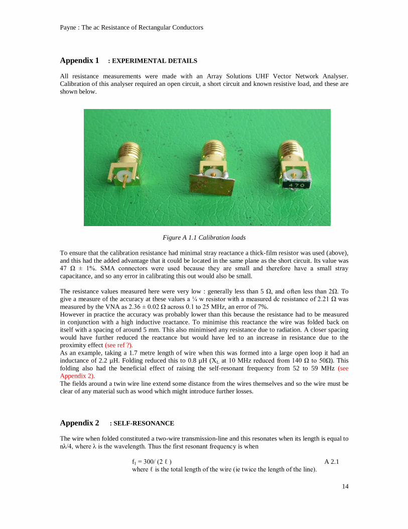
Payne : The ac Resistance of Rectangular Conductors
1
THE AC RESISTANCE OF RECTANGULAR CONDUCTORS
A simple equation is given here for the ac resistance of rectangular conductors. This is
shown to give good agreement with independent measurements for all shapes of
rectangular conductor from very thin strip to square section.
1. INTRODUCTION
A rigorous treatment of the ac resistance of conductors with a rectangular section leads to formidable
mathematical difficulties, and many authors have tried to overcome these problems over the past 100 years
but without success. Given that there is no useful theory the curves by Haefner (ref 1) are widely published,
and these are shown below. His paper was written in 1937 and so it is surprising that no analytical analysis
has replaced it.
The theoretical approach here is to simplify the problem by assuming that current diffuses from the four
faces independently. This along with experimentally derived factors give a simple equation which is shown
to be surprisingly accurate for all shapes of rectangular conductor from thin strip to square cross-section.
2. HAEFNER’S MEASUREMENTS
2.1. Published graphs
Haefner measured the ac resistance of five copper conductors having width to thickness (w/t) ratios of 1, 2,
5, 10, and 2400, and over a frequency range from 0 to 8 KHz. Each conductor was around 60 ft in length,
folded back on itself with a spacing of about 2ft which he had checked would have negligible proximity
effect. In addition to his own measurements he also used measurements published by other experimenters.
A summary of his findings is given in the graph below, extracted from Terman (ref 2) :
Figure 2.1 Haefner’s results
Payne : The ac Resistance of Rectangular Conductors
2
The other experimenters had used different sized conductors to his and measured them at different
frequencies, and so to combine all these measurements he used the principle of ‘similitude’. This had
previously been enunciated by Dwight who found that if measurements of resistance were plotted against
the parameter p = [8π f /(109 Rdc)]
0.5, the plot can be used to predict the resistance under different conditions
to the measurements. For instance measurements made on large conductors at low frequencies are valid for
small conductors at high frequencies and vice versa. The curve for the round wire above provides a good
example of the usefulness of this approach since only one curve is needed for round wire of any diameter,
and at any frequency.
Haefner also expresses p as
p = [8π f A/ ρa ]0.5
2.1.1
In this case the area is in cms2 and the specific resistance ρa is in absohms/cm
3, which for copper ρa =1724.
This is not in a convenient form today because the resistance R is expressed in absohms. It is easier and
more informative to re-write the parameter as :
p = A 0.5
/ (1.26 δ) 2.1.2
where A is the cross-sectional area in mm2
δ is the skin depth = [ρ/(πfµ)]0.5
in mm
It can now be seen that the parameter p is the ratio of two lengths, one related to the size of the conductor
and the other the skin depth. Notice that this equation includes the permeability, which in Haefner’s
equation is assumed to be unity.
The above curves are a combination of experimental and calculated results, with the dotted portions
representing the extrapolation of low frequency measurements to join some theoretical results by Cockroft
(ref 3) at high frequencies. These extrapolations could therefore be valid if Cockroft’s high frequency
theory was correct but this is unproven because he was unable to find any published measurements against
which to verify his theory. These extrapolations must be treated therefore with some caution.
The above graph is widely reproduced but not always with the dotted lines, so that it is then not clear that
much of the graph consists of extrapolations.
Note :
In some versions of the above graph the horizontal axis p is given as (f/Ro)0.5
, where f is in Hz and Ro is in
µΩ/m (for instance the Copper Association ref 4). Multiplying this factor by 1.58 gives p as defined by
Equation 2.1.1 or 2.1.2.
Alternatively p has been given in terms of (f/Ro 1000m)0.5
, where f is in Hz and Ro 1000m is the dc resistance of
1000 meter length. Dividing this equation by 20 gives p as defined by Equation 2.1.1 or 2.1.2.
2.2. Extrapolation of Haefner’s measurements
A large proportion of Haefner’s graph consists of extrapolations from measurements, and so it raises the
question as to how accurate these might be. Also further extrapolation may be necessary if his curves are to
used beyond the values given.
An insight into this extrapolation can be gained by considering the round conductor, because the resistance
of this is well understood and predictable. At very high frequencies the conducting area is a narrow band
around the circumference of the wire and of thickness equal to the skin depth δ. The conducting area is
therefore A= (π d δ). The ratio of the high frequency resistance to the low frequency resistance is thus equal
to the ratio of the conducting areas :
Rac/Rdc ≈ (πd2/4)/ (π d δ) = 0.25 d/δ 2.2.1
From Equation 2.1.2, p = d/ (1.48 δ). Thus the limiting value of the slope of Haefner’s round wire curve at
high frequencies should be by this calculation :
Limiting value of [(Rac/Rdc) / p] = 0.36 2.2.2
Payne : The ac Resistance of Rectangular Conductors
3
And indeed this is what it is. However we can anticipate that the curves for the rectangular conductors will
also have this same limiting slope. This will apply as long as the frequency is sufficiently high that ‘the
radius of curvature of the conductor surface is everywhere appreciably greater than the skin depth and does
not vary too rapidly around the periphery’ (Terman ref 2, page 34). Of course this can never be true for a
rectangular conductor with perfectly sharp corners, but a practical conductor will have rounded corners.
Indeed Haefner notes that the samples he measured had ‘… edges slightly rounded, as is the case in the
commercial production of such strip conductors’.
Indications of this limiting slope can be seen in Figure 2.1 where the slopes of the curves for w/t = 4 and
w/t = 8 are increasing towards that of the round conductor as p increases. The curve for w/t =16 also shows
this trend. The curve for w/t = 24 does not, but beyond p=5 it is linearly extrapolated and this may be
wrong. Indeed the theory presented here shows an increasing slope at this value of p (see comparisons
Section 6).
Cockroft’s analysis gives limiting slopes depending on the factor p. For instance for the square cross-
section he gives this as 0.418p for p>3.2, whereas Haefner’s curve is 0.37 p. For w/t = 8 Cockroft gives
0.29, whereas Haefner’s curve is 0.34 at p =10, and the slope is clearly still increasing (see ref 1 for
Cockroft’s data). So it would seem that Cockroft’s limiting values do not agree with experiment.
3. KEY FACTORS
3.1. Introduction
There are two key factors which determine the ac resistance of rectangular conductors : a) the diffusion of
current into the conductor from the four surfaces, and b) current crowding whereby the current concentrates
at the corners and edges. These are considered below.
3.2. Diffusion of current
It is well known that at high frequencies the current in a conductor tends to concentrate in a thin layer
around its surface. For instance a conductor with a circular cross-section carries current in only a thin layer
around its circumference, so that its high frequency resistance is the same as a hollow tube with a thickness
equal to the skin depth. At all points around this circumference this current has the same density.
Skin effect arises because current diffuses into a conductor from the outside. The amplitude of this current
is greatest at the surface and decreases exponentially with depth (ref 5):
Figure 3.2.1 Current density at depth
This exponentially decaying current has the same area as that of a current uniformly distributed down to
depth of δ, and zero at greater depths and this leads to the definition of skin depth :
Skin depth δ = [ρ/(πfµ)]0.5
3.2.1
Payne : The ac Resistance of Rectangular Conductors
4
There is some confusion in the literature over whether the skin effect is due to the penetration of
electromagnetic waves into the conductor or whether it is due to diffusion of current from the surface
(diffusion is defined as the movement from a high concentration to a lower concentration). This confusion
arises because the equation describing the attenuation through the conductor is the same (Equation 3.2.1).
While it is probable that EM waves do penetrate into a conductor the magnitude of the resultant current will
be many orders lower than that due to diffusion. Details are given in the author’s paper reference 6
Diffusion is a very very slow process, and for instance in copper at 1MHz it is about 415 metres per second,
or about a millionth of the velocity of EM waves in air (ref 7, p540). A current at 1 MHz has only 0.5 µs to
diffuse into the copper before the excitation reverses direction and in this time the current penetrates into
the copper by only 0.2 mm.
So this raises the question : if diffusion is so slow, how is energy transmitted along a conductor at a
velocity close to the speed of light? This has been answered recently by Edwards & Saha (ref 8) who show
that ‘ Currents are established on the surface of conductors by the propagation of electromagnetic waves in
the insulating material between them’ (my italics). This sets-up an excitation potential which travels along
the wire at the speed of light. ‘If it were not for the displacement current setting up the surface currents in
the first instance ……. energy transmission via copper conductors would be virtually impossible because of
the long diffusion process’.
Here it is assumed that diffusion into the four sides of the conductor are independent of one another and so
each can be treated in isolation.
3.3. Current Crowding
The resistance of a conductor is given by :
R = [ρ ℓ/A] 3.3.1
Where ρ is the resistivity of the conductor
ℓ is the length of the conductor
A is the conducting area
At very low frequencies the conducting area is equal to the cross-section of the conductor A = wt, where w
is the width and t is the thickness.
At very high frequencies, conduction takes place in a thin skin around the periphery of the conductor equal
in thickness to the skin depth δ , so the conducting area is then equal to Ac = 2 (w+t) δ. However this is not
the whole story for a rectangular conductor because in addition the current concentrates at the edges and the
corners. This effect is known as current crowding and is illustrated below :
Figure 3.3.1 Current crowding in a conductor with a rectangular section
Payne : The ac Resistance of Rectangular Conductors
5
1.0
1.5
2.0
2.5
3.0
3.5
1 10 100 1000
K
w/t
Current Crowding Factor K
Cockroft K
Haefner
Author's measurements
Figure 3.3.2 Current density in square section conductor
So the high frequency resistance is given by :
Rhf = KC [ ρ ℓ/(2 (w+t) δ] 3.3.2
where ρ is the resistivity of the conductor
ℓ is the length of the conductor
w is the conductor width
t is its thickness
δ is the skin depth
KC is the increase in resistance due to crowding
It is often convenient to express the ac resistance as the ratio to the dc resistance and Equation 3.3.2 then
becomes (ie dividing by Rdc = [ρ ℓ/(wt)]:
Rhf /Rdc = KC w t / [2 (w+t) δ] 3.3.3
The factor KC gives the increase in resistance due to current crowding. Terman (ref 2) gives a graph of KC,
calculated from Cockcroft (ref 3) ‘which will give reasonably accurate results when the thickness is
appreciably greater than twice the skin depth’ ie high frequencies.
This graph can be described by the following equation, plotted below.
KC = 1.06 + 0.22 Ln w/t + 0.28 (t/w)2 3.3.4
Figure 3.3.3 Current crowding factor KC
Payne : The ac Resistance of Rectangular Conductors
6
1.0
1.2
1.4
1.6
1.8
2.0
2.2
2.4
0.10 1.00 10.00 100.00
Kc
Haefner's factor P
Current Crowding Factor Kc
w / t =250
w / t =50
w / t =16
w / t =4
w / t =2
w / t =1
Current crowding occurs on all four faces of the conductor, and it is assumed that KC describes the
combined effect of all four.
Also plotted in red are points derived from Haefner’s curves. These are the values of KC required to make
Equation 3.3.3 equal to the values on the curve, when the thickness is appreciably greater than twice the
skin depth. Also plotted in green are the values of KC from the author’s measurements (see Section 6).
3.4. Variation of KC with Frequency
Neither Cockcroft nor Terman give the variation of KC with frequency, but clearly it has a value of unity at
very low frequencies. It is therefore useful to express it as KC = (1+x), where the factor x varies with
frequency and becomes zero at very low frequencies. So KC is conveniently expressed as :