Page 1
Certified in conformity Izmir, 22
nd June 2012
The General Director of the OIV Secretary of the General Assembly
Federico CASTELLUCCI
© OIV 2012 1
RESOLUTION OIV-VITI 423-2012 REV1
OIV GUIDELINES FOR VITIVINICULTURE ZONING METHODOLOGIES ON A SOIL AND
CLIMATE LEVEL
THE GENERAL ASSEMBLY,
On the proposal of Commission I “Viticulture”,
IN VIEW OF the works presented within the “Viticulture Environment and Climate
Change” expert group since 2007,
CONSIDERING
OIV Resolutions VITI/04/1998 and VITI/04/2006 that recommend that member countries
continue studying viticulture zoning,
CONSIDERING
Resolution OIV-VITI 333-2010 on the definition of vitivinicultural “terroir”,
CONSIDERING
The economic, legislative and cultural consequences related to vitiviniculture zoning,
CONSIDERING
That there is increasing interest in partaking in zoning operations in most viticulture
countries,
CONSIDERING
That there is a large spectrum of disciplines and tools used for carrying out zoning
studies which are not classified according to their objectives (or purpose or usage)
CONSIDERING
The necessity to establish a methodology that would allow member countries to choose
the most appropriate viticulture zoning method for their needs and goals,
CONSIDERING that “terroir” has a spatial dimension, which implies a need for
delimitation and zoning and that different aspects of terroir can be zoned, particularly
physical environment aspects: soil and climate,
CONSIDERING the importance, proposed by the CLIMA expert group and the Viticulture
Commission of having a single resolution on vitiviniculture zoning, divided into four parts,
(A, B, C, D)
DECIDES to adopt the following resolution, concerning the “OIV Guidelines for
vitiviniculture zoning methodologies on a soil and on a climate level”
Page 2
Certified in conformity Izmir, 22
nd June 2012
The General Director of the OIV Secretary of the General Assembly
Federico CASTELLUCCI
© OIV 2012 2
Foreword
The characteristics of a vitivinicultural product are largely the result of the influence of
soil and climate on the behaviour of the vine. Vitiviniculture zoning at soil and climate
level must be carried out consistently, for more relevance. Indeed, there are interactions
between climate and soil where the result may be decisive on the characteristics of a
product. For example, the water supply of vineyards is an illustration of this.
In the current proposal, the zoning steps appropriate to the soil and climate are
presented separately. This allows users to stagger the two types of zoning over time,
although for a good analysis of terroir both, as well as the interaction between them, are
essential.
PART A
OBJECTIVES OF VITIVINICULTURE ZONING ON A SOIL AND A CLIMATE LEVEL
Vitiviniculture zoning on a soil and a climate level can have different purposes. The prior
analysis of these purposes is a vital step in any zoning work. The methodology applied
must indeed be suited to the sought-after objectives (table 1).
Table 1: Objectives of vitiviniculture zoning and respective roles of the soil and climate
and their interaction (++: strong; +: intermediary; 0 none), for a given variety.
Zoning purpose Role
of the
soil
Role of
the
climate
Role of the
soil/climate
interaction
Delimitation of territories in accordance with their
potential to produce wine of a certain quality and
with certain typical features.
++ ++ ++
Zoning of the potential relative earliness (vine
development and grape ripening kinetic)
+ ++ 0
(cumulative
effect)
Optimisation of technical management by
adaptation of the plant material
++ ++ 0
Optimisation of technical and environmental
management by adaptation of growing practices
++ + +
Territorial management of crop protection risks + ++ +
Carry out land parcel selection ++ + 0
Territorial management of potential water
resources
++ ++ ++
Zoning of risks and strong climate constraints 0 ++ 0
Protection of terroirs and landscapes from various
threats and especially urbanisation
++ 0 0
Zoning in accordance with the aptitude of a
particular region for viticulture or for growing
particular varieties
+ ++ +
Page 3
Certified in conformity Izmir, 22
nd June 2012
The General Director of the OIV Secretary of the General Assembly
Federico CASTELLUCCI
© OIV 2012 3
PART B
OIV GUIDELINES FOR VITIVINICULTURE ZONING METHODOLOGIES ON A SOIL
LEVEL
A 3-step method
Step 1: Choose one or several approaches
Vitiviniculture zoning on a soil level may be based on one or more scientific disciplines:
geology, geomorphology or pedology.
- Geology enables a summary approach which is adapted to small scale zoning
(≤ 1/ 50,000e). Knowledge of local geology is critical prerequisite for soil
cartography. Geology doesn’t allow or allows very little to explain the functioning
of vines.
- Geomorphology enables a summary approach which is adapted to small scale
zoning (≤ 1/50,000e). Geomorphology facilitates the understanding of the
distribution of soil depth in a given region. Geomorphology doesn’t allow or allows
very little to explain the functioning of vines.
- Pedology (cartography of soil types) is an approach adapted to medium or large
scale zoning (≥ 1/25,000e). The creation of soil maps traditionally requires probes
with an auger and the study of soil profile pits. Pedology enables a link with the
functioning of the vine. It is recommended that the soil map is produced from the
“Soil Taxonomy” (American classification; USDA, 2010), the “World Reference
Base for Soil Resources” (FAO classification, 2006) or the Référentiel Pédologique
(French classification; Baize et Girard, 2009). If a local classification is used, a
match in one of the three classifications above shall be indicated. The interest and
limits of use of each of these three classifications are discussed in APPENDIX 1.
Certain disciplines can provide useful information for zoning but do not, as such, enable
viticulture soil zoning. Examples include botany (plants used as environment indicator).
Zoning can make use of several approaches simultaneously. The combination of a
geological, geomorphological and a pedological approach produces very applicable
zoning.
Page 4
Certified in conformity Izmir, 22
nd June 2012
The General Director of the OIV Secretary of the General Assembly
Federico CASTELLUCCI
© OIV 2012 4
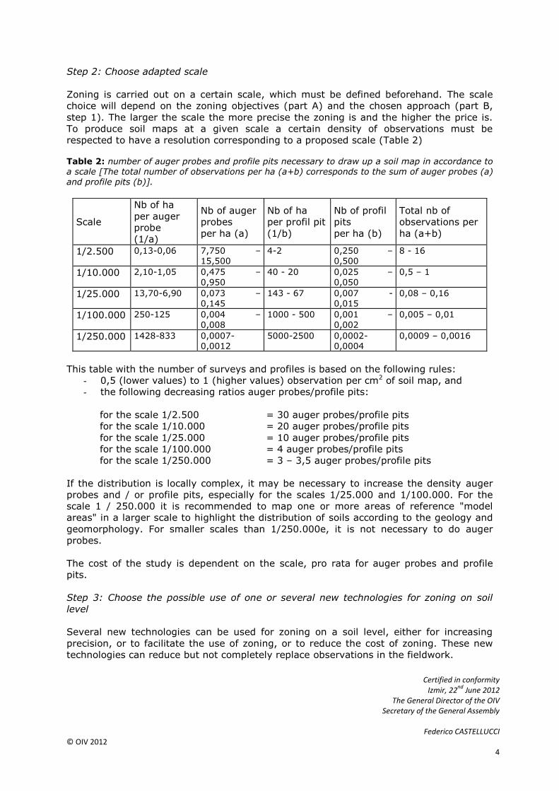
Step 2: Choose adapted scale
Zoning is carried out on a certain scale, which must be defined beforehand. The scale
choice will depend on the zoning objectives (part A) and the chosen approach (part B,
step 1). The larger the scale the more precise the zoning is and the higher the price is.
To produce soil maps at a given scale a certain density of observations must be
respected to have a resolution corresponding to a proposed scale (Table 2)
Table 2: number of auger probes and profile pits necessary to draw up a soil map in accordance to a scale [The total number of observations per ha (a+b) corresponds to the sum of auger probes (a) and profile pits (b)].
Scale
Nb of ha
per auger
probe
(1/a)
Nb of auger
probes
per ha (a)
Nb of ha
per profil pit
(1/b)
Nb of profil
pits
per ha (b)
Total nb of
observations per
ha (a+b)
1/2.500 0,13-0,06 7,750 –15,500
4-2 0,250 – 0,500
8 - 16
1/10.000 2,10-1,05 0,475 –
0,950 40 - 20 0,025 –
0,050 0,5 – 1
1/25.000 13,70-6,90 0,073 – 0,145
143 - 67 0,007 - 0,015
0,08 – 0,16
1/100.000 250-125 0,004 –
0,008 1000 - 500 0,001 –
0,002 0,005 – 0,01
1/250.000 1428-833 0,0007-0,0012
5000-2500 0,0002-0,0004
0,0009 – 0,0016
This table with the number of surveys and profiles is based on the following rules:
- 0,5 (lower values) to 1 (higher values) observation per cm2 of soil map, and
- the following decreasing ratios auger probes/profile pits:
for the scale 1/2.500 = 30 auger probes/profile pits
for the scale 1/10.000 = 20 auger probes/profile pits
for the scale 1/25.000 = 10 auger probes/profile pits
for the scale 1/100.000 = 4 auger probes/profile pits
for the scale 1/250.000 = 3 – 3,5 auger probes/profile pits
If the distribution is locally complex, it may be necessary to increase the density auger
probes and / or profile pits, especially for the scales 1/25.000 and 1/100.000. For the
scale 1 / 250.000 it is recommended to map one or more areas of reference "model
areas" in a larger scale to highlight the distribution of soils according to the geology and
geomorphology. For smaller scales than 1/250.000e, it is not necessary to do auger
probes.
The cost of the study is dependent on the scale, pro rata for auger probes and profile
pits.
Step 3: Choose the possible use of one or several new technologies for zoning on soil
level
Several new technologies can be used for zoning on a soil level, either for increasing
precision, or to facilitate the use of zoning, or to reduce the cost of zoning. These new
technologies can reduce but not completely replace observations in the fieldwork.
Page 5
Certified in conformity Izmir, 22
nd June 2012
The General Director of the OIV Secretary of the General Assembly
Federico CASTELLUCCI
© OIV 2012 5
- Geographic Information Systems (G.I.S.) provide a computerised read out of
zoning results which enables the layering of several levels of information with the
possibility of inserting non spatial information.
- Numerical Terrain Models (N.T.M.) able to carry out precise geomorphological
studies at a moderate cost.
- The geophysical approach (measurement of electrical conductivity of the soil)
enables increased soil map precision by limiting the number of probes or profile
pits necessary for carrying out the approach. This technology is particularly
adapted to carrying out large scale zoning works. (≥1/5,000e)
- Remote sensing enables the interpretation of soil surface on non planted land
parcels with no vegetation.
- The geostatistical approach enables the transformation of point to point basis
information into spatial information.
Page 6
Certified in conformity Izmir, 22
nd June 2012
The General Director of the OIV Secretary of the General Assembly
Federico CASTELLUCCI
© OIV 2012 6
PART C
OIV GUIDELINES FOR VITIVINICULTURE ZONING METHODOLOGIES ON A
CLIMATE LEVEL
A 3-step method
Stage 1: Select appropriate climatic indicators for the purpose
Vitiviniculture zoning on a climate level is done on the basis of various indices derived
from analysis of climate data. The choice of which data, which data source and which
indices to use depends on which are most suitable for the purposes mentioned in part A
(see table 3) as well as their availability.
Table 3: Climate data and bioclimatic indices to be used depending on the purpose of
the climate-based vitiviniculture zoning:
Purpose of zoning or
analysis criteria
Climate data and biolimatic indices
adapted to the zoning’s purpose
Timescale
required
Relative earliness GDD, AvGST Month, day, hour
Potential of a territory in
producing wines of a
certain type
WB, RR (flowering-harvest), ET0, AMP.,
Min,GDD, AvGST Month, day, hour
Water management WB, RR (vegetative period), ET0 Month, day, hour
Crop protection threats TM, RH, DH, Phytosanitary risks models Day, hour
Frost threat TN, TS, GDD Day, hour
Hail threats Hail pads, meteorological radar Day, hour
Extreme heat threat TX Day, hour
Wind problems W Day, hour
ACRONYMS USED:
AvGST: Average growing season temperature; WB: water balance (moisture balance);
DH: Duration of humidification; ET0: Reference (potential) evapotranspiration; GDD:
Growing degree days and its derivatives (Winkler’s index, Huglin’s index,...); AMP:
Indices based on the temperature range in the ripening period; MIN: Indices based on
temperature minimums in the ripening period; RH: Relative humidity; RR: Cumulative
rainfall; TM : Average air temperature; TN: Minimum temperature; TS: Surface
temperature; TX: Maximum temperature, W: wind speed.
For the purpose of comparison with other zoning operations performed at other sites or
at other times, it is useful to work wherever feasible with commonly used, relevant
indicators (see APPENDIX 2).
Stage 2: Select high quality climate data sources that are suitable for climatic zoning.
There are three possible sources of climate data: data recorded by weather stations,
remote sensing data (satellite and radar) and data produced by dynamic models (general
circulation models [GCMs] or regional dynamic models).
Page 7
Certified in conformity Izmir, 22
nd June 2012
The General Director of the OIV Secretary of the General Assembly
Federico CASTELLUCCI
© OIV 2012 7
Most of the relevant indicators needed for zoning according to climate can be obtained
from the data recorded by weather stations. It will be necessary in the first instance:
- to assess the quality of the recording sites, in order to ascertain the uniformity of
the climate signal recorded (avoid any microclimate influence at the weather
station);
- to identify and eliminate any atypical or false data.
These climate data or the derived relevant indices are punctual. Spatialisation of these
data is essential prior to zoning. It consists of estimating the value of a bioclimatic
variable or index for each point within the area in question based on measuring points.
There are two possible ways of doing this: subjective demarcation, based on the
cartographer’s expertise and spatial interpolation of the climate data.
It is essential to work out the uncertainty associated with the interpolation, using a data
set for validation that is separate from the one used for the data interpolation or by
performing a ‘leave-one-out’ type cross-validation.
Remote sensing provides climate data over large spatial scales and over a continuous
timescale. These data often need to be pre-processed before they are used in the context
of vitiviniculture zoning (elimination of artefacts such as cloud cover, calculation of
indices using data measured on the soil, etc.). It is also important to check the quality of
the data, especially with regard to the spatial and temporal uniformity of the signal being
analysed (for example for zoning based on different satellite images).
Dynamic models (or models of regional / global circulation) produce very large quantities
of climate data, covering a wide spatial scale (whole world). However, the spatial
resolution of the data is relatively low (between 50 and several hundred kilometres) and
assessing the quality of the data produced by these models is problematic from the
methodological point of view (pixel size / weather station comparison).
Stage 3: Identify climatically homogeneous zones
Unlike vitiviniculture zoning on the soil level, which relies in most instances on qualitative
soil type data, zoning according to climate is based on ongoing quantitative data.
Homogeneous zones therefore need to be demarcated according to some climate
parameters. Spatial variability in the climatically homogeneous zones must be greater
than or equal to the mapping error. It is also desirable that the areas should be
demarcated according to criteria that are relevant for viticulture and are able to be
substantiated during a subsequent verification stage. In other words, establishing climate
data categories whose variations are irrelevant for viticulture should be avoided.
Furthermore, since climate can vary considerably over time, vitiviniculture zoning
according to climate must be based on descriptive statistics calculated over a sufficient
number of years for the zoning to be credible. The number of years required depends on
the purpose of the zoning, the variable in question and the factors responsible for its
variations in space (see APPENDIX 3).
Finally a qualitative method for climatic zoning may be considered, using analysis of the
landscape (enclosure index of the countryside, radiation balance). This method may be
implemented with the help of a digital analysis of the relief (digital terrain models) and
Geographical Information Systems. It is a more subjective approach but dispenses with
Page 8
Certified in conformity Izmir, 22
nd June 2012
The General Director of the OIV Secretary of the General Assembly
Federico CASTELLUCCI
© OIV 2012 8
the need for climate data, hence it is easier to implement. On the other hand, it is
inherently limited due to the absence of quantitative measurements of the variables
under study.
Page 9
Certified in conformity Izmir, 22
nd June 2012
The General Director of the OIV Secretary of the General Assembly
Federico CASTELLUCCI
© OIV 2012 9
PART D
VALIDATION METHODS OF VITIVINICULTURE ZONING ON A SOIL AND ON A
CLIMATE LEVEL
Depending on the sought-after objectives, the relevance of vitiviniculture zoning on a soil
and on a climate level can be validated by various methods:
- By eco-physiology studies. These methods focus on the response of vines to
environmental factors. They allow an explanation of vine functioning in relation to
the soil on the level of the water regime of the territory in question and that of the
vine, its mineral alimentation (especially nitrogen), its phenology, its vegetative
expression and the grapes maturation. They can be either punctual (a network of
reference plots) or spatialised (maps of vigour, of precocity, of water regime, of
nitrogen alimentation, of components of grapes in maturity...).
- By land parcel surveys to study the relationship between the empirical knowledge
of producers and the viticulture potential.
- By sensory analysis of the quality and the typical features of the grape and the
wine obtained, either by large scale winemaking or by micro-vinification.
- For zoning related to climate or pest risks, by comparing the damage observed on
the plots to the risk level delivered by the maps.
This validation step can be assisted by new technologies. Vigour and growing kinetics can
be obtained by remote sensing or close-up detection using built-in sensors on agricultural
machines that are localised by G.P.S. Geo statistics enable the transformation of point to
point basis information into spatialised information, under the condition that the density
of the point to point basis information is sufficiently high. The Geographic Information
Systems (G.I.S.) allow to cross the levels that come from the zoning with the levels of
information obtained by the validation step.
The reproduction of the results from zoning on a soil and/or a climate level must satisfy
the sought-after objectives, i.e. be carried out on a scale adapted to and format usable
by the end users. The reproduction formats can therefore vary from global reports for
administrative decision-makers to land parcel management software for large-scale
studies that can be used directly by wine growers.
CONCLUSIONS
Numerous approaches exist for zoning on a soil level while making use of various
scientific disciplines at various scales with the support of more or less new technologies.
The approach and the scale to choose depend on the objectives that have to be defined
in advance.
A scale of 1/5,000e is suitable for zoning on a soil level of around ten to one hundred
hectares while a scale ranging from 1/10,000e to 1/25,000e is suitable for zoning an
appellation. Above the scale 1/25,000e, soil zoning loses its interest because it becomes
inevitable that several types of soil per unit of legend have to be combined.
The most relevant zonings at soil level are the ones resulting from a multi-discipline
approach: geology, geomorphology and pedology;
Page 10
Certified in conformity Izmir, 22
nd June 2012
The General Director of the OIV Secretary of the General Assembly
Federico CASTELLUCCI
© OIV 2012 10
The quality of the source data is a vital factor for climatic zoning. Uncertainties
associated with measurements, particularly those on a large scale, can sometimes be
greater than the spatial variability of the indicator being studied. In addition, the
mapping procedure (spatial scaling of data) can lead to significant calculation errors on
top of the uncertainties linked with the metering equipment or the microclimate
conditions at the weather station. It is therefore essential to evaluate the overall
uncertainty associated with the method alongside the climatic zoning procedure.
Zoning can be validated using phenological observation, ecophysiological measurement,
analysis of the wine, economic information, or new technologies such as remote sensing.
Surveys among wine growers may potentially help the results of the validation.
Vitiviniculture zoning remains a tool, where the interest and relevance is partly measured
by its ease of use and its ability to satisfy the expectations of the recipients.
Page 11
Certified in conformity Izmir, 22
nd June 2012
The General Director of the OIV Secretary of the General Assembly
Federico CASTELLUCCI
© OIV 2012 11
APPENDIX 1: Interest of the various soil classifications recommended for
vitiviniculture zoning on a soil level
There are many soil classifications. For standardisation, the OIV recommends that its
members use one of the following three classifications for vitiviniculture zoning works:
the “Soil Taxonomy” (American classification; USDA, 2010), the “World Reference Base
for Soil Resources” (FAO Classification, 2006) or the Référentiel Pédologique (French
classification; Baize et Girard, 2009). Each of these classifications has interests and limits
of use.
The “Soil Taxonomy” (American classification; USDA, 1993, 1999, 2010) is the
classification which allows the most accurate definition of the soil types encountered. It is
used in many countries. However, its complexity makes it a tool for specialist soil experts
rather than for use by anyone likely to carry out vitiviniculture zoning works.
The “World Reference Base for Soil Resources” (FAO classification, 2006), also called the
FAO classification, is an internationally recognised classification which is simple to use.
However, the number of references proposed is limited (only 32). Furthermore, this
classification does not recognise the predominant role of the rock type in the
pedogenesis. Consequently, there is no group of carbonated soils, which is limiting for
zoning in vitiviniculture.
The Référentiel Pédologique (French classification; Baize et Girard, 2009) is a relatively
comprehensive and easy to use reference. It is based on both morphological criteria
(diagnosis horizon) and pedogenetic elements (type of parent rock in particular). Even
though this classification is used in several countries, its national origin (French) is a
limit.
Page 12
Certified in conformity Izmir, 22
nd June 2012
The General Director of the OIV Secretary of the General Assembly
Federico CASTELLUCCI
© OIV 2012 12
APPENDIX 2: Bioclimatic indices currently used in the practice of vitiviniculture
zoning
There are a very large number of indices that can be used for climatic vitiviniculture
zoning, where the calculation relies on eco-physical concepts and the more or less
sophisticated resulting models. Among the most complex, mechanistic cultivation models
allow the most realistic assessment of the influence on the climate on vine development
and grape ripening (Bindi and Maselli, 2001; Carcia de Cortazar Atauri, 2006). Their main
inconvenience is the high degree of technical ability that they require, involving expert
knowledge in the user. Conversely, the very simple indicators, such as average growing
season temperature (Jones et al., 2004), are more or less relevant from a biological point
of view but are accessible to a wide audience. There is no denying that in the scientific
and technical literature, the most commonly used indices within the framework of
characterisations or climatic zoning of vitivinicultural environments use relatively simple
models on semi-empirical or mechanistic bases (Amerine and Winkler, 1944; Dumas et
al., 1997; Jacquet and Morlat, 1997; Tonietto and Carbonneau, 1998; Bois et al., 2008).
The most often used concepts are: extreme temperatures (freezing temperatures of the
vegetative parts, wood and buds, extreme heat), cumulative temperatures, the water
balance and minimum temperatures and/or temperature variations in the grape ripening
period. Depending on the objectives of zoning, it may be appropriate to focus on a multi-
criteria approach by combining indices providing complementary information (such as,
for example, the Multicriteria Climatic Classification proposed by Tonietto, 1999 and
Tonietto and Carbonneau, 2004).
Risk indicators based on extreme temperatures
- Minimum freezing temperature during the vine’s dormant period.
This is the minimum temperature below which irreversible damage to the viability of the
buds or the entire vine can be observed. Depending on the plant material and the
hardness of the vine, the vine’s resistance threshold at low temperatures ranges from -
15°C and -25°C (Düring, 1997; Lisek, 2009).
- Minimum freezing temperature during the growing period.
The destruction of the vegetative organs by frost depends on the developmental stage of
the vine and plant material (Fuller and Telli, 1999). The damage usually appears below -
3°C. In temperate climates, these situations sometimes occur in conditions such as
"radiation frost" associated with a reversal of the standard altitudinal gradient: the
temperature under shelter (1.5 or 2m) sometimes markedly very different from the
conditions observed in the vegetative organs (Guyot, 1997). For these reasons, we
consider 0°C to -2°C under cover as a freezing temperature in the growing season.
- Maximum temperature during the growing and grape ripening period
The consequences of high temperatures on the vine vary depending on their duration,
water resources, the vegetative stage and the genotype of the graft (Matsui et al., 1986,
Sepulveda et al., 1986a, 1986b). In addition, they do not necessarily have a negative
impact on the physiology of the vine and the ripening of the grapes (Hüglin and
Schneider, 1998). We can nevertheless consider that beyond 35°C, the photosynthetic
capacity of the vine decreases and the anthocyanin content of grapes is affected (Spayd
et al. 2002; Kliewer, 1977).
Indices based on the growing season air temperature, indicators of vine
development and grape ripening kinetic.
Page 13
Certified in conformity Izmir, 22
nd June 2012
The General Director of the OIV Secretary of the General Assembly
Federico CASTELLUCCI
© OIV 2012 13
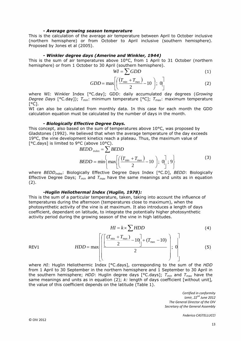
- Average growing season temperature
This is the calculation of the average air temperature between April to October inclusive
(northern hemisphere) or from October to April inclusive (southern hemisphere).
Proposed by Jones et al (2005).
- Winkler degree days (Amerine and Winkler, 1944)
This is the sum of air temperatures above 10°C, from 1 April to 31 October (northern
hemisphere) or from 1 October to 30 April (southern hemisphere).
GDDWI (1)
0;10
2max maxmin TT
GDD (2)
where WI: Winkler Index [°C.day]; GDD: daily accumulated day degrees (Growing
Degree Days [°C.day]); Tmin: minimum temperature [°C]; Tmax: maximum temperature
[°C].
WI can also be calculated from monthly data. In this case for each month the GDD
calculation equation must be calculated by the number of days in the month.
- Biologically Effective Degree Days.
This concept, also based on the sum of temperatures above 10°C, was proposed by
Gladstones (1992). He believed that when the average temperature of the day exceeds
19°C, the vine development kinetics reach a plateau. Thus, the maximum value of
[°C.days] is limited to 9°C (above 10°C).
9;0;102
maxmin maxmin TTBEDD
BEDDBEDD index
(3)
where BEDDindes: Biologically Effective Degree Days Index [°C.D], BEDD: Biologically
Effective Degree Days; Tmin and Tmax have the same meanings and units as in equation
(2).
-Huglin Heliothermal Index (Huglin, 1978):
This is the sum of a particular temperature, taken, taking into account the influence of
temperatures during the afternoon (temperatures close to maximum), when the
photosynthetic activity of the vine is at maximum. It also introduces a length of days
coefficient, dependant on latitude, to integrate the potentially higher photosynthetic
activity period during the growing season of the vine in high latitudes.
HDDkHI (4)
REV1
0;2
)10(102
)(
max
maxmaxmin T
TT
HDD (5)
where HI: Huglin Heliothermic Index [°C.days], corresponding to the sum of the HDD
from 1 April to 30 September in the northern hemisphere and 1 September to 30 April in
the southern hemisphere; HDD: Huglin degree days [°C.days]; Tmin and Tmax have the
same meanings and units as in equation (2); k: length of days coefficient [without unit],
the value of this coefficient depends on the latitude (Table 1).
Page 14
Certified in conformity Izmir, 22
nd June 2012
The General Director of the OIV Secretary of the General Assembly
Federico CASTELLUCCI
© OIV 2012 14
Table 1: value of the length of days coefficient k for several latitude ranges
Latitude 40 to 42° 42.1 to 44° 44.1 to
46°
46.1 to
48°
48.1 to 50°
Value of k 1.02 1.03 1.04 1.05 1.06
NB: the value of k is not proposed above and below the latitudes 40 and 50°. Current
works are expected to lead to new proposed values for k coefficients for lower and higher
latitudes than those originally involved in the calculation of HI.
Indices based on night temperatures and/or the temperature range, indicators
of grape ripening conditions
- Cool Night Index (CNI)
The Cool Night Index was proposed by Tonietto (1999) and Tonietto and Carbonneau
(2004). It corresponds to the average minimum temperature (°C) in September in the
northern hemisphere and March in the southern hemisphere.
The minimum temperatures during the period of ripening of the grapes of each variety /
region can also be included, so as to consider the local conditions.
- Fregoni Index (simplified)
On the same principle, Fregoni (Fregoni and Pezzutto, 2000) proposed an index
incorporating both the diurnal temperature range and the length of the period during
which the temperature stays below 10°C, for a period of 30 days prior to grape maturity.
Proposed on the basis of hourly temperatures, the simplified version is applicable to daily
climate data:
10minmax dTNTTIFs (4)
where IFs: Simplified Fregoni index [°C.days]; Tmin and Tmax have the same meanings
and units as in equation (2); Nd<10: number of days where the average temperature is
below 10°C.
Vitiviniculture climatic water balance, indicator of the water offer at climate
level:
- Drought index:
This is an adaptation by Tonietto (1999) of the Water balance by Riou (1994). The water
balance is calculated in monthly stages, over a period of six months between 1 April and
30 September (northern hemisphere) or between 1 October and 31 March (southern
hemisphere). Its value at the "cycle" end (30 September for the northern hemisphere
and 31 March for the southern hemisphere) is the drought index:
6 mWIS (5)
where IS: drought index [mm]; Wm=6: value of the water balance [in mm] at the end of
the sixth month m.
The water balance for each of the six months is calculated as follows:
01 ;min WETPWW svmm (5)
Page 15
Certified in conformity Izmir, 22
nd June 2012
The General Director of the OIV Secretary of the General Assembly
Federico CASTELLUCCI
© OIV 2012 15
where Wm: water balance at the end of month m; Wm-1: water balance at the end of the
previous month; P: total monthly precipitation for the month m;Tv: transpiration of the
vine for month m; Es: evaporation at soil level during month m; W0: useful reserve in the
soil set to 200 mm. All these sizes are expressed in mm.
When m=1, i.e. the first month of the water balance calculation, the amount of water
available in the soil the previous month (Wm-1 or W0) is considered to be equal to the
useful reserve W0 which is 200 mm.
NB: Wm may have a negative value. This conceptual approach is proposed for a better
characterization of the importance of a possible deficit in water resources for the vine.
Vine transpiration is assessed each month based on the development stage of the vine
and the evaporative demand of the atmosphere:
0ETkTv (6)
where ET0: cumulative reference evapotranspiration for the month m (or potential
evapotranspiration, [mm]); k: interception coefficient for the solar radiation by the vine’s
plant covering, changing monthly depending on the vine’s growth stage (table 2).
Table 2: value of the coefficient k for the 6 months of calculating the drought index
Month number 1 2 3 to 6
Northern
hemisphere
April May June to
September
Southern
hemisphere
October November December to
March
K Value 0.1 0.3 0.5
Soil evaporation is the fraction of ET0 not consumed by the vine, or (1-k) x ET0) for the
period during which the surface part of the soil is still wet. The duration of this period is
assessed based on monthly precipitation P. It corresponds to a fifth of the cumulative
rain for the month m in days:
md
md
s NP
kN
ETE ,
,
0 ;5
max1 (7)
where Nd,m: number of days in the month m.
Page 16
Certified in conformity Izmir, 22
nd June 2012
The General Director of the OIV Secretary of the General Assembly
Federico CASTELLUCCI
© OIV 2012 16
APPENDIX 3: Note on the temporal sample necessary for the use of bioclimatic
indices with the objective of vitiviniculture zoning on a climate level
The climate differs from the soil in particular due to its temporal variability. Also its
characterization, for vitiviniculture zoning in terms of the bioclimatic indices used,
requires a study over several years. The size of this temporal sample, hereafter referred
to as the “study duration”, is highly dependent on the objectives defined. There are 2
cases, among others:
- The zoning objective is limited solely to the identification of areas considered
as climatically homogeneous (in terms of one or more agroclimatic indices) within
the study area.
- The zoning objectives are (1) to distinguish areas considered climatically
homogeneous within the study area, (2) to compare the climatic characteristics of
areas identified in the study area with other wine regions (intra- and extra-
regional comparison)
In the first case, the study duration can be variable, depending on the spatial scale and
the atmospheric and environmental factors that govern the spatial variability of the
climate. Thus, for large-scale zoning (study area of a size less than 100 km), certain
variables such as air temperature may be affected, in some areas, primarily by lasting
geographical elements or those that are only slightly variable over time, such as the
relief or land use. Thus, a study period of several years (5 years minimum) may be
sufficient to demonstrate redundant spatial structures over the years. However, for
variables where the spatial distribution depends largely on weather conditions, such as
rainfall, a substantial study duration is required. It is recommended that the times given
for the calculation of climate normals, as defined by the World Meteorological
Organization (WMO, 1989; Argue and Vose, 2011) are used, which is 30 years.
In the second case, it is also recommended that a study period of 30 years is used. It is
clear that the comparison of the climatic characteristics of the areas identified in the
study area with other wine regions requires identical periods of study, due to climate
change over the long term.
Page 17
Certified in conformity Izmir, 22
nd June 2012
The General Director of the OIV Secretary of the General Assembly
Federico CASTELLUCCI
© OIV 2012 17
Bibliographical references:
Amerine, M.A., et A.J. Winkler. 1944. Composition and quality of musts and wines of
California grapes. Hilgardia. 15(6): 493-673.
Arguez, A., et Vose, R.S., 2011. The Definition of the Standard WMO Climate Normal:
The Key to Deriving Alternative Climate Normals. Bulletin of the American
Meteorological Society 92: 699-704.
Baize D. et Girard M.-C. 2009. Référentiel Pédologique 2008. Ed. Quae, France, 406p.
Bindi, M., et F. Maselli. 2001. Extension of crop model outputs over the land surface by
the application of statistical and neural network techniques to topographical and
satellite data. Climate Research. 16: 237-246.
Bois, B., C. Van Leeuwen, P. Pieri, J.P. Gaudillère, E. Saur, D. Joly, L. Wald, et D. Grimal.
2008. Viticultural agroclimatic cartography and zoning at mesoscale level using
terrain information, remotely sensed data and weather station measurements.
Case study of Bordeaux winegrowing area. Dans VIIème Congrès International
des Terroirs viticoles. Nyons (Switerzland).
Dumas, V., E. Lebon, et R. Morlat. 1997. Différenciations mésoclimatiques au sein du
vignoble alsacien. Journal International des Sciences de la Vigne et du Vin. 31(1):
1-9.
Düring, H. 1997. Potential frost resistance of grape: Kinetics of temperature-induced
hardening of Riesling and Silvaner buds. Vitis. 36(4): 213-214.
Fregoni, M., Pezzutto S. 2000. Principes et premières approches de l'indice de qualité
Fregoni. Progr.Agric.Vitic. 117: 390-396.
Fuller, M.P., et G. Telli. 1999. An investigation of the frost hardiness of grapevine (Wis
vinvera) during bud break. Annals of Applied Biology. 135: 589-595.
Garcia de Cortazar Atauri, I. 2006. Adaptation du modèle STICS a la vigne (Vitis vinifera
L.). Utilisation dans le cadre d'une étude d'impact du changement climatique a
l'échelle de la France. Thèse de doctorat, Ecole Nationale Supérieure Agronomique
de Montpellier, Montpellier (France), 292p.
Guyot, G. 1997. Climatologie de l'environnement. De la plante aux ecosystèmes. Éd.
Masson, Paris, 544p.
Huglin, P. 1978. Nouveau mode d'évaluation des possibilités héliothermiques d'un milieu
viticole. Comptes Rendus de l'Académie de l'Agriculture de France. 64: 1117-
1126.
Huglin, P., et C. Schneider. 1998. Biologie et écologie de la vigne. Éd. Lavoisier, Paris,
370p.
Jacquet, A., et R. Morlat. 1997. Caracterisation de la variabilité climatique des terroirs
viticoles en val de Loire. Influence du paysage et des facteurs physiques du
milieu. Agronomie. 17(9/10): 465-480.
Jones, G.V., P. Nelson, et N. Snead. 2004. Modeling Viticultural Landscapes: A GIS
Page 18
Certified in conformity Izmir, 22
nd June 2012
The General Director of the OIV Secretary of the General Assembly
Federico CASTELLUCCI
© OIV 2012 18
Analysis of the Terroir Potential in the Umpqua Valley of Oregon. Geoscience
Canada. 31(4): 167-178.
Jones, G.V., M.A. White, O.R. Cooper, et K. Storchmann. 2005. Climate change and
global wine quality. Climatic Change. 73(3): 319-343.
Kliewer, W.M. 1977. Influence of temperature, solar radiation and nitrogen on coloration
and composition of Emperor grapes. American Journal of Enology and Viticulture.
28(2): 96-103.
Lisek, J. 2009. Frost damage of buds on one-year-old shoots of wine and table grapevine
cultivars in Central Poland following the winter of 2008/2009. Journal of Fruit and
Ornamental Plant Research. 17(2): 149-161.
Matsui, S., K. Ryugo, et W.M. Kliewer. 1986. Growth inhibition of Thompson Seedless
and Napa Gamay berries by heat stress and its partial reversibility by applications
of growth regulators. American Journal of Enology and Viticulture. 37(1): 67-71.
Riou, C. 1994. Le déterminisme climatique de la maturation du raisin: application au
zonage de la teneur en sucre dans la Communauté Européenne (E Commission,
Éd.). Publications Office of the European Union, Luxembourg, 322p.
Sepulveda, G., et W.M. Kliewer. 1986. Effect of high temperature on grapevines (Vitis
vinifera L.). II. Distribution of soluble sugars. American Journal of Enology and
Viticulture. 37(1): 20-25.
Sepulveda, G., W.M. Kliewer, et K. Ryugo. 1986. Effect of high temperature on
grapevines (Vitis vinifera L.). I. Translocation of 14C-photosynthates. American
Journal of Enology and Viticulture. 37(1): 13-19.
Spayd S., Tarara J., Mee D. and Ferguson J., 2002. Separation of sunlight and
temperature effects on the composition of Vitis vinifera cv. Merlot berries. Am. J.
Enol. Vitic., 53, 171-182.
Tonietto, J. 1999. Les Macroclimats Viticoles Mondiaux et l'Influence du Mésoclimat sur la
Typicite de la Syrah et du Muscat de Hambourg dans le Sud de la France -
Méthodologie de Caractérisation. Thèse de doctorat, Ecole Nationale Supérieure
Agronomique de Montpellier, Montpellier (France), 216p.
Tonietto, J., et A. Carbonneau. 1998. Facteurs mésoclimatiques de la typicité du raisin de
table de l'A.O.C. Muscat du Ventoux dans le département du Vaucluse, France.
Progres Agricole et Viticole. 115(12): 271-279.
Tonietto, J., et A. Carbonneau. 2004. A multicriteria climatic classification system for
grape-growing regions worldwide. Agricultural and Forest Meteorology. 124(1/2):
81-97.
WMO, 1989. Calculation of Monthly and Annual 30-Year Standard Normals ( No. WCDP-
No. 10, WMO-TD/No. 341). World Meteorological Organization
World Reference Base for Soil Resources, 2006. A framework for International
Classification, Correlation and Communication, Food and Agricultural Organisation
of the United Nations, 128 p.
Page 19
Certified in conformity Izmir, 22
nd June 2012
The General Director of the OIV Secretary of the General Assembly
Federico CASTELLUCCI
© OIV 2012 19
United States Department of Agriculture, Natural Resources Conservation Services, 1993.
Soil Survey Manual. Division Staff, 318 p.
United States Department of Agriculture, Natural Resources Conservation Services, 1999.
Soil taxonomy. A basic system of soil classification for making and interpretation
of soil surveys. Superintendent of Documents, U.S. Government Printing Office,
Washington, DC 20402, 870 p.
United States Department of Agriculture, Natural Resources Conservation Services, 2010.
Keys to Soil Taxonomy. Soil Survey Staff. Eleventh Edition.